modular cam program development for single …
TRANSCRIPT
The Pennsylvania State University
The Graduate School
MODULAR CAM PROGRAM DEVELOPMENT FOR SINGLE POINT DIAMOND
TURNING OF FREEFORM OPTICS
A Thesis in
Mechanical Engineering
by
Zachary N. Timothy
2021 Zachary N. Timothy
Submitted in Partial Fulfillment of the Requirements
for the Degree of
Master of Science
May 2021

The thesis of Zachary N. Timothy was reviewed and approved by the following:
Eric Marsh Glenn Professor of Engineering Education Thesis Advisor
Guha Manogharan Emmert H. Bashore Faculty Development Assistant Professor
Karen A. Thole Distinguished Professor and Head of Mechanical Engineering

iii
ABSTRACT
As optic designs have increased in sophistication over the past decades, freeform optics
have proven highly valuable for being able to increase design performance while decreasing
weight and components needed. Through the development of this technology, many approaches
have been developed for the most accurate toolpath generation in different applications. In this
thesis, single point diamond turning is reviewed, and a modular CAM program was developed in
MATLAB that has the framework to expand and incorporate these many approaches. All the
CAM functionalities for single point diamond turning included in this program are examined in
further depth in the subsequent sections including toolpath generation, calculation of cutter
locations, post processing, and helpful program checks. The program was then verified by turning
a diverse set of four freeform optics on a Moore Nanotechnology UPL 350.

iv
TABLE OF CONTENTS
LIST OF FIGURES ..................................................................................................................... vii
LIST OF TABLES ......................................................................................................................... x
ACKNOWLEDGEMENTS ........................................................................................................ xii
Chapter 1 Introduction ................................................................................................................. 1
1.1 Freeform Surfaces .............................................................................................................. 1 1.2 Freeform Surface Applications .......................................................................................... 3 1.3 Diamond Machining Methods ........................................................................................... 5
1.3.1 Fast Tool Servo ...................................................................................................... 5 1.3.2 Slow Slide Servo .................................................................................................... 7
Capabilities of the Moore Nanotechnology UPL 350 ............................................. 8 1.4 Diamond Turning Workflow ............................................................................................. 8 1.5 CAM Program Considerations ........................................................................................... 9
Chapter 2 CAM Program Framework and Features .............................................................. 11
2.1 CAM Essential Functions and Workflow ........................................................................ 11 2.2 Core Modular Framework ............................................................................................... 12
Chapter 3 Toolpath Generation................................................................................................. 16
3.1 Working in Cylindrical Coordinates ................................................................................ 16 3.2 Generating the Base Spiral .............................................................................................. 17
3.2.1 Archimedean Spirals ............................................................................................. 17 fcn_ArchimedesSpiral ........................................................................................... 19
3.2.2 Space Archimedean Spiral .................................................................................... 20 3.3 Surface Descriptions ........................................................................................................ 21
3.3.1 Aspheric Surface ................................................................................................... 22 3.3.2 NURBS Surfaces .................................................................................................. 22 3.3.3 Zernike Polynomials ............................................................................................. 22
fcn_Zernike ........................................................................................................... 24 3.4 Mapping Spiral to Surface ............................................................................................... 25 3.5 Cutter Radius Compensation ........................................................................................... 26
3.5.1 Oscillating X Cutter Compensation ...................................................................... 26 fcn_OscXCutterComp ........................................................................................... 27
3.5.2 Steady X Cutter Compensation ............................................................................ 28 fcn_SteadyXCutterComp ...................................................................................... 29
3.5.3 Golden Point Separation Steady X Cutter Compensation .................................... 31 fcn_GoldenSteadyXCutterComp ........................................................................... 33
3.6 Toolpath Generation Summary ........................................................................................ 35
Chapter 4 Calculating Cutter Location Data ........................................................................... 36

v
4.1 Coordinate System Setup ................................................................................................. 36 4.1.1 Alignment of Control Points and Work Coordinates ............................................ 37
fcn_MachiningSetup .............................................................................................. 38 4.2 Cutting Pass Calculations ................................................................................................ 40
4.2.1 Finishing Pass Calculations .................................................................................. 40 fcn_FinishingPasses .............................................................................................. 41
4.2.2 Roughing Pass Calculations ................................................................................. 42 fcn_RoughingPasses .............................................................................................. 44
Chapter 5 Post Processing .......................................................................................................... 46
5.1 Inverse Time Calculations ............................................................................................... 46 fcn_InverseTimeCalcs ........................................................................................... 47
5.2 Pass Boundary Calculations ............................................................................................. 48 5.2.1 Retraction Path Generation ................................................................................... 49
fcn_Retraction ....................................................................................................... 53 5.2.2 Entry Path Generation .......................................................................................... 55
fcn_EntryPasses ..................................................................................................... 61 5.3 Final Cutting Pass Preparation ......................................................................................... 63 5.4 Post Processing ................................................................................................................ 64
fcn_NCFileWrite ................................................................................................... 66
Chapter 6 Optional Program Checks ........................................................................................ 69
6.1 Diamond Turning Tool Optimization .............................................................................. 69 6.1.1 Cutter Radius Check ............................................................................................. 70 6.1.2 Included Angle Check .......................................................................................... 73 6.1.3 Clearance Angle Check ........................................................................................ 74
6.2 Path Generation Checks ................................................................................................... 74
Chapter 7 Program Verification ................................................................................................ 75
7.1 Centering the Diamond Turning Tool.............................................................................. 75 7.2 Stock Material and Tool Selection ................................................................................... 76 7.3 Surface Selection ............................................................................................................. 77 7.4 Machined Results ............................................................................................................. 78
Chapter 8 Conclusion ................................................................................................................. 80
Future Work ........................................................................................................................... 80
Appendix A MasterFlash Code .................................................................................................. 82
A.1 script_MasterFlash.m ...................................................................................................... 82 A.2 var_internal.m ................................................................................................................. 84 A.3 fcn_ArchimedesSpiral.m ................................................................................................ 87 A.4 srf_Zernike.m .................................................................................................................. 90 A.5 fcn_ANSIorder.m ............................................................................................................ 92 A.6 fcn_OscXCutterComp.m ................................................................................................ 94 A.7 fcn_NormalExplicit.m .................................................................................................... 96
vi
A.8 fcn_SteadyXCutterComp.m ............................................................................................ 97 A.9 fcn_GoldenSteadyXCutterComp.m ................................................................................ 98 A.10 fcn_CutterEdge.m ....................................................................................................... 101 A.11 fcn_MachiningSetup.m ............................................................................................... 103 A.12 fcn_FinishingPasses.m ................................................................................................ 104 A.13 fcn_RoughingPasses.m ............................................................................................... 105 A.14 fcn_CutCalc.m ............................................................................................................ 107 A.15 fcn_InverseTimeCalcs.m ............................................................................................ 108 A.16 fcn_Retraction.m ......................................................................................................... 110 A.17 fcn_EntryPasses.m ...................................................................................................... 113 A.18 fcn_EntryOffset.m ...................................................................................................... 115 A.19 fcn_ConvertC.m .......................................................................................................... 116 A.20 fcn_PathAssembly.m .................................................................................................. 117 A.21 fcn_NCFileWrite.m .................................................................................................... 119 A.22 fcn_ToolOptimization.m ............................................................................................. 123 A.23 fcn_CutterRadiusCheck.m .......................................................................................... 125 A.24 fcn_FitCircleThrough3Points.m ................................................................................. 127 A.25 fcn_IncludedAngleCheck.m ....................................................................................... 129 A.26 fcn_ClearanceAngleChecks.m .................................................................................... 130 A.27 fcn_PostChecks.m ....................................................................................................... 131
Appendix B Program Verification Scripts .............................................................................. 137
B.1 Pyramid Input Script ..................................................................................................... 137 B.2 Pyramid Surface Function ............................................................................................. 139 B.3 Lens Array Input Script ................................................................................................. 140 B.4 Lens Array Surface Function ........................................................................................ 142 B.5 Off Axis Paraboloid Input Script .................................................................................. 143 B.6 Off Axis Paraboloid Surface Function .......................................................................... 145 B.7 Dimpled Surface Input Script ........................................................................................ 146 B.8 Dimpled Surface Function ............................................................................................ 148
Bibliography ............................................................................................................................... 149
vii
LIST OF FIGURES
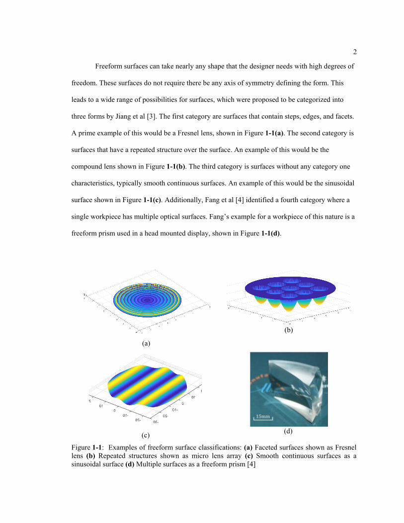
Figure 1-1: Examples of freeform surface classifications: (a) Faceted surfaces shown as Fresnel lens (b) Repeated structures shown as micro lens array (c) Smooth continuous surfaces as a sinusoidal surface (d) Multiple surfaces as a freeform prism [4] ....................... 2
Figure 1-2: Perspectives of (a) a normal motorcycle rearview mirror versus (b) a freeform surface motorcycle rearview mirror [11]. ................................................................. 4
Figure 1-3: Fast tool servo turning lathe configuration. ......................................................... 6
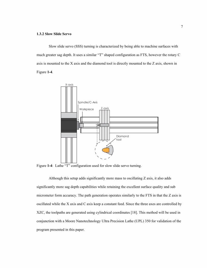
Figure 1-4: Lathe “T” configuration used for slow slide servo turning. ................................. 7
Figure 1-5: Diagram showing diamond turning workflow. .................................................... 9
Figure 2-1: Essential functions and workflow of a CAM program. ....................................... 12
Figure 2-2: Entire folder structure of MasterFlash with the core CAM functions highlighted in color... ............................................................................................................... 13
Figure 3-1: Relation between polar XCZ coordinates and cartesian xyz coordinates. ........... 17
Figure 3-2: Examples of Archimedean spirals using (a) constant angle and (b) constant arc length. Note that spacing has been exaggerated for easier viewing. .................................. 18
Figure 3-3: Example of how spacing increases for a traditional Archimedean spiral with respect to the angle of the surface[26] shown from (a) top view and (b) side view. ............... 20
Figure 3-4: Representation how the space spiral maintains even three dimensional spacing [26]. ............................................................................................................................. 21
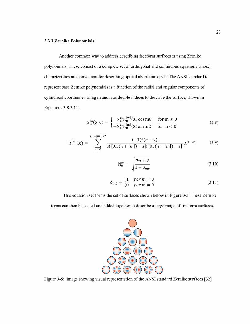
Figure 3-5: Image showing visual representation of the ANSI standard Zernike surfaces [32]. .......................................................................................................................................... 23
Figure 3-6: Representation of spiral being fit the surface to create the toolpath. ................... 25
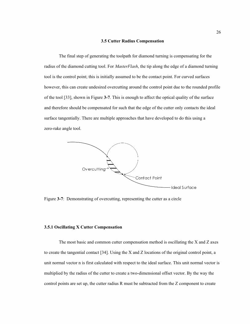
Figure 3-7: Demonstrating of overcutting, representing the cutter as a circle. ....................... 26
Figure 3-8: Cutter compensation using oscillating X and Z axes. .......................................... 27
Figure 3-9: Demonstration of steady X cutter compensation theory. ..................................... 29
Figure 3-10: Demonstration of steady X cutter compensation using clusters of test points. Cluster spacing has been exaggerated for easier viewing. ....................................................... 30
Figure 3-11: Visualization for the setup for Golden separation binary search. ...................... 32
Figure 3-12: Visualization for an iteration step in the Golden separation binary search. ....... 33

viii
Figure 4-1: MasterFlash coordinate set up visualization. ....................................................... 37
Figure 4-2: Visualization of the total offset to generate the base points. ................................ 38
Figure 4-3: Depiction of the different regions of the cutting algorithm implemented in MasterFlash. The blue shade represents the roughing material to remove and tan represents the finishing material to remove. (a) Cutting of the optional facing passes in the beginning with constant depth removal. (b) Cutting of the rough passes where the finish layer has begun to be reached and accounted for. (c) Nearing the end of the roughing passes. (d) Beginning the finishing passes. .............................................................. 43
Figure 5-1: Three-dimensional plot showing the complete toolpath for a pass. The green shows the entry portion of the path, the blue shows the cutting portion, the red shows the retraction portion. ..................................................................................................................... 49
Figure 5-2: Trajectory positions, velocities, and accelerations for the retraction path with the cutting path shown in blue and the retraction path shown in red. The graphs are split by (a) X axis (b) C axis (c) Z axis. .......................................................................................... 54-55
Figure 5-3: Trajectory positions, velocities, and accelerations for a roughing entry path with the cutting-portion shown in blue and the entry portion shown in green. The graphs are split by (a) X axis (b) C axis (c) Z axis. ............................................................................. 58-59
Figure 5-4: Trajectory positions, velocities, and accelerations for a finishing entry path with the cutting portion shown in blue and the entry portion shown in green. The graphs are split by (a) X axis (b) C axis (c) Z axis. ............................................................................. 60-61
Figure 5-5: Example excerpt of outputted G-code for G01 command from a roughing pass........................................................................................................................................... 66
Figure 6-1: Top and side views of the diamond cutter insert with the included angle, cutter radius, and clearance angle identified. ........................................................................... 70
Figure 6-2: Sectional curve breakdown to check the cutter radius. ........................................ 71
Figure 6-3: (a) The geometry chosen to find the points for circle fitting (b) Fitting a circle to three points using the double bisection method. ........................................................ 71-72
Figure 6-4: Cutter radius circles, shown in red, fit to a section curve shown in blue. ............ 72
Figure 6-5: Included angle related interference is highlghted in red. ..................................... 73
Figure 7-1: Depiction for centering the Z height of a diamond tool (a) too low and (b) too high [39]. ............................................................................................................................ 75
Figure 7-2: Depiction for centering the X height of a diamond tool (a) undercut center cylinder and (b) overcut characteristic “W” shape. ................................................................. 76

ix
Figure 7-3: MATLAB surface plots of each of the four surfaces used to test MasterFlash. Pictured are (a) 8-sided pyramid, (b) lens array (c) off axis paraboloid, and (d) dimpled curved surface. ..................................................................................................... 78-79
Figure 7-4: Pictures showing the final machined surfaces. (a)&(b) 8-sided pyramid (c)&(d) 2x2 micro lens array (e)&(f) dimpled surface. ........................................................... 80-81
x
LIST OF TABLES
Table 3-1: Table containing the information of the input arguments, output arguments, and any internal program variables accessed for fcn_ArchimedesSpriral. ...................... 19
Table 3-2: Table showing the relations between the program’s structure arrays and the local variables within fcn_ArchimedesSpiral. .................................................................. 20
Table 3-3: Table showing the modifiers to change within fcn_Zernike. ................................. 25
Table 3-4: Table containing the information of the input arguments, output arguments, and any internal program variables accessed for fcn_OscXCutterComp. ........................ 28
Table 3-5: Table showing the relations between the program’s structure arrays and the local variables within fcn_OscXCutterComp. .................................................................. 28
Table 3-6: Table containing the information of the input arguments, output arguments, and any internal program variables accessed for fcn_SteadyXCutterComp. .................... 30-31
Table 3-7: Table showing the relations between the program’s structure arrays and the local variables within the fcn_SteadyXCutterComp. ........................................................ 31
Table 3-8: Table containing the information of the input arguments, output arguments, and any internal program variables accessed for fcn_GoldenSteadyXCutterComp. ........ 34
Table 3-9: Table showing the relations between the program’s structure arrays and the local variables within the fcn_GoldenSteadyXCutterComp. ............................................ 34
Table 4-1: Table containing the information of the input arguments, output arguments, and any internal program variables accessed for fcn_MachiningSetup. .......................... 39-40
Table 4-2: Table showing the relations between the program’s structure arrays and the local variables within the fcn_MachiningSetup. .............................................................. 40
Table 4-3: Table containing the information of the input arguments, output arguments, and any internal program variables accessed for fcn_FinishingPasses. .......................... 41-42
Table 4-4: Table showing the relations between the program’s structure arrays and the local variables within the fcn_FinishingPasses. .............................................................. 42
Table 4-5: Table containing the information of the input arguments, output arguments, and any internal program variables accessed for fcn_RoughingPasses. .......................... 45
Table 4-6: Table showing the relations between the program’s structure arrays and the local variables within the fcn_RoughingPasses. .............................................................. 45
Table 5-1: Table containing the information of the input arguments, output arguments, and any internal program variables accessed for fcn_InverseTimeCalcs. ........................ 47-48

xi
Table 5-2: Table showing the relations between the program’s structure arrays and the local variables within fcn_InverseTimeCalcs. .................................................................. 50
Table 5-3: Table containing the information of the input arguments, output arguments, and any internal program variables accessed for fcn_Retraction. .................................... 54-55
Table 5-4: Table showing the relations between the program’s structure arrays and the local variables within fcn_Retraction. .............................................................................. 55
Table 5-5: Table containing the information of the input arguments, output arguments, and any internal program variables accessed for fcn_EntryPasses. ................................. 62-63
Table 5-6: Table showing the relations between the program’s structure arrays and the local variables within fcn_EntryPasses. ........................................................................... 63
Table 5-7: Table containing the information of the input arguments, output arguments, and any internal program variables accessed for fcn_NCFileWrite. ................................ 67-68
Table 5-8: Table showing the relations between the program’s structure arrays and the local variables within fcn_NCFileWrite. .......................................................................... 68

xii
ACKNOWLEDGEMENTS
First and foremost, I must express my deepest gratitude for the funding opportunity
available from the John Bruning Fellowship. It is thanks to this support that I have had the chance
to work, learn, and grow with the Machine Dynamics Research Lab. Dr. Bruning, also a Penn
State alumnus, is known for his research and philanthropy throughout his career within precision
engineering. It is thanks to individuals like Dr. Bruning that allow us to stand on the shoulders of
giants going forward.
I would also like to thank my research advisor Dr. Eric Marsh for his support and
guidance through my academic career. From my very first tour of Penn State before undergrad to
now, Dr. Marsh has inspired and made me proud to be an engineer.
I would also like to thank Dave Arneson and Byron Knapp from the Professional
Instruments Company for their contributions and moral support. Much of the equipment that
made this incredible opportunity possible was donated through them.
I would also like to thank Chris Morgan and Eric Alarie from Moore Nanotechnology for
their support and guidance through this process. Their expert knowledge was invaluable while
developing this program.
I also would like to thank the incredible group of friends I have been fortunate enough to
have developed here at Penn State. Your moral support and comradery made the long nights spent
in Reber that much more enjoyable. Finally, I would like to thank my parents for their love and
support through all these years. It is thanks to them I want to continue to be a better person and
work to my fullest potential.

1
Chapter 1
Introduction
Freeform surfaces can be described as high degree of freedom surfaces that do not require
any axes of symmetry. This freedom in design coupled with the capabilities of single point
diamond turning have proved to be extremely valuable in the optics industry finding applications
from imaging, lithography, space travel and beyond. These optics can lower the number of parts
needed for an assembly, decrease weight, and increase performance in optical systems. Slow slide
servo turning has shown to be a versatile way to machine a large variety of these freeform optics.
Through the years of development, there have been many methods created to generate the
toolpath for these surfaces.
1.1 Freeform Surfaces
Advances in manufacturing capabilities and complexity needed in machined surfaces
today have led to the need for freeform surfaces and the technology necessary to produce them.
Traditionally manufacturing has produced sphere shaped parts including flat surfaces, which are
just spheres of infinite radii. These spherical parts are rotationally symmetric and easy to produce;
however, the parts are not always able to satisfy all demands. Freeform surfaces have been
developed to improve aesthetic and functional possibilities over traditional manufactured parts
[1]. One of these possibilities that Medicus et al [2] notes is the ability to machine a complex
component to serve the same function as multiple traditionally manufactured parts, lowering
weight, space, and improving the performance.
2
Freeform surfaces can take nearly any shape that the designer needs with high degrees of
freedom. These surfaces do not require there be any axis of symmetry defining the form. This
leads to a wide range of possibilities for surfaces, which were proposed to be categorized into
three forms by Jiang et al [3]. The first category are surfaces that contain steps, edges, and facets.
A prime example of this would be a Fresnel lens, shown in Figure 1-1(a). The second category is
surfaces that have a repeated structure over the surface. An example of this would be the
compound lens shown in Figure 1-1(b). The third category is surfaces without any category one
characteristics, typically smooth continuous surfaces. An example of this would be the sinusoidal
surface shown in Figure 1-1(c). Additionally, Fang et al [4] identified a fourth category where a
single workpiece has multiple optical surfaces. Fang’s example for a workpiece of this nature is a
freeform prism used in a head mounted display, shown in Figure 1-1(d).
(a)
(b)
(c)
(d)
Figure 1-1: Examples of freeform surface classifications: (a) Faceted surfaces shown as Fresnel lens (b) Repeated structures shown as micro lens array (c) Smooth continuous surfaces as a sinusoidal surface (d) Multiple surfaces as a freeform prism [4]

3
1.2 Freeform Surface Applications
The large range of freedom and precision that is available through diamond machined
freeform surfaces leads to many applications where traditional manufacturing is either too costly
or not possible. Industries that have benefitted from this include aerospace, automobile, medical,
die and mold making, and the consumer sector [1]. The most common application within these
industries is optics. One of the earliest examples of using freeform optics is the Polaroid SX-70
camera [5], [6]. Its unique four bar linkage design and up to infinite focal range required the use
of two freeform optic pieces to correct a problem with the eye focus in the viewfinder [7]. Yi et al
[8] et al reported multiple modern applications of using freeform optics. In one example, a phase
plate modeled using a freeform surface was used for aberration correction within human eyes. In
another application Yi et al manufactured an Alvarez lens array using diamond turning [9]. An
Alvarez lens contains two bicubic phase profile lenses that enable correction of astigmatic
aberrations.
Chang et al [10] was able to successfully implement using freeform surfaces to improve
the rear-view mirror for a motorcycle. A traditional flat plane rear-view mirror had a 12˚ field of
view, which creates a blind spot for the rider. By implementing a freeform surface for the mirror,
the field of view was able to be increased to 52.7˚, eliminating the previous blind spot. . The field
of view change can be seen in Figure 1-2.

4
Hitachi [12] was able to greatly reduce the minimum distance needed for projectors using
a freeform optic assembly. Generally, projectors need a long clear distance in the range of several
meters to focus properly, which can create a large amount of dead space in a room. The
projection distance needed was able to be reduced to 47 cm using a freeform assembly. More
recently in 2020, Hembacher under Carl Zeiss applied for a patent [13] for a method that involves
producing freeform mirrors that can be used for either EUV or DUV microlithography, the
technology that produces computer chips.
The same applications that benefit from using freeform surfaces have high precision
requirements to function properly. These requirements include nanometric surface roughness and
sub micrometer form accuracy. Traditional machining methods are not able to produce this in a
single operation, needing expensive and time-consuming post processing operations such as
grinding after machining. Alternatively, diamond machining operations are capable to create
these high precision surfaces in one operation within these precise tolerances.
Figure 1-2: Perspectives of (a) a normal motorcycle rearview mirror versus (b) a freeform surface motorcycle rearview mirror [11].

5
1.3 Diamond Machining Methods
To manufacture these more complex surfaces, diamond machining methods were
introduced. These methods use high precision equipment that are capable of machining optic
quality surfaces directly without the need for other treatments. For usable materials, there are
limitations for what is considered diamond turnable. Technically any material can be diamond
turned, but some materials such as ferrous alloys wear away the diamond tool too quickly to be
used. Some of the materials that are diamond turnable include softer and more ductile materials
that are difficult to polish[14] such as oxygen free copper or Al6061 aluminum alloy, which are
convenient to use since they have good machinability[15]. Machines capable of producing these
surfaces generally require three degrees of freedom, but it is not uncommon for there to be up to
five. Some example machining processes capable of creating these surfaces that will not be
covered in detail here include ultra-precision milling, raster milling, ultra-precision grinding, and
diamond micro chiseling. These can generate freeform optical surfaces but are often niche and
contain limitations in either the capacity of surfaces possible or in extremely long machining
times[16]. Single point diamond turning has proved to be a fast and versatile process that can be
executed either as fast tool servo (FTS) and slow slide servo (SSS).
1.3.1 Fast Tool Servo
The FTS method is characterized by the ability to cut in the sag direction (along the Z
axis, perpendicular to the face of the part) at high frequencies[17]. An ultraprecision lathe set for
fast tool servo will have a control over the X and Z axes, which are set as perpendicular in a “T”
configuration with the Z axis pointing in parallel with the rotation axis of the spindle. The

6
diamond tool is attached to an additional lighter weight actuator known as Z’ axis capable of
short stroke lengths at high frequencies. Shown below in Figure 1-3.
The most common actuator is a piezo electric actuator capable of stroke lengths up to one
millimeter at frequencies up to 2kHz. For longer stroke lengths but slower response, the piezo
electric actuator can be replaced by a voice coil motor[4]. For the control process, the X axis
works from a constant feed working from the outside to the part center. The Z coordinate is then
determined from a combination of the X and rotation angle of the spindle, the C axis. This
method is ideal for generating optical surfaces with highly repeated microstructures, where the
fast responsiveness of the tool is well paired with the quickly repeating pattern of shallow depth.
However, that does point towards of the challenge of FTS: the capabilities of sag depth and
frequency will be inversely proportional, meaning an optimal solution may not always be
possible. In most cases the shallow sag depth will become the limiting factor of possible surfaces
[4].
Figure 1-3: Fast tool servo turning lathe configuration [4].
Z-axis
SpindleX-axis
Workpiece
Diamondtool
Z’-axis
Actuator
7
1.3.2 Slow Slide Servo
Slow slide servo (SSS) turning is characterized by being able to machine surfaces with
much greater sag depth. It uses a similar “T” shaped configuration as FTS, however the rotary C
axis is mounted to the X axis and the diamond tool is directly mounted to the Z axis, shown in
Figure 1-4.
Although this setup adds significantly more mass to oscillating Z axis, it also adds
significantly more sag depth capabilities while retaining the excellent surface quality and sub
micrometer form accuracy. The path generation operates similarly to the FTS in that the Z axis is
oscillated while the X axis and C axis keep a constant feed. Since the three axes are controlled by
XZC, the toolpaths are generated using cylindrical coordinates [18]. This method will be used in
conjunction with a Moore Nanotechnology Ultra Precision Lathe (UPL) 350 for validation of the
program presented in this paper.
Figure 1-4: Lathe “T” configuration used for slow slide servo turning.
Spindle/C-Axis
Diamondtool
X-axis
Z-axisWorkpiece

8
Capabilities of the Moore Nanotechnology UPL 350
The Moore-Nanotechnology UPL 350 follows the “T” configuration presented in Figure
1-4 in the slow slide servo section [19]. Its X and Z axes use linear brushless DC motors with a
resolution of .034 nanometers. The precision air spindle is equipped with a rotary optical encoder
with a resolution of 20,480,000 counters per revolution. All axes feature PID control with
feedforward compensation. Key precision machine tool features of the UPL-350 include high
structural loop stiffness and good damping properties [20]–[22].
1.4 Diamond Turning Workflow
Although there will be some minor variations, the general workflow for a diamond
turning operation can be seen below in Figure 1-5. First an optical surface as described above is
designed in an optical design package. The surface will typically be described by either a
mathematical function, such as a NURBS surface, or through using Zernike Polynomials. These
surface descriptions will be discussed in further detail in Chapter 3.3. These models of the
surfaces are then sent to a Computer Automated Machining (CAM) package to be processed into
G-code for machining.
First the CAM package uses the surface descriptions to calculate all the passes and cutter
location(CL) data points needed to machine the desired surface. The CL data is then transferred to
the package’s post processor that uses the desired machining parameters to convert the cutter
location data into the appropriate version of G-Code, the language used for computer numerical
control(CNC). The G-Code is analyzed and revised if necessary, and then sent to the machine,
which is an ultra-precision lathe for the case of diamond turning.

9
The lathe’s onboard controller then interprets the G-Code and converts it into commands
performed by the lathe, producing the diamond turned part. This part can then be precisely
scanned to reproduce the machined surface virtually. This can be fit to the original surface
functions and compared to potentially provide any feedback for the surface design or machining
parameters.
1.5 CAM Program Considerations
One of the complications that comes during this process is in the use of the CAM
package. Due to the need of programming with the synchronization of the linear axes with the
rotary C axis to create these freeform surfaces, many of the common commercially available
Figure 1-5: Diagram showing diamond turning workflow.
Cutter Locations G-Code
Revision
CAM Package
Freeform Surface Description
Optical Design Software
Controller MachinedPart
Ultra Precision Lathe
Measurement vs. Design
Metrology
Revision

10
CAM software are not able to generate the necessary G-Code. Generally, they have limited to no
C-Axis turning support. Additionally, as this technology has progressed, there have been may
different methods developed for various applications of diamond turning. Thus, for this Thesis a
modular program has been developed using MATLAB capable of producing the G-Code
necessary for diamond turning freeform optics using an adaptive framework capable of
supporting many diamond turning methods. The validity of the program was then tested using a
Moore Nanotechnology UPL 350.

Chapter 2
CAM Program Framework and Features
A key feature of the developed CAM program named MasterFlash, is its capability to
adapt to the different techniques used for diamond turning for path generation and post
processing. The way MasterFlash achieves this is through smart data storage and a multi-layered
code structure to allow modularity in function calls and appropriate data structures.
2.1 CAM Essential Functions Workflow
The better understand the need for modularity, the full requirements of a CAM program
for diamond turning will first be covered. The progression of essential functions is depicted
below in Figure 2-1. Note that each of these sections will be explored in further detail later
reviewing current methods and identifying which have been implemented into MasterFlash so far
and how they function. The first section of the process is toolpath generation, where the base
points of the toolpath along the desired surface are calculated. The machining parameters are used
to generate the control 2d spiral toolpath. This is then fit to desired surface to generate the control
points. Finally, due to the precision needed for freeform optics, the cutter radius must be
compensated for to avoid overcutting.
The next section is generating the actual cutter locations for turning from the control
points. First a coordinate system is established in the program relating the program to the
machining coordinate system. This is then used to shift the base points to be within a desired
machining coordinate frame. Following this, the roughing and finishing passes can be generated
from the base points using a cut algorithm. The feed rates for each pass can then be calculated

12
using pass locations and machining parameters. Finally, entry and exit paths of the cut can be
calculated and appended to each pass respectively creating the total paths.
The final section of the CAM program is the post processing of the total toolpaths. First,
the necessary safety lines and start up G-Code are written to an empty NC file. Then all the total
path data is converted into movement commands as G-code. These movement commands can
then all be combined and written into the NC file to be read by the lathe’s controller.
2.2 Core Modular Framework
For each of the sections and subsections presented above, there have been multiple
methods developed that have different advantages in different applications. To make a robust
program, each of the subsections needs to be easily modified and swapped out and data stored
tacitly. This is done using the layered code structure pictured in Figure 2-2, the core CAM
functions identified in 2.1 are highlighted in colored folders. The program was developed in a Git
Repository using the git-flow branching model to maintain version control, easily share with
Figure 2-1: Essential functions and workflow of a CAM program.
MachiningParameters
Spiral DriverPoints
SurfaceFitting
CutterCompensation
Toolpath GenerationCoordinate
Setup
PassCalculation
DetermineFeedrates
Cutter Location
Convert toG-Code
Write NCFile
NC File
Entry &Exit
Post Process

13
others, and maintain documentation of commits[23]. This code structure was inspired from the
FLagSHyP program developed by Bonet et al[24] at Cambridge University. FLagSHyP is a non-
linear finite element analysis MATLAB program that has similar modularity demand as
MasterFlash.
To begin a job, the user first creates a folder within the JobFolder directory. A copy of
the input script(script_MasterFlash.m), full code shown in Appendix A1, is placed in this folder
along with a function for the desired surface to be cut. These along with the other features of
MasterFlash use a specific naming convention to easily organize and identify the purpose of files,
Figure 2-2: Entire folder structure of MasterFlash with the core CAM functions highlighted in color
script_
fx
alg_
fxfx
fx
fcn_
fx
var_
fx
fx
fx
fx
fx
fx
fx
fx
fx
fx
fx
fx
.nc
Job
AlgorithmsFunctions
InternalVariables
NCFile
fx
srf_

14
hereby referred to as a file identifier. The first word of the name preceding the underscore
identifies the file program intent. In the case of the input script, the file identifier “script_” is
exclusively used. For the naming of the function describing the surface within a job folder, the
convention of using a file identifier of “srf_” has been adopted.
In the first section of the input script, the user interacts to record all the relevant
machining parameters needed for the program that are likely subject to change and select the
desired algorithm to be used. These parameters are stored in structure arrays to provide clarity of
data and maintain an ability to store varying amounts and types of data. MasterFlash uses four
structures including ROUGH and FINISH for the respective pass machining parameters, SETUP
for relevant details to tool and machine parameters, and POST for data used in post processing.
For any other remaining settings or parameters, MasterFlash also incorporates a “hidden” (in
reference to the input script) internal variable function(var_internal.m), full code show in
Appendix A2, that stores parameters that are not likely to be changed such as machine limits but
are referenced multiple times throughout the program. This creates a centralized repository of
program information that is easy to modify and access. In the second section of the input script,
the relevant sections of the program folder structure are added to the valid MATLAB path. In the
last section, the appropriate algorithm function is called and passed the structures and surface
function handle.
The algorithm scripts are identified with the file identifier “alg_”, which coordinate the
completion of the CAM process. Each algorithm will contain an appropriate sequential calling of
the functions stored in the Code folder to follow the CAM process presented in section 2.1. These
functions are named with the file identifier “fcn_”. The algorithm controls the passing of the
relevant fields of the data structures to the appropriate functions. As functions are called, they can
add classes to the original structures to provide a complete scope of data transformation through
the process. This is where the high degree of modularity is added into the program. The functions

15
being called within a given algorithm are easy to swap to provide a large layer of flexibility. For
example, if a user wants to examine the quality difference of a numerical steady X cutter
compensation and an implicit varying X cutter compensation, two identical algorithms can be
completed, only modifying the function called for cutter compensation to allow for a quick and
easy comparison. Within the algorithm, the last core CAM process that is called is the NC file
write function. This will create a text file in the same job folder as the input script that will
contain the NC program. The following sections will go further into detail for each of these steps
in the CAM process.

Chapter 3
Toolpath Generation
The first and most complex step in generating the G-Code for diamond turning is creating
the toolpath. First an Archimedean spiral is generated cutting from the outside of the workpiece to
the center to assign the X and C coordinates. This spiral is then fit to the desired surface to
determine Z coordinates. Due to the precision requirements of freeform optics, these cutter
positions will then need compensated for the cutter radius to avoid overcutting. Methods for
accomplishing these functions will be reviewed and identify which and how these methods have
been implemented into MasterFlash thus far.
3.1 Working in Cylindrical Coordinates
An immediate difference in programming for single point diamond turning compared to
traditional machining is in the coordinate systems used to define cutter locations. Ordinarily
cutter locations are given in cartesian coordinates of x and z, but diamond turning uses the
cylindrical coordinates of polar X representing the polar radius, C representing the angle, and Z
remaining the same[16]. The conversion between the two can be mathematically shown below
Equations 3.1-3.3 and visually in Figure 3-1, for clarity purposes within this paper, cartesian
coordinates will be set in lowercase and the polar in uppercase. Currently, all MasterFlash
algorithms require that the surface function have inputs of X and C and output Z.
X = x2 + y2 (3.1)
𝐶𝐶 = atan2(𝑦𝑦, 𝑥𝑥) (3.2)

17
Z = z (3.3)
3.2 Generating the Base Spiral
The first step in tool path generation is determining the X and C coordinates of the
control points using a spiral path, working from the edge of the workpiece to the origin at the
center [16]. For the variation of spiral to use, there are three methods proven through prior
examples that vary in the spacing used to generate the paths.
3.2.1 Archimedean Spirals
The first two methods are based around the sampling of an Archimedean spiral. This
parametric curve is generated by decreasing the X value starting from the radius of the workpiece
Figure 3-1: Relation between polar XCZ coordinates and cartesian xyz coordinates.

18
R by a constant federate fr inward as the angle C is increased by a constant spacing Δϴ. This can
be described by equations 3.4 and 3.5 below.
Ci = i ∗ Δθ (3.4)
Xi = R − fr ∗ Δθ ∗ i (3.5)
The first Archimedean spiral method uses constant arc length to discretize the spiral into
control points[24], [25]. This creates an even spacing across the entire workpiece between cutting
points and therefor creates a constant profile error from the discretization. This profile error
becomes proportional to the arc length chosen for the spiral. The drawback comes to a loss of
accuracy near the center, in which the second method of equal angle spacing spirals has an
advantage. Instead of chord length, the spiral is discretized according to a constant angle [26].
The center accuracy comes at a cost of varying profile error across the surface. An exaggerated
comparison of the two can be compared in below in Figure 3-2.
(a) (b)
Figure 3-2: Examples of Archimedean spirals using (a) constant angle and (b) constant arc length. Note that spacing has been exaggerated for easier viewing.

19
fcn_ArchimedesSpriral
[X_Theta] = fcn_ArchimedesSpiral(type,fr,res,r)
This function outputs a matrix containing the X and C values of the control points for the
driver spiral. The arguments used and their relation between the local variables and program
variables can be seen below in Tables 3-1 and 3-2. The full code can be seen in Appendix A-3.
The function operates by first calculating the number of points by finding the total length
of the pass using the radius and feed rate and then dividing it by the appropriate resolution. In the
second section the number of points is used to step through a for loop to calc the X and C points
of the spiral following the principles of equations 3.4 and 3.5. As a note, the constant arc length
has been developed to this point, but current algorithms are not set up to handle this spacing for
specific calculations further in the program.
Table 3-1: Table containing the information of the input arguments, output arguments, and any internal program variables accessed for fcn_ArchimedesSpriral
Input Arguments type - Spiral type selector Scalar Set as 1 for constant angle, 2 for constant arc length fr - X axis feed rate Scalar The constant x axis feed rate res - Spacing resolution for spiral Scalar Give degrees for type 1, or distance for type 2 r - Workpiece radius Scalar Radius of the workpiece being machined Output Arguments X_Theta - Control points Matrix Matrix containing the X and C coordinates of the control points

20
3.2.2 Space Archimedean Spiral
One form of spiral that has not been developed for the program yet but has shown to be
highly effective in certain applications is the use of a space Archimedean spiral proposed by
Gong et al [26]. This method has been shown to provide better resolution when dealing with
surfaces that have high slopes. In these steeper areas, the relative 3D spacing between successive
passes is proportional to the slope of the surface for the 2D Archimedean spiral, as shown in
Figure 3-3.
Table 3-2: Table showing the relations between the program’s structure arrays and the local variables within fcn_ArchimedesSpiral
MasterFlash Function Units ROUGH/FINISH.type → type [numerical]
ROUGH/FINISH.feedRate → fr [mm/rev] ROUGH/FINISH.res → res [degrees or mm]
SETUP.workpieceRadius → r [mm] ROUGH/FINISH.controlPoints ← X_Theta [mm,rad,mm]
(a)
(b)
Figure 3-3: Example of how spacing increases for a traditional Archimedean spiral with respect to the angle of the surface[26] shown from (a) top view and (b) side view.

21
The space Archimedean spiral instead parametrizes itself with respect to the X, C, and Z
coordinates. This allows the space spiral to be initially mapped to a generic surface of revolution
that best fits the desired surface to machine. This is done by starting with an initial Archimedean
spiral, then establishing a relationship that decreases the rate X is changed parametrically in
proportion to the slope of the surface, or the rate that Z is changing on the fitted surface of
revolution. This mapping can be seen in Figure 3-4. This keeps the spacing between the passes
within 3D space consistent, fixing the resolution disparity.
3.3 Surface Descriptions
Next the desired freeform surface needs to be described mathematically, of which there
have been several methods developed over the years [27]. The more basic surfaces can be
described using simple mathematical equations such as sinusoidal functions or polynomials.
Faceted surfaces remain still basic and can be described using step functions to model the
discontinuities. From there out, more complex mathematical models need to be used.
(a)
(b)
Figure 3-4: Representation how the space spiral maintains even three dimensional spacing [4].

22
3.3.1 Aspheric Surface
A very prominent surface used in the optics industry is the aspheric lens. This uses the
sag equation shown in Equation 3.6 [28], where the radius of curvature of the sphere is R and the
X coordinate represents the radius in cylindrical coordinates. The parameter P is equal to 1/R, K
is the conic constant, even numbered Ai are spheric deformation constants, and odd numbered Ai
are aspheric coefficients.
Z = CX2
1 + �1 − (K + 1)𝑃𝑃2X2+ A1X + A2X2 + A3X3 + ⋯+ AnXn (3.6)
3.3.2 NURBS Surfaces
A common way to address describing freeform surfaces is using Non-uniform rational
b-splines (NURBS) [25]. This provides a parametric description of a surface that is supported by
many CAD and optical design software. This allows a large range of freeform surfaces to be
described using NURBS including faceted edges and continuous surfaces [29], [30]. The
mathematical description of a NURBS surface S using spiral points Pi,j is presented below in
Equation 3.7. The surface is parametrized with respect to locations u and v and weighted using
the factors of wi,j and wk,l. Finally, the knot vectors Ni,p and Nk,p form the control points as the
basis functions.
S(u, v) = ��Ni,p(u)Nij,q(v)wi,j
∑ ∑ Nk,p(u)Nl,q(v)wk,lml=0
nk=0
m
j=0
Pi,j
n
i=0
(3.7)
23
3.3.3 Zernike Polynomials
Another common way to address describing freeform surfaces is using Zernike
polynomials. These consist of a complete set of orthogonal and continuous equations whose
characteristics are convenient for describing optical aberrations [31]. The ANSI standard to
represent base Zernike polynomials is a function of the radial and angular components of
cylindrical coordinates using m and n as double indices to describe the surface, shown in
Equations 3.8-3.11.
Znm(X, C) = �
NnmRn
|m|(X) cos mC for m ≥ 0−Nn
mRn|m|(X) sin mC for m < 0
(3.8)
Rn
|m|(𝑋𝑋) = �(−1)𝑠𝑠(𝑛𝑛 − 𝑠𝑠)!
𝑠𝑠! [0.5(𝑛𝑛 + |𝑚𝑚|) − 𝑠𝑠]! [05(𝑛𝑛 − |𝑚𝑚|) − 𝑠𝑠]!𝑋𝑋𝑛𝑛−2𝑠𝑠
(𝑛𝑛−|𝑚𝑚|)/2
𝑠𝑠=0
(3.9)
Nn
m = �2𝑛𝑛 + 2
1 + 𝛿𝛿𝑚𝑚0 (3.10)
𝛿𝛿𝑚𝑚0 = �1 𝑓𝑓𝑓𝑓𝑓𝑓 𝑚𝑚 = 00 𝑓𝑓𝑓𝑓𝑓𝑓 𝑚𝑚 ≠ 0 (3.11)
This equation set forms the set of surfaces shown below in Figure 3-5. These Zernike
terms can then be scaled and added together to describe a large range of freeform surfaces.
Figure 3-5: Image showing visual representation of the ANSI standard Zernike surfaces [32].

24
fcn_Zernike
Z = fcn_Zernike(p,theta)
The ability to use Zernike functions has been implemented into MasterFlash through
fcn_Zernike located within the directory SurfaceEquations. The full code for this can be seen in
Appendix A-4. For convenience, this function also references fcn_ANSIorder shown in Appendix
A-5, which must be in the same folder. The ANSI function is used as a convenient way of calling
the m and n values within the Zernike function within a repeated loop. Although these two can be
used as a standalone surface file for the program, due to the use of factorials, for speed purposes it
is best used to generate an equation for a srf_ file using symbolic inputs of p and theta. The
symbolic output is then used to create its own srf_ file to be used in the Job folder for much
higher speeds.
There are modifiers within the function that need to be changed to generate the correct
equation for the desired surface shown in Table 3-3. First, the function starts with a 36x1 matrix
of zeroes for the coeff variable, for each of the currently supported ANSI Zernike terms. The user
inputs the desired coefficients to be multiplied to the respective Zernike terms that are intended to
be used. Any terms with zero will be ignored. The other modifier that needs adjusted is p_max
needs to be set as the radius of the workpiece.
The calculations begin by normalizing the input p to the p_max value. The function then
steps a loop through the coefficient matrix that executes whenever a value is non-zero. For
execution, Equations 3.8-3.11 are used to create the base Zernike terms, the term is multiplied by
the corresponding coefficient, and then added to the overall equation.

25
3.4 Mapping Spiral to Surface
The next step in the toolpath generation progress is to map the spiral control points to the
desired surface, creating three-dimensional control points for the surface. This is done
straightforwardly with the prior setup through the algorithm passing the X and C control points
generated from the spiral function into the desired surface function. The resulting vector of Z
values is appended as the third column to the ROUGH/FINISH.controlPoints matrix. The result is
a nx3 matrix containing the values of all three cylindrical dimensions for the control points
describing the toolpath to cut the surface. A visualization of this can be seen below in Figure 3-6.
Table 3-3: Table showing the modifiers to change within fcn_Zernike
Modifier Effect coeff Determines the Zernike terms used and scales them
p_max Normalizes the radius terms to the workpiece radius
Figure 3-6: Representation of spiral being fit the surface to create the toolpath.
26
3.5 Cutter Radius Compensation
The final step of generating the toolpath for diamond turning is compensating for the
radius of the diamond cutting tool. For MasterFlash, the tip along the edge of a diamond turning
tool is the control point; this is initially assumed to be the contact point. For curved surfaces
however, this can create undesired overcutting around the control point due to the rounded profile
of the tool [33], shown in Figure 3-7. This is enough to affect the optical quality of the surface
and therefore should be compensated for such that the edge of the cutter only contacts the ideal
surface tangentially. There are multiple approaches that have developed to do this using a
zero-rake angle tool.
3.5.1 Oscillating X Cutter Compensation
The most basic and common cutter compensation method is oscillating the X and Z axes
to create the tangential contact [34]. Using the X and Z locations of the original control point, a
unit normal vector n is first calculated with respect to the ideal surface. This unit normal vector is
multiplied by the radius of the cutter to create a two-dimensional offset vector. By the way the
control points are set up, the cutter radius R must be subtracted from the Z component to create
Figure 3-7: Demonstrating of overcutting, representing the cutter as a circle
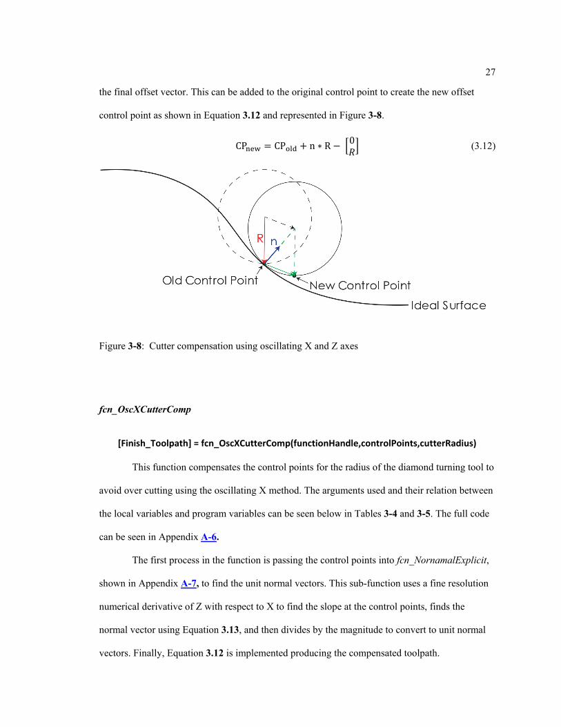
27
the final offset vector. This can be added to the original control point to create the new offset
control point as shown in Equation 3.12 and represented in Figure 3-8.
fcn_OscXCutterComp
[Finish_Toolpath] = fcn_OscXCutterComp(functionHandle,controlPoints,cutterRadius)
This function compensates the control points for the radius of the diamond turning tool to
avoid over cutting using the oscillating X method. The arguments used and their relation between
the local variables and program variables can be seen below in Tables 3-4 and 3-5. The full code
can be seen in Appendix A-6.
The first process in the function is passing the control points into fcn_NornamalExplicit,
shown in Appendix A-7, to find the unit normal vectors. This sub-function uses a fine resolution
numerical derivative of Z with respect to X to find the slope at the control points, finds the
normal vector using Equation 3.13, and then divides by the magnitude to convert to unit normal
vectors. Finally, Equation 3.12 is implemented producing the compensated toolpath.
CPnew = CPold + n ∗ R − �0𝑅𝑅� (3.12)
Figure 3-8: Cutter compensation using oscillating X and Z axes

28
𝑁𝑁𝑓𝑓𝑓𝑓𝑚𝑚𝑁𝑁𝑁𝑁 = �−𝑠𝑠𝑁𝑁𝑓𝑓𝑠𝑠𝑠𝑠1� (3.13)
3.5.2 Steady X Cutter Compensation
The other way to compensate for the cutter with a zero-degree rake angle is to only offset
the cutter in the Z direction [34]. Ping et al noted there are two advantages to using this method.
First, using derivatives near faceted edges can create numerical instability that could cause errors.
Second is if the surface is complex enough, the x axis compensation may create too high of a
Table 3-4: Table containing the information of the input arguments, output arguments, and any internal program variables accessed for fcn_OscXCutterComp
Input Arguments functionHandle - Surface function call Handle MATLAB handle used to call the surface function controlPoints - Cutting path control points Matrix Non-compensated matrix of control points cutterRadius - Radius of cutting tool Scalar Radius of the diamond turning tool Output Arguments Finish_Toolpath - Control points of path Matrix Matrix containing the compensated values of the control points
Table 3-5: Table showing the relations between the program’s structure arrays and the local variables within fcn_OscXCutterComp
MasterFlash Function Units
surfaceFcn → functionHandle [handle] ROUGH/FINISH.controlPoints → controlPoints [mm,rad,mm]
SETUP.cutterRadius → cutterRadius [mm] ROUGH/FINISH.controlPoints ← Finish_Toolpath [mm,rad,mm]

29
frequency to execute due to the lower frequency response of the X-axis. To employ the steady X
method, the cutter edge profile positioned at the control point and surface profile are compared to
find the greatest negative vertical difference between the profiles. By adding the greatest
difference between the profiles to the Z coordinate of the control point, it will create the desired
tangential cutter contact, shown in Figure 3-9. There are two approaches to implement this
constant X cutter compensation reviewed and implemented into the MasterFlash program.
fcn_SteadyXCutterComp
[FinishToolpath] = fcn_SteadyXCutterComp(functionHandle,controlPoints, cutterRadius,includedAngle)
This function compensates the control points for the radius of the diamond turning tool to
avoid over cutting using a brute force steady X method. The arguments used and their relation
between the local variables and program variables can be seen below in Tables 3-6 and 3-7. The
full code can be seen in Appendix A-8.
This first approach creates two localized cluster of points around each control point in the
XZ plane. These clusters of points use a fine resolution of consistent displacements along the X
Figure 3-9: Demonstration of steady X cutter compensation theory

30
axis in the positive and negative direction from the central control point to edges of the cutter
nose. The two clusters are then mapped to the cutter edge profile and the surface profile
respectively and subtracted to compare displacements. The greatest negative vertical
displacement is added to the control points’ Z component to compensate for the cutter radius,
depicted in Figure 3-10.
Figure 3-10: Demonstration of steady X cutter compensation using clusters of test points. Cluster spacing has been exaggerated for easier viewing.
Table 3-6: Table containing the information of the input arguments, output arguments, and any internal program variables accessed for fcn_SteadyXCutterComp
Input Arguments functionHandle - Surface function call Handle MATLAB handle used to call the surface function controlPoints - Cutting path control points Matrix Non-compensated matrix of control points cutterRadius - Radius of cutting tool Scalar Radius of the diamond turning tool includedAngle - Included angle of tool Scalar Included angle of diamond turning tool

31
3.5.3 Golden Point Separation Steady X Compensation
Although the brute force method presented above will return the correct compensation
relative to the resolution needed, it can take a large amount of computation time to complete. Ping
et al [35] proposed using a binary search method using the golden point separation to optimize the
process to run faster. To begin the process, consider two functions of f(x) representing the desired
surface and h(x) representing the profile of the diamond cutting tool. A third equation is created
combining the subtraction of the two to create a function shown in Equation 3.14 representing the
difference of the profiles, g(x).
g(x) = f(x) – h(x) (3.14)
The algorithm is appropriate to use since the g(x) function is guaranteed to be unimodal,
or having only one maximum value [36]. This is because the cutter radius should be smaller than
any concave radius of curvature on the surface to prevent interference. The algorithm begins by
defining the minimum and maximum search bounds as xmin and xmax respectively. The initial
Output Arguments Finish_Toolpath - Control points of path Matrix Matrix containing the compensated values of the control points
Table 3-7: Table showing the relations between the program’s structure arrays and the local variables within the fcn_SteadyXCutterComp
MasterFlash Function Units
surfaceFcn → functionHandle [handle] ROUGH/FINISH.controlPoints → controlPoints [mm,rad,mm]
SETUP.cutterRadius → cutterRadius [mm] SETUP.includedAngle → includedAngle [degrees]
ROUGH/FINISH.controlPoints ← Finish_Toolpath [mm,rad,mm]

32
values of this in context to the cutter compensation will be the edges of the circular portion of the
cutter edge. Next, two inner test positions x0 and x1 will be chosen using a spacing parameter G
derived from the inverse of golden number φ, shown in Equations 3.15-3.17. These inner test
positions are then evaluated in the function g(x) to produce the values v0 and v1. A visual
representation of this setup can be seen in Figure 3-11.
G =
1φ
= √5 − 1
2 ≈ 0.618 (3.15)
x0 = xmin + (1 − G) ∗ (xmax − xmin ) (3.16)
x1 = xmin + G ∗ (xmax − xmin ) (3.17)
These two inner test values are then compared to determine the next iteration procedure.
If v0≤v1, the next iteration will let the new xmin be equal to the old x0 and the new x0 and v0 are set
equal to the old x1 and v1. Thanks to the proportions from using the golden number, only x1 and
v1 need to be recalculated using the same relations since the proportions are maintained through
each iteration. Similarly, if v0≥v1, the next iteration will set the new xmax equal to the old x1 and
the new x1 and v1 are set to the old x0 and v0. Then only x0 and v0 need to be recalculated. A
visualization of this process can be seen below in Figure 3-12. This iteration process is repeated
until the inner test values are within a desired resolution and v0 is used as the displacement the
Figure 3-11: Visualization for the setup for Golden separation binary search.
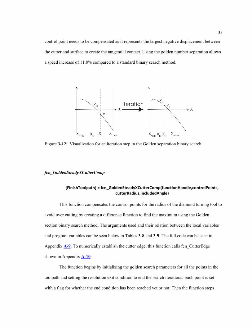
33
control point needs to be compensated as it represents the largest negative displacement between
the cutter and surface to create the tangential contact. Using the golden number separation allows
a speed increase of 11.8% compared to a standard binary search method.
fcn_GoldenSteadyXCutterComp
[FinishToolpath] = fcn_GoldenSteadyXCutterComp(functionHandle,controlPoints, cutterRadius,includedAngle)
This function compensates the control points for the radius of the diamond turning tool to
avoid over cutting by creating a difference function to find the maximum using the Golden
section binary search method. The arguments used and their relation between the local variables
and program variables can be seen below in Tables 3-8 and 3-9. The full code can be seen in
Appendix A-9. To numerically establish the cutter edge, this function calls fcn_CutterEdge
shown in Appendix A-10.
The function begins by initializing the golden search parameters for all the points in the
toolpath and setting the resolution exit condition to end the search iterations. Each point is set
with a flag for whether the end condition has been reached yet or not. Then the function steps
Figure 3-12: Visualization for an iteration step in the Golden separation binary search.

34
through iterations performing the golden binary search method on every point that still has not
reached end condition. This loop will continue until every single point has reached convergence.
Finally, the offset will be added to the control points Z value and outputted.
Table 3-8: Table containing the information of the input arguments, output arguments, and any internal program variables accessed for fcn_GoldenSteadyXCutterComp
Input Arguments functionHandle - Surface function call Handle MATLAB handle used to call the surface function controlPoints - Cutting path control points Matrix Non-compensated matrix of control points cutterRadius - Radius of cutting tool Scalar Radius of the diamond turning tool includedAngle - Included angle of tool Scalar Included angle of diamond turning tool Output Arguments Finish_Toolpath - Control points of path Matrix Matrix containing the compensated values of the control points
Table 3-9: Table showing the relations between the program’s structure arrays and the local variables within the fcn_GoldenSteadyXCutterComp
MasterFlash Function Units
functionHandle → functionHandle [handle] ROUGH/FINISH.controlPoints → controlPoints [mm,rad,mm]
SETUP.cutterRadius → cutterRadius [mm] SETUP.includedAngle → includedAngle [degrees]
ROUGH/FINISH.controlPoints ← Finish_Toolpath [mm,rad,mm]

35
3.6 Toolpath Generation Summary
The many methods used in single point diamond turning toolpath generation have been
investigated and the features that have been implemented as possibilities into MasterFlash were
reviewed. The creation of the control spiral, surface representations, and cutter compensations all
showed high degrees of variability that are capable of being handled by MasterFlash. It is
common practice to have different machining parameters between the rough and finish passes in
turning to save time and create the higher resolution only when necessary. MasterFlash will go
through the toolpath generation process twice to maintain a set of rough and finish control points
to be turned into cutter location data. These control points represent the exact same surface, they
just vary in resolution.
Chapter 4
Calculating Cutter Location Data
Once the rough and finish control points have been generated, the next step is to convert
this data into cutter locations to be post processed. First the machine coordinates relative to the
control points must be established. Then a cutting algorithm needs to be implemented to calculate
the number of passes required and determine the coordinates of all the cutter locations within
these passes.
4.1 Coordinate System Setup
For machining, there are a variety of coordinate frames available that can be used when
specifying position. The base coordinates are the absolute machine coordinates that are generated
whenever the machine has been homed; however, this is not convenient to use when programing
since the part zero will be different nearly every time. It is much more convenient to use a work
coordinate offset from the absolute machine coordinates that lines up with the part zero [18]. In
MasterFlash the chosen work coordinate system is flexible, but the default assumption is the
operator is using the G54 work coordinate system. In the calculations MasterFlash assumes the
work coordinate origin is set at part zero, which for diamond turning is on the face at the center of
the of the workpiece, and the work coordinate refers to the location of the front tip of the cutter,
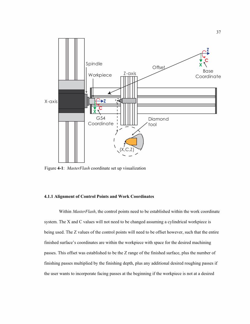
as shown in Figure 4-1. For example, the cutter would be at work coordinate zero at the end of a
facing pass when the cutter is still just in contact with the face at the center of the workpiece.
37
4.1.1 Alignment of Control Points and Work Coordinates
Within MasterFlash, the control points need to be established within the work coordinate
system. The X and C values will not need to be changed assuming a cylindrical workpiece is
being used. The Z values of the control points will need to be offset however, such that the entire
finished surface’s coordinates are within the workpiece with space for the desired machining
passes. This offset was established to be the Z range of the finished surface, plus the number of
finishing passes multiplied by the finishing depth, plus any additional desired roughing passes if
the user wants to incorporate facing passes at the beginning if the workpiece is not at a desired
Figure 4-1: MasterFlash coordinate set up visualization
Spindle
Diamondtool
X-axis
Z-axisWorkpiece
Z
XC
G54Coordinate
(X,C,Z)
Z
XC
BaseCoordinate
Offset

38
starting quality. The established base points represent the coordinates of the final turned surface.
A depiction of this offset can be seen in Figure 4-2.
fcn_MachiningSetup
[FinishBase,RoughBase,offset] = fcn_MachiningSetup(finishControlPoints,roughControlPoints, roughDepth,finishDepth,finishPasses)
This function completes the offsetting of the base control points in the Z direction to
ensure the coordinates are proper with respect to the workpiece. The arguments used and their
relation between the local variables and program variables can be seen below in Tables 4-1 and
4-2. The full code can be seen in Appendix A-11.
Figure 4-2: Visualization of the total offset to generate the base points.
Z
XC
Surface ZRange
AdditionalFacingPasses
TotalOffset
FinishingPasses

39
The program begins by setting the maximum Z coordinate within the finish control points
as the starting offset distance. By using the maximum for the offset, the surface function can be
positioned anywhere within the Z space and still be positioned correctly for machining with the
highest point being located at part zero. Additional offsets are then added for the finishing passes
and initial facing passes. This offset is then subtracted from the control points’ Z coordinates to
generate the base points for the cutting calculations.
Table 4-1: Table containing the information of the input arguments, output arguments, and any internal program variables accessed for fcn_MachiningSetup
Input Arguments finishControlPoints - Control points of finishing path Matrix Matrix containing the compensated values of the finish control points roughControlPoints - Control points of roughing path Matrix Matrix containing the compensated values of the rough control points roughDepth - Roughing depth Scalar Height to be used for roughing passes finishDepth - Finishing depth Scalar Height to be used for finishing passes finishPasses - Finishing Passes Scalar Total number of desired finishing passes roughPasses - Roughing Passes Scalar Total number of desired roughing passes Output Arguments FinishBase - Finishing base coordinates Matrix Matrix containing the correct offset coordinates of the finishing base points RoughBase - Roughing base coordinates Matrix Matrix containing the correct offset coordinates of the roughing base points

40
4.2 Cutting Pass Calculations
The next step is to calculate the cutting passes from the base data to generate all the
necessary cutter locations and passes to turn the desired surface. This was done by implementing
rough and finish cutting algorithms separately as they will operate on different principles.
4.2.1 Finishing Pass Calculations
The more straightforward passes to calculate from the base point data is the finishing
passes. The base point data already captures the correct X and C coordinates, the Z coordinates
just need a single uniform offset for each pass. The program begins a for loop for the designated
number of finishing passes desired. The first offset is the total number of finish passes multiplied
offset - Offset for the finishing boundary layer Scalar Finishing boundary layer offset used later in entry path generation
Table 4-2: Table showing the relations between the program’s structure arrays and the local variables within the fcn_MachiningSetup
MasterFlash Function Units
FINISH.controlPoints → finishControlPoints [mm,rad,mm] ROUGH.controlPoints → roughControlPoints [mm,rad,mm]
ROUGH.depth → roughDepth [mm] FINISH.depth → finishDepth [mm] FINISH.passes → finishPasses [passes] ROUGH.passes → roughPasses [passes]
FINISH.base ← FinishBase [mm,rad,mm] ROUGH.base ← RoughBase [mm,rad,mm]
offset ← offset [mm]

41
by the finish depth. Each subsequent pass’s offset will decrease by the finish depth until the final
pass is the finish base coordinates. This process is represented in Equations 4.1-4.4.
finishPass(i) = finishBase + offset(i) (4.1)
offset(1) = finishDepth ∗ finishPasses (4.2)
offset(i) = offset(1) − i ∗ finishDepth (4.3)
offset(end) = 0 (4.4)
fcn_FinishingPasses
[FinishToolpaths] = fcn_FinishingPasses(finishBase,finishDepth,finishPasses)
This function adds the respective offsets to the finish base points to create the coordinates
for the finishing passes. The arguments used and their relation between the local variables and
program variables can be seen below in Tables 4-3 and 4-4. The full code can be seen in
Appendix A-12.
This function operates by following the principles presented in Equations 4.1-4.4. The
paths are output using a 3D matrix to contain all path information.
Table 4-3: Table containing the information of the input arguments, output arguments, and any internal program variables accessed for fcn_FinishingPasses
Input Arguments finishBase - Finishing base coordinates Matrix Matrix containing the correct offset coordinates of the finishing base points finishDepth - Finishing depth Scalar Height to be used for finishing passes finishPasses - Finishing Passes Scalar Total number of desired finishing passes

42
4.2.2 Roughing Pass Calculations
The purpose of roughing passes is to quickly remove material such that an even thickness
layer of material remains for the finish layer(s) to complete the diamond turning process. Starting
from a flat face and ending in an any shaped surface means there will inherently be a varying
depth across the surface to rough cut out. MasterFlash uses an algorithm shown in Figure 4-3 to
accomplish these functions. Referring to the figure, the purpose of roughing is to machine down
the blue layer representing the material to be rough cut to the tan layer that represents the material
to be removed in finishing passes. First the maximum depth of the roughing passes required is
calculated by adding the room needed for finishing passes by multiplying the finish depth and
finish passes, to the lowest Z coordinate in the finish base coordinates. The finish base
coordinates are used over the rough base coordinates for the highest precision in calculations.
This depth is then divided by the depth of the roughing passes and rounded up to the nearest
Output Arguments FinishToolpaths - Finishing toolpath coordinates 3-D Matrix Complete set of finishing cutting path coordinates
Table 4-4: Table showing the relations between the program’s structure arrays and the local variables within the fcn_FinishingPasses
MasterFlash Function Units
FINISH.base → finishBase [mm,rad,mm] FINISH.depth → finishDepth [mm] FINISH.passes → finishPasses [passes]
FINISH.toolPaths ← FinishToolpath [mm,rad,mm,pass]
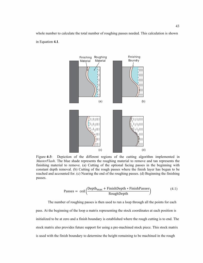
43
whole number to calculate the total number of roughing passes needed. This calculation is shown
in Equation 4.1.
Passes = ceil �
Depthmax + FinishDepth ∗ FinishPassesRoughDepth
� (4.1)
The number of roughing passes is then used to run a loop through all the points for each
pass. At the beginning of the loop a matrix representing the stock coordinates at each position is
initialized to be at zero and a finish boundary is established where the rough cutting is to end. The
stock matrix also provides future support for using a pre-machined stock piece. This stock matrix
is used with the finish boundary to determine the height remaining to be machined in the rough
Figure 4-3: Depiction of the different regions of the cutting algorithm implemented in MasterFlash. The blue shade represents the roughing material to remove and tan represents the finishing material to remove. (a) Cutting of the optional facing passes in the beginning with constant depth removal. (b) Cutting of the rough passes where the finish layer has begun to be reached and accounted for. (c) Nearing the end of the roughing passes. (d) Beginning the finishing passes.
(a)
(c)
(b)
(d)
Roughing Material
Finishing Material
Finishing Boundry

44
cutting process for each pass. As the loop iterates, all the points of a particular pass are evaluated
for three actions that could possibly partake. If the height remaining is greater than the roughing
layer height, the Z coordinate is decreased by the full roughing height. If the height remaining is
less than the rouging height but not zero, the Z coordinate is set to the height of the finishing
boundary. Finally, if the height remaining is zero, the Z coordinate remains at the finishing
boundary. Using the equation presented for the calculations for the number of roughing passes
needed, the final roughing pass will cut along the finish boundary. Once all the cutter locations
have been calculated, the cutter location data can be sent to post processing.
fcn_RoughingPasses
[RoughPasses,passes] = fcn_RoughingPasses(roughDepth,finishDepth, finishBase,finishPasses,roughBase)
This function runs through the roughing pass calculations to generate the complete set of
coordinates for the roughing passes. The arguments used and their relation between the local
variables and program variables can be seen below in Tables 4-5 and 4-6. The full code can be
seen in Appendix A-13.
The calculations follow the algorithm presented above. First the number of passes is
calculated using a finishing boundary and the stock variable is initialized. Then each pass is
stepped through for which the three cutting options for each point are decided by a call to the
subfunction fcn_CutCalc shown in full in Appendix A-14, updating the stock with each pass until
every pass has been calculated.

45
Table 4-5: Table containing the information of the input arguments, output arguments, and any internal program variables accessed for fcn_RoughingPasses
Input Arguments roughDepth - Roughing depth Scalar Height to be used for roughing passes finishDepth - Finishing depth Scalar Height to be used for finishing passes finishBase - Finishing base coordinates Matrix Matrix containing the correct offset coordinates of the finishing base points finishPasses - Finishing Passes Scalar Total number of desired finishing passes roughBase - Roughing base coordinates Matrix Matrix containing the correct offset coordinates of the roughing base points Output Arguments RoughToolpaths - Finishing toolpath coordinates 3-D Matrix Complete set of finishing cutting path coordinates passes - Number of roughing passes Scalar Calculated number of roughing passes
Table 4-6: Table showing the relations between the program’s structure arrays and the local variables within the fcn_RoughingPasses
MasterFlash Function Units
ROUGH.depth → roughDepth [mm] FINISH.depth → finishDepth [mm] FINISH.base → finishBase [mm,rad,mm]
FINISH.passes → finishPasses [passes] ROUGH.base → roughBase [mm,rad,mm]
ROUGH.toolPaths ← RoughPasses [mm,rad,mm,pass] ROUGH.passes ← passes [passes]

Chapter 5
Post Processing
After the cutter locations have been calculated for all rough and finish passes, the
locations need to be processed and converted into G-code to be run by the machine. First the feed
rates need to be calculated, then entry and exit path cutter locations need calculated, and finally
all the paths assembled and written to a NC file.
5.1 Inverse Time Calculations
After determining all the locations, the feeds need to be implemented to the cutting
passes. For slow slide servo execution, a common way to implement this is through using G93
inverse time mode [37]. A modal feed rate is specified that represents the time the move takes to
execute. The use of the constant angle Archimedean spiral works extremely well in conjunction
with this mode because it causes the cutting to happen under a constant spindle speed and
constant X axis feed, only the Z axis oscillates accordingly.
The initial feed rates are calculated by dividing the angular spacing by the desired spindle
speed to produce the time that would be required to make the move. This is rounded to the nearest
millisecond, with a lower limit of one millisecond due to the controller’s max block read rate
being 1kHz. This initial feed rate is used to calculate the velocities and accelerations of the Z
axis. If the values exceed the desired path parameters or machine limits, the feed rates will be
adjusted accordingly to stay within the path limits.

47
fcn_InverseTimeCalcs
[FeedRate] = fcn_InverseTimeCalcs(spindleSpeed,toolPaths)
The function outputs a nx1xm matrix containing the inverse time feed rates that is
appended as a fourth column to the toolpaths. The arguments used and their relation between the
local variables and program variables can be seen below in Tables 5-1 and 5-2. The full code can
be seen in Appendix A-15.
The function calculates the initial feed rate by dividing the angular spacing by the desired
spindle speed, with the smallest value possible being one millisecond. The maximum value of
each pass is used for the whole pass. A loop then runs through each pass calculating and adjusting
for crossing any limits in the Z travel for speed and acceleration. The final values for the feed rate
of every cutter location are rounded up to the nearest millisecond and outputted as a three-
dimensional matrix.
Table 5-1: Table containing the information of the input arguments, output arguments, and any internal program variables accessed for fcn_InverseTimeCalcs
Input Arguments spindleSpeed - Desired spindle speed while machining Scalar Desired spindle speed to be used while cutting. Must be given as a scalar toolPaths - Cutter locations of machining passes 3-D Matrix
3-Dimensional matrix that contains all the cutter locations for either the roughing or finishing passes. Output Arguments FeedRate - Inverse time rate feed rates for passes 3-D Matrix
3-Dimensional matrix that contains all the inverse time feed rates for each inputted cutter location Internal Variables Called maxSpeed - Maximum linear travel speed Scalar |4 m/min (default) Machine limit for linear travel speed
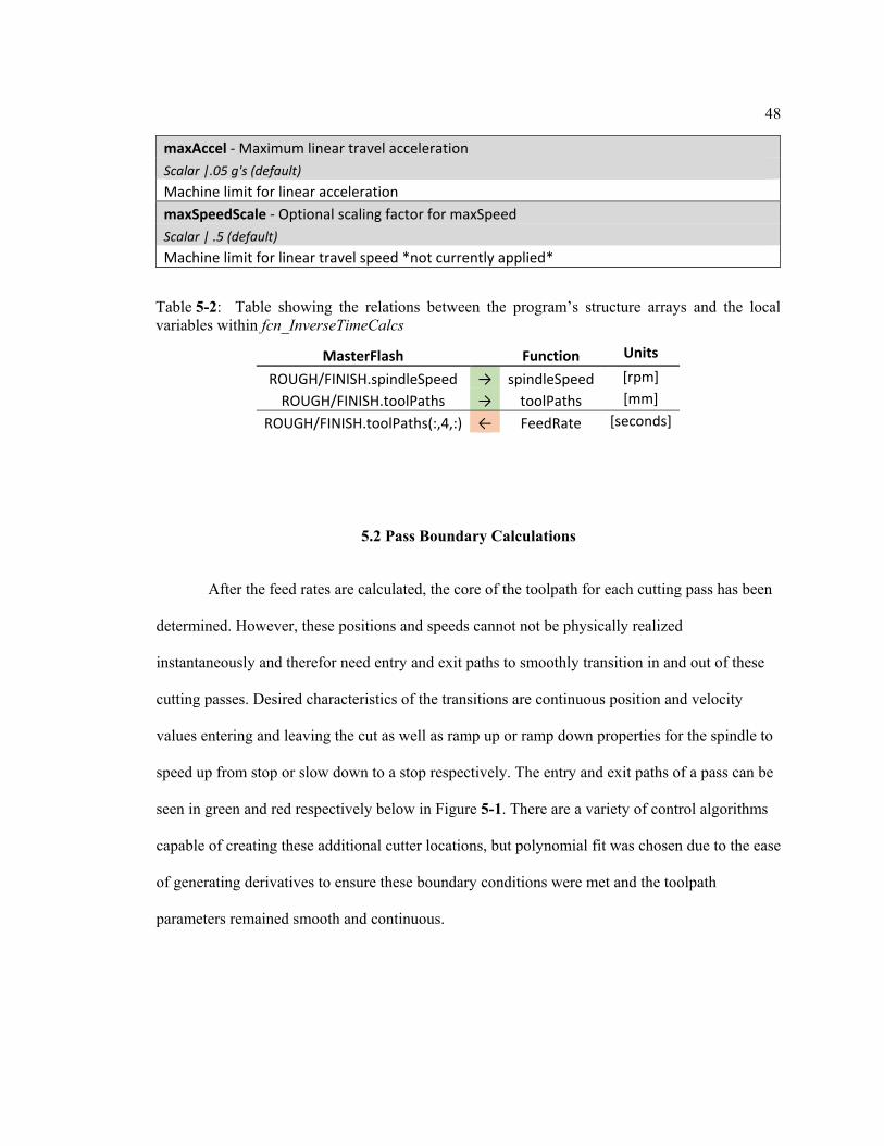
48
5.2 Pass Boundary Calculations
After the feed rates are calculated, the core of the toolpath for each cutting pass has been
determined. However, these positions and speeds cannot not be physically realized
instantaneously and therefor need entry and exit paths to smoothly transition in and out of these
cutting passes. Desired characteristics of the transitions are continuous position and velocity
values entering and leaving the cut as well as ramp up or ramp down properties for the spindle to
speed up from stop or slow down to a stop respectively. The entry and exit paths of a pass can be
seen in green and red respectively below in Figure 5-1. There are a variety of control algorithms
capable of creating these additional cutter locations, but polynomial fit was chosen due to the ease
of generating derivatives to ensure these boundary conditions were met and the toolpath
parameters remained smooth and continuous.
maxAccel - Maximum linear travel acceleration Scalar |.05 g's (default) Machine limit for linear acceleration maxSpeedScale - Optional scaling factor for maxSpeed Scalar | .5 (default) Machine limit for linear travel speed *not currently applied*
Table 5-2: Table showing the relations between the program’s structure arrays and the local variables within fcn_InverseTimeCalcs
MasterFlash Function Units
ROUGH/FINISH.spindleSpeed → spindleSpeed [rpm] ROUGH/FINISH.toolPaths → toolPaths [mm]
ROUGH/FINISH.toolPaths(:,4,:) ← FeedRate [seconds]

49
5.2.1 Retraction Path Generation
The retraction path will be appended to the end of the cutting toolpath to retract the cutter
tool in the Z direction to the retract height from the final cutting point while smoothly bringing
the spindle to a stop. Since the X axis should already be stopped at the center and be unchanged,
only the C and Z axes require the polynomial fit.
The initial boundary conditions for the Z polynomial are the location and velocity must
be continuous with the cutting path. The final boundary conditions for the Z polynomial are the Z
location is equal to the retract height and the velocity is zero. Having four boundary conditions
means the path can be generated using a generic third order polynomial as a function of time
shown in Equation 5.1 with the boundary conditions shown in Equations 5.2-5.5.
Z(t) = At3 + Bt2 + Dt + E (5.1)
Z(0) = Z0 (5.2)
Figure 5-1: Three-dimensional plot showing the complete toolpath for a pass. The green shows the entry portion of the path, the blue shows the cutting portion, the red shows the retraction portion.
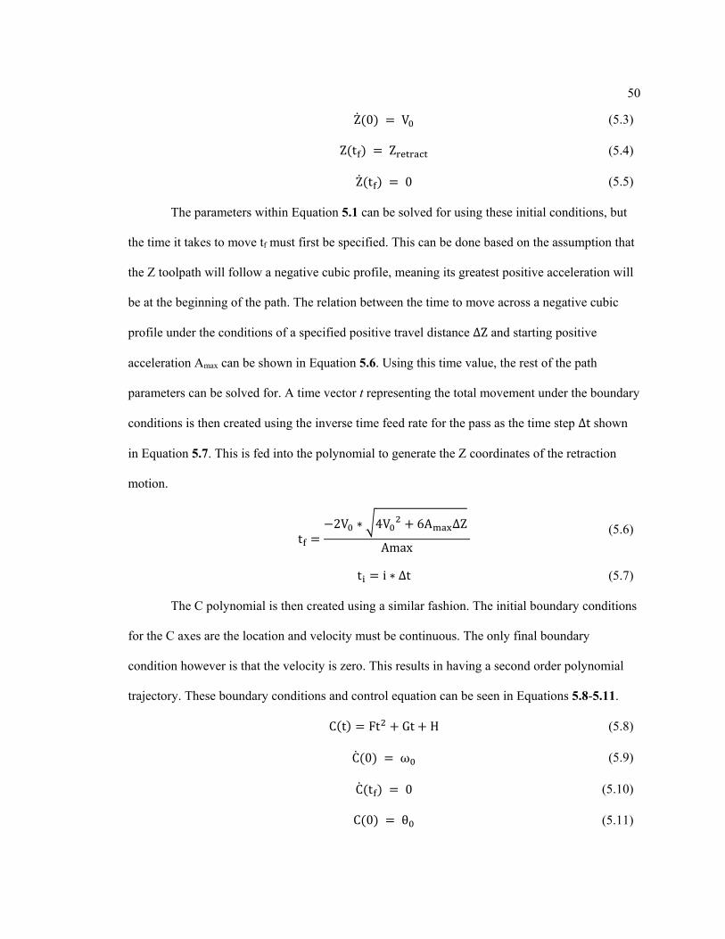
50
Z(0) = V0 (5.3)
Z(tf) = Zretract (5.4)
Z(tf) = 0 (5.5)
The parameters within Equation 5.1 can be solved for using these initial conditions, but
the time it takes to move tf must first be specified. This can be done based on the assumption that
the Z toolpath will follow a negative cubic profile, meaning its greatest positive acceleration will
be at the beginning of the path. The relation between the time to move across a negative cubic
profile under the conditions of a specified positive travel distance ∆Z and starting positive
acceleration Amax can be shown in Equation 5.6. Using this time value, the rest of the path
parameters can be solved for. A time vector t representing the total movement under the boundary
conditions is then created using the inverse time feed rate for the pass as the time step ∆t shown
in Equation 5.7. This is fed into the polynomial to generate the Z coordinates of the retraction
motion.
tf =−2V0 ∗ �4V02 + 6Amax∆Z
Amax
(5.6)
ti = i ∗ ∆t (5.7)
The C polynomial is then created using a similar fashion. The initial boundary conditions
for the C axes are the location and velocity must be continuous. The only final boundary
condition however is that the velocity is zero. This results in having a second order polynomial
trajectory. These boundary conditions and control equation can be seen in Equations 5.8-5.11.
C(t) = Ft2 + Gt + H (5.8)
C(0) = ω0 (5.9)
C(tf) = 0 (5.10)
C(0) = θ0 (5.11)

51
Based on the assumption the starting velocity is positive, this will produce a negative
parabolic profile, ending at the maxima. Using this assumption, the parameters in Equation 5.18
can then be solved for based on the time for move tf. This parameter is initially assumed to be the
same value as the Z movement took. The equation parameters can then be solved to produce the
C trajectory. Assuming the same time to move as in the Z path tf, the constant spindle
acceleration can be obtained using the initial speed ω0 shown in Equation 5.13, which is used to
check that no limits are violated in the profile. If the acceleration is above the maximum value
allowed, the C movement time is adjusted accordingly. The time vector is then generated and fed
into the C polynomial to generate the coordinates.
Cmax = −ω0
2𝑡𝑡𝑓𝑓 (5.12)
If this rotational ramp down period is longer than the Z movement period, the Z
coordinate is simply held at the retraction height after its movement while the spindle ramps
down. The X coordinate is held at the last value of the cutting toolpath across all these retraction
positions. The position, velocity, and acceleration of each axis for this retraction is depicted
below in Figure 5-2.

52
(a)
(b)
0 0.1 0.2 0.3 0.4 0.5 0.6 0.7
Time / s
0
0.05
0.1
X Po
sitio
n / m
m
Position
0 0.1 0.2 0.3 0.4 0.5 0.6 0.7
Time / s
-1
-0.5
0
X Ve
loci
ty /
mm
/s
Velocity
0 0.1 0.2 0.3 0.4 0.5 0.6 0.7
Time / s
0
200
400
600
X Ac
cele
ratio
n / m
m/s
2
Acceleration
0 0.1 0.2 0.3 0.4 0.5 0.6 0.7
Time / s
0
500
C P
ositi
on /
deg
Position
0 0.1 0.2 0.3 0.4 0.5 0.6 0.7
Time / s
0
100
200
C V
eloc
ity /
RPM
Velocity
0 0.1 0.2 0.3 0.4 0.5 0.6 0.7
Time / s
0
200
400
600
C A
ccel
erat
ion
/ rad
/s2
Acceleration

53
fcn_Retraction
[Retract] = fcn_Retraction(passes,maxSpeed,retractHeight)
This function outputs a cell array containing m elements, with a nx4 matrix in each
element containing the path information for the retraction. The arguments used and their relation
between the local variables and program variables can be seen below in Tables 5-3 and 5-4. The
full code can be seen in Appendix A-16.
The function begins by calculating the time needed according to the max Z acceleration
using the method presented above. This is then used to do a max velocity check to ensure no
(c)
Figure 5-2: Trajectory positions, velocities, and accelerations for the retraction path with the cutting path shown in blue and the retraction path shown in red. The graphs are split by (a) X axis (b) C axis (c) Z axis.
0 0.1 0.2 0.3 0.4 0.5 0.6 0.7
Time / s
0
2
4
Z Po
sitio
n / m
m
Position
0 0.1 0.2 0.3 0.4 0.5 0.6 0.7
Time / s
0
10
20
Z Ve
loci
ty /
mm
/s
Velocity
0 0.1 0.2 0.3 0.4 0.5 0.6 0.7
Time / s
-200
0
200
Z Ac
cele
ratio
n / m
m/s
2
Acceleration

54
speed limits are surpassed and adjusted accordingly. This time is then used with the C polynomial
to check maximum angular acceleration and spindle power and adjusted accordingly. Finally, a
for loop iterates through each pass and creates the time vector and finds the coordinates using the
polynomial projection equations. The matrices generated from each pass are stored in cell arrays
since the assumption cannot be made that they will be the same size.
Table 5-3: Table containing the information of the input arguments, output arguments, and any internal program variables accessed for fcn_Retraction
Input Arguments passes - Matrix containing all the cutter path information 3-D Matrix
3-Dimensional matrix that contains all the information for either the roughing or finishing passes. maxSpeed - Limit on Z velocity Scalar Limit on the maximum linear speed attained by the Z axis in retraction retractHeight - Z coordinate to retract to Scalar Represents the height that every retraction path will end at Output Arguments Retract - Contains all path information for retraction Cell Array
Cell array where each cell contains a matrix with the retraction path information for each pass of either the rouging or finishing passes Internal Variables Called maxVel - Maximum linear travel speed Scalar |4 m/min (default) Machine limit for linear travel speed maxAccel - Maximum linear travel acceleration Scalar |.05 g's (default) Machine limit for linear acceleration maxAngularAccel - Machine limit on spindle acceleration Scalar | 31 rad/s^2 (default) Machine limit for spindle acceleration maxPower - Spindle power limit Scalar | 1000 W (default) Used to check spindle power limit is not violated

55
5.2.2 Entry Path Generation
The purpose of the entry portion of a path is to allow the spindle to come up to constant
speed and then maintain constant speed to enter the cutting potion of a pass smoothly. Its
structure can be split into two sections accordingly. The path shape is determined by “expanding”
the driver spiral outwards following the constant X axis feed and angular spacing.
During the ramp up period, the dominating factor is for the spindle to ramp up smoothly,
which is controlled by another polynomial trajectory. Starting from a stopped position gives
greater flexibility in the conditions applied to the polynomial. The chosen initial conditions are
the position, velocity, and acceleration are all zero. The final conditions are the spindle speed is
equal to the beginning of the cutting path ωf and the acceleration is zero. This results in a fourth
momentOfInterita - Rotational moment of inertia of machine setup Scalar | .035879 kg*m^2 (default)
Solidworks calculated moment of inertia of the machining setup, used in conjunction with maxPower maxAccelMaragin - Optional scaling factor for maxAccel Scalar | .5 (default) Machine limit for linear travel speed
Table 5-4: Table showing the relations between the program’s structure arrays and the local variables within fcn_Retraction
MasterFlash Function Units
ROUGH/FINISH.toolPaths → passes [mm,rad,mm,seconds] SETUP.maxMoveSpeed → maxSpeed [mm/s]
SETUP.retractHeight → retractHeight [mm] ROUGH/FINISH.retract ← Retract {pass}[mm,rad,mm,seconds]
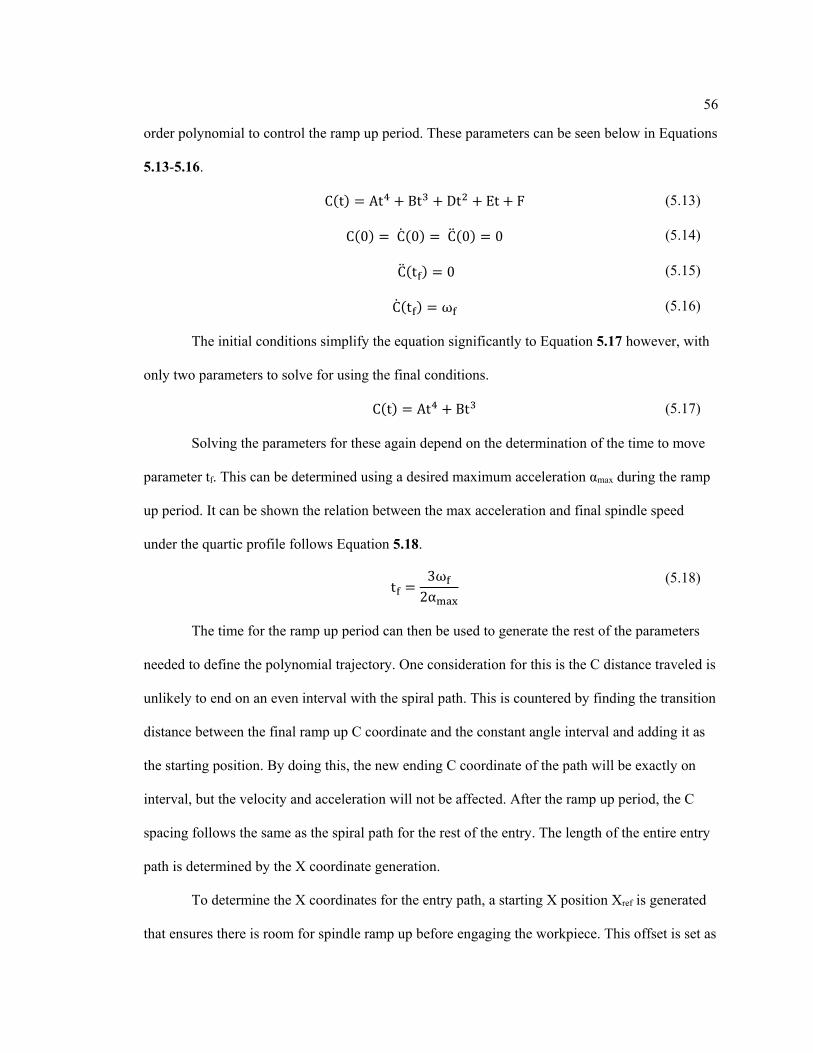
56
order polynomial to control the ramp up period. These parameters can be seen below in Equations
5.13-5.16.
C(t) = At4 + Bt3 + Dt2 + Et + F (5.13)
C(0) = C(0) = C(0) = 0 (5.14)
C(tf) = 0 (5.15)
C(tf) = ωf (5.16)
The initial conditions simplify the equation significantly to Equation 5.17 however, with
only two parameters to solve for using the final conditions.
C(t) = At4 + Bt3 (5.17)
Solving the parameters for these again depend on the determination of the time to move
parameter tf. This can be determined using a desired maximum acceleration αmax during the ramp
up period. It can be shown the relation between the max acceleration and final spindle speed
under the quartic profile follows Equation 5.18.
tf =3ωf
2αmax (5.18)
The time for the ramp up period can then be used to generate the rest of the parameters
needed to define the polynomial trajectory. One consideration for this is the C distance traveled is
unlikely to end on an even interval with the spiral path. This is countered by finding the transition
distance between the final ramp up C coordinate and the constant angle interval and adding it as
the starting position. By doing this, the new ending C coordinate of the path will be exactly on
interval, but the velocity and acceleration will not be affected. After the ramp up period, the C
spacing follows the same as the spiral path for the rest of the entry. The length of the entire entry
path is determined by the X coordinate generation.
To determine the X coordinates for the entry path, a starting X position Xref is generated
that ensures there is room for spindle ramp up before engaging the workpiece. This offset is set as

57
a whole number of rotations times the X axis feed rate to ensure cutting engagement will begin
when C is zero with the cutting path. Now knowing the number of rotations, the total C distance
rotated through can be calculated and used to generate the rest of the evenly spaced C coordinates
after the spindle ramp up period. Using the complete C coordinates, feed rate fr, and Xref, the X
positions can be calculated using Equation 5.19.
Xi = Xref − Ci ∗ fr (5.18)
The determination of the Z coordinates will differ depending on whether the entry pass is
for a roughing pass or finishing pass due to progressive step down of Z coordinates in the
roughing paths. Both begin by using the workpiece radius Rworkpiece and the complete entry path C
coordinates as the X and C inputs respectively to the surface function to generate the Z
coordinates shown in Equation 5.19. The workpiece radius is used as the x value to smoothly
transition the dynamics of entering the outer edge of the cutting portion while ensuring no
interference between the cutter and edge happen as the tool is fed inwards.
Z(X, C) = surfaceFunciton(Rworkpiece, Centry) (5.19)
These coordinates are then compensated for the cutter radius using the same method as
earlier used in the algorithm. For the finishing passes, each entry path is offset using the
respective Z cutting path offset calculated during the finish cutting calculations to create the
cutter locations. The roughing passes use a modified version of this. First the offset to the
finishing boundary is added to the Z coordinate of all the roughing entries. Then each pass is
compared to its roughing cut pass and the lowest Z coordinate in the cut path is set as the lower
boundary for the entry path. Any values below the boundary are set as the boundary value. This
correctly offsets the Z cutter locations without overcutting in the roughing passes. With the
completion of this step, the complete set of X, C, and Z cutter locations are generated for the
entry paths. An example of these entry paths can be seen below in Figure 5-3 for roughing and
Figure 5-4 for finishing.

58
(a)
0 0.5 1 1.5 2 2.5
Time / s
26
28
30
X Po
sitio
n / m
m
Position
0 0.5 1 1.5 2 2.5
Time / s
-2
-1
0
X Ve
loci
ty /
mm
/s
Velocity
0 0.5 1 1.5 2 2.5
Time / s
-2
-1
0
X Ac
cele
ratio
n / m
m/s
2
Acceleration
0 0.5 1 1.5 2 2.5
Time / s
0
500
1000
C P
ositi
on /
deg
Position
0 0.5 1 1.5 2 2.5
Time / s
0
100
200
C V
eloc
ity /
RPM
Velocity
0 0.5 1 1.5 2 2.5
Time / s
0
10
20
C A
ccel
erat
ion
/ rad
/s2
Acceleration

59
(b)
(c)
Figure 5-3: Trajectory positions, velocities, and accelerations for a roughing entry path with the cutting-portion shown in blue and the entry portion shown in green. The graphs are split by (a) X axis (b) C axis (c) Z axis.
0 0.5 1 1.5 2 2.5
Time / s
-0.4
-0.2
0Z
Posi
tion
/ mm
Position
0 0.5 1 1.5 2 2.5
Time / s
-5
0
5
Z Ve
loci
ty /
mm
/s
Velocity
0 0.5 1 1.5 2 2.5
Time / s
0
500
1000
Z Ac
cele
ratio
n / m
m/s
2
Acceleration

60
(a)
(b)
0 0.5 1 1.5 2 2.5 3
Time / s
26
28
X Po
sitio
n / m
m
Position
0 0.5 1 1.5 2 2.5 3
Time / s
-1
-0.5
0
X Ve
loci
ty /
mm
/s
Velocity
0 0.5 1 1.5 2 2.5 3
Time / s
-1
-0.5
0
X Ac
cele
ratio
n / m
m/s
2
Acceleration
0 0.5 1 1.5 2 2.5 3
Time / s
0
1000
2000
C P
ositi
on /
deg
Position
0 0.5 1 1.5 2 2.5 3
Time / s
0
100
200
C V
eloc
ity /
RPM
Velocity
0 0.5 1 1.5 2 2.5 3
Time / s
0
10
20
C A
ccel
erat
ion
/ rad
/s2
Acceleration

61
fcn_EntryPasses
[EntryPasses] = fcn_EntryPasses(toolPath,feedRate,cutterRadius, surfaceFcn,workpieceRadius)
This function outputs a cell array containing m elements, with a nx4 matrix in each
element containing the path information for the entry path. The arguments used and their relation
between the local variables and program variables can be seen below in Tables 5-5 and 5-6. The
full code can be seen in Appendix A-17.
Following the process outlined above, the total time for the ramp up portion of the entry
path is first calculated along with the other polynomial parameters. Additionally, the number of
(c)
Figure 5-4: Trajectory positions, velocities, and accelerations for a finishing entry path with the cutting portion shown in blue and the entry portion shown in green. The graphs are split by (a) X axis (b) C axis (c) Z axis.
0 0.5 1 1.5 2 2.5 3
Time / s
-0.5
0
Z Po
sitio
n / m
m
Position
0 0.5 1 1.5 2 2.5 3
Time / s
-5
0
5
Z Ve
loci
ty /
mm
/s
Velocity
0 0.5 1 1.5 2 2.5 3
Time / s
-100
0
100
Z Ac
cele
ratio
n / m
m/s
2
Acceleration

62
passes is calculated using the X offset. The function then enters a loop iterating through each
pass. The ramp up period C coordinates are created and offset for the transition, followed by
adding the constant spacing C coordinates. The X and Z coordinates are then calculated
accordingly, but the Z coordinates are not compensated or offset yet. These cutter locations are
output in cell arrays again for data modularity if the paths end up not being the same lengths. The
cutter compensation is performed in the algorithm to match whichever compensation was used
for the cutting path. After this is done, the cutting offsets are added through fcn_EntryOffset, full
code in A-18, in the algorithm using the offset information generated during fcn_MachiningSetup.
Table 5-5: Table containing the information of the input arguments, output arguments, and any internal program variables accessed for fcn_EntryPasses
Input Arguments toolPath - Matrix containing all the cutter path information 3-D Matrix
3-Dimensional matrix that contains all the information for either the roughing or finishing passes. feedRate - X axis feed rate Scalar Value for the constant X axis feed rate cutterRadius - Diamond cutter radius Scalar Size of the diamond turning tool cutter radius, used in clearance calcs surfaceFcn – Handle calling surface function Handle MATLAB handle for calling surface function file workpieceRadius – Radius of workpiece Scalar Size of the radius of the workpiece Output Arguments EntryPasses - Cutter locations of entry passes Cell Array
Cell array where each cell contains a matrix with the entry path information for each pass of either the rouging or finishing passes

63
5.3 Final Cutting Pass Preparation
At this point in the algorithm, all the cutter locations have been calculated are contained
in the three classes entries, toolPaths, and retract. These variables contain all the relevant cutter
locations for post processing into G-code, but there is some final processing to this data to make it
work.
The first step is to update the units associated with the C coordinates. Until this point in
the program, the C data has been stored and used exclusively in radians, however the machine
units are in degrees. The function fcn_ConvertC, full code in Appendix A-19, takes in all three
classes and outputs these converted coordinates.
Internal Variables Called accelScale - Acceleration scaling factor Scalar | 0.6 (default) Scaling factor to control spindle acceleration during ramp up maxAngularAccel - Machine limit on spindle acceleration Scalar | 31 rad/s^2 (default) Machine limit for spindle acceleration entryLength - Clearance offset Scalar | 2.5 mm (default) Offset added in X axis to allow spindle ramp up
Table 5-6: Table showing the relations between the program’s structure arrays and the local variables within fcn_EntryPasses
MasterFlash Function Units
ROUGH/FINISH.toolPaths → toolPath [mm,rad,mm,seconds] ROUGH/FINISH.feedRate → feedRate [mm/rev]
SETUP.cutterRadius → cutterRadius [mm] surfaceFcn → surfaceFcn [handle]
SETUP.workpieceRadius → workpieceRadius [mm] ROUGH/FINISH.entries ← EntryPasses {pass}[mm,rad,mm,seconds]
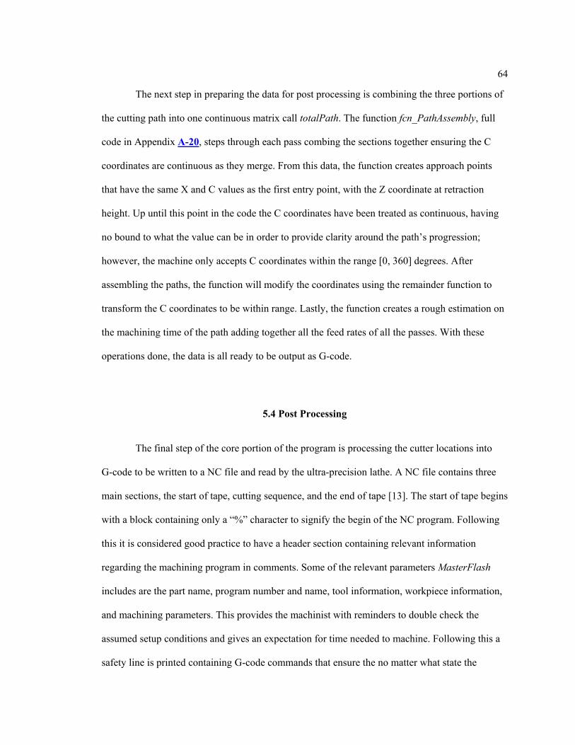
64
The next step in preparing the data for post processing is combining the three portions of
the cutting path into one continuous matrix call totalPath. The function fcn_PathAssembly, full
code in Appendix A-20, steps through each pass combing the sections together ensuring the C
coordinates are continuous as they merge. From this data, the function creates approach points
that have the same X and C values as the first entry point, with the Z coordinate at retraction
height. Up until this point in the code the C coordinates have been treated as continuous, having
no bound to what the value can be in order to provide clarity around the path’s progression;
however, the machine only accepts C coordinates within the range [0, 360] degrees. After
assembling the paths, the function will modify the coordinates using the remainder function to
transform the C coordinates to be within range. Lastly, the function creates a rough estimation on
the machining time of the path adding together all the feed rates of all the passes. With these
operations done, the data is all ready to be output as G-code.
5.4 Post Processing
The final step of the core portion of the program is processing the cutter locations into
G-code to be written to a NC file and read by the ultra-precision lathe. A NC file contains three
main sections, the start of tape, cutting sequence, and the end of tape [13]. The start of tape begins
with a block containing only a “%” character to signify the begin of the NC program. Following
this it is considered good practice to have a header section containing relevant information
regarding the machining program in comments. Some of the relevant parameters MasterFlash
includes are the part name, program number and name, tool information, workpiece information,
and machining parameters. This provides the machinist with reminders to double check the
assumed setup conditions and gives an expectation for time needed to machine. Following this a
safety line is printed containing G-code commands that ensure the no matter what state the

65
machine was left in; the program will be able to run without any problems. MasterFlash’s safety
line sets the machine to absolute coordinates, sets the plane to XZ, cancels any on machine radius
compensation, sets the units to metric, sets G54 as the work coordinate, sets the machine to radius
mode, and sets the linear feed rates to feed per minute.
Following the safety line, the cutting sequence can begin. It initializes by setting the
machine to M78 C-axis mode, giving control over the C axis. The machine then goes to the home
position, which is zero for the X and C coordinates, and the retract height for the Z coordinate.
This completes the initialization for cutting. From here a for loop steps through every pass
completing the same sequence for roughing and then finishing. The machine is set to G94 feed
per minute mode to travel at a specified feed rate using G01 linear move first to the approach
position and then to the initial entry position. Here the machine is set to G93 inverse time and
specifying the modal feed rate. Each position is then stepped through moving with G01 for the
path and printed based on a rule set. This is needed because there can be millions of positions to
be printed, so printing rules are enforced in effort to reduce the file size. The first rule is G01 is
modal, so only the coordinates that change from point to point need printed. As the X and C
coordinates are set at a constant feed rate, they will need printed on every line. However, the Z
coordinate only needs printed if it changes from the previous position. In addition to this, the
program checks if the number being printed for the C coordinates is capable of being printed as
an integer or smaller decimal without losing any accuracy. This can save the space that would be
used to print the 5 decimal points of precision in the C coordinate. The X and Z coordinates are
printed to six decimals of precision. An example couple blocks of code implementing these rules
can be seen below in Figure 5-5.

66
After all the pass printing loops complete, the end of tape sequence is printed. First the
machine is set back to back to G94 feed per minute travel mode and the Z is backed off further
from the workpiece to provide easier access to the workpiece. To leave the machine in a
predictable state the end of tape also sets the machine to absolute coordinates, ensures any cutter
comp has been cancelled, sets the machine to metric, and sets the machine to radius mode. These
are repetitive and should not be changed during the process, but in case anything in the program
is changed later, the machine will always be left in a predictable state. The program then
concludes with a “%” character to signify the end of the program.
fcn_NCFileWrite
[] = fcn_NCFileWrite(POST,SETUP,ROUGH,FINISH)
This function creates a NC file and writes all the relevant G-code to machine the desired
surface. The arguments used and their relation between the local variables and program variables
can be seen below in Tables 5-7 and 5-8. The full code can be seen in Appendix A-21.
The writing of the NC file is the most time-consuming process during the completion of
the program. Due to this, the file begins by displaying the expected surface roughness, which can
be estimated using the height of the scallop left behind h in Equation 5.20 [24], [38], the total
Figure 5-5: Example excerpt of outputted G-code for G01 command from a roughing pass.

67
number of passes, and the estimated machine time to the user to give the user a chance to opt out
of the program before investing the time to continue if something does not look right. It is
important to note Equation 5.20 is a prediction of the ideal surface roughness; it does not account
for material effects, vibrations, movement error, or edge condition of the cutter.
ℎ =
𝑓𝑓𝑟𝑟2
8 𝑅𝑅𝑐𝑐𝑐𝑐𝑐𝑐𝑐𝑐𝑐𝑐𝑟𝑟𝜔𝜔2 (5.20)
If the user chooses to continue, the program tries to create a NC file according to the
name provided on the input script. If a file with the same name already exists in the job folder
from a previous run, the program will prompt the user to enter a new name or overwrite the
previous file. Finally, the program will print the opening section, step through each roughing
pass, step through each finishing pass, print the closing section, and then close the file.
Table 5-7: Table containing the information of the input arguments, output arguments, and any internal program variables accessed for fcn_NCFileWrite
Input Arguments POST - Matrix containing all the cutter path information Structure Array
3-Dimensional matrix that contains all the information for either the roughing or finishing passes. SETUP – X axis feed rate Structure Array Value for the constant X axis feed rate ROUGH – Diamond cutter radius Structure Array Size of the diamond turning tool cutter radius, used in clearance calcs FINISH – Handle calling surface function Structure Array MATLAB handle for calling surface function file Internal Variables Called coolantOn – Desired coolant G-code String | M07 (default) G-code for the desired coolant on command. *Used as a placeholder for not, not implemented*

68
coolantOff - Machine limit on spindle acceleration String | M09 (default) G-code for the desired coolant off command. Use to toggle between flood and mist*Used as a placeholder for not, not implemented* gsafety – Safety line implemented at beginning of program String Safety block implemented at the beginning of a NC program to make sure no matter what state the machine was left at, the program will run correctly. gend – Secondar Safety block used at the end of the program String | 2.5 mm (default) Block added at the end of a program to ensure the machine is always left in a predictable state.
Table 5-8: Table showing the relations between the program’s structure arrays and the local variables within fcn_NCFileWrite
MasterFlash Function Units
POST → POST [] SETUP → SETUP []
ROUGH → ROUGH [] FINISH → FINISH []

Chapter 6
Optional Program Checks
Outside of the core section of the program in MasterFlash, there are several optional
sections that can be implemented that are not necessary to producing the G-code but can be very
helpful to have a successfully turned part. These optional checks can be divided into checks
relating to the choice of diamond turning tool for the surface and checks to make sure the path
generation came out as expected.
6.1 Diamond Turning Tool Optimization
With the surface complexity that is possible when using freeform surfaces, Fang et al
note it is wise to check the diamond turning tool parameters to make sure the tool used will not
cause interference or profile errors with the surface [24]. The program automatically offsets for
the cutter radius compensation, but it does not automatically check for interference from
parameters such as the included angle ϴIA, clearance angle ϴCA, or that the tool radius Rcutter is too
large. These parameters are visualized on the cutter below in Figure 6-1. MasterFlash includes
these optional checks through the fcn_ToolOptimization, full code shown in Appendix A-22,
which is used to call the individual functions checking each parameter. This function will call
each parameter check function using the path’s control points as a basis, print the minimum or
max value for each check, and compare it to the chosen tool’s parameters. If any geometry
constraints are violated, the function will produce a MATLAB warning message to the user in the
command window to alert the programmer.

70
6.1.1 Cutter Radius Check
The cutter radius is offset in space to avoid cutting interference, but there could exist a
condition where the cutter radius is too large for the radius of curvature of the surface in a
concave section, leading to an undercut. For analysis of cutter radius optimization, the surface is
first broken down into sectional curves shown in Figure 6-2 by using a variety of constant angle
sections, producing the curve profiles that would be parallel with the cutting plane of the tool.
Figure 6-1: Top and side views of the diamond cutter insert with the included angle, cutter radius, and clearance angle identified
Included Angle
Clearance Angle
CutterRadius

71
The derivative and double derivative are then taken at each point along the sectional curve.
Concave sections are identified by where the derivative switches from negative to positive as the
X value increases. The nearest inflections to these concave points are then identified, identified
where the double derivative changes signs. The distance to the closest inflection to each concave
point is then calculated and used to offset the concave point in both directions along X to produce
points e1 and e2. These two points and the concave point are then used to fit a circle using the
double bisection method shown in Figure 6-3. For double bisection, first the three points are
turned into a set of two intersecting lines. From these two lines perpendicular bisectors are
extended until they intersect. The intersection of the bisectors represents the fitted circle’s center.
The distance between this center and one of the fitted points represents the radius of the circle.
Figure 6-2: Sectional curve breakdown to check the cutter radius [39]
Sectional Curve
Inflection PointInflection Point
e_1
e_2
Concave Point (a)
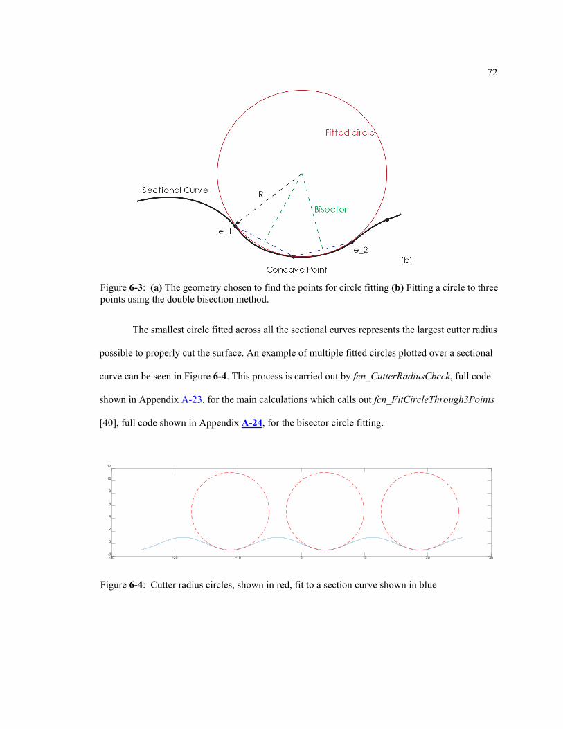
72
The smallest circle fitted across all the sectional curves represents the largest cutter radius
possible to properly cut the surface. An example of multiple fitted circles plotted over a sectional
curve can be seen in Figure 6-4. This process is carried out by fcn_CutterRadiusCheck, full code
shown in Appendix A-23, for the main calculations which calls out fcn_FitCircleThrough3Points
[40], full code shown in Appendix A-24, for the bisector circle fitting.
Figure 6-3: (a) The geometry chosen to find the points for circle fitting (b) Fitting a circle to three points using the double bisection method.
Figure 6-4: Cutter radius circles, shown in red, fit to a section curve shown in blue
-30 -20 -10 0 10 20 30-2
0
2
4
6
8
10
12

73
6.1.2 Included Angle Check
The included angle is checked to make sure only the curved portion of the cutter meets
the finished workpiece. If the straight edges beyond the curve portion are in contact, the surface is
steeper than the cutter edge and therefor will get overcut shown in Figure 6-5. The included angle
check operates similarly to the sectional curves method to check geometry. The constant angle
curve is used, but in this case only the first derivative of the curve with respect to the X
coordinate is needed. The derivative is used in conjunction with the inverse tangent function to
determine the slope of the surface at each point in degrees. To ensure the cutter only contacts
within the curved portion of the cutting edge to avoid overcutting, the included angle needs to
follow the relation shown below in Equation 6.1. This is checked using fcn_IncludedAngleCheck,
full code shown in Appendix A-25.
𝜃𝜃𝐼𝐼𝐼𝐼 ≤ 2 �𝜋𝜋2− |𝑁𝑁tan (𝑠𝑠𝑁𝑁𝑓𝑓𝑠𝑠𝑠𝑠)|� (6.1)
Figure 6-5: Included angle related interference is highlighted in red

74
6.1.3 Clearance Angle Check
The final diamond turning tool parameter to check is the clearance angle. The intent of
this check is to make sure the tool’s flank face does not interfere with the cut surface. For this
check, the parametric path is simplified to a two-dimensional curve using the Z and C
coordinates. The slopes of this parametric curve are calculated at every control point and
converted to degrees using the inverse tangent function. To avoid interference, the clearance
angle needs be greater than the most positive slope found in the control points. This is carried out
by the function fcn_ClearanceAngleCheck, full code shown in Appendix A-26.
6.2 Path Generation Checks
After the creation of the NC file, it is convenient to double check that the path generation
completed correctly before running the program on the machine. MasterFlash implements these
checks by running fcn_PostChecks, full code shown in Appendix A-27, after the completion of
the post processing. Key areas of interest to make sure they transitioned smoothly are the entry
and exit of the cutting paths. The post checks function presents figures showing these transitions
for the X, C, and Z coordinates for position, velocity, and acceleration for a roughing and a
finishing pass. The figures follow the format of Figures 5.2-5.4, which allows the user to confirm
these transitions follow the expected behavior. Finally, a three-dimensional graph is produced
with the final finishing pass to confirm the surfaces matches expectations.

Chapter 7
Program Verification
With the G-code successfully generated it was validated by turning four test workpieces
on the Moore Nanotechnology UPL 350. The tool centering procedure, material selection,
algorithm selection, and machining parameters will be covered.
7.1 Centering the Diamond Turning Tool
The first step in program verification was mounting the and centering the diamond
turning tool. This is starts by aligning the rake face of the diamond turning tool to be exact with
the center of the workpiece. This is done by taking repeated facing passes and examining the
workpiece center under high magnification for the characteristics shown in Figure 7-1. If there
remains a cone shape at the center of the workpiece, the tool needs to be adjusted downwards. If
there remains a cylindrical shape, the tool needs to be adjusted upwards[40]. The tool holding
assembly on the UPL 350 allows for a rough and very fine adjustment to achieve these actions
accurately.
Figure 7-1: Depiction for centering the Z height of a diamond tool (a) too low and (b) too high [39].

76
With the Z height set, the X is then centered using the work coordinate offsets following
the same iterative facing procedure. After each pass the workpiece is removed and examined at
high magnification. If the X coordinate is being undercut, there will be a distinct plateau shape at
the center that was not machined. If the X coordinate is overcut, there will be a section of
overcutting characterized by a “W” shaped grove. Examples of these conditions can be seen in
Figure 7-2. The X offset for the work coordinate gets changed accordingly to make the tool
centered on the workpiece.
7.2 Stock Material and Tool Selection
Each workpiece used was chosen to be oxygen free copper (OFC). The substrate has
good machinability and will not wear the turning tool out quickly. With the machining times
being proportional to the radius of the workpieces, 7/16-inch stock was chosen to reduce
Figure 7-2: Depiction for centering the X height of a diamond tool (a) undercut center cylinder and (b) overcut characteristic “W” shape.
Z
Z
Undercut
Overcut
(a)
(b)
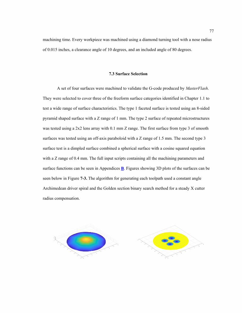
77
machining time. Every workpiece was machined using a diamond turning tool with a nose radius
of 0.015 inches, a clearance angle of 10 degrees, and an included angle of 80 degrees.
7.3 Surface Selection
A set of four surfaces were machined to validate the G-code produced by MasterFlash.
They were selected to cover three of the freeform surface categories identified in Chapter 1.1 to
test a wide range of surface characteristics. The type 1 faceted surface is tested using an 8-sided
pyramid shaped surface with a Z range of 1 mm. The type 2 surface of repeated microstructures
was tested using a 2x2 lens array with 0.1 mm Z range. The first surface from type 3 of smooth
surfaces was tested using an off-axis paraboloid with a Z range of 1.5 mm. The second type 3
surface test is a dimpled surface combined a spherical surface with a cosine squared equation
with a Z range of 0.4 mm. The full input scripts containing all the machining parameters and
surface functions can be seen in Appendices B. Figures showing 3D plots of the surfaces can be
seen below in Figure 7-3. The algorithm for generating each toolpath used a constant angle
Archimedean driver spiral and the Golden section binary search method for a steady X cutter
radius compensation.
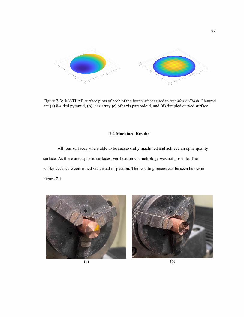
78
7.4 Machined Results
All four surfaces where able to be successfully machined and achieve an optic quality
surface. As these are aspheric surfaces, verification via metrology was not possible. The
workpieces were confirmed via visual inspection. The resulting pieces can be seen below in
Figure 7-4.
Figure 7-3: MATLAB surface plots of each of the four surfaces used to test MasterFlash. Pictured are (a) 8-sided pyramid, (b) lens array (c) off axis paraboloid, and (d) dimpled curved surface.
(a)
(b)

79
(c)
(d)
(e)
(f)
(g) (h)
Figure 7-4: Pictures showing the final machined surfaces. (a)&(b) 8-sided pyramid (c)&(d) 2x2 micro lens array (e)&(f) dimpled surface
Chapter 8
Conclusion
A CAM program for single point diamond turning was successfully developed with a
flexible framework and verified by turning four freeform optical surfaces successfully. The four
chosen surfaces contained a diverse set of characteristics that were all able to be handled by the
program effectively. Beyond the ability to be able to machine these beautifully complex freeform
optics using today’s current methods, the most exciting aspect of MasterFlash is the value the
program creates through the potential in using its framework for creating further research within
diamond turning and freeform optics. Its intent was to create a platform that is able to be
expanded upon and improved through the future.
Future Work
With the modular framework for MasterFlash implemented, there are many potential
areas of future work for expanding the program. The inclusion of negative rake angle tools, gang
tooling, or non-symmetric cutter geometry would further expand the possible materials and
geometries that are able to be machined respectively. The inclusion of a tool and machine library
would help improve the ease and simplicity of the input script. Further avenues of improvement
include creating a GUI for the input for increased understanding with user interaction. If this
route were to be taken, it should be considered switching to program to using Python as the
coding language for the utility of Python’s libraries for CAD programs and graphical display. The
biggest limitation of the current program is the lack of metrology resources available to fully
examine the optical surfaces created to fine tune parameters within the program. This should be

81
evaluated through expanded tests and measurement and verification in the future stages of the
program.
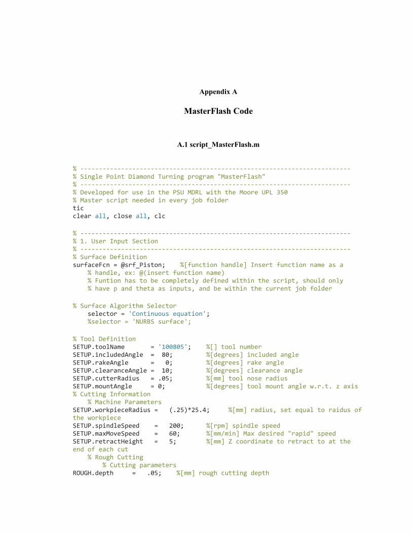
Appendix A
MasterFlash Code
A.1 script_MasterFlash.m
% ------------------------------------------------------------------------- % Single Point Diamond Turning program "MasterFlash" % ------------------------------------------------------------------------- % Developed for use in the PSU MDRL with the Moore UPL 350 % Master script needed in every job folder tic clear all, close all, clc % ------------------------------------------------------------------------- % 1. User Input Section % ------------------------------------------------------------------------- % Surface Definition surfaceFcn = @srf_Piston; %[function handle] Insert function name as a % handle, ex: @(insert function name) % Funtion has to be completely defined within the script, should only % have p and theta as inputs, and be within the current job folder % Surface Algorithm Selector selector = 'Continuous equation'; %selector = 'NURBS surface'; % Tool Definition SETUP.toolName = '100805'; %[] tool number SETUP.includedAngle = 80; %[degrees] included angle SETUP.rakeAngle = 0; %[degrees] rake angle SETUP.clearanceAngle = 10; %[degrees] clearance angle SETUP.cutterRadius = .05; %[mm] tool nose radius SETUP.mountAngle = 0; %[degrees] tool mount angle w.r.t. z axis % Cutting Information % Machine Parameters SETUP.workpieceRadius = (.25)*25.4; %[mm] radius, set equal to raidus of the workpiece SETUP.spindleSpeed = 200; %[rpm] spindle speed SETUP.maxMoveSpeed = 60; %[mm/min] Max desired "rapid" speed SETUP.retractHeight = 5; %[mm] Z coordinate to retract to at the end of each cut % Rough Cutting % Cutting parameters ROUGH.depth = .05; %[mm] rough cutting depth
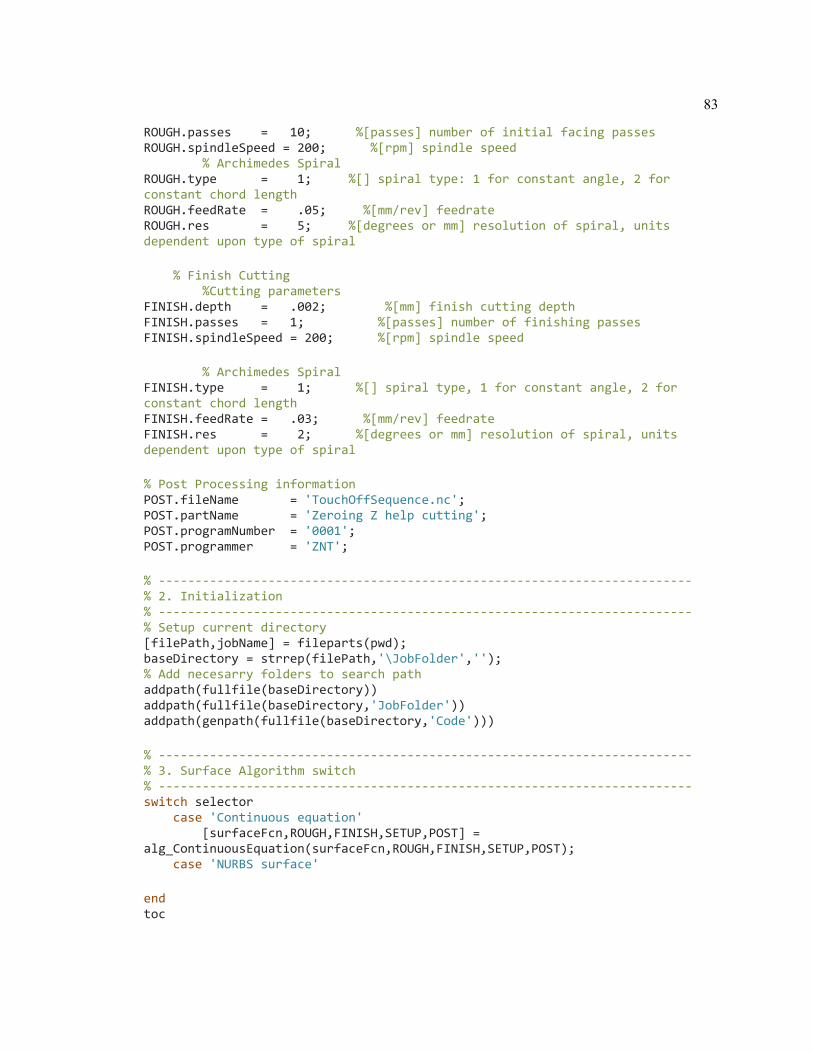
83
ROUGH.passes = 10; %[passes] number of initial facing passes ROUGH.spindleSpeed = 200; %[rpm] spindle speed % Archimedes Spiral ROUGH.type = 1; %[] spiral type: 1 for constant angle, 2 for constant chord length ROUGH.feedRate = .05; %[mm/rev] feedrate ROUGH.res = 5; %[degrees or mm] resolution of spiral, units dependent upon type of spiral % Finish Cutting %Cutting parameters FINISH.depth = .002; %[mm] finish cutting depth FINISH.passes = 1; %[passes] number of finishing passes FINISH.spindleSpeed = 200; %[rpm] spindle speed % Archimedes Spiral FINISH.type = 1; %[] spiral type, 1 for constant angle, 2 for constant chord length FINISH.feedRate = .03; %[mm/rev] feedrate FINISH.res = 2; %[degrees or mm] resolution of spiral, units dependent upon type of spiral % Post Processing information POST.fileName = 'TouchOffSequence.nc'; POST.partName = 'Zeroing Z help cutting'; POST.programNumber = '0001'; POST.programmer = 'ZNT'; % ------------------------------------------------------------------------- % 2. Initialization % ------------------------------------------------------------------------- % Setup current directory [filePath,jobName] = fileparts(pwd); baseDirectory = strrep(filePath,'\JobFolder',''); % Add necesarry folders to search path addpath(fullfile(baseDirectory)) addpath(fullfile(baseDirectory,'JobFolder')) addpath(genpath(fullfile(baseDirectory,'Code'))) % ------------------------------------------------------------------------- % 3. Surface Algorithm switch % ------------------------------------------------------------------------- switch selector case 'Continuous equation' [surfaceFcn,ROUGH,FINISH,SETUP,POST] = alg_ContinuousEquation(surfaceFcn,ROUGH,FINISH,SETUP,POST); case 'NURBS surface' end toc

84
A.2 var_internal.m
function varargout = var_internal(identifier) % Programmer: Zachary Timothy % Last Updated: 10/07/2020 % Future Updates: % % Creates an easily modifiable set of internal variables used within the % program for fine tuning the path generation. For functions with relevant % variables, this will be called at their beginning to recieve the current % values % % Inputs: % identifier[string] - String input identifying which function is % calling for variables % % Outputs: % varargout[varies] - Variable output argument where each cell is the % respective value for the appropriate function's variables %% Common Machine Limit Variables maxAngularAccel = 31; %[rad/s^2] maxLinearSpeed = 4000/60; %[mm/s] maxLinearAccel = 0.05*9.81e3; %[mm/s^2] %% Variable assignment switch identifier %-------------------------------------------------------------------------- % 2_PathGeneration %-------------------------------------------------------------------------- % ExitInterpCA case 'ExitInterpCA' % extra = The number of additional points at center to append to prevent % move blending from retracting early varargout{1} = 5; %[points] %-------------------------------------------------------------------------- % 4_ToolOptimization %-------------------------------------------------------------------------- % ClearanceAngleCheck case 'ClearanceAngleCheck' % delta = Angular step resolution used for calculating the derivative of % the surface w.r.t. the change in angle varargout{1} = .0000001; %[rad] % CutterRadiusCheck case 'CutterRadiusCheck' % sections = number of cross sections to check for cutterRadius varargout{1} = 3; %[sections] % curveRes = linear resolution along the curve to check for fitting a % cirlce to check the radius

85
varargout{2} = 1e-5; %[mm] % IncludedAngleCheck case 'IncludedAngleCheck' % delta = linear step resolution to check along the path for finding % derivative of surface for included angle varargout{1} = .0000001; %[mm] %-------------------------------------------------------------------------- % 5_PostProcessing %-------------------------------------------------------------------------- % EntryPasses case 'EntryPasses' % accelScale = Safety factor to be applied for max planned spindle % acceleration for ramp up at entry varargout{1} = 0.6; %[scale] % maxAngularAccel = max machine angular acceleration for the air % spindle varargout{2} = maxAngularAccel; %[rad/s^2] % entryLength = distance to "cut air" before engaging with the stock varargout{3} = 2.5; %[mm] % --------------- Outdated -------------------------------- % maxSpeed = Max linear feedrate for the machine % % % varargout{4} = maxLinearSpeed; %[mm/s] % maxAcel = Max linear acceleration by machine % % % varargout{5} = maxLinearAccel; %[mm/s^2] % ---------------------------------------------------------- % InverseTimeCalcs case 'InverseTimeCalcs' % maxSpeed = Max linear feedrate for the machine varargout{1} = maxLinearSpeed; %[mm/s] % maxAcel = Max linear acceleration by machine varargout{2} = maxLinearAccel; %[mm/s^2] % maxSpeedScale = scaling factor to apply to machine max linear % movement speed varargout{3} = .5; %[] % NCFileWrite case 'NCFileWrite' % coolantOn = Gcode for turning on machine's coolant varargout{1} = 'M07'; % coolantOff = Gcode for turning off machine's coolant varargout{2} = 'M09'; % gsafety = line of Gcode to be printed at beginning of the program to % ensure everything is in order varargout{3} = 'G90 G18 G40 G71 G54 G63 G94 (Absolute, lathe, cancel radius comp, metric, work coordinate, radius, feed/min)\r\n'; % gend = line of Gcode to be printed at the end of the tape varargout{4} = 'G90 G40 G71 G63 (Absolute, cancel radius comp, metric, radius) \r\n M02\r\n%%\r\n';

86
% Retraction case 'Retraction' % maxVel = Max linear feedrate for the machine varargout{1} = maxLinearSpeed; %[mm/s] % maxAccel = Max linear acceleration for the machine varargout{2} = maxLinearAccel; %[mm/s^2] % maxAngularAccel = max machine angular acceleration for the air % spindle varargout{3} = maxAngularAccel; %[rad/s^2] % maxPower = Max desired power output from the spindle for precision varargout{4} = 1000; %[Watts] % momentOfInertia = Calculated average moment of inertia for machining, % calculated using Solidworks model with 6"x2" steel mount attached % with a 2" diameter workpiece. Used for power checks. varargout{5} = .035879; %[kg*m^2] % maxAccelMaragin = scaling factor to be applied to the acceleration varargout{6} = 0.5; %[scale] end end

A.3 fcn_ArchimedesSprial.m
function [X_Theta] = fcn_ArchimedesSpiral(type,fr,res,r) % Programmer: Zachary Timothy % Last Updated: 06/24/2020 % Future Updates: Re-examine constant arc length? % % Generates an Archimedes spiral over workpiece radius r using feed per % revolution fr % % Inputs: % type[] - switch for variation of spiral % Set type = 1 for a constant angular spiral, Res given in [degrees] % Set type = 2 for a constant arc length spiral, Res given in [mm] % fr[mm/rev] - feed rate % res[degrees or mm] - resolution of unit based on type % r[mm] - radius of workpiece % % Outputs: % Matrix X_Theta = [X,Theta] which consists of: % X[mm] - radial(X) values % Theta[radians] - angle(C) values %% Input Error Check % Type check switch type case 1 % Constant Angle % do nothing case 2 % Constant Arc Length % do nothing otherwise % Invalid type input, throw an error error('Invalid Type input, Use Type=1 for constant angle or Type=2 for constant chord length') end % Feed rate check if fr<=0 error('Invalid feed rate, must be greater than 0') end % Resolution check if res<=0 error('Invalid resoluiton, must be greater than 0') end % Radius check if r<=0 error('Invalid workpiece radius, must be greater than 0')

88
end %% Number of Points Calculation % Used to come up with length of preallocated vectors for speed % Total turns needed: nt nt = r / fr; %[turns] % Convert fr fr = fr / (2*pi); %[mm/rad] switch type case 1 % Constant Angle % Number of machining points: Np np = ceil(nt*360/res); %[points] % Initialize Theta Theta = zeros(np,1); %[radians] case 2 % Constant Arc Length % Create variable a to be used in length formula a = fr; %[mm/rad] % Find total angle rotated through with spiral u = nt*2*pi; %[rad] % Find total length of the spiral length = a/2*(u*sqrt(1+u^2)+log(u+sqrt(1+u^2))); %[mm] % Find number of points needed for the spiral np = floor(length/res); %[points] % Initialize Theta and P Theta = zeros(np,1); %[radians] P = zeros(np,1); %[mm] end %% Main calcs % Calculate the values for Theta and P switch type case 1 % Constant Angle % Convert res to radians res = deg2rad(res); %[radians] % For loop that generates the theta values needed for i = 2:np Theta(i) = Theta(i-1) + res; %[radians] end % Generate respective p values P = r - fr*Theta; %[mm] case 2 % Constant Arc % Initialize first point P(1) = r; %[mm] % Numerically generate points until negative P value is reached for i = 2:np % Find angle travelled over the chord distance deltaTheta = res / P(i-1); %[radians] % Update new angle using deltaTheta Theta(i) = Theta(i-1) + deltaTheta; %[radians] % Update new radius using deltaTheta P(i) = P(i-1) - fr * (deltaTheta); %[mm] end end

89
% Check P doesn't go negative and ends on 0 % Create zero check variable check = P(np); %[mm] % If loop comparing check to 0 if check <= 0 % If current last entry is below or equal to zero, change last radius to 0 P(np) = 0; %[mm] else switch type case 1 % Constant Angle % If current last entry is above zero, add one more element to % to radius with value of zero P(np+1) = 0; %[mm] % Add another element to Theta following the same spacing Theta(np+1) = Theta(np) + res; %[radians] case 2 % Constant Length % If current last entry is above zero, add one more element to % to radius with value of zero P(np+1) = 0; %[mm] % Add another element to Theta following the same spacing Theta(np+1) = Theta(np) + res / P(np); %[radians] end end % Create the output matrix X_Theta = [P,Theta]; end

A.4 srf_Zernike
function Z = fcn_Zernike(p,theta) % Programmer: Zachary Timothy % Last Updated: 05/28/2020 % Function that solves a zernike polynomial using the ANSI standard number % Takes vectors of p and theta and returns the z value based on a vector of ANSI standard Zernike coeffecients. % Current equation goes from 0 to 35. Note that the indices of the vector will be one off by one % Ensure the ANSIorder.m function is also in the folder for this to work % Coeffecients coeff = zeros(36,1); % Define desired coeffecients here by filling in the coeff vector coeff(1) = 1; coeff(17) = 0; coeff(9) = 0; p_max = 25.4; % Initialize Variables R = 0; Z = 0; z = 0; %Normalization of p p_norm = p/p_max; % ANSI Order Calc order = size(coeff)-1; for index = 0 : order % Begin Loop A: Order if coeff(index+1) == 0 % Check if coeffecient is nonzero % Do nothing else % Get the m and n for each order [m,n] = fcn_ANSIorder(index); %Calculation of R for s = 0 : ((n-abs(m))/2) % Begin Loop AB: R calc num = (-1)^s*factorial(n-s); den = factorial(s)*factorial(0.5*(n+abs(m))-s)*factorial(0.5*(n-abs(m))-s); R = R + num/den .* p_norm.^(n-2.*s); end % End Loop AB
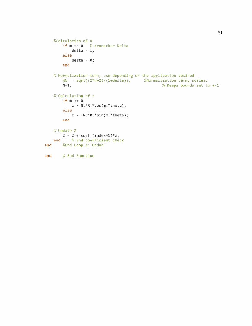
91
%Calculation of N if m == 0 % Kronecker Delta delta = 1; else delta = 0; end % Normalization term, use depending on the application desired %N = sqrt((2*n+2)/(1+delta)); %Normalization term, scales. N=1; % Keeps bounds set to +-1 % Calculation of z if m >= 0 z = N.*R.*cos(m.*theta); else z = -N.*R.*sin(m.*theta); end % Update Z Z = Z + coeff(index+1)*z; end % End coefficient check end %End Loop A: Order end % End Function

A.5 fcn_ANSIorder
function [m,n] = fcn_ANSIorder(order) % Function that determines the m and n values for a Zernike polynomial % based off the ANSI coeffecient switch order case 0 m = 0; n = 0; case 1 m = -1; n = 1; case 2 m = 1; n = 1; case 3 m = -2; n = 2; case 4 m = 0; n = 2; case 5 m = 2; n = 2; case 6 m = -3; n = 3; case 7 m = -1; n = 3; case 8 m = 1; n = 3; case 9 m = 3; n = 3; case 10 m = -4; n = 4; case 11 m = -2; n = 4; case 12 m = 0; n = 4; case 13 m = 2; n = 4;

93
case 14 m = 4; n = 4; case 15 m = -5; n = 5; case 16 m = -3; n = 5; case 17 m = -1; n = 5; case 18 m = 1; n = 5; case 19 m = 3; n = 5; case 20 m = 5; n = 5; case 21 m = -6; n = 6; case 22 m = -4; n = 6; case 23 m = -2; n = 6; case 24 m = 0; n = 6; case 25 m = 2; n = 6; case 26 m = 4; n = 6; case 27 m = 6; n = 6; case 28 m = -7; n = 7; case 29 m = -5; n = 7; case 30 m = -3; n = 7; case 31 m = -1;

94
n = 7; case 32 m = 1; n = 7; case 33 m = 3; n = 7; case 34 m = 5; n = 7; case 35 m = 7; n = 7; end

A.6 fcn_OscXCutterComp.m
function [Finish_Toolpath] = fcn_OscXCutterComp(functionHandle,controlPoints,cutterRadius) % Programmer: Zachary Timothy % Last Updated: 06/30/2020 % Future Updates: Include compensation for positive and negative rake % angles % % Offsets the initial toolpath using the normal and cutter radius along the % X and Z directions % % Programmed for continuous functions, the tool tip to be the control point, % and zero rake angle diamond turning tools % % Inputs: % functionHandle[equation handle] - passes the name of the surface % equation file % controlPoints[mm,radians,mm] - passes the control points generated % from the Archimedes spiral and surface equation % cutterRadius[mm] - the radius of the diamond turning tool % % Outputs: % Finish_Toolpath[mm,radians,mm] - matrix containing the finishing % path's coordinates, compensated for the tool radius %% Calculations % Find the normal vectors of the surface at the control points Normals = fcn_NormalExplicit(functionHandle,controlPoints); %[mm] % Offset the control points by the unit normals multiplied by the cutter % radius Finish_Toolpath(:,1) = controlPoints(:,1) + cutterRadius * Normals(:,1); %[mm] Finish_Toolpath(:,2) = controlPoints(:,2); %[rad] % For Z, include the subtraction of the radius to set the tip as the % control point Finish_Toolpath(:,3) = controlPoints(:,3) + cutterRadius * Normals(:,2) - cutterRadius; %[mm] end
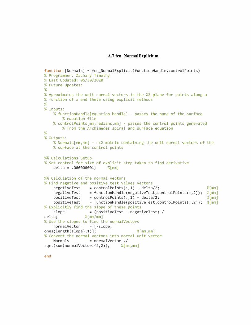
A.7 fcn_NormalExplicit.m
function [Normals] = fcn_NormalExplicit(functionHandle,controlPoints) % Programmer: Zachary Timothy % Last Updated: 06/30/2020 % Future Updates: % % Aproximates the unit normal vectors in the XZ plane for points along a % function of x and theta using explicit methods % % Inputs: % functionHandle[equation handle] - passes the name of the surface % equation file % controlPoints[mm,radians,mm] - passes the control points generated % from the Archimedes spiral and surface equation % % Outputs: % Normals[mm,mm] - nx2 matrix containing the unit normal vectors of the % surface at the control points %% Calculations Setup % Set control for size of explicit step taken to find derivative delta = .000000001; %[mm] %% Calculation of the normal vectors % Find negative and positive test values vectors negativeTest = controlPoints(:,1) - delta/2; %[mm] negativeTest = functionHandle(negativeTest,controlPoints(:,2)); %[mm] positiveTest = controlPoints(:,1) + delta/2; %[mm] positiveTest = functionHandle(positiveTest,controlPoints(:,2)); %[mm] % Explicitly find the slope of these points slope = (positiveTest - negativeTest) / delta; %[mm/mm] % Use the slopes to find the normalVectors normalVector = [-slope, ones(length(slope),1)]; %[mm,mm] % Convert the normal vectors into normal unit vector Normals = normalVector ./ sqrt(sum(normalVector.^2,2)); %[mm,mm] end
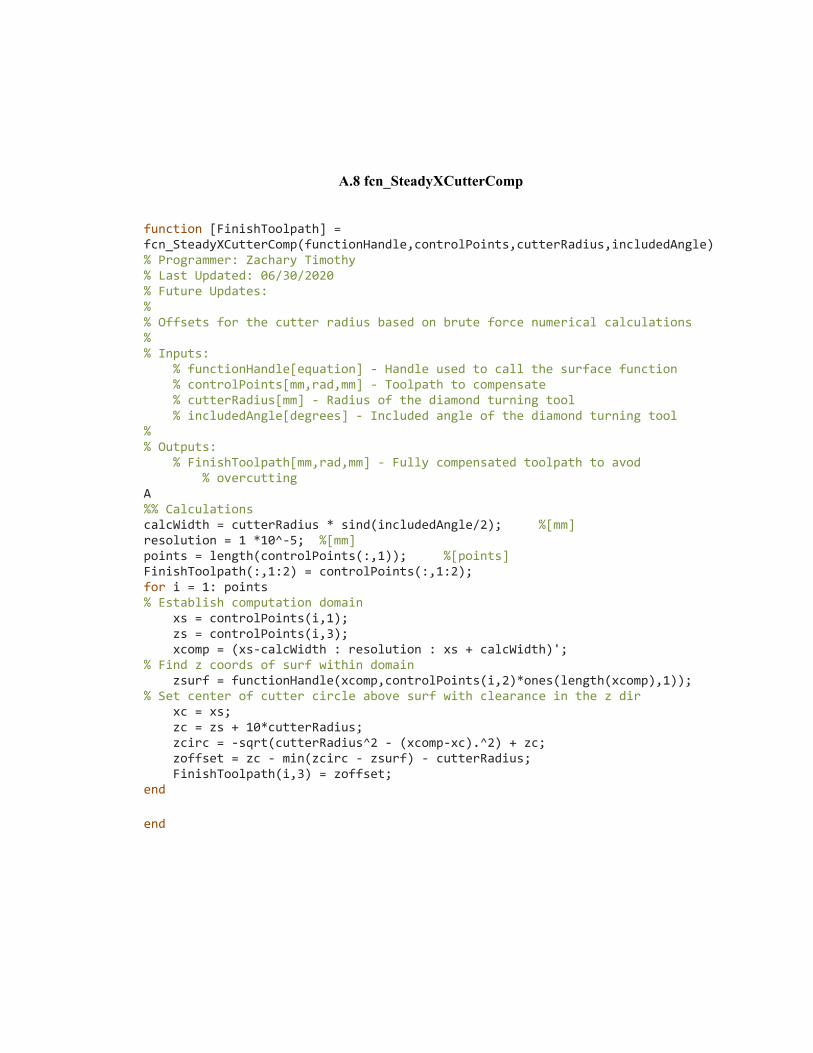
A.8 fcn_SteadyXCutterComp
function [FinishToolpath] = fcn_SteadyXCutterComp(functionHandle,controlPoints,cutterRadius,includedAngle) % Programmer: Zachary Timothy % Last Updated: 06/30/2020 % Future Updates: % % Offsets for the cutter radius based on brute force numerical calculations % % Inputs: % functionHandle[equation] - Handle used to call the surface function % controlPoints[mm,rad,mm] - Toolpath to compensate % cutterRadius[mm] - Radius of the diamond turning tool % includedAngle[degrees] - Included angle of the diamond turning tool % % Outputs: % FinishToolpath[mm,rad,mm] - Fully compensated toolpath to avod % overcutting A %% Calculations calcWidth = cutterRadius * sind(includedAngle/2); %[mm] resolution = 1 *10^-5; %[mm] points = length(controlPoints(:,1)); %[points] FinishToolpath(:,1:2) = controlPoints(:,1:2); for i = 1: points % Establish computation domain xs = controlPoints(i,1); zs = controlPoints(i,3); xcomp = (xs-calcWidth : resolution : xs + calcWidth)'; % Find z coords of surf within domain zsurf = functionHandle(xcomp,controlPoints(i,2)*ones(length(xcomp),1)); % Set center of cutter circle above surf with clearance in the z dir xc = xs; zc = zs + 10*cutterRadius; zcirc = -sqrt(cutterRadius^2 - (xcomp-xc).^2) + zc; zoffset = zc - min(zcirc - zsurf) - cutterRadius; FinishToolpath(i,3) = zoffset; end end

A.9 fcn_GoldenSteadyXCutterComp
function [FinishToolpath] = fcn_GoldenSteadyXCutterComp(functionHandle,controlPoints,cutterRadius,includedAngle) % Programmer: Zachary Timothy % Last Updated: 06/30/2020 % Future Updates: Tilted zero angle rake tools? % % Offsets for the cutter radius by offsetting strictly in the z direction. % The cutter edge is compared to the surface numerically by using a binary % golden section serach method to find the minimum distance between. % % Inputs: % functionHandle[equation] - Handle used to call the surface function % controlPoints[mm,rad,mm] - Toolpath to compensate % cutterRadius[mm] - Radius of the diamond turning tool % includedAngle[degrees] - Included angle of the diamond turning tool % % Outputs: % FinishToolpath[mm,rad,mm] - Fully compensated toolpath to avoid % overcutting %% Calculations % % % Dev test code flag, only use when using the specific test for this % % % function. Set = 1 to include the graphs % % flag = 0; % Golden number inverse G = (sqrt(5)-1)/2; %[] % Find length of dataset points = length(controlPoints(1)); %[points] % Accuracy level small = 1*10^-10; %[mm] % Create xmin vector xmin = controlPoints(:,1) - cutterRadius*ones(points,1); %[mm] % Create xmax vector xmax = controlPoints(:,1) + cutterRadius*ones(points,1); %[mm] % Calc x0 vector x0 = xmin + (1-G) .* (xmax-xmin); %[mm] % Calc x1 vector x1 = xmin + G .* (xmax - xmin); %[mm] % Calc v0 and v1 v0 = -fcn_CutterEdge(controlPoints,x0,cutterRadius,includedAngle) + functionHandle(x0,controlPoints(:,2)); %[mm] v1 = -fcn_CutterEdge(controlPoints,x1,cutterRadius,includedAngle) + functionHandle(x1,controlPoints(:,2)); %[mm] % Initial condition check
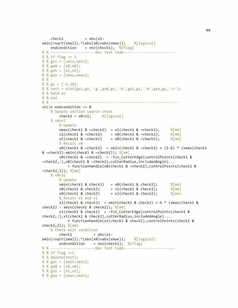
99
check1 = abs(x1-xmin)>sqrt(small).*(abs(x0)+abs(xmax)); %[logical] endcondition = nnz(check1); %[flag] % % ---------------------Dev Test Code------------------------ % % if flag == 1 % % gxi = [xmin,xmin]; % % gx0 = [x0,x0]; % % gx1 = [x1,x1]; % % gxa = [xmax,xmax]; % % % % gz = [-5,30]; % % test = plot(gxi,gz,':g',gx0,gz,':b',gx1,gz,':b',gxa,gz,':r'); % % hold on % % end % % ------------------------------------------------------------ while endcondition ~= 0 % Update section search check check2 = v0<v1; %[logical] % v0>v1 % Update xmax(check1 & ~check2) = x1(check1 & ~check2); %[mm] v1(check1 & ~check2) = v0(check1 & ~check2); %[mm] x1(check1 & ~check2) = x0(check1 & ~check2); %[mm] % Recalc v0 x0(check1 & ~check2) = xmin(check1 & ~check2) + (1-G) * (xmax(check1 & ~check2)-xmin(check1 & ~check2)); %[mm] v0(check1 & ~check2) = -fcn_CutterEdge(controlPoints(check1 & ~check2,:),x0(check1 & ~check2),cutterRadius,includedAngle)... + functionHandle(x0(check1 & ~check2),controlPoints(check1 & ~check2,2)); %[mm] % v0<v1 % Update xmin(check1 & check2) = x0(check1 & check2); %[mm] v0(check1 & check2) = v1(check1 & check2); %[mm] x0(check1 & check2) = x1(check1 & check2); %[mm] % Recalc x1 and v1 x1(check1 & check2) = xmin(check1 & check2) + G * (xmax(check1 & check2) - xmin(check1 & check2)); %[mm] v1(check1 & check2) = -fcn_CutterEdge(controlPoints(check1 & check2,:),x1(check1 & check2),cutterRadius,includedAngle)... + functionHandle(x1(check1 & check2),controlPoints(check1 & check2,2)); %[mm] % Check exit condition check1 = abs(x1-xmin)>sqrt(small).*(abs(x0)+abs(xmax)); %[logical] endcondition = nnz(check1); %[flag] % % ---------------------Dev Test Code------------------------ % % if flag ==1 % % delete(test); % % gxi = [xmin,xmin]; % % gx0 = [x0,x0]; % % gx1 = [x1,x1]; % % gxa = [xmax,xmax];
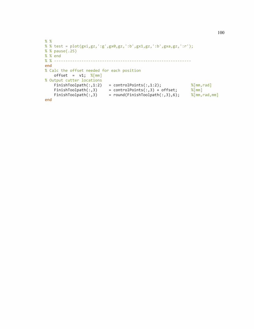
100
% % % % test = plot(gxi,gz,':g',gx0,gz,':b',gx1,gz,':b',gxa,gz,':r'); % % pause(.25) % % end % % ------------------------------------------------------------ end % Calc the offset needed for each position offset = v1; %[mm] % Output cutter locations FinishToolpath(:,1:2) = controlPoints(:,1:2); %[mm,rad] FinishToolpath(:,3) = controlPoints(:,3) + offset; %[mm] FinishToolpath(:,3) = round(FinishToolpath(:,3),6); %[mm,rad,mm] end

A.10 fcn_CutterEdge
function [toolEdgeZ] = fcn_CutterEdge(controlPoints,x,cutterRadius,includedAngle) % Programmer: Zachary Timothy % Last Updated: 08/06/2020 % Future Updates: % % Takes control points for the cutter tip locations and the cutter % information to give the z coordinate along the cutter edge at coordinates % x respectively. Only calculates over the diameter of the cutter radius. % % Inputs: % controlPoints[mm,rad,mm] - locations of the cutter tips along the % spiral drive path % x[mm] - vector containing the respective x locations, to the control % points, to find the z coordinate of % cutterRadius[mm] - radius of the diamond turning tool % includedAngle[degrees] - included angle of the diamond turning tool % % Outputs % toolEdgeZ[mm] - z coordinate of the tool edge at the given x % coordinate %% Calculations % Modify included angle for calculations includedAngle = 180-includedAngle; %[degrees] % Find the number of points to be calculated points = length(controlPoints(:,1)); %[] % Initialize tool edge matrix toolEdgeZ = zeros(points,1); %[mm] % Find the half width of the portion along the curved edge curvedRadius = cutterRadius * sind(includedAngle/2); %[mm] % Set the upper and lower limits of calculation curveMin = controlPoints(:,1) - curvedRadius*ones(points,1); %[mm] curveMax = controlPoints(:,1) + curvedRadius*ones(points,1); %[mm] % Error check for any values of calc domain outRange = x<controlPoints(:,1)-cutterRadius | x>controlPoints(:,1)+cutterRadius; %[logical] if nnz(outRange) > 1 warning('Input tool x is beyond the appropriate calculation range') end % Create logical vectors for the three regions of the cutter edge lowTest = x < curveMin; %[logical] lowPoints = nnz(lowTest); %[points] highTest = x > curveMax; %[logical] highPoints = nnz(highTest); %[points] midTest = ~(lowTest|highTest); %[logical] % X within curved portion of cutter

102
toolEdgeZ(midTest) = cutterRadius + controlPoints(midTest,3) - sqrt(cutterRadius^2 ... - (controlPoints(midTest,1)-x(midTest)).^2); %[mm] % X lower than curved portion toolEdgeZ(lowTest) = controlPoints(lowTest,3) + (cutterRadius - sqrt(cutterRadius^2-curvedRadius^2))*... ones(lowPoints,1) + (controlPoints(lowTest,1)-curvedRadius*ones(lowPoints,1)-x(lowTest))*tand(includedAngle/2); %[mm] % X hihgher than curved portion toolEdgeZ(highTest) = controlPoints(highTest,3) + (cutterRadius - sqrt(cutterRadius^2-curvedRadius^2))*... ones(highPoints,1) + (-controlPoints(highTest,1)-curvedRadius*ones(highPoints,1)+x(highTest))*tand(includedAngle/2); %[mm] end
A.11 fcn_MachiningSetup
function [FinishBase,RoughBase,offset] = fcn_MachiningSetup( finishControlPoints,roughControlPoints,roughDepth,finishDepth,finishPasses, roughPasses) % Programmer: Zachary Timothy % Last Updated: 07/08/2020 % Future Updates: % % Offsets the set of control points to all be below the 'zero' surface by % at least one rough and finish pass % % Inputs: % finishControlPoints[mm,rad,mm] - values of the finish control points % roughControlPoints[mm,rad,mm] - values of the rough control points % roughDepth[mm] - height to be used for roughing passes % finishDepth[mm] - height to be used for finishing passes % finishPasses[passes] - total number of desired finishing passes % roughPasses[passes] - total number of desired roughing passes % % Outputs: % FinishBase[mm,rad,mm] - finalized coordinates of the finishing base % points % RoughBase[mm,rad,mm] - finalized coordinates of the roughing base % points % offset[mm] - value needed later in entry path generation %% Calculations % Find the max z coordinate of the toolpath maxHeight = max(finishControlPoints(:,3)); %[mm] % Create an offset equal to the max height, finish depth, and rough depth % combined offset = roughDepth*roughPasses + maxHeight + finishDepth * finishPasses; %[mm] % Create the offset matrices finishOffset = [zeros(length(finishControlPoints(:,3)),2),ones(length(finishControlPoints(:,3)),1)*offset]; %[mm] roughOffset = [zeros(length(roughControlPoints(:,3)),2),ones(length(roughControlPoints(:,3)),1)*offset]; %[mm] % Offset the tool paths FinishBase = finishControlPoints - finishOffset; %[mm] RoughBase = roughControlPoints - roughOffset; %[mm] % Reset offset for later calcs offset = roughDepth*roughPasses + maxHeight; %[mm] end

A.12 fcn_FinishingPasses
function [FinishToolpaths] = fcn_FinishingPasses(finishBase,finishDepth, finishPasses) % Programmer: Zachary Timothy % Last Updated: 07/15/2020 % Future Updates: % % Adds the respective offsets to the finish base points to create the coordinates for the finishing passes % % Inputs: % finishBase[mm,rad,mm] - Matrix containing the correct offset coordinates of the finishing base points % finishDepth[mm] - Height to be used for finishing passes % finishPasses[passes] - Total number of desired finishing passes % % Outputs: % FinishToolpaths[mm,rad,mm] - Complete set of finishing cutting path coordinates %% Calculations % Preallocate matrix for speed FinishToolpaths = zeros(length(finishBase(:,1)),3,finishPasses); % Offset each layer for the finish passes for i = 1 :finishPasses FinishToolpaths(:,1:2,i) = finishBase(:,1:2); FinishToolpaths(:,3,i) = finishBase(:,3) + (finishPasses-i) * finishDepth; end end
A.13 fcn_RoughingPasses
function [RoughPasses,passes] = fcn_RoughingPasses(roughDepth,finishDepth,finishBase,finishPasses,roughBase) % Programmer: Zachary Timothy % Last Updated: 07/15/2020 % Future Updates: Add ability for input of precut stock % % Creates a 3d matrix of the coordinates for the roughing passes. % % Inputs: % roughDepth[mm] - height to be used for roughing passes % finishDepth[mm] - height ot be used for finishing passes % finishBase[mm] - finalized coordinates of the finish base points % finishPasses[passes] - number of finishing passes % roughBase[mm,rad,mm] - coordinates for the roughing base points % % Outputs: % RoughPasses[mm,rad,mm][passes] - 3d matrix with the coordinates for % each roughing pass % passes[passes] - calculated number of roughing passes %% Calculations % Find the lowest z coordinate of the finish toolpath maxDepth = abs(min(finishBase(:,3))); %[mm] % Find the height needed for the finish pass(es) finishLayer = finishPasses * finishDepth; % Find the number of rough passes needed passes = ceil(round((maxDepth - finishLayer) / roughDepth,6)); %[passes] % Find the number of points for each spiral %[points] roughPoints = length(roughBase(:,3)); % Initialize the rough passes matrix RoughPasses = zeros(roughPoints,3,passes); %[empty] for i = 1: passes RoughPasses(:,1:2,i) = roughBase(:,1:2); %[mm,rad] end % Setup stock vector stock = zeros(roughPoints,1); %[mm] % Start the pass calcs for i = 1:passes % Calculate the height left to be roughed stockRemain = stock - roughBase(:,3,1); %[mm] % Calculate what the cut height for each point is cut = fcn_CutCalc(stockRemain,roughDepth,finishLayer); %[mm] % Update the stock stock = stock - cut; %[mm] % Set the roughing pass cordinates equal to the stock RoughPasses(:,3,i) = stock; %[mm,rad,mm]

106
end end
A.14 fcn_CutCalc
function [Cut] = fcn_CutCalc(stockRemain,roughDepth,finishLayer) % Programmer: Zachary Timothy % Last Updated: 07/08/2020 % Future Updates: % % Calculates the appropriate height of rough cut based on how much stock % remains to the finish pass coordinates for a single rough pass % % Inputs: % stockRemain[mm] - vector containing how much stock is left at each % control point % roughDepth[mm] - desired height for roughing passes % finishDepth[mm] - desired height for finishing passes % % Outputs: % Cut[mm] - vector with the appropriate cut height for each control % point %% Error Checking %% Calculations % Find the number of points for each pass points = length(stockRemain); %[points] % Initialize the cut vector Cut = zeros(points,1); %[mm] % Begin point by point comparison for i = 1:points % Compare the stock remain of the point if stockRemain(i) >= roughDepth + finishLayer % Enough stock remains for a full rough depth pass Cut(i) = roughDepth; %[mm] elseif stockRemain(i) < roughDepth + finishLayer && stockRemain(i) > finishLayer % Enough stock remains for a partial rough pass Cut(i) = stockRemain(i) - finishLayer; %[mm] elseif stockRemain(i) == finishLayer % At finishing height, don't cut Cut(i) = 0; %[mm] end end end

A.15 fcn_InverseTimeCalcs
function [FeedRate] = fcn_InverseTimeCalcs(spindleSpeed,toolPaths) % Programmer: Zachary Timothy % Last Updated: 07/09/2020 % Future Updates: % % Finds the feedrate in units of seconds, rounded to the nearest % millisecond for each point to be used in inverse time mode G93 when % diamond turning. % % Inputs: % spindleSpeed[rev/min] - desired spindle speed whilst turning % finishPass[mm] - finalized coordinates of the finishing pass % % Outputs: % feedRate[seconds] - feedrate to be used for the f word in G93 mode %% Internal Variables % Machine max linear velocity allowed [maxSpeed,maxAccel,maxSpeedScale] = var_internal('InverseTimeCalcs'); %[mm/s] %% Calculations % Apply scaling factor to max Speed % maxSpeed = maxSpeed * maxSpeedScale; % Convert spindle speed spindleSpeed = spindleSpeed * 2*pi / 60; %[rad/sec] % Initialize deltaPath as first theta change deltaPath = toolPaths(2,2,:) - toolPaths(1,2,:); % Find the change in theta for each point deltaPath = toolPaths(2:end,:,:) - toolPaths(1:end-1,:,:); %[mm,rad,mm] % Find the initial feedrate by dividing change in theta by speed of theta FeedRate = deltaPath(:,2,:) / spindleSpeed; %[seconds] FeedRate = [FeedRate(1,:,:);FeedRate]; % Check for below 1 ms feedSmall = FeedRate < .001; %[logical] FeedRate(feedSmall) = .001; %[mm] for i = 1:size(FeedRate,3) tempFeed = max(FeedRate(:,1,i)); % Velocity Check tempSpeed = gradient(toolPaths(:,3,i),tempFeed); % Check if speed goes over scale = tempSpeed./maxSpeed; scale = max(abs(scale)); tempFeed(scale>1) = tempFeed(scale>1).*scale(scale>1); % Accel Check tempAccel = gradient(tempSpeed,tempFeed);

109
% Check if accel goes over scale = tempAccel(:,1)./maxAccel; scale = max(scale); tempFeed(scale>1) = tempFeed(scale>1).*scale(scale>1); % For each pass, set feedRate to be maximum FeedRate(:,1,i) = ones(size(toolPaths,1),1) * tempFeed; end % Round up to nearest millisecond FeedRate = ceil(FeedRate*1000)/1000; end

A.16 fcn_Retraction
function [Retract] = fcn_Retraction(passes,maxSpeed,retractHeight) % Programmer: Zachary Timothy % Last Updated: 08/31/2020 % Future Updates: switch to constant velocity if over vmax instead of % slowed polynomial % % Creates the retraction paths after each cut to program for continuous % paths using polynomial trajectories. Checks the following for limit % crossings: linear velocity, linear acceleration, rotational acceleration, % and spindle power. % % Inputs: % passes[mm,rad,mm,seconds][pass] - 3D matrix containg the locaitons of % the cutting passes % maxSpeed[mm/s] - commanded max travel speed from input seciton % retractHeight[mm] - z coordinate to retract to after each pass % % Outputs: % Retract[mm,rad,mm,seconds] - toolpath coordinates for retractions % after each pass %% Internal Variables [maxVel,maxAccel,maxAngularAccel,maxPower,momentOfInertia,maxAccelMaragin] = var_internal('Retraction'); %% Calculations % Check rapid travel speed to ensure it is within machine limits maxSpeed = min(maxSpeed,maxVel); %[mm/s] % Find linear speed and locations at last points of curves z0 = passes(end,3,:); %[mm] v0 = (passes(end-1,3,:)-passes(end,3,:))./passes(end,4,:); %[mm/s] % Find retraction distance delZ = retractHeight - z0; %[mm] % Calc time for retraction based on polynomial trajectory aMax = maxAccel*maxAccelMaragin; %[mm/s] linMoveTime(1,1,:) = -(2*v0 - 2^(1/2)*(2*v0.^2 + 3*aMax.*delZ).^(1/2))./aMax; %[seconds] % Check max speeds vMax = ((2*v0.^2 + 3*aMax.*delZ).*(3*aMax.*delZ + 4*v0.^2 + 2*v0.*(4*v0.^2 +... 6*aMax.*delZ).^(1/2)))./(2*(4*v0.^3 + 2^(1/2)*(2*v0.^2 + 3*aMax.*delZ).^(3/2) + 9*aMax.*delZ.*v0)); %[mm/s] linScale = vMax./maxSpeed; %[scale] velCheck = linScale > 1; %[logical] % Adjust if necessary linMoveTime(velCheck) = linMoveTime(velCheck).*linScale(velCheck); %[seconds] % % % Recheck velocity (Dev)

111
% % vMax(velCheck) = (3.*delZ(velCheck)-linMoveTime(velCheck).*v0(velCheck)).^2./(3.*linMoveTime(velCheck)... % % .*(2.*delZ(velCheck)-linMoveTime(velCheck).*v0(velCheck))); %[m/s] % Setup timing parameters tStep = passes(end,4,:); %[seconds] linSteps = ceil(linMoveTime./tStep); %[seconds] rotMoveTime = linMoveTime; %[seconds] % Find initial rotary information theta0 = passes(end,2,:); %[rad] w0 = (passes(end,2,:)-passes(end-1,2,:))./passes(end,4,:); %[rad/s] % Check angular acceleration limit alphMax = w0(1,1,:)./rotMoveTime(1,1,:); %[rad/s^2] alphScale = alphMax/maxAngularAccel; %[scale] alphCheck = alphScale>1; %[logical] % Adjust if necessary rotMoveTime(alphCheck) = rotMoveTime(alphCheck).*alphScale(alphCheck); %[seconds] % Check spindle power limit powerMax = w0(1,1,:).^2.*momentOfInertia./rotMoveTime; %[W] powerScale = powerMax./maxPower; %[scale] powerCheck = powerScale>1; %[logical] % Adjust if necessary rotMoveTime(powerCheck) = rotMoveTime(powerCheck).*powerScale(powerCheck); %[seconds] % Find total number of steps needed steps = ceil(rotMoveTime./tStep); %[steps] % Assemble retraction matrices based on polynomial projections for i = 1:size(passes,3) % Create time vector t{i} = [1:steps(i)-1]'; t{i} = t{i}*tStep(1,1,i); % Create empty z vector z = []; % for j = 1:steps(i)-1 % t{i}(j,1) = j.*tStep(1,1,i); %[seconds] % end j = steps(i)-1; % Assemble time vector t{i} = [t{i}(:,1);rotMoveTime(1,1,i)]; %[seconds] % Create the x vector x = ones(j+1,1)*passes(end,1,i); %[mm] % Create theta vector theta = -w0(1,1,i)./(2.*rotMoveTime(1,1,i)).*t{i}(:,1).^2 + w0(1,1,i).*t{i}(:,1) + theta0(1,1,i); %[rad] % Create z vector if ~velCheck(i) % Standard trajectory z(1:linSteps(i)-1,1) = -(4.*t{i}(1:linSteps(i)-1).^3.*v0(1,1,i).^3 - 54.*delZ(1,1,i).^2.*z0(1,1,i)... - 54.*delZ(1,1,i).^2.*t{i}(1:linSteps(i)-1).*v0(1,1,i) - 27.*aMax.*delZ(1,1,i).^2.*t{i}(1:linSteps(i)-1).^2 ...

112
+ 2.^(1/2).*t{i}(1:linSteps(i)-1).^3.*(2.*v0(1,1,i).^2 + 3.*aMax.*delZ(1,1,i)).^(3/2) + 9.*aMax.*delZ(1,1,i).* ... t{i}(1:linSteps(i)-1).^3.*v0(1,1,i))./(54.*delZ(1,1,i).^2); %[mm] else % Maxed velocity trajectory z(1:linSteps(i)-1,1) = z0(1,1,i)+t{i}((1:linSteps(i)-1),1).*v0(1,1,i)+(t{i}((1:linSteps(i)-1),1).^2.* ... (3.*delZ(1,1,i)-2.*linMoveTime(1,1,i).*v0(1,1,i)))./linMoveTime(1,1,i).^2-(t{i}((1:linSteps(i)-1),1).^3.* ... (2.*delZ(1,1,i) - linMoveTime(1,1,i).*v0(1,1,i)))./linMoveTime(1,1,i).^3; %[mm] end % Set z for spindle cool down z(linSteps(i):steps(i)) = retractHeight; %[mm] % Set first t value as 0 t{i}(1:end+1) = [0;t{i}(:,1)]; %[seconds] % Find feedrates f = t{i}(2:end,1)-t{i}(1:end-1); %[seconds] % Round to nearest milisecond f = round(f*1000)/1000; %[seconds] % Adjust last time step f(end) = tStep(1,1,i); % Round small values to one milisecond f(f<.001) = .001; %[seconds] % Create retraction matrix Retract{i} = [x,theta,z,f]; %[mm,radians,mm,seconds] end end

A.17 fcn_EntryPasses
function [EntryPasses] = fcn_EntryPasses(toolPath,feedRate,cutterRadius,surfaceFcn,workpieceRadius) % Programmer: Zachary Timothy % Last Updated: 09/22/2020 % Future Updates: % % Creates a specified number of rotations as an approach to the cutting % passes. Works by offsetting the outermost full rotation of the cutting % pass in the radial direciton. Uses a polynomial trajectory for smooth % start up % % Inputs: % toolPath[mm,rad,mm] - Positions of cutting toolpaths % feedRate[mm/rev] - Feedrate for the x axis in spiral generation % res[degrees] - Angular resoluiton of the archimedes spirral % cutterRadius[mm] - Radius of the diamond turning tool % surfaceFcn[handle] - Handle to call the surface funciton % workpieceRadius[mm] - radius of the workpiece % Outputs % EntryPasses[mm,rad,mm] - Entry pass matrix for smooth transitions %% Internal Variables [accelScale,maxAngularAccel,entryLength] = var_internal('EntryPasses'); %% Calculations % Find the total number of passes passes = size(toolPath,3); %[passes] % Path conditions aMax = accelScale*maxAngularAccel; %[rad/s^2] % Take standard angular spacing of entry to be first of path delTheta = toolPath(2,2,:); %[radians] % Take standard feedrate to be of first point in path delT = toolPath(1,4,:); wf = delTheta./delT; % Polynomial start up parameters A = -(4*aMax.^3)./(27*wf.^2); %[rad/s^4] B = 4*aMax.^2./(9*wf); %[rad/s^2] totalTime = (3*wf)./(2*aMax); %[seconds] totalTheta = A.*totalTime.^4 + B.*totalTime.^3; %[radians] % Find the number of rotations needed for the entry pass, round up for safety entryRotations = ceil(entryLength/feedRate); %[rotations] % Check passes are enough for smooth start up scale = max(totalTheta)./(entryRotations*2*pi); %[scale] entryRotations(scale>1) = ceil(totalTheta(scale>1)/(2*pi)); %[rotations] % Check number of passes won't cause tool interference early safety = cutterRadius*2/feedRate; %[]

114
scale = safety./entryRotations; %[] entryRotations(scale>1) = ceil(scale*entryRotations); %[rotations] for i = 1:passes % Ramp up period of entry rampTime = [0:delT(1,1,i):totalTime(1,1,i)]'; %[seconds] thetaRamp = A(1,1,i).*rampTime.^4 + B(1,1,i).*rampTime.^3; %[rad] rRamp = workpieceRadius + entryRotations*feedRate - feedRate.*thetaRamp./(2*pi); %[mm] fRamp = ones(size(thetaRamp,1),1)*delT(1,1,i); %[seconds] % Transition thetaTrans = (delTheta(1,1,i)-rem(thetaRamp(end),delTheta(1,1,i))); %[rad] thetaRamp = thetaRamp + thetaTrans; %[rad] rTrans = -feedRate.*thetaTrans./(2*pi); %[mm] rRamp = rRamp + rTrans; %[mm] % Steady portion thetaSteady = [thetaRamp(end)+delTheta(1,1,i):delTheta(1,1,i):entryRotations*2*pi-delTheta(1,1,i)]'; %[rad] rSteady = workpieceRadius + entryRotations*feedRate - feedRate.*(thetaSteady./(2*pi)); %[mm] fSteady = delT(1,1,i)*ones(size(thetaSteady,1),1); %[seconds] % Assign entry Pass EntryPasses{i} = [rRamp, thetaRamp, fRamp rSteady, thetaSteady, fSteady]; %[mm,rad,seconds] z = surfaceFcn(workpieceRadius, EntryPasses{i}(:,2)); %[mm] EntryPasses{i} = [EntryPasses{i}(:,1:2),z,EntryPasses{i}(:,3)]; %{pass}[mm,rad,mm,seconds] end end
A.18 fcn_EntryOffset
function [EntryPasses] = fcn_EntryOffset(toolPath,EntryPasses,offset,tag,surfaceFcn) % Programmer: Zachary Timothy % Last Updated: 11/16/2020 % Future Updates: % % Adds the Z offset to finalize the coordinaes for the entry passes % % Inputs: % EntryPasses{pass}[mm,rad,mm] - entry pass coordinates % offset[mm] - offset for finish boundary layer % tag[string] - identifier for rough/finish % surfaceFcn[handle] - handle to call surface function % % Outputs: % EntryPasses{pass}[mm,rad,mm] - offset entry pass coordinates %% Calculations for i = 1:size(toolPath,3) if strcmp(tag,'Finish') depth = surfaceFcn(toolPath(1,1,i),toolPath(1,2,i)) - toolPath(1,3,i); %[mm] EntryPasses{i}(:,3) = EntryPasses{i}(:,3) - depth; %{pass}[mm,rad,mm] else EntryPasses{i}(:,3) = EntryPasses{i}(:,3) - offset; %{pass}[mm,rad,mm] maxDepth = min(toolPath(:,3,i)); %[mm] index = EntryPasses{i}(:,3) < maxDepth; %[logical] EntryPasses{i}(index,3) = maxDepth; %{pass}[mm,rad,mm] end end

A.19 fcn_ConvertC
function [ROUGH,FINISH] = fcn_ConvertC(ROUGH,FINISH) % Programmer: Zachary Timothy % Last Updated: 09/23/2020 % Future Updates: Include all parts of toolpaths - (retract when complete) % % Converts all coordinates in radians to degrees % % Inputs: % ROUGH.toolPaths[mm,rad,mm] - 3 dimensional matrix containing the % coordinates for all the roughing passes % ROUGH.entries[mm,rad,mm] - 3 dimensional matrix containing the % coordinates for all entry paths into the roughing passes % FINISH.toolPaths[mm,rad,mm] - 3 dimensional matrix containing the % coordinates for all the finishing passes % FINISH.entries[mm,rad,mm] - 3 dimensional matrix containing the % coordinates for all entry paths into the finishing passes % % Outputs: % ROUGH.toolPaths[mm,deg,mm] - 3 dimensional matrix containing the % coordinates for all the roughing passes % ROUGH.entries[mm,deg,mm] - 3 dimensional matrix containing the % coordinates for all entry paths into the roughing passes % FINISH.toolPaths[mm,deg,mm] - 3 dimensional matrix containing the % coordinates for all the finishing passes % FINISH.entries[mm,deg,mm] - 3 dimensional matrix containing the % coordinates for all entry paths into the finishing passes %% Calculations ROUGH.toolPaths(:,2,:) = rad2deg(ROUGH.toolPaths(:,2,:)); %[degrees] for i = 1:ROUGH.passes ROUGH.retract{i}(:,2) = rad2deg(ROUGH.retract{i}(:,2)); %[degrees] ROUGH.entries{i}(:,2) = rad2deg(ROUGH.entries{i}(:,2)); %[degrees] end FINISH.toolPaths(:,2,:) = rad2deg(FINISH.toolPaths(:,2,:)); %[degrees] for i = 1:FINISH.passes FINISH.retract{i}(:,2) = rad2deg(FINISH.retract{i}(:,2)); %[degrees] FINISH.entries{i}(:,2) = rad2deg(FINISH.entries{i}(:,2)); %[degrees] end end
A.20 fcn_PathAssembly
function [ROUGH,FINISH,SETUP] = fcn_PathAssembly(ROUGH,FINISH,SETUP) % Programmer: Zachary Timothy % Last Updated: 07/20/2020 % Future Updates: % % Goes through an iterative algorithm to make the total inteded toolpath % continuous w.r.t. the c axis % % Inputs/Outputs: % ROUGH % FINISH % SETUP %% Calculation % Initialize offset = 0; %[] SETUP.totalTime = 0; %[] for i = 1:ROUGH.passes % Entry starts at 0, offset by most recent value ROUGH.entries{i}(:,2) = ROUGH.entries{i}(:,2)+offset; %[degrees] % Set approach position ROUGH.approach(1,:,i) = [ROUGH.entries{i}(1,1:2),SETUP.retractHeight]; %[mm,degrees,mm] % Update offset to be end of entry offset = 360-mod(ROUGH.entries{i}(end,2),360)+ROUGH.entries{i}(end,2); %[degrees] % Toolpath begins at 0, offset by most recent value ROUGH.toolPaths(:,2,i) = ROUGH.toolPaths(:,2,i) + offset; %[degrees] % Retract picks up where toolPath leaves, use same offset as toolpath ROUGH.retract{i}(:,2) = ROUGH.retract{i}(:,2) + offset; %[degrees] % Update offset to be end of retract offset = ROUGH.retract{i}(end,2) + (360-mod(ROUGH.retract{i}(end,2),360)); %[degrees] % Assemble path ROUGH.totalPath{i}(:,:) = [ROUGH.entries{i}(:,:);ROUGH.toolPaths(:,:,i);ROUGH.retract{i}(:,:)]; %[mm,rad,mm] ROUGH.totalPath{i}(:,:) = round(ROUGH.totalPath{i}(:,:),8); %[mm,rad,mm] % Round to 360 ROUGH.totalPath{i}(:,2) = rem(ROUGH.totalPath{i}(:,2),360); %[rad] ROUGH.entries{i}(:,2) = rem(ROUGH.entries{i}(:,2),360); %[rad]

118
% Calculate time for each pass and update total time SETUP.totalTime = SETUP.totalTime + sum(ROUGH.totalPath{i}(:,4)); %[seconds] end ROUGH.approach(1,2,:) = rem(ROUGH.approach(1,2,:),360); for i = 1:FINISH.passes % Entry starts at 0, offset by most recent value FINISH.entries{i}(:,2) = FINISH.entries{i}(:,2)+offset; %[degrees] % Set approach position FINISH.approach(1,:,i) = [FINISH.entries{i}(1,1:2),SETUP.retractHeight]; %[mm,degrees,mm] % Update offset to be end of entry offset = 360-mod(FINISH.entries{i}(end,2),360)+FINISH.entries{i}(end,2); %[degrees] % Toolpath begins at 0, offset by most recent value FINISH.toolPaths(:,2,i) = FINISH.toolPaths(:,2,i) + offset; %[degrees] % Retract picks up where toolPath leaves, use same offset as toolpath FINISH.retract{i}(:,2) = FINISH.retract{i}(:,2) + offset; %[degrees] % Update offset to be end of retract offset = FINISH.retract{i}(end,2) + (360-mod(FINISH.retract{i}(end,2),360)); %[degrees] % Assemble path FINISH.totalPath{i}(:,:) = [FINISH.entries{i}(:,:);FINISH.toolPaths(:,:,i);FINISH.retract{i}(:,:)]; %[mm,rad,mm] FINISH.totalPath{i}(:,:) = round(FINISH.totalPath{i}(:,:),8); %[mm,rad,mm] % Round to 360 FINISH.totalPath{i}(:,2) = rem(FINISH.totalPath{i}(:,2),360); %[rad] FINISH.entries{i}(:,2) = rem(FINISH.entries{i}(:,2),360); %[rad] % Calculate time for each pass and update total time SETUP.totalTime = SETUP.totalTime + sum(FINISH.totalPath{i}(:,4)); %[seconds] end FINISH.approach(1,2,:) = rem(FINISH.approach(1,2,:),360); %[rad] SETUP.totalTime = seconds(SETUP.totalTime); %[seconds] SETUP.totalTime = minutes(SETUP.totalTime); %[seconds] SETUP.idealRms = .032*(FINISH.feedRate)^2 / ( SETUP.cutterRadius * SETUP.spindleSpeed^2)*10^6; %[mm] end

A.21 fcn_NCFileWrite
function [] = fcn_NCFileWrite(POST,SETUP,ROUGH,FINISH) % Programmer: Zachary Timothy % Last Updated: 07/15/2020 % Future Updates: % % Takes in the the coordinates for machinng and outputs a text file % containing the appropriate nc code. % % Inputs: % POST % SETUP % ROUGH % FINISH %% Internal Variables [coolantOn,coolantOff,gsafety,gend] = var_internal('NCFileWrite'); %% Program % Post processesing parameters rapidMoveRate = SETUP.maxMoveSpeed; %[mm/s] homePosition = [0,0,SETUP.retractHeight]; %[mm,degrees,mm] % ------------------------------------------------------------------------- % 1. File initialization % ------------------------------------------------------------------------- % Before using compute time, check to make sure the machine parameters are % okay fprintf('Surface parameters:\n\tEstimated cutting time: %.2f minutes\n\tEstimated Ideal Ra = %.2f nm\n\tRoughing Passes: %i \n',SETUP.totalTime,SETUP.idealRms,ROUGH.passes); userInput = input('Hit enter to continue if parameters are acceptable, type anything and hit enter to exit: ','s'); if strcmp('',userInput) % Continue else error('Terminating Program, machining parameters not within range') end % Check if file already exists fileID = fopen(POST.fileName); if fileID ~= -1 % Prompt user if okay to overwrite existing file userInput = input('File with this name already exist, press enter if okay to overwrite existing file or enter new file name:\n','s'); % Rename fileName if desired if strcmp('',userInput) % do nothing

120
else POST.fileName = [userInput,'.nc']; end end % Open file with read and write permission fileID = fopen(POST.fileName,'w+'); % ------------------------------------------------------------------------- % 2. Write file opening sequences % ------------------------------------------------------------------------- % Write starting symbol and Program number fprintf(fileID,'%%\r\nO%s\r\n',POST.programNumber); % Formatting lines spacer = '(--------------------------------------------------------------------------)\r\n'; % Opening comment section line1 = '(MasterFlash gcode developed for use in the PSU MDRL with the Moore UPL 350)\r\n'; line2 = '(The workpiece is assumed to already be faced and work coordinate in G54)\r\n'; line3 = '(Part Name = %s)\r\n'; line4 = '(Programmer = %s)\r\n'; line5 = '(Date = %s)\r\n\n'; line6 = '(Tool = %s\t\t\t\t\t)\r\n'; line7 = '(\tRadius = %.3f mm\t\t\t)\r\n'; line8 = '(\tClearance Angle = %i degrees)\r\n'; line9 = '(\tRake Angle = %i degrees\t\t)\r\n\n'; line10 = '(Workpiece Diameter = %f mm)\r\n'; opening = [spacer,line1,line2,line3,line4,line5,line6,line7,line8,line9,line10,spacer]; fprintf(fileID,opening,POST.partName,POST.programmer,date,SETUP.toolName,... SETUP.cutterRadius,SETUP.clearanceAngle,SETUP.rakeAngle,SETUP. workpieceRadius); % Path properties fprintf(fileID,'(Path parameters)\r\n'); fprintf(fileID,'\t(Expected time for machining is %.2f minutes)\r\n',SETUP.totalTime); fprintf(fileID,'\t(%i Roughing Passes)\r\n',ROUGH.passes); fprintf(fileID,'\t(%i Finishing Passes)\r\n\n',FINISH.passes); fprintf(fileID,'\t(Estimated ideal surface roughness: %.2f nm)\r\n',SETUP.idealRms); % Safety blocks safety = '(Safety Blocks)\r\n'; fprintf(fileID,[safety,gsafety]); % Setup Machine to begin running fprintf(fileID,'M78 (C-axis mode)\r\n'); fprintf(fileID,'G01 Z%f F%i\r\n',homePosition(3),rapidMoveRate); fprintf(fileID,'G01 X%f C%.5f\r\n\n',homePosition(1),homePosition(2)); % Begin roughing passes fprintf(fileID,[spacer,'(Begin roughing passes)\r\n']); approach = 'G01 X%f C%.5f Z%f F%i\r\n';

121
for i = 1:ROUGH.passes % Header fprintf(fileID,[spacer,'(Roughing Pass %i)\r\nG94 (Feed per Min)\r\n'],i); % Approach fprintf(fileID,approach,ROUGH.approach(1,:,i),rapidMoveRate); fprintf(fileID,approach,ROUGH.entries{i}(1,1:3),rapidMoveRate); % Inverse Time % % fprintf(fileID,'%s (Coolant On)\n',coolantOn); fprintf(fileID,'G01 G93 F%.3f \r\n',ROUGH.totalPath{i}(1,4)); fprintf(fileID,'X%f C%.5f Z%f \r\n',ROUGH.totalPath{i}(1,1:3)); for j = 2:size(ROUGH.totalPath{i}(:,1),1) if ROUGH.totalPath{i}(j,1) ~= ROUGH.totalPath{i}(j-1,1) fprintf(fileID,'X%f ',ROUGH.totalPath{i}(j,1)); end if ROUGH.totalPath{i}(j,2) ~= ROUGH.totalPath{i}(j-1,2) if mod(ROUGH.totalPath{i}(j,2),1) == 0 fprintf(fileID,'C%g ',ROUGH.totalPath{i}(j,2)); else fprintf(fileID,'C%.5f ',ROUGH.totalPath{i}(j,2)); end end if ROUGH.totalPath{i}(j,3) ~= ROUGH.totalPath{i}(j-1,3) fprintf(fileID,'Z%f ',ROUGH.totalPath{i}(j,3)); end if ROUGH.totalPath{i}(j,4) ~= ROUGH.totalPath{i}(j-1,4) % % fprintf(fileID,'F%.3f',ROUGH.totalPath{i}(j,4)); warning('Error occured in rough feedRates, check before continuing') end fprintf(fileID,'\r\n'); end % % fprintf(fileID,'%s (Coolant off)\n',coolantOff); end % Begin finishing passes fprintf(fileID,[spacer,'(Begin finishing passes)\r\n']); for i = 1:FINISH.passes % Header fprintf(fileID,[spacer,'(Finishing Pass %i)\r\nG94 (Feed per Min)\r\n'],i); % Approach fprintf(fileID,approach,FINISH.approach(1,:,i),rapidMoveRate); fprintf(fileID,approach,FINISH.entries{i}(1,1:3),rapidMoveRate); % Inverse Time fprintf(fileID,'G01 G93 F%.3f \r\n',FINISH.totalPath{i}(1,4)); fprintf(fileID,'X%f C%.5f Z%f \r\n',FINISH.totalPath{i}(1,1:3)); for j = 2:size(FINISH.totalPath{i}(:,1),1) if FINISH.totalPath{i}(j,1) ~= FINISH.totalPath{i}(j-1,1) fprintf(fileID,'X%f ',FINISH.totalPath{i}(j,1)); end if FINISH.totalPath{i}(j,2) ~= FINISH.totalPath{i}(j-1,2)

122
if mod(FINISH.totalPath{i}(j,2),1) == 0 fprintf(fileID,'C%g ',FINISH.totalPath{i}(j,2)); else fprintf(fileID,'C%.5f ',FINISH.totalPath{i}(j,2)); end end if FINISH.totalPath{i}(j,3) ~= FINISH.totalPath{i}(j-1,3) fprintf(fileID,'Z%f ',FINISH.totalPath{i}(j,3)); end if FINISH.totalPath{i}(j,4) ~= FINISH.totalPath{i}(j-1,4) % % fprintf(fileID,'F%.3f',FINISH.totalPath{i}(j,4)); warning('Error occured in finish feedRates, check before continuing') end fprintf(fileID,'\r\n'); end end % End of program lines fprintf(fileID,'(End of Tape)\r\n'); fprintf(fileID,'G94\r\n G01 Z10 F60\r\n'); fprintf(fileID,gend); % Close the file program fclose(fileID); end

A.22 fcn_ToolOptimization
function [] = fcn_ToolOptimization(cutterRadius,includedAngle,surfaceFunction,workPieceRadius,clearanceAngle,controlPoints) % Programmer: Zachary Timothy % Last Updated: 09/03/2020 % Future Updates: Hybrid? % % Sub function to the algorithms for doing tool geometry checks and % optimizations %% Checks % Included angle maxIncludedAngle = fcn_IncludedAngleCheck(surfaceFunction,controlPoints); %[degrees] fprintf('\tThe maximum included angle is %.1f degrees \n',maxIncludedAngle) fprintf('\tThe chosen included angle is %.1f degrees \n',includedAngle) if includedAngle <= maxIncludedAngle fprintf('\t\tChosen included angle is OKAY\n\n') else warning('\The chosen included angle will cause interference with the surface') end % Cutter Radius maxCutterRadius = fcn_CutterRadiusCheck(surfaceFunction,workPieceRadius); %[mm] fprintf('\tThe maximum cutter radius is %.3f mm \n',maxCutterRadius) fprintf('\tThe chosen cutter radius is %.3f mm\n',cutterRadius) if cutterRadius <= maxCutterRadius fprintf('\t\tChosen cutter radius is OKAY\n\n') elseif isempty(maxCutterRadius) fprintf('\tAttention: No concave sections found\n\n') else warning('The chosen cutter radius will interfere with the chosen geometry') end % Rake Angle minClearanceAngle = fcn_ClearanceAngleCheck(surfaceFunction,controlPoints); %[degrees] fprintf('\tThe minimum clearance angle is %.1f degrees \n',minClearanceAngle) fprintf('\tThe chosen clearance angle is %.1f degreesn',clearanceAngle) if clearanceAngle >= minClearanceAngle fprintf('\t\tChosen clearance angle is OKAY\n\n')

124
else warning('The chosen clearance angle will cause interference with the surface') end end

A.23 fcn_CutterRadiusCheck
function [MaxCutterRadius,R,xcyc] = fcn_CutterRadiusCheck(surfaceFunction,workPieceRadius) % Programmer: Zachary Timothy % Last Updated: 08/15/2020 % Future Updates: % 1) Current form gives a close order of magnitude estimate. % Need to update to search over entire domain between inflection points % 2) Update xcyc to include the theta values for test plotting % % Finds the maximum size cutter radius that can be used with a surface % without causing interference. Constant angle section curves are analyzed % for concave sections. Once a concavity is found, the inflection points % closest are used to fit a circle to the surface. The smallest fit % determines the maximum cutter size. % % Inputs: % surfaceFunction[handle] - Handle used to call the surface function % workPieceRadius[mm] - Radius of the workpiece being machined to check % over % Outputs: % MaxCutterRadius[mm] - Largest cutter tool radius that won't cause % interference % R[mm] - matrix containing all the radii fit to the curve % xcyc[mm,mm] - corresponding x and z coordinates for the R vector %% Internal Variables [sections,curveRes] = var_internal('CutterRadiusCheck'); %% Calculations % Setup curve domain x = [-workPieceRadius:curveRes:workPieceRadius+curveRes]'; % Initialize R and xcyc R = {}; xcyc = {}; for i = 1:sections % Setup curve domain theta = pi / sections * i * ones(length(x),1); % Create sectional curve z = surfaceFunction(x,theta); % Find the derivatives dz = gradient(z,curveRes); ddz = gradient(dz,curveRes); % Create logical vector for concave points concave = dz(1:end-1)<=0 & dz(2:end)>0; % Exit condition for no concavity if nnz(concave) == 0 continue

126
end % Find logical vector for inflection points e1 = ddz(1:end-1)<=0 & ddz(2:end)>0; e2 = ddz(1:end-1)>0 & ddz(2:end)<=0; % Set boundaries as potential inflection points e1(1) = 1; e2(end) = 1; % Find x values of points of interest xConcave = x(concave); xe1 = x(e1)'; xe2 = x(e2)'; % Find local xe1 and xe2 pairs to xConcave logxe1 = transpose(xe1<xConcave); logxe2 = ~transpose(xConcave<xe2); xe1 = xe1(sum(logxe1)')'; xe2 = xe2((sum(logxe2)+1)')'; % Take the smallest gap between xe1 and xe2 delta = min(xConcave-xe1,xe2-xConcave)/2; % Use smallest gap to find 3 points for circle fitting xe1 = xConcave - delta; xe2 = xConcave + delta; ze1 = surfaceFunction(xe1,theta(1:length(xConcave))); zConcave = surfaceFunction(xConcave,theta(1:length(xConcave))); ze2 = surfaceFunction(xe2,theta(1:length(xConcave))); % Fit circles to data points [R{~(isempty(R))*end+1},xcyc{~(isempty(xcyc))*end+1}] = fcn_FitCircleThrough3Points(xe1',xConcave',xe2',ze1',zConcave',ze2'); % Filter out very large values of R rBig = R{end}>100; R{end}(rBig) = []; end % Find largest section radius MaxCutterRadius = min(horzcat(R{:})); end
A.24 fcn_FitCircleThrough3Points [39]
function [R,xcyc] = fcn_FitCircleThrough3Points(x1,x2,x3,y1,y2,y3) % FIT_CIRCLE_THROUGH_3_POINTS % Mathematical background is provided in http://www.regentsprep.org/regents/math/geometry/gcg6/RCir.htm % Source: Danylo Malyuta (2020). Fit circle through 3 points (https://www.mathworks.com/matlabcentral/fileexchange/57668-fit-circle-through-3-points), % MATLAB Central File Exchange. Retrieved July 2, 2020. % % Input: % % ABC is a [3 x 2n] array. Each two columns represent a set of three points which lie on % a circle. Example: [-1 2;2 5;1 1] represents the set of points (-1,2), (2,5) and (1,1) in Cartesian % (x,y) coordinates. % % Outputs: % % R is a [1 x n] array of circle radii corresponding to each set of three points. % xcyc is an [2 x n] array of of the centers of the circles, where each column is [xc_i;yc_i] where i % corresponds to the {A,B,C} set of points in the block [3 x 2i-1:2i] of ABC % % Author: Danylo Malyuta. % Version: v1.0 (June 2016) % ---------------------------------------------------------------------------------------------------------- % Each set of points {A,B,C} lies on a circle. Question: what is the circles radius and center? % A: point with coordinates (x1,y1) % B: point with coordinates (x2,y2) % C: point with coordinates (x3,y3) % ============= Find the slopes of the chord A<-->B (mr) and of the chord B<-->C (mt) % mt = (y3-y2)/(x3-x2) % mr = (y2-y1)/(x2-x1) % /// Begin by generalizing xi and yi to arrays of individual xi and yi for each {A,B,C} set of points provided in ABC array % % % x1 = ABC(1,1:2:end); % % % x2 = ABC(2,1:2:end); % % % x3 = ABC(3,1:2:end); % % % y1 = ABC(1,2:2:end); % % % y2 = ABC(2,2:2:end); % % % y3 = ABC(3,2:2:end);

128
% /// Now carry out operations as usual, using array operations mr = (y2-y1)./(x2-x1); mt = (y3-y2)./(x3-x2); % A couple of failure modes exist: % (1) First chord is vertical ==> mr==Inf % (2) Second chord is vertical ==> mt==Inf % (3) Points are collinear ==> mt==mr (NB: NaN==NaN here) % (4) Two or more points coincident ==> mr==NaN || mt==NaN % Resolve these failure modes case-by-case. idf1 = isinf(mr); % Where failure mode (1) occurs idf2 = isinf(mt); % Where failure mode (2) occurs idf34 = isequaln(mr,mt) | isnan(mr) | isnan(mt); % Where failure modes (3) and (4) occur % ============= Compute xc, the circle center x-coordinate xcyc = (mr.*mt.*(y3-y1)+mr.*(x2+x3)-mt.*(x1+x2))./(2*(mr-mt)); xcyc(idf1) = (mt(idf1).*(y3(idf1)-y1(idf1))+(x2(idf1)+x3(idf1)))/2; % Failure mode (1) ==> use limit case of mr==Inf xcyc(idf2) = ((x1(idf2)+x2(idf2))-mr(idf2).*(y3(idf2)-y1(idf2)))/2; % Failure mode (2) ==> use limit case of mt==Inf xcyc(idf34) = NaN; % Failure mode (3) or (4) ==> cannot determine center point, return NaN % ============= Compute yc, the circle center y-coordinate xcyc(2,:) = -1./mr.*(xcyc-(x1+x2)/2)+(y1+y2)/2; idmr0 = mr==0; xcyc(2,idmr0) = -1./mt(idmr0).*(xcyc(idmr0)-(x2(idmr0)+x3(idmr0))/2)+(y2(idmr0)+y3(idmr0))/2; xcyc(2,idf34) = NaN; % Failure mode (3) or (4) ==> cannot determine center point, return NaN % ============= Compute the circle radius R = sqrt((xcyc(1,:)-x1).^2+(xcyc(2,:)-y1).^2); R(idf34) = Inf; % Failure mode (3) or (4) ==> assume circle radius infinite for this case end
A.25 fcn_IncludedAngleCheck
function [MaxIncludedAngle] = fcn_IncludedAngleCheck(functionHandle,controlPoints) % Programmer: Zachary Timothy % Last Updated: 07/01/2020 % Future Updates: % % Finds the minimum included angle needed according to the normals from the % sectional curve % % Inputs: % normals[mm] - nx2 matrix containing the normal vectors of the surface % control points % % Outputs: % MinIncludedAngle[degrees] - Minimum included angle needed for the % diamond turning tool to not alter the surface %% Calculations % Setup delta = var_internal('IncludedAngleCheck'); %[mm] % Find negative and positive test values vectors negativeTest = controlPoints(:,1) - delta/2; %[mm] negativeTest = functionHandle(negativeTest,controlPoints(:,2)); %[mm] positiveTest = controlPoints(:,1) + delta/2; %[mm] positiveTest = functionHandle(positiveTest,controlPoints(:,2)); %[mm] % Explicitly find the slope of these points slope = (positiveTest - negativeTest) ./ delta; %[mm/mm] % Find the angle wrt to the X axis angles = atan(slope); %[radians] % Find max included angle MaxIncludedAngle = 2*(pi/2-max(abs(angles))); %[radians] % Convert MaxIncludedAngle = rad2deg(MaxIncludedAngle); %[degrees] end
A.26 fcn_ClearanceAngleCheck
function [MinClearanceAngle] = fcn_ClearanceAngleCheck(functionHandle,controlPoints) % Programmer: Zachary Timothy % Last Updated: 07/06/2020 % Future Updates: % % Given the surface function and the control points of the curve, this % function will calculate the minimum clearance angle needed not to deform % the desired surface when machining. % % Inputs: % functionHandle[equation handle] - passes the name of the surface % equation file % controlPoints[mm,radians,mm] - passes the control points generated % from the Archimedes spiral and surface equation % % Outputs: % MinClearanceAngle[degrees] - minimum clearance angle needed to not % have the cutting tool interfere with the desired surface %% Calculations % Setup delta = var_internal('ClearanceAngleCheck'); %[rad] % Find negative and positive test values vectors negativeTest = controlPoints(:,2) - delta/2; %[mm] negativeTest = functionHandle(controlPoints(:,1),negativeTest); %[mm] positiveTest = controlPoints(:,2) + delta/2; %[mm] positiveTest = functionHandle(controlPoints(:,1),positiveTest); %[mm] % Explicitly find the slope of these points slope = (positiveTest - negativeTest) ./ (delta.*controlPoints(:,1)); %[mm/mm] % Find the angle wrt to the X axis angles = atan(slope); %[radians] % Find the largest negative angle, this is the min required clearance angle MinClearanceAngle = abs(min(angles)); %[radians] % Convert to degrees MinClearanceAngle = rad2deg(MinClearanceAngle); %[degrees] end

A.27 fcn_PostChecks
function [] = fcn_PostChecks(ROUGH,FINISH) % Programmer: Zachary Timothy % Last Updated: 10/08/2020 % Future Updates: %% Plotting Settings entryColor = '#4D8B31'; exitColor = '#E71D36'; pathColor = '#064789'; entryLine = 2; exitLine = entryLine; pathLine = 1.5; %% Calculations %-------------------------------------------------------------------------- % Entry and Retraction Position, Velocity, Accleration Plots %-------------------------------------------------------------------------- % Begin Loop for plotting each interested section for j = 1:4 % If selection for section if j == 1 % Rough entry pass middleCheck = ceil(size(ROUGH.totalPath,2)/2); path = [ROUGH.entries{end}(:,:);ROUGH.toolPaths(1:52,:,end)]; points = size(path,1); path = ROUGH.totalPath{middleCheck}(1:points,:); elseif j == 2 % Rough retraction pass path = [ROUGH.toolPaths(end-52:end,:,end);ROUGH.retract{end}(:,:)]; points = size(path,1); path = ROUGH.totalPath{end}(end-points+1:end,:); elseif j == 3 % Finish entry pass path = [FINISH.entries{end}(:,:);FINISH.toolPaths(1:52,:,end)]; points = size(path,1); path = FINISH.totalPath{end}(1:points,:); else % Finish retraction pass path = [FINISH.toolPaths(end-52:end,:,1);FINISH.retract{1}(:,:)]; points = size(path,1); path = FINISH.totalPath{1}(end-points+1:end,:); end % Calc average velocity (becomes i+1 of path) Velocity = (path(3:end,1:3)-path(1:end-2,1:3))./(2*path(2:end-1,4));

132
% Velocity = (path(2:end,1:3)-path(1:end-1,1:3)) ./ path(2:end,4); % Velocity(1,:) = []; % Modify velocity of theta modTheta = path(:,2); for i = 2:length(path) if modTheta(i,1) < modTheta(i-1,1) modTheta(i:end,1) = modTheta(i:end,1) + 360; end end Velocity(:,2) = (modTheta(3:end,1)-modTheta(1:end-2,1))./(2*path(2:end-1,4)); path(:,2) = modTheta; x = FINISH.totalPath{end}(:,1).*cosd(FINISH.totalPath{end}(:,2)); y = FINISH.totalPath{end}(:,1).*sind(FINISH.totalPath{end}(:,2)); z = FINISH.totalPath{end}(:,3); if j == 1 || j == 3 % Entries Position = path(1:end-2,:); Velocity = vertcat([0 0 0],Velocity); Accel = (path(1:end-2,1:3)-2*path(2:end-1,1:3)+path(3:end,1:3))./(path(2:end-1,4).^2); Accel(:,2) = (modTheta(1:end-2,1)-2*modTheta(2:end-1,1)+modTheta(3:end,1))./(path(2:end-1,4).^2); Velocity = Velocity(1:end-1,:); Accel = Accel(1:end-1,1:3); Accel = [0 0 0; Accel]; else % Calc average acceleration Position = path(3:end,:); Accel = (path(1:end-2,1:3)-2*path(2:end-1,1:3)+path(3:end,1:3))./(path(2:end-1,4).^2); Accel(:,2) = (modTheta(1:end-2,1)-2*modTheta(2:end-1,1)+modTheta(3:end,1))./(path(2:end-1,4).^2); Velocity = Velocity(2:end,:); Velocity = [Velocity; 0 0 0]; Accel = [Accel; 0 0 0]; Accel = Accel(2:end,:); end % Initialize empty time vector for speed Time = zeros(length(Position(:,1)),1); % Convert c axis vel to RPM Velocity(:,2) = Velocity(:,2)/360*60; % Convert c axis accel to rad/s^2 Accel(:,2) = Accel(:,2)/360*2*pi; % Assemble time vector for i = 2:length(Velocity(:,1)) Time(i,1) = Time(i-1) + path(i,4);
133
end % ------------------------------------------------------------------------- % Plotting % ------------------------------------------------------------------------- if j == 1 figure('Name','X Rough Entry') elseif j == 2 figure('Name','X Rough Exit') elseif j == 3 figure('Name','X Finish Entry') else figure('Name','X Finish Exit') end if j == 1 || j == 3 subplot(3,1,1) h = plot(Time(1:end-50,1),Position(1:end-50,1),Time(end-49:end,1),Position(end-49:end,1)); title('Position') xlabel('Time / s') ylabel('X Position / mm') subplot(3,1,2) v = plot(Time(1:end-50,1),Velocity(1:end-50,1),Time(end-49:end,1),Velocity(end-49:end,1)); title('Velocity') xlabel('Time / s') ylabel('X Velocity / mm/s') subplot(3,1,3) k = plot(Time(1:end-50,1),Accel(1:end-50,1),Time(end-49:end,1),Accel(end-49:end,1)); title('Acceleration') xlabel('Time / s') ylabel('X Acceleration / mm/s^2') set(h,{'color'},{entryColor;pathColor},{'LineWidth'},{entryLine;pathLine}) set(v,{'color'},{entryColor;pathColor},{'LineWidth'},{entryLine;pathLine}) set(k,{'color'},{entryColor;pathColor},{'LineWidth'},{entryLine;pathLine}) else subplot(3,1,1) hh = plot(Time(1:50,1),Position(1:50,1),Time(51:end,1),Position(51:end,1)); title('Position') xlabel('Time / s') ylabel('X Position / mm') subplot(3,1,2) jj = plot(Time(1:50,1),Velocity(1:50,1),Time(51:end,1),Velocity(51:end,1)); title('Velocity') xlabel('Time / s') ylabel('X Velocity / mm/s') subplot(3,1,3) kk = plot(Time(1:50,1),Accel(1:50,1),Time(51:end,1),Accel(51:end,1)); title('Acceleration') xlabel('Time / s') ylabel('X Acceleration / mm/s^2')
134
set(hh,{'color'},{pathColor;exitColor},{'LineWidth'},{pathLine;exitLine}) set(jj,{'color'},{pathColor;exitColor},{'LineWidth'},{pathLine;exitLine}) set(kk,{'color'},{pathColor;exitColor},{'LineWidth'},{pathLine;exitLine}) end if j == 1 figure('Name','C Rough Entry') elseif j == 2 figure('Name','C Rough Exit') elseif j == 3 figure('Name','C Finish Entry') else figure('Name','C Finish Exit') end if j == 1 || j == 3 subplot(3,1,1) l = plot(Time(1:end-50,1),Position(1:end-50,2),Time(end-49:end,1),Position(end-49:end,2)); title('Position') xlabel('Time / s') ylabel('C Position / deg') subplot(3,1,2) m = plot(Time(1:end-50,1),Velocity(1:end-50,2),Time(end-49:end,1),Velocity(end-49:end,2)); title('Velocity') xlabel('Time / s') ylabel('C Velocity / RPM') subplot(3,1,3) n = plot(Time(1:end-50,1),Accel(1:end-50,2),Time(end-49:end,1),Accel(end-49:end,2)); title('Acceleration') xlabel('Time / s') ylabel('C Acceleration / rad/s^2') set(l,{'color'},{entryColor;pathColor},{'LineWidth'},{entryLine;pathLine}) set(m,{'color'},{entryColor;pathColor},{'LineWidth'},{entryLine;pathLine}) set(n,{'color'},{entryColor;pathColor},{'LineWidth'},{entryLine;pathLine}) else subplot(3,1,1) ll = plot(Time(1:50,1),Position(1:50,2),Time(51:end,1),Position(51:end,2)); title('Position') xlabel('Time / s') ylabel('C Position / deg') subplot(3,1,2) mm = plot(Time(1:50,1),Velocity(1:50,2),Time(51:end,1),Velocity(51:end,2)); title('Velocity') xlabel('Time / s') ylabel('C Velocity / RPM') subplot(3,1,3) nn = plot(Time(1:50,1),Accel(1:50,1),Time(51:end,1),Accel(51:end,2)); title('Acceleration') xlabel('Time / s') ylabel('C Acceleration / rad/s^2')

135
set(ll,{'color'},{pathColor;exitColor},{'LineWidth'},{pathLine;exitLine}) set(mm,{'color'},{pathColor;exitColor},{'LineWidth'},{pathLine;exitLine}) set(nn,{'color'},{pathColor;exitColor},{'LineWidth'},{pathLine;exitLine}) end if j == 1 figure('Name','Z Rough Entry') elseif j == 2 figure('Name','Z Rough Exit') elseif j == 3 figure('Name','Z Finish Entry') else figure('Name','Z Finish Exit') end if j == 1 || j == 3 subplot(3,1,1) o = plot(Time(1:end-50,1),Position(1:end-50,3),Time(end-49:end,1),Position(end-49:end,3)); title('Position') xlabel('Time / s') ylabel('Z Position / mm') subplot(3,1,2) p = plot(Time(1:end-50,1),Velocity(1:end-50,3),Time(end-49:end,1),Velocity(end-49:end,3)); title('Velocity') xlabel('Time / s') ylabel('Z Velocity / mm/s') subplot(3,1,3) q = plot(Time(1:end-50,1),Accel(1:end-50,3),Time(end-49:end,1),Accel(end-49:end,3)); title('Acceleration') xlabel('Time / s') ylabel('Z Acceleration / mm/s^2') set(o,{'color'},{entryColor;pathColor},{'LineWidth'},{entryLine;pathLine}) set(p,{'color'},{entryColor;pathColor},{'LineWidth'},{entryLine;pathLine}) set(q,{'color'},{entryColor;pathColor},{'LineWidth'},{entryLine;pathLine}) else subplot(3,1,1) oo = plot(Time(1:end-50,1),Position(1:end-50,3),Time(51:end,1),Position(51:end,3)); title('Position') xlabel('Time / s') ylabel('Z Position / mm') subplot(3,1,2) pp = plot(Time(1:end-50,1),Velocity(1:end-50,3),Time(51:end,1),Velocity(51:end,3)); title('Velocity') xlabel('Time / s') ylabel('Z Velocity / mm/s') subplot(3,1,3) qq = plot(Time(1:end-50,1),Accel(1:end-50,3),Time(51:end,1),Accel(51:end,3));

136
title('Acceleration') xlabel('Time / s') ylabel('Z Acceleration / mm/s^2') set(oo,{'color'},{pathColor;exitColor},{'LineWidth'},{pathLine;exitLine}) set(pp,{'color'},{pathColor;exitColor},{'LineWidth'},{pathLine;exitLine}) set(qq,{'color'},{pathColor;exitColor},{'LineWidth'},{pathLine;exitLine}) end end figure('Name','Finish Path') entry = length(FINISH.entries{end}(:,1)); exit = length(FINISH.retract{end}(:,1)); r = plot3(x(1:entry),y(1:entry),z(1:entry),'Color',entryColor); hold on s = plot3(x(entry+1:end-exit),y(entry+1:end-exit),z(entry+1:end-exit),'Color',pathColor); t = plot3(x(end-exit+1:end),y(end-exit+1:end),z(end-exit+1:end),'Color',exitColor); set(r,{'color'},{entryColor},{'LineWidth'},{entryLine}) set(s,{'color'},{pathColor},{'LineWidth'},{pathLine}) set(t,{'color'},{exitColor},{'LineWidth'},{exitLine}) end

Appendix B
Program Verification Scripts
B.1 Pyramid Input Script
% ------------------------------------------------------------------------- % Single Point Diamond Turning program "MasterFlash" % ------------------------------------------------------------------------- % Developed for use in the PSU MDRL with the Moore UPL 350 % Master script needed in every job folder tic clear all, close all, clc % ------------------------------------------------------------------------- % 1. User Input Section % ------------------------------------------------------------------------- % Surface Definition surfaceFcn = @srf_Pyramid; %[function handle] Insert function name as a % handle, ex: @(insert function name) % Function has to be completely defined within the script, should only % have p and theta as inputs, and be within the current job folder % Surface Algorithm Selector selector = 'Continuous equation'; %selector = 'NURBS surface'; % Tool Definition SETUP.toolName = '3010478'; %[] tool number SETUP.includedAngle = 80; %[degrees] included angle SETUP.rakeAngle = 0; %[degrees] rake angle SETUP.clearanceAngle = 10; %[degrees] clearance angle SETUP.cutterRadius = .015; %[mm] tool nose radius SETUP.mountAngle = 0; %[degrees] tool mount angle w.r.t. z axis % Cutting Information % Machine Parameters SETUP.workpieceRadius = (9/32)*25.4; %[mm] radius, set equal to raidus of the workpiece SETUP.spindleSpeed = 200; %[rpm] spindle speed SETUP.maxMoveSpeed = 60; %[mm/min] Max desired "rapid" speed SETUP.retractHeight = 5; %[mm] Z coordinate to retract to at the end of each cut % Rough Cutting % Cutting parameters ROUGH.depth = .05; %[mm] rough cutting depth

138
ROUGH.passes = 1; %[passes] number of initial facing passes ROUGH.spindleSpeed = 200; %[rpm] spindle speed % Archimedes Spiral ROUGH.type = 1; %[] spiral type: 1 for constant angle, 2 for constant chord length ROUGH.feedRate = .01; %[mm/rev] feed rate ROUGH.res = 1.2; %[degrees or mm] resolution of spiral, units dependent upon type of spiral % Finish Cutting %Cutting parameters FINISH.depth = .002; %[mm] finish cutting depth FINISH.passes = 2; %[passes] number of finishing passes FINISH.spindleSpeed = 120; %[rpm] spindle speed % Archimedes Spiral FINISH.type = 1; %[] spiral type, 1 for constant angle, 2 for constant chord length FINISH.feedRate = .002; %[mm/rev] feed rate FINISH.res = .25; %[degrees or mm] resolution of spiral, units dependent upon type of spiral % Post Processing information POST.fileName = 'Pyramid.nc'; POST.partName = 'Pyramid'; POST.programNumber = '0001'; POST.programmer = 'ZNT'; % ------------------------------------------------------------------------- % 2. Initialization % ------------------------------------------------------------------------- % Setup current directory [filePath,jobName] = fileparts(pwd); baseDirectory = strrep(filePath,'\JobFolder',''); % Add necesarry folders to search path addpath(fullfile(baseDirectory)) addpath(fullfile(baseDirectory,'JobFolder')) addpath(genpath(fullfile(baseDirectory,'Code'))) % ------------------------------------------------------------------------- % 3. Surface Algorithm switch % ------------------------------------------------------------------------- switch selector case 'Continuous equation' [surfaceFcn,ROUGH,FINISH,SETUP,POST] = alg_ContinuousEquation(surfaceFcn,ROUGH,FINISH,SETUP,POST); case 'NURBS surface' end toc

B.2 Pyramid Surface Function
function Z = srf_Pyramid(p,theta) % Programmer: Zachary Timothy % Last Updated: 03/16/2021 % Faces f = 8; % Modulation thetamod = mod(theta-pi/f,2*pi/f)-pi/f; % Parameters radius = .25*25.4; sag = 1; % Convert to x y x = p.*cos(thetamod); y = p.*sin(thetamod); % Slope m = -sag/radius; % Plane equation Z = sag + m*(x); end

B.3 Lens Array Input Script
% ------------------------------------------------------------------------- % Single Point Diamond Turning program "MasterFlash" % ------------------------------------------------------------------------- % Developed for use in the PSU MDRL with the Moore UPL 350 % Master script needed in every job folder tic clear all, close all, clc % ------------------------------------------------------------------------- % 1. User Input Section % ------------------------------------------------------------------------- % Surface Definition surfaceFcn = @srf_LensArray; %[function handle] Insert function name as a % handle, ex: @(insert function name) % Funtion has to be completely defined within the script, should only % have p and theta as inputs, and be within the current job folder % Surface Algorithm Selector selector = 'Continuous equation'; %selector = 'NURBS surface'; % Tool Definition SETUP.toolName = '3010478'; %[] tool number SETUP.includedAngle = 80; %[degrees] included angle SETUP.rakeAngle = 0; %[degrees] rake angle SETUP.clearanceAngle = 10; %[degrees] clearance angle SETUP.cutterRadius = .015; %[mm] tool nose radius SETUP.mountAngle = 0; %[degrees] tool mount angle w.r.t. z axis % Cutting Information % Machine Parameters SETUP.workpieceRadius = (.25)*25.4; %[mm] radius, set equal to raidus of the workpiece SETUP.spindleSpeed = 200; %[rpm] spindle speed SETUP.maxMoveSpeed = 60; %[mm/min] Max desired "rapid" speed SETUP.retractHeight = 5; %[mm] Z coordinate to retract to at the end of each cut % Rough Cutting % Cutting parameters ROUGH.depth = .05; %[mm] rough cutting depth ROUGH.passes = 1; %[passes] number of initial facing passes ROUGH.spindleSpeed = 200; %[rpm] spindle speed % Archimedes Spiral ROUGH.type = 1; %[] spiral type: 1 for constant angle, 2 for constant chord length ROUGH.feedRate = .01; %[mm/rev] feedrate

141
ROUGH.res = 1.2; %[degrees or mm] resolution of spiral, units dependent upon type of spiral % Finish Cutting %Cutting parameters FINISH.depth = .002; %[mm] finish cutting depth FINISH.passes = 1; %[passes] number of finishing passes FINISH.spindleSpeed = 200; %[rpm] spindle speed % Archimedes Spiral FINISH.type = 1; %[] spiral type, 1 for constant angle, 2 for constant chord length FINISH.feedRate = .002; %[mm/rev] feedrate FINISH.res = .33; %[degrees or mm] resolution of spiral, units dependent upon type of spiral % Post Processing information POST.fileName = 'LensArray.nc'; POST.partName = '3x3 Lens Array'; POST.programNumber = '0001'; POST.programmer = 'ZNT'; % ------------------------------------------------------------------------- % 2. Initialization % ------------------------------------------------------------------------- % Setup current directory [filePath,jobName] = fileparts(pwd); baseDirectory = strrep(filePath,'\JobFolder',''); % Add necesarry folders to search path addpath(fullfile(baseDirectory)) addpath(fullfile(baseDirectory,'JobFolder')) addpath(genpath(fullfile(baseDirectory,'Code'))) % ------------------------------------------------------------------------- % 3. Surface Algorithm switch % ------------------------------------------------------------------------- switch selector case 'Continuous equation' [surfaceFcn,ROUGH,FINISH,SETUP,POST] = alg_ContinuousEquation(surfaceFcn,ROUGH,FINISH,SETUP,POST); case 'NURBS surface' end toc

B.4 Lens Array Surface Function
function Z = srf_LensArray(p,theta) % Programmer: Zachary Timothy % Last Updated: 03/15/2021 x = p.*cos(theta); y = p.*sin(theta); featureSize = 3; indentRadius = 1.4; rows = 2; cols = 2; depth = .1; % lensRadius = 40; d = indentRadius^2/(2*depth) - depth/2; lensRadius = d + depth; % ODD % % xmod = mod(x-featureSize/2,featureSize)-featureSize/2; % % ymod = mod(y-featureSize/2,featureSize)-featureSize/2; % EVEN xmod = mod(x,featureSize); ymod = mod(y,featureSize); % ODD % dentScope = xmod.^2 + ymod.^2 <= indentRadius.^2; % featuresScope = abs(x) < cols/2*featureSize & abs(y) < rows/2*featureSize; % EVEN dentScope = (xmod-featureSize/2).^2 + (ymod-featureSize/2).^2 <= indentRadius.^2; featuresScope = abs(x) < cols/2*featureSize & abs(y) < rows/2*featureSize; Z = zeros(length(theta),1); % ODD % Z(dentScope&featuresScope) = d - sqrt(lensRadius^2-((xmod(dentScope&featuresScope)).^2+(ymod(dentScope&featuresScope).^2))); % EVEN Z(dentScope&featuresScope) = d - sqrt(lensRadius^2-((xmod(dentScope&featuresScope)-featureSize/2).^2+(ymod(dentScope&featuresScope)-featureSize/2).^2)); end
B.5 Off Axis Paraboloid Input Script
% ------------------------------------------------------------------------- % Single Point Diamond Turning program "MasterFlash" % ------------------------------------------------------------------------- % Developed for use in the PSU MDRL with the Moore UPL 350 % Master script needed in every job folder tic clear all, close all, clc % ------------------------------------------------------------------------- % 1. User Input Section % ------------------------------------------------------------------------- % Surface Definition surfaceFcn = @srf_OffAxisParabola; %[function handle] Insert function name as a % handle, ex: @(insert function name) % Funtion has to be completely defined within the script, should only % have p and theta as inputs, and be within the current job folder % Surface Algorithm Selector selector = 'Continuous equation'; %selector = 'NURBS surface'; % Tool Definition SETUP.toolName = '3010478'; %[] tool number SETUP.includedAngle = 80; %[degrees] included angle SETUP.rakeAngle = 0; %[degrees] rake angle SETUP.clearanceAngle = 10; %[degrees] clearance angle SETUP.cutterRadius = .015; %[mm] tool nose radius SETUP.mountAngle = 0; %[degrees] tool mount angle w.r.t. z axis % Cutting Information % Machine Parameters SETUP.workpieceRadius = (.25)*25.4; %[mm] radius, set equal to raidus of the workpiece SETUP.spindleSpeed = 200; %[rpm] spindle speed SETUP.maxMoveSpeed = 60; %[mm/min] Max desired "rapid" speed SETUP.retractHeight = 5; %[mm] Z coordinate to retract to at the end of each cut % Rough Cutting % Cutting parameters ROUGH.depth = .05; %[mm] rough cutting depth ROUGH.passes = 1; %[passes] number of initial facing passes ROUGH.spindleSpeed = 200; %[rpm] spindle speed % Archimedes Spiral ROUGH.type = 1; %[] spiral type: 1 for constant angle, 2 for constant chord length ROUGH.feedRate = .01; %[mm/rev] feedrate

144
ROUGH.res = 1.2; %[degrees or mm] resolution of spiral, units dependent upon type of spiral % Finish Cutting %Cutting parameters FINISH.depth = .002; %[mm] finish cutting depth FINISH.passes = 1; %[passes] number of finishing passes FINISH.spindleSpeed = 200; %[rpm] spindle speed % Archimedes Spiral FINISH.type = 1; %[] spiral type, 1 for constant angle, 2 for constant chord length FINISH.feedRate = .003; %[mm/rev] feedrate FINISH.res = .33; %[degrees or mm] resolution of spiral, units dependent upon type of spiral % Post Processing information POST.fileName = 'Parabola.nc'; POST.partName = 'Off axis parabola'; POST.programNumber = '0001'; POST.programmer = 'ZNT'; % ------------------------------------------------------------------------- % 2. Initialization % ------------------------------------------------------------------------- % Setup current directory [filePath,jobName] = fileparts(pwd); baseDirectory = strrep(filePath,'\JobFolder',''); % Add necesarry folders to search path addpath(fullfile(baseDirectory)) addpath(fullfile(baseDirectory,'JobFolder')) addpath(genpath(fullfile(baseDirectory,'Code'))) % ------------------------------------------------------------------------- % 3. Surface Algorithm switch % ------------------------------------------------------------------------- switch selector case 'Continuous equation' [surfaceFcn,ROUGH,FINISH,SETUP,POST] = alg_ContinuousEquation(surfaceFcn,ROUGH,FINISH,SETUP,POST); case 'NURBS surface' end toc

B.6 Off Axis Paraboloid Surface Function
function Z = srf_OffAxisParabola(p,theta) % Programmer: Zachary Timothy % Last Updated: 03/10/2021 x = p.*cos(theta); y = p.*sin(theta); a = .02; b = 2.5; Z = a.*((x+b).^2+y.^2); end

B.7 Dimpled Surface Input Script
% ------------------------------------------------------------------------- % Single Point Diamond Turning program "MasterFlash" % ------------------------------------------------------------------------- % Developed for use in the PSU MDRL with the Moore UPL 350 % Master script needed in every job folder tic clear all, close all, clc % ------------------------------------------------------------------------- % 1. User Input Section % ------------------------------------------------------------------------- % Surface Definition surfaceFcn = @srf_Dimples; %[function handle] Insert function name as a % handle, ex: @(insert function name) % Function has to be completely defined within the script, should only % have p and theta as inputs, and be within the current job folder % Surface Algorithm Selector selector = 'Continuous equation'; %selector = 'NURBS surface'; % Tool Definition SETUP.toolName = '3010478'; %[] tool number SETUP.includedAngle = 80; %[degrees] included angle SETUP.rakeAngle = 0; %[degrees] rake angle SETUP.clearanceAngle = 10; %[degrees] clearance angle SETUP.cutterRadius = .015; %[mm] tool nose radius SETUP.mountAngle = 0; %[degrees] tool mount angle w.r.t. z axis % Cutting Information % Machine Parameters SETUP.workpieceRadius = (9/32)*25.4; %[mm] radius, set equal to raidus of the workpiece SETUP.spindleSpeed = 200; %[rpm] spindle speed SETUP.maxMoveSpeed = 60; %[mm/min] Max desired "rapid" speed SETUP.retractHeight = 5; %[mm] Z coordinate to retract to at the end of each cut % Rough Cutting % Cutting parameters ROUGH.depth = .05; %[mm] rough cutting depth ROUGH.passes = 1; %[passes] number of initial facing passes ROUGH.spindleSpeed = 200; %[rpm] spindle speed % Archimedes Spiral ROUGH.type = 1; %[] spiral type: 1 for constant angle, 2 for constant chord length ROUGH.feedRate = .01; %[mm/rev] feed rate

147
ROUGH.res = 1.2; %[degrees or mm] resolution of spiral, units dependent upon type of spiral % Finish Cutting %Cutting parameters FINISH.depth = .002; %[mm] finish cutting depth FINISH.passes = 1; %[passes] number of finishing passes FINISH.spindleSpeed = 120; %[rpm] spindle speed % Archimedes Spiral FINISH.type = 1; %[] spiral type, 1 for constant angle, 2 for constant chord length FINISH.feedRate = .003; %[mm/rev] feed rate FINISH.res = .25; %[degrees or mm] resolution of spiral, units dependent upon type of spiral % Post Processing information POST.fileName = 'Dimples.nc'; POST.partName = 'Dimpled Surface'; POST.programNumber = '0001'; POST.programmer = 'ZNT'; % ------------------------------------------------------------------------- % 2. Initialization % ------------------------------------------------------------------------- % Setup current directory [filePath,jobName] = fileparts(pwd); baseDirectory = strrep(filePath,'\JobFolder',''); % Add necesarry folders to search path addpath(fullfile(baseDirectory)) addpath(fullfile(baseDirectory,'JobFolder')) addpath(genpath(fullfile(baseDirectory,'Code'))) % ------------------------------------------------------------------------- % 3. Surface Algorithm switch % ------------------------------------------------------------------------- switch selector case 'Continuous equation' [surfaceFcn,ROUGH,FINISH,SETUP,POST] = alg_ContinuousEquation(surfaceFcn,ROUGH,FINISH,SETUP,POST); case 'NURBS surface' end toc

B.8 Dimpled Surface Function
function Z = srf_Dimples(p,theta) % Programmer: Zachary Timothy % Last Updated: 03/12/2021 % X Y conversion x = p.*cos(theta); y = p.*sin(theta); % Curved Portion R = 80; Z = -p.^2./R; % Sinusoidal a = .05; b = .5; Z = Z + a.*(cos(x./b).^2+cos(y./b).^2); end

Bibliography
[1] A. Lasemi, D. Xue, and P. Gu, “Recent development in CNC machining of freeform
surfaces: A state-of-the-art review,” Computer-Aided Design, vol. 42, pp. 641–654, 2010,
doi: 10.1016/j.cad.2010.04.002.
[2] K. Medicus, J. D. Nelson, and M. Brunelle, “The need for fiducials on freeform optical
surfaces,” in Optical System Alignment, Tolerancing, and Verification IX, Sep. 2015, vol.
9582, no. 3, p. 958204, doi: 10.1117/12.2190970.
[3] X. Jiang, P. Scott, and D. Whitehouse, “Freeform Surface Characterisation - A Fresh
Strategy,” CIRP Annals - Manufacturing Technology, vol. 56, no. 1, pp. 553–556, Jan.
2007, doi: 10.1016/j.cirp.2007.05.132.
[4] F. Z. Fang, X. D. Zhang, A. Weckenmann, G. X. Zhang, and C. Evans, “Manufacturing
and measurement of freeform optics,” CIRP Annals - Manufacturing Technology, vol. 62,
no. 2, pp. 823–846, Jan. 2013, doi: 10.1016/j.cirp.2013.05.003.
[5] W. T. Plummer, “Unusual optics of the Polaroid SX-70 Land camera.”
[6] “‘Free-form optical components in some early commercial products.’”
https://www.wtpoptics.com/ASPEweb.htm (accessed Jan. 27, 2021).
[7] “The origins of commercial free-form optics.” https://spie.org/news/6381-the-origins-of-
commercial-free-form-optics?SSO=1 (accessed Mar. 10, 2021).
[8] A. Y. Yi and T. W. Raasch, “Design and fabrication of a freeform phase plate for high-
order ocular aberration correction,” Applied Optics, vol. 44, no. 32, pp. 6869–6876, Nov.
2005, doi: 10.1364/AO.44.006869.

150
[9] C. Huang, L. Li, and A. Y. Yi, “Design and fabrication of a micro Alvarez lens array with
a variable focal length,” Microsystem Technologies, vol. 15, no. 4, pp. 559–563, Apr.
2009, doi: 10.1007/s00542-008-0706-0.
[10] C.-W. Chang, H.-Y. Sun, C.-T. Horng, C.-H. Lee, and S.-Y. Huang, “Progressive rear-
view mirror for motorcycles,” Optics Express, vol. 24, no. 25, p. 29283, Dec. 2016, doi:
10.1364/oe.24.029283.
[11] J. Ye, L. Chen, X. Li, Q. Yuan, and Z. Gao, “Review of optical freeform surface
representation technique and its application,” Optical Engineering, vol. 56, no. 11, p. 1,
Nov. 2017, doi: 10.1117/1.oe.56.11.110901.
[12] Stefan Hembache, “Method for producing a mirror as an optical component for an
optical system of a projection exposure apparatus for projection lithography,”
20200206855A1.
[13] R. L. Rhorer and C. J. Evans, “FABRICATION OF OPTICS BY DIAMOND
TURNING.” Accessed: Jan. 27, 2021. [Online].
[14] L. H. Li, N. H. Yu, C. Y. Chan, and W. B. Lee, “Al6061 surface roughness and optical
reflectance when machined by single point diamond turning at a low feed rate,” PLoS
ONE, vol. 13, no. 4, Apr. 2018, doi: 10.1371/journal.pone.0195083.
[15] L. Zhu, Z. Li, F. Fang, S. Huang, and & X. Zhang, “Review on fast tool servo machining
of optical freeform surfaces,” doi: 10.1007/s00170-017-1271-4.
[16] D. Wee and K. Neo, “Ultraprecision Machining of Hybrid Freeform Surfaces Using
Multiple-Axis Diamond Turning.” [Online]. Available:
http://www.springer.com/series/8790.

151
[17] Q. Liu, X. Zhou, Z. Liu, C. Lin, and L. Ma, “Long-stroke fast tool servo and a tool
setting method for freeform optics fabrication,” Optical Engineering, vol. 53, no. 9, p.
092005, Apr. 2014, doi: 10.1117/1.oe.53.9.092005.
[18] Y. Tohme and R. Murray, “Principles and Applications of the Slow Slide Servo nanotech
2.” Accessed: Jan. 20, 2021. [Online].
[19] X. Luo, K. Cheng, D. Webb, and F. Wardle, “Design of ultraprecision machine tools
with applications to manufacture of miniature and micro components.”
[20] “Hello World · GitHub Guides.” https://guides.github.com/activities/hello-world/
(accessed Feb. 07, 2021).
[21] “How the Heck Do I Use GitHub?” https://lifehacker.com/how-the-heck-do-i-use-github-
5983680 (accessed Feb. 07, 2021).
[22] “A successful Git branching model » nvie.com.” https://nvie.com/posts/a-successful-git-
branching-model/ (accessed Feb. 07, 2021).
[23] J. Bonet, A. J. Gil, and R. D. Wood, Nonlinear Solid Mechanics for Finite Element
Analysis: Statics. Cambridge: Cambridge University Press, 2016.
[24] F. Z. Fang, X. D. Zhang, and X. T. Hu, “Cylindrical coordinate machining of optical
freeform surfaces,” Optics Express, vol. 16, no. 10, p. 7323, May 2008, doi:
10.1364/oe.16.007323.
[25] D. W. K. Neo, A. Senthil Kumar, and M. Rahman, “CAx-technologies for hybrid fast
tool/slow slide servo diamond turning of freeform surface,” Proceedings of the Institution
of Mechanical Engineers, Part B: Journal of Engineering Manufacture, vol. 230, no. 8,
pp. 1465–1479, Aug. 2016, doi: 10.1177/0954405415625912.

152
[26] H. Gong, Y. Wang, L. Song, and F. Z. Fang, “Spiral tool path generation for diamond
turning optical freeform surfaces of quasi-revolution,” Computer-Aided Design, vol. 59,
pp. 15–22, 2015, doi: 10.1016/j.cad.2014.08.001.
[27] W. B. Lee, C. F. Cheung, W. M. Chiu, and T. P. Leung, “An investigation of residual
form error compensation in the ultra-precision machining of aspheric surfaces.”
[28] W. Ma and J.-P. Kruth, “Itdvanced manofactoring lech0010gy NURBS Curve and
Surface Fitting for Reverse Engineering,” 1998.
[29] V. Lakshminarayanan and A. Fleck, “Zernike polynomials: a guide,” Journal of Modern
Optics, vol. 58, no. 18, Oct. 2011, doi: 10.1080/09500340.2011.633763.
[30] Ji. Schwiegerling, “Zernike Polynomials.” [Online]. Available:
http://salzgeber.at/astro/moon/seeing.html.
[31] “Zernike polynomials - Wikipedia.” https://en.wikipedia.org/wiki/Zernike_polynomials
(accessed Mar. 19, 2021).
[32] H. Gong, F. Z. Fang, and X. T. Hu, “Accurate spiral tool path generation of
ultraprecision three-axis turning for non-zero rake angle using symbolic computation,”
doi: 10.1007/s00170-011-3433-0.
[33] Z. Q. Yin, Y. F. Dai, S. Y. Li, C. L. Guan, and G. P. Tie, “Fabrication of off-axis
aspheric surfaces using a slow tool servo,” International Journal of Machine Tools and
Manufacture, vol. 51, no. 5, pp. 404–410, May 2011, doi:
10.1016/j.ijmachtools.2011.01.008.
[34] D. Ping et al., “Optimized tool path generation for fast tool servo diamond turning of
micro-structured surfaces,” doi: 10.1007/s00170-012-3964-z.
[35] Minghan, “Golden Section Search — Peak Index in a Mountain Array | by Minghan |
Data Driven Investor | Medium,” Data Driven Investor, Sep. 23, 2018.
153
https://medium.com/datadriveninvestor/golden-section-search-method-peak-index-in-a-
mountain-array-leetcode-852-a00f53ed4076 (accessed Feb. 15, 2021).
[36] “G54, G52, & G92 G-Codes: Work Offsets & CNC Fixtures Made Easy.”
https://www.cnccookbook.com/g54-g92-g52-work-offsets-cnc-g-code/ (accessed Feb. 16,
2021).
[37] “G-Code Basics: Program Format and Structure.” https://www.cnccookbook.com/g-
code-basics-program-format-structure-blocks/ (accessed Feb. 22, 2021).
[38] X. D. Zhang, “Ultra-precision machining of sinusoidal surfaces using the cylindrical
coordinate method Related content,” 2009, doi: 10.1088/0960-1317/19/5/054004.
[39] D. Malyuta, “Fit circle through 3 points,” MATLAB Central File Exchange, 2021.
https://www.mathworks.com/matlabcentral/fileexchange/57668-fit-circle-through-3-points
(accessed Feb. 28, 2021).
[40] G. Zhang, Y. Dai, S. To, X. Wu, and Y. Lou, “Tool interference at workpiece centre in
single-point diamond turning,” International Journal of Mechanical Sciences, vol. 151,
pp. 1–12, Feb. 2019, doi: 10.1016/j.ijmecsci.2018.10.057.