Module 3 (SPSS Practical): Multiple Regression

Centre for Multilevel Modelling, 2014 1

Module 3: Multiple Regression

SPSS Practical Chris Charlton1

Centre for Multilevel Modelling

Pre-requisites

Modules 1-2

Contents

P3.1 Regression with a Single Continuous Explanatory Variable ......................... 4

P3.1.1 Examining the data .................................................................................................................. 4 P3.1.2 A simple linear regression analysis ....................................................................................... 10

P3.2 Comparing Groups: Regression with a Single Categorical Explanatory Variable 19

P3.2.1 Comparing attainment for girls and boys .............................................................................. 19 P3.2.2 Attainment by parental social class ....................................................................................... 21 P3.2.3 Fitting a non-linear relationship to attainment and cohort ................................................... 26

P3.3 Regression for More than One Explanatory Variable (Multiple Regression) ...... 30

P3.4 Interaction Effects ....................................................................... 35

P3.4.1 Model with fixed cohort effect for boys and girls ................................................................... 35 P3.4.2 Fitting separate models for boys and girls ............................................................................. 38 P3.4.3 Allowing for sex-specific trends on a pooled analysis: interaction effects ............................ 41 P3.4.4 Allowing the trend in attainment to depend on social class ................................................... 46

P3.5 Checking Model Assumptions in Multiple Regression ................................ 55

P3.5.1 Checking the normality assumption ....................................................................................... 57 P3.5.2 Checking the homoskedasticity assumption ........................................................................... 58

1 This SPSS practical is adapted from the corresponding MLwiN practical: Steele, F. (2008) Module 3:

Multiple Regression MLwiN Practical. LEMMA VLE, Centre for Multilevel Modelling. Accessed at http://www.cmm.bris.ac.uk/lemma/course/view.php?id=13.

Module 3 (SPSS Practical): Multiple Regression

Centre for Multilevel Modelling, 2014 2

Some of the sections within this module have online quizzes for you to test your understanding. To find the quizzes: EXAMPLE From within the LEMMA learning environment

Go down to the section for Module 3: Multilevel Modelling

Click "3.1 Regression with a Single Continuous Explanatory Variable" to open Lesson 3.1

Click Q1 to open the first question

Pre-requisites

Understanding of types of variables (continuous vs. categorical variables, dependent and explanatory); covered in Module 1.

Correlation between variables

Confidence intervals

Hypothesis testing, p-values

Independent samples t-test for comparing the means of two groups Online resources:

http://www.sportsci.org/resource/stats/ http://www.socialresearchmethods.net/ http://www.animatedsoftware.com/statglos/statglos.htm http://davidmlane.com/hyperstat/index.html The aim of these exercises is to gain practical experience of the application and interpretation of multiple regression. The SPSS software will be used throughout.

Module 3 (SPSS Practical): Multiple Regression

Centre for Multilevel Modelling, 2014 3

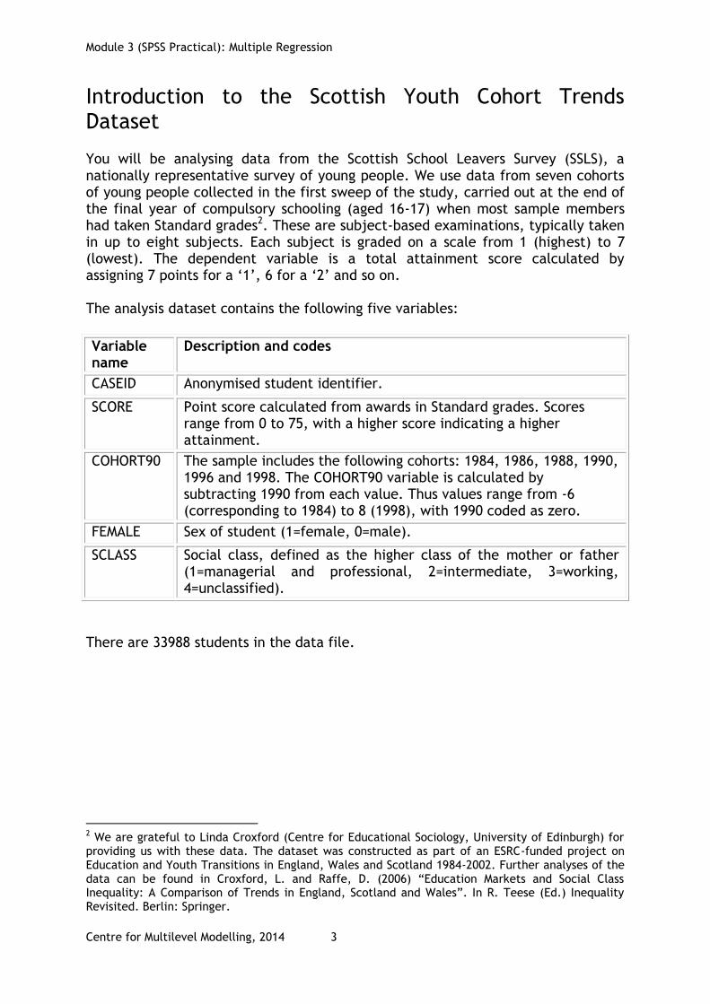
Introduction to the Scottish Youth Cohort Trends Dataset You will be analysing data from the Scottish School Leavers Survey (SSLS), a nationally representative survey of young people. We use data from seven cohorts of young people collected in the first sweep of the study, carried out at the end of the final year of compulsory schooling (aged 16-17) when most sample members had taken Standard grades2. These are subject-based examinations, typically taken in up to eight subjects. Each subject is graded on a scale from 1 (highest) to 7 (lowest). The dependent variable is a total attainment score calculated by assigning 7 points for a ‘1’, 6 for a ‘2’ and so on. The analysis dataset contains the following five variables:

Variable name

Description and codes

CASEID Anonymised student identifier.

SCORE Point score calculated from awards in Standard grades. Scores range from 0 to 75, with a higher score indicating a higher attainment.

COHORT90 The sample includes the following cohorts: 1984, 1986, 1988, 1990, 1996 and 1998. The COHORT90 variable is calculated by subtracting 1990 from each value. Thus values range from -6 (corresponding to 1984) to 8 (1998), with 1990 coded as zero.

FEMALE Sex of student (1=female, 0=male).

SCLASS Social class, defined as the higher class of the mother or father (1=managerial and professional, 2=intermediate, 3=working, 4=unclassified).

There are 33988 students in the data file.

2 We are grateful to Linda Croxford (Centre for Educational Sociology, University of Edinburgh) for providing us with these data. The dataset was constructed as part of an ESRC-funded project on Education and Youth Transitions in England, Wales and Scotland 1984-2002. Further analyses of the data can be found in Croxford, L. and Raffe, D. (2006) “Education Markets and Social Class Inequality: A Comparison of Trends in England, Scotland and Wales”. In R. Teese (Ed.) Inequality Revisited. Berlin: Springer.

Module 3 (SPSS Practical): Multiple Regression

Centre for Multilevel Modelling, 2014 4

P3.1 Regression with a Single Continuous Explanatory Variable

P3.1 Regression with a Single Continuous Explanatory Variable

We will begin by looking at the relationship between attainment (SCORE) and cohort (COHORT90). Has attainment changed over time and, if so, is the trend linear?

P3.1.1 Examining the data To access the data files associated with this tutorial, you must have an account with LEMMA. To open the first data file, From within the LEMMA Learning Environment

Go to Module 3: Multiple regression, and scroll down to SPSS Datafiles

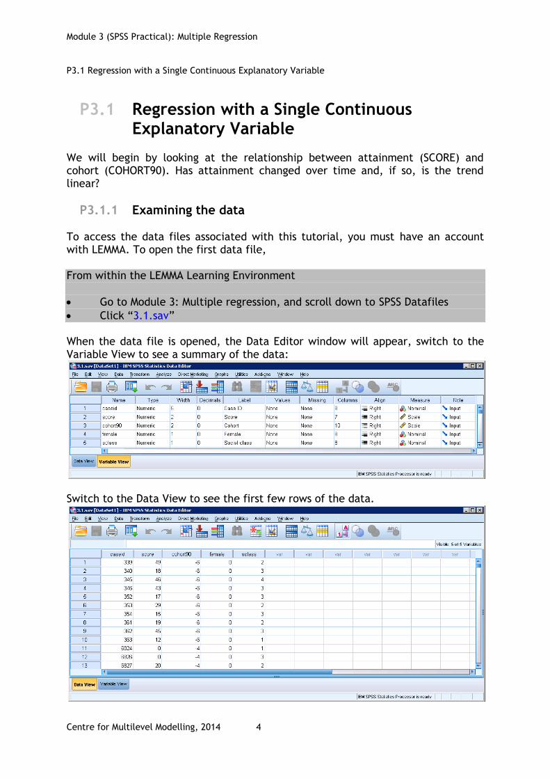
Click “3.1.sav” When the data file is opened, the Data Editor window will appear, switch to the Variable View to see a summary of the data:

Switch to the Data View to see the first few rows of the data.

Module 3 (SPSS Practical): Multiple Regression

Centre for Multilevel Modelling, 2014 5

SPSS can be operated either via its point-and-click environment or through scripting commands. Although the menus can be useful when doing exploratory work it is good practice to work with commands and generate syntax files to allow replication. Because of these we will be using script commands for this exercise. The menu options can be useful when learning the syntax, so we also provide alternative instructions for these where they exist. SPSS can display the command that corresponds to choices made in the menus. To check that this is enabled open Edit>Options>Viewer and check "Display commands in the log" is ticked. SPSS can also automatically generate the syntax corresponding to the current dialog box, which can then be edited before being run. This is done using the “Paste” button at the bottom of the dialog box. To run commands interactively in SPSS:

File>New>Syntax

Enter the required commands into the syntax window

Highlight the command to run

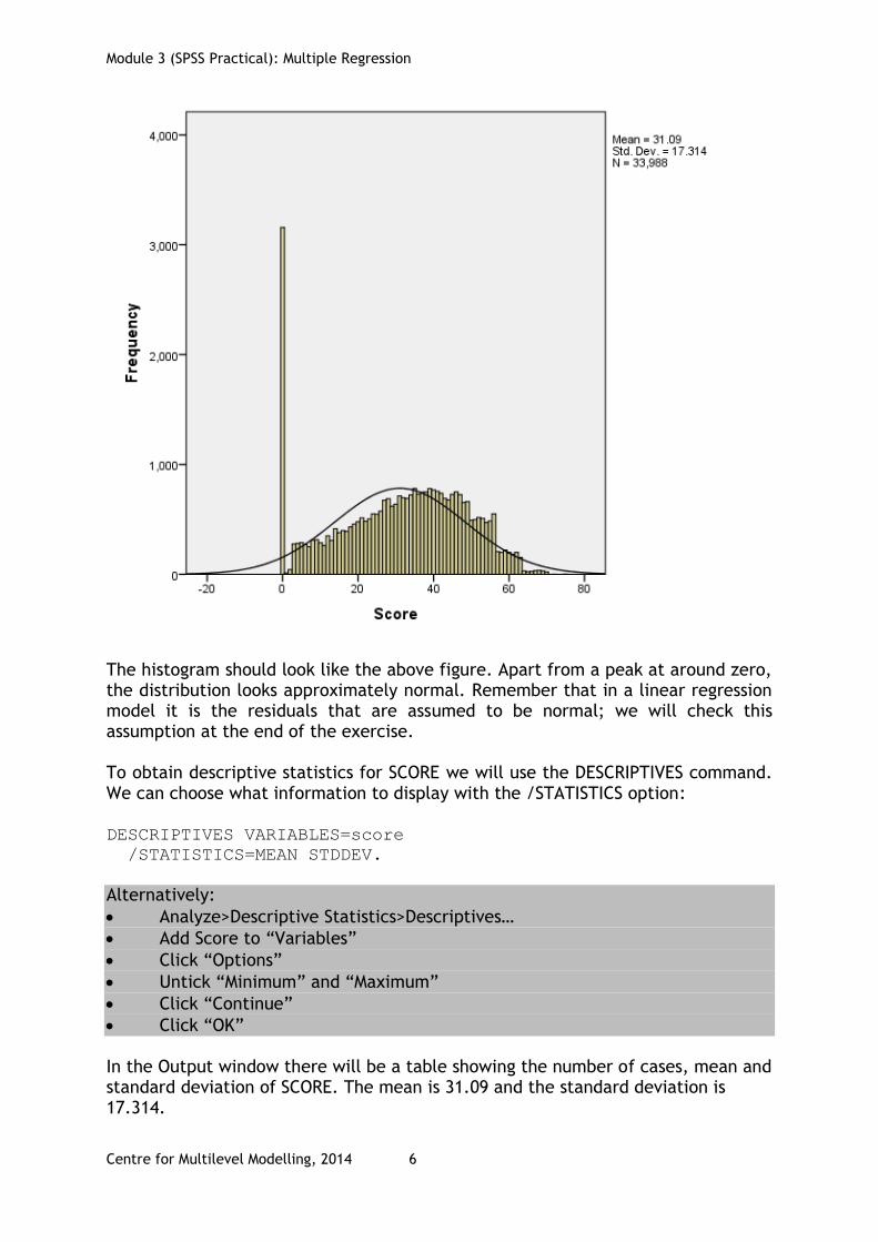
Click “Run selection” (indicated by a green ► button in the toolbar) Having viewed the data we will examine SCORE and COHORT90, the variables to be considered in our first regression analysis. Distribution of SCORE We will begin by obtaining a histogram and descriptive statistics for the dependent variable, SCORE. To obtain a histogram we will use the GRAPH command with the /HISTOGRAM option. Adding NORMAL in brackets will cause a normal curve to also be plot on the graph: GRAPH

/HISTOGRAM(NORMAL)=score.

Alternatively:

Graphs>Legacy Dialogs>Histogram

Add score to “Variable”

Tick “Display normal curve”

Click “Paste”

Compare the generated syntax with that above

Highlight the syntax

Click the green ► button

Module 3 (SPSS Practical): Multiple Regression

Centre for Multilevel Modelling, 2014 6

The histogram should look like the above figure. Apart from a peak at around zero, the distribution looks approximately normal. Remember that in a linear regression model it is the residuals that are assumed to be normal; we will check this assumption at the end of the exercise. To obtain descriptive statistics for SCORE we will use the DESCRIPTIVES command. We can choose what information to display with the /STATISTICS option: DESCRIPTIVES VARIABLES=score

/STATISTICS=MEAN STDDEV.

Alternatively:

Analyze>Descriptive Statistics>Descriptives…

Add Score to “Variables”

Click “Options”

Untick “Minimum” and “Maximum”

Click “Continue”

Click “OK” In the Output window there will be a table showing the number of cases, mean and standard deviation of SCORE. The mean is 31.09 and the standard deviation is 17.314.

This document is only the first few pages of the full version. To see the complete document please go to learning materials and register: http://www.cmm.bris.ac.uk/lemma The course is completely free. We ask for a few details about yourself for our research purposes only. We will not give any details to any other organisation unless it is with your express permission.