mohammad h. kurdi*, tony l. schmitz and raphael t. haftka

Int. J. Materials and Product Technology, Vol. x, No. x, xxxx 1

Copyright © 200x Inderscience Enterprises Ltd.

Milling optimisation of removal rate and accuracy with uncertainty: part 1: parameter selection

Mohammad H. Kurdi*, Tony L. Schmitz and Raphael T. Haftka Mechanical and Aerospace Engineering Department, University of Florida, Gainesville, FL 32611 Fax: +937-656-4945 E-mail: [email protected] E-mail: [email protected] E-mail: [email protected] *Corresponding author

Brian P. Mann Mechanical and Aerospace Engineering Department, University of Missouri, Columbia, MO 65211, USA E-mail: [email protected]

Abstract: Successful implementation of milling requires the selection of appropriate operating parameters. In this paper a semi-analytical modeling approach and multi-objective optimisation are used to select optimum spindle speed and axial depth. The trade-off curve of removal rate and surface location error is calculated. Some degree of robustness is achieved by calculating the surface location error as a moving average over an interval of spindle speeds. The stability boundary and a selected design are compared to experimental results. The results illustrate the need to be concerned with the robustness of the optimal designs. This is addressed in Part 2 of the paper.

Keywords: milling optimisation; multi-objective; sensitivity; Pareto; uncertainty; correlation; stability.

Reference to this paper should be made as follows: Kurdi, M.H., Schmitz, T.L., Haftka, R.T. and Mann, B.P. (xxxx) ‘Milling optimisation of removal rate and accuracy with uncertainty: part 1: parameter selection’, Int. J. Materials and Product Technology, Vol. x, No. x, pp.xxx–xxx.

Biographical notes: Mohammad H. Kurdi is a National Research Council Postdoctoral Associate at the Air Force Research Laboratory. Mohammad completed his BSc at University of Jordan and his PhD at University of Florida in 2005. His research interests include multi-objective optimisation, design under uncertainty and advanced computational methods. Current projects are in uncertainty quantification of flutter boundaries in aircraft structures.

Tony L. Schmitz is an Assistant Professor in the Department of Mechanical and Aerospace Engineering at the University of Florida, where he is the Director of the Machine Tool Research Center. His primary interests are in the fields of manufacturing metrology and process dynamics with a current projects in high-speed machining and displacement measuring interferometry. Recent professional recognitions include the National Science Foundation

2 M.H. Kurdi et al.

CAREER award, Office of Naval Research Young Investigator award, and the Society of Manufacturing Engineers Outstanding Young Manufacturing Engineer award. He received his PhD from the University of Florida in 1999.

Raphael (Rafi) T. Haftka completed his Undergraduate Education at Technion Israel and his PhD at UC San Diego. He has taught at Technion, Illinois Institute of Technology, and Virginia Tech before coming to the University of Florida in 1995 where he is a Distinguished Professor. His research is in the areas of structural and multidisciplinary optimisation and DESIGN under Uncertainty, which gives him the opportunity and pleasure to collaborate with many colleagues. He has co-authored papers with more than 100 peers in 13 countries. He has authored two textbooks and hundreds of papers, and his work was cited by more than 2500 journal papers.

Brian P. Mann is an Assistant Professor in the Department of Mechanical and Aerospace Engineering at the University of Missouri – Columbia. He received his DSc Degree in 2003 from Washington University St. Louis. Past honours include being awarded the National Defense Science and Engineering Graduate Fellowship and a CAREER Award from the National Science Foundation. His general research interests are in vibration phenomena, non-linear dynamics, and in the influence of time delays on stability.

1 Introduction

Intense competition in manufacturing demands cost-effective manufacturing processes that provide acceptable dimensional accuracy. Milling often satisfies these requirements provided appropriate operating parameters are selected. However, the selection of these preferred operating parameters is not trivial. Barriers to the full realisation of potential productivity gains include:

• the requirement for multiple tool point dynamic measurements

• sensitivity of part quality to small changes in process variables

• the difficulty in concurrently considering stability, accuracy, and surface finish in an analytical (or semi-analytical) framework.

Therefore, balancing the multiple requirements, including high material removal rate, MRR, minimum surface location error (deviation of the actual cut surface from the commanded one resulting from the process dynamics), SLE, sufficient tool life, chatter avoidance, and adequate surface finish, to arrive at an optimum solution is difficult without the aid of optimisation techniques.

Prior research in milling (particularly high-speed milling) optimisation has considered a single objective. For example, Kim et al. (2002) focused on optimising cutting speed to improve machining accuracy in high-speed ball end milling by accounting for the effective tool diameter during cutting. Juan et al. (2003) applied the concept of adaptive learning (polynomial network) to construct a machining model that gathered material removal, cost and time components of high-speed milling operations and then used simulated annealing optimisation to select optimum cutting parameters to minimise production cost for rough high-speed machining operations. In this study, a mathematical

Milling optimisation of removal rate and accuracy with uncertainty 3

model is used to analyse the process dynamics directly with regard to surface accuracy and stability with axial depth of cut and spindle speed as design variables. Other considerations such as tool wear and inclusion of more process parameters may be included in the future.

Previous research in machining process optimisation has explored various objective functions. Three main objectives have been recognised:

• maximum production rate or minimum cycle time (Deshayes et al., 2005)

• minimum cost (Ermer, 1971; Hitomi, 1989; Shalaby and Riad, 1988; Hati and Rao, 1976)

• maximum profit (Wu and Ermer, 1966; Boothroyd and Rusek, 1976).

Agapiou (1992) considered a combined criterion based on a weighted sum of these. We apply multi-objective optimisation, which addresses the issue of competing objectives using concepts developed by Pareto (Schwier, 1971), the French-Italian economist who established an optimality concept in the field of economics for multiple objectives. A Pareto front (Kalyanmoy, 2001) is generated that allows designers to tradeoff one objective against others. This has the advantage of giving the designer the opportunity to tradeoff objectives directly, in contrast to optimising a weighted sum of the two objectives, where the weights selected by the designer may not correspond to a desirable tradeoff. Additionally, the Pareto front enables the designer to view the set of possible optimum designs and select his or her preference depending on the particular product objective. However, generating a Pareto front is typically much more expensive than optimising a single objective. Due to the computational intensity of the Pareto front calculation, an efficient analysis method should be used. The semi-analytical Time Finite Element Analysis (TFEA) (Mann, 2003; Halley, 1999; Mann et al., 2004) approach is used here to obtain rapid process performance calculations of SLE and stability in a single step. The computational efficiency of TFEA compared to conventional time-domain simulation methods makes it an attractive candidate for use in the optimisation algorithm. Additionally, TFEA provides a clear and distinct definition of stability boundaries (i.e., characteristic multipliers of the milling equation with an absolute value greater than one identify unstable conditions, see Section 2.2).

In this paper we seek to develop a framework for pre-process selection of milling parameters. In Part 1, we calculate the Pareto front of SLE and MRR considering process stability. Additionally, we account for the regions of high SLE sensitivity to small changes in parameters using a moving average SLE objective. An experimental case study is presented which evaluates the robustness of designs to SLE sensitivity and stability. Although the study verifies the optimisation formulation, it also highlights the need to consider process parameter uncertainties due to disagreement between SLE prediction and experiment. In Part 2 of the paper we explore the influence of input uncertainties on prediction distributions. Sampling methods are used to propagate the input parameter uncertainties through the TFEA analysis. We identify the importance of considering correlations between parameters to mimic actual physical variations and show that when correlation is included, the propagated uncertainty better represents experimental results.

4 M.H. Kurdi et al.

The main objectives of the paper are summarised as: • develop an optimisation method that accounts for objective sensitivity to small

changes in a design variable • calculate the Pareto front of SLE and MRR under stability constraints • verify the robustness of the optimisation algorithm experimentally and evaluate

uncertainty.

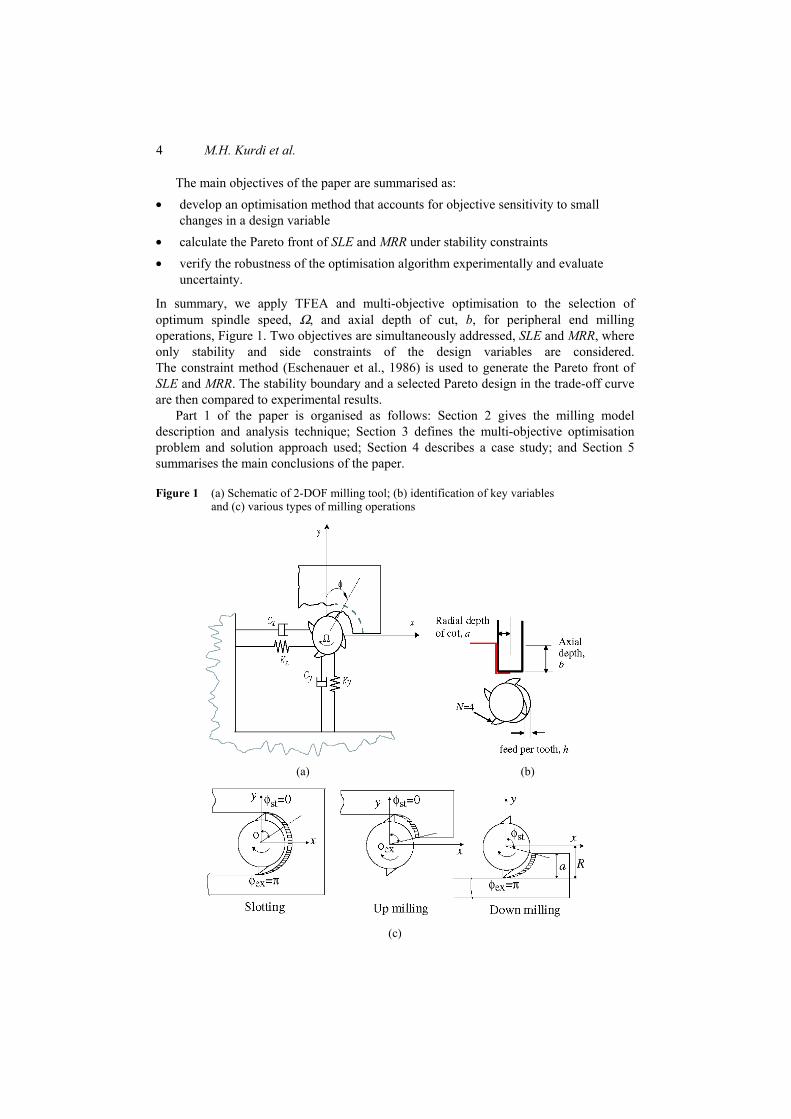
In summary, we apply TFEA and multi-objective optimisation to the selection of optimum spindle speed, Ω, and axial depth of cut, b, for peripheral end milling operations, Figure 1. Two objectives are simultaneously addressed, SLE and MRR, where only stability and side constraints of the design variables are considered. The constraint method (Eschenauer et al., 1986) is used to generate the Pareto front of SLE and MRR. The stability boundary and a selected Pareto design in the trade-off curve are then compared to experimental results.

Part 1 of the paper is organised as follows: Section 2 gives the milling model description and analysis technique; Section 3 defines the multi-objective optimisation problem and solution approach used; Section 4 describes a case study; and Section 5 summarises the main conclusions of the paper.

Figure 1 (a) Schematic of 2-DOF milling tool; (b) identification of key variables and (c) various types of milling operations

(a) (b)

(c)


2 Milling problem

2.1 Milling model

In this paper we consider a two Degree-of-Freedom (2-DOF) analysis (see Figure 1(a)) of the milling operation for optimisation. However, the semi-analytical approach described here is also applicable to milling processes with multiple DOF (Mann et al., 2005). With the assumption of either a compliant tool or structure, a summation of forces gives the following equation of motion in orthogonal physical coordinates:

0 0 0 ( )( ) ( ) ( ),

0 0 0 ( )( ) ( ) ( )x X x x

y y y y

M C K F tx t x t x tM C K F ty t y t y t

+ + =

(1)

where Mx, Cx, Kx and My, Cy, Ky are the modal mass, viscous damping, and stiffness terms and Fx and Fy are the cutting forces in the x and y-directions, respectively. A compact form of the milling process can be found by considering the chip thickness variation and forces on each tooth (a detailed derivation is provided in references (Mann, 2003; Halley, 1999; Mann et al., 2004, 2005):

0( ) ( ) ( ) ( ) ( ( ) ( )) ( ) ,X t X t X t t b X t X t f t bτ+ + = − − +cM C K K (2)

where [ ]( ) ( ) ( ) TX t x t y t= is the two-element position vector; M, C and K are the 2 × 2 modal mass, damping, and stiffness matrices, respectively; Kc is a 2 × 2 matrix representing the component of cutting forces which depend on the position vector and

0 ( )f t is the 2 × 1 vector that represents the component of the cutting forces that are independent of the position vector; b is the axial depth of cut; τ = 60/(NΩ) is the tooth passing period; N is the number of cutting teeth on the cutting tool; Ω is the spindle speed in rev/min (rpm). As shown in equation (2), the milling model depends on modal parameters of the tool or workpiece and the cutting force coefficients. In Part 2 of this paper we describe the experimental procedure used to estimate these parameters.

2.2 Analysis method

The dynamic behaviour of the milling process, governed by equation (2), can be determined using numerical time-domain simulation (Smith and Tlusty, 1991) or the semi-analytical TFEA. As noted previously, TFEA is numerically more efficient. Using this method, a dynamic map (matrices generated using weighted residual projection of the time dimension in equation (2)) is generated that relates the vibration while the tool is in the cut to free vibration out of the cut. Stability of the milling process can be determined using the characteristic multipliers of the dynamic map; SLE is found from the fixed points or steady-state solution of the dynamic map. For a more detailed description of the method the interested reader may refer to Mann et al. (2005).

The use of TFEA in an optimisation algorithm requires ascertaining its convergence characteristics in the entire design domain. The convergence of TFEA depends on the number of elements and cutting parameters, including spindle speed and radial depth of cut. Both |SLE| and the characteristic multipliers of the dynamic map can be used to check for convergence. The stability boundary is determined using the maximum magnitude of the characteristic multipliers:

6 M.H. Kurdi et al.

max max ,kkλ λ= (3)

where λk denotes the kth characteristic multiplier of the dynamic map. A typical convergence test is to observe the change in the estimated value (λmax or |SLE|) as the number of elements (mesh refinement) or interpolating polynomials order (Garg et al., 2007) is increased. In Figure 2, the dependence of λmax on the number of elements for three spindle speeds is shown for a randomly selected cutting condition of 5% radial immersion (i.e., the percentage of radial depth of cut to tool diameter) and 18 mm axial depth. As shown in panel (b), false convergence for a small number of elements (≤3) can occur. However, increasing the number of elements (>3) shows poor convergence for both lower speeds. A convergent solution is reached for the 1000 rpm spindle speed for fewer elements (E = 11) than for the 500 rpm case (E = 17). This is due to the fact that, as the spindle speed decreases, the time in the cut increases, which requires a higher number of elements to achieve convergence. Because the optimisation algorithm will pick milling parameters anywhere within the design space, it is necessary to choose a sufficiently high number of elements to ensure convergence over the full test range. However, a penalty in computational time is incurred for more elements. Since the greatest potential for high MRR is in the higher spindle speed range, a minimum spindle speed of 5000 rpm is used here. This ensures that a typical number of elements (E = 10 is used in the following analyses) is efficient and adequate (see Figure 2).

2.2.1 Stability boundary

In order to find the axial depth stability limit, blim, at the corresponding cutting conditions, the bi-section method is used to solve for the axial depth at which λmax = 1 (stability limit). An absolute error is used as a criterion for convergence:

1 ,i i

i

b bb

ε−−≤ (4)

where ε is the convergence tolerance and bi is the axial depth corresponding to λmax = 1 at iteration i. The value of ε is based on the numerical accuracy required in the calculation of blim. A value of ε = 0.001 is usually acceptable.

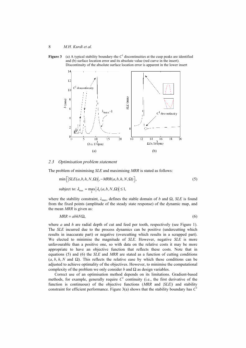
A typical example for the calculation of the stability limit, blim, is shown in Figure 3(a) where the variation of blim vs. spindle speed shows lobe peaks where C1 (slope) discontinuity of the stability boundary is observed. The discontinuity happens when two characteristicmultipliers change places in terms of having the largest magnitude. Accounting for this discontinuity is important in the implementation of the optimisation search method.


Figure 2 Convergence plots of the stability constraint showing the effect of spindle speed on convergence for 5% radial immersion and an 18 mm axial depth: (a) 500, 1000, 5000 rpm compared for full range of number of elements; (b) false convergence of 500, 1000 rpm speeds for number of elements ≤3; (c) convergent solution for all spindle speeds and (d) convergent solution for 1000, 5000 rpm. It is seen that convergence at lower speeds requires more elements

(a)

(b)

(c)

(d)

8 M.H. Kurdi et al.

Figure 3 (a) A typical stability boundary-the C1 discontinuities at the cusp peaks are identified and (b) surface location error and its absolute value (red curve in the insert). Discontinuity of the absolute surface location error is apparent in the lower insert

(a) (b)

2.3 Optimisation problem statement

The problem of minimising SLE and maximising MRR is stated as follows:

min ( , , , , ) , ( , , , , ) ,SLE a b h N MRR a b h N Ω − Ω (5)

maxsubject to: max ( , , , ) 1,kka b Nλ λ= Ω ≤

where the stability constraint, λmax, defines the stable domain of b and Ω, SLE is found from the fixed points (amplitude of the steady state response) of the dynamic map, and the mean MRR is given as:

,MRR abhN= Ω (6)

where a and h are radial depth of cut and feed per tooth, respectively (see Figure 1). The SLE incurred due to the process dynamics can be positive (undercutting which results in inaccurate part) or negative (overcutting which results in a scrapped part). We elected to minimise the magnitude of SLE. However, negative SLE is more unfavourable than a positive one, so with data on the relative costs it may be more appropriate to have an objective function that reflects these costs. Note that in equations (5) and (6) the SLE and MRR are stated as a function of cutting conditions (a, b, h, N and Ω). This reflects the relative ease by which these conditions can be adjusted to achieve optimality of the objectives. However, to minimise the computational complexity of the problem we only consider b and Ω as design variables.

Correct use of an optimisation method depends on its limitations. Gradient-based methods, for example, generally require C1 continuity (i.e., the first derivative of the function is continuous) of the objective functions (MRR and |SLE|) and stability constraint for efficient performance. Figure 3(a) shows that the stability boundary has C1


discontinuities near lobe peaks. The reader may note some irregularity in the bottom part of the stability boundary. This is mainly due to the analysis method (TFEA), which considers the interrupted nature of the cutting process. This can lead to two types of instability: Hopf and flip bifurcations. These irregularities are due to flip bifurcation and become more pronounced at very small radial depths of cut. Figure 3(b) depicts the variation of SLE and |SLE| as a function of spindle speed for a typical set of cutting parameters. Although SLE is C1 continuous, the absolute value is discontinuous where SLE switches sign. C1 discontinuity inhibits rapid convergence of gradient-based optimisation algorithms. To overcome this difficulty we use multiple initial guesses procedure to enable convergence of the optimisation method to local optima (see Section 3.2).

3 Multi-objective optimisation formulation

In this section a discussion of the concepts of single and multi-objective optimisation is briefly provided, the interested reader may refer to the book by Miettinen (1999) for a more elaborate discussion. The multi-objective problem is formulated using the constraint method and then a robust formulation is provided to account for the sensitivity of the |SLE| objective to spindle speed.

3.1 Single and multi-objective optimisation

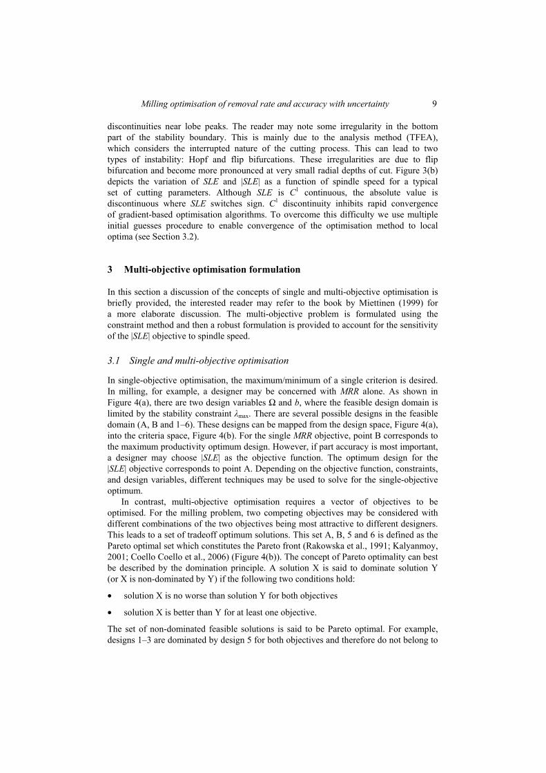
In single-objective optimisation, the maximum/minimum of a single criterion is desired. In milling, for example, a designer may be concerned with MRR alone. As shown in Figure 4(a), there are two design variables Ω and b, where the feasible design domain is limited by the stability constraint λmax. There are several possible designs in the feasible domain (A, B and 1–6). These designs can be mapped from the design space, Figure 4(a), into the criteria space, Figure 4(b). For the single MRR objective, point B corresponds to the maximum productivity optimum design. However, if part accuracy is most important, a designer may choose |SLE| as the objective function. The optimum design for the |SLE| objective corresponds to point A. Depending on the objective function, constraints, and design variables, different techniques may be used to solve for the single-objective optimum.

In contrast, multi-objective optimisation requires a vector of objectives to be optimised. For the milling problem, two competing objectives may be considered with different combinations of the two objectives being most attractive to different designers. This leads to a set of tradeoff optimum solutions. This set A, B, 5 and 6 is defined as the Pareto optimal set which constitutes the Pareto front (Rakowska et al., 1991; Kalyanmoy, 2001; Coello Coello et al., 2006) (Figure 4(b)). The concept of Pareto optimality can best be described by the domination principle. A solution X is said to dominate solution Y (or X is non-dominated by Y) if the following two conditions hold:

• solution X is no worse than solution Y for both objectives

• solution X is better than Y for at least one objective.

The set of non-dominated feasible solutions is said to be Pareto optimal. For example, designs 1–3 are dominated by design 5 for both objectives and therefore do not belong to

10 M.H. Kurdi et al.

the Pareto optimal set. Although design 4 dominates design 5, it is dominated by design 6 which excludes it from the Pareto set. Designs which belong to the Pareto front are candidate designs that trade off one objective against the other. Depending on the decision maker’s preferences, a single solution can be chosen from that set.

Figure 4 (a) Design variables b and Ω, and constraint λmax in the design space and (b) corresponding Pareto front in the criterion space

(a)

(b)

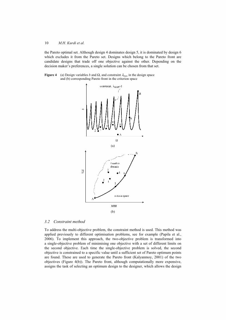
3.2 Constraint method

To address the multi-objective problem, the constraint method is used. This method was applied previously to different optimisation problems, see for example (Papila et al., 2006). To implement this approach, the two-objective problem is transformed into a single-objective problem of minimising one objective with a set of different limits on the second objective. Each time the single-objective problem is solved, the second objective is constrained to a specific value until a sufficient set of Pareto optimum points are found. These are used to generate the Pareto front (Kalyanmoy, 2001) of the two objectives (Figure 4(b)). The Pareto front, although computationally more expensive, assigns the task of selecting an optimum design to the designer, which allows the design


to evolve according to product requirements. In the case that |SLE| is chosen as the objective function to be minimised, equation (5) is transformed to:

max

min ( , )subject to: ( , ) , for 1

( , ) max ( , ) 1,i

kk

SLE bMRR b e i k

b bλ λ

Ω− Ω ≤ =

Ω = Ω ≤… (7)

for a series of k selected limits (ei) on MRR, where the axial depth (b) and spindle speed (Ω) are the design variables. The boundary of the limits ei is based on the designer’s preferences and stability constraint limitation. For example, points A and B in Figure 4(b) may be set as the minimum MRR tolerated by the designer and the maximum MRR possible in the design domain, respectively.

The Sequential Quadratic Programming method (SQP) is used to find the Pareto front using the formulation in equation (7). The SQP method is a local search method that is dependent on C1 continuity of the objective function and constraints. However, the use of multiple initial guesses circumvents this weakness. The fmincon function in the Matlab optimisation toolbox is used to implement the method. To obtain a global optimum, initial guesses are made at selected spindle speeds (we have used 1000 rpm intervals in the spindle speed range) along each MRR constraint limit. A set of designs are obtained from these initial guesses. The minimum of these designs is nominated as a global optimum. However, since designs found by fmincon are not necessarily optimal designs, the number of initial guesses along the MRR constraint is increased and the optimisation simulation is again executed to check the validity of that global optimum.

A numerical example was completed; the down milling cutting conditions are provided in Table 1. Modal parameters for a two flute, 19.05 mm diameter, d, 12° helix angle tool with one mode in the x- and y-directions and nominal values of the tangential, Kt, and normal, Kn, cutting force coefficients and edge coefficients Kte and Kne, are also given (the coefficients are used to compute the cutting forces in equation (1)). Numerical results for four selected limits on MRR are shown in Figure 5.

Table 1 Cutting conditions, cutting force coefficients and modal parameters for numerical example shown in Figure 5

M (kg) C (N.s/m) K (N/m)

0.056 0 3.94 0 1.52 × 106 0 0 0.061 0 3.86 0 1.67 × 106

d (mm) h (mm) a (mm) N 19.05 0.18 0.76 2

Kt (N/m2) Kn (N/m2) Kte (N/m) Kne (N/m) 550 × 106 200 × 106 0 0


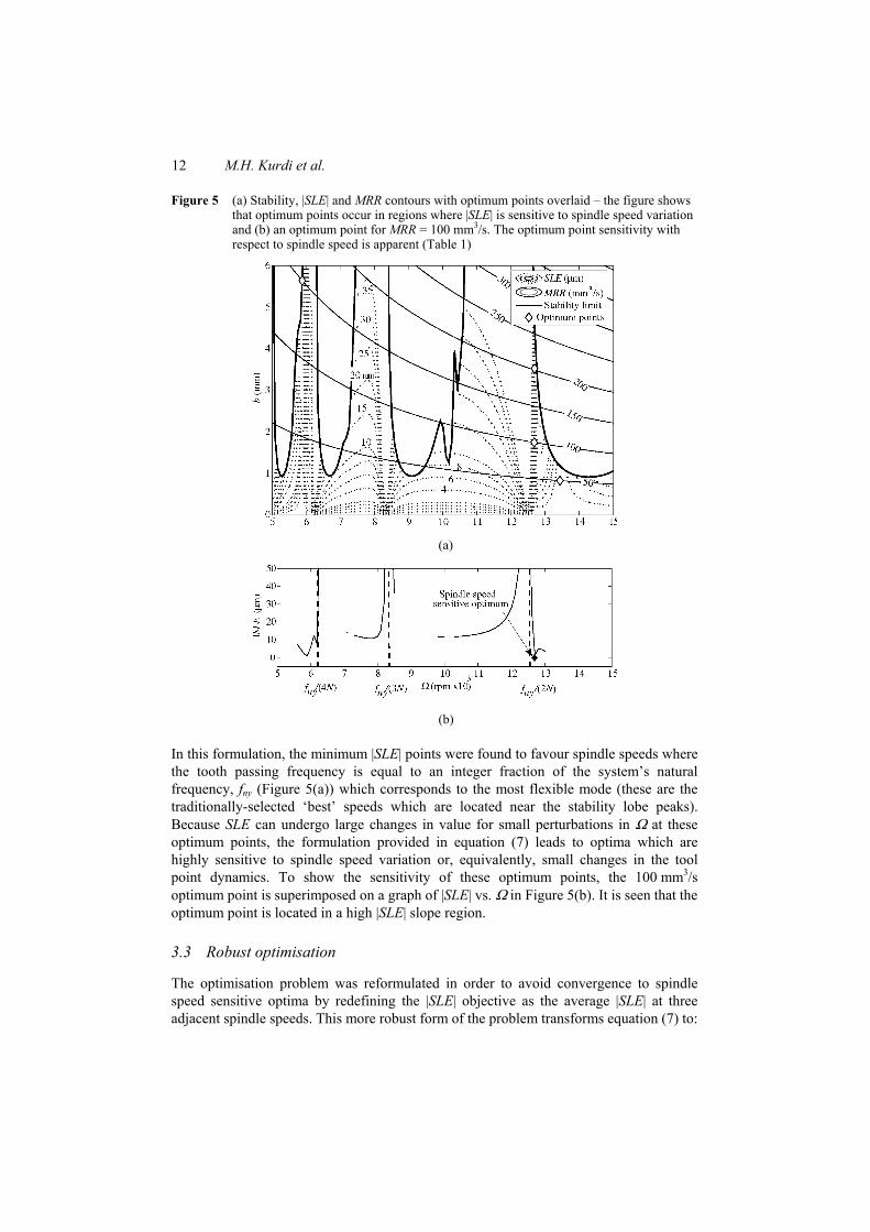
Figure 5 (a) Stability, |SLE| and MRR contours with optimum points overlaid – the figure shows that optimum points occur in regions where |SLE| is sensitive to spindle speed variation and (b) an optimum point for MRR = 100 mm3/s. The optimum point sensitivity with respect to spindle speed is apparent (Table 1)

(a)

(b)

In this formulation, the minimum |SLE| points were found to favour spindle speeds where the tooth passing frequency is equal to an integer fraction of the system’s natural frequency, fny (Figure 5(a)) which corresponds to the most flexible mode (these are the traditionally-selected ‘best’ speeds which are located near the stability lobe peaks). Because SLE can undergo large changes in value for small perturbations in Ω at these optimum points, the formulation provided in equation (7) leads to optima which are highly sensitive to spindle speed variation or, equivalently, small changes in the tool point dynamics. To show the sensitivity of these optimum points, the 100 mm3/s optimum point is superimposed on a graph of |SLE| vs. Ω in Figure 5(b). It is seen that the optimum point is located in a high |SLE| slope region.

3.3 Robust optimisation

The optimisation problem was reformulated in order to avoid convergence to spindle speed sensitive optima by redefining the |SLE| objective as the average |SLE| at three adjacent spindle speeds. This more robust form of the problem transforms equation (7) to:


max max max

( , ) ( , ) ( , )min

3

subject to: ( , ) , for 1 ( , ) ( , ) ( , ) 1,

i

SLE b SLE b SLE b

MRR b e i kb b b

δ δ

λ δ λ λ δ

Ω + + Ω + Ω −

− Ω ≤ =Ω − Ω Ω + ≤

…∩ ∩

(8)

for a series of k selected limits (ei) on MRR. The spindle speeds include the nominal Ω plus two perturbations Ω + δ and Ω – δ. The additional evaluations of SLE and stability constraint triples the computation time of the optimisation. The perturbation, δ, is selected by the designer based on the confidence in the natural frequency of the tool/workpiece combination (a 50 rpm perturbation was used in our analyses).

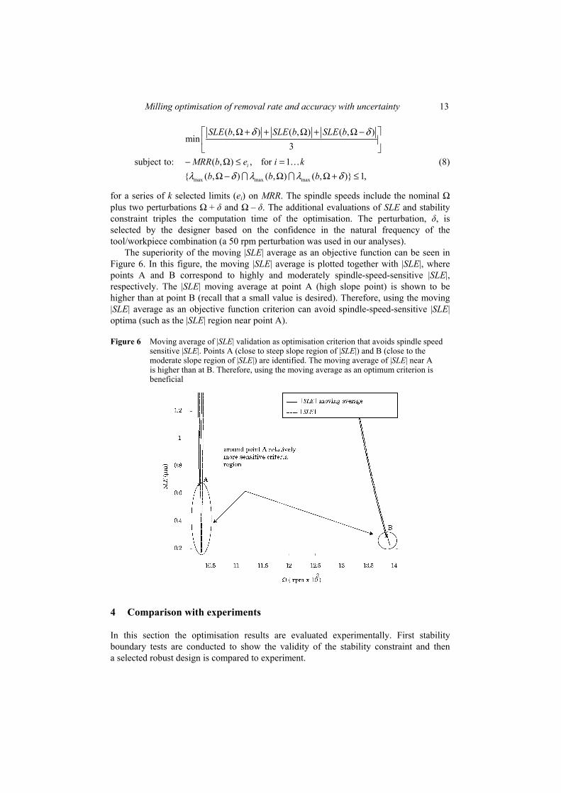
The superiority of the moving |SLE| average as an objective function can be seen in Figure 6. In this figure, the moving |SLE| average is plotted together with |SLE|, where points A and B correspond to highly and moderately spindle-speed-sensitive |SLE|, respectively. The |SLE| moving average at point A (high slope point) is shown to be higher than at point B (recall that a small value is desired). Therefore, using the moving |SLE| average as an objective function criterion can avoid spindle-speed-sensitive |SLE| optima (such as the |SLE| region near point A).

Figure 6 Moving average of |SLE| validation as optimisation criterion that avoids spindle speed sensitive |SLE|. Points A (close to steep slope region of |SLE|) and B (close to the moderate slope region of |SLE|) are identified. The moving average of |SLE| near A is higher than at B. Therefore, using the moving average as an optimum criterion is beneficial

4 Comparison with experiments

In this section the optimisation results are evaluated experimentally. First stability boundary tests are conducted to show the validity of the stability constraint and then a selected robust design is compared to experiment.


4.1 Stability boundary tests

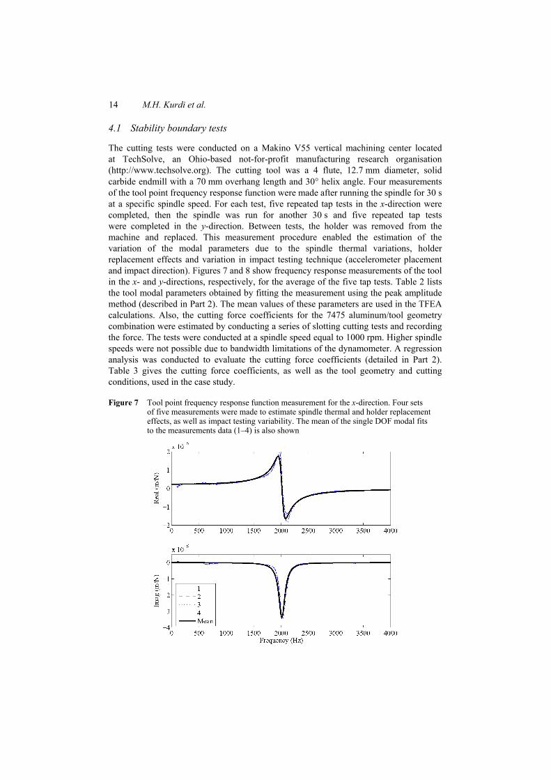
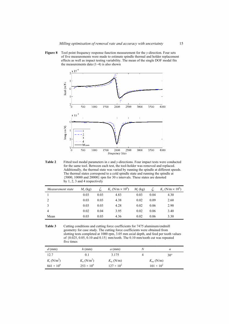
The cutting tests were conducted on a Makino V55 vertical machining center located at TechSolve, an Ohio-based not-for-profit manufacturing research organisation (http://www.techsolve.org). The cutting tool was a 4 flute, 12.7 mm diameter, solid carbide endmill with a 70 mm overhang length and 30° helix angle. Four measurements of the tool point frequency response function were made after running the spindle for 30 s at a specific spindle speed. For each test, five repeated tap tests in the x-direction were completed, then the spindle was run for another 30 s and five repeated tap tests were completed in the y-direction. Between tests, the holder was removed from the machine and replaced. This measurement procedure enabled the estimation of the variation of the modal parameters due to the spindle thermal variations, holder replacement effects and variation in impact testing technique (accelerometer placement and impact direction). Figures 7 and 8 show frequency response measurements of the tool in the x- and y-directions, respectively, for the average of the five tap tests. Table 2 lists the tool modal parameters obtained by fitting the measurement using the peak amplitude method (described in Part 2). The mean values of these parameters are used in the TFEA calculations. Also, the cutting force coefficients for the 7475 aluminum/tool geometry combination were estimated by conducting a series of slotting cutting tests and recording the force. The tests were conducted at a spindle speed equal to 1000 rpm. Higher spindle speeds were not possible due to bandwidth limitations of the dynamometer. A regression analysis was conducted to evaluate the cutting force coefficients (detailed in Part 2). Table 3 gives the cutting force coefficients, as well as the tool geometry and cutting conditions, used in the case study.

Figure 7 Tool point frequency response function measurement for the x-direction. Four sets of five measurements were made to estimate spindle thermal and holder replacement effects, as well as impact testing variability. The mean of the single DOF modal fits to the measurements data (1–4) is also shown


Figure 8 Tool point frequency response function measurement for the y-direction. Four sets of five measurements were made to estimate spindle thermal and holder replacement effects as well as impact testing variability. The mean of the single DOF modal fits the measurements data (1–4) is also shown

Table 2 Fitted tool modal parameters in x and y-directions. Four impact tests were conducted for the same tool. Between each test, the tool-holder was removed and replaced. Additionally, the thermal state was varied by running the spindle at different speeds. The thermal states correspond to a cold spindle state and running the spindle at 5000, 10000 and 20000 rpm for 30 s intervals. These states are denoted by 1, 2, 3 and 4 respectively

Measurement state Mx (kg) ζx Kx (N/m × 106) My (kg) ζy Ky (N/m × 106) 1 0.03 0.03 4.83 0.03 0.04 4.30 2 0.03 0.03 4.38 0.02 0.09 2.60 3 0.03 0.03 4.28 0.02 0.06 2.90 4 0.02 0.04 3.95 0.02 0.06 3.40 Mean 0.03 0.03 4.36 0.02 0.06 3.30

Table 3 Cutting conditions and cutting force coefficients for 7475 aluminum/endmill geometry for case study. The cutting force coefficients were obtained from slotting tests completed at 1000 rpm, 3.05 mm axial depth, and feed per tooth values of 0.025, 0.05, 0.10 and 0.15 mm/tooth. The 0.10 mm/tooth cut was repeated five times

d (mm) h (mm) a (mm) N α

12.7 0.1 3.175 4 30° Kt (N/m2) Kn (N/m2) Kte (N/m) Kne (N/m) 841 × 106 253 × 106 127 × 102 101 × 102


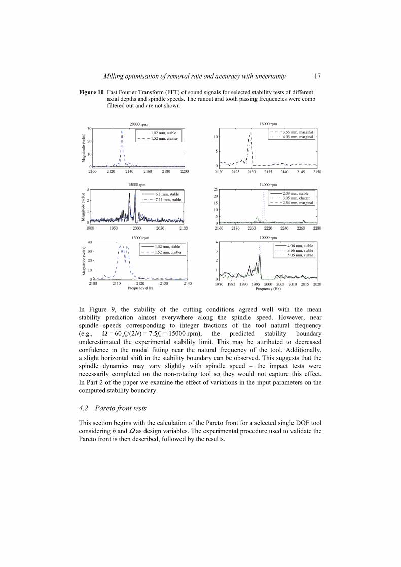
To verify the stability lobes experimentally, a 7475 aluminum workpiece was mounted on the machining centre table. Cutting tests with different axial depths were conducted at a range of spindle speeds from 10000 rpm to 20000 rpm in 1000 rpm steps. The stability of each cutting operation was determined by recording the time-domain sound signal (approximate signal length was 1.5 s) of the cut (44 kHz sampling rate) and transforming into the frequency domain (Delio et al., 1992). An analysis of the signal frequencies was used to identify the chatter frequency, if one existed (i.e., significant content was seen at a frequency other than the runout and tooth passing frequencies and their harmonics). As expected, the observed chatter frequency, when it existed, was always slightly higher than the tool natural frequency.

The results of the cutting tests are provided in Figure 9. The TFEA stability boundary, which was obtained using mean values of the input parameters (see Tables 2 and 3), is also shown. Example sound signal analyses results are provided in Figure 10. As noted previously, the chatter frequency occurred near the natural frequency of the tool (approximately 2000 Hz). At 13000 rpm with b = 1.52 mm axial depth, and 14000 rpm with b = 3.05 mm, for example, the chatter frequencies occurred near 2110 Hz and 2220 Hz, respectively. It should be noted that the chatter frequencies were difficult to identify when the tooth passing frequency or one of its harmonics was near the tool natural frequency. This is evident from the cutting tests at 10000 rpm and 16000 rpm that show high magnitude near the tool natural frequency. In these cases, examinations of the cut surface of the workpiece aided in identifying chatter, in which case the cut surface exhibited significant amount of waviness rendering the part unusable.

Figure 9 The case study stability boundary with experimental results overlaid


Figure 10 Fast Fourier Transform (FFT) of sound signals for selected stability tests of different axial depths and spindle speeds. The runout and tooth passing frequencies were comb filtered out and are not shown

In Figure 9, the stability of the cutting conditions agreed well with the mean stability prediction almost everywhere along the spindle speed. However, near spindle speeds corresponding to integer fractions of the tool natural frequency (e.g., Ω = 60 fn/(2N) = 7.5fn = 15000 rpm), the predicted stability boundary underestimated the experimental stability limit. This may be attributed to decreased confidence in the modal fitting near the natural frequency of the tool. Additionally, a slight horizontal shift in the stability boundary can be observed. This suggests that the spindle dynamics may vary slightly with spindle speed – the impact tests were necessarily completed on the non-rotating tool so they would not capture this effect. In Part 2 of the paper we examine the effect of variations in the input parameters on the computed stability boundary.

4.2 Pareto front tests

This section begins with the calculation of the Pareto front for a selected single DOF tool considering b and Ω as design variables. The experimental procedure used to validate the Pareto front is then described, followed by the results.


4.2.1 Pareto front simulation results

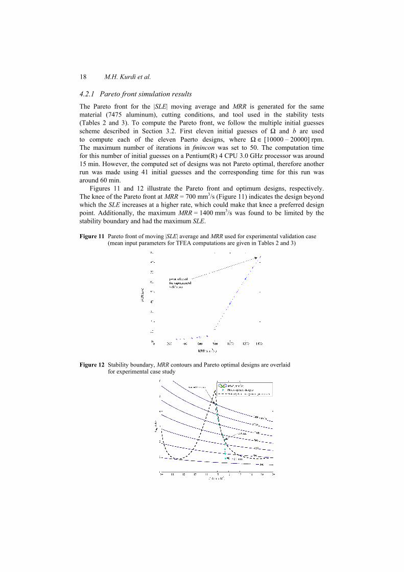
The Pareto front for the |SLE| moving average and MRR is generated for the same material (7475 aluminum), cutting conditions, and tool used in the stability tests (Tables 2 and 3). To compute the Pareto front, we follow the multiple initial guesses scheme described in Section 3.2. First eleven initial guesses of Ω and b are used to compute each of the eleven Paerto designs, where Ω ∈ [10000 – 20000] rpm. The maximum number of iterations in fmincon was set to 50. The computation time for this number of initial guesses on a Pentium(R) 4 CPU 3.0 GHz processor was around 15 min. However, the computed set of designs was not Pareto optimal, therefore another run was made using 41 initial guesses and the corresponding time for this run was around 60 min.

Figures 11 and 12 illustrate the Pareto front and optimum designs, respectively. The knee of the Pareto front at MRR = 700 mm3/s (Figure 11) indicates the design beyond which the SLE increases at a higher rate, which could make that knee a preferred design point. Additionally, the maximum MRR = 1400 mm3/s was found to be limited by the stability boundary and had the maximum SLE.

Figure 11 Pareto front of moving |SLE| average and MRR used for experimental validation case (mean input parameters for TFEA computations are given in Tables 2 and 3)

Figure 12 Stability boundary, MRR contours and Pareto optimal designs are overlaid for experimental case study


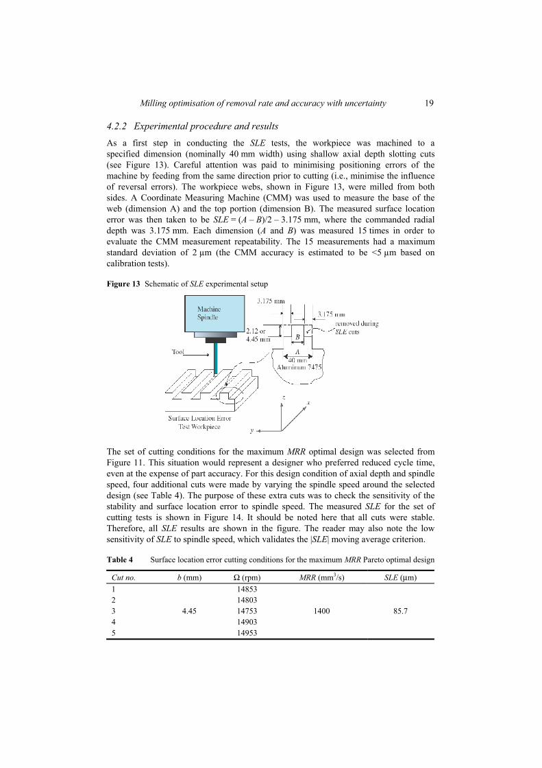
4.2.2 Experimental procedure and results

As a first step in conducting the SLE tests, the workpiece was machined to a specified dimension (nominally 40 mm width) using shallow axial depth slotting cuts (see Figure 13). Careful attention was paid to minimising positioning errors of the machine by feeding from the same direction prior to cutting (i.e., minimise the influence of reversal errors). The workpiece webs, shown in Figure 13, were milled from both sides. A Coordinate Measuring Machine (CMM) was used to measure the base of the web (dimension A) and the top portion (dimension B). The measured surface location error was then taken to be SLE = (A – B)/2 – 3.175 mm, where the commanded radial depth was 3.175 mm. Each dimension (A and B) was measured 15 times in order to evaluate the CMM measurement repeatability. The 15 measurements had a maximum standard deviation of 2 µm (the CMM accuracy is estimated to be <5 µm based on calibration tests).

Figure 13 Schematic of SLE experimental setup

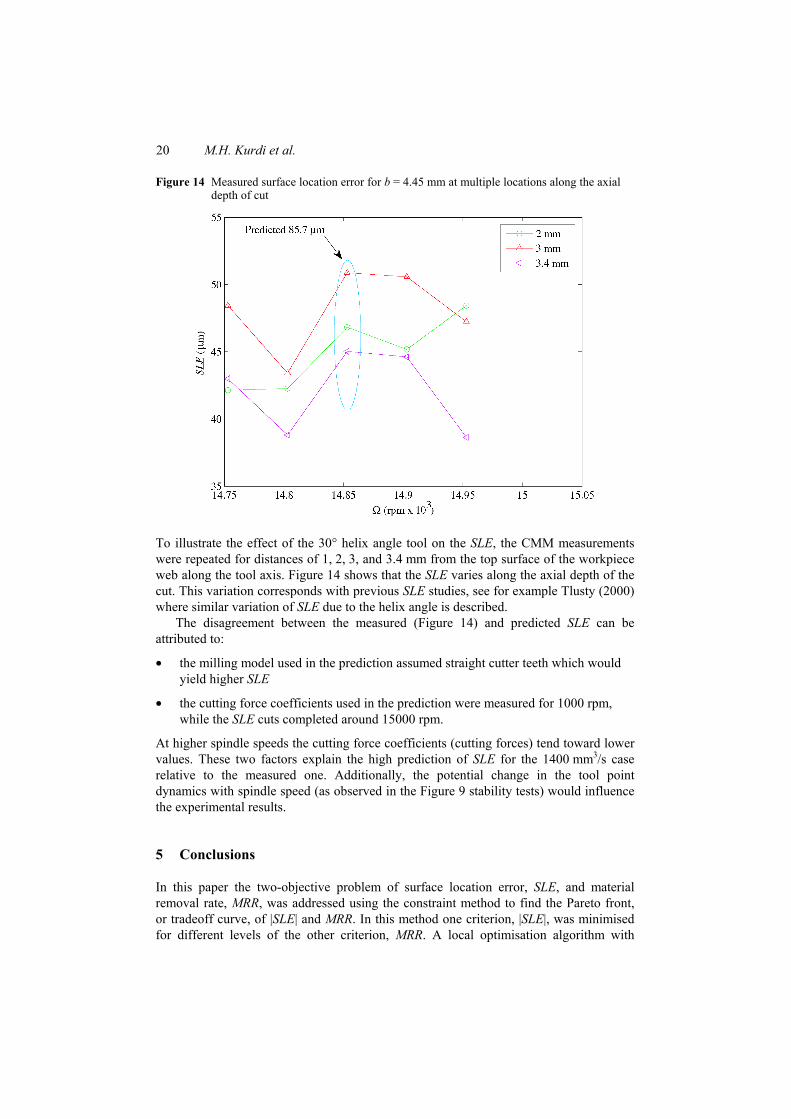
The set of cutting conditions for the maximum MRR optimal design was selected from Figure 11. This situation would represent a designer who preferred reduced cycle time, even at the expense of part accuracy. For this design condition of axial depth and spindle speed, four additional cuts were made by varying the spindle speed around the selected design (see Table 4). The purpose of these extra cuts was to check the sensitivity of the stability and surface location error to spindle speed. The measured SLE for the set of cutting tests is shown in Figure 14. It should be noted here that all cuts were stable. Therefore, all SLE results are shown in the figure. The reader may also note the low sensitivity of SLE to spindle speed, which validates the |SLE| moving average criterion.

Table 4 Surface location error cutting conditions for the maximum MRR Pareto optimal design

Cut no. b (mm) Ω (rpm) MRR (mm3/s) SLE (µm) 1 14853 2 14803 3 4.45 14753 1400 85.7 4 14903 5 14953


Figure 14 Measured surface location error for b = 4.45 mm at multiple locations along the axial depth of cut

To illustrate the effect of the 30° helix angle tool on the SLE, the CMM measurements were repeated for distances of 1, 2, 3, and 3.4 mm from the top surface of the workpiece web along the tool axis. Figure 14 shows that the SLE varies along the axial depth of the cut. This variation corresponds with previous SLE studies, see for example Tlusty (2000) where similar variation of SLE due to the helix angle is described.

The disagreement between the measured (Figure 14) and predicted SLE can be attributed to:

• the milling model used in the prediction assumed straight cutter teeth which would yield higher SLE

• the cutting force coefficients used in the prediction were measured for 1000 rpm, while the SLE cuts completed around 15000 rpm.

At higher spindle speeds the cutting force coefficients (cutting forces) tend toward lower values. These two factors explain the high prediction of SLE for the 1400 mm3/s case relative to the measured one. Additionally, the potential change in the tool point dynamics with spindle speed (as observed in the Figure 9 stability tests) would influence the experimental results.

5 Conclusions

In this paper the two-objective problem of surface location error, SLE, and material removal rate, MRR, was addressed using the constraint method to find the Pareto front, or tradeoff curve, of |SLE| and MRR. In this method one criterion, |SLE|, was minimised for different levels of the other criterion, MRR. A local optimisation algorithm with


multiple initial guesses along the MRR objective was applied. The multi-start search procedure was found to be effective in finding the Pareto optimum as well as in overcoming the effect of objective and constraint first derivative discontinuities. However, the initial implementation of the optimisation formulation indicated the need to be concerned with objective sensitivity. A robust formulation of the |SLE| objective, defined as the moving |SLE| average, was found to be successful in finding operational optima insensitive to spindle speed variation. Finally a Pareto front was calculated for an experimental case study. Tests for a maximum MRR design did not exhibit chatter and the measured surface location error did not show high sensitivity to spindle speed variation. This demonstrated the robustness of the optimisation formulation. Additionally, the computed Pareto front allowed visualisation of the existing tradeoff between the process accuracy and productivity.

In Part 2 of this paper, the measurement procedure used in estimating the mean, variation and correlation of the milling model parameters is described. The variability in the parameters is propagated through the model using sampling methods. The variability in stability boundary and SLE are quantified by calculating the standard deviation of the realised samples. Additionally, the effect of correlation between parameters on the output variability is quantified.

Acknowledgements

The authors gratefully acknowledge partial financial support from the National Science Foundation (DMI-0238019 and CMS-0348288), Office of Naval Research (2003 Young Investigator Program), and TechSolve, Cincinnati, OH. They would also like to recognise Dr. J. Snyder, TechSolve, for his help in collecting portions of the data used in this study.

References Agapiou, J.S. (1992) ‘The optimization of machining operations based on a combined criterion

– part I: the use of combined objectives in single-pass operations’, ASME Journal of Engineering for Industry, Vol. 114, p.500.

Boothroyd, G. and Rusek, P. (1976) ‘Maximum rate of profit criteria in machining’, Journal of Engineering for Industry-Transactions of the ASME, Vol. 98, No. 1, p.217.

Coello Coello, C.A., Lamont, G.B. and Veldhuizen, D.A. (2006) Evolutionary Algorithms for Solving Multi-Objective Problems (Genetic and Evolutionary Computation), Springer-Verlag, NY.

Delio, T., Tlusty, J. and Smith, S. (1992) ‘Use of audio signals for chatter detection and control’, Journal of Engineering for Industry-Transactions of the ASME, Vol. 114, No. 2, p.146.

Deshayes, L., Welsch, L., Donmez, A. and Ivester, R. (2005) ‘Robust optimization for smart machining systems: an enabler for agile manufacturing’, ASME International Mechanical Engineering Congress and Exposition, Orlando, FL.

Ermer, D.S. (1971) ‘Optimization of constrained machining economics problem by geometric programming’, ASME Journal of Engineering for Industry, Vol. 93, p.1067.


Eschenauer, H.A., Koski, J. and Osyczka, A. (1986) Multicriteria Design Optimization: Procedures and Applications, Springer-Verlag, NY.

Garg, N.K., Mann, B.P., Kim, N.H. and Kurdi, M.H. (2007) ‘Stability of a time-delayed differential system with parametric excitation’, ASME Journal of Dynamic Systems, Measurements, and Control, Vol. 129, No. 2, p.125.

Halley, J.E. (1999) Stability of Low Radial Immersion Milling, MSc Thesis, Washington University, St. Louis, MO.

Hati, S.K. and Rao, S.S. (1976) ‘Determination of optimum machining conditions – deterministic and probabilistic approaches’, Journal of Engineering for Industry-Transactions of the ASME, Vol. 98, No. 1, p.354.

Hitomi, K. (1989) ‘Analysis of optimal machining speeds for automatic manufacturing’, International Journal of Production Research, Vol. 27, p.1685.

Juan, H., Yu, S.F. and Lee, B.Y. (2003) ‘The optimal cutting-parameter selection of production cost in HSM for SKD61 tool steels’, International Journal of Machine Tools and Manufacture, Vol. 43, No. 7, p.679.

Kalyanmoy, D. (2001) Multi-Objective Optimization Using Evolutionary Algorithms, John Wiley, West Sussex, England.

Kim, K-K., Kang, M-C., Kim, J-S., Jung, Y-H. and Kim, N-K. (2002) ‘A study on the precision machinability of ball end milling by cutting speed optimization’, Journal of Materials Processing Technology, Vols. 130–131, p.357.

Mann, B.P. (2003) Dynamics of Milling Process, PhD Dissertation, Washington University, St. Louis, MO.

Mann, B.P., Bayly, P.V., Davies, M.A. and Halley, J.E. (2004) ‘Limit cycles, bifurcations, and accuracy of the milling process’, Journal of Sound and Vibration, Vol. 277, Nos. 1–2, p.31.

Mann, B.P., Young, K.A., Schmitz, T.L. and Dilley, D.N. (2005) ‘Simultaneous stability and surface location error predictions in milling’, Journal of Manufacturing Science and Engineering-Transactions of the ASME, Vol. 127, No. 3, p.446.

Miettinen, K. (1999) Nonlinear Multiobjective Optimization, Kluwer Academic Publishers, Boston. Papila, M., Haftka, R.T., Nishida, T. and Sheplak, M. (2006) ‘Piezoresistive microphone design

pareto optimization: tradeoff between sensitivity and noise floor’, Journal of Microelectromechanical Systems, Vol. 156, p.1632.

Rakowska, J., Haftka, R.T. and Watson, L.T. (1991) ‘Tracing the efficient curve for multi-objective control-structure optimization’, Computing Systems in Engineering, Vol. 2, Nos. 5–6, p.461.

Schwier, A.S. (1971) Manual of Political Economy, Translation of the French Edition, McMillan Press Ltd., London-Basingslohe.

Shalaby, M.A. and Riad, M.S. (1988) ‘A linear optimization model for single pass turning operations’, Proceedings of 27th International MATADOR Conference, University of Manchester, Macmillan Education Publishing, Manchester.

Smith, S. and Tlusty, J. (1991) ‘An overview of modeling and simulation of the milling process’, Journal of Engineering for Industry-Transactions of the ASME, Vol. 113, No. 2, p.169.

Tlusty, J. (2000) Manufacturing Processes and Equipment, Prentice-Hall, Upper Saddle River, NJ. Wu, S.M. and Ermer, D. (1966) ‘Maximum profit as the criterion in the determination of the

optimum cutting conditions’, ASME Journal of Engineering for Industry, Vol. 88 p.435.

Website http://www.techsolve.org/.


Nomenclature

a Radial depth of cut (mm) b Axial depth of cut (mm) bi Axial depth corresponding to stability limit at iteration i blim Axial depth at stability limit (mm) C 2 × 2 modal damping matrix Cx Modal viscous damping in x-direction (N.s/m) Cy Modal viscous damping in y-direction (N.s/m) d Tool or cutter diameter (mm) E Total number of elements used to approximate time in the cut

0 ( )f t Time dependent 2 × 1 cutting force coefficient vector

fn Natural frequency (Hz) Fx(t) Total cutting force acting on tool in x-direction (N) Fy(t) Total cutting force acting on tool in y-direction (N) h Feed per tooth (mm/tooth) K 2 × 2 modal stiffness matrix Kc(t) Time dependent 2 × 2 cutting force coefficient matrix Kn Normal cutting force coefficient (N/m2) Kne Edge effiect normal cutting force coefficient (N/m) Kt Tangential cutting force coefficient (N/m2) Kte Edge effect tangential cutting force coefficient (N/m) Kx Modal stiffness in x-direction (N/m) Ky Modal stiffness in y-direction (N/m) Mx Modal mass in x-direction (kg) My Modal mass in y-direction (kg) M 2 × 2 modal mass matrix MRR Material removal rate (mm3/s) N Number of cutter teeth n Tooth passage period number SLE Surface Location Error (µm) x Feed direction

( )X t Two-element position vector for x and y-directions

y Direction normal to feed in the cut plane α Helix angle of cutter (degrees)

ε Bi-section method convergence limit

λk Characteristic multiplier k λmax Magnitude of maximum characteristic multiplier

Ω Spindle speed (rpm)

φ Cutter angle (degrees)


φex Cut exit angle (degrees)

φst Cut entry angle

τ Tooth passing period (s) ζ Damping ratio

mohammad h. kurdi*, tony l. schmitz and raphael t. haftka

Documents