mohammad h. kurdi*, tony l. schmitz and raphael t. …plaza.ufl.edu/mhkurdi/ijmpt_2_2007.pdf · 2...

Int. J. Materials and Product Technology, Vol. x, No. x, xxxx 1

Copyright © 200x Inderscience Enterprises Ltd.

Milling optimisation of removal rate and accuracy with uncertainty: part 2: parameter variation

Mohammad H. Kurdi*, Tony L. Schmitz and Raphael T. Haftka Mechanical and Aerospace Engineering Department, University of Florida, Gainesville, 32611, Florida Fax: +937-656-4945 E-mail: [email protected] E-mail: [email protected] E-mail: [email protected] *Corresponding author

Brian P. Mann Mechanical and Aerospace Engineering Department, University of Missouri, Columbia, MO 65211 E-mail: [email protected]

Abstract: Milling models provide tools for estimating stability and surface location error. Existing models are deterministic, though inherent variations in the model inputs propagate to uncertainty in the model outputs. In this paper the experimental procedures used to estimate the model parameters are presented. The effect of correlation between parameters is addressed. The variability of the stability boundary and surface location errors are determined using Latin Hypercube sampling. It is seen that including the correlation between parameters reduced the output variability by as much as 55% with a minimum reduction of 10%. Comparisons between mean model predictions and experimental results are provided.

Keywords: milling; uncertainty; correlation; stability; multi-response regression.

Reference to this paper should be made as follows: Kurdi, M.H., Schmitz, T.L., Haftka, R.T. and Mann, B.P. (xxxx) ‘Milling optimisation of removal rate and accuracy with uncertainty: part 2: parameter variation’, Int. J. Materials and Product Technology, Vol. x, No. x, pp.xxx–xxx.

Biographical notes: Mohammad H. Kurdi is a National Research Council Postdoctoral Associate at the Air Force Research Laboratory. Mohammad completed his BSc at the University of Jordan and his PhD at University of Florida in 2005. His research interests include multi-objective optimisation, design under uncertainty and advanced computational methods. Current projects are in uncertainty quantification of flutter boundaries in aircraft structures.

Tony L. Schmitz is an Assistant Professor in the Department of Mechanical and Aerospace Engineering at the University of Florida, where he is the Director of the Machine Tool Research Center. His primary interests are in the fields of manufacturing metrology and process dynamics with a current projects in high-speed machining and displacement measuring interferometry. Recent professional recognitions include the National Science Foundation CAREER

2 M.H. Kurdi et al.

award, Office of Naval Research Young Investigator award, and the Society of Manufacturing Engineers Outstanding Young Manufacturing Engineer award. Schmitz received his PhD from the University of Florida in 1999.

Raphael (Rafi) T. Haftka completed his undergraduate education at Technion Israel and his PhD at UC San Diego. He has taught at Technion, Illinois Institute of Technology, and Virginia Tech before coming to the University of Florida in 1995 where he is a Distinguished Professor. His research is in the areas of Structural and Multidisciplinary Optimisation and Design under Uncertainty, which gives him the opportunity and pleasure to collaborate with many colleagues. He has co-authored papers with more than 100 peers in 13 countries. He has authored two textbooks and hundreds of papers, and his work was cited by more than 2500 journal papers.

Brian P. Mann is an Assistant Professor in the Department of Mechanical and Aerospace Engineering at the University of Missouri – Columbia. He received his DSc Degree in 2003 from Washington University St. Louis. Past honours include being awarded the National Defense Science and Engineering Graduate Fellowship and a CAREER Award from the National Science Foundation. His general research interests are in vibration phenomena, non-linear dynamics, and in the influence of time delays on stability.

1 Introduction

In milling operations, models may be used to predict process stability and dimensional accuracy (surface location error) for a specific set of cutting parameters. Selecting optimum cutting parameters that maximise productivity and accuracy is highly desirable. In Part 1 of this paper, optimisation was used to select optimum cutting conditions. Two competing objectives, Material Removal Rate (MRR) and Surface Location Error (SLE) (Schmitz and Ziegert, 1999; Smith and Tlusty, 1991; Kline et al., 1982), were simultaneously considered using a Pareto front, or tradeoff curve. Although the milling model used in the optimisation algorithm (time finite element analysis, or TFEA (Mann et al., 2005; Mann, 2003)) is deterministic, variations in the input parameters of the model limit the confidence in these optimum predictions. Experimental results in Part 1 emphasised the need to account for variations in the input parameters, which include cutting force coefficients (material and process dependent), tool modal parameters, and cutting parameters. Quantifying variations in these values is necessary for the selection of robust optimum designs.

Different types of uncertainties exist in model predictions including (see for example Thoft-Christensen and Baker, 1982):

• physical variations in loads, material properties and dimensions

• lack of information resulting from limited number of experiments

• model limitations which occur due to simplified mathematical representations, unknown boundary conditions and unknown effects of other variables and their interactions.

In this study we account for the first and second types only, with measurement errors representing the source of lack of information. In previous studies (e.g., Guerra et al.,

Milling optimisation of removal rate and accuracy with uncertainty 3

2003; Kim et al., 2003; Rober et al., 1997), uncertainty in the milling process was handled through a posteriori compensation. In Kim et al. (2003) and Rober et al. (1997), the cutting force uncertainty was accommodated using a control system. The force controller was designed to compensate for known process effects and account for the force-feed nonlinearity inherent in metal cutting operations. A relevant study considered uncertainty directly for maximisation of material removal rate in a turning operation, where the confidence intervals of the design variables were obtained using prior knowledge and heuristic methods to find a robust optimum (Deshayes et al., 2005).

We quantify the output variation by propagating the variation of the process parameters through the analysis model. Some of the process parameters are correlated. Considering the physical interdependence of the parameters can lead to different variation in the response. For example, Honda and Antonsson (2003) has considered parameter variation when the parameters are correlated and uncorrelated. Rooney and Biegler (2001) showed the importance of including parameter correlation in design problems by using elliptical joint confidence regions to describe the correlation among the uncertain model parameters. In a recent paper, Becerra and Hernandez (2006) deemed parameter correlation imperative to the proper evaluation of air density uncertainty. In our study, the variation and correlation in the model parameters are measured and propagated through the model using sampling methods. The variation in the output for both correlated and uncorrelated parameters is reported. Results show a noteworthy difference between the responses for correlated and uncorrelated parameters. This enables more accurate quantification of the performance uncertainty and selection of a design that accounts for the inherent input uncertainties a priori.

The objectives of this study are to:

• measure the mean values of the milling model parameters and determine their variation and correlation

• use Monte Carlo and Latin Hypercube sampling methods to propagate the variations

• quantify the stability boundary and SLE uncertainties

• illustrate the significance of accounting for the correlation between parameters on the output variability in the milling model

• compare the experimental case study in Part 1 to the realised sample distribution of stability and SLE.

The paper is arranged as follows. Section 2 provides the theoretical and experimental background for measuring the mean, variation and correlation of the input parameters in the milling model. Section 3 describes the sampling methods used in the confidence interval calculation. Section 4 gives a numerical example for the estimation of SLE and stability boundary distributions and Section 5 outlines the main conclusions of the paper.

2 Model parameter estimation

In this section the mean levels, variation and correlation of the model parameters are estimated for the tool modal parameters, cutting force coefficients and other machining parameters.

4 M.H. Kurdi et al.

2.1 Measurement of tool modal parameters

Modal parameters are used to represent the tool point frequency response function of the tool-holder-spindle-machine system. The tool point frequency response function is typically measured using an impulse force to excite the tool and an accelerometer to measure the response (i.e., impact testing). The time signals of the impulse and response are transformed into the frequency domain using the Fast Fourier Transform. The peak amplitude method (Pandit, 1991; Ewins, 1982) may then be applied to fit the measured frequency response function. In this method, the frequency at the peak of the magnitude of the frequency response function, H (≅ 1/[2ζK]) of a particular mode is taken as the natural frequency, fn, of that mode:

1( ) ,2nH f

Kζ≅ (1)

where the natural frequency is:

1 .2n

KfMπ

= (2)

From equation (1) the damping ratio ζ is estimated from the half power frequencies, f1 and f2, corresponding to:

1,2( ) 1/(2 2 ).H f Kζ= (3)

This enables determination of modal mass, M, damping, C, and stiffness, K, of the tool-holder-spindle-machine for each modelled mode (a rigid workpiece was assumed in this study). It should be noted here that the peak amplitude method is limited to the case where the modes are well separated. However, because the tool used in our experimental study can be approximated as single mode, the method can be applied here.

2.2 Variation and correlation of tool modal parameters

The variation, correlation and mean values of the modal parameters are calculated by repeating the measurement and fitting procedure multiple times. Due to the general symmetry of the tool-holder-spindle assembly, it is expected that the x and y-direction modal parameters should exhibit some level of correlation. Therefore, in sampling from the distribution of potential modal values for uncertainty propagation through the milling model, this correlation should be considered. For example, a random selection of a high stiffness in the x-direction would be expected to correlate with a high stiffness in the y-direction. The correlation between the modal stiffness in the x and y-directions, ,

x yK Kρ

is calculated according to:

1

2 21 1

( )( ),

( ) ( )i i

x y

i i

Qy y x xi

K K Q Qy y x xi i

K K K K

K K K Kρ =

= =

− −=

− −

∑∑ ∑

(4)


where Q is the number of times the experiment is conducted and xK and yK are the mean values. Several factors contribute to the variability in the estimated modal parameters:

• the fitting method

• changes in the tool-holder interface due to tool-holder removal/replacement

• the thermal state of the machine spindle

• the impact testing procedure.

The combined effect of all these factors can be estimated by repeating the measurement under varying conditions. However, the reader may note that this approach does not account for potential impact testing biases (such as accelerometer mass loading or incorrect calibration constants for the transducers) and we have not addressed variations due to removal of the tool from the holder.

2.3 Measurement of cutting force coefficients

A mechanistic model is used to determine the cutting forces. In this approach the cutting forces are expressed as a function of cutting force coefficients. The average milling forces during one tooth period in the x and y-directions is given by Budak et al. (1996) and Altintas (2000):

[ cos(2 ) [2 sin(2 )]] [ sin( ) cos( )]8 2

ex

st

x t n te neNbh NbF K K K K

φ

φ

φ φ φ φ φπ π

= − − + − +

(5)

[ [2 sin(2 )] cos(2 )] [ cos( ) sin( )]8 2

ex

st

y t n te neNbh NbF K K K K

φ

φ

φ φ φ φ φπ π

= − + − +

(6)

where N is the number of teeth on the cutting tool, b is the axial depth, h is the feed per tooth, φ is the cutter angle, and Kt, Kn, Kte and Kne are the tangential, normal, and tangential and normal edge cutting force coefficients, respectively. In slotting tests (see Figure 1(c)), the start and exit angles of the cutter are φst = 0 and φex = 180°, respectively. The average forces per tooth period for this case simplify to:

4x n neNb NbF K h K

π= − − (7a)

.4y t te

Nb NbF K h Kπ

= + (7b)

6 M.H. Kurdi et al.

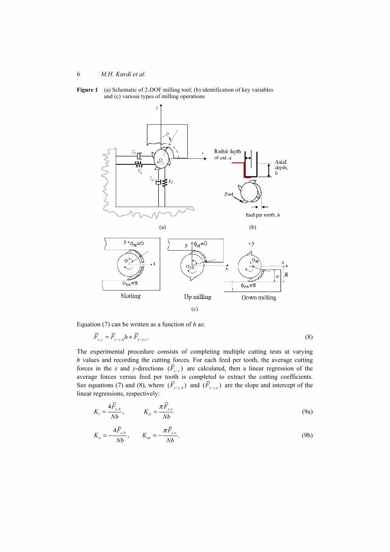
Figure 1 (a) Schematic of 2-DOF milling tool; (b) identification of key variables and (c) various types of milling operations

(a) (b)

(c)

Equation (7) can be written as a function of h as:

, / , / , .x y x y h x y eF F h F= + (8)

The experimental procedure consists of completing multiple cutting tests at varying h values and recording the cutting forces. For each feed per tooth, the average cutting forces in the x and y-directions /( )x yF are calculated, then a linear regression of the average forces versus feed per tooth is completed to extract the cutting coefficients. See equations (7) and (8), where / ,( )x y hF and / ,( )x y eF are the slope and intercept of the linear regressions, respectively:

, ,4,y h y e

t te

F FK K

Nb Nbπ

= = (9a)

, ,4, .x h x e

n ne

F FK K

Nb Nbπ

= − = − (9b)


2.4 Variation and correlation of cutting force coefficients

The linear regression performed in the previous section is a single response analysis. However, the measured responses are the forces in both the x and y-directions during a single measurement (recorded using a dynamometer). This represents a multi-response measurement. Therefore, analysis of the data should take into consideration its multivariate nature, which would provide information regarding potential correlation between the responses. However, it should be noted that both single and multi-response linear regressions give identical estimates of the mean and variation of the fitting parameters. The development of the multi-response model follows the description provided in reference (see Khuri and Cornell, 1996, pp.252–254). If we let Q be the number of times the experiment is conducted and r be the number of response variables (two in our case, i.e., Fx and Fy) measured for each feed per tooth, then the x or y response models can be written in vector form as:

or ,i i i iF i x yβ ε= + =Z (10)

where Fi is a Q × 1 vector of observations of the x or y average cutting force responses, βi is a 2 × 1 vector of unknown constant parameters, and εi is a random error vector associated with the ith response. Equation (10) can be written in matrix form as:

01

2 11

022

12

01 1

,0

1 1

x xx

Q

yy yQ

FQ QF

Q Q

β εββ εβ

×

×

× × = + × ×

Z

Z (11)

where Zi is defined as:

1 1,x y Q Q× ×

= = 1Z Z h (12)

h represents the feed per tooth vector at which the responses are observed and 1 is a vector of ones. The assumption of a simple linear regression applies here. That is, the expected value of εi is, E(εi) = 0. However, the variance-covariance matrix between the responses is not zero; this matrix can be written as:

2

2 .x xy

xy y

σ σσ σ

=

∑ (13)

Therefore, ε (with a 2Q × 1 size) has the following variance-covariance matrix:

Var( ) ,Qε∆ = = ⊗∑ I (14)

where IQ is Q × Q identity matrix and ⊗ is a symbol for the direct (or Kronecker) product of matrices. The direct product of two matrices ∑ and IQ, of sizes 2 × 2 and Q × Q, respectively, gives a 2Q × 2Q matrix which is partitioned as σijIQ where σij is the (i, j)th element of matrix ∑. The best linear unbiased estimate of β = [β01 β11 β02 β12]T is given by Zellner (1962):

1 1 1ˆ ( ) ,T Tβ − − −= ∆ ∆Z Z Z F (15)

8 M.H. Kurdi et al.

where F is the left hand side of equation (11) and Z is the coefficient matrix (matrix size 2Q × 4) of β in equation (11). The variance-covariance matrix of the estimated vector β is:

1 1ˆVar( ) ( ) .Tβ − −= ∆Z Z (16)

Since ∑ is usually unknown, its terms are estimated as (Zellner, 1962): 1 1[ ( ) ][ ( ) ]

ˆ .T T T T T

i Q i i i i Q j j j j jij Q

σ− −− −

=F I Z Z Z Z I Z Z Z Z F

(17)

It should be noted that ˆ ijσ is computed from minimising the residuals (the second term in both bracketed expressions in equation (17) using ordinary least-squares fits of the x and y-directions single response models to their respective data sets. Using the estimate for ∑ in equation (17), an estimate of the variance of β can be obtained. The cutting force coefficients are determined using the linear transformation defined in equation (9):

cutˆ[ ][ ],A β=K (18)

where Kcut = [Kne Kn Kte Kt]T and the matrix A for slotting is:

0 0 0

40 0 0.

0 0 0

40 0 0

Nb

Nb

Nb

Nb

π

π

− −

=

A (19)

Therefore, the variance-covariance matrix of cutting force coefficients can be found as

cutˆVar( ) Var( ) .T β=K A A (20)

Using equation (20) the correlation between the tangential cutting force coefficients, for example, can be written as:

, ,t te

t te

t te

K KK K

K K

σρ

σ σ= (21)

where t teK Kσ is the covariance between the Kt and Kte cutting coefficients and

tKσ and

teKσ are the corresponding standard deviations. As seen in equation (9), some correlation is expected between the coefficients Kt and

Kte and between the coefficients Kn and Kne. This is because each pair depends on the cutting force in a single direction. Again, the reader may note that this approach does not account for potential calibration errors (for the dynamometer in this case).


2.5 Variation in other machining parameters

The uncertainty in spindle speed and radial depth are also considered here. These uncertainties are aleatoric in nature (irreducible). Based on the authors’ experience, a standard deviation of 50 rpm and a coefficient of variation of 0.05% are assumed for the spindle speed and radial depth, respectively. The uncertainties here are assumed due to machine characteristics and process setup and are considered to be constant independent of operating conditions.

3 Uncertainty propagation methods (sampling methods)

In this section we discuss the two methods used in propagating uncertainty from input to output. First, we discuss simple random sampling using the Monte Carlo method and then we describe the more efficient Latin Hypercube sampling method.

3.1 Monte Carlo sampling

In this approach, a random sample of size L is selected from the population of each input parameter. The nominal value (mean) and standard deviation of each input parameter are used to generate a sample from a distribution (we have assumed normal, or Gaussian, distributions). This sample is propagated through the mathematical model to yield statistical information about the model output. In our case the milling model outputs are the axial depth limit, blim, and surface location error. The standard deviations of the predicted blim and SLE are then calculated from the sample output at each spindle speed in the range of interest. An improved sampling method will be discussed next.

3.2 Latin hypercube sampling

This method was originally proposed as a variance reduction technique (see McKay and Beckmann, 1979) in which the estimated variance is asymptotically lower than with simple random sampling (Monte Carlo method) (Cheng and Druzdzel, 2000; Stein, 1987). That is, for the same sample size L, this method gives a lower estimate of the output variance than is possible with the Monte Carlo method. The basic idea of this method is that each value (or range of values) of a variable is represented in the sample, no matter which value turns out to be the most important. In this way, the sampling distribution is divided into a number of strata with a random selection inside each stratum. In the following analysis Latin Hypercube sampling is used to propagate the uncertainty from input to output using both zero correlation and a calculated correlation matrix between parameters.

4 Stability boundary and surface location error variations

The output distribution of the stability boundary and surface location errors were calculated using TFEA in conjunction with the bi-section method for the experimental comparison study presented in Part 1. Using the procedure outlined in Section 2, means, standard deviations and correlations for the tool modal parameters and cutting force coefficients were calculated. Tables 1 and 2 give the tool modal parameter results and

10 M.H. Kurdi et al.

Table 3 gives the cutting force coefficients results. In Table 1 we note that the correlation between the modal mass and stiffness in the x and y-directions, ρM,K, is large which can be explained by the small variations in the natural frequency of the system, see equation (2). Also, the symmetry of the tool explains the high correlation ,x yM Mρ and

,x yC Cρ where:

, ,4 .x y n x yC f Mπζ= (22)

Table 1 Fitted tool modal parameters in x and y-directions. Four impact tests (with five repetitions for each test) were conducted for the same tool. The tool holder was removed from/replaced in the spindle between each test and the thermal state of the spindle was varied. The thermal states corresponded to cold and the condition after running the spindle for 30 s at 5000, 10000 and 20000 rpm. These states are denoted by 1, 2, 3 and 4, respectively

Measurement state Mx (kg) Cx (N.s/m) Kx (N/m × 106) My (kg) Cy (N.s/m) Ky (N/m × 106) 1 0.03 24.34 4.83 0.03 29.09 4.30 2 0.03 22.05 4.38 0.02 37.25 2.60 3 0.03 22.66 4.28 0.02 29.54 2.90 4 0.02 24.18 3.95 0.02 29.85 3.40 µ, mean 0.03 23.31 4.36 0.02 31.43 3.30 σ, standard deviation 0.002 0.976 0.316 0.004 3.368 0.644 µ/σ 0.07 0.04 0.07 0.20 0.11 0.20

Table 2 Correlation coefficient matrix between modal parameters

ρij Mx Cx Kx My Cy Ky Mx 1.00 Cx 0.23 1.00 Kx 0.99 0.13 1.00 My 0.86 0.69 0.80 1.00 Cy –0.09 –0.75 –0.05 –0.50 1.00 Ky 0.66 0.88 0.58 0.95 –0.64 1.00

Table 3 Cutting force coefficients for 7475 aluminum obtained from slotting cutting tests at 1000 rpm, for a 3.05 mm axial depth, and feed per tooth values of 0.025, 0.05, 0.10, and 0.15 mm/tooth. The cut at 0.10 mm/tooth was repeated five times. The correlation matrix between the coefficients was obtained using the multi-response regression

Kt (N/m2 × 106) Kn (N/m2 × 106) Kte (N/m × 102) Kne (N/m × 102) µ 841 253 127 101 σ 21.9 26.6 17 20.7 ρij Kne Kn Kte Kt Kne 1.00 Kn –0.93 1.00 Kte –0.13 0.12 1.00 Kt 0.12 –0.13 –0.93 1.00 Regression P – value 2 × 10–8 8 × 10–5 3 × 10–4 3 × 10–3


Latin Hypercube sampling was then combined with TFEA to calculate stability boundary and SLE confidence intervals. The effect of nonzero correlation between parameters is compared to the case of zero correlation. First, a random sample of size L = 1000 was generated while ignoring the correlation between parameters. Another sample of the same size was generated while considering the correlation between cutting force coefficients and between the tool modal parameters (zero correlation was assumed for the other machining parameters, spindle speed and radial depth). In Figure 2, the stability boundaries of seven uncorrelated samples are shown. The average of the stability boundary peaks of the sample, max ,b was calculated as:

lim1max

max( ( )),

Lijj

b xb

L==

∑ (23)

where i is the input parameter index (total of 12 parameters) and j is the sample index. It is seen that both the peak location (spindle speed) and the magnitude of the peak vary widely. The large variation in peak location means that for a stability diagram obtained by averaging, the individual samples will be greatly smeared and will give the wrong impression of the peak. In Figure 3, the stability boundaries of seven correlated samples show only small variations in the peak location, with larger variations in the peak magnitudes than the peak location. We note here that a fine grid of spindle speeds (50 rpm) is used in generating the boundaries in the figure.

Figure 2 Seven stability boundaries calculated using seven of the 1000 samples of the input parameters generated using Latin Hypercube with no correlation. The mean of 1000 samples peaks, maxb (see equation (23)) is found to be =3.7 mm)


Figure 3 Seven stability boundaries calculated using seven of the 1000 samples of the input parameters generated using Latin Hypercube with correlation. The mean of 1000 samples peaks, maxb (see equation (23)) is found to be =4.8 mm)

The mean of the blim distribution, lim ,b was calculated for the aforementioned cases and compared to blim obtained using the mean values of measured parameters, lim ( )ib x where

( )1/L

i ijjx x L

== ∑ (Tables 1 and 3). A comparison is provided in Figure 4. The first

observation from the figure is that neglecting the correlation gives very different estimation of the mean value of the stability boundary. A comparison between the peak on the graph and the mean value of the peak, equation (23) shows that for the uncorrelated case there is substantial smearing due to the shifting of the peak location. For the correlated case, however, there is much better agreement between the peak of the mean inputs stability boundary and the mean of the peaks of the individual simulations. These do not match exactly due to the effect of the operator non-linearity.1 The stability boundary obtained by using mean properties (solid line in Figure 4 is different from the mean of the stability boundaries. This effect is especially true when the variation in the parameters is large. For example, for the small variation case of Kt (circles in Figure 4) only, limb and lim ( )ib x predictions are nearly identical. However for the large variation

case of My (squares in Figure 4), limb and lim ( )ib x predictions are quite different.

The calculated maxb values stress the importance of correlation. For the uncorrelated case

(Figure 2 and the dotted line in Figure 4), max 3.7 mmb = is substantially higher than the calculated peak of 2.7 mm. This implies that the uncorrelated case underestimates the peak of limb due to horizontal shifts in the stability boundary peaks. For the correlated

case (Figure 3 and the dashed line in Figure 4), max 4.8b = is closer to the calculated peak

of 4.3 mm. This suggests that the correlated result limb provides a better representation of


the physical variability in the input parameters. Note that, aside from this effect, we also have a band of uncertainty around the mean. For simple random sampling, the standard deviation of the estimated sample mean depends on the sample size, L, for example for the axial depth limit, blim:

limlim

1/ 2( ) .ib xb Lσ σ−= (24)

Figure 4 Stability boundary calculated using the mean value of input parameters, ,ix mean of blim distribution considering correlation between parameters and without considering the correlation. The mean of blim considering a coefficient of variation, CV, of 2.6% and 20% in My and Kt (squares and circles, respectively) at selected spindle speeds is also shown

For an L = 1000 sample size, this gives an approximately 3% accuracy. This accuracy is improved for Latin Hypercube sampling (Stein, 1987). With this accuracy in mind, the propagated variation in the stability boundary using the Latin Hypercube method was computed to compare the resulting levels with the accuracy limit imposed by the sample size. Results are provided in Figure 5, which shows the standard deviation,

lim,bσ in the

axial depth limit, blim, both with and without correlation. Clearly the correlation has significantly reduced the variation in the limiting axial depth of stability compared to the zero correlation case. However, in both cases, the percentage of the standard deviation to the mean (see Figure 4) is much higher than 3%. The reduction in standard deviation with the inclusion of correlation is expected since ignoring correlation results in a physically unrealistic sample. For example, while ignoring correlation, the modal stiffness in the x and y-directions for a particular sample may be at the extreme opposite sides of the normal distribution, while we do not expect this to be true in practice. Therefore, neglecting the correlation between tool stiffness values, for example, can overestimate its influence on the stability limit.


Figure 5 Standard deviation of the axial depth limit due to parameter variations. The Latin Hypecube method was used for the correlated and zero correlation cases

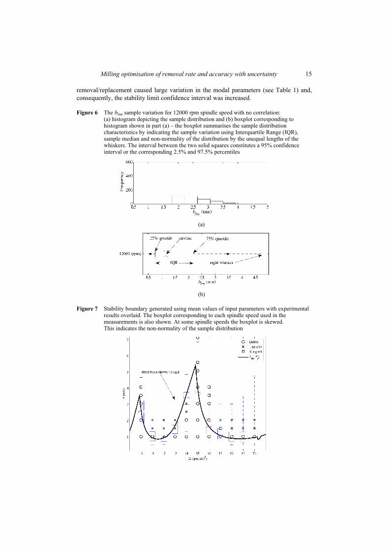
Latin Hypercube sampling with correlation is used to propagate the variation from input to output for the analyses that follow. The histogram of the blim output sample is shown at 12000 rpm in Figure 6(a). The histogram indicates non-normality of the distribution at that spindle speed. The corresponding boxplot (a plot used to show variation and measures of central tendency for a sample) is shown in Figure 6(b). In the figure, the median, 25% and 75% quartiles and two whiskers, which mark the sample extremes, are shown. The unequal lengths of the two whiskers identify the non-normality of the distribution. Also, the Interquartile Range (IQR) gives a measure of the distribution variability. Figure 7 shows the variation in the limiting axial depth as a function of spindle speed with the experimental results presented in Part 1 overlaid. As indicated in the figure, the experimental results generally agree with the median of the sample. In Figure 8 the experimental results are shown with a 95% confidence interval, the interval lies between the 2.5% and 97.5% percentiles of the output distribution. Also shown in the figure is the confidence interval based on two standard deviations of

lim ,b in which the upper bound of this interval agrees with the 97.5% percentile. Though the lower bound gives unrealistic negative blim values, which emphasises that due to the non-linearity in the response, a standard deviation correction may not provide an accurate variation of the response. Furthermore, the confidence interval of the stability limit is also prohibitively large. Accounting for the change in the tool dynamics after tool-holder


removal/replacement caused large variation in the modal parameters (see Table 1) and, consequently, the stability limit confidence interval was increased.

Figure 6 The blim sample variation for 12000 rpm spindle speed with no correlation: (a) histogram depicting the sample distribution and (b) boxplot corresponding to histogram shown in part (a) – the boxplot summarises the sample distribution characteristics by indicating the sample variation using Interquartile Range (IQR), sample median and non-normality of the distribution by the unequal lengths of the whiskers. The interval between the two solid squares constitutes a 95% confidence interval or the corresponding 2.5% and 97.5% percentiles

(a)

(b)

Figure 7 Stability boundary generated using mean values of input parameters with experimental results overlaid. The boxplot corresponding to each spindle speed used in the measurements is also shown. At some spindle speeds the boxplot is skewed. This indicates the non-normality of the sample distribution


Figure 8 A 95% stability limit confidence interval with experimental results overlaid. The interval is based on 2.5% and 97.5% percentiles calculated from the distribution of the output sample. A two standard deviation interval is also shown – the upper limit of the standard deviation interval generally agrees with the 97.5% percentile

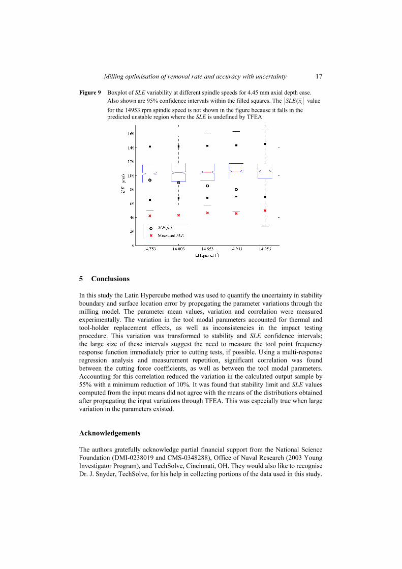
The SLE results from the experimental case study presented in Part 1 (see Table 4) are shown in Figure 9 with the SLE boxplots overlaid. It should be noted here that, because SLE is undefined in the unstable region, only the SLE values of the sample in the stable domain are shown in the boxplot. In Figure 9, it is seen that the variation in the SLE is nearly constant for the five cases considered. It is also seen that the prediction SLE sample median is larger than the experimental results. Although the bounds of the numerical SLE sample depend on the sample size, we believe the discrepancy is dominated by modelling simplifications rather than input value variations. As noted in Part 1, TFEA does not include the effects of the cutting teeth helix angle and we have assumed that the system dynamics and cutting force coefficients do not vary with spindle speed. The figure also identifies the difference between the calculated SLE using the mean parameters, (shown as circles), and the median or mean SLE of the sample. The notch in the figure indicates that the SLE median is essentially constant between consecutive spindle speeds. This result, combined with the small variation in the experimental results, validates the robustness of the maximum MRR (1400 mm3/s with a 4.45 mm axial depth) optimum design.

Table 4 Surface location error cutting conditions for maximum MRR Pareto optimal design (the first cut listed) with four extra cuts at different spindle speeds

Cut no. b (mm) Ω (rpm) MRR (mm3/s) SLE (µm)

1 14853 2 14803 3 4.45 14753 1400 85.7 4 14903 5 14953


Figure 9 Boxplot of SLE variability at different spindle speeds for 4.45 mm axial depth case. Also shown are 95% confidence intervals within the filled squares. The ( iSLE x value for the 14953 rpm spindle speed is not shown in the figure because it falls in the predicted unstable region where the SLE is undefined by TFEA

5 Conclusions

In this study the Latin Hypercube method was used to quantify the uncertainty in stability boundary and surface location error by propagating the parameter variations through the milling model. The parameter mean values, variation and correlation were measured experimentally. The variation in the tool modal parameters accounted for thermal and tool-holder replacement effects, as well as inconsistencies in the impact testing procedure. This variation was transformed to stability and SLE confidence intervals; the large size of these intervals suggest the need to measure the tool point frequency response function immediately prior to cutting tests, if possible. Using a multi-response regression analysis and measurement repetition, significant correlation was found between the cutting force coefficients, as well as between the tool modal parameters. Accounting for this correlation reduced the variation in the calculated output sample by 55% with a minimum reduction of 10%. It was found that stability limit and SLE values computed from the input means did not agree with the means of the distributions obtained after propagating the input variations through TFEA. This was especially true when large variation in the parameters existed.

Acknowledgements

The authors gratefully acknowledge partial financial support from the National Science Foundation (DMI-0238019 and CMS-0348288), Office of Naval Research (2003 Young Investigator Program), and TechSolve, Cincinnati, OH. They would also like to recognise Dr. J. Snyder, TechSolve, for his help in collecting portions of the data used in this study.


References Altintas, Y. (2000) Manufacturing Automation: Metal Cutting Mechanics, Machine Tool

Vibrations, and CNC Design, Cambridge University Press, New York. Becerra, L.O. and Hernandez, I. (2006) ‘Evaluation of the air density uncertainty: the effect of the

correlation of input quantities and higher order terms in the Taylor series expansion’, Measurement Science and Technology, Vol. 17, No. 10, p.2545.

Budak, E., Altintas, Y. and Armarego, E.J.A. (1996) ‘Prediction of milling force coefficients from orthogonal cutting data’, Journal of Manufacturing Science and Engineering-Transactions of the ASME, Vol. 118, No. 2, p.216.

Cheng, J. and Druzdzel, M.J. (2000) ‘Latin hypercube sampling in Bayesian networks’, Thirteenth International Florida Artificial Intelligence Research Society, AAAI Press, Menlo Park, CA.

Deshayes, L., Welsch, L., Donmez, A. and Ivester, R. (2005) Robust Optimization for Smart Machining Systems: An Enabler for Agile Manufacturing, ASME International Mechanical Engineering Congress and Exposition, Orlando, FL.

Ewins, D.J. (1982) Modal Testing: Theory and Practice, John Wiley & Sons Inc., New York. Guerra, R.E.H., Schmitt-Braess, G., Haber, R.H., Alique, A. and Alique, J.R. (2003) ‘Using circle

criteria for verifying asymptotic stability in pl-like fuzzy control systems: application to the milling process’, IEE Proceedings-Control Theory and Applications, Vol. 150, No. 6, p.619.

Honda, T. and Antonsson, E.K. (2003) ‘Preferences and correlated uncertanties in engineering design’, Proceedings of the ASME Design Engineering Technical Conference, Vol. 3, p.805.

Khuri, A.I. and Cornell, J.A. (1996) Response Surfaces: Design and Analysis, Marcel Dekker Inc., New York.

Kim, S.I., Landers, R.G. and Ulsoy, A.G. (2003) ‘Robust machining force control with process compensation’, Journal of Manufacturing Science and Engineering-Transactions of the ASME, Vol. 125, No. 3, p.423.

Kline, W.A., Devor, R.E. and Shareef, I.A. (1982) ‘The prediction of surface accuracy in end milling’, Journal of Engineering for Industry-Transactions of the ASME, Vol. 104, No. 3, p.272.

Mann, B.P. (2003) Dynamics of Milling Process, PhD Dissertation, Washington University, St. Louis, MO.

Mann, B.P., Young, K.A., Schmitz, T.L. and Dilley, D.N. (2005) ‘Simultaneous stability and surface location error predictions in milling’, Journal of Manufacturing Science and Engineering-Transactions of the ASME, Vol. 127, No. 3, p.446.

McKay, M.D. and Beckmann, R.J. (1979) ‘A comparison of three methods for selecting values of input variables in the analysis of output from a computer code’, Technometrics, Vol. 21, No. 2, p.239.

Pandit, S.M. (1991) Modal and Spectrum Analysis: Data Dependent Systems in State Space, John Wiley & Sons Inc., New York.

Rober, S.J., Shin, Y.C. and Nwokah, O.D.I. (1997) ‘A digital robust controller for cutting force control in the end milling process’, Journal of Dynamic Systems Measurement and Control-Transactions of the ASME, Vol. 119, No. 2, p.146.

Rooney, W.C. and Biegler, L.T. (2001) ‘Incorporating joint confidence regions into design under uncertainty’, Computers and Chemical Engineering, Vol. 23, No. 10, p.1563.

Schmitz, T. and Ziegert, J. (1999) ‘Examination of surface location error due to phasing of cutter vibrations’, Precision Engineering-Journal of the American Society for Precision Engineering, Vol. 23, No. 1, p.51.

Smith, S. and Tlusty, J. (1991) ‘An overview of modeling and simulation of the milling process’, Journal of Engineering for Industry-Transactions of the ASME, Vol. 113, No. 2, p.169.

Stein, M. (1987) ‘Large sample properties of simulations using Latin hypercube sampling’, Technometrics, Vol. 29, No. 2, p.143.


Thoft-Christensen, P. and Baker, M.J. (1982) Structural Reliability Theory and its Applications, Springer-Verlag, Berlin, New York, p.xiii.

Zellner, A. (1962) ‘An efficient method of estimating seemingly unrelated regressions and tests for aggregation bias’, Journal of American Statistic Association, Vol. 57, p.348.

Note 1As an example, consider the case of propagating a mean zero normal distribution of samples, x, through the nonlinear absolute value operator, y = |x|. Clearly, the mean value of ( 0)y y > is not

equal to 0.x = Further, the greater spread of x, the higher the disagreement between y and x .

Nomenclature

A Slotting transformation matrix a Radial depth (mm) b Axial depth (mm) bi Root corresponding to stability limit at iteration i (mm) blim Axial depth at stability limit (mm)

maxb Average of the stability boundaries peaks of the sample

Cx Modal damping in x-direction (N.s/m) Cy Modal damping in y-direction (N.s/m) CV Coefficient of Variation F Vector of average observed cutting forces for x and y-directions (N) Fi Average observed cutting force for response i (N) Fx Observed cutting force in x-direction (N) Fy Observed cutting force in y-direction (N)

xF Average cutting force in x-direction (N)

yF Average cutting force in y-direction (N)

/ ,x y hF Average cutting force per chip load (N/m)

/ ,x y eF Average edge cutting force (N)

fn Natural frequency (Hz) f1,2 Half power frequencies (Hz) h Feed per tooth (mm/tooth) H Feed per tooth IQ Identity matrix of size Q Kt Tangential cutting force coefficient (N/m2) Kn Normal cutting force coefficient (N/m2) Kte Tangential edge cutting force coefficient (N/m) Kne Normal edge cutting force coefficient (N/m)


K Modal stiffness (N/m) Kcut Vector of cutting force coefficient (N/m2) Kx Modal stiffness in x-direction (N/m) Ky Modal stiffness in y-direction (N/m) L Sample size MRR Material removal rate (mm3/s) Mx Modal mass in x-direction My Modal mass in y-direction N Number of teeth on the cutting tool Q Number of times the experiment is conducted SLE Surface location error (µm) Var Variance-covariance matrix of a vector

ix Mean of milling parameter xi

y y-direction Zi Coefficient matrix of size (Q × 2) Z Coefficient matrix of size (2Q × 4)

β Unbiased estimate of β

β Vector of unknown constant parameters

εi Random error vector associated with ith response

φ Cutter angle (degrees)

φst Cutter angle at start of cut (degrees)

φex Cutter angle at exit of cut (degrees)

Ω Spindle speed (rpm)

ρ Correlation factor

∑ Variance-covariance matrix

σi Standard deviation of generic parameter i

limbσ Standard deviation of axial depth limit

σij Covariance between i and j

ˆ ijσ Estimate of σij

ζ Damping ratio

mohammad h. kurdi*, tony l. schmitz and raphael t. …plaza.ufl.edu/mhkurdi/ijmpt_2_2007.pdf · 2...

Documents