Monetary and Fiscal Policies Interactions in Mexico: 1981 – 2016

Sebastian Cadavid Sánchez André C. Martínez Fritscher Alberto Ortiz Bolaños CEMLA BID CEMLA & EGADE

5th World Bank – Banco de España Research Conference

“Macroeconomic Policies, Output Fluctuations, and Long-Term Growth” June 4 and 5, 2018

The views expressed in this presentation are those of the author and not necessarily those of BID, CEMLA or EGADE Business School.

Inflation, ex-post real interest rates and debt to GDP in Mexico: 1981 - 2016

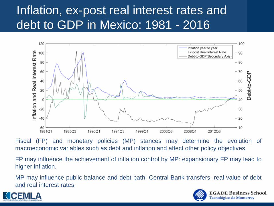
Fiscal (FP) and monetary policies (MP) stances may determine the evolution of macroeconomic variables such as debt and inflation and affect other policy objectives.

FP may influence the achievement of inflation control by MP: expansionary FP may lead to higher inflation.

MP may influence public balance and debt path: Central Bank transfers, real value of debt and real interest rates.

Inflation, central bank legislation, fiscal rules and fiscal councils

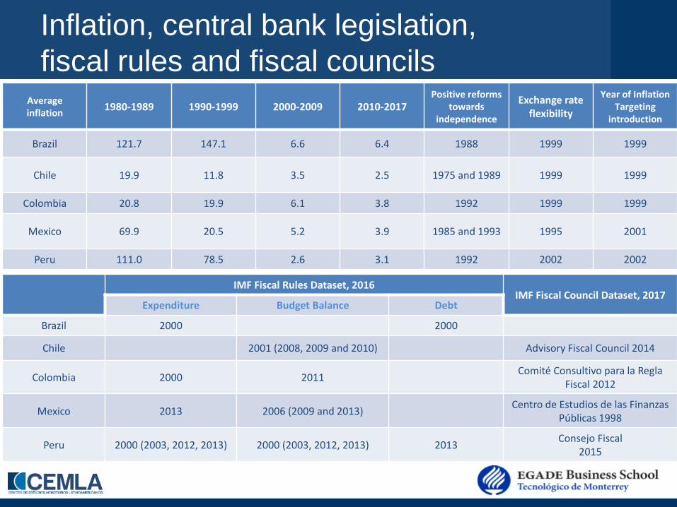
IMF Fiscal Rules Dataset, 2016 IMF Fiscal Council Dataset, 2017

Expenditure Budget Balance Debt

Brazil 2000 2000

Chile 2001 (2008, 2009 and 2010) Advisory Fiscal Council 2014

Colombia 2000 2011 Comité Consultivo para la Regla Fiscal 2012

Mexico 2013 2006 (2009 and 2013) Centro de Estudios de las Finanzas Públicas 1998

Peru 2000 (2003, 2012, 2013) 2000 (2003, 2012, 2013) 2013 Consejo Fiscal 2015

Average inflation 1980-1989 1990-1999 2000-2009 2010-2017

Positive reforms towards

independence

Exchange rate flexibility

Year of Inflation Targeting

introduction

Brazil 121.7 147.1 6.6 6.4 1988 1999 1999

Chile 19.9 11.8 3.5 2.5 1975 and 1989 1999 1999

Colombia 20.8 19.9 6.1 3.8 1992 1999 1999

Mexico 69.9 20.5 5.2 3.9 1985 and 1993 1995 2001

Peru 111.0 78.5 2.6 3.1 1992 2002 2002

This paper

• What we do? Analyze the role of fiscal and monetary policies in the determination of inflation and government debt in Mexico during the 1981-2016 period.

• How we do it? Estimating a Markov-switching DSGE model.

• What we find? – We identify five different periods of fiscal and monetary policy

interactions, which are congruent with a historical account of the Mexican monetary and fiscal policy mix during the past 35 years.

– Counterfactual exercises show that the low-frequency evolution of inflation is mainly determined by the monetary policy stance, while the low-frequency evolution of debt is mainly determined by the fiscal policy stance.

– We show that if monetary dominance had prevailed throughout the whole period, average inflation would have been 13.2% rather than the 20.4% observed. On the other hand, complete fiscal dominance would have implied an average inflation of 42% and an average debt five times larger than the figure observed.

Policy Regimes: Active / Passive FP and MP

Policy regimes: objectives, instruments and stances

• In our setting, policies have the following objectives: 1. FP seeks to smooth distorting taxes. 2. MP controls inflation. • Policies may be active or passive, in function of the restrictions they face:

– An active policy authority is free to pursue its objectives unconstrained by the state of government debt.

– A passive policy authority responds to debt shocks. • Active fiscal policy (AF) implies that taxes don’t respond to debt level,

so fiscal authority isn’t concerned to fulfill the intertemporal public budget constraint and debt follows a non-stationary process, impacting inflation.

• Active monetary policy (AM) means that Central Bank has a high reaction of the interest rate to inflation. It doesn’t allow inflation to deflate real value of debt .

Policy regimes: Leeper 1991

Monetary/Fiscal policy space is composed by four regimes (Leeper, 1991 JME): 1. Monetary dominance (AM/PF): FP guarantees future surpluses to

cover debt, even in presence of fiscal shocks. MP focuses on inflation.

2. Fiscal dominance (PM/AF): FP impacts inflation as it doesn’t satisfy intertemporal budget constraint. MP accommodates to diminish debt and allows inflation.

3. Both active (AM/AF): FP and MP determines inflation but it is an unstable policy mix as it doesn’t exist a bounded debt equilibrium.

4. Both passive (PM/PF): FP and MP stabilize debt and none focuses on inflation. Indeterminate equilibrium with multiple solution.

Relative power between policies given by the institutional framework (e.g. fiscal rules or Central Bank autonomy) may explain how regimes evolve.

Model

Model: summary

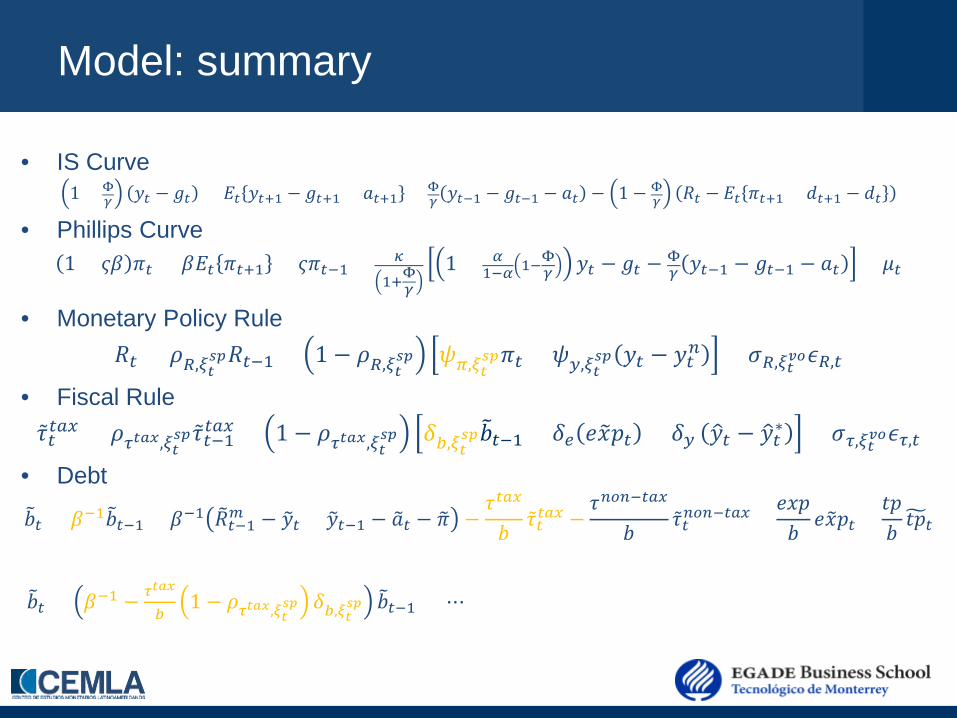
• IS Curve 1 + Φ

𝛾 𝑦𝑡 − 𝑔𝑡 = 𝐸𝑡 𝑦𝑡+1 − 𝑔𝑡+1 + 𝑎𝑡+1 + Φ𝛾 𝑦𝑡−1 − 𝑔𝑡−1 − 𝑎𝑡 − 1 − Φ

𝛾 𝑅𝑡 − 𝐸𝑡 𝜋𝑡+1 + 𝑑𝑡+1 − 𝑑𝑡

• Phillips Curve 1 + 𝜍𝜍 𝜋𝑡 = 𝜍𝐸𝑡 𝜋𝑡+1 + 𝜍𝜋𝑡−1 + 𝜅

1+Φ𝛾1 + 𝛼

1−𝛼 1−Φ𝛾 𝑦𝑡 − 𝑔𝑡 − Φ𝛾 𝑦𝑡−1 − 𝑔𝑡−1 − 𝑎𝑡 + 𝜇𝑡

• Monetary Policy Rule 𝑅𝑡 = 𝜌𝑅,𝜉𝑡

𝑠𝑠𝑅𝑡−1 + 1 − 𝜌𝑅,𝜉𝑡𝑠𝑠 𝜓𝜋,𝜉𝑡

𝑠𝑠𝜋𝑡 + 𝜓𝑦,𝜉𝑡𝑠𝑠 𝑦𝑡 − 𝑦𝑡𝑛 + 𝜎𝑅,𝜉𝑡

𝑣𝑣𝜖𝑅,𝑡

• Fiscal Rule �̃�𝑡𝑡𝑡𝑡 = 𝜌𝜏𝑡𝑡𝑡,𝜉𝑡

𝑠𝑠�̃�𝑡−1𝑡𝑡𝑡 + 1 − 𝜌𝜏𝑡𝑡𝑡,𝜉𝑡𝑠𝑠 𝛿𝑏,𝜉𝑡

𝑠𝑠𝑏�𝑡−1 + 𝛿𝑒 𝑒𝑥�𝑝𝑡 + 𝛿𝑦 𝑦�𝑡 − 𝑦�𝑡∗ + 𝜎𝜏,𝜉𝑡𝑣𝑣𝜖𝜏,𝑡

• Debt

𝑏�𝑡 = 𝜍−1𝑏�𝑡−1 + 𝜍−1 𝑅�𝑡−1𝑚 − 𝑦�𝑡 + 𝑦�𝑡−1 − 𝑎�𝑡 − 𝜋� −𝜏𝑡𝑡𝑡

𝑏�̃�𝑡𝑡𝑡𝑡 −

𝜏𝑛𝑛𝑛−𝑡𝑡𝑡

𝑏�̃�𝑡𝑛𝑛𝑛−𝑡𝑡𝑡 +

𝑒𝑥𝑝𝑏

𝑒𝑥�𝑝𝑡 +𝑡𝑝𝑏𝑡𝑝�𝑡

𝑏�𝑡 = 𝜍−1 − 𝜏𝑡𝑡𝑡

𝑏1 − 𝜌𝜏𝑡𝑡𝑡,𝜉𝑡

𝑠𝑠 𝛿𝑏,𝜉𝑡𝑠𝑠 𝑏�𝑡−1 + ⋯

Solution and estimation

Estimation In the estimation, we allow for two possible values for every relevant policy parameter:

For fiscal policy, we obtain the high (PF) and low (AF) tax rate response to debt.

• Passive �̃�𝑡𝑡𝑡𝑡 = 0.79�̃�𝑡−1𝑡𝑡𝑡 + 1 − 0.79 0.0624𝑏�𝑡−1 + 0.09 𝑒𝑥�𝑝𝑡 + 0.15 𝑦�𝑡 − 𝑦�𝑡∗

• Active �̃�𝑡𝑡𝑡𝑡 = 0.73�̃�𝑡−1𝑡𝑡𝑡 + 1 − 0.73 0.0003𝑏�𝑡−1 + 0.09 𝑒𝑥�𝑝𝑡 + 0.15 𝑦�𝑡 − 𝑦�𝑡∗ For monetary policy, we estimate the low (PM) and high (AM) interest rate sensitivity to inflation.

• Passive 𝑅𝑡 = 0.58𝑅𝑡−1 + 1 − 0.58 0.79𝜋𝑡 + 0.66 𝑦𝑡 − 𝑦𝑡𝑛

• Active 𝑅𝑡 = 0.55𝑅𝑡−1 + 1 − 0.55 1.81𝜋𝑡 + 0.94 𝑦𝑡 − 𝑦𝑡𝑛

Smoothed probabilities 1981Q1 – 1988Q2

1988Q3 – 1995Q1

1995Q2 – 1998Q4

1999 Q1 – 2008 Q3

2008 Q4 – 2016 Q4

Historical Narrative

I. 1981Q1 – 1988Q2: PM / AF

1986 1991 1996 2001 2006 2011 2016

Inflation

Debt / GDP

0

20

40

60

120

100

1981

80

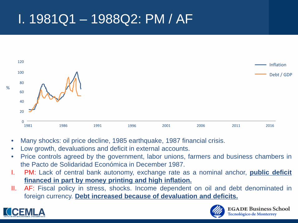
• Many shocks: oil price decline, 1985 earthquake, 1987 financial crisis. • Low growth, devaluations and deficit in external accounts. • Price controls agreed by the government, labor unions, farmers and business chambers in

the Pacto de Solidaridad Económica in December 1987. I. PM: Lack of central bank autonomy, exchange rate as a nominal anchor, public deficit

financed in part by money printing and high inflation. II. AF: Fiscal policy in stress, shocks. Income dependent on oil and debt denominated in

foreign currency. Debt increased because of devaluation and deficits.

%

II. 1988Q3 – 1995Q1: AM / PF PM / AF

1986 1991 1996 2001 2006 2011 2016

Inflation

Debt / GDP

0

20

40

60

120

100

1981

80

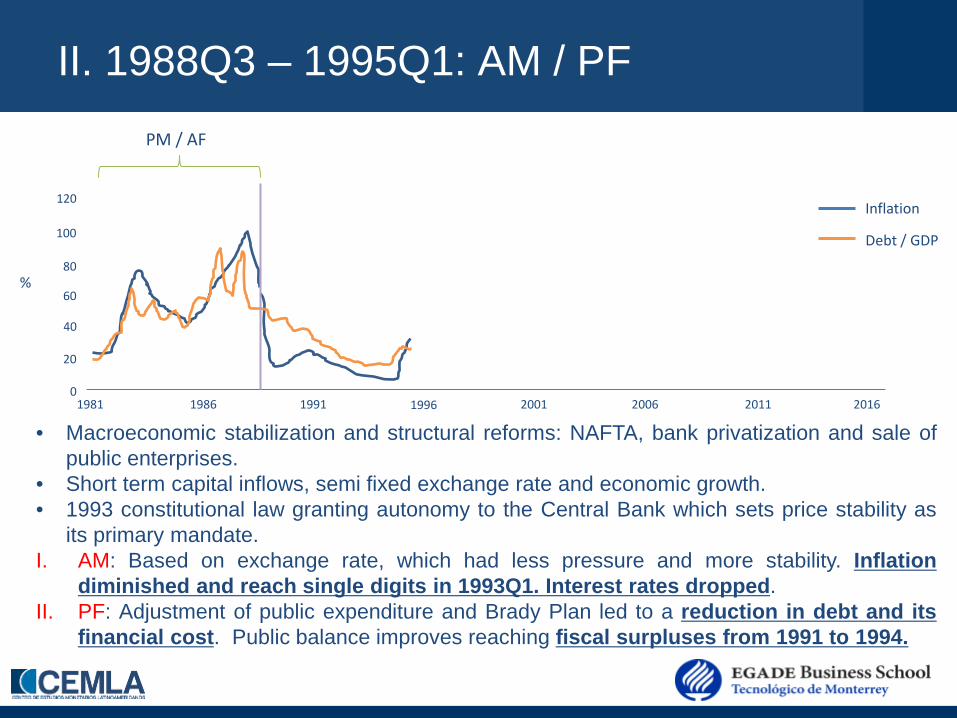
• Macroeconomic stabilization and structural reforms: NAFTA, bank privatization and sale of public enterprises.

• Short term capital inflows, semi fixed exchange rate and economic growth. • 1993 constitutional law granting autonomy to the Central Bank which sets price stability as

its primary mandate. I. AM: Based on exchange rate, which had less pressure and more stability. Inflation

diminished and reach single digits in 1993Q1. Interest rates dropped. II. PF: Adjustment of public expenditure and Brady Plan led to a reduction in debt and its

financial cost. Public balance improves reaching fiscal surpluses from 1991 to 1994.

%

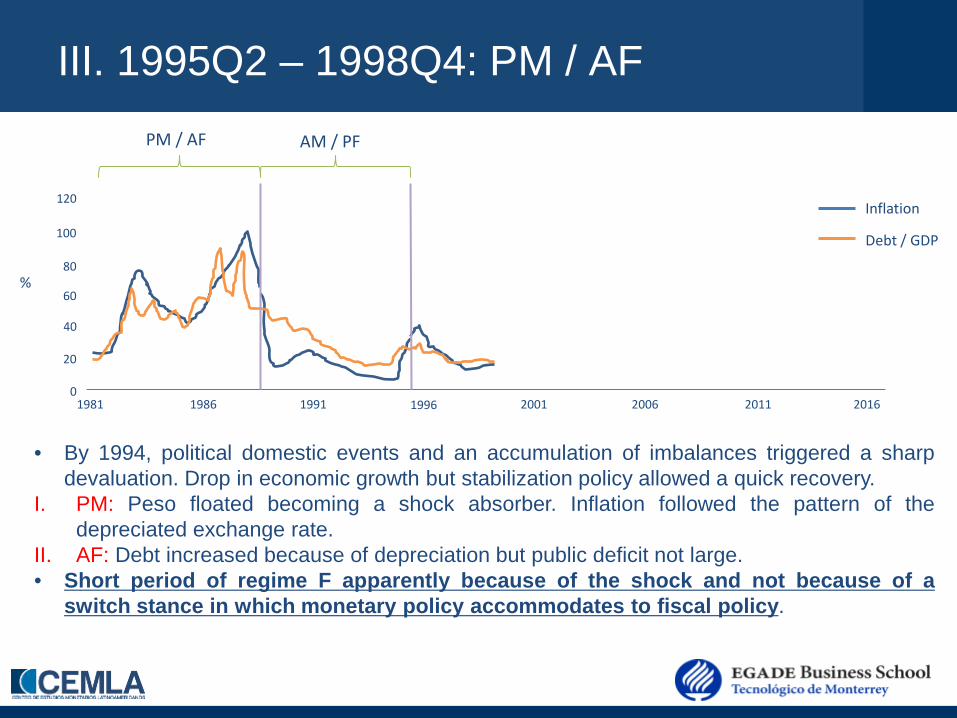
III. 1995Q2 – 1998Q4: PM / AF PM / AF AM / PF

1986 1991 1996 2001 2006 2011 2016

Inflation

Debt / GDP

0

20

40

60

120

100

1981

80

• By 1994, political domestic events and an accumulation of imbalances triggered a sharp devaluation. Drop in economic growth but stabilization policy allowed a quick recovery.

I. PM: Peso floated becoming a shock absorber. Inflation followed the pattern of the depreciated exchange rate.

II. AF: Debt increased because of depreciation but public deficit not large. • Short period of regime F apparently because of the shock and not because of a

switch stance in which monetary policy accommodates to fiscal policy.

%

IV. 1999Q1 – 2008Q3: AM / PF PM / AF PM / AF AM / PF

1986 1991 1996 2001 2006 2011 2016

Inflation

Debt / GDP

0

20

40

60

120

100

1981

80 %

• Economic growth and stability in exchange rate. I. AM: Central Bank switched to an inflation target regime, linking more directly inflation and

interest rates. Inflation became low, less persistent, predictable and stable. II. PF: Fiscal policy incurred in low deficits favored by high oil prices, allowing a declining

path of debt, reaching historical minimums. The 2006 Federal Budget and Fiscal Responsibility Law (LFPRH acronym in Spanish), which among other things set a zero fiscal deficit rule, but with escape clause.

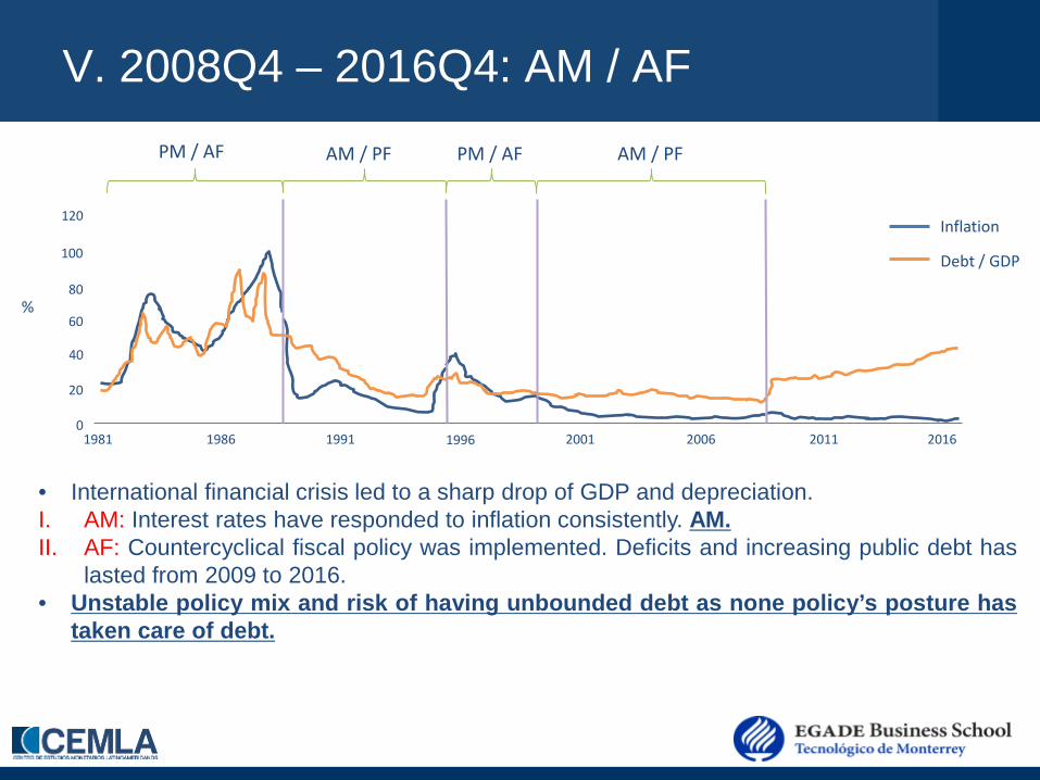
V. 2008Q4 – 2016Q4: AM / AF PM / AF PM / AF AM / PF AM / PF

1986 1991 1996 2001 2006 2011 2016

Inflation

Debt / GDP

0

20

40

60

120

100

1981

80 %

• International financial crisis led to a sharp drop of GDP and depreciation. I. AM: Interest rates have responded to inflation consistently. AM. II. AF: Countercyclical fiscal policy was implemented. Deficits and increasing public debt has

lasted from 2009 to 2016. • Unstable policy mix and risk of having unbounded debt as none policy’s posture has

taken care of debt.

Counterfactuals

• We run two counterfactuals that allow us to understand better the role of expectations, policy mix and shocks in the evolution of the macroeconomic variables. We suppose what it would have happened if:

1. Fiscal and monetary policy regime had stayed within a single regime in the whole sample, 1981 – 2016.

Counterfactual single regime

• In a PM/PF regime, inflation would have been in average higher (49) and debt lower (-62).

• Fiscal dominance would have led to both higher inflation (42) and debt (154).

• Monetary dominance would have resulted in both lower inflation (13) and debt (-57).

• In an AM/AF regime inflation would have been lower (15) and debt higher (202).

• Counterfactuals illustrate the relevance of macroeconomic policy stance for the evolution of macro variables.

Sample averages: Inflation: 20%

Debt: 31%

Counterfactuals

• We run two counterfactuals that allow us to understand better the role of expectations, policy mix and shocks in the evolution of the macroeconomic variables. We suppose what it would have happened if:

1. Fiscal and monetary policy regime had stayed within a single regime in the whole sample, 1981 - 2016.

2. Around each regime switch, 1988Q3, 1995Q2, 1999Q1 and 2008Q4:

a) The regime changed and there was full credibility (100% probability of remaining in the new regime).

b) The regime had not changed remaining in the status-quo (100% probability of remaining in the previous regime).

c) The regime changed but there was no credibility (0% probability of remaining in the new regime).

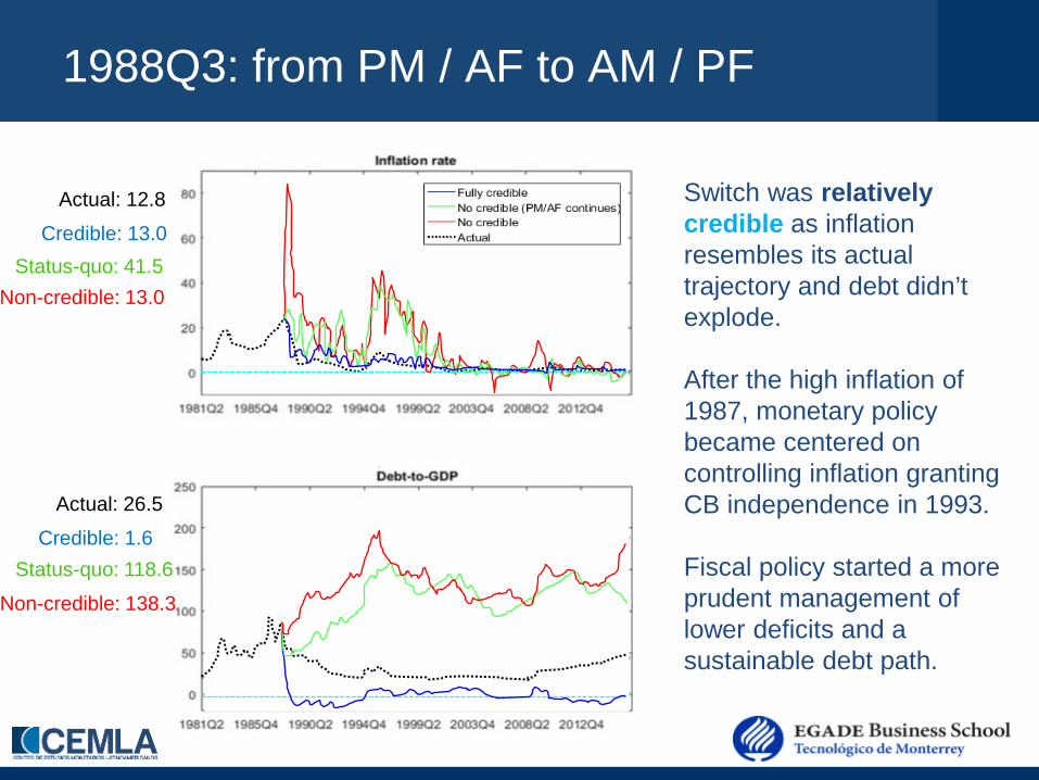
1988Q3: from PM / AF to AM / PF

Switch was relatively credible as inflation resembles its actual trajectory and debt didn’t explode. After the high inflation of 1987, monetary policy became centered on controlling inflation granting CB independence in 1993. Fiscal policy started a more prudent management of lower deficits and a sustainable debt path.

Actual: 12.8

Credible: 13.0 Status-quo: 41.5

Non-credible: 13.0

Actual: 26.5

Non-credible: 138.3

Credible: 1.6 Status-quo: 118.6

1995Q2: from AM / PF to PM / AF

Regime switch was not credible, with variables moving very closely to the AM/PF status-quo trajectory. Otherwise, inflation would have been much larger and debt would have exploded. New regime originated by a shock and not a real switch in policy stances.

Actual: 8.4

Credible: 19.2

Actual: 23.9

Credible: 64.8

Status-quo: 8.4 Non-credible: 6.4

Status-quo: 17.2

Non-credible: 16.7

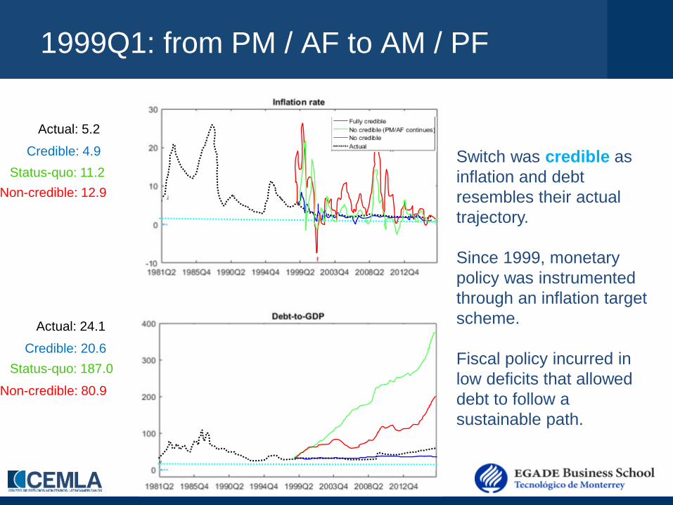
1999Q1: from PM / AF to AM / PF

Switch was credible as inflation and debt resembles their actual trajectory. Since 1999, monetary policy was instrumented through an inflation target scheme. Fiscal policy incurred in low deficits that allowed debt to follow a sustainable path.

Actual: 5.2

Actual: 24.1

Credible: 20.6

Status-quo: 11.2 Non-credible: 12.9

Status-quo: 187.0

Non-credible: 80.9

Credible: 4.9

2008Q4: from AM / PF to AM / AF Switch was not credible as, fiscal authority commitment of reducing deficit in the following years was credible according to the AM/PF status-quo. Monetary policy has kept focusing in inflation control. In the following years, need of change of regime: perhaps from the fiscal side. MP has been active since 1988, except for a couple of years: autonomy of central bank has shown to be critical to control inflation and avoid fiscal dominance.

Actual: 3.8

Actual: 32.1

Credible: 47.5

Status-quo: 3.5 Non-credible: 3.3

Status-quo: 26.4

Non-credible: 26.2

Credible: 4.8

Conclusions

• In this paper we characterize and rationalize the interaction between monetary and fiscal policies observed in Mexico during the last 35 years.

• Identification of the role of monetary and fiscal policies on evolution of debt and inflation is relevant from policy perspective as we have found hard evidence that different policies stances impact macroeconomic variables.

• Prospectively, Mexico macroeconomic policy could be heading to a period of monetary dominance. This will depend on how successful the fiscal consolidation will be.

• We are doing a similar analysis for Brazil, Chile, Colombia and Peru.

ANNEX

A Monetary Small Open Economy Markov-Switching Dynamic General Equilibrium Model

• Open-economy IS curve: 𝑦𝑡 = 𝐸𝑡 𝑦𝑡+1 − 𝜏 + 𝛼 2 − 𝛼 1 − 𝜏 𝑟𝑡 − 𝐸𝑡𝜋𝑡+1 − 𝜌𝑡𝑎𝑡 + 𝛼𝐸𝑡 𝑞𝑡+1

+ 𝛼 2 − 𝛼 1−𝜏𝜏 𝐸𝑡 Δ𝑦𝑡+1

∗ • Open-economy Phillips curve:

𝜋𝑡 = 𝛽1+𝛽𝜒𝑠𝜉𝑡

𝑠𝑐𝐸𝑡 𝜋𝑡+1 + 𝜒𝑠𝜉𝑡𝑠𝑐

1+𝛽𝜒𝑠𝜉𝑡𝑠𝑐𝜋𝑡−1 + 𝛼𝜍𝐸𝑡 ∆𝑞𝑡+1 − 𝛼∆𝑞𝑡

+ 𝜅𝜉𝑡𝑠𝑐

𝜏+𝛼 2−𝛼 1−𝜏 𝑦𝑡 − 𝑦�𝑡

• Interest rate rule: 𝑟𝑡 = 𝜌𝑟𝜉𝑡

𝑚𝑝𝑟𝑡−1 + 1 − 𝜌𝑟𝜉𝑡𝑚𝑝 𝑟𝜋𝜉𝑡

𝑚𝑝𝜋𝑡 + 𝑟𝑦𝜉𝑡𝑚𝑝𝑦𝑡 + 𝑟Δ𝑒𝜉𝑡

𝑚𝑝Δ𝑒𝑡 + 𝜎𝑟,𝜉𝑡𝑣𝑣𝑣𝜀𝑟,𝑡

• Nominal exchange rate # of 𝐿𝐿𝐿

1 𝐿𝑈𝑈 determination:

𝜋𝑡 = Δ𝑒𝑡 + 1 − 𝛼 Δ𝑞𝑡 + 𝜋𝑡∗

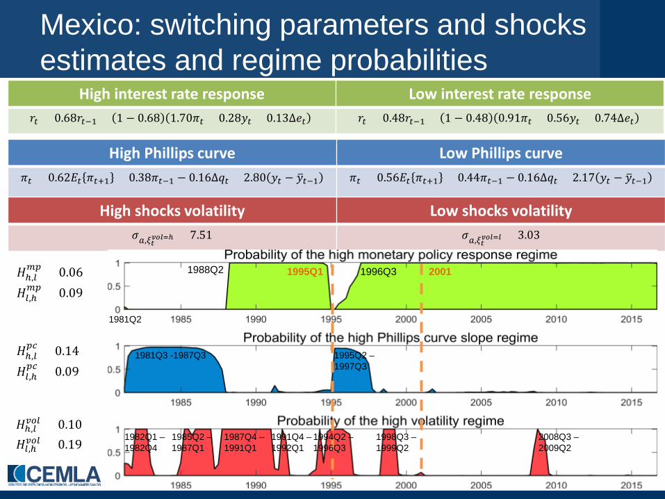
Mexico: switching parameters and shocks estimates and regime probabilities

High interest rate response Low interest rate response 𝑟𝑡 = 0.68𝑟𝑡−1 + 1 − 0.68 1.70𝜋𝑡 + 0.28𝑦𝑡 + 0.13Δ𝑒𝑡 𝑟𝑡 = 0.48𝑟𝑡−1 + 1 − 0.48 0.91𝜋𝑡 + 0.56𝑦𝑡 + 0.74Δ𝑒𝑡

High Phillips curve Low Phillips curve 𝜋𝑡 = 0.62𝐸𝑡 𝜋𝑡+1 + 0.38𝜋𝑡−1 − 0.16Δ𝑞𝑡 + 2.80 𝑦𝑡 − 𝑦�𝑡−1

𝜋𝑡 = 0.56𝐸𝑡 𝜋𝑡+1 + 0.44𝜋𝑡−1 − 0.16Δ𝑞𝑡 + 2.17 𝑦𝑡 − 𝑦�𝑡−1

High shocks volatility Low shocks volatility 𝜎𝑡,𝜉𝑡

𝑣𝑣𝑣=ℎ = 7.51 𝜎𝑡,𝜉𝑡𝑣𝑣𝑣=𝑣 = 3.03

𝐻ℎ,𝑙𝑚𝑝 = 0.06

𝐻𝑙,ℎ𝑚𝑝 = 0.09

𝐻ℎ,𝑙𝑝𝑐 = 0.14

𝐻𝑙,ℎ𝑝𝑐 = 0.09

𝐻ℎ,𝑙𝑣𝑛𝑙 = 0.10

𝐻𝑙,ℎ𝑣𝑛𝑙 = 0.19

1995Q1 2001 1988Q2 1996Q3

1981Q3 -1987Q3 1995Q2 – 1997Q3

1981Q2

2008Q3 – 2009Q2

1998Q3 – 1999Q2

1994Q2 – 1996Q3

1985Q2 – 1987Q1

1987Q4 – 1991Q1

1991Q4 – 1992Q1

1982Q1 – 1982Q4

Mexico: counterfactuals

Output Growth Inflation Interest Rate

M SD M SD M SD

High MP 2.69 4.41 15.26 8.30 23.23 11.38

Low MP 2.97 5.17 29.55 12.29 45.58 31.77

High PC 2.46 4.33 32.38 11.04 55.90 24.04

Low PC 2.42 3.99 11.08 3.89 28.91 9.46

High Vol 2.34 4.71 81.99 27.70 60.41 14.72

Low Vol 2.58 5.08 19.81 10.31 33.71 13.19

Actual 0.00 5.73 21.00 24.78 25.76 26.36

In Mexico, regime switch to H_MP, L_PC and especially L_Vol help to explain the observed reduction of inflation and its volatility without implying higher interest rates, neither lower or more volatile output.