money illusion: a rationale for the tips puzzle - … annual meetings/2018-milan...money illusion: a...

Money Illusion:

A Rationale for the TIPS Puzzle

Abraham Lioui∗ Andrea Tarelli†

April 2018

∗EDHEC Business School, 393 Promenade des Anglais, 06202 Nice Cedex 3, France. Phone: +33 (0)4 93 18 78 68.Fax: + 33 (0)4 93 83 08 10. E-mail: [email protected].

†Catholic University of Milan, Largo A. Gemelli 1, 20123 Milan, Italy. Phone: +39 02 7234 2923. E-mail: [email protected].

Money Illusion:


Abstract

Why is the TIPS market so small? We show that a rational individual, dynamically investing

into multiple asset classes over a 20-year horizon, benefits by 1.2% per annum from having access

to inflation-indexed bonds. However, if the investor suffers from money illusion, the perceived

certainty equivalent gains reduce to less than 0.3%. Furthermore, the benefits become totally

negligible if the money-illusioned investor is less sophisticated and ignores time variations in risk

premia. Money illusion causes significant portfolio shifts from inflation-indexed toward nominal

bonds, with little effects on equity allocations.

JEL classification: E43, E52, G11, G12.

Keywords: Money illusion, Term structure of interest rates, Portfolio choice.

1

1 Introduction

Introduced in the U.S. in 1997, after several periods of high inflation uncertainty, Treasury Inflation-

Protected Securities (TIPS) should have been acclaimed by market participants. They were supposed

to be a close-to-perfect instrument to hedge against inflation and would have offered an observable

measure of the term structure of inflation expectations. Early works in asset allocation strongly

supported the welfare improvement entailed by the inclusion of such securities (Campbell and Viceira,

2001; Brennan and Xia, 2002; Wachter, 2003; Kothari and Shanken, 2004). However, a few years

later, it was obvious that the TIPS market had not delivered in terms of market quality, as the

level of market illiquidity was still noticeably high, especially relative to nominal Treasury Bonds.

Since then, instead of improving, the illiquidity of the TIPS market has persisted, if not deteriorated

(Fleming and Krishnan, 2012). Although the illiquidity does not seem to question the cheapness

of these securities, when compared to other types of debt financing (Campbell and Viceira, 2009),

Figure 1 reveals that the fraction of TIPS with respect to the total of marketable Treasuries was 8.9%

at the end of 2016, and has never been higher than 11% in the last two decades. The situation in other

markets is not very different. For example, at the end of 2016, only 12.3% of the French public debt

and only 12.7% of the Italian public debt was represented by inflation-protected securities. Among

the largest issuers, the only exception seems to be represented by the UK, where inflation-protected

debt has been issued since 1981 and represented 27.3% of the total outstanding debt in 2016.

[Figure 1 about here.]

While substantial progress has been made in identifying the TIPS liquidity premium, few works

have focused on understanding why investors shun this asset class.1 As pointed out in Fleckenstein

et al. (2014), TIPS are typically underpriced with respect to nominal bonds, and the sign of the

1As a matter of fact, none of the inflation-related instruments have encountered the expected success. In additionto TIPS and inflation swaps, CPI-related futures were also introduced in 2004 by the Chicago Mercantile Exchange(CME), but failed to attract investors. Fleming and Sporn (2013) documented a very low trading activity on theinflation swap market, consisting of just over two trades per day on average since 2010.

2

mispricing is consistent with a lack of demand.2

In this paper, we show that money illusion is a potential explanation for a low demand for TIPS.

Money illusion can be described in general terms as a bias in the assessment of the real value of

economic transactions, caused by the fact that people tend to think in nominal amounts.3 The

phenomenon of money illusion has been studied for more than half a century in monetary economics

(Marschak, 1950, 1974; Dusansky and Kalman, 1974), as well as behavioral and experimental eco-

nomics (Shafir et al., 1997; Fehr and Tyran, 2001, 2007, 2014), and has been found to be useful in

solving several asset pricing puzzles.

We look at the distortions on the demand side, and the welfare consequences, brought about

by money illusion in a market where multiple asset classes (nominal and indexed bonds, stocks and

cash) are available. A conservative investor is first considered, who we formally model as an infinitely

risk-averse investor. It is well known (Campbell and Viceira, 2001; Brennan and Xia, 2002) that a

conservative investor, not suffering from money illusion, would allocate all her wealth to an indexed

bond maturing at her investment horizon, or, if not available, would try to replicate it. However,

when money illusion is at play, we find that the investor chooses a combination of indexed and nominal

bonds, for which the relative weights depend on the degree of money illusion. Under extreme money

illusion, all the portfolio is invested in a nominal bond maturing at the investment horizon. Severe

money illusion therefore drives conservative investors out of the indexed bond market. While non-

illusioned investors attempt to hedge future variations of the real rate, conservative money-illusioned

investors partly or completely ignore expected inflation, hedging only variations of the nominal rate.

When investors instead have a moderate risk aversion, the optimal allocation takes also advantage

of the risk/return trade-off offered by indexed and nominal bonds, beyond their capacity to hedge

inflation. We consider both the cases where risk premia are constant and time-varying, discovering

2García and van Rixel (2007) review several arguments for and against the issuance of inflation-indexed bonds fromthe perspective of a central bank, as well as the benefits to investors.

3In this work, money illusion can be either considered as a manifestation of irrationality, which might be the case fora significant fraction of individuals in the economy, or as a rational choice of the agent, which is the case, for example,for fund managers whose compensation is based on nominal returns.

3

that, again, money illusion significantly shifts the portfolio from indexed to nominal bonds. The

impact of money illusion on stock investments is negligible if compared to the effect on optimal

bond positions, as the inflation-hedging properties of both nominal and inflation-indexed bonds are

quantitatively more relevant than for stocks.

A key contribution of our work is that we quantify the economic impact of money illusion under

different perspectives. Firstly, we assess the opportunity cost entailed by money illusion, evaluating

the expected utility loss of a non-illusioned investor who is forced to follow the portfolio strategy of

a partially or totally money-illusioned investor. We find the loss to be substantial, with a certainty

equivalent reduction of about 1% per annum for investment horizons longer than 10 years. This

result is in line with the recent findings by Stephens and Tyran (2016), which were based on Danish

financial and socio-demographic data. Secondly, we provide an explanation for the low market

interest in inflation-protected bonds, by quantifying the opportunity cost, as perceived by both a

non-illusioned investor and by a money-illusioned investor, of removing inflation-indexed bonds from

the investable universe. Consistent with Mkaouar et al. (2017), we find that a non-illusioned investor,

who ignores time variations in risk premia, suffers from a significant utility cost for not having access

to inflation-indexed bonds. The certainty equivalent loss is about 0.5% per annum for a 10-year

investment horizon and 1.25% per annum for a 30-year horizon. However, a money-illusioned investor

perceives a loss inferior to 0.1% per annum when inflation-indexed bonds are not accessible. The

losses are only slightly higher when investors are more sophisticated and account for time variations

in risk premia, but the conclusion is the same: the utility loss suffered by a money-illusioned investor

deprived of the access to inflation-protected instruments is very small, as her perceived expected

utility achievable by substituting real bonds with nominal bonds is almost unchanged. It thus seems

that money-illusioned investors have little incentives to enter the inflation-indexed bond market.

The most general framework we propose is based on a dynamic affine term structure model with

time-varying risk premia, as in Dai and Singleton (2000), Duffee (2002), Joslin et al. (2011), and

4

many others. The model is extended to allow for the pricing of inflation-indexed bonds, partially

inspired by the more recent works by Christensen et al. (2010) and Andreasen et al. (2017). The

term structure model is then applied to an asset allocation problem with multiple asset classes,

as for example in Sangvinatsos and Wachter (2005). We contribute to the literature of dynamic

asset allocation relying on dynamic term structure models, providing a different perspective to the

empirical issues of the sensitivity to estimation errors and the in-sample overfitting of essentially

affine models, as recently pointed out by Duffee (2011), Feldhütter et al. (2012) and Sarno et al.

(2016). In this respect, we implement a simple but effective methodology, aimed at robustifying the

model against the overfitting of time-varying risk premia. This problem typically leads to unrealistic

optimal portfolio positions and largely overstates utility losses entailed by suboptimal strategies,

which we avoid, in the estimation phase, by imposing reasonable bounds to the volatility of the risk

premia in the economy.

As modern economies experienced low inflation rates during the Great Moderation years (80s,

90s) and also since the Great Recession (starting with the financial crisis in 2008), one may wonder

whether the mechanism highlighted in this paper may have been at play in the last decade. Although

regarded as an hyperinflation-related phenomenon, many authors have shown that money illusion

could also be at work in a low-inflation environment. Piazzesi and Schneider (2008) developed an

equilibrium model explaining the house-price booms and stock market undervaluation in both the

1970s and 2000s, which occurred in opposite interest rate and inflation regimes. Brunnermeier and

Julliard (2008) also showed that reductions of inflation may lead to housing bubbles if people suffer

from money illusion. Building on the work by Basak and Yan (2010), David and Veronesi (2013)

developed a general equilibrium model, featuring money illusion, that captures historical stock and

bond co-movements and explains the low P/E ratio and high long-term yields in the late 1970s.

Finally, Miao and Xie (2013) included money illusion in a monetary model of endogenous growth,

showing that the impact of money illusion on long-run growth is already significant when expected

5

inflation is close to its long-run mean. While these contributions highlight the distortions of the

equilibrium introduced by money illusion, our focus is on the individual behavior of an investor with

a long-term finite horizon.

Finally, this work is related to the strand of literature attempting to explain the mispricing and

liquidity puzzles of TIPS. In particular, Fleckenstein et al. (2014) found a massive and persistent

mispricing of TIPS, highlighted by replicating the payoff of nominal Treasury bonds using inflation

swaps and TIPS. They explained this phenomenon invoking the near-money characteristic of nominal

Treasuries4 and justified the persistent nature of the mispricing as an effect of the slow-moving-capital

phenomenon. Christensen and Gillan (2017) provided additional evidence, showing that quantitative

easing reduced the liquidity premium in the TIPS market. Fleming and Sporn (2013) highlighted

the lack of liquidity of inflation swaps and the mispricing of inflation-related securities. The puzzling

illiquidity of TIPS has led several authors to postulate the existence of a systematic liquidity factor,

unique to the TIPS market. The contributions by Pflueger and Viceira (2016), Abrahams et al.

(2016) and Andreasen et al. (2017) proposed several methodologies to extract this factor, finding

evidence that the TIPS risk premium is time-varying and quantitatively significant.

The remainder of the paper is organized as follows. In Section 2, we set up the economic frame-

work and derive the optimal strategy. Section 3 describes the estimation methodology, presents the

dataset and discusses the parameter estimates. In Section 4, we discuss the results of the optimal

portfolio strategy obtained considering constant asset risk premia, at first for a conservative investor,

and then for an investor with a moderate risk aversion. In Section 5, we present additional findings

obtained considering time-varying risk premia. Section 6 concludes the paper. The technical details

and additional empirical findings are relegated to the Appendix.

4See Nagel (2016) on the liquidity premium of near-money assets.

6

2 Optimal portfolio choice

Our long-term investor is allowed to trade nominal and real bonds, a stock index and a nominal

money market account (cash). As usual in asset allocation problems, we are in a situation of partial

equilibrium, whereby the prices of the assets available for trade are given to the investor. We first

describe the economy where the agent trades, and we then derive the optimal portfolio strategy.

2.1 The economy

Stochastic discount factor (SDF) We assume that the nominal SDF dynamics is as follows:

dΦt

Φt= −Rtdt − Λ′

tdzt, (1)

where Rt is the nominal short-term interest rate, and Λt is the n × 1 vector of market prices of the

n systematic risks zt.

Following the literature on dynamic term structure modeling, we assume an affine functional

form for the nominal rate and for the market prices of risk:

Rt = R0 + R′1Xt, (2)

Λt = Λ0 + Λ1Xt, (3)

where R0 is a scalar, R1 an m × 1 vector, Λ0 an m × 1 vector and Λ1 an m × m matrix; finally, Xt is

the m × 1 vector of state variables driving the dynamics of the variables of interest. We assume that

these state variables are persistent and follow an autoregressive process à la Ornstein-Uhlenbeck:

dXt = Θ(

X − Xt

)

dt + Σ′Xdzt, (4)

where Θ is a real m × m mean reversion matrix, X the m × 1 vector of the long-run means of the

7

state variables and ΣX is the n × m volatility matrix.

Nominal quantities are converted into real quantities using the price level, for which the dynamics

is assumed to be as follows:

dPt

Pt= πtdt + σ

′P dzt, (5)

where πt stands for the expected inflation and σP is the n × 1 volatility vector of realized inflation.

As for Rt and Λt, we assume that expected inflation is affine in the state variables:

πt = π0 + π′1Xt, (6)

where π0 is a scalar and π1 an m × 1 vector.

Traded assets We assume that the long-term investor can trade a nominally risk-free asset (cash)

yielding the short-term interest rate Rt. In addition, a stock can be traded and its price, St, is

assumed to have the following dynamics:

dSt

St=(Rt + σ

′SΛt

)dt + σ

′Sdzt, (7)

where σS is the n × 1 volatility vector of the stock.

On the fixed income side, the investor can trade both nominal and real zero-coupon bonds. A

nominal bond delivers one unit of the currency at maturity, while a real bond delivers one unit of

the numeraire. As in Duffie and Kan (1996), nominal discount bond prices are exponentially affine

functions of the state variables. The nominal price of a nominal discount bond with a time-to-

maturity τ is given by:5

B (Xt, τ) = eAN0 (τ)+AN

1 (τ)Xt , (8)

where the scalar AN0 and the 1 × m vector AN

1 solve the system of ODEs given in Appendix A.1.

5See Section A.1 in the Appendix.

8

Applying Itô’s lemma, we can infer the dynamics of the nominal bond price:

dB (Xt, T − t)B (Xt, T − t)

=(

Rt + AN1 Σ′

XΛt

)

dt + AN1 Σ′

Xdzt. (9)

Similarly, the nominal price of a real zero-coupon bond is given by:6

I (Xt, Pt, τ) = PteAI

0(τ)+AI1(τ)Xt , (10)

and its dynamics by:

dI (Xt, Pt, T − t)I (Xt, Pt, T − t)

=(

Rt +(

AI1Σ′

X + σ′P

)

Λt

)

dt +(

AI1Σ′

X + σ′P

)

dzt. (11)

As can be noticed, not only real bond prices span the innovations in the state variables Xt, but also

realized inflation Pt.

To simplify the notation, we denote the nominal price of a generic risky asset at time t by Y it .

Its dynamics takes the following form:

dY it

Y it

=(Rt + σ

′Y iΛt

)dt + σ

′Y idzt. (12)

Preferences Consider a long-term investor endowed with utility from real terminal wealth:

U (wT ) =w

1−γT

1 − γ, (13)

6See Section A.2 in the Appendix.

9

where wT stands for the real wealth at the investor’s horizon T . When the investor is money-

illusioned, we assume that her objective function modifies as follows:

U (wT ) =

(

w1−αT W α

T

)1−γ

1 − γ, (14)

where WT stands for the nominal terminal wealth and 0 ≤ α ≤ 1 measures the degree of money

illusion. When α = 0, the investor is rational, in the sense that she maximizes her expected utility

from real terminal wealth. When α = 1, the investor is completely money-illusioned, as she reasons

only in nominal terms. This specification is inspired by Basak and Yan (2007), Miao and Xie

(2013)and David and Veronesi (2013), although we choose to define utility over terminal wealth

for analytical tractability. In particular, when markets are complete, a quasi-closed-form solution

can also be derived for the case of utility over consumption. However, a specification with utility

over terminal wealth also allows us to obtain analytical results in some relevant cases of suboptimal

portfolio strategies and market incompleteness. These include when the investor follows a strategy

with a different value of α from the value considered as rational, or when the investment universe

includes fewer non-redundant assets than the number of sources of risk in the market.

Given that the relationship between real and nominal wealth is given by wT = WT P −1T , the

objective function becomes:

U (wT ) =

(

w1−αT W α

T

)1−γ

1 − γ=

W1−γT P

−(1−α)(1−γ)T

1 − γ≡ U (WT ) , (15)

with the understanding that the rational case is nested by setting α = 0.

10

Budget constraint Investors allocate their wealth to N risky assets and the money market ac-

count. The dynamics of nominal wealth reads as follows:

dWt

Wt=

N∑

i=1

ωit

dY it

Y it

+

(

1 −N∑

i=1

ωit

)

Rtdt, (16)

where ωit stands for the proportion of (indifferently) real or nominal wealth invested in risky asset i.

Using (12), this dynamics can be written as follows:

dWt

Wt=(Rt + ω

′tΣ

′Λt

)dt + ω

′tΣ

′dzt, (17)

where ωt is the N×1 vector of weights and Σ is a matrix which columns are the volatility vectors of the

risky assets, σY i . The dynamics of real wealth is obtained by applying Itô’s lemma to wt = WtP−1t :

dwt

wt=

(Rt − πt + ω

′tΣ

′ (Λt − σP ) + σ′PσP

)dt +

(ω

′tΣ

′ − σ′P

)dzt.

Market completeness Concerning the estimation of the model, we will see in the next section

that the market is complete, as it is possible to pin down the market prices for all risks introduced

in the economy, and therefore to fully characterize the dynamics of the SDF (1). In order to derive

the optimal portfolio strategy, however, it is important to take into account the issue of market

completeness from the point of view of the investor. The market is complete if there are at least

N = n non-redundant assets available for trade. As we will consider n = 5, we could meet this

conditions, but, in order to obtain results more easily interpretable from the economic point of view,

we prefer to study the optimal allocation considering at most one nominal bond, one inflation-indexed

bond and the stock market, on top of the nominal risk-less asset.7 When utility depends only on

terminal wealth, as is well known since Kim and Omberg (1996), it is possible to solve the optimal

7When several highly correlated bonds are available for trade, optimal unconstrained portfolio positions may reachunrealistically high values, as shown by Sangvinatsos and Wachter (2005).

11

allocation problem even when markets are not complete. In this case, knowing the dynamics of

traded assets does not allow investors to completely span the dynamics of the SDF. To solve this

issue, along the lines of He and Pearson (1991) and Sangvinatsos and Wachter (2005), we write

the market prices of risk Λt as the sum of two components: the first, Λ∗t , corresponding to their

projection onto the returns of the assets available for trade; and the second, νt, orthogonal to the

traded assets. In principle, there exists an infinity of plausible vectors νt. We show in Appendix

B.1 how, among all the possible values of νt, it is possible to impose that the dynamics of optimal

wealth is actually spanned by the traded assets, pinning down the unique vector ν∗t that makes the

optimal wealth achievable with the traded assets. The nominal SDF of the investor is then:

dΦν∗

t

Φν∗

t

= −Rtdt − (Λ∗t + ν

∗t )′ dzt. (18)

Equivalently, it is possible to define a real SDF, denoted as φν∗

t ≡ PtΦν∗

t .

2.2 Optimal portfolio choice under money illusion

Our setting allows us to write a separable value function for the investor’s problem:

J (Wt, t) ≡ max[ωs]Ts=t

Et

[

W1−γT P

−(1−α)(1−γ)T

1 − γ

]

=W

1−γt P

−(1−α)(1−γ)t

1 − γ[F (Xt, t, T )]γ . (19)

The optimal strategy uncovers the typical structure à la Merton:

ωt =1γ

(Σ′Σ

)−1Σ′Λt − (1 − α)

1 − γ

γ

(Σ′Σ

)−1Σ′

σP +(Σ′Σ

)−1Σ′

ΣX

(FX)′

F, (20)

where FX is the column vector of the partial derivatives of F . We show in Appendix B.1 that F

takes the form:

F (Xt, τ) = exp{

12

X′tB3 (τ) Xt + B2 (τ) Xt + B1 (τ)

}

,

12

where B3 (τ), B2 (τ) and B1 (τ) are the solution of a system of Riccati equations.

Taking B3 (τ) = B3(τ)+B′3(τ)

2 , we can rewrite the optimal portfolio strategy (20) as:

ωt =1γ

(Σ

′Σ)−1

Σ′Λt − (1 − α)

1 − γ

γ

(Σ

′Σ)−1

Σ′σP (21)

+(Σ

′Σ)−1

Σ′ΣX

(

B3 (τ) Xt + B′2 (τ)

)

.

The first component is the mean-variance speculative component, taking advantage of the instanta-

neous risk/return trade-off offered by the assets available for trade. The second component hedges

instantaneous realized inflation risk and elicits a direct impact of money illusion. This second term

disappears under severe money illusion (α = 1), which means that the investor is no longer concerned

by realized inflation risk. Risk attached to future inflation does matter for intertemporal hedging

purposes. The last term is the intertemporal hedging component, which is affected by money illu-

sion in a non-linear way. The portfolio strategy is still linear in the state variables (X), driving the

macroeconomic variables (short rate and expected inflation) and the market prices of risk.

To better gather the economics behind the above strategy (20), note that it can be rewritten as:

ωt =1γ

(Σ′Σ

)−1Σ′ [Λt − (1 − α)σP ] + (1 − α)

(Σ′Σ

)−1Σ′

σP (22)

+(Σ′Σ

)−1Σ′

ΣX

(

B3 (τ) Xt + B′2 (τ)

)

.

The investor is interested in the real risk/return trade-off, i.e. the real risk premia traded assets

can offer. As such, for a non-illusioned investor, the first mean-variance component involves the real

market prices of risk Λt − σP , which do indeed represent the volatility of the real SDF. However, in

the presence of money illusion, the investor accounts to a lesser extent for realized inflation volatility,

even ignoring it under severe money illusion (α = 1). The same happens to the second term,

which does not depend on risk aversion: a non-illusioned investor should try to hedge (perfectly

or imperfectly) the inflation risk exposure, but, once again, money illusion distorts this behavior

13

and leads a perfectly illusioned investor to ignore unexpected inflation risk. Overall, money illusion

affects the perception of the risk/return trade-off the investor is subject to, as well as the unexpected

inflation risk to hedge.

What about the intertemporal hedging component? As is well known, this component brings the

horizon effects into the strategy and it is interesting to assess the potential impact of money illusion

on this component. For this purpose, we start looking at the case of an extremely conservative

investor, that is, an investor with an infinite risk aversion. We show in Appendix B.2 that, when the

market prices of risk are constant (Λ1 = 0), the optimal strategy is:

ωγ→∞t = (1 − α)

(Σ

′Σ)−1

Σ′(

ΣXAI1 (τ) + σP

)

+ α(Σ

′Σ)−1

Σ′ΣXAN

1 (τ) . (23)

Remembering that the volatility vector of an indexed bond is ΣXAI1 (τ) + σP and that the

volatility vector of a nominal bond is ΣXAN1 (τ), it is clear that a non-illusioned investor (α = 0)

avoids speculating through the risky assets (bonds and stocks) and invests all the wealth in an

indexed bond, which maturity coincides with the investment horizon. A money-illusioned investor,

conversely, combines an indexed and a nominal bond, both maturing at her investment horizon. The

relative weight of the two is related to the degree of money illusion. An extremely illusioned investor

(α = 1) invests only in a nominal bond with the appropriate maturity.

From the strategy in (23), it appears that realized inflation is ignored by severely money-illusioned

investors. What about expected inflation? As shown in Appendix B.2, the optimal strategy for a

conservative investor can also be written as:

ωγ→∞t = (1 − α)

(Σ

′Σ)−1

Σ′σP +

(Σ

′Σ)−1

Σ′ΣX

[

R′1

(

e−Θτ − I)

Θ−1]′

(24)

− (1 − α)(Σ

′Σ)−1

Σ′ΣX

[

π′1

(

e−Θτ − I)

Θ−1]′

.

It appears that non-illusioned investors, other than hedging unexpected inflation, aim to hedge the

14

real rate, that is, the difference between the nominal rate (loading on the state variables with the

vector R1) and expected inflation (loading on the state variables with the vector π1). Conversely,

money-illusioned investors focus on hedging the short-term nominal rate only, since the two compo-

nents related to realized and expected inflation vanish for α = 1. Clearly, if expected inflation affects

the nominal short-term rate (for example through a monetary policy rule), the illusioned investor

indirectly still partially hedges expected inflation, but expected inflation is not a source of risk which

matters per se.

When risk aversion is finite and risk premia are allowed to be time-varying, there is no immediately

interpretable explicit solution. However, it is worth remembering that:

F (Xt, t, T ) = Et

(

Φν∗

T

Φν∗

t

(PT

Pt

)1−α)1− 1

γ

. (25)

A non-illusioned investor focuses on the quantities driving the real pricing kernel φν∗

t = Φν∗

t Pt, which

are the real rate, unexpected inflation and the market prices of risk. A severely money-illusioned

investor instead focuses on the risks driving the nominal pricing kernel, which are the nominal short-

term interest rate and the market prices of risk. Expected and realized inflation are not relevant to a

money-illusioned investor. In the empirical analysis, we assess the quantitative importance of these

effects.

3 Estimation

In this section, we estimate the model. After describing the dataset used, we present the methodology

employed, highlighting the characteristics of the different specifications for the risk premia that we

consider. Finally, we discuss the estimates of the parameters.

15

3.1 Dataset

We estimate the model using U.S. monthly data from 31st January 1999 until 31st January 2016. We

consider zero-coupon nominal yields for the following maturities: 3 and 6 months, and 1, 2, 3, 5, 7

and 10 years. The 3- and 6-month yields were obtained from the Treasury Bills rates, available on the

Federal Reserve Economic Data website8 (series GS3M and GS6M). The other nominal zero-coupon

yields are the series fitted by Gürkaynak et al. (2007), available on the website of the Federal Reserve

Board.9 We use zero-coupon real yields for the maturities of 5, 7 and 10 years, as fitted in Gürkaynak

et al. (2010), which are also available on the website of the Federal Reserve Board.10 As a broad U.S.

stock market index, we consider the CRSP NYSE/Amex/NASDAQ/ARCA Value-Weighted Market

Index, extracting the end-of-month data from the daily series. To compute realized inflation, we use

the Consumer Price Index for All Urban Consumers: All Items (CPIAUCSL), available at a monthly

frequency on the Federal Reserve Economic Data website.

3.2 Methodology

Along the lines of Joslin et al. (2011), we estimate the model by maximum likelihood, by choosing

as pricing factors the first three principal components of the whole set of the time series of observed

nominal and real yields, which we collect in the vector of state variables Xt.11 We stack the state

variables Xt, the log price index log Pt and the log stock index level log St into a column vector Zt:

Zt =[

X1t X2

t X3t log (St) log (Pt)

]′

, (26)

8https://research.stlouisfed.org/fred2/9https://www.federalreserve.gov/pubs/feds/2006/200628/200628abs.html

10https://www.federalreserve.gov/pubs/feds/2008/200805/200805abs.html11We also tried considering two separate level factors for the nominal and real yields, as in Christensen et al. (2010),

but we did not notice any significant difference in the quality of the estimates, nor in the implications in terms of portfoliochoice. This is probably because of the fact that, differently from their work, we do not impose any constraints on thematrix K1, as we are not interested in obtaining a representation à la Nelson-Siegel of the term structure.

16

for which the dynamics is:

dZt = Bdt + AZtdt + Σ′Zdzt, (27)

where the column vector B and the matrix A can be compactly written as:

B =

ΘX

R0 + σ′SΛ0 − ‖σS‖2

2

π0 − ‖σP ‖2

2

, A =

0 0

−Θ 0 0

0 0

R′1 + σ

′SΛ1 0 0

π′1 0 0

, (28)

where we set X = 0, as the state variables are the principal components of bond yields and are

centered around zero. The volatility matrix ΣZ is obtained by juxtaposing the matrix ΣX and the

vectors σS and σP :

ΣX =

ΣX (1, 1) ΣX (1, 2) ΣX (1, 3)

0 ΣX (2, 2) ΣX (2, 3)

0 0 ΣX (3, 3)

0 0 0

0 0 0

, σP =

σP (1)

σP (2)

σP (3)

σP (4)

0

, σS =

σS (1)

σS (2)

σS (3)

σS (4)

σS (5)

.

Applying a Euler scheme, we perform an exact discretization of this joint continuous-time process,

which constitutes the first contribution to the log-likelihood function.12 The second contribution to

the likelihood function is obtained by imposing the bond pricing restrictions, which relate the current

value of the state variables Xt to the observed nominal and real bond yields. We allow for Gaussian

observation errors, uncorrelated both in time series and cross-sectionally, with a constant standard

deviation σBε for the nominal yields and σI

ε for the real yields.

We numerically maximize the likelihood function with respect to the whole set of model parame-

12For details on the exact discretization of the continuous-time process and on the construction of the likelihoodfunction, refer to Sangvinatsos and Wachter (2005) or Koijen et al. (2010).

17

ters at the same time, by considering different alternatives to the restrictions that can be imposed on

the time-varying market prices of risk. Firstly, we consider a specification with the restriction that

the asset risk premia are constant, which we obtain imposing that Λ1 = 0. Secondly, we consider

a specification with time-varying risk premia, initially with no restrictions imposed on the matrix

Λ1. As in Christensen et al. (2010), we then iterate the estimation, by progressively imposing a zero

restriction on the element of Λ1 with the lowest t-statistics, stopping when all the elements of Λ1

have a t-stat higher than 2.13 Thirdly, we consider a specification where we let the risk premia of

the risky assets vary, but constraining their volatility to some reasonable values. In particular, we

impose that the volatility of the risk premia of the nominal bonds,∥∥∥AN

1 Σ′X

Λ1Σ′X

∥∥∥, and the real

bonds,∥∥∥

(

AI1Σ′

X+ σ

′P

)

Λ1Σ′X

∥∥∥, are not higher than the volatility of the short-term interest rate,

which is equal to 0.64% per annum.14 We also impose that the volatility of the risk premium of

realized inflation, ‖σ′P Λ1Σ′

X‖, is not higher than 0.5% per annum and, finally, that the volatility

of the equity premium, ‖σ′SΛ1Σ′

X‖, is not higher than 1% per annum. By imposing economically

reasonable restrictions on the time variation of risk premia, this methodology attempts to implement,

as suggested by Sarno et al. (2016), a modeling approach that is flexible but limits overfitting.

For the empirical study, we consider as base case the results obtained for constant risk premia,

which is for our purpose the most reliable framework, allowing us to focus on the roles of interest rate,

expected inflation and realized inflation hedging. We also present the results obtained for the case

of volatility-constrained time-varying risk premia. We relegate to the Appendix the results obtained

in the case where the statistically significant elements of Λ1 are left unconstrained, justifying why

we deem that this framework is not appropriate for the analysis.

13Similar procedures have been followed by several authors, such as Duffee (2002), Sangvinatsos and Wachter (2005)and Christensen et al. (2010). Joslin et al. (2014) performed a model selection among all possible sets of zero restrictionson the elements of Λ1. This would entail very long computation times in our continuous-time framework.

14We choose to impose this restriction for the 3- and 10-year nominal bonds, and for the 7-year real bond.

18

3.3 Parameter estimates

Table 1 shows the parameter estimates for the specification with constant risk premia (Panel (a))

and with volatility-constrained risk premia (Panel (b)). The estimates of the parameters related

to the instantaneous nominal risk-free rate, R0 and R1, are, as expected, almost identical in the

two settings, as well as the volatility vectors and the vector of constant risk premia Λ0. R0 is very

close to the average 3-month nominal yield (1.85% vs 1.87%). π0 represents the drift of the price

index under the historical probability measure and is similar between the two settings, being equal

to about 2.10%. The average of the instantaneous real rate is given by R0 − π0 + σ′PΛ0 = 0.92%.

The vector of loadings π1 is different between the two settings, but we verified that, as expected,

the corresponding quantities under the pricing measure, π1 − Λ′1σP , are almost identical. The

same applies to the mean-reversion matrices, Θ, which are different between the two settings, but

the quantities Θ + Σ′XΛ1 are equal to each other. Finally, the standard deviations of the pricing

errors relative to the nominal yields, σBǫ , are in both settings equal to 12 basis points, while the

corresponding quantities for real yields, σIǫ , are both equal to 7 basis points.

[Table 1 about here.]

The goodness of fit relative to the historical distributions can be checked in Table 2, where

we report the annualized mean values and the volatilities, both historical and model-implied, of

bond yields, realized inflation and realized equity returns. The two specifications fit the historical

moments very well. The model-implied means of the risk premia are also very similar in the two

settings. The fitted risk premia of the nominal bonds are about 0.3% − 0.5% higher than the risk

premia of inflation-indexed bonds for the same maturities. The realized inflation risk premium is

definitely non-negligible and about 1.2% in both settings, while the equity premium is just below

5%. The risk premia volatilities for the second setting are close to the bounds imposed, i.e. the bond

premia volatilities are close to the volatility of the historical 3-month rate (0.64%), while the realized

inflation and equity risk premium volatilities are respectively 0.5% and 1%. Finally, the short-rate

19

volatilities are similar between the two settings, while the model-implied volatility of the expected

inflation is slightly higher when the risk premia are time-varying.


Table 3 shows, whenever available, the pairwise correlations between returns and economic vari-

ables, both from the historical distribution and as implied by the estimated parameters for the two

specifications. The model-implied pairwise correlations are rather similar to each other and fit the

historical values reasonably well, with some exceptions among the correlations involving short-term

nominal yields. Real bond returns, differing from nominal bond returns, are positively correlated

with the price index. They also have a weak correlation with equity returns, while nominal bond

returns are negatively correlated with the equity. Nominal and real bond returns corresponding to

the same maturities tend to be strongly positively correlated. Furthermore, it is interesting to look

at the model-implied correlations between asset returns and the unobservable economic variables.

Nominal bond returns seem to be more (negatively) correlated with the short-term rate R w.r.t. real

bond returns for the same maturities. Real bond returns, differing from nominal bond returns, are

strongly positively correlated with the innovations in the expected inflation π and strongly negatively

correlated with the real rate r.


The first row of graphs in Figure 2 shows, for the two specifications, the model-implied short-term

interest rate, the expected inflation, the break-even inflation and the Blue Chip inflation forecast.

The expected inflation is slightly higher than the break-even inflation, and the difference between

the two is the realized inflation risk premium. The expected inflation is overall in line with the

Blue Chip forecast in both cases. The second row of graphs represents the risk premia of a 10-

year nominal bond, a 10-year real bond, the stock and the realized inflation. In the model with

time-varying volatility-constrained premia, these are centered around the values for the constant risk

20

premia specification, and their ranges of variation seem to be reasonable, going from about 2% to 5%

for the two 10-year bonds, from −2% to 9% for the stock and from about 0% to 2% for the realized

inflation premium. The third row of graphs show the myopic allocation followed by a mean-variance

investor with a risk aversion γ = 10. When risk premia are time-varying, these positions also vary

with time. As can be noticed, the positions range from −50% to about 100%, without reaching

excessive levels of leverage or short selling, as expected by an investor with a moderate level of risk

aversion. The fourth row shows the maximum ex-ante Sharpe ratio achievable with the three assets

above, which is about 0.6 for the specification with constant risk premia, and ranges between 0.4

and 1 for the model with time-varying risk premia.


Figure A.3 in Appendix D.1 shows the same time series as Figure 2 for the specification with

time-varying risk premia and no volatility constraints. The time series of risk premia, the mean-

variance portfolio weights and the maximum achievable Sharpe ratio are subject to variations which

are unreasonably large.15 These quantities are indeed not directly observable, and a model that

over-fits in-sample data has the drawback of returning uncontrollably volatile time series for these

unobservable quantities.

For our empirical analysis, we choose to use as base case the model with constant risk premia

and to verify that the results are consistent with those obtained considering the specification with

volatility-constrained risk premia. We discuss in Appendix D why, although qualitatively confirming

most of our empirical results, we do not deem the specification with volatility-unconstrained risk

premia to be reliable for our analysis. Our choice is consistent with the findings of Feldhütter et al.

(2012) and Sarno et al. (2016), who argued that (unconstrained) essentially affine term structure

models are very sensitive to estimation errors and in-sample overfitting. We also take into account the

in-sample empirical results of Sangvinatsos and Wachter (2005) and Barillas (2011), who found very15Duffee (2011) noticed the same empirical fact and attempted to reduce the issue of estimation overfitting by

imposing a numerical constraint on the average value of the maximum achievable Sharpe ratio.

21

large portfolio positions and unrealistically high utility losses associated with suboptimal portfolio

strategies.16

4 Main empirical findings

We start our empirical investigation considering the case where risk premia are constant. We have

already argued that this is a robust setting in an asset allocation context, being less prone to over-

fitting than models with time-varying premia and, as pointed out by Feldhütter et al. (2012), less

sensitive to estimation errors. Furthermore, in this context, we can unambiguously associate the

intertemporal hedging demands, and their variations corresponding to different degrees of money

illusion, to the economic variables, such as the short-term rate, the expected inflation and the real

rate. We first consider a conservative investor, that is, an individual with an infinite risk aversion,

and we then extend the analysis to the case of a moderate investor, that is, an individual with a

medium level of risk aversion (γ = 10).

4.1 Conservative investor

Portfolio strategy In the case of γ → ∞ and constant risk premia it is possible to explicitly

determine the optimal portfolio strategy, as in (23). Figure 3 reports the positions in the four assets

for different degrees of money illusion. α = 0 corresponds to a non-illusioned investor, α = 0.5 to

a partially illusioned investor and α = 1 to a totally money-illusioned investor. The state variables

are at their long-run means.


A conservative investor with a very short horizon invests only in the money market account

(cash). Increasing the horizon leads to an investment in the other assets. A particular case arises16To the best of our knowledge, only Duffee (2002) documented an acceptable out-of-sample predictive ability of

unconstrained essentially affine term structure models. This analysis, however, is based on rather small sample (lessthan 4 years of out-of-sample monthly observations). Duffee (2002) also found a suspiciously high in-sample model-implied volatility of bond risk premia.

22

when the horizon equals 10 years, that is the maturity of the bonds available for trade. A rational

investor (α = 0) allocates all wealth in the indexed bond and nothing in the other assets. For

intermediate levels of money illusion, the investor reduces the position in the real bond and increases

the position in the nominal bond. A severely money-illusioned investor (α = 1) invests only in the

nominal bond. For any investment horizon, the stock and the cash positions are barely affected by

the degree of money illusion.

In terms of intertemporal hedging demands, an interesting pattern appears: while the position

in the nominal bond flattens when the investment horizon is above 10 years, the position in the real

bond keeps increasing steadily. Roughly, a rational investor allocates 0% in the nominal bond if the

investment horizon is 10 years and about 20% when the horizon is 20 or 30 years. The corresponding

figures for the position in the indexed bond are 100%, 150% and 170%, respectively. This is a direct

consequence of the dynamics of expected inflation, which loads more than the nominal short-term

rate on the less persistent state variables driving the economy (X2 and X3).

The stock position for a conservative investor is very small, it is almost not sensitive to money

illusion and, as expected, is increasing in the investment horizon. It is equal to zero when the latter

is equal to 10 years, i.e. the maturity of the bonds. The cash position decreases from 100% for short

horizons to zero when the horizon is equal to 10 years, when the portfolio is fully invested in bonds.

The cash position keeps decreasing toward negative values, implying leveraged positions in the other

assets, for horizons longer than 10 years.

While money illusion strongly shifts the portfolio from indexed to nominal bonds, the indexed

bond position is zero only when the nominal bond maturity is equal to the investment horizon and

money illusion is severe. Overall, given that nominal bonds for almost any maturity up to 30 years

exist, we can confidently say that money illusion drives conservative investors away from the indexed

bond market, as a conservative money-illusioned investor allocates all wealth into a nominal bond

maturing at her investment horizon. Conversely, if indexed bonds were available for all maturities,

23

conservative non-illusioned investors would invest only in indexed bonds.

Intertemporal hedging demands It is evident that the intertemporal hedging components (hori-

zon effects) of the optimal portfolio strategy in Figure 3 are substantial, and money illusion causes

a shift from the indexed to the nominal bond market. Given that market prices of risk are constant

so far, is this related to expected inflation or the nominal short-term rate? In Figure 4, we show

the projections of the intertemporal hedging components of each asset position onto the expected

inflation and the nominal short-term rate, as well as the corresponding orthogonal components.


As can be noticed, the component of intertemporal hedging projected onto expected inflation

is substantial and very sensitive to the degree of money illusion, while the orthogonal component

is far less sensitive. The mechanism at play is straightforward: investors take long positions on

indexed bonds and short nominal bonds in order to hedge expected inflation. Money illusion tends

to decrease (in absolute value) these positions. The intertemporal hedging demand corresponding

to the stock is mostly correlated to expected inflation and, as stock returns are positively correlated

with the expected inflation π (see Table 3b), the hedging demand is decreasing with α. However, as

the inflation-indexed bond has better inflation-hedging properties, the stock position is very small.

The two bottom rows of Figure 4 deliver a totally different picture, as the intertemporal hedging

activity projected onto the nominal short-term rate is negligible, and the sensitivity to α is also

very small. One may be surprised that, even for a money-illusioned investor, the projection of the

hedging demand onto the nominal risk-free rate is small. This is due to the low correlation between

the short-term rate and the 10-year nominal and real bonds, as documented in Table 3.

In short, when risk premia are constant, the intertemporal hedging activity for a conservative

investor is linked to the rationale of hedging expected inflation, while the nominal interest rate plays

a marginal role. Money illusion tends to reduce the demand for assets hedging dynamic variations

24

of expected inflation. When both types of bonds are available, they are used to perform most of the

intertemporal hedging activity, while the stock plays a marginal role.

Impact of money illusion on equity investments In order to further investigate the impact of

money illusion on stock positions, we show in Figure 5 the portfolio strategy of rational and illusioned

investors when one of the bonds (either nominal or real) is removed from the asset universe.


Figure 5a represents a situation where the investor does not have access to the inflation-indexed

bond market, which is nowadays a realistic situation in many financial markets. The nominal bond

position is increasing in the investment horizon, while we saw in Figure 3 that it flattens when

indexed bonds are available, and is essentially insensitive to money illusion. The stock position

tends to increase with the horizon and is substantial (respectively 10% and 20% for a 10- and a

20-year horizon) for a non-illusioned investor, as the stock is used to hedge expected inflation in

spite of the real bond. The stock position is instead substantially reduced when the degree of money

illusion is higher.

Figure 5b shows that, when only indexed bonds are available (which is not a realistic situation in

current fixed-income markets), their position is monotonically increasing in the investment horizon

and decreases with the degree of money illusion. Furthermore, this long position is partially offset

by a negative stock position when the degree of money illusion is high, while the stock position is

virtually zero for a non-illusioned investor, who benefits from the inflation-hedging properties of the

real bond.

Synthesis A conservative money-illusioned investor shuns the stock market and takes small posi-

tions in the indexed bond. The impact of money illusion is substantial, as it drives investors out of

the indexed bond market toward the nominal bond market.

25

4.2 Moderate investor

Consider now a moderate investor, with risk aversion of γ = 10. For this investor, the risk/return

trade-off offered by the opportunity set plays a role also through the speculative component, which is

represented by the first term in (22). We want to assess the impact of money illusion in this context

and see how the optimal portfolio strategy is similar and how it differs from the results obtained for

the infinitely risk-averse investor. Furthermore, as risk aversion is finite, we are able to calculate an

annualized certainty equivalent for the investment and to make welfare considerations.

Portfolio strategy The portfolio strategy shown in Figure 6 mimics the pattern observed for the

conservative investor, although with respect to the case of γ → ∞, the optimal positions are offset, as

the first speculative component of (22) is nonzero. A rational investor with a 10-year horizon invests

60% in the nominal bond, rather than 0% as the conservative investor. Conversely, the position in the

indexed bond is around 80%, rather than 100%. In spite of these differences, money illusion affects

the portfolio strategy similarly to the case of a conservative investor, as it entails a reduction of the

optimal position in the real bond and an increase of the position in the nominal bond. Furthermore,

the amount of this substitution effect is similar to that observed in Figure 3. As expected, the stock

position is higher compared to the case of a conservative investor, but the optimal position is again

almost insensitive to money illusion.


Utility loss due to money illusion Of particular interest is the welfare cost of money illusion.

We estimate it considering the portfolio strategy followed by an agent with a degree of money

illusion α and calculate the expected utility perceived by a non-illusioned investor forced to follow

that strategy. The cost is expressed in terms of annualized certainty equivalent loss. The derivation

of the value function for an investor following a strategy suboptimal for her preferences is detailed

in Appendix B.3, while in Appendix B.4 we describe how we compute the loss.

26

The opportunity cost ℓann, for different degrees of money illusion α, is shown in the bottom

graph of Figure 6. As expected, the annualized loss increases with α, but not linearly, as for a

10-year horizon and α = 0.5, we observe an annualized loss of 0.25%, while for a totally illusioned

agent (α = 1), the loss is almost 1% per annum. Furthermore, the annualized loss steeply increases

with the investment horizon up to around 10 years, and keeps increasing at a lower rate when the

horizon is longer. For α = 1 and a 30-year horizon, the annualized loss is about 1.2%.

Overall, it seems that, when all the investable assets we consider are available for dynamic

trading, the opportunity cost of money illusion is substantial. Our estimate is totally consistent with

the findings of Stephens and Tyran (2016), who estimated that 10-year portfolio returns were about

10 percentage points lower for Danish money-illusioned individuals.

Perceived utility loss due to the unavailability of inflation-indexed bonds for different

degrees of money illusion Figure 7a shows the optimal portfolio strategy when the investor has

no access to inflation-indexed bonds. The effect of an increasing degree of money illusion on the

portfolio weights is comparable to that already noted for the conservative investor, with little effect

on the nominal bond position and a reduction in the stock position.


The most interesting result is shown, however, in the bottom-right panel of Figure 7a, where

the annualized certainty equivalent loss due to the exclusion of the inflation-indexed bond from

the investable universe is shown. The opportunity cost of not having access to the real bond is

increasing in the investment horizon and is substantial for a non-illusioned investor (α = 0), being

equal to 1.25% per annum for a 30-year horizon. However, the opportunity cost of removing the

inflation-indexed bond is perceived as negligible by a totally money-illusioned investor (α = 1).

It is crucial that, for an illusioned agent, the utility cost of not having access to inflation-indexed

bonds is negligible. This may represent an explanation for the low market demand for inflation-

27

protected securities. Although the optimal portfolio weight associated with the inflation-indexed

bond may not be exactly zero, because of the fact that an illusioned investor perceives a negligible

loss for not investing in inflation-protected securities, her demand for this kind of securities is likely

to be low, as they can be effectively substituted by more traditional assets, such as nominal bonds

and stocks.

Figure 7b refers to the opposite situation, showing the optimal portfolio strategy and certainty

equivalent loss of an investor deprived of the access to nominal bonds. This situation is highly

hypothetical, given the enormous size of the nominal bond market, but it is useful to completely

grasp the intuition obtained from the previous analysis. The results are complementary to those

obtained in the panel above: there is very little effect in terms of portfolio allocation in the inflation-

indexed bond, while a money-illusioned investor tends to allocate a smaller fraction of wealth into

the stock market. In terms of the opportunity cost of removing nominal bonds from the investable

universe, a money-illusioned investor is severely hurt, while a non-illusioned investor, who tends to

favor the allocation into inflation-indexed bonds, is significantly less affected.

Synthesis It seems that money illusion significantly affects the optimal portfolio strategy of long-

term investors, and in particular the positions taken in nominal and inflation-indexed bonds. The

utility cost of money illusion, if evaluated from the point of view of a fully rational and non-illusioned

investor, is significant. Although the optimal allocation of a money-illusioned investor also comprises

an investment in inflation-indexed bonds, we show that by excluding inflation-indexed bonds from the

investable universe, the utility loss perceived by an illusioned investor is very small, as her perceived

expected utility substituting real bonds with nominal bonds is almost unchanged. In Appendix C,

we prove that these results are robust to variations of the realized inflation risk premium, which is

a quantity which previous studies have shown to be difficult to estimate.

28

5 Additional empirical findings: time-varying risk premia

In this section, we present additional empirical results, which support the evidence obtained in the

previous section for the setting where risk premia are constant, by considering a setting where risk

premia are allowed to be time-varying. We focus on the case of the moderate investor (γ = 10),

considering the specification where risk premia are time-varying and their volatilities have been

constrained, as specified in Section 3.3. The parameter estimates used are those in Table 1b. We

relegate to Appendix D the analysis based on the specification with time-varying risk premia without

any volatility constraint. The analysis confirms the conclusions we draw in this section, by provid-

ing qualitatively compatible results, but it unrealistically overstates the optimal dynamic portfolio

positions and the certainty equivalent returns, facts for which we provide an explanation.

Portfolio strategy Figure 8 shows the optimal portfolio strategy when investors have access to

the full investment universe. For short investment horizons, the optimal strategy is virtually identical

to the case where risk premia are constant (Figure 6). When the horizon is increased beyond 5 years,

the impact of time-varying risk premia seems to shift the optimal portfolio from nominal bonds to

inflation-indexed bonds. For a 30-year horizon, the increase of the weight in the real bond is between

30% and 50%, corresponding to an approximately equivalent reduction of the weight in the nominal

bond. This is true for any value of α, which suggests that there is little interaction between money

illusion and the intertemporal hedging demands arising from capturing the time variation in risk

premia.


Utility loss due to money illusion The welfare analysis in the graph at the bottom of Figure 8,

showing the certainty equivalent loss attributable to money illusion, confirms that the welfare effect

of money illusion is substantial. The loss is very similar in pattern and size to the case of constant

29

risk premia. In fact, the annualized loss is about 1% for a totally illusioned investor with a 10-year

horizon w.r.t. a rational investor.17


degrees of money illusion We consider now the case where one of the bonds is removed from

the investable universe. Figure 9a shows the case where the inflation-indexed bond is unavailable.

In terms of portfolio positions, qualitatively, the effect of money illusion on the optimal allocation

is similar to the case with constant risk premia (Figure 7a), although in this case, the effect of

money illusion on the intertemporal hedging component associated with the nominal bond is more

pronounced, leading to a position for the illusioned investor which is higher by 30% to 40% for a

horizon longer than 10 years w.r.t. the non-illusioned investor. This difference corresponds to a

different degree of leverage, as reflected by the cash position.


The evaluation of the opportunity cost, perceived by investors with different levels of α, of

excluding the real bond, is crucial to confirm that a money-illusioned investor does not perceive

as useful the availability of inflation-protected securities. Indeed, in this situation, other than for

inflation hedging, an investor who times the market also takes positions in the assets to also hedge

future variations in the risk premia. As can be noticed in Figure 9a, the opportunity cost is substantial

for the fully rational investor (α = 0). The annualized loss increases steadily with the investment

horizon, being equal to 0.5% per annum for a 10-year horizon, 1.1% for a 20-year horizon and 1.7% for

a 30-year horizon. However, considering a partially illusioned investor (α = 0.5), the perceived loss is

already significantly reduced, reaching a maximum of 1% for a 30-year horizon. A totally illusioned

investor (α = 1) perceives a significantly lower loss, which is roughly flat and equal to 0.25% per

17Our analysis is focused on relative losses, not on the absolute value of certainty equivalent returns, which is ex-ante

higher when accommodating time-varying risk premia. We verify that, for investment horizons beyond 5 years, ourspecification of time-varying premia entails a certainty equivalent gain of around 0.2% per annum w.r.t. the case ofconstant risk premia.

30

annum up to a 20-year horizon, and increasing to a maximum of 0.6% for a 30-year horizon.

Finally, for the sake of completeness, we show in Figure 9b the complementary case, where the

nominal bond is excluded from the investable universe. The highest utility loss is sustained by

the illusioned investor (about 1.5% per annum for a 10- to 30-year horizon), while a non-illusioned

investor perceives a loss equal to about 0.4% per annum.

In conclusion, our analysis confirms that a money-illusioned investor, even when attempting to

time the market by accounting for time-varying premia, perceives a significantly lower opportunity

cost of not having access to inflation-indexed instruments than a non-illusioned investor. Among the

money-illusioned investors, even those following sophisticated dynamic strategies seem to be able to

attain comparable expected utilities by substituting inflation-indexed bonds with more traditional

assets, such as nominal bonds and stocks, and therefore have few incentives to enter the inflation-

indexed bond market.

6 Conclusions

Several authors have studied the effects of money illusion on financial markets. Modigliani and Cohn

(1979) recognized money illusion as the source of major errors in the evaluation of common stocks

during periods of anticipated hyperinflation, concluding that these evaluation mistakes were the main

cause of a 50% undervaluation of U.S. stock value at the end of 1977. Their analysis was confirmed by

Cohen et al. (2005), who tested the effects of money illusion in a CAPM-based framework, identifying

an irrational increase of expected returns across all stocks, irrespective of the riskiness (beta) of the

stock, during periods of hyperinflation. More recently, Schmeling and Schrimpf (2011) found that

survey-based measures of expected inflation are able to predict aggregate stock returns, attributing

this phenomenon to money illusion.

The present work shows that the mechanism at play in the aforementioned empirical investigations

is also crucial for the decision-making of a long-term investor. Our results confirm some of the findings

31

of Stephens and Tyran (2016), who documented a tendency for money-illusioned investors to shift

portfolios toward nominal assets. In particular, an illusioned investor tends to reduce the allocation

in inflation-indexed bonds, which intertemporally hedges expected inflation, in favor of nominal

bonds. The effect on the stock allocation is marginal. We estimate the cost of money illusion to

be around 1% per annum for a moderately risk-averse individual with an investment horizon of 10

years or longer. Our findings do not suffer from the cognitive challenge of experiments aimed at

identifying money illusion, as stated by Petersen et al. (2011). We estimate that a fully rational

non-illusioned investor suffers from a utility loss that ranges from about 0.5% to 1.5% per annum for

investment horizons of between 10 to 30 years. Conversely, the perceived welfare loss of a money-

illusioned investor who has no access to inflation-indexed bond is, depending on the specification of

the risk premia considered, negligible or significantly lower. This finding identifies money illusion

as potentially being at the origin of the scarce demand for TIPS in the market, as money-illusioned

investors understate the utility loss entailed by substituting inflation-indexed bonds with nominal

bonds.

From the technical standpoint, we have contributed to the literature of dynamic asset allocation

relying on dynamic affine term structure models, showing some other aspects of the empirical issues

of essentially affine models that have recently been pointed out by Feldhütter et al. (2012) and

Sarno et al. (2016). In particular, we implement a simple, but effective, methodology, to reduce the

problem of the in-sample overfitting of the risk premia, which typically leads to unrealistic optimal

portfolio positions and largely overstates utility losses entailed by suboptimal strategies. The use of

this methodology entails the choice of bounds to the volatility of the risk premia in the economy,

which we impose by choosing some values dictated by common sense. We leave for future research a

formal analysis of this methodology, which would allow a more accurate fine tuning of the restrictions

to be imposed in the estimation phase.

32

References

Abrahams, M., T. Adrian, R. K. Crump, E. Moench, and R. Yu (2016). Decomposing real andnominal yield curves. Journal of Monetary Economics 84 (C), 182–200.

Andreasen, M. M., J. H. Christensen, S. Riddell, et al. (2017). The TIPS liquidity premium.Manuscript, Federal Reserve Bank of San Francisco.

Barillas, F. (2011). Can we exploit predictability in bond markets? Working paper.

Basak, S. and H. Yan (2007). Equilibrium asset prices and investor behavior in the presence of moneyillusion: A preference-based formulation. In EFA Meetings, WFA Meetings.

Basak, S. and H. Yan (2010). Equilibrium asset prices and investor behaviour in the presence ofmoney illusion. The Review of Economic Studies 77 (3), 914–936.

Brennan, M. and Y. Xia (2002). Dynamic asset allocation under inflation. The Journal of Fi-

nance 57 (3), 1201–1238.

Brunnermeier, M. K. and C. Julliard (2008). Money illusion and housing frenzies. The Review of

Financial Studies 21 (1), 135–180.

Campbell, J. and L. Viceira (2001). Who should buy long-term bonds? American Economic

Review 91 (1), 99–127.

Campbell, J. and L. Viceira (2009). Understanding inflation-indexed bond markets. Brookings Papers

on Economic Activity Spring, 79–120.

Christensen, J. H. and J. M. Gillan (2017). Does quantitative easing affect market liquidity? FederalReserve Bank of San Francisco.

Christensen, J. H., J. A. Lopez, and G. D. Rudebusch (2010). Inflation expectations and riskpremiums in an arbitrage-free model of nominal and real bond yields. Journal of Money, Credit

and Banking 42 (s1), 143–178.

Cohen, R. B., C. Polk, and T. Vuolteenaho (2005). Money illusion in the stock market: TheModigliani-Cohn hypothesis. The Quarterly Journal of Economics 120 (2), 639–668.

Dai, Q. and K. J. Singleton (2000). Specification analysis of affine term structure models. The

Journal of Finance 55 (5), 1943–1978.

David, A. and P. Veronesi (2013). What ties return volatilities to price valuations and fundamentals?Journal of Political Economy 121 (4), 682–746.

Duffee, G. R. (2002). Term premia and interest rate forecasts in affine models. The Journal of

Finance 57 (1), 405–443.

Duffee, G. R. (2011). Sharpe ratios in term structure models. Working papers, the Johns HopkinsUniversity, Department of Economics.

Duffie, D. and R. Kan (1996). A yield-factor model of interest rates. Mathematical Finance 6 (4),379–406.

33

Dusansky, R. and P. J. Kalman (1974). The foundations of money illusion in a neoclassical micro-monetary model. American Economic Review 64 (1), 115–122.

Fehr, E. and J.-R. Tyran (2001). Does money illusion matter? American Economic Review 91 (5),1239–1262.

Fehr, E. and J.-R. Tyran (2007). Money illusion and coordination failure. Games and Economic

Behavior 58 (2), 246–268.

Fehr, E. and J.-R. Tyran (2014). Does money illusion matter?: Reply. The American Economic

Review 104 (3), 1063–1071.

Feldhütter, P., L. S. Larsen, C. Munk, and A. B. Trolle (2012). Keep it simple: Dynamic bondportfolios under parameter uncertainty. Working paper.

Fleckenstein, M., F. A. Longstaff, and H. Lustig (2014). The TIPS-Treasury bond puzzle. The

Journal of Finance 69 (5), 2151–2197.

Fleming, M. J. and N. Krishnan (2012). The microstructure of the TIPS market. Federal Reserve

Bank of New York, Economic Policy Review 18, 27–45.

Fleming, M. J. and J. Sporn (2013). Trading activity and price transparency in the inflation swapmarket. Federal Reserve Bank of New York, Economic Policy Review 19, 45–57.

García, J. Á. and A. van Rixel (2007). Inflation-linked bonds from a central bank perspective.Documentos ocasionales-Banco de España (5), 9–47.

Gürkaynak, R., B. Sack, and J. Wright (2007). The US Treasury yield curve: 1961 to the present.Journal of Monetary Economics 54 (8), 2291–2304.

Gürkaynak, R. S., B. Sack, and J. H. Wright (2010). The TIPS yield curve and inflation compensa-tion. American Economic Journal: Macroeconomics 2 (1), 70–92.

He, H. and N. D. Pearson (1991). Consumption and portfolio policies with incomplete markets andshort-sale constraints: The infinite dimensional case. Journal of Economic Theory 54 (2), 259–304.

Joslin, S., M. Priebsch, and K. Singleton (2014). Risk premiums in dynamic term structure modelswith unspanned macro risks. The Journal of Finance 69 (3), 1197–1233.

Joslin, S., K. J. Singleton, and H. Zhu (2011). A new perspective on Gaussian dynamic term structuremodels. The Review of Financial Studies 24 (3), 926–970.

Kim, T. S. and E. Omberg (1996). Dynamic nonmyopic portfolio behavior. The Review of Financial

Studies 9 (1), 141–161.

Koijen, R. S., T. E. Nijman, and B. J. Werker (2010). When can life cycle investors benefit fromtime-varying bond risk premia? The Review of Financial Studies 23 (2), 741–780.

Kothari, S. and J. Shanken (2004). Asset allocation with inflation-protected bonds. Financial

Analysts Journal 60 (1), 54–70.

Marschak, J. (1950). The rationale of the demand for money and of “money illusion”. Metroeconom-

ica 2 (2), 71–100.

34

Marschak, J. (1974). Money illusion and demand analysis. In Economic Information, Decision, and

Prediction, pp. 206–221. Springer.

Miao, J. and D. Xie (2013). Economic growth under money illusion. Journal of Economic Dynamics

and Control 37 (1), 84–103.

Mkaouar, F., J.-L. Prigent, and I. Abid (2017). Long-term investment with stochastic interest andinflation rates: The need for inflation-indexed bonds. Economic Modelling.

Modigliani, F. and R. A. Cohn (1979). Inflation, rational valuation and the market. Financial

Analysts Journal 35 (2), 24–44.

Nagel, S. (2016). The liquidity premium of near-money assets. The Quarterly Journal of Eco-

nomics 131 (4), 1927–1971.

Petersen, L., A. Winn, et al. (2011). The role of money illusion in nominal price adjustment. American

Economic Review, 1–26.

Pflueger, C. E. and L. M. Viceira (2016). Return predictability in the treasury market: Real rates,inflation, and liquidity. In Handbook of Fixed-Income Securities, pp. 191–209. Wiley Online Library.

Piazzesi, M. and M. Schneider (2008). Inflation illusion, credit, and asset prices. In Asset prices and

monetary policy, pp. 147–189. University of Chicago Press.

Sangvinatsos, A. and J. A. Wachter (2005). Does the failure of the expectations hypothesis matterfor long-term investors? The Journal of Finance 60 (1), 179–230.

Sarno, L., P. Schneider, and C. Wagner (2016). The economic value of predicting bond risk premia.Journal of Empirical Finance 37 (C), 247–267.

Schmeling, M. and A. Schrimpf (2011). Expected inflation, expected stock returns, and moneyillusion: What can we learn from survey expectations? European Economic Review 55 (5), 702–719.

Shafir, E., P. Diamond, and A. Tversky (1997). Money illusion. The Quarterly Journal of Eco-

nomics 112 (2), 341–374.

Stephens, T. A. and J.-R. Tyran (2016). Money illusion and household finance. Working paper.

Wachter, J. A. (2003). Risk aversion and allocation to long-term bonds. Journal of Economic

Theory 112 (2), 325–333.

35

Table 1: Parameter estimates

The tables show the maximum-likelihood estimates of the model parameters. The values in paren-theses are the standard errors of the estimates. The sample period runs from January 1999 untilJanuary 2016. Panel (a) shows the parameter estimates obtained for the specification with constantrisk premia (Λ1 = 0). Panel (b) shows the parameter estimates obtained for the specification withtime-varying risk premia and restrictions on the maximum volatility of bond, realized inflation andstock risk premia. The volatility of the risk premia for the 3- and 10-year nominal bonds, and for the7-year inflation-indexed bond, are imposed to be lower than the volatility of the short-term nominalrate (0.64%). The volatility of the realized inflation risk premium is not higher than 0.5% per annumand the volatility of the equity premium is not higher than 1% per annum.

(a) Constant risk premia

R0 R1 π0 π1 Θ σBǫ σ

Iǫ

0.0185 0.3626 0.0210 0.0716 0.0639 −0.5484 1.0786 0.0012 0.0007(0.0001) (0.0013) (0.0022) (0.0054) (0.0033) (0.0149) (0.0396) (0.0000) (0.0000)

−0.4174 −0.8305 0.0215 0.2526 −0.3158(0.0053) (0.0301) (0.0019) (0.0085) (0.0213)0.3323 −1.1252 −0.0228 0.0953 0.2829

(0.0138) (0.0771) (0.0019) (0.0093) (0.0254)

Λ0 Λ1 ΣX σP σS

−0.6746 0 0 0 0.0209 0.0066 −0.0043 0.0001 0.0380(0.0332) (0.0010) (0.0009) (0.0006) (0.0007) (0.0107)0.4464 0 0 0 0 0.0123 0.0014 −0.0009 −0.0325

(0.0517) (0.0006) (0.0006) (0.0007) (0.0108)−0.1015 0 0 0 0 0 0.0087 −0.0040 −0.0427(0.0572) (0.0004) (0.0007) (0.0101)1.3054 0 0 0 0 0 0 0.0090 −0.0181

(0.2718) (0.0005) (0.0100)0.7694 0 0 0 0 0 0 0 0.1413

(0.2765) (0.0070)

(b) Time-varying risk premia with volatility restrictions

R0 R1 π0 π1 Θ σBǫ σ

Iǫ

0.0185 0.3626 0.0208 0.0949 0.0642 −0.2302 1.8305 0.0012 0.0007(0.0001) (0.0013) (0.0022) (0.0395) (0.0563) (0.1384) (0.2640) (0.0000) (0.0000)

−0.4181 −0.7257 0.0031 0.0620 −0.6949(0.0053) (0.1119) (0.0426) (0.1067) (0.1989)0.3304 −1.5538 −0.0113 0.1566 0.6364

(0.0137) (0.2107) (0.0327) (0.0708) (0.1220)

Λ0 Λ1 ΣX σP σS

−0.6922 −0.0048 −15.7462 −37.4191 0.0204 0.0069 −0.0044 −0.0001 0.0365(0.0340) (2.7657) (6.9130) (13.1314) (0.0010) (0.0009) (0.0006) (0.0007) (0.0105)0.4902 1.5536 25.2406 53.6283 0 0.0119 0.0015 −0.0008 −0.0302

(0.0547) (3.9027) (12.1339) (23.5016) (0.0006) (0.0006) (0.0007) (0.0106)−0.1367 −1.6353 −20.0336 −71.5528 0 0 0.0085 −0.0040 −0.0431(0.0595) (3.8535) (10.7760) (20.6652) (0.0004) (0.0006) (0.0099)1.2851 2.1164 4.5350 −79.6940 0 0 0 0.0088 −0.0190

(0.2752) (4.2971) (14.0612) (28.0800) (0.0004) (0.0099)0.7610 −4.2405 5.6160 −16.8258 0 0 0 0 0.1401

(0.2772) (3.2702) (7.0408) (14.0275) (0.0070)

36

Table 2: Historical and model-implied summary statistics.

The tables show annualized historical and model-implied means and volatilities of bond yields, eq-uity logarithmic returns and realized inflation. The tables also show the model-implied means andvolatilities of bond risk premia and equity risk premium, as well as of the nominal risk-free rate andthe expected inflation.


Time series Mean value VolatilityEstimation Data Estimation Data

3M nominal yield 1.91% 1.87% 0.63% 0.64%6M nominal yield 1.97% 1.97% 0.62% 0.61%1Y nominal yield 2.10% 2.15% 0.63% 0.74%2Y nominal yield 2.37% 2.38% 0.71% 0.85%3Y nominal yield 2.64% 2.63% 0.80% 0.91%5Y nominal yield 3.14% 3.12% 0.93% 0.96%7Y nominal yield 3.55% 3.54% 0.96% 0.96%10Y nominal yield 3.99% 4.01% 0.91% 0.95%

5Y real yield 1.29% 1.28% 0.92% 0.97%7Y real yield 1.51% 1.54% 0.88% 0.86%10Y real yield 1.81% 1.80% 0.84% 0.77%

Log realized inflation 2.09% 2.17% 0.99% 1.07%Equity log returns 5.55% 4.98% 15.69% 15.72%

3M nominal risk premium 0.12% 0%6M nominal risk premium 0.25% 0%1Y nominal risk premium 0.51% 0%2Y nominal risk premium 1.07% 0%3Y nominal risk premium 1.62% 0%5Y nominal risk premium 2.55% 0%7Y nominal risk premium 3.20% 0%10Y nominal risk premium 3.71% 0%

5Y real risk premium 2.22% 0%7Y real risk premium 2.74% 0%10Y real risk premium 3.28% 0%

Realized inflation risk premium 1.18% 0%Equity risk premium 4.93% 0%Nominal risk-free rate 1.85% 0.65%

Expected inflation 2.10% 1.54%

(b) Time-varying risk premia with volatility restrictions

Time series Mean value VolatilityEstimation Data Estimation Data




3M nominal risk premium 0.12% 0.14%6M nominal risk premium 0.25% 0.25%1Y nominal risk premium 0.51% 0.44%2Y nominal risk premium 1.07% 0.63%3Y nominal risk premium 1.62% 0.64%5Y nominal risk premium 2.55% 0.38%7Y nominal risk premium 3.20% 0.21%10Y nominal risk premium 3.70% 0.64%

5Y real risk premium 2.20% 0.76%7Y real risk premium 2.71% 0.64%10Y real risk premium 3.26% 0.34%

Realized inflation risk premium 1.15% 0.50%Equity risk premium 4.81% 1.00%Nominal risk-free rate 1.85% 0.61%


37

Table 3: Correlations between asset returns and economic variables.

Panel (a) shows the unconditional correlations between nominal and real bond returns, stock re-turns and realized inflation, calculated from the monthly time series. Panels (b) and (c) report theone-month conditional pairwise correlations between nominal and real bond returns, stock returns,realized inflation, nominal interest rate, expected inflation and real interest rate.

(a) Data

3M nom 1Y nom 2Y nom 5Y nom 10Y nom 5Y real 10Y real Equity CPI

3M nom 1.0001Y nom 0.658 1.0002Y nom 0.471 0.924 1.0005Y nom 0.257 0.708 0.889 1.00010Y nom 0.108 0.499 0.669 0.904 1.0005Y real −0.000 0.311 0.409 0.501 0.476 1.00010Y real −0.009 0.322 0.440 0.623 0.682 0.910 1.000Equity −0.160 −0.299 −0.352 −0.323 −0.253 0.038 0.000 1.000

CPI −0.124 −0.150 −0.139 −0.190 −0.234 0.350 0.156 0.070 1.000

(b) Constant risk premia

3M nom 1Y nom 2Y nom 5Y nom 10Y nom 5Y real 10Y real Equity CPI R π r

3M nom 1.0001Y nom 0.926 1.0002Y nom 0.744 0.939 1.0005Y nom 0.398 0.705 0.904 1.00010Y nom 0.209 0.537 0.782 0.969 1.0005Y real 0.166 0.274 0.366 0.494 0.618 1.00010Y real 0.114 0.319 0.492 0.686 0.807 0.958 1.000Equity −0.203 −0.295 −0.335 −0.306 −0.237 0.089 −0.002 1.000

CPI 0.050 −0.048 −0.122 −0.158 −0.115 0.270 0.156 0.046 1.000R −0.978 −0.860 −0.634 −0.254 −0.064 −0.120 −0.028 0.156 −0.091 1.000π −0.340 −0.404 −0.385 −0.216 −0.013 0.715 0.561 0.346 0.380 0.296 1.000r −0.073 0.046 0.124 0.114 −0.015 −0.795 −0.595 −0.292 −0.434 0.128 −0.910 1.000

(c) Time-varying risk premia with volatility restrictions


3M nom 1.0001Y nom 0.924 1.0002Y nom 0.741 0.939 1.0005Y nom 0.399 0.710 0.907 1.00010Y nom 0.209 0.544 0.787 0.970 1.0005Y real 0.127 0.255 0.362 0.507 0.633 1.00010Y real 0.087 0.308 0.491 0.693 0.813 0.961 1.000Equity −0.195 −0.287 −0.328 −0.302 −0.238 0.084 −0.006 1.000

CPI 0.050 −0.052 −0.128 −0.165 −0.123 0.270 0.153 0.046 1.000R −0.974 −0.844 −0.613 −0.238 −0.052 −0.100 −0.012 0.133 −0.113 1.000π −0.341 −0.480 −0.523 −0.417 −0.237 0.567 0.365 0.381 0.423 0.224 1.000r −0.022 0.080 0.139 0.105 −0.029 −0.792 −0.598 −0.293 −0.449 0.113 −0.911 1.000

38

Figure 1: U.S. marketable debt outstanding.

1996 1998 2000 2002 2004 2006 2008 2010 2012 2014 2016Year

0

2000

4000

6000

8000

10000

12000

14000Billion

sof

U.S.Dollars

U.S. marketable debt outstanding (year-end data)

Total marketable debtTreasury inflation-protected notes and bonds

Source: Bureau of the Fiscal Service – Treasury Bulletin

39

Figure 2: Time series of macroeconomic variables, risk premia, mean-variance portfolio positionsand the maximum achievable Sharpe ratio (considering a 10-year nominal bond, a 10-year inflation-indexed bond, the stock index and γ = 10).


2000 2002 2005 2007 2010 2012 2015

-0.05

0

0.05

0.1

0.15Economic variables

Short-term rate (R)Expected inflation ( π)BEIBlue Chip forecast

2000 2002 2005 2007 2010 2012 2015-0.05

0

0.05

0.1

0.15

0.2Risk premia

10Y nominal bond10Y real bondStock indexRealized inflation

2000 2002 2005 2007 2010 2012 2015-1

-0.5

0

0.5

1

1.5

2

2.5Weights mean-variance portfolio (γ = 10)

10Y nominal bond10Y real bondStock index

2000 2002 2005 2007 2010 2012 2015-0.5

0

0.5

1

1.5

2Sharpe ratio of mean-variance portfolio

(b) Time-varying risk premia with volatilityrestrictions

2000 2002 2005 2007 2010 2012 2015

-0.05

0

0.05

0.1



2000 2002 2005 2007 2010 2012 2015-0.05

0

0.05

0.1

0.15

0.2Risk premia


2000 2002 2005 2007 2010 2012 2015-1

-0.5

0

0.5

1

1.5

2

2.5Weights mean-variance portfolio (γ = 10)


2000 2002 2005 2007 2010 2012 20150.2

0.4

0.6

0.8


40

Figure 3: Optimal portfolio strategy for γ → ∞. Constant risk premia.

0 5 10 15 20 25 30Horizon (years)

-0.5

0

0.5

1

1.5

10Y

nom

inal

bon

d

α = 0.00

α = 0.50

α = 1.00

0 5 10 15 20 25 30Horizon (years)

-0.5

0

0.5

1

1.5

2

10Y

inflation-linked

bon

d

0 5 10 15 20 25 30Horizon (years)

-0.02

-0.01

0

0.01

0.02

0.03

Stock

0 5 10 15 20 25 30Horizon (years)

-1

-0.5

0

0.5

1

1.5

Cash

41

Figure 4: Intertemporal hedging components projected onto (and orthogonal to) expected inflationand the nominal short-term interest rate for γ → ∞. Constant risk premia.

0 10 20 30Horizon (years)

-1.5

-1

-0.5

0

0.5

10Y

nom

inal

bon

d

α = 0.00

α = 0.50

α = 1.00


-1

0

1

2

10Y

real

bon

d

Intertemporal hedging components projected onto expected inflation (π)


-0.02

0

0.02

0.04

0.06

Stock


-1

0

1

2

10Y

nom

inal

bon

d


-0.3

-0.2

-0.1

0

0.1

10Y

real

bon

d

Intertemporal hedging components orthogonal to expected inflation (π)


-0.015

-0.01

-0.005

0

Stock


-0.01

-0.005

0

0.005

0.01

10Y

nom

inal

bon

d

α = 0.00

α = 0.50

α = 1.00


-0.01

-0.005

0

0.005

0.01

10Y

real

bon

d

Intertemporal hedging components projected onto the nominal rate (R)


-0.02

-0.01

0

0.01

0.02

Stock


-0.5

0

0.5

1

1.5

10Y

nom

inal

bon

d


-1

0

1

2

10Y

real

bon

d

Intertemporal hedging components orthogonal to the nominal rate (R)


-0.01

0

0.01

0.02

0.03

Stock

42

Figure 5: Optimal portfolio strategy for γ → ∞ when the 10-year inflation-indexed or nominalbond is excluded from the investable universe. Constant risk premia.

(a) Inflation-indexed bond removed from investable universe


0

0.5

1

1.5

2

10Y

nom

inal

bon

d

α = 0.00

α = 0.50

α = 1.00


-0.1

0

0.1

0.2

0.3

Stock


-1

-0.5

0

0.5

1

1.5

Cash

(b) Nominal bond removed from investable universe


0

0.5

1

1.5

2

10Y

inflation-linked

bon

d

α = 0.00

α = 0.50

α = 1.00


-0.15

-0.1

-0.05

0

0.05

Stock


-1

-0.5

0

0.5

1

1.5

Cash

43

Figure 6: Optimal portfolio strategy for γ = 10. Utility loss with respect to a non-illusionedinvestor. Constant risk premia.


0

0.5

1

1.5

2

10Y

nom

inal

bon

d

α = 0.00

α = 0.50

α = 1.00


-0.5

0

0.5

1

1.5

10Y

inflation-indexed

bon

d


0.27

0.28

0.29

0.3

Stock


-1.5

-1

-0.5

0

0.5Cash

0 5 10 15 20 25 30Horizon (years)

-0.5

0

0.5

1

1.5

ℓannw.r.t.α=

0(%

)

44

Figure 7: Optimal portfolio strategy for γ = 10 when the 10-year inflation-indexed or nominalbond is excluded from the investable universe. Utility loss with respect to the case where the fullinvestable universe is available. Constant risk premia.



0.5

1

1.5

2

10Y

nom

inal

bon

d

α = 0.00

α = 0.50

α = 1.00


0.25

0.3

0.35

0.4

0.45

Stock


-1.5

-1

-0.5

0

0.5

Cash


0

0.5

1

1.5

ℓannw.r.t.fulluniverse

(%)



0

0.5

1

1.5

2

10Y

inflation-indexed

bon

d

α = 0.00

α = 0.50

α = 1.00


0.05

0.1

0.15

0.2

0.25

Stock


-1.5

-1

-0.5

0

0.5

Cash


0

1

2

3


(%)

45

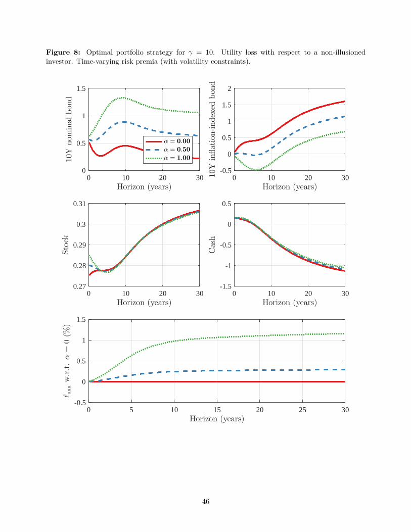
Figure 8: Optimal portfolio strategy for γ = 10. Utility loss with respect to a non-illusionedinvestor. Time-varying risk premia (with volatility constraints).


0

0.5

1

1.5

10Y

nom

inal

bon

d

α = 0.00

α = 0.50

α = 1.00


-0.5

0

0.5

1

1.5

2

10Y

inflation-indexed

bon

d


0.27

0.28

0.29

0.3

0.31

Stock


-1.5

-1

-0.5

0

0.5Cash

0 5 10 15 20 25 30Horizon (years)

-0.5

0

0.5

1

1.5

ℓannw.r.t.α=

0(%

)

46

Figure 9: Optimal portfolio strategy for γ = 10 when the 10-year inflation-indexed or nominalbond is excluded from the investable universe. Utility loss with respect to the case where the fullinvestable universe is available. Time-varying risk premia (with volatility constraints).



0.5

1

1.5

10Y

nom

inal

bon

d

α = 0.00

α = 0.50

α = 1.00


0.2

0.25

0.3

0.35

0.4

Stock


-1

-0.5

0

0.5

Cash


0

0.5

1

1.5

2


(%)



0

0.5

1

1.5

2

10Y

inflation-indexed

bon

d

α = 0.00

α = 0.50

α = 1.00


0.1

0.15

0.2

0.25

0.3

Stock


-1.5

-1

-0.5

0

0.5

Cash


0

0.5

1

1.5

2


(%)

47

Appendix to

Money Illusion:


April 2018

This Appendix is organized as follows. In Section A, we derive the pricing equations for nominal

bonds (A.1) and real bonds (A.2). The derivation of the optimal portfolio strategy is in Section B.

In particular, we derive the optimal portfolio strategy for complete and incomplete markets (B.1),

the optimal portfolio strategy for an infinitely risk-averse individual and constant market prices of

risk (B.2), the utility from suboptimal strategies (B.3) and the certainty equivalent utility loss (B.4).

In Section C, we discuss the empirical findings obtained imposing a zero unexpected inflation risk

premium. Finally, in Section D, we elaborate on the specification with time-varying risk premia

where no volatility constraints are imposed. We discuss the parameter estimates (D.1) and the

portfolio strategy and welfare (D.2).

A Bond pricing

A.1 Nominal bond pricing

We conjecture that the nominal price of a zero-coupon nominal bond has the following functional

form:

B (Xt, τ) = e−yn(Xt,τ)τ = eAN0 (τ)+AN

1 (τ)Xt .

From no-arbitrage arguments, the nominal price B of a nominal bond satisfies the following PDE:

BXΘ(

X − Xt

)

+12

tr(BXXΣ′

XΣX

)+ Bt − RtB = BXΣ′

XΛt

Computing the derivatives:

BX = AN1 B

BXX =(

AN1

)′AN

1 B

A - 1

Bt = −Bτ = −

(∂

∂τAN

0 (τ) +∂

∂τAN

1 (τ) Xt

)

B,

substituting into the PDE the derivatives just computed, as well as the expressions for Rt and Λt:

AN1 Σ′

X (Λ0 + Λ1Xt) = AN1 Θ

(

X − Xt

)

+12

AN1 Σ′

XΣX

(

AN1

)′−

(∂

∂τAN

0 (τ) +∂

∂τAN

1 (τ) Xt

)

−(R0 + R′

1Xt

).

Matching the homogeneous term and the term in Xt:

∂

∂τAN

0 (τ) = AN1

(

ΘX − Σ′XΛ0

)

+12

AN1 Σ′

XΣX

(

AN1

)′− R0, (A.1)

∂

∂τAN

1 (τ) = −AN1

(Θ + Σ′

XΛ1)

− R′1. (A.2)

The nominal rate is given considering the limit for τ → 0:

Rt = R0 + R′1Xt.

The dynamics of the price of a zero-coupon nominal bond expiring at time T is:

dB (Xt, τ)B (Xt, τ)

=[

−

(∂

∂τAN

0 (τ) +∂

∂τAN

1 (τ) Xt

)

+ AN1 Θ

(

X − Xt

)

+12

AN1 Σ′

XΣX

(

AN1

)′]

dt

+AN1 Σ′

Xdzt.

Substituting for the expressions (A.1) and (A.2):


= −

AN

1

(

ΘX − Σ′X

Λ0

)

+ 12AN

1 Σ′X

ΣX

(

AN1

)′− R0

−AN1 (Θ + Σ′

XΛ1) Xt − R′

1Xt

dt

+[

AN1 Θ

(

X − Xt

)

+12

AN1 Σ′

XΣX

(

AN1

)′]

dt

+AN1 Σ′

Xdzt.

We finally obtain:


=[

R0 + R′1Xt + AN

1 Σ′X (Λ0 + Λ1Xt)

]

dt + AN1 Σ′

Xdzt.

A - 2

The instantaneous time-varying risk premium is given by:

AN1 Σ′

X (Λ0 + Λ1Xt) .

A.2 Real bond pricing

We conjecture that the nominal price of a zero-coupon inflation-indexed bond has the following

functional form:

I (Xt, Pt, τ) = Pte−yr(Xt,τ)τ = Pte

AI0(τ)+AI

1(τ)Xt .

From no-arbitrage arguments, the nominal price I of an inflation-indexed bond satisfies the following

PDE:

(IXΣ′

X + IPσ′P Pt

)Λt = IXΘ

(

X − Xt

)

+ IP Ptπt +12

tr(IXXΣ′

XΣX

)+ IXP Σ′

XσP Pt

+12

IP Pσ′PσP P 2

t + It − RtI.

Computing the derivatives:

IX = AI1I,

IP =I

Pt,

IXX =(

AI1

)′AI

1I,

IXP = AI1

I

Pt,

IP P = 0,

It = −Iτ = −

(∂

∂τAI

0 (τ) +∂

∂τAI

1 (τ) Xt

)

I.

Substituting into the PDE the derivatives just computed, as well as the expressions for Rt, πt and

Λt, yields:

(

AI1Σ′

X + σ′P

)

(Λ0 + Λ1Xt) = AI1Θ

(

X − Xt

)

+(π0 + π

′1Xt

)+

12

AI1Σ′

XΣX

(

AI1

)′

+AI1Σ′

XσP −

(∂

∂τAI

0 (τ) +∂

∂τAI

1 (τ) Xt

)

−(R0 + R′

1Xt

).

A - 3

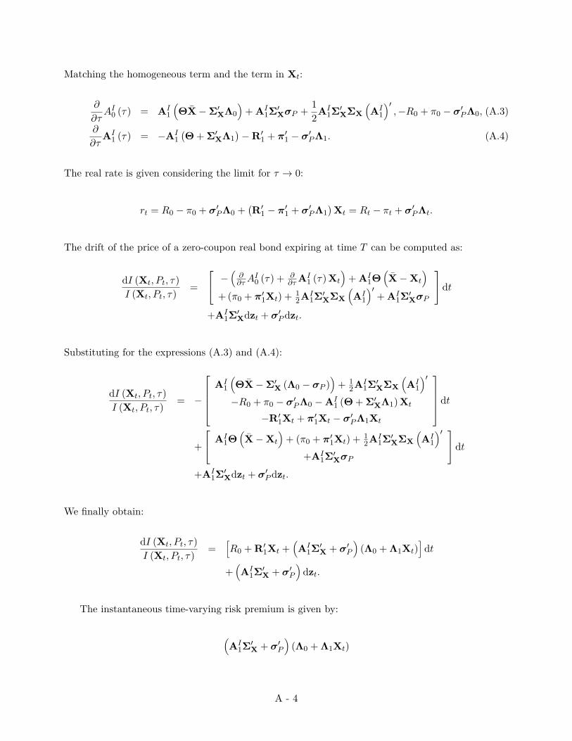
Matching the homogeneous term and the term in Xt:

∂

∂τAI

0 (τ) = AI1

(

ΘX − Σ′XΛ0

)

+ AI1Σ′

XσP +12

AI1Σ′

XΣX

(

AI1

)′, −R0 + π0 − σ

′P Λ0, (A.3)

∂

∂τAI

1 (τ) = −AI1

(Θ + Σ′

XΛ1)

− R′1 + π

′1 − σ

′P Λ1. (A.4)

The real rate is given considering the limit for τ → 0:

rt = R0 − π0 + σ′P Λ0 +

(R′

1 − π′1 + σ

′P Λ1

)Xt = Rt − πt + σ

′P Λt.

The drift of the price of a zero-coupon real bond expiring at time T can be computed as:

dI (Xt, Pt, τ)I (Xt, Pt, τ)

=

−(

∂∂τ

AI0 (τ) + ∂

∂τAI

1 (τ) Xt

)

+ AI1Θ

(

X − Xt

)

+ (π0 + π′1Xt) + 1

2AI1Σ′

XΣX

(

AI1

)′+ AI

1Σ′XσP

dt

+AI1Σ′

Xdzt + σ′P dzt.

Substituting for the expressions (A.3) and (A.4):


= −

AI1

(

ΘX − Σ′X

(Λ0 − σP ))

+ 12AI

1Σ′X

ΣX

(

AI1

)′

−R0 + π0 − σ′P Λ0 − AI

1 (Θ + Σ′X

Λ1) Xt

−R′1Xt + π

′1Xt − σ

′P Λ1Xt

dt

+

AI

1Θ(

X − Xt

)

+ (π0 + π′1Xt) + 1

2AI1Σ′

XΣX

(

AI1

)′

+AI1Σ′

XσP

dt

+AI1Σ′

Xdzt + σ′P dzt.

We finally obtain:


=[

R0 + R′1Xt +

(

AI1Σ′

X + σ′P

)

(Λ0 + Λ1Xt)]

dt

+(

AI1Σ′

X + σ′P

)

dzt.

The instantaneous time-varying risk premium is given by:

(

AI1Σ′

X + σ′P

)

(Λ0 + Λ1Xt)

A - 4

B Portfolio strategy

B.1 Optimal portfolio strategy in incomplete markets

As is well known, the value function can be expressed as:

J (Wt, t) =W

1−γt P

−(1−α)(1−γ)t

1 − γf (Xt, t, T ) (B.5)

With the martingale approach, it can be shown that:

Wt = l− 1

γ Φ− 1

γ

t P−(1−α) 1−γ

γ

t Et

(

ΦT

Φt

(PT

Pt

)(1−α))1− 1

γ

, (B.6)

where Φ0 = 1, P0 = 1 and:

l− 1

γ =W0

E0

[(

ΦT

Φ0

(PT

P0

)(1−α))1− 1

γ

] .

We rewrite wealth as:

Wt = W0Φ− 1

γ

t P−(1−α) 1−γ

γ

t

F (Xt, t, T )F (X0, 0, T )

≡ G (Φt, Pt, Xt, t, T ) , (B.7)

where:

F (Xt, t, T ) = Et

(

ΦT

Φt

(PT

Pt

)(1−α))1− 1

γ

.

Computing the first-order condition of the equation of the value function (B.5) and solving by

Wt, by comparison with (B.6), it immediately follows that f (Xt, t, T ) is such that the value function

can be expressed as follows:

J (Wt, t) =W

1−γt P

−(1−α)(1−γ)t

1 − γ[F (Xt, t, T )]γ , (B.8)

The function F (Xt, t, T ) takes the form:

F (Xt, t, T ) = exp{

12

X′tB3 (τ) Xt + B2 (τ) Xt + B1 (τ)

}

.

A - 5

Remembering that G ≡ Wt, the following no-arbitrage relation holds:

LG + Gt − RtG =(−GΦΦtΛ

′t + GP Ptσ

′P + GXΣ

′X

)Λt, (B.9)

where:

LG = GΦ (−ΦtRt) + GP (Ptπt) + GXΘ(

X − Xt

)

+GΦXΣ′X (−ΦtΛt) + GP XΣ

′X (PtσP ) + GΦP (PtσP )′ (−ΦtΛt)

+12

(

GΦΦ (−ΦtΛt)′ (−ΦtΛt) + GP P (PtσP )′ (PtσP ) + tr

(GXXΣ

′XΣX

))

.

Substituting for the partial derivatives of G:

LG = −1γ

Φ−1t G (−ΦtRt) − (1 − α)

1 − γ

γP −1

t G (Ptπt) +FX

FGΘ

(

X − Xt

)

−1γ

Φ−1t

FX

FGΣ

′X (−ΦtΛt) − (1 − α)

1 − γ

γP −1

t

FX

FGΣ

′X (PtσP )

+ (1 − α)1 − γ

γ2Φ−1

t P −1t G (PtσP )′ (−ΦtΛt)

+12

1γ

(

1 + 1γ

)

Φ−2t G (−ΦtΛt)

′ (−ΦtΛt)

+ (1 − α) 1−γγ

(

1 + (1 − α) 1−γγ

)

P −2t G (PtσP )′ (PtσP )

+tr(

FXX

FGΣ

′XΣX

)

.

Simplifying:

LG

G=

1γ

Rt − (1 − α)1 − γ

γπt +

FX

FΘ(

X − Xt

)

+1γ

FX

FΣ

′XΛt − (1 − α)

1 − γ

γ

FX

FΣ

′XσP − (1 − α)

1 − γ

γ2σ

′P Λt

+12

(1γ

(

1 +1γ

)

Λ′tΛt + (1 − α)

1 − γ

γ

(

1 + (1 − α)1 − γ

γ

)

σ′PσP + tr

(FXX

FΣ

′XΣX

))

.

Substituting into (B.9):

(1γ

Λ′t − (1 − α)

1 − γ

γσ

′P +

FX

FΣ

′X

)

Λt =1γ

Rt − (1 − α)1 − γ

γπt +

FX

FΘ(

X − Xt

)

+1γ

FX

FΣ

′XΛt − (1 − α)

1 − γ

γ

FX

FΣ

′XσP

− (1 − α)1 − γ

γ2σ

′P Λt +

12γ

(

1 +1γ

)

Λ′tΛt

A - 6

+ (1 − α)1 − γ

2γ

(

1 + (1 − α)1 − γ

γ

)

σ′PσP

+12

tr(

FXX

FΣ

′XΣX

)

+Gt

G− Rt.

Rearranging and collecting terms:

0 =(

1γ

− 1)

Rt − (1 − α)1 − γ

γπt +

FX

FΘ(

X − Xt

)

+(

1γ

− 1)

FX

FΣ

′XΛt − (1 − α)

1 − γ

γ

FX

FΣ

′XσP

+(

1 −1γ

)

(1 − α)1 − γ

γσ

′P Λt

+1

2γ

(1γ

− 1)

Λ′tΛt + (1 − α)

1 − γ

2γ

(

1 + (1 − α)1 − γ

γ

)

σ′PσP

+12

tr(

FXX

FΣ

′XΣX

)

+Ft

F.

It is at this point necessary to elaborate on market completeness. The optimal portfolio strategy

is obtained equaling the diffusion terms of the dynamics of (log) wealth, written either as in (B.7)

or as a linear combination of the dynamics of the underlying assets:

Σω =1γ

Λt − (1 − α)1 − γ

γσP + ΣX

(FX)′

F. (B.10)

This n-dimensional equation imposes that the N non-redundant traded assets, for which the volatility

vectors are at the l.h.s., span the dynamics of optimal wealth at the r.h.s.. In the case of complete

markets this happens without issues, as Σ is invertible. If instead markets are incomplete, we follow

Sangvinatsos and Wachter (2005) and impose some further restrictions to make sure that the r.h.s. is

completely spanned by the traded assets. We decompose the r.h.s. of the equation into a contribution

spanned by the traded assets and a contribution orthogonal to the asset space. In order to decompose

the vector of market prices of risk, we write Λt = Λ∗t + ν

∗t , where Λ∗

t belongs to the column space of

the volatility matrix of the traded assets and ν∗t belongs to the null space. We pre-multiply (B.10)

by I − Σ (Σ′Σ)−1

Σ′:

(

I − Σ(Σ

′Σ)−1

Σ′)

Σω

︸︷︷︸

0

=1γ

(

I − Σ(Σ

′Σ)−1

Σ′)

(Λ∗t + ν

∗t )

A - 7

− (1 − α)1 − γ

γ

(

I − Σ(Σ

′Σ)−1

Σ′)

σP

+(

I − Σ(Σ

′Σ)−1

Σ′)

ΣX

(FX)′

F.

This condition will affect the function F , which we still have to determine, and therefore the dynamics

of optimal wealth and the optimal portfolio weights. As(

I − Σ (Σ′Σ)−1

Σ′)

Λ∗t = 0, then:

ν∗t = (1 − α) (1 − γ)

(

I − Σ(Σ

′Σ)−1

Σ′)

σP − γ(

I − Σ(Σ

′Σ)−1

Σ′)

ΣX

(FX)′

F.

Pre-multiplying instead (B.10) by Σ (Σ′Σ)−1

Σ′:

Σ(Σ

′Σ)−1

Σ′Σω

︸︷︷︸

Σω

=1γΣ(Σ

′Σ)−1

Σ′ (Λ∗

t + ν∗t ) − (1 − α)

1 − γ

γΣ(Σ

′Σ)−1

Σ′σP

+Σ(Σ

′Σ)−1

Σ′ΣX

(FX)′

F.

As Σ (Σ′Σ)−1

Σ′ν

∗t = 0, by pre-multiplying again by (Σ′

Σ)−1Σ

′, we obtain the expression for the

optimal portfolio weights (20).

We employ the following notations:

Λ∗t = Σ

(Σ

′Σ)−1

Σ′Λt = Σ

(Σ

′Σ)−1

Σ′ (Λ0 + Λ1Xt) = Λ∗

0 + Λ∗1Xt,

where:

Λ∗0 = Σ

(Σ

′Σ)−1

Σ′Λ0,

Λ∗1 = Σ

(Σ

′Σ)−1

Σ′Λ1,

In the remaining, we also employ the following notations:

σ⊥P =

(

I − Σ(Σ

′Σ)−1

Σ′)

σP ,

Σ⊥X =

(

I − Σ(Σ

′Σ)−1

Σ′)

ΣX.

A - 8

The market prices of risk can therefore be decomposed as:

Λt = Λ∗t + ν

∗t = Λ∗

0 + Λ∗1Xt + (1 − α) (1 − γ)σ⊥

P − γΣ⊥X

(FX)′

F.

We guess the functional form for F (Xt, t, T ):

F (Xt, τ) = exp{

12

X′tB3 (τ) Xt + B2 (τ) Xt + B1 (τ)

}

,

and compute the derivatives:

FX =(

12

X′t

(B3 (τ) + B′

3 (τ))

+ B2 (τ))

F =(

X′tB3 (τ) + B2 (τ)

)

F,

FXX =(

12

X′t

(B3 (τ) + B′

3 (τ))

+ B2 (τ))′ (1

2X′

t

(B3 (τ) + B′

3 (τ))

+ B2 (τ))

F

+12(B3 (τ) + B′

3 (τ))

F

=14(B3 (τ) + B′

3 (τ))′

XtX′t

(B3 (τ) + B′

3 (τ))

F +12

B′2 (τ) X′

t

(B3 (τ) + B′

3 (τ))

F

+12(B3 (τ) + B′

3 (τ))′

XtB2 (τ) F + B′2 (τ) B2 (τ) F +

12(B3 (τ) + B′

3 (τ))

F

= B3 (τ) XtX′tB3 (τ) F + B′

2 (τ) X′tB3 (τ) F + B3 (τ) XtB2 (τ) F

+B′2 (τ) B2 (τ) F + B3 (τ) F,

Ft = −

(12

X′t

ddτ

B3 (τ) Xt +ddτ

B2 (τ) Xt +ddτ

B1 (τ))

F,

where B3 (τ) = B3(τ)+B′3(τ)

2 . The market prices of risk can be rewritten as:

Λt = Λ∗t + ν

∗t

= Λ∗0 + Λ∗

1Xt + (1 − α) (1 − γ)σ⊥P − γΣ⊥

X

(

B3 (τ) Xt + B′2 (τ)

)

= Λ∗0 + (1 − α) (1 − γ)σ⊥

P − γΣ⊥XB′

2 (τ) +(

Λ∗1 − γΣ⊥

XB3 (τ))

Xt

= Λ∗0 + Λ∗

1Xt,

where Λ∗0 = Λ∗

0 + (1 − α) (1 − γ)σ⊥P − γΣ⊥

XB′

2 (τ) and Λ∗1 = Λ∗

1 − γΣ⊥X

B3 (τ). Substituting in the

A - 9

PDE for the expressions of Rt, πt and Λt, as well as for the derivatives of F :

0 =(

1γ

− 1)(R0 + R′

1Xt

)− (1 − α)

1 − γ

γ

(π0 + π

′1Xt

)+(

X′tB3 (τ) + B2 (τ)

)

Θ(

X − Xt

)

+(

1γ

− 1)(

X′tB3 (τ) + B2 (τ)

)

Σ′X

(

Λ∗0 + Λ∗

1Xt

)

− (1 − α)1 − γ

γ

(

X′tB3 (τ) + B2 (τ)

)

Σ′XσP +

(

1 −1γ

)

(1 − α)1 − γ

γσ

′P

(

Λ∗0 + Λ∗

1Xt

)

+1

2γ

(1γ

− 1)(

Λ∗0 + Λ∗

1Xt

)′ (

Λ∗0 + Λ∗

1Xt

)

+ (1 − α)1 − γ

2γ

(

1 + (1 − α)1 − γ

γ

)

σ′PσP

+12

tr((

B3 (τ) XtX′tB3 (τ) + B′

2 (τ) X′tB3 (τ) + B3 (τ) XtB2 (τ) + B′

2 (τ) B2 (τ) + B3 (τ))

Σ′XΣX

)

−

(12

X′t

ddτ

B3 (τ) Xt +ddτ

B2 (τ) Xt +ddτ

B1 (τ))

.

Isolating the term in X′t . . . Xt and solving for d

dτB3 (τ):

ddτ

B3 (τ) = −2B3 (τ) Θ + 2(

1γ

− 1)

B3 (τ)Σ′XΛ∗

1 +1γ

(1γ

− 1)(

Λ∗1

)′Λ∗

1 + B3 (τ)Σ′XΣXB3.

Isolating the term in Xt and solving for ddτ

B2 (τ):

ddτ

B2 (τ) =(

1γ

− 1)

R′1 − (1 − α)

1 − γ

γπ

′1 + X′Θ′B3 (τ) − B2 (τ) Θ

+(

1γ

− 1)(

Λ∗0

)′ΣXB3 (τ) +

(1γ

− 1)

B2 (τ)Σ′XΛ∗

1

− (1 − α)1 − γ

γσ

′PΣXB3 (τ) − (1 − α)

(γ − 1

γ

)2

σ′P Λ∗

1

+1γ

(1γ

− 1)(

Λ∗0

)′Λ∗

1 + B2 (τ)Σ′XΣXB3 (τ) .

Isolating the homogeneous term and solving for ddτ

B1 (τ):

ddτ

B1 (τ) =(

1γ

− 1)

R0 − (1 − α)1 − γ

γπ0 + B2 (τ) ΘX +

(1γ

− 1)

B2 (τ)Σ′XΛ∗

0

− (1 − α)1 − γ

γB2 (τ)Σ′

XσP − (1 − α)(

γ − 1γ

)2

σ′P Λ∗

0

+1

2γ

(1γ

− 1)(

Λ∗0

)′Λ∗

0 + (1 − α)1 − γ

2γ

(

1 + (1 − α)1 − γ

γ

)

σ′PσP

+12

B2 (τ)Σ′XΣXB′

2 (τ) +12

tr(

B3 (τ)Σ′XΣX

)

.

In order to write the optimal portfolio weights, remember that FX

F= X′

tB3 (τ) + B2 (τ). Then,

A - 10

substituting into (20):

ωt =1γ

(Σ

′Σ)−1

Σ′Λt − (1 − α)

1 − γ

γ

(Σ

′Σ)−1

Σ′σP (B.11)

+(Σ

′Σ)−1

Σ′ΣX

(

B3 (τ) Xt + B′2 (τ)

)

.

B.2 Optimal portfolio strategy for an infinitely risk-averse individual and con-

stant market prices of risk

For γ → ∞, in the case of constant market prices of risk (Λ1 = 0), it is possible to write an explicit

solution to the problem. Indeed, in this case B3(τ) → 0 and the optimal portfolio strategy becomes

independent of the current state Xt:

ωt = (1 − α)(Σ

′Σ)−1

Σ′σP +

(Σ

′Σ)−1

Σ′ΣXB′

2 (τ) , (B.12)

where:ddτ

B2 (τ) = −R′1 + (1 − α)π′

1 − B2 (τ) Θ,

for which the solution is:

B2 (τ) =(R′

1 − (1 − α)π′1

) (

e−Θτ − I)

Θ−1.

We can then rewrite the optimal portfolio strategy as:

ωt = (1 − α)(Σ

′Σ)−1

Σ′σP +

(Σ

′Σ)−1

Σ′ΣX

[

R′1

(

e−Θτ − I)

Θ−1]′

(B.13)

− (1 − α)(Σ

′Σ)−1

Σ′ΣX

[

π′1

(

e−Θτ − I)

Θ−1]′

.

Remember that, for constant risk premia, the coefficient AN1 , used for nominal bond pricing,

satisfies the following relation:

∂

∂τAN

1 (τ) = −AN1 (τ) Θ − R′

1, (B.14)

A - 11

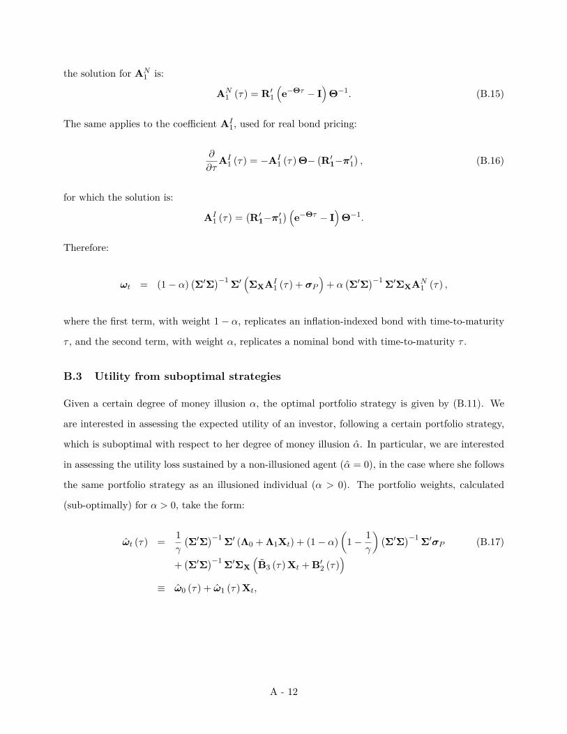
the solution for AN1 is:

AN1 (τ) = R′

1

(

e−Θτ − I)

Θ−1. (B.15)

The same applies to the coefficient AI1, used for real bond pricing:

∂

∂τAI

1 (τ) = −AI1 (τ) Θ−

(R′

1−π′1

), (B.16)

for which the solution is:

AI1 (τ) =

(R′

1−π′1

) (

e−Θτ − I)

Θ−1.

Therefore:

ωt = (1 − α)(Σ

′Σ)−1

Σ′(

ΣXAI1 (τ) + σP

)

+ α(Σ

′Σ)−1

Σ′ΣXAN

1 (τ) ,

where the first term, with weight 1 − α, replicates an inflation-indexed bond with time-to-maturity

τ , and the second term, with weight α, replicates a nominal bond with time-to-maturity τ .

B.3 Utility from suboptimal strategies

Given a certain degree of money illusion α, the optimal portfolio strategy is given by (B.11). We

are interested in assessing the expected utility of an investor, following a certain portfolio strategy,

which is suboptimal with respect to her degree of money illusion α. In particular, we are interested

in assessing the utility loss sustained by a non-illusioned agent (α = 0), in the case where she follows

the same portfolio strategy as an illusioned individual (α > 0). The portfolio weights, calculated

(sub-optimally) for α > 0, take the form:

ωt (τ) =1γ

(Σ

′Σ)−1

Σ′ (Λ0 + Λ1Xt) + (1 − α)

(

1 −1γ

)(Σ

′Σ)−1

Σ′σP (B.17)

+(Σ

′Σ)−1

Σ′ΣX

(

B3 (τ) Xt + B′2 (τ)

)

≡ ω0 (τ) + ω1 (τ) Xt,

A - 12

where τ = T − t and:

ω0 (τ) =1γ

(Σ

′Σ)−1

Σ′Λ0 + (1 − α)

(

1 −1γ

)(Σ

′Σ)−1

Σ′σP +

(Σ

′Σ)−1

Σ′ΣXB′

2 (τ) ,

ω1 (τ) =1γ

(Σ

′Σ)−1

Σ′Λ1 +

(Σ

′Σ)−1

Σ′ΣXB3 (τ) .

The expected utility over terminal wealth (evaluated for α), J (t, Wt, Xt, Pt), is a martingale, as

it represent an expectation of future utility. Thus, it satisfies the following PDE:

∂

∂tJ + LJ = 0,

where LJ is the following differential operator:

LJ = JW Wt

(Rt + ω

′t (τ) Σ′Λt

)+ JXΘ

(

X − Xt

)

+ JP Ptπt

+JXW WtΣ′XΣωt (τ) + JW P WtPtω

′t (τ) Σ′

σP + JXP PtΣ′XσP

+12

JW W W 2t ω

′t (τ) Σ′Σωt (τ) +

12

tr(

JXXΣ′XΣX

)

+12

JP P P 2t σ

′PσP .

We guess the following functional form for J (t, Wt, Xt, Pt):

J (t, Wt, Xt, Pt) =W

1−γt P

−(1−α)(1−γ)t

1 − γH (Xt, t, T ) .

Substituting into the PDE and simplifying:

0 =∂

∂tH + (1 − γ)

(Rt + ω

′t (τ) Σ′Λt

)H + HXΘ

(

X − Xt

)

− (1 − α) (1 − γ) πtH

+ (1 − γ) HXΣ′XΣωt (τ) − (1 − α) (1 − γ)2

ω′t (τ) Σ′

σP H − (1 − α) (1 − γ) HXΣ′XσP

−12

γ (1 − γ) ω′t (τ) Σ′Σωt (τ) H +

12

tr(HXXΣ′

XΣX

)

+12

(1 − α) (1 − γ) (2 − α − γ + αγ)σ′PσP H.

We make a guess on the functional form of H:

H (Xt, τ) = exp{

12

X′tB3 (τ) Xt + B2 (τ) Xt + B1 (τ)

}

.

A - 13

Writing the partial derivatives:

HX =(

12

X′t

(

B3 (τ) + B′3 (τ)

)

+ B2 (τ))

H =(

X′t˜B3 (τ) + B2 (τ)

)

H,

HXX =14

(

B3 (τ) + B′3 (τ)

)′XtX

′t

(

B3 (τ) + B′3 (τ)

)

H +12

B′2 (τ) X′

t

(

B3 (τ) + B′3 (τ)

)

H

+12

(

B3 (τ) + B′3 (τ)

)′XtB2 (τ) H + B′

2 (τ) B2 (τ) H +12

(

B3 (τ) + B′3 (τ)

)

H

=( ˜B3 (τ) XtX

′t˜B3 (τ) + B′

2 (τ) X′t˜B3 (τ) + ˜

B3 (τ) XtB2 (τ) + B′2 (τ) B2 (τ) + ˜

B3 (τ))

H,

∂

∂tH = −

(12

X′t

ddτ

B3 (τ) Xt +ddτ

B2 (τ) Xt +ddτ

B1 (τ))

H,

where ˜B3 (τ) = B3(τ)+B′

3(τ)2 . Substituting into the PDE the partial derivatives, as well as the

quantities Rt, πt, Λt (note that Σ′Λt = Σ′Λ∗t ) and ωt (τ):

0 = −

(12

X′t

ddτ

B3 (τ) Xt +ddτ

B2 (τ) Xt +ddτ

B1 (τ))

(1 − γ)(

R0 + R′1Xt + (ω0 (τ) + ω1 (τ) Xt)

′ Σ′ (Λ0 + Λ1Xt))

+(

X′t˜B3 (τ) + B2 (τ)

)

Θ(

X − Xt

)

− (1 − α) (1 − γ)(π0 + π

′1Xt

)

+ (1 − γ)(

X′t˜B3 (τ) + B2 (τ)

)

Σ′XΣ (ω0 (τ) + ω1 (τ) Xt)

− (1 − α) (1 − γ)2 (ω0 (τ) + ω1 (τ) Xt)′ Σ′

σP

− (1 − α) (1 − γ)(

X′t˜B3 (τ) + B2 (τ)

)

Σ′XσP

−12

γ (1 − γ) (ω0 (τ) + ω1 (τ) Xt)′ Σ′Σ (ω0 (τ) + ω1 (τ) Xt)

+12

tr(( ˜

B3 (τ) XtX′t˜B3 (τ) + B′

2 (τ) X′t˜B3 (τ) + ˜

B3 (τ) XtB2 (τ) + B′2 (τ) B2 (τ) + ˜

B3 (τ))

Σ′XΣX

)

+12

(1 − α) (1 − γ) (2 − α − γ + αγ)σ′PσP .

Isolating the terms in X′t . . . Xt and solving for d

dτB3 (τ):

ddτ

B3 (τ) = 2 (1 − γ) ω′1 (τ) Σ′Λ1 − 2 ˜

B3 (τ) Θ + 2 (1 − γ) ˜B3 (τ) Σ′

XΣω1 (τ)

−γ (1 − γ) ω′1 (τ) Σ′Σω1 (τ) + ˜

B3 (τ) Σ′XΣX

˜B3 (τ) .

A - 14

Isolating the terms in Xt and solving for ddτ

B2 (τ):

ddτ

B2 (τ) = (1 − γ)(R′

1 + ω′0 (τ) Σ′Λ1 + Λ′

0Σω1 (τ))

+X′Θ′ ˜B3 (τ) − B2 (τ) Θ − (1 − α) (1 − γ)π′

1

+ (1 − γ) ω′0 (τ) Σ′ΣX

˜B3 (τ) + (1 − γ) B2 (τ) Σ′

XΣω1 (τ)

− (1 − α) (1 − γ)2σ

′P Σω1 (τ) − (1 − α) (1 − γ)σ′

P ΣX

˜B3 (τ)

−γ (1 − γ) ω′0 (τ) Σ′Σω1 (τ) + B2 (τ) Σ′

XΣX

˜B3 (τ) .

Isolating the homogeneous terms and solving for ddτ

B1 (τ):

ddτ

B1 (τ) = (1 − γ)(R0 + ω

′0 (τ) Σ′Λ0

)+ B2 (τ) ΘX − (1 − α) (1 − γ) π0

+ (1 − γ) B2 (τ) Σ′XΣω0 (τ) − (1 − α) (1 − γ)2

ω′0 (τ) Σ′

σP

− (1 − α) (1 − γ) B2 (τ) Σ′XσP −

12

γ (1 − γ) ω′0 (τ) Σ′Σω0 (τ)

+12

B2 (τ) Σ′XΣXB′

2 (τ) +12

tr( ˜B3 (τ) Σ′

XΣX

)

+12

(1 − α) (1 − γ) (2 − α − γ + αγ)σ′PσP .

B.4 Certainty equivalent utility loss

The certainty equivalent utility loss ℓ, incurred by following a suboptimal strategy, can be measured

in terms of fraction of initial wealth. It can be obtained by solving the following problem:

J (0, W0, X0, P0) = J (0, W0 (1 − ℓ) , X0, P0) .

Developing the r.h.s.:

J (0, W0, X0, P0) =W

1−γ0 (1 − ℓ)1−γ P

−(1−α)(1−γ)0

1 − γ[F (X0, 0, T )]γ = (1 − ℓ)1−γ J (0, W0, X0, P0) ,

and, finally, the initial certainty equivalent loss can be expressed as:

ℓ = 1 −

(

J (0, W0, X0, P0)J (0, W0, X0, P0)

) 11−γ

.

A - 15

It is useful to calculate an annualized certainty equivalent loss, which, for an investment horizon

equal to τ , we evaluate as:

ℓann = 1 −

(

J (0, W0, X0, P0)J (0, W0, X0, P0)

) 1(1−γ)τ

= 1 − (1 − ℓ)1τ .

C Empirical findings imposing a zero unexpected inflation risk pre-

mium

The estimation of the inflation risk premium is an object of debate in the literature concerning

inflation-indexed securities. In our setting, in particular, the unexpected inflation risk premium is

equal to σ′P Λt and determines the difference between the expected inflation πt and the break-even

inflation:

beit = Rt − rt = πt − σ′P Λt. (C.18)

We are interested in assessing whether our empirical findings in terms of portfolio strategy and

welfare are robust with respect to the estimate obtained for the unexpected inflation risk premium.

The base case estimate of this quantity, for the setting with constant risk premia, is non-negligible

and equal to σ′P Λ = 1.17%. We decided to repeat our analysis imposing this quantity to be equal to

zero. In order to do so, we needed to determine a modified vector of constant market prices of risk,

Λ0, so that σ′P Λ0 = 0. Λ is a 5×1 vector. Therefore, we needed to impose four additional constraints

to pin it down. We chose to impose that the risk premia on the 2- and 10-year nominal bonds, as

well as that of the 10-year inflation-indexed bond and the stock, are unchanged with respect to their

base case values. This translates into the following conditions:

AN1 (2) Σ′

X

AB1 (10) Σ′

X

AI1 (10) Σ′

X + σ′P

σ′P

σ′S

Λ0 =

AN1 (2) Σ′

XΛ0

AB1 (10) Σ′

XΛ0(

AI1 (10) Σ′

X + σ′P

)

Λ0

0

σ′SΛ0

.

Figure A.1 shows the optimal portfolio strategy for different degrees of money illusion, as well

as the certainty equivalent annualized loss attributable to money illusion. The results are virtually

A - 16

identical to those obtained for the base case estimate of Λ0 (Figure 6).

[Figure A.1 about here.]

Figure A.2 instead shows the optimal portfolio positions when either the inflation-indexed bond

or the nominal bond are removed from the investable universe, as well as the perceived loss by the

investors with different values of α. The results are, again, very similar to those shown in Figure 7.


Overall, it seems that the conclusions we draw in Section 4 are not sensitive to the estimate of

the realized inflation risk premium.

D Empirical findings with unconstrained volatility of time-varying

risk premia

We report in this section the empirical results obtained where we do not impose any restriction on

the volatility of the risk premia during the estimation phase.

D.1 Estimation

We consider a specification with time-varying risk premia, initially with no restrictions imposed

on the matrix Λ1. As in Christensen et al. (2010), we then iterate the estimation procedure, by

progressively imposing a zero restriction on the element of Λ1 with the lowest t-statistics. We stop

when all the elements of Λ1 have a t-stat higher than 2. The parameter estimates are listed in Table

A.1

[Table A.1 about here.]

The summary statistics and characteristics of the distributions of the most relevant economic

and financial quantities, both historical and as implied by the estimated parameters, are listed in

Table A.2. It is very interesting to note how the model-implied volatility of expected inflation is

affected by considering time-varying risk premia with no restriction on their volatility. In addition,

the estimated risk premia seem to be extremely (and unrealistically) volatile in this case.

A - 17


Table A.3 shows the correlations both from the historical distribution and as implied by the

estimated parameters (for both variable and constant risk premia).


Figure A.3 shows the time series of the model-implied macroeconomic variables, the risk premia

and the maximum achievable Sharpe ratio (considering a 10-year nominal bond, a 10-year inflation-

indexed bond and the stock index). When compared to Figure 2b, it is noticeable how the volatility

of the expected inflation (which is unobservable) is higher in this setting. The annualized bond

risk premia range from −5% to 20%, while the equity premium ranges from −20% to 40%. Their

volatilities also seem to be excessively high. The time series of mean-variance portfolio weights is

even more surprising: for a myopic investor with γ = 10, the portfolio weights of the bonds range

from −600% to 900%. The ex-ante Sharpe ratio (in annual terms) achievable with the mean-variance

portfolio is on average higher than 1, with peaks that reach 5.


D.2 Portfolio strategy and welfare

Portfolio strategy Figure A.4 shows the optimal portfolio strategy when investors have access to

the full investment universe and the state variables are at their long-run means. For short investment

horizons, the optimal strategy is similar to the case where risk premia are constant (Figure 6) or

time-varying with a constrained volatility (Figure 8). When the horizon is increased, the impact of

the time-varying risk premia with unconstrained volatility significantly affects the portfolio strategy.

However, the qualitative results at the long-run mean of the state of the economy are similar to the

other specifications, with an increase of the nominal bond position and a decrease of the real bond

position with α, as well as positions in the stock and cash, which are rather insensitive to α.


A - 18

Utility loss due to money illusion The welfare analysis in the graph at the bottom, showing

the certainty equivalent loss attributable to money illusion, confirms that the welfare effect of money

illusion is substantial. The pattern of the loss is very similar to the case of constant risk premia,

although the size of the relative loss seems to be lower than in the cases of constant or volatility-

constrained risk premia. For example, the annualized loss is about 0.7% for a totally illusioned

investor with a 30-year horizon w.r.t. a rational investor (rather than 1.2% for the case with volatility-

constrained risk premia).

Figure A.4, however, shows relative losses, which somehow hide the actual value of certainty

equivalent returns. In-sample certainty equivalent returns are, in this specification, unrealistically

high. For example, a non-illusioned agent with a 30-year horizon has a certainty equivalent real annu-

alized return equal to 4.36% when risk premia are constant, and equal to 4.50% when risk premia are

time-varying with a constrained volatility. The in-sample certainty equivalent real annualized return

is instead unrealistically equal to 21.27% when risk premia are time-varying with an unconstrained

volatility.

This figure is due to the fact that optimal portfolio positions, as soon as the state of the economy

departs from the long-run mean, quickly assume unrealistically high values. To point out this issue,

we show in Figure A.5 the time series of in-sample portfolio weights, considering a non-illusioned

investor (α = 0) with a 10-year horizon, for the three specifications of risk premia. The weights

are calculated for each date considering the time series of the state variables Xt and the estimated

model parameters. As can be noticed, the positions, which are expressed in fractions of total wealth,

are constant for the case of constant risk premia, time-varying within a realistically implementable

range (from −100% to 200%) for the case of volatility-constrained risk premia, and time-varying

within an unrealistically wide range (from −1500% to 2000%) for the case of unconstrained risk

premia. In particular, the in-sample overfitting of bond risk premia causes incredibly large and

offsetting positions between the nominal bond and the real bond, which correspond to quasi-arbitrage

opportunities. The extremely large in-sample certainty equivalents are a consequence of this same

issue.


A - 19


degrees of money illusion We consider now the case where one of the bonds is removed from the

investable universe. In particular, Figure A.6a shows the case where the inflation-indexed bond is

unavailable. In terms of portfolio positions, qualitatively, the effect of money illusion on the optimal

allocation is similar to the case with volatility-constrained risk premia (Figure 9a), although in this

case the effect of money illusion on the portfolio positions seems to be less pronounced.


We then evaluate the opportunity cost, perceived by investors with different levels of α, of ex-

cluding the real bond. As can be noticed in Figure A.6a, the opportunity cost of excluding the

inflation-indexed bond, although slightly higher for the non-illusioned investor, is huge for any level

of α. In particular, the annualized loss reaches a level of about 8% per annum for a 30-year horizon.

This is a consequence of the fact that, once a bond is excluded from the investable universe, it is

not possible for the investor to exploit the quasi-arbitrage opportunities arising from the in-sample

over-fitted bond risk premia. This result is consistent with empirical results obtained by other stud-

ies relying on unconstrained essentially affine term structure models, such as the huge utility losses

incurred when following suboptimal strategies, as documented by Sangvinatsos and Wachter (2005)

and Barillas (2011), or the extremely high sensitivity to parameter uncertainty, as documented by

Feldhütter et al. (2012).

Finally, Figure 9 shows the complementary case, where the nominal bond is excluded from the

investable universe. As expected, the annualized loss is slightly higher for the money-illusioned

investor, but the value of about 7.5% per annum, applicable to all investors, seems to be unrealistically

high.

A - 20

Table A.1: Parameter estimates when no constraints on the volatility of risk premia are imposed.

The table shows the maximum-likelihood estimates of the model parameters. The values in parenthe-ses are the standard errors of the estimates. Starting from an unrestricted matrix Λ1, the estimation isiterated by progressively imposing a zero restriction on the element of Λ1 with the lowest t-statistics.The results reported in the table correspond to the estimate obtained when all the elements of Λ1

have a t-stat higher than 2. The sample period runs from January 1999 until January 2016.

R0 R1 π0 π1 Θ σBǫ σI

ǫ

0.0185 0.3627 0.0206 0.0692 0.0647 0.7241 1.0434 0.0012 0.0007(0.0001) (0.0013) (0.0021) (0.0050) (0.0032) (0.3668) (0.0371) (0.0000) (0.0000)

−0.4186 −0.6482 0.0216 0.6808 −0.3107(0.0053) (0.0957) (0.0019) (0.1412) (0.0210)0.3255 −1.9020 −0.0224 0.1209 2.2387

(0.0135) (0.4692) (0.0018) (0.1825) (0.4280)Λ0 Λ1 ΣX σP σS

−0.6897 0 −62.1901 0 0.0205 0.0069 −0.0050 −0.0001 0.0420(0.0338) (17.7928) (0.0010) (0.0009) (0.0007) (0.0007) (0.0105)0.4655 0 0 0 0 0.0123 0.0021 −0.0008 −0.0358

(0.0518) (0.0006) (0.0007) (0.0007) (0.0108)−0.2056 0 −38.2214 −224.6685 0 0 0.0088 −0.0043 −0.0426(0.0613) (18.3875) (46.5592) (0.0004) (0.0006) (0.0101)1.2118 0 0 −210.3079 0 0 0 0.0087 −0.0155

(0.2718) (50.0411) (0.0004) (0.0095)0.7563 −9.0400 0 0 0 0 0 0 0.1399

(0.2746) (4.5026) (0.0069)

A - 21

Table A.2: Historical and model-implied summary statistics when no constraints on the volatilityof risk premia are imposed.

The table shows annualized historical and model-implied means and volatilities of bond yields, equitylog returns, realized inflation and their model-implied means and volatilities. The table also showsthe model-implied means and volatilities of the bond risk premia, the equity risk premium, thenominal risk-free rate and the expected inflation.

Time seriesMean value Volatility

Estimation Data Estimation Data




3M nominal risk premium 0.12% 0.16%6M nominal risk premium 0.25% 0.29%1Y nominal risk premium 0.52% 0.49%2Y nominal risk premium 1.07% 1.18%3Y nominal risk premium 1.62% 2.33%5Y nominal risk premium 2.55% 5.07%7Y nominal risk premium 3.21% 7.42%10Y nominal risk premium 3.73% 9.52%

5Y real risk premium 2.19% 5.44%7Y real risk premium 2.70% 6.12%10Y real risk premium 3.25% 7.10%

Realized inflation risk premium 1.11% 0.93%Equity risk premium 5.02% 14.95%Nominal risk-free rate 1.85% 0.61%


A - 22

Table A.3: Correlations between asset returns and economic variables when no constraints on thevolatility of risk premia are imposed.

Panel (a) shows unconditional correlations between nominal and real bond returns, stock returnsand realized inflation, calculated from the monthly time series. Panel (b) reports one-month condi-tional pairwise correlations between nominal and real bond returns, stock returns, realized inflation,nominal interest rate, expected inflation and real interest rate.

(a) Data

3M nom 1Y nom 2Y nom 5Y nom 10Y nom 5Y real 10Y real Equity CPI

3M nom 1.0001Y nom 0.658 1.0002Y nom 0.471 0.924 1.0005Y nom 0.257 0.708 0.889 1.00010Y nom 0.108 0.499 0.669 0.904 1.0005Y real −0.000 0.311 0.409 0.501 0.476 1.00010Y real −0.009 0.322 0.440 0.623 0.682 0.910 1.000Equity −0.160 −0.299 −0.352 −0.323 −0.253 0.038 0.000 1.000

CPI −0.124 −0.150 −0.139 −0.190 −0.234 0.350 0.156 0.070 1.000

(b) Time-varying risk premia without volatility restrictions


3M nom 1.0001Y nom 0.929 1.0002Y nom 0.754 0.942 1.0005Y nom 0.412 0.712 0.905 1.00010Y nom 0.212 0.538 0.780 0.968 1.0005Y real 0.087 0.214 0.327 0.483 0.616 1.00010Y real 0.057 0.273 0.458 0.670 0.798 0.962 1.000Equity −0.233 −0.313 −0.344 −0.306 −0.235 0.090 0.004 1.000

CPI 0.057 −0.049 −0.132 −0.179 −0.140 0.286 0.161 0.067 1.000R −0.974 −0.852 −0.631 −0.255 −0.060 −0.070 0.009 0.173 −0.128 1.000π −0.327 −0.500 −0.580 −0.521 −0.359 0.494 0.272 0.390 0.459 0.188 1.000r 0.036 0.131 0.181 0.136 −0.004 −0.788 −0.597 −0.293 −0.477 0.063 −0.904 1.000

A - 23

Figure A.1: Optimal portfolio strategy for γ = 10. Utility loss with respect to a non-illusionedinvestor. Constant risk premia and zero realized inflation risk premium.


0

0.5

1

1.5

2

10Y

nom

inal

bon

d

α = 0.00

α = 0.50

α = 1.00


-0.5

0

0.5

1

1.5

10Y

inflation-indexed

bon

d


0.27

0.28

0.29

0.3

Stock


-1.5

-1

-0.5

0

0.5Cash

0 5 10 15 20 25 30Horizon (years)

-0.5

0

0.5

1

1.5

ℓannw.r.t.α=

0(%

)

A - 24

Figure A.2: Optimal portfolio strategy for γ = 10 when the 10-year inflation-indexed or nominalbond is excluded from the investable universe. Utility loss with respect to the case where the fullinvestable universe is available. Constant risk premia and zero realized inflation risk premium.



0.5

1

1.5

2

10Y

nom

inal

bon

d

α = 0.00

α = 0.50

α = 1.00


0.25

0.3

0.35

0.4

0.45

Stock


-1.5

-1

-0.5

0

0.5

Cash


0

0.5

1

1.5


(%)



0

0.5

1

1.5

2

10Y

inflation-indexed

bon

d

α = 0.00

α = 0.50

α = 1.00


0.05

0.1

0.15

0.2

0.25

Stock


-1.5

-1

-0.5

0

0.5

Cash


0

1

2

3


(%)

A - 25

Figure A.3: Time series of macroeconomic variables, risk premia, mean-variance portfolio positionsand the maximum achievable Sharpe ratio (considering a 10-year nominal bond, a 10-year inflation-indexed bond, the stock index and γ = 10). Time-varying risk premia (unconstrained volatility).

2000 2002 2005 2007 2010 2012 2015

-0.05

0

0.05

0.1



2000 2002 2005 2007 2010 2012 2015-0.2

0

0.2

0.4

0.6Risk premia


2000 2002 2005 2007 2010 2012 2015

-5

0

5

10Weights mean-variance portfolio (γ = 10)


2000 2002 2005 2007 2010 2012 20150

1

2

3

4

5


A - 26

Figure A.4: Optimal portfolio strategy for γ = 10. Utility loss with respect to a non-illusionedinvestor. Time-varying risk premia (unconstrained volatility).


-0.5

0

0.5

1

10Y

nom

inal

bon

d

α = 0.00

α = 0.50

α = 1.00


-1

0

1

2

3

10Y

inflation-indexed

bon

d


0.28

0.3

0.32

0.34

0.36

0.38

Stock


-2

-1.5

-1

-0.5

0

0.5Cash

0 5 10 15 20 25 30Horizon (years)

-0.2

0

0.2

0.4

0.6

0.8

ℓannw.r.t.α=

0(%

)

A - 27

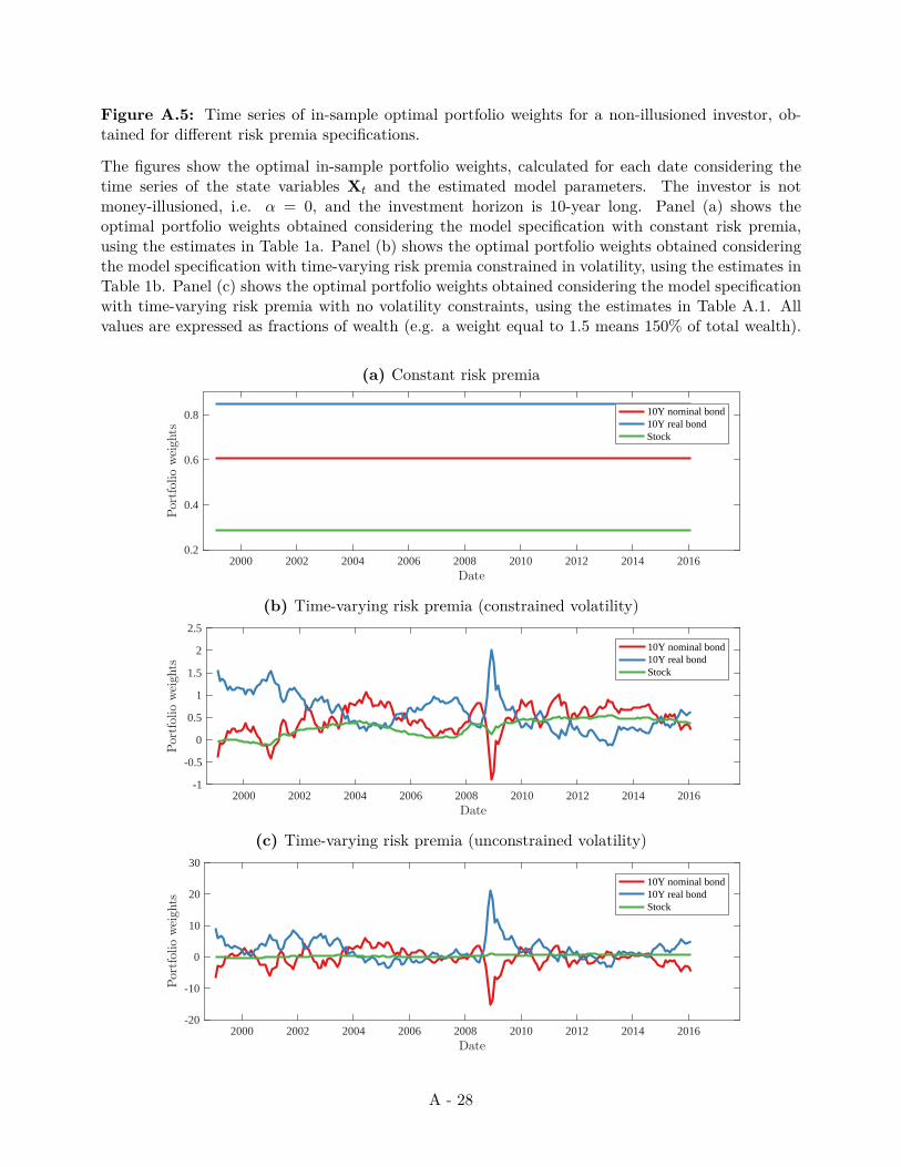
Figure A.5: Time series of in-sample optimal portfolio weights for a non-illusioned investor, ob-tained for different risk premia specifications.

The figures show the optimal in-sample portfolio weights, calculated for each date considering thetime series of the state variables Xt and the estimated model parameters. The investor is notmoney-illusioned, i.e. α = 0, and the investment horizon is 10-year long. Panel (a) shows theoptimal portfolio weights obtained considering the model specification with constant risk premia,using the estimates in Table 1a. Panel (b) shows the optimal portfolio weights obtained consideringthe model specification with time-varying risk premia constrained in volatility, using the estimates inTable 1b. Panel (c) shows the optimal portfolio weights obtained considering the model specificationwith time-varying risk premia with no volatility constraints, using the estimates in Table A.1. Allvalues are expressed as fractions of wealth (e.g. a weight equal to 1.5 means 150% of total wealth).


2000 2002 2004 2006 2008 2010 2012 2014 2016Date

0.2

0.4

0.6

0.8

Portfolio

weigh

ts

10Y nominal bond10Y real bondStock

(b) Time-varying risk premia (constrained volatility)

2000 2002 2004 2006 2008 2010 2012 2014 2016Date

-1

-0.5

0

0.5

1

1.5

2

2.5

Portfolio

weigh

ts


(c) Time-varying risk premia (unconstrained volatility)

2000 2002 2004 2006 2008 2010 2012 2014 2016Date

-20

-10

0

10

20

30

Portfolio

weigh

ts


A - 28

Figure A.6: Optimal portfolio strategy for γ = 10 when the 10-year inflation-indexed or nominalbond is excluded from the investable universe. Utility loss with respect to the case where the fullinvestable universe is available. Time-varying risk premia (unconstrained volatility).



0.5

1

1.5

2

10Y

nom

inal

bon

d

α = 0.00

α = 0.50

α = 1.00


0.2

0.3

0.4

0.5

Stock


-1.5

-1

-0.5

0

0.5

Cash


0

5

10


(%)



0

1

2

3

10Y

inflation-indexed

bon

d

α = 0.00

α = 0.50

α = 1.00


0.2

0.3

0.4

0.5

Stock


-2

-1

0

1

Cash


0

2

4

6

8


(%)

A - 29

money illusion: a rationale for the tips puzzle - … annual meetings/2018-milan...money illusion: a...

Documents