Monitoring Forests Through Succesive InventoriesModerator: James T. Bones

Charles T. Scott, An Overview of Fixed Versus Variable-Radius Plots for SuccessiveInventories

Michael Koehl, Designing a New National Forest Inventory for Switzerland

John R. Mills, Developing ATLAS Growth Parameters From Forest Inventory Plots

Richard Birdsey and Hans Schreuder, Forest Change - An Assessment of NationwideForest Inventory Methods

Charles T. Scott and James Alegria, Fixed-Versus Variable-Radius Plots for ChangeEstimation

William H. McWilliams, Assessing Pine Regeneration for the South Central United States

James M. Hill, Joshua L. Royte, Jil M. Swearingen, Keith Van Ness, William Warncke,and John E. Hench, A Permanent Plot System Designed for Making Natural ResourcesManagement Decisions in a Rapidly Urbanizing County

Piermaria Corona and Agostino Ferrara, INFOR_1: An Analysis Program for PermanentForest Inventories With Systematic Sampling

Susan L. Stout, Inventory to Support Silvicultural Decisions

M.R. Carroll, Funding, Pests and Hardwood Log Grades: User-Driven Cooperative Projectsin the North Central States

An Overview of Fixed Versus Variable-Radius Plotsfor Successive Inventories

Charles T. ScottResearch Forester

USDA Forest ServiceNortheastern Forest Experiment Station

5 Radnor Corp. Center, #200Radnor, PA 19087

ABSTRACT

Since Bitterlich introduced point or variable-radius sampling in 1947, many investigators havecompared it with fixed-area sampling for estimation of current attributes. A partial review of theliterature that compares the two methods is given for successive or continuous forest inventories. Thesampling methods are described in the areas of field implementation, components of change estimation,comparison methods used, and efficiency for both current and change estimates. Point sampling is goodfor current attributes which are related to tree size, but this advantage diminishes for changeestimation.

INTRODUCTION

Forest inventories are usually based on one of two sampling systems, fixed-area orvariable-radius sampling. Fixed-area samples are often circular (fixed-radius) and have been used fordecades, particularly with Continuous Forest Inventories (Ware and Cunia 1962). Variable-radius orpoint sampling was introduced by Bitterlich (1947). Point sampling is very efficient for estimating basalarea per acre. Measuring tree diameter was not required—only a tree count using a prism or anglegauge (Grosenbaugh 1952). Investigators have used many different methods to compare point samplingagainst the time-honored fixed-area sampling rule to ensure that the estimates were both accurate andcost-effective.

Initially, point sampling was used only for quick, temporary surveys without monumenting eachplot. Over time the need for estimates of change between successive surveys became important. Insome cases, the only plots available for remeasurement were point samples. Many articles haveappeared in the literature on how to estimate growth from point samples. Eventually, a fewinvestigators compared fixed- and variable-radius sampling for change estimation. This article presentsan overview of this history, but focuses on comparing fixed plots and point samples for successivesurveys. No attempt has been made to give a complete bibliography of the subject.

PRACTICAL ASPECTS

Much of the initial appeal of point sampling was that sample trees need not be visited to computeprecise estimates of basal area and volume (Grosenbaugh and Stover 1957). For successive surveys,components of change (ingrowth, accretion, mortality, and removals) can only be estimated bymonumenting the plot and identifying the location of each tree (Beers 1962). Thus, a primary benefit ofpoint sampling is lost for successive surveys.

How to handle borderline trees with point sampling has long been a concern. Zeide and Troxell(1979) and Wiant et al. (1984) investigated concerns over missing trees as the distance between thesample point and tree increases. Grosenbaugh (1952) and Solomon (1975) also found underestimates

97

using a small basal area factor (BAF). Brush and trees obscure the observer's vision. Point samples aremore affected than fixed plots, so Wiant et al. and Zeide and Troxell recommended using large BAF'sto minimize the number of missed trees.

Another disturbing factor is that the effective plot area for a tree changes as it grows, thuschanging the number of trees per acre the tree represents (Beers and Miller 1964).

COMPONENTS OF CHANGE ESTIMATION

The components of change usually include ingrowth, accretion (survivor growth), mortality,removals (cut), and net change. These components can be applied to a variety of attributes, such asnumber of stems, basal area, or volume per acre. The methods for estimating these are simple for fixedplots. When Beers (1962) introduced methods for estimating components of change from point samples,he noted some "complications." The primary problems were: 1) not all new trees are ingrowth, somecan be "nongrowth" trees, 2) the number of trees (expansion factor) changes over time for survivortrees, and 3) the components of change did not necessarily sum to the difference between the twosurvey estimates (see Roesch et al. 1989).

"Nongrowth" trees were above the merchantability limit at the previous survey and were notsampled with the prism, but are large enough now to be sampled with the prism. Various authors havetried different methods of handling these new trees and have called them either "ongrowth" or"nongrowth" trees (Beers 1962, Beers and Miller 1964, Nishizawa 1967, and Martin 1982). VanDeusen et al. (1986) used diameter growth models to distinguish between nongrowth and true ingrowthtrees and included their current volume as survivor growth. Roesch et al. (1989) included thenongrowth component in a more natural way by including only their estimated growth.

The second problem is one of choosing an expansion factor to apply to survivor trees. Onesuggestion was to use only the previous expansion factor (Myers and Beers 1968). Van Deusen et al.(1986) suggested using the current expansion factor for the current attribute and the previous one forthe previous attribute, then taking the difference. This can lead to negative growth estimates forsurvivor trees, but is offset by including all of the current volume of nongrowth trees—not just thegrowth. Other approaches have been tried by Martin (1982) and lies and Beers (1983). Roesch et al.(1989) used only the current expansion factor for both previous and current attributes for both survivorand nongrowth trees. However, the additivity criterion was not satisfied without improving the estimateat Time 1 based on information recorded at Time 2.

METHODS OF COMPARING SAMPLE DESIGNS

The two primary methods of comparing the sampling designs are to compute the relativeprecision (ignoring costs) or the relative efficiency. Many studies have reported the relative precisionof particular plot designs that were tried in the field (Grosenbaugh and Stover 1957, Solomon 1975).The primary benefit of these studies was to verify that point samples gave accurate results. Theyprovided little indication of which sampling rule was most cost-effective.

Relative efficiency can be computed in one of two ways: taking the ratio of variances for a fixedcost, or taking the ratio of costs for fixed precision. When computing relative efficiency, a costfunction is implied. Many investigators have simply observed costs for specific plot designs and madedirect comparisons (Avery and Newton 1965, Barrett and Carter 1968). Stage (1958) presented a graphrelating fixed plot size and BAF for individual tree diameters. Banyard (1976) fixed the cost bychoosing fixed plot and point sample sizes so that the number of trees were equal. Several investigatorsused detailed cost functions to closely approximate field conditions (Nyyssonen and Kilkki 1965,Nichols 1980, Scott 1981a, Scott et al. 1983). When these cost functions were associated with a model

98

for plot variability (precision), optimal plot designs could be found. Either the cost was minimized fora specified precision level or variance was minimized for fixed cost.

Cost Functions

Investigators have used a variety of cost functions. Functions for single plots usually involveoverhead costs and the cost per plot times the number of plots. Other studies included the cost of travelbetween sample plots as a function of the density of plots in the population (lessen 1942, Humphreys1979). In the case of cluster sampling, Hansen et al. (1953) present a simple cost function. In forestry,Anagnostopoulos (1966), Nyyssonen et al. (1971), O'Regan et al. (1973), Nichols (1980), and Scott(1981a) presented detailed cost functions for cluster sampling. The approach of Scott (1981a) was tomodel actual survey costs and the variation between clusters as functions of the cluster designvariables. The cluster design variables were the number of plots per cluster (m), the average distancebetween plots (d), and the size of each plot (z).

Precision Models

Perhaps the first model to relate variability to plot design characteristics was introduced by Smith(1938). This model form has been used frequently in forestry applications (Freese 1961, Ziede 1980,Wiant and Yandle 1980). Nyyssonen et al. (1971) and Scott (1981a) expanded Smith's model form toother cluster design variables.

Optimization

Many investigators have used optimization techniques to identify cost-effective sampling designs.Perhaps the most direct method is to use theoretical methods. O'Regan and Arvanitis (1966) computedthe relative efficiency of fixed plots and point samples after analytically minimizing cost subject toconstraints on precision models. Sukwong et al. (1971), Matera (1972), Oderwald (1975, 1979, 1981),Ranneby (1980), and Martin (1983) used similar mathematical techniques but assumed cost wasconstant. However, they introduced characteristics of the population, such as spatial distribution, intothe precision model in an attempt to generalize the results. Gambill et al. (1985) did not compare thetwo sampling methods, but presented tables of the optimal fixed plot and point sample sizes for varyingtract sizes, coefficients of variation, and measurement times.

When the cost or precision models become too complicated to derive mathematical optima,numerical optimization techniques such as linear programming have been used (Hazard and Promnitz1974, Hazard 1976, Marshall and Nautiyal 1980, Morris 1981). Others have used Monte Carlosimulation techniques. A real or simulated stem map of a forest can be used to test many samplingdesigns without performing additional field work (Kulow 1966; Arvanitis and O'Regan 1967, 1972;Kaltenberg 1978).

COMPARISONS FOR CURRENT ESTIMATES

Soon after Grosenbaugh (1952) introduced point sampling to the United States forestry literature,many investigators began comparing it with fixed plot sampling for estimating current values. Usingtheoretical methods, Sukwong et al. (1971) and Matern (1972) state that fixed plot sampling mustalways sample more trees than point samples to yield the same precision. They provide general .solutions for comparing fixed plots and point samples when costs are ignored by including the effectsof clustering and diameter distributions. Oderwald (1981) states that point samples perform best whenthere is a wide range of diameters.

99

John (1964) found that point samples are better for estimation of cover type. Lindsey (1956)found point samples insufficient for density estimation, so recommended augmenting them withquadrats. Lindsey et al. (1958) found point samples to be more efficient than fixed plots whenestimating both density and basal area. Nyyssonen and Kilkki (1965) compared several fixed plot andpoint sample sizes with the 10-point prism cluster often used by the USDA Forest Service (Scott1981b). Fixed-plot sizes of 0.1—0.125 ha were the most efficient of the designs considered for volumeestimation over a range of conditions. O'Regan and Arvanitis (1966) state that fixed plots were mostefficient for estimating number of trees and point samples are most efficient for estimating basal area.No conclusion was given in the case where both attributes are of interest.

Joshi and Tomar (1976) found point samples to be more cost-effective even though pointsampling required more 1 m2/ha BAF plots than 0.05—0.125 ha fixed plots. Banyard (1976) foundpoint samples to be 2.78 times more efficient than fixed plots for current basal area estimates intropical rain forests. He also noted that the stand table for all but the smallest diameter class was betterestimated with point samples due to the higher rate of sampling of large trees. Kulow (1966)recommended a 10 BAF plot over fixed plots for basal-area estimation. Barrett and Carter (1968) found20-BAF plots to be 67—98 percent more efficient than 1/10-acre plots for volume estimation. Averyand Newton (1965) found 1/10-acre and 10-BAF plots to perform equally well for bottomlandhardwoods in Georgia, but 1/10- or 1/20-acre plots were more efficient for natural pine stands.

For northern Ontario, Payandeh (1974) found that 1) most coniferous forests are highlyclustered, 2) most hardwood forests are randomly distributed, and 3) uniformly distributed naturalstands are rare. Martin (1983) states that if the attribute of interest is independent of, or negativelycorrelated with, basal area, then fixed plots are always more precise (see also Oderwald 1975, 1979,1981). He provides formulas for a critical coefficient of correlation under random or clustered spatialdistributions. Correlations with basal area greater than the critical value indicate that point samples aremore precise. Oderwald (1981) states that "point sampling is more precise than plot sampling for thesame effort in the clumped and random spatial patterns, but plot sampling is more precise in the squarelattice pattern." Applying Payandeh's results, we would expect that point sampling is more precise fornatural stands, and plot sampling is more precise for planted stands. However, the study by Avery andNewton (1965) does not support this.

COMPARISONS FOR CHANGE ESTIMATES

The work of Martin (1983) focused on the relative precision of growth estimators, but his resultsapply equally well to the estimation of current values discussed in the proceeding section. Thus therelative precision of fixed plots to point samples depends on the spatial distribution and the correlationof the attribute of interest to basal area.

Arvanitis and O'Regan (1967) used simulation techniques to compare fixed plots and pointsamples for the estimation of current number of trees, number of ingrowth trees, current basal area,and gross basal-area growth (ingrowth plus accretion). If we assume that measurement costs were thesame for trees sampled on fixed plots versus point samples, fixed plots were more efficient for allattributes except current basal area. Arvanitis and O'Regan (1967, p. 149) found gross basal-areagrowth to be "more highly correlated with number of trees than with basal area itself when estimatesare based on point sampling." Elsewhere in these proceedings, Scott and Alegria found that basal areaof ingrowth trees was more efficiently estimated on fixed plots, but basal-area accretion was moreefficiently estimated on point samples. Thus the results of Arvanitis and O'Regan may be due in part tousing gross basal-area growth rather the basal-area accretion.

Ranneby (1980) extended Matern's (1972) work to the estimation of basal-area growth. He statesthat the advantage of point samples is less when estimating basal-area growth versus current basal area.

100

The decrease is substantial if no cutting has occurred. He states that the efficiency of point samples forestimating current basal area can also hold for estimating removals. The empirical results of Scott andAlegria agree in part with Ranneby's statements. Scott and Alegria found removals to be efficientlyestimated using point samples, but the relative efficiency of basal-area growth was as least as large asfor current basal area.

CONCLUSIONS AND SUMMARY

The practical problems with using point sampling for permanent plots in successive inventorieslargely have been overcome through the use of appropriate and efficient growth estimators. Manycomparisons of fixed- and variable-radius sampling have been performed while ignoring costs. Manyothers have addressed only current basal area estimation. More work needs to done using mathematicaland numerical optimization techniques to find cost-effective designs for a variety of current and changeattributes across a range of diameter and spatial distributions.

In general, fixed plots were found to be more efficient for estimation of the current number ofstems. Point samples were more efficient for current basal area and volume. The efficiency advantageof point samples is reduced when estimating accretion in basal area and volume. Fixed plots are likelyto be more efficient for estimation of the change in number of stems and of ingrowth basal area andvolume. As with estimation of current values, the choice between fixed plots and point samples forestimating change depends on the relative importance of estimating number of trees versus basal areaor volume.

LITERATURE CITED

Anagnostopoulos, C.J., 1966: The most efficient number of elements and distance between themin a cluster sampling unit. M.S. thesis, State University of New York, Syracuse, 72 pp.

Arvanitis, L.G., O'Regan, W.G., 1967: Computer simulation and economic efficiency in forestsampling. Hilgardia, vol. 38, pp. 133—164.

Arvanitis, L.G., O'Regan, W.G., 1972: Cluster or satellite sampling in forestry: a Monte Carlocomputer simulation study. Proceedings Third Conference IUFRO Advisory Group of ForestStatisticians, Jouy-en-Josas, France, pp. 191—205.

Avery, Gene and Newton, R., 1965. Plot sizes for timber cruising in Georgia. Journal ofForestry, vol. 63, no. 12, pp. 930-932.

Banyard, S.G., 1976: A comparison between point sampling and plot sampling in tropical rainforest based on a concept of the equivalent relascope plot size. Commonwealth Forestry Review, vol.54, pp. 312-320.

Barrett, J.P. and Carter, J.F., 1968: Comparing methods of sampling a white pine stand. Journalof Forestry, vol. 66, no. 11, pp. 861-863.

Beers, T.W., 1962: Components of forest growth. Journal of Forestry, vol. 60, no. 4, pp.245-248.

Beers, T.W. and Miller, C.I., 1964. Point sampling: research results, theory, and applications.Purdue University Research Bulletin 786. 56 pp.

101

Bitterlich, W., 1947: Die winkezahlmessung. Allg. Forst-u. Hozwirtsch. Ztg., vol. 58, pp.94-96.

Freese, F., 1961: Relation of plot size to variability: an approximation. Journal of Forestry, vol.59, p. 679.

Gambill, C.W., Wiant, H.V., Jr. and Yandle, D.O., 1985: Optimum plot size and BAF. ForestScience vol, 31, no. 3, pp. 587-594.

Grosenbaugh, L.R., 1952: Plotless timber estimates—new, fast, easy. Journal of Forestry, vol.50, no. 1, pp. 32-37.

Grosenbaugh, L.R. and Stover, W.F., 1957: Point sampling compared with plot sampling insoutheast Texas. Forest Science, vol. 3, no. 1, pp. 2—14.

Hansen, M.H., Hurwitz, W.N., and Madow, W.G., 1953: Sample Survey Methods and Theory,Vol. I., John Wiley and Sons, NY, 638 pp.

Hazard, J.W., 1976: Optimization in multi-resource inventories. Proceedings Inventory Designand Analysis. W.E. Prayer, G.B. Hartman, and D.R. Bower, editors. Society of American Forestersworkshop, pp. 170-180.

Hazard, J.W. and Promnitz, L.C., 1974. Design of successive forest inventories: optimization byconvex mathematical programming. Forest Science, vol. 20, pp. 117—127.

Humphreys, C.P., 1979: The cost of sample survey designs. Proceedings American StatisticalAssociation, Survey Research Methods Section, pp. 395—400.

lies, K. and Beers, T.W., 1983: Growth information from variable plot sampling. ProceedingsRenewable Resource Inventories for Monitoring Changes and Trends, College of Forestry, OregonState University, Corvallis, Society of American Foresters 83-14. pp. 693—694.

Jessen, R.J., 1942: Statistical investigation of a sample survey for obtaining farm facts. IowaAgricultural Experiment Station Research Bulletin 304, 104 pp.

John, H.H., 1964: Comparative precision levels in forest inventory estimating using samplingwith probability proportional to frequency and sampling with probability proportional to size. Ph.D.dissertation, University of Minnesota, St. Paul. 76 pp.

Joshi, S.C. and Tomar, M.S., 1976: Investigations on plot size vis-a-vis point sampling: a pilotstudy. Indian Forester, vol. 102, no. 10, pp. 701-711.

Kaltenberg, M.C., 1978: Evaluation of regeneration sampling methods: a Monte Carlo analysisusing simulated stands. State of Washington, Department of Natural Resources, Report 39, 50 pp.

Kulow, D.L., 1966: Comparison of forest sampling designs. Journal of Forestry, vol. 64, no. 7,pp. 469-474.

Lindsey, A.A., 1956: Sampling methods and community attributes in forest ecology. ForestScience, vol. 2, no. 1, pp. 287-296.

Lindsey, A.A., Barton, J.D., Jr., and Miles, S.R., 1958: Field efficiencies of forest samplingmethods. Ecology, vol. 39, no. 3, pp. 428—444.

102

Marshall, P.L. and Nautiyal, J.C., 1980: Optimal sampling size in multivariate forestinventories: a programming procedure. Canadian Journal of Forest Research, vol. 10, no. 4, pp.579-585.

Martin, G.L., 1982: A method for estimating ingrowth on permanent horizontal sample points.Forest Science, vol. 28, no. 1, pp. 110—114.

Martin, G.L., 1983: The relative efficiency of some forest growth estimators. Biometrics, vol.39, no. 3, pp. 639-650.

Matern, B., 1972: The precision of basal area estimates. Forest Science, vol. 18, no. 2, pp.123-125.

Morris, M.J., 1981: Plot configurations for multiresource purposes in the West. ProceedingsIn-Place Resource Inventories: Principles and Practices. Orono, ME, Society of American Foresters82-2, pp. 375-378.

Myers, C.C. and Beers, T.W., 1968: Point sampling for forest growth estimation. Journal ofForestry, vol. 66, no. 12, pp. 927-929.

Nichols, J.D., 1980: Intra-cluster correlation in sample design. Proceedings Arid Land ResourceInventories: Developing cost-efficient methods. USDA Forest Service General Technical ReportWO-28, pp. 142-147.

Nishizawa, M., 1967: Growth estimation by the angle method. Proceedings 14th CongressInternation Union of Forest Research Organizations, Munich, Part VI, Section 25, pp. 410—425.

Nyyssonen, A. and Kilkki, P., 1965: Sampling a stand in forest survey. Acta Forestalia Fennica,vol. 79, no. 4, 20 pp.

Nyyssonen, A., Roiko-Jokela, P., and Kilkki, P., 1971: Studies on improvement of theefficiency of systematic sampling in forest inventory. Acta Forestalia Fennica, vol. 116, 26 pp.

Oderwald, R.G., 1975: The effect of spatial distribution on the efficiency of a class ofprobability proportional to size sampling estimators. Unpubl. Ph.D. dissertation, University of Georgia,Athens. 63 pp.

Oderwald, R.G., 1979: Comparison of the efficiencies of point and plot sample basal areaestimates in differing stand situations. Proceedings Forest Resource Inventories, Ft. Collins, CO, vol.I, pp. 250-260.

Oderwald, R.G., 1981: Comparison of point and plot sampling basal area estimators. ForestScience, vol. 27, no. 1, pp. 42—48.

O'Regan, W.G. and Arvanitis, L.G., 1966: Cost-effectiveness in forest sampling. ForestScience, vol. 12, no. 4, pp. 406—414.

O'Regan, W.G., Seegrist, D.W. and Hubbard, R.L., 1973: Computer simulation and vegetationsampling. Journal of Wildlife Management, vol. 37, pp. 217—222.

Payandeh, B., 1974: Spatial pattern of trees in the major forest types of northern Ontario.Canadian Journal of Forest Research, vol. 4, pp. 8—14.

103

Ranneby, B., 1980: The precision of the estimates of the growth in basal area. SwedishUniversity of Agricultural Sciences, Section of Forest Biometry, Report no. 19, 25 pp.

Roesch, F.A., Jr., Green, E.J. and Scott, C.T., 1989: New compatible estimators for survivorgrowth and ingrowth from remeasured horizontal point samples. Forest Science, vol. 35, no. 2, pp.281--293.

Scott, C.T., 1981a: Design of optimal two-stage multiresource surveys. Ph.D. dissertation,University of Minnesota, St. Paul, 138 pp.

Scott, C.T., 1981b: Plot configurations in the East for multiresource purposes. ProceedingsIn-Place Resource Inventories: Principles and Practices. Orono, ME, Society of American Foresters82-2, pp. 379-382.

Scott, C.T., Ek, A.R., and Zeisler, T.R., 1983: Optimal spacing of plots comprising cluster inextensive forest inventories. Proceedings Renewable Resource Inventories for Monitoring Changes andTrends, College of Forestry, Oregon State University, Corvallis, Society of American Foresters 83-14,pp. 707-710.

Smith, H.F., 1938: An empirical law describing heterogeneity in the yields of agricultural crops.Journal of Agricultural Science, vol. 28, no. 1, pp. 1—23.

Solomon, D.S., 1975: A test of point-sampling in northern hardwoods. USDA, Forest Service,Research Note, NE-215, 2 pp. '

Stage, A.R., 1958: An aid for comparing variable plot radius with fixed plot radius cruisedesigns. Journal of Forestry, vol. 56, p. 593.

Sukwong, S., Prayer, W.E. and Mogren, E.W., 1971: Generalized comparisons of the precisionof fixed-radius and variable-radius plots for basal-area estimates. Forest Science, vol. 17, no. 2, pp.263-271.

Van Deusen, P.C., Dell, T.R. and Thomas, C.E., 1986: Volume growth estimation frompermanent horizontal points. Forest Science, vol. 32, pp. 415—422.

Ware K.D. and Cunia, T., 1962: Continuous forest inventory with partial replacement ofsamples. Forest Science Monograph 3, 40 pp.

Wiant, H.V., Jr. and Yandle, D.O., 1980: Optimum plot size for cruising sawtimber in easternforests. Journal of Forestry, vol. 78, pp. 642—643.

Wiant, H.V., Jr., Yandle, D.O., and Andreas, R., 1984: Is BAF 10 a good choice for pointsampling? Northern Journal of Applied Forestry, vol. 1, pp. 23—24.

Zeide, B., 1980: Plot size optimization. Forest Science, vol. 26, no. 2, pp. 251-257.

Zeide, B. and Troxell, J.K., 1979: Selection of the proper metric basal area factor forAppalachian mixed hardwoods. Proceedings Forest Resource Inventories, Ft. Collins, CO, vol. I, pp.261-269.

104

Designing a New National Forest Inventory for Switzerland

Michael KoehlSwiss Federal Institute for Forest, Snow and Landscape

DeptNFICH-8903 Birmensdorf, Switzerland

ABSTRACT

The first Swiss National Forest Inventory was conducted as a systematic survey over a 1 x 1 km grid,and since the aim from the start was to establish a permanent inventory all the 10 975 sample plots werepermanently marked. The first inventory was carried out between 1983 and 198S, and the findings werepublished in 1988. The second inventory is planned to begin in 1992. The main parameters to bedetermined are standing volume, increment, drain, and site conditions. Among other considerations, theapplication of aerial photography, stratification, and SPR as a concept for a permanent inventory are beingstudied in the further development of the design.

1st National Inventory

The first national inventory was conducted between 1983 and 1985. The main interpretation of the datawas completed in 1988, when the results were published (Bachofen et al., 1988). Special evaluations forvarious interested parties such as cantonal Forest Services, free-lance forest engineers, and scientificinstitutes are still under way. The aim of the first NFI was to determine the condition of forests inSwitzerland on a large-scale basis so as to furnish a basis for decision-making in forest policy.

The main emphasis was on the collection of data concerning standing volume, forest area, assortmentsand quality of timber, site characteristics, and accessibility.

The data were collected from four different sources:- aerial photographs (black and white, 1:23000)- topographic maps- field samples- questionnaires circulated among the regional Forest Services.

A 1 x 1 km grid was laid out over the entire country, and apart from those areas occupied by water orabove 2500 m, i.e., above the timberline, all intersection points on aerial photographs were evaluated withan analytical plotter. Aerial photography was employed for two purposes:- first, to determine the area of forest (with distinction between the three groups forest, shrub growth, and

non-forest);- secondly, to select suitable reference points for the location of the centres of sample plots.

All points classified on aerial photographs as forest were also terrestrially surveyed and permanentlymarked. This means that the sampling areas were also systematically distributed over a 1 x 1 km networkcovering the entire country. It is possible for each canton, through reducing the scale of the network, toobtain data on smaller units. Given the coordinates determined from the aerial photographs, the centres ofthe sample plots can be determined with the help of reference points. The actual location can beestablished with the help of simple instruments (compass and metre rule) and a pocket calculatorprogramme.

105

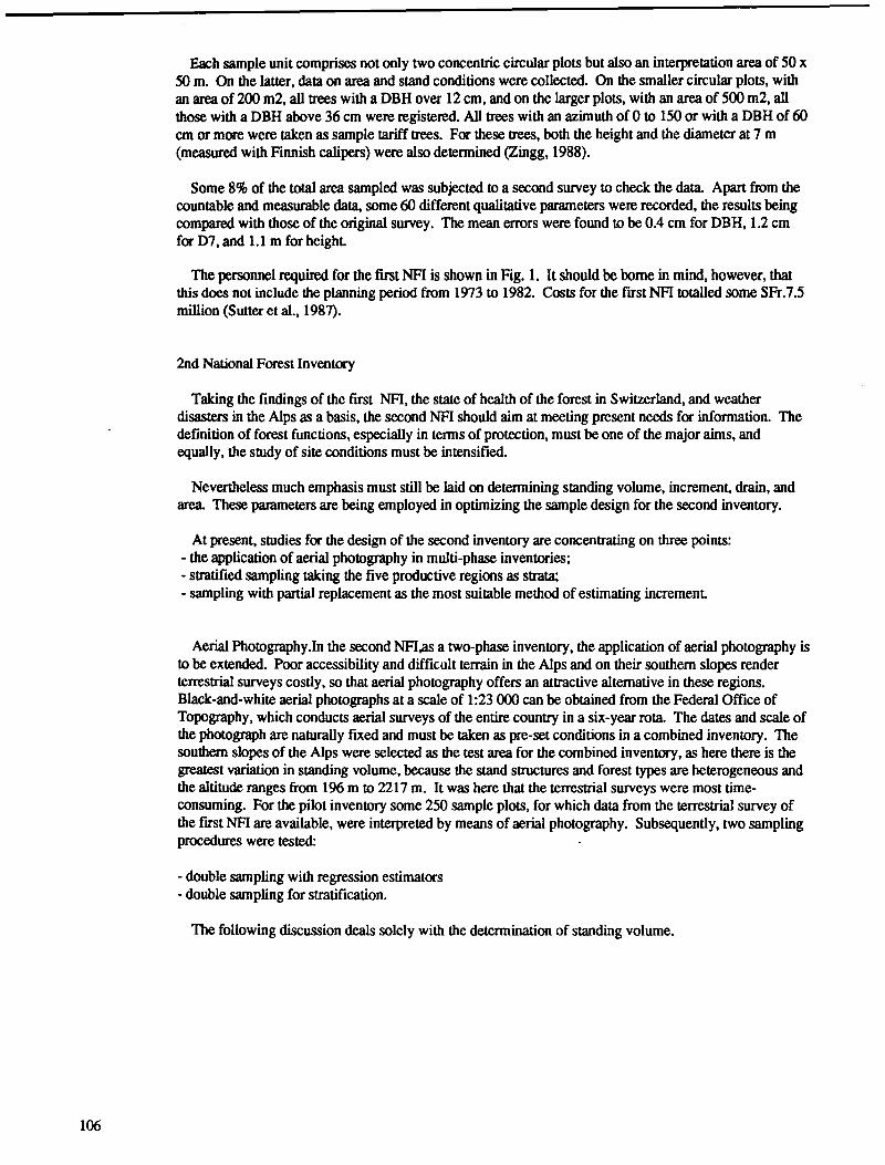
Each sample unit comprises not only two concentric circular plots but also an interpretation area of SO xSO m. On the latter, data on area and stand conditions were collected. On the smaller circular plots, withan area of 200 m2, all trees with a DBH over 12 cm, and on the larger plots, with an area of 500 m2, allthose with a DBH above 36 cm were registered. All trees with an azimuth of 0 to ISO or with a DBH of 60cm or more were taken as sample tariff trees. For these trees, both the height and the diameter at 7 m(measured with Finnish calipers) were also determined (Zingg, 1988).

Some 8% of the total area sampled was subjected to a second survey to check the data. Apart from thecountable and measurable data, some 60 different qualitative parameters were recorded, the results beingcompared with those of the original survey. The mean errors were found to be 0.4 cm for DBH, 1.2 cmfor D7, and 1.1 m for height

The personnel required for the first NFI is shown in Fig. 1. It should be borne in mind, however, thatthis does not include the planning period from 1973 to 1982. Costs for the first NFI totalled some SFr.7.5million (Sutler et al., 1987).

2nd National Forest Inventory

Taking the findings of the first NFI, the state of health of the forest in Switzerland, and weatherdisasters in the Alps as a basis, the second NFI should aim at meeting present needs for information. Thedefinition of forest functions, especially in terms of protection, must be one of the major aims, andequally, the study of site conditions must be intensified.

Nevertheless much emphasis must still be laid on determining standing volume, increment, drain, andarea. These parameters are being employed in optimizing the sample design for the second inventory.

At present, studies for the design of the second inventory are concentrating on three points:- the application of aerial photography in multi-phase inventories;- stratified sampling taking the five productive regions as strata;- sampling with partial replacement as the most suitable method of estimating increment

Aerial Photography .In the second NFI,as a two-phase inventory, the application of aerial photography isto be extended. Poor accessibility and difficult terrain in the Alps and on their southern slopes renderterrestrial surveys costly, so that aerial photography offers an attractive alternative in these regions.Black-and-white aerial photographs at a scale of 1:23 000 can be obtained from the Federal Office ofTopography, which conducts aerial surveys of the entire country in a six-year rota. The dates and scale ofthe photograph are naturally fixed and must be taken as pre-set conditions in a combined inventory. Thesouthern slopes of the Alps were selected as the test area for the combined inventory, as here there is thegreatest variation in standing volume, because the stand structures and forest types are heterogeneous andthe altitude ranges from 196 m to 2217 m. It was here that the terrestrial surveys were most time-consuming. For the pilot inventory some 250 sample plots, for which data from the terrestrial survey ofthe first NFI are available, were interpreted by means of aerial photography. Subsequently, two samplingprocedures were tested:

- double sampling with regression estimators- double sampling for stratification.

The following discussion deals solely with the determination of standing volume.

106

Aer

ial

Pho

to I

nter

pret

atio

n F

ield

Sur

vey

Fig

.l T

ime

Con

sum

ptio

n (M

an Y

ears

)

Double Sampling with Regression Estimators.The first step was to compute a volume function fromparameters measured on the aerial photographs. To this end, the data set was halved and the regressionfor one hah7 calculated. The volume as determined in the terrestrial surveys on the basis of tariff functionswas taken as the dependent variable. The independent variables (tree height as the mean of threemeasurements, crown length as the mean of nine measurements, density of cover, altitude from which thephotograph was taken, cumulative production), all of which can be determined from the photograph, wereemployed to compute two volume functions:

V = f (cumulative production, tree height)V = f (cumulative production, crown length).

These variables also proved significant in separate regression calculations for various forest types,stages of development, mixture proportions, and stand structures, though the multiple R2 was usuallybelow 0.4.

The other half of the data set was employed to compare the volumes determined from the terrestrialsurveys and the aerial photographs. Even for sub-units such as forest type, stage of development, mixtureproportion, stand structure, and degree of cover no significant differences were observed.

Once these regression calculations had been completed, 30 samples with a sample size m, i.e., betweenSO and 200, were simulated at the second level in order to determine the correlation between the variableof interest (terrestrial volume) and the auxiliary variable (volume as computed from aerial photographs).Where the sample size m was smaller than 100, R2 between the individual simulations varied greatly (0.6to 0.05). With 100 samples or more it stabilized between 0.2 and 0.3.

As a last step, the costs for the combined inventory were compared with those of a purely terrestrialsurvey. In the first NFI, it took S16 min. to survey each sample plot on the southern slopes of the Alps.As the costs for the photo-interpretation of one sample plot depend on the number of sample plots perstereo model, the optimum selection had to be done by iteration.

Assuming the standard error for one-phase sampling, the optimization results in a reduction of 7 to 12%in labour, depending on the difficulties of orienting the aerial photograph.

Through optimization given the total expenditure, the combined inventory allowed a reduction in errorof 3% to 4%. In calculating costs, the investments in equipment for interpretation and in programmingwere not taken into account; for the aerial photographs the cost of the copies but not of the actual flightcoverage had to be considered. If the latter were taken into account, a comparison of costs would showthe combined inventory to be disadvantageous.

The results of the pilot inventory do not agree with those of other combined inventories using doublesampling with regression estimators. The main reasons for this are doubtless the difficulties due to thegreat variation in the forest within small areas and the scale of the aerial photographs (1:23000). Atpresent, in order to determine the influence of the accuracy of locating the centres of the two sample plots,the centres of the terrestrial sample plots are being marked so as to be visible on the aerial photographs, sothat the distance between the centres of the terrestrial and aerial sample plots can be established.

Double Sampling for Stratification. As the results of the regression sampling indicated that a combinedinventory is not particularly suitable for determining standing volume in the test area, double sampling forstratification (Johnson, 1982) was investigated as an alternative. Here, instead of taking a parameter fromthe aerial photograph as an auxiliary variable and relating it to the variable of interest through calculatingthe regression, the allocation to a particular stratum was taken as the auxiliary variable.

108

This procedure has been in application in the national inventory of Finland since the 70's (Manila, 1985).In the test area the most suitable basis for stratification was found to be the stage of development. Thiswas classified in five strata: juvenile forest, polewood, young to middle-aged timber, mature timber, andmixed.

In order to determine the variance of the mean for different sample sizes in the second phase, sampleswere simulated, 30 simulations being conducted for each of the sample fractions 0.3,0.5,0.7, and 0.9 perstratum.

Table 1 shows the costs for the various sample fractions. Even with a sample fractions of only 0.7, thecosts as compared with a one-phase inventory can be reduced by about 25%. As this reduction in costsinvolves only a slight increase in standard error (see Table 2), two-phase sampling for stratification mustbe regarded as more suitable than two-phase sampling with regression estimators, and will consequentlybe applied, at least in some parts of Switzerland, in the second NFL

Sampling with Partial Replacement. The main aim of the NFI - large-scale monitoring of changes in theforests of Switzerland - can only be achieved through successive inventories. Consequently the NFI wasdesigned with a view to the establishment of a permanent inventory. All the sample plots surveyed in thefirst NFI - somewhat more than 10 000 in number - were permanently marked so that they could berelocated The centres were marked with aluminium stakes and the sample plot with coloured signs. Foreach tree, the azimuth and distance from the plot centre were recorded. Tree mapping and survey recordswill allow relocation even after several years.

Since (a) permanent and temporary sample plots yield equally accurate figures for standing volume; (b)only permanent sample plots provide direct information on changes in increment; (c) the degree ofaccuracy required in determining increment differs from that for standing volume; and (d) temporarysurvey plots are less expensive to survey than permanent ones, sufficient permanent plots should beavailable to determine increment, and, if necessary, additional temporary plots should be surveyed toguarantee the higher degree of accuracy required for the estimation of standing volume.

The concept of a permanent inventory demands that the permanent sample plots remain representativefor the entire area. To ensure this, and to preclude any influence of management, the exact location of thesample plot centre should not be known to the local foresters. As in the first NFI they understood thesignificance of the coloured markings and the location of the sample plot centres coincided exactly withthe intersections of the grid on the topographical maps, it must be assumed that the location of the sampleplots is known. Further, some 700 sample plots are surveyed each year in forest damage inventories,while a third of the cantons use the NFI sample plots for their own forest damage inventories. In order toverify the representativeness of the results and establish whether any adaptation is necessary, it isabsolutely essential that temporary sample plots be employed in the second NFI, some of which should bepermanently marked for future use in subsequent national inventories or other purposes such as cantonalforest damage inventories.

Both in terms of accuracy and flexibility SPR appears the most suitable method for the second NFI.

Stratification. The aim of stratification is to divide a population into classes in such a way that thevariance within each class is less than that of the population as a whole. Other factors to be consideredinclude working conditions in a given area and different evaluation of the primary variables; for example,in many areas of the Alps the protective function of the forest is considered more important than timberproduction.

Since a stratification based on purely statistical considerations will not be accepted, the existingdivisions within the country must be employed as strata. Beside the cantons, which because of their

109

Tab.lrDouble sampling for stratification: estimated costs

Costs* per field plot: 571 min.Costs'" per photo plotl; 38.3 min

Sample design number of costs(h)field plots

no photo samples 236 2246

double sampling

s.f.= 0.3 71 676

s.f.= 0.5 118 1123

s.f.= 0.7 165 1571

s.f.= 0.9 212 2018

number of total costs(h)photo plots

2246

236 827

236 1274

236 1722

236 2169

* only variable costs1 relative orientation of stereo model

Tab.2 Double sampling for stratification: Costs and standard error.

Sampling design costs (h)

1-phase sampling 2246

double sampling for stratification,sampling fraction:

0.3 827

0.5 1274

0.7 1722

0.9 2169

S.E. cost-difference in rela-tion to 1-phase sampling

8.94

14.58 -63.2%

11.62 -43.3%

9.98 -23.3%

9.07 -3.4%

110

differing size and purely political delimitation are unsuitable as strata, the country has been divided intofive production regions, that have been used in forest statistics for some time. These units allow a roughdetermination of the various conditions for production, which are also reflected in the objectives of thesecond NFL The standing volume in the different regions varies between 176 and 417 m3, while the yieldranges from 0.3% on the southern slopes of the Alps and 2.1% in the Mittelland.

The cumulative production can be employed as a measure for the estimation of increment It is definedas the maximum attainable mean increment per hectare and year under optimum stocking andmanagement It is estimated by means of models based on the site characteristics elevation, exposure,growth region, slope inclination, relief, and acidity of the bedrock.

As regards permanent inventories, there are certain objections to stratified samples:

- where other proportional data sets are employed, the computation of unbiased estimators may becomevery difficult after several surveys because the formulae may become very complicated;- large cantons extending over more than one production region require subdivisions in evaluation;- the production regions are not ideal as strata for all variables;- it is uncertain whether the strata will remain constant in the course of time.

With a view to a flexible inventory design, no pre-stratification is applied. The sample plots are to besystematically surveyed without consideration of the strata limits. For the computation of estimatedvalues, post-stratification is to be used.

Summary

The design of the second Swiss National Forest Inventory will be characterized by the transition from apure determination of current conditions to a permanent inventory permitting the monitoring of changes.

The procedure to be used will be sampling with partial replacement Aerial photography will beapplied not primarily for large-scale surveys but will be concentrated on areas for which information onstanding volume is inadequate or which are difficult of access. The application of double sampling forstratification will allow the subsequent use of satellite data.

A great deal of emphasis is being laid on flexibility of the design. Adaptation for new questions arisingin the inventories of the twenty-first century must be possible and is decisive for the final selection of theinventory method.

LITERATURE

Bachofen H. et al., 1988: Schweizerisches Landesforstinventar, Ergebnisse der Erstaufnahme,EAFV,BerichtNo.305.

Johnson D.C., 1982: Theory and Application of Selected Multilevel Sampling Designs, PhD-Thesis, Colorado State University, Fort Collins, Colorado.

Manila E., 1985: The Combined Use of Systematic Field and Photo Samples in a Large-ScaleForest Inventory in North Finland, Communicationes Instituti Forestalls Fenniae No. 131.

Sutler R. et al., 1987: The Swiss National Forest Inventory, in: FAO/ECE/FINNIDA, ForestResource Assessment Meeting, Kotka, Finland, 26-30 October 1987.

Zingg A., 1988: Schweizerisches Landesforstinventar, Anleitung fuer die Erstaufnahme 1982-1986, EAFV, Bericht No. 304.

Ill

Developing ATLAS Growth ParametersFrom Forest Inventory Plots

John R. MillsResearch Forester

USDA Forest Service, Pacific Northwest Research StationPortland, Oregon 97208

ABSTRACT

The implementation of an age-based stand projection model for the 1989 RPA timberassessment was dependent on the utilization of inventory plot data. The projection mechanism inthe aggregate timberland assessment system (ATLAS) model requires yield tables and stockingadjustment equations to project stand growth. A national inventory database of plot summaryrecords, assembled by the Forest Inventory and Analysis work units of the USDA Forest Service,was the source of data for most model inputs. Techniques were developed to generate yield tablesand stocking adjustment parameters from the growth variables in the database. The techniquesassume the latest forest measurements can be used to project timber stands into the future.Questions remain, however, over using the data beyond its limits. Studies of this kind could beimproved with additional and more consisted resource information.

INTRODUCTION

The aggregate timberland assessment system (ATLAS)1 can simulate growth and harvest for awide range timber types and management conditions. The ATLAS model was implemented to make50-year timber supply projections by the USDA Forest Service in the 1989 resources planning act(RPA) timber assessment (U.S. Department of Agriculture 1989). The RPA objective is to compilea comprehensive assessment of the current and future National timber situation. This task requiredmodeling growth and harvest on 344 million acres of privately owned commercial timberland. TheATLAS model was developed to replace TRAS (Larson and Goforth 1974), the timber model usedfor previous assessments. In the RPA modeling process, ATLAS was linked to the economic modelTAMM (Adams and Haynes 1980). The resulting projections of timber inventories, harvests,stumpage prices, wood products consumption and production, and employment in the forest productssector were the result of interaction between biological and economic assumptions and the ensuingequilibrium between the timber supply and the demand for stumpage.

The timber side of this process begins with a periodic inventory of the private timberland in theUnites States conducted regionally by various Forest Inventory and Analysis (FLA) projects of theUSDA Forest Service. The inventory system is designed to collect resource data from a state-levelconfiguration of permanent plots on a 5- to 12-year cycle. To provide resource information for thethis and subsequent Assessments, an RPA timber database was developed to includes 124,000records representing approximately 483 million acres of available timberland (Waddell and Oswald1986). This database proved crucial to the development of both the beginning inventory andprojection parameters input into the ATLAS model. Database plot records included variables forstate, ownership group, forest type, age class (for most plots), site productivity class, net growth, netvolume, and plot expansion factors. Public land is included in the database, however, only data fromplots on privately owned lands were included in the modeling process.

Three categories of input are required to make ATLAS timber projections. The first is agrowing stock inventory that consists of acres and volume per acre by age class. The second is yieldtables and growth parameters used in the projection mechanism. And third is harvest volume. The

Mills, J.R. and Kincaid, J.C., [in preparation]: The aggregate timberland assessment systemLAS): a comprehensive timber projection model.(ATLAS): a com

112

harvest request volume is determined exogenously, for RPA projections TAMM calculated a harvestrequest based on the demand for forest products. (A fourth category of input required for the RPAwas projections of land area by forest type. Projections of forest type transition were supplied byAlig and others [U.S. Department of Agriculture 1989].)

The options in ATLAS allow for harvested acres to get regenerated or leave the managementunit. Area change options allow acres to change ownership, type, or management level. A detaileddescription of the harvest mechanism or area change options is beyond d the scope of this paper.

METHODS

For the purpose of the RPA timber projections, the continental U.S. was subdivided into 8timber supply regions. Within each region, commercial timberland was identified by ownership,forest type, and site productivity class. These identifiers were the key variables used to sort andaggregate the growing stock inventory into management units. The management units represented 2owner groups (forest industry and nonindustrial private), up to 9 forest types (per region), and 3 siteproductivity classes were carried for the Southeast, the South Central, and the Pacific NorthwestDouglas-fir subregion. Within each management unit, growing stock is represented by an array ofacres and volume per acre for 18 age classes (5-years per class in the South, 10-years elsewhere).Options allow for a stratification of the acres and volume within a management unit among 5different management intensities. Each management intensity has growth parameters to model aresponse to a particular condition or treatment (custodial management, thinning, fertilization, geneticimprovements, etc.). In the RPA timber projections, 249 management units were developed, 84management units had more than one management intensity.

The model inputs for beginning inventories were either developed by the FIA units themselves,as was done in the North Central and South, or developed directly from the plot-level information inthe RPA timber database. In either case, the starting area and volume was derived from FIA plotdata.

Projecting Inventory Volume

The ATLAS projection methodology is built around the use of yield tables to project standdynamics. Projections are for periods, the period length is consistent with the years in an age class.A stocking adjustment equation is the dynamic link between the existing timber inventory and theyield table. Stocking is growing stock volume divided by yield table volume. The stockingadjustment is based on the approach-to-normal concept, that is, over time stand density will naturallytrend towards that of the normal undisturbed condition for that particular forest type and site (seeChaiken 1939, Gevorkiantz and Duerr 1938, Schumacher and Coile 1960). Growth is the volumechange that results when acres are projected to the next oldest age class. A system similar to thiswas described by Chapman (1924) as a technique to employ a normal yield table to predict futurevolume for less than normal stands. Normal yield tables have typically not been used in ATLAS, itcan be said the yield table acts as a volume "guide curve" rather than a volume asymptote. Insteadof the term approach-to-normal, Leary and Smith (in press) use the term "relative density change" todescribe this mechanism. The calculation of stocking within a single age class, its adjustment, andthe subsequent change in volume can be represented as

113

S» = VY,when Y, > 0 and i > 0 , (1)

w, = b« + b*s« ' °r (2>S|+i,t+i = SH + b,Sj, + b2S „when b, > 0 and b2 < 0 , and (3)

whereS = stocking ratio,V = growing stock volume per acre,Y = yield table volume per acre,i = age class,t = projection period, andb,,bz = stocking adjustment coefficients.

Equation (1) calculates the stocking ratio in the current period. Equations (2) and (3) are two formsof the equation used to calculate the approach-to-normal stocking adjustment. Equation (2) is alinear form derived from McArdle and others (1961). Equation (3) is a quadratic form derived byGevorkiantz and Duerr (1938) and implemented in the North Central region by Leary and Smith (inpress). Equation (4) represents the calculation of volume next period, acres associated with V havebeen assigned to the next highest age class. To define this single age class more specifically in anATLAS inventory, subscripts could be added to represent management intensity, and managementunit (b, and ba would not be subscripted by management intensity). Regenerated acres are assigneda beginning stocking ratio developed exogenously (discussed later).

The following formulation represents the summation of regular growth reported for period 't'within a single management intensity:

TRG,= S V l+1>t+1 - VN ; (5)i-O

where TRG equals the total regular growth per acre calculated under one base yield table, n equalsthe highest age class. Total growth and total volume are the product of acres their and associatedvolumes per acre.

Developing Yield Tables

There were 422 yield tables used in the timber projections. They came from three sources:other models; earlier studies; and derived from plot data. As a model input, yield tables are atabular representation of net volume per acre for 18 age classes. A difficulty encountered in theRPA was that published yield tables representing broad forest types rarely exist. Therefore, yieldtables were developed to represent the various type-site-management aggregations. Most of the yieldtables were not ownership specific, instead, growth differences between the two owners was reflectedin the stocking adjustment mechanism and the regeneration stocking ratios.

Fully stocked yield tables were developed to represent the Southeast and South Central regionsin the fourth forest study (U.S. Department of Agriculture 1988) (a predecessor of ATLAS; TRIM[Tedder and others 1987] was the timber projection model for the fourth forest study). These yieldswere derived from survey plot data that was screened to include only plots with enough growingstock to be classified as fully stocked by FLA standards (see McClure and Knight 1984). For theseplots, the average net volume was calculated by type, site class, and age class (5-year). Curves werefitted to the averages for each type and site to create a smooth volume by age relationship. I would

114

expect the yield volumes to range somewhere between classical empirical yield table volumes (anaverage volume calculated from all plots), and normal yield table volumes (calculated fromundisturbed plots with normal stocking). Implementation of these yields for the RPA requiredrecalibration of the stocking adjustment parameters.

The yields developed to project the Northeast, the Rocky Mountains, the Pacific Southwest, thePacific Northwest Ponderosa Pine subregion.and several types in the Pacific Northwest Douglas-firsubregion were developed using growth data from the plots in the RPA timber database. In anearlier study I referred to yields derived from plot growth data as growth yields (Mills 1989).Growth yields were developed using all plots of the specific forest type (and site-when represented).An average growth per acre was calculated for each age class. Linear regression was used to smoothvariation over the age classes and to predict growth for age classes containing no data. A yield tablewas developed by cumulating the average growth per acre over all 18 age classes. The valuecorresponding to each age class in the resulting table represents the summation of the average netgrowth up to and including the current age class.

The logic of growth yield tables is, at the regional level of aggregation a cross section of growthis an indicator of the average volume change and hence, makes a representative volume guide curve.The slope of fully stocked empirical yield curves tends to flatten in the older age classes, and this isoften interpreted to indicate little or no net growth occurs in older stands. The plot growthassociated with older stands, however, is often higher would be expected from the slope of fullystocked yields. The growth on older stands is built into the growth yield tables, making themcompatible with the ATLAS "volume guide" role of yield tables.

The Calculation of Stocking

There are two types of inputs associated with stocking that were developed from the database.One is the parameters (b, and b2) associated with equations 2 and 3, the other is a regenerationstocking ratio.

The parameters in equation 2 were calculated for all types and sites represented in theNortheast, Rocky Mountain, Pacific Southwest, and Ponderosa Pine Subregion of the PacificNorthwest. Elsewhere they were calculated selectively based on performance review of b, = 0.1 andb2 = 0.9; these values asymptotically increment stocking to 1.00 . Equation 3 was used only in theNorth Central region.2

The parameters in equation 2 were estimated by owner and type (and site when enough plotsexisted). The procedure required the yield table, the plot volume per acre, and the annual growthassociated with the plot (based on remeasurement). An estimate of plot volume was calculated forage = i-1 by subtracting net growth from net volume at age = i. A stocking ratio was thencalculated for the plot volume at age = i (as in equation 1), and also for the estimate of volume atage = i-1 as shown below:

EVM = V, - G,L , and (6)

ESM = EVM / YM ; (7)

wherei = age classEV = estimated volume per acreES = estimated stockingG = annual growth per acre, andL = number of years per age class.

2For further information contact Rolfe Leary, North Central Forest Experiment Station, 1992Folwell Ave., St. Paul, MN 55108

115

After screening the set of stocking ratios for outliers, liner regression was used to estimate b, and bzfrom the equation

S, = b, + b2ESM . (8)

Most regressions were run with at least 100 observations.

The regeneration stocking ratio is simply SN for all t when i = 0, it represents the averagestocking of the regenerated inventory associated with the yield table. For most yield tables the ratiowas calculated from the inventory plot volume associated with the yield table. Average stocking wascalculated for each age class and then acre weighted between age classes. This technique assumesregeneration will start at average stocking based on the inventory within the management unit(calculated when t = 0). After regeneration, stocking will trend towards the stocking asymptote. Inthe case when yield tables were developed to represent realized volume (i.e. under specificmanagement regimes), the regeneration stocking ratios were 1.0 or 0.9 and the stocking asymptoteswere 1.0 (the yield table).

The Assignment of Plot Age

In two regions the age variable was missing from approximately half of the plots. In both theNortheast and South Central regions, plots were not assigned a stand age because either the sampledstands were unevenaged, or the plot straddled two distinct forest conditions. In either case, plot agewas not assigned because of differences in species, size, and age within the sample. Age is arequired variable because it determines the initial starting point of acres in the volume projectionmechanism. To estimate age for these plots, two age estimation techniques were employed. For theSouth Central region, researchers at the USDA Forest Service, Southern Forest Experiment Station(Starkville, MS) used yield tables and stocking variables to assign age based on plot volume andstocking. On Northeast plots that did have an assigned age, volume and age were poorly correlated.The assignment of age using yield table volume would seriously have truncated the distribution ofacres by age class. To estimate the ages of these plots, I employed linear regression on variablessuch as stocking, site, average diameter, volume, and growth to developed estimation equations forplots with age (by forest type). These equations were then used to estimate the age of theindeterminant-age plots. Yield tables for the Northeast were developed from all plots after theassignment of age.

DISCUSSION

Many positive things should be said of overall RPA modeling effort. The communication withFIA units was good, the plot-level database was a new improvement, and the evaluation andcomment received from reviewers was excellent. The extensive use of plot data for the developmentof growth and yield parameters made possible the Nationwide implementation of ATLAS. The RPAdatabase was an essential tool; without which, given the timeframe and budgets, inputs for theNortheast and Rocky Mountain regions would not have been constructed. (An alternative for thesetwo regions was to use the TRAS model with 10-year old input files.)

Data from permanent plots allows for a calculation and projection of change over time. If thelatest measurements are considered the best evidence of what is happening in the field, then the useof growth data to calculate yield tables and density change parameters is consistent with our desireto project a future based on current observation. Not discussed here was the attempt to modelassumptions of improvements in timber management. Several management intensities weredeveloped to represent the expected returns from enrolling acres into intensive managementschedules. The intensified management yield tables were either developed from models or based onother yield tables. The yield tables and acreage enrollment rates were subject to extensive review.

116

Several questions arose in the analysis and it is not clear how the answers would effect theresults. Does a cross section of average growth really represent the potential for individual stands,or in this case, an aggregation of plots? If the values in a growth yield table are independentbetween age classes, then is this kind of yield table accurate for plot projections? The correlation ofplot age with plot volume and growth might also be questioned. From the plot data there was noway to be sure how well the growth variable was correlated with the age variable. Disturbance orpartial harvest of a plot could conceivably reduce the average age of a plot and the net plot growthmight not be representative of the residual stand. A good correlation is important for the growthyield tables and stocking adjustment parameters. It is also not known what bias might have beenintroduced by the assignment of age to plots. Should the same technique be used to project both atrue uneven age plot and a plot that straddles two different conditions? The answers to thesequestions are the subject of further study.

As good as the database was, there are some problems at the National level that are rooted inthe FIA procedures themselves. Generally, there is a lack of consistency in the inventory techniquesbetween FIA regions. The plot design, sampling intensity, inventory cycle, the calculation of growth,and the estimate of harvest vary by region. In many cases techniques have been tailored toparticular local conditions and user requirements, in other cases the differences are based ontradition.

The Future

Preliminary work has already begun, the draft projections for the 1993 Assessment Update willbe made in the summer of 1992. In the interim, there is time to make modest improvements. It hasprobably been said at the end of every study of this kind, a better job could be done with additionaldata. Any model used across such a large area will face many of the same data challenges. A list ofdesirable variables to incorporate in the next RPA database would include: (1) a disturbance codeassociated with the plot to indicate previous damage or harvest, (2) sample kind--to indicate aremeasured or newly established plot, and (3) age, volume, and growth estimated at time of previoussurvey. The historical information would allow for screening of plots that might exhibit growth thatis not necessarily attributed to age or current volume. It would lead to finer calibration of thedensity change parameters, and in addition, provide data for the effort to improve the representationof harvest.

The assignment of age will be a recurring challenge for both uneven-aged stands and plots thatstraddle two distinct conditions. It has been proposed that an unevenaged projection system bedeveloped for the Northeast. As the modeling process evolves to a finer level of resolution, a plotstraddling two conditions will present a more difficult challenge.

If we keep in mind our purpose and our users, this modeling process will continue to evolve.New ideas translate into new models, additional validation and calibration, and there is always desirefor "better" data. The projections for the 1989 timber assessment are finished, but the techniquesand results of the whole process, from data collection through modeling, will be the topic livelydiscussion for years to come.

117

REFERENCES

Adams, Darius M.; Haynes, Richard W. 1980. The 1980 softwood timber assessment marketmodel: structure, projections, and policy simulations. Forest Science Monograph 22. 64 p.

Chaiken, L.E. 1939. The approach of loblolly and Virginia pine stands toward normal stocking.Journal of Forestry. 37: 866-871.

Chapman, Herman Haupt. 1924. Forest mensuration. New York: John Wiley & Sons. 557 p.

Gevorkiantz, S.R.; Duerr, William A. 1938. Methods of predicting growth of forest stands in theforest survey of the Lake States. Economic Notes No. 9. St. Paul, MN: U.S. Department ofAgriculture Forest Service, Lake States Forest Experiment Station. 59 p.

Knight, Herbert A.; McClure, Joe P. 1975. North Carolina's timber, 1974. Resour. Bull. SE-33.Asheville, NC: U.S. Department of Agriculture, Forest Service, Southeastern Forest ExperimentStation. 52 p.

Larson, R.W.; Goforth, M.H. 1974. TRAS: a timber volume projection model. Tech. Bull 1508.Washington, DC: U.S. Department of Agriculture, Forest Service. 15 p. • • •„. «

Leary, Rolfe A.; Smith, W. Brad, [in press] Test of the TRIM inventory projection methods onWisconsin jack pine. Can. J. For. Res. 20: .

McArdle, Richard E.; Meyer, Walter H.; Bruce, Donald. 1961. The yield of Douglas-fir in thePacific Northwest. Tech. Bui. No. 201. Washington, DC: U.S. Department of Agriculture, ForestService. 74 p.

McClure, Joe P.; Knight, Herbert A. 1984. Empirical yields of timber and forest biomass in theSoutheast. Res. Pap. SE-245. Asheville, NC: U.S. Department of Agriculture, Forest Service,Southeastern Forest Experiment Station. 75 p.

Mills, John R. 1989. TRIM timber projections: an evaluation based on forest inventory^ ;measurements. Res. Pap. PNW-RP-408. Portland, OR: U.S. Department of Agriculture, ForestService, Pacific Northwest Research Station. 27 p. .

Schumacher, F.X.; Coile, T.S. 1960. Growth and yields of natural stands of the southern pines.Durham, NC: T.S. Coile, Inc. 115 p. . , ;

Tedder, P.L.; La Mont, Richard N.; Kincaid, Jonna C. 1987. The timber resource inventorymodel (TRIM): a projection model for timber supply and policy analysis. Gen. Tech. Rep. PNW-202.Portland, OR: U.S. Department of Agriculture Forest Service, Pacific Northwest Research Station.82 p.

U.S. Department of Agriculture. 1989. An analysis of the timber,situation in the United States:1989--2040, parts I and II. Review Draft. Washington, DC: U.S. Department of Agriculture, ForestService. , , : .

U.S. Department of Agriculture. 1988. The South's fourth forest: alternatives for the future. For.Resour. Rep. 24. Washington, DC: U.S. Department of Agriculture, Forest Service. 512 p.

Waddell, Karen; Oswald, Daniel. 1986. The National RPA timber database, 1990 RPA timberassessment data dictionary. Portland, OR: U.S. Department of Agriculture, Forest Service, PacificNorthwest Research Station. 65 p. On file with: Forest Inventory and Analysis Project, ForestrySciences Laboratory, Pacific Northwest Research Station, P.O. Box 3890, Portland, OR 97208-3890.

118

Forest Change - An Assessment ofNationwide Forest Inventory Methods

Richard BirdseyForest Service - USDA

Washington, DC 20090-6090

Hans SchreuderForest Service - USDA

Fort Collins, CO 80526-2098

ABSTRACT

Forest Service Forest Inventory and Analysis (FIA) projects have developed several philosophiesand techniques to estimate growth, removals, and mortality in different situations. Regional methodsare related to past and current sampling designs and plot configurations, time between successiveinventories, and regional characteristics of forest resources. Since FIA surveys involve an extensivenetwork of permanent sample plots, some remeasured for more than 30 years, the data has uniquevalue for long-term monitoring of forest conditions at the national level. Adoption of some newinventory techniques could improve regional and temporal consistency and enhance the usefulness ofthe data for monitoring purposes.

INTRODUCTION

This assessment is a summary of background material prepared for an internal review of ForestInventory and Analysis (FIA) methods for assessing forest change. In the past, information from thenationwide forest survey was typically used to assess the adequacy of the nation's timber supply.Although timber supply is still an important issue, the public is demanding more information aboutcurrent and prospective changes in forest resources. Increasingly, FIA is asked to provide non-traditional information such as the amount of carbon stored and accumulating in U.S. forests, or theeffects of atmospheric pollutants on forest growth. In addition to traditional requests from forestindustries and other timber interests for information about timber supplies, FIA has recently beengetting requests for information related to environmental issues from the Environmental ProtectionAgency, the American Forestry Association, the President's Council of Economic Advisors, and theMan and the Biosphere Program, to name a few.

Our challenge is to make the-best use of existing long-term data sets for answering newquestions, and to develop better ways to meet these and future information needs. The basic inventorydesign was developed in the 1950's to provide efficient estimates of timber volume and forestcondition. If current methods are inadequate or inefficient for meeting new information needs, thenprocedures will be revised in ways that maintain the strength of long-term continuity.

119

A BRIEF HISTORY OF FOREST INVENTORY METHODS

The systematic survey of U.S. forests was begun in 1930 under the authority of the McSweeney-McNary Forest Research Act of 1928. Sample surveys were made by what was known as the line-plotmethod (Hasel 1938; Robertson 1927). Parallel survey lines at fixed intervals were run at approximateright angles to the prevailing drainages. Quarter-acre sample plots were established at each 10-chaininterval (660 feet) along the survey lines by field crews that literally walked from one end of a state tothe other (Eldredge 1934). This design was used for most of the U.S. until about 1950, except duringWorld War II when no surveys were conducted.

Of all the decades since the forest survey began, the 1950's had the most sweeping and lastingchanges in inventory methods. During that decade, inventory projects in different regions begandeveloping and applying new inventory designs based on advances in forest sampling theory and thewidespread availability and use of aerial photography after the war (Hasel 1954). Cruise lines werelargely abandoned in favor of permanent sample plots located in a systematic way. Information fromaerial photos was used for stratification and plot location. The statistical technique of double samplingfrom aerial photographs was an important advance that is still widely applied today (Bickford 1952).

The plotless or variable-radius plot method of timber cruising, discovered by Walter Bitterlich,was introduced to the U.S. during the 1950's by Lew Grosenbaugh (Bitterlich 1948; Grosenbaugh1952a, 1952b, 1958). Horizontal point sampling became generally accepted as a more efficient methodfor selecting sample trees for volume estimation. Inventory projects replaced fixed-radius sample plotswith variable-radius sample plots. Various basal area factors and plot configurations were used. Forexample, in the South, pairs of 1/4 acre fixed-radius plots were initially replaced by pairs of variable-radius plots selected with a prism basal area factor of 10. But by the 1964 survey of Louisiana, the plotpairs established at each sample location were replaced by a cluster of 10 variable-radius plots selectedwith a prism basal area factor of 37.5, and supplemented with 3 small fixed-radius plots for samplingtrees less than 5.0 inches in diameter at breast height (dbh). Similar changes were occurring at all theinventory projects across the country.

The establishment and remeasurement of permanent sample locations became popular during the1950's under the label Continuous Forest Inventory (CFI). Permanent plots were seen as the answer toproblems in estimating growth, removals, and mortality from temporary plots. Permanent plots werecontroversial, though, since higher establishment and marking costs made permanent plots moreexpensive than temporary plots for estimating all of the other information upon which decisions aboutactual forestry operations were based (Grosenbaugh 1959).

Despite the controversy, permanent, well-hidden sample plots became the norm across the U.S.Many of these same plot locations are still remeasured periodically, some for the fourth time. In theEast, sample plots were located at the intersections of grid lines or at random locations selected from asystematic grid. In the West, mapping of forest areas and stratification from aerial photographs wereused more frequently, often in combination with a double sampling design.

During the 1960's and 1970's, survey designs became increasingly diverse and complex.Sampling with partial replacement was developed as an efficient way to select an optimum mix ofpermanent and temporary plots (Ware and Cunia 1962). Advanced multi-stage and multi-phasesampling designs were developed to take advantage of new techniques in remote sensing. Differentcombinations of techniques were found suitable for each forest survey region. Many of thesedevelopments are evident in the survey designs currently used, but none has replaced double samplingfrom aerial photographs and permanent sample plots as the mainstay of the U.S. forest inventorydesign (U.S. Forest Service 1987).

120

OVERVIEW OF CURRENT FOREST INVENTORY METHODS

Inventory Objectives

Timber supply and environmental issues of the 1980's require good trend information and datafor use in many kinds of models, in addition to the more traditional estimates of current conditions.Issues have increasingly involved detailed analyses of estimates from successive inventories. Arecurring problem has been to determine whether observed trends are real or artifacts of changes ininventory and sampling design, and whether observed trends represent a departure from what is normalor expected. An elusive goal has been a credible statement about the causes of observed trends usingperiodic inventory data.

Sampling Design

Most FIA units use two-phase sampling for regular forest inventories. The first phase consists ofa large number of sample points selected on aerial photographs and classified by a photo interpreter as,at minimum, forest and nonforest. The photo samples may also be classified by volume class, foresttype, or disturbance. The second phase consists of smaller number of sample points selected on theaerial photograph and visited in the field. The field classification is typically used to correct for photo-plot misclassifications due to out-of-date photography or interpreter error. The sample points of phasetwo comprise the locations of permanent and temporary field plots used to estimate volume, growth,removals, mortality, and other forest inventory parameters, and to classify sample plots by ownership,forest type and other vegetation or site characteristics.

Typical variations among FIA projects involve the degree of dependence between phase one andphase two, the use of subsampling in either phase, the specific sampling rules used to select samplelocations, and the sampling intensity. These variations affect the precision of estimates and theefficiency with which an inventory is conducted, but do not lead to any known bias in results.

Selection of Sample Trees

Sample trees are selected in clusters of fixed- and variable-radius sample plots at permanent andtemporary locations. The vast majority of plot locations are now permanent. Generally, fixed-radiussample plots are used to select small trees (less than 5.0 in. dbh) or very large sample trees (greaterthan 35.0 in. dbh), while variable-radius plots are used to select other trees. From 4 to 10 samplepoints are arranged in a specified configuration to cover an area from 1 to 5 acres.

All FIA units rotate satellite sample points into a forest classification if the central or primarysample point is classified as forest. However, one significant difference among FIA units is thetreatment of sample plots that straddle different forest conditions. Some projects move sample pointswithin a cluster into the same forest condition, while other projects let the points stay where theyoriginally fall.

121

Individual Tree Measurements

Individual tree measurements fall into 3 categories: those made for every sample tree, thosemade for a subsample of all sample trees, and those made for an independent sample of trees.Measurements made on subsamples or independent samples are usually used to develop models andestimate parameters that are applied to all sample trees. Examples are volume regressions, biomassregressions, diameter growth models, height equations, and utilization factors. In all cases the intent ofthe models is to relate something that is difficult or time-consuming to measure (such as volume) tovariables that are relatively easy to measure over a large sample (such as dbh).

In general, every sample tree in the U.S. is identified for species and measured for dbh. Mosthave at least one length (or height) measurement. All sample trees are classified as growing stock orcull and assessed for damage. Depending on the region, additional measurements may be made,including section lengths, upper stem diameters, stump heights and diameters, cull deductions, and logor tree grade. Sometimes models are used to predict individual tree measurements that are missing ornot made for every sample tree.

Standing or felled trees on subsample and independent sample plots may be measured in greatdetail and accuracy. Procedures and measurements vary by region and are usually adapted to localconditions and knowledge.

Tree Volume Estimation

Individual sample tree volumes may be estimated directly by detailed measurement of everysample tree, or by using a regression model with relatively simple and accurate tree measurements asindependent variables. Estimates of volume growth are usually based on repeated volume estimates ofsample trees surviving from one inventory to the next, or for new sample plots, estimates of volumeincrement derived from tree ring measurements or growth models. Estimates of mortality volumes areusually derived from past measurements of sample trees on remeasured plots and tree measurements atthe second inventory that reflect tree dimensions at time of death. Estimates of removal volumes fromsample plots are usually derived from past tree measurements on remeasured plots, and application ofgrowth models to predict dbh and/or length at the time of removal.

Definitions and Estimators

National consistency is maintained through standard definitions of key terminology and variables.Certain estimation details may not be defined nationally. This is because specific inventory proceduresare developed locally in order to make the best use of available sources of data, to be consistent withlocal data needs and standards, and to make the best use of local knowledge developed through manyyears of research.

Similarly, estimators are not prescribed nationally because they are always dependent on thesampling design, methods used to select sample trees, and availability of necessary models. In generalthe entire inventory system is adapted as well as possible to local conditions in order to achieveefficiency while serving local as well as national data needs.

The principal estimators of forest change are growth, removals, and mortality. These variablesare defined as either average annual estimates for the intersurvey period, or current annual estimates.The second.definition implies that successive inventory estimates are not linked, although permanentsample plots may still be remeasured to estimate growth, removals, and mortality. Current estimatesare used when it is necessary to make all of the inventory estimates apply to a single point in time.Current estimates are generally preferred when the period between inventories is lengthy, when there

122

have been significant changes in definitions or methods that make successive inventories incompatible,or,when one of .the estimates is derived from a different survey method .such as a census of timberremovals by forest industry. Estimates of periodic averages have become more common in recent yearsas the survey interval has shortened, improvements in data processing capabilities have allowed . .•extensive recomputation of past surveys to account for procedural changes, and estimates of removalsfrom sample plots rather than industry surveys have become more commonplace.

Classification Variables

All forest inventory projects collect and compile classification data used to post-stratify sampleplots, for analysis, and screening. Examples of classifications are ownership, forest type, stand-sizeclass, and stand age. Most classification variables have uniform national definitions, but definitionschange over time, and the actual procedures to classify a sample plot may vary over time or fromregion to region.

Sample plot classifications are often derived from basic tree measurements, so the classificationis dependent on the methods used to select sample trees. Sample plot design and rules for rotatingsample points can therefore affect any plot classification, such as forest type or basal area,,that isdependent on tree measurements. So changes in sample plot design and sampling rules can affectsample plot classifications in indirect ways.

USE OF FIA DATA FOR TREND ANALYSIS

FIA inventories represent one of the few sources of long-term measurement data, and the onlycomprehensive network of samples that truly represent forest conditions across most of the U.S. Otherlong:term data .sets such as used in growth and yield studies typically cover selected forest types ormanagement conditions, whereas FIA inventories cover all timberland regardless of location, condition,or management activity. 4 .

Despite the unique, comprehensive nature of the FIA sample network, it has been difficult forsome researchers to accept FIA data as a source of valid trend information (Stout 1989). Part of theproblem is a failure to correctly visualize inventory data as a repeated, natural experiment, and part isdue to the lack of strict temporal consistency in inventory methods.

( Diamond (1983) described 3 kinds of experimental approaches to ecological problems:laboratory,, field, and natural experiments. In laboratory experiments the values of independentvariables'can be controlled, but ecological systems are usually so complex and variable over time thatlaboratory experiments are unrealistically simplistic. Field experiments can incorporate much of thenatural variability of site and climate, but the experimenter can control only one or a few variablesrelated to site or species, often at great cost. In a natural experiment, much control over independentvariables is lost, leaving the experimenter with only site selection as a method of control. The goal of anatural experiment is to select sites as identical as possible in all factors except the one of interest. Themajor advantages of natural experiments are that a large amount of data can be gathered quickly andinexpensively, problems that cannot be created experimentally can be addressed, and problemsinvolving large areas and the end results of long evolutionary processes can be studied. The majordisadvantage is that with limited control of independent variables the experimenter is less sure that anoutcome is 'the result of the specified factor or some unknown factor.

Most analyses of inventory results involve comparisons with the previous survey, and a }

conscientious analyst will diligently account for any changes in definitions or procedures. To fullyanalyze trends in growth or mortality, the analyst must reach back two inventories to establish initialconditions or screen data for consistent populations. Since 3 inventories typically span 20 or more

123

years, the likelihood of changes in procedures and definitions affecting sample plot classifications ishigh. The analyst may need to spend considerable time and effort recomputing survey estimates fromoriginal data to effectively compensate for these changes.

Once a consistent set of data has been assembled, sample plots can be selected to control theeffects of key variables for the two periods. In a cross-sectional study that related forest growth tosulfate deposition, Shifley (1987) selected sample locations from a large pool of inventory plots along asulfate gradient and controlled the effects of growth variation due to stand age, site index, and standdensity for 5 different forest types. This method of experimental control is also appropriate fortemporal analysis of growth trends if the selection variables are strictly consistent.

CAN WE MEET FUTURE INFORMATION NEEDS?

For forest inventory, "acid rain", "global climate change", "forest decline" and "monitoring" arerepresentative concerns of the 1980's. As foresters we are particularly interested in the future and howforests will change in response to long-term environmental changes, and what the potential of forestsmay be to mitigate the effects of anticipated changes.

To address these issues will require an ability to separate expected forest changes due to naturalprocesses, timber harvest, and management, from unexpected changes due to anthropogenicenvironmental changes. We can anticipate a future need to look back at today's data to establishbaseline information for evaluation of future forest conditions.

The national forest inventory needs a strengthened core of basic data elements that are accuratelymeasured in a consistent way to effectively analyze future forest changes. Sample plot classificationsshould be derived from basic measurements that are repeatable over time by different field crews. Thesampling methods must also have temporal consistency because a plot classification may change underdifferent sampling rules. We must be careful about making changes to achieve spatial consistency thatcause basic data to be incompatible with the past or the future.

So when we think about changing sample plot designs or methods of classifying sample plots, weshould always consider how this will affect the usefulness of the data 20 or 60 years from now. Theinventory methods developed in the 1950's, and still in place today as the core of the nationalinventory, represent our basis for analyzing long-term forest changes. Will an analyst from 2020 curseus because we changed something to be more efficient or use a more up-to-date technique? If we areright in anticipating that long-term environmental considerations are of immediate and future concern,then it might be wise to remember temporal consistency when contemplating a state-of-the-art changein inventory procedures.

124

REFERENCES

Bickford, C.A., 1952: The sampling design used in the forest survey of the Northeast. J. For.50: 290-293.

Bitterlich, W., 1948: Die winkelzahlprobe. Allgemeine Forst-und Holzwirtschaftliche Zeitung59(1/2): 4-5.

Diamond, J.M., 1983: Laboratory, field, and natural experiments. Nature 304: 586-587.

Eldredge, I.F., 1934: The forest survey in the South. Forest Survey Release No. 1. NewOrleans, LA: U.S. Department of Agriculture, Forest Service, Southern Forest Experiment Station,5 p.

Grosenbaugh, L.R., 1952a: Plotless timber estimates — new, fast, easy. J. For. 50: 32-37.

Grosenbaugh, L.R., 1952b: Shortcuts for cruisers and sealers. Occasional Paper 126. NewOrleans, LA: U.S. Department of Agriculture, Forest Service, Southern Forest Experiment Station,24 p.

Grosenbaugh, L.R., 1958: Point-sampling and line-sampling: probability theory, geometricimplications, synthesis. Occasional paper 160. New Orleans, LA: U.S. Department of Agriculture,Forest Service, Southern Forest Experiment Station, 34 p.

Grosenbaugh, L.R., 1959: Should continuity dominate forest inventories? Paper presented atshort course on Continuous Inventory Control in Forest Management, U. of Georgia, May 4-8. 13p.

Hasel, A.A., 1938: Sampling error in timber surveys. J. of Agric. Res. 57(10): 713-736.

Hasel, Austin A., 1954: Problems in forest inventory: from the statistical point of view. InStatistics and Mathematics in Biology, Ed. by Kempthorne et. al. Ames, Iowa: The Iowa State CollegePress. 263-272.

Robertson, W.M., 1927: The line-plot system, its use and application. J. For. 25: 157-163.

Shifley, S.R., 1987: Analysis and modelling of forest growth trends along a sulfate depositiongradient in the north central United States. In proceedings, Forest Growth Modelling and Prediction,Ed. by Ek et. al., Minneapolis, MN: Society of American Foresters, 506-513.

Stout, B.B., 1989: Forest decline and acidic deposition - a commentary. Ecology 70(1): 11-14.

U.S. Forest Service, 1987: Forest Service Resource Inventory: An Overview. Washington, DC:U.S. Department of Agriculture, Forest Service, 29 p.

Ware, K.D. and Cunia, T., 1962: Continuous forest inventory with partial replacement ofsamples. For. Sci. Monograph 3, 40 p.

125

Fixed-Versus Variable-Radius Plots for Change Estimation

Charles T. Scott, Research ForesterJames Alegria, Forester

USDA Forest ServiceNortheastern Forest Experiment Station5 Radnor Corporate Center, Suite 200

Radnor, PA 19087

ABSTRACT

Much forestry literature has focused on fixed-area versus variable-radius plots forestimation of current forest characteristics. Variable-radius samples were found to be mostefficient for current basal area and volume estimates, but much controversy arose over theirefficiency for change estimation. As an empirical test of the cost effectiveness of each method,14.8-ft plots were compared with 26.5-ft2/ac BAF (basal area factor) plots. Each pair wasremeasured after 12-13 years and detailed cost measurements recorded for all aspects of thesurvey. With the exception of removals, fixed-area plots were more cost effective than variable-radius plots for all attributes involving number of trees. Fixed-area plots also were more efficientfor basal area and volume estimation of ingrowth and mortality, and the estimation of net changeand net growth of basal area. Variable-radius plots were more efficient for estimating all attributesof net cubic-foot volume, except ingrowth and mortality. Variable-radius plots also were moreefficient for estimating the number of trees and basal area of removals and for current basal area.

INTRODUCTION

Shortly after Grosenbaugh (1952) introduced variable-radius (Bitterlich point) samples toforestry in the U.S., a number of investigators began comparing this system to fixed-area (circularplot) sampling. Examples are Grosenbaugh and Stover (1957), Arvanitis and O'Regan (1967),Martin (1983), Oderwald (1981), and Ranneby (1980). Under most conditions, point samples werefound to be more cost effective than fixed plots for estimates of current basal area and volume.Fixed plots were usually found to be superior for estimates of frequency (trees/acre). Oderwald,studying basal area estimates using a mathematical approach, contended that fixed plots werebetter with a square-lattice spatial distribution and point samples were better with random orclustered distributions. Of these authors, Arvanitis and O'Regan, Ranneby, and Martin comparedthe two inventory methods for change estimation.

Martin used a mathematical approach to investigate forest growth attributes. He concludedthat if tree volume growth is negatively correlated with basal area, fixed plots are always best.With positively correlated growth variables, the coefficient of correlation must be greater thansome critical value for point samples to outperform fixed plots. The critical value is a functionof the diameter and spatial distribution of the trees.

Barrett and Carter (1968), Ek et al. (1984), Kulow (1966), Mesavage and Grosenbaugh(1956), Nyyssonen and Kilkki (1965), Scott (1981), Scott et al. (1983), and Shirley (1960) used

126

cost data when determining the most efficient method. Precise methods may not result in efficientmethods. Comparisons must be made on either precision when cost is fixed, or on cost whenprecision is fixed. The objective of this paper is to compare fixed-plots and point samples on afixed-cost basis for a variety of attributes, but focuses primarily on components of change.

METHODS

Twenty dependent variables (attributes of interest) were identified. They are the currentvalues of, or the changes in, the number of trees, basal area, and net cubic foot volume per acre.The changes are further classified by ingrowth, accretion, mortality, removals, net growth, andnet change. Ingrowth represents the current value of trees which became merchantable (> 5"diameter) during the period and accretion the value at time 2 minus the value at time 1 usingthe current number of trees per acre for both survivor and nongrowth trees (Roesch et al. 1989).Nongrowth trees were merchantable at time 1, but were not measured until time 2. Time 1 valueswere determined using diameter as estimated (predicted) from a diameter growth model (Roeschet al. 1989). Mortality and removals are defined using the value at time 1. Net growth representsingrowth plus accretion minus mortality. Net change is net growth minus removals.

In another study, data were collected in Hancock County, Maine, during 1968-69 and in1981 on fifty-eight co-located 1/5-acre and 10-point clusters (37.5 ft2/ac BAF) with the 1/5-acrefixed plot being superimposed over the first point (fig. 1). The 1/5-acre plots were composedof two concentric circular plots: 1/10-acre for poletimber and 1/5-acre for sawtimber. In 1981observation time for each item tallied was measured by a third crew member for both plot types.Distance, azimuth, species, diameter at breast height (dbh), merchantable height, percent cull,tree history, and some attributes not used in this study were recorded for all trees. Becausedistance and azimuth to each tree were recorded, we were able to test other plot sizes and BAF's.

Fixed Cost Comparison

Because only one fixed plot was observed at each location, comparisons were made onlyfor a single fixed plot versus a single co-located point sample, rather than the cluster of points.Using a 37.5 BAF results in slightly more than two trees per point—not a very strong basis forcomparison. Since distance and azimuth data were available, we used the concentric 1/5-acre-plot data to lower the effective BAF, increasing the number of trees sampled. The smallest BAFwhich ensured that the largest tree in the population (31.2 in dbh) would fall within the 1/5-acre plot was 26.5. The 26.5 basal area factor was large enough that the limiting distances forall poletimber-size trees were within the 1/10-acre plot. The use of these plots sizes is not arecommendation—the plots were chosen to provide direct comparison using this data set. Othercomparison methods could have been used.

Cost Models

From the time data, cost models were developed as functions of plot size, mix of poletimberand sawtimber trees, computed walking distance between trees, and initial fixed time to beginmeasuring the first tree on the plot. The number of trees within a plot increased proportionatelywith plot size. Average tree measurement time were 2.11 minutes for poletimber and 3.56 minutesfor sawtimber. The additional time required for measurement of a sawtimber tree is due to loggrade and sawlog height which are not collected for poletimber. The walking distance betweentrees changed linearly with the square root of plot size. The point-sampled trees also were more

127

1/5 —ac sawtimber

(52.7 ft radius)

1/10 —ac poletimber

(37.2 ft radius)

Figure 1. Layout of poletimber and sawtimber fixed plots co-located with cluster of 37.5 BAFpoint samples spaced 70 feet apart.

scattered than those sampled with fixed plots. The time model (in minutes) to walk from one treeto the next was:

(1)

(2)

T/ = 0.75 + 2.11 Npoie + 3.56 N.BIB + N (0.521 + 1.29 z° 5)

for measuring fixed plots of size, z (in acres), and:

Tp = 0.99 -I- 2.11 Npo,e -I- 3.56 N,au, + N (0.170 -I- 2.22/BAF0 5)

for measuring point samples. Npo|e and N,atl, are the number of poletimber and sawtimber treesper point, respectively. N is their sum. The fixed cost of starting to measure trees on a plot was0.75 minutes for fixed plots and 0.99 minutes for point samples.

The time expected to measure a 26.5-BAF point was estimated, and a fixi i plot sizedetermined that would require the same measurement time. Applying the 26.5-BAF prism to thedata, an average of 2.56 poletimber and 1.82 sawtimber trees were measured per point for a totalof 4.38 trees. Using the cost data, the predicted time was 15.50 minutes. By iteratively adjustingthe fixed-plot radius and applying the fixed-plot cost data, a radius of 14.8 ft was found to yield atime of 15.46 minutes. This translates to a fixed plot of 0.0158 ac. An average of 3.98 poletimberand 0.845 sawtimber trees were measured per 14.8-ft plot, for a total of 4.825 trees. The average

128

distance between trees for 26.5-BAF points was 12.7 ft versus 9.3 ft for the 14.8-ft plot.

The criterion for judging the plot designs for each of the 20 dependent variables wasrelative efficiency. Relative efficiency of point sampling is defined as:

Relative efficiency = fixed-plot variance/point-sample variance.

A relative efficiency of less than one favors the fixed plot and greater than one, the point sample.

RESULTS

Fewer trees were sampled on the 26.5-BAF plot (254) than on the 14.8-ft plot (278). Thepoint samples have a greater proportion of the more time-consuming sawtimber trees than thefixed plots. The point-sampled trees also are more scattered than those sampled with fixed plots,thus tree location times are greater. For point sampling to be more efficient than fixed sampling,the reduction in variance due to the probability proportional to size estimation must be greaterthan the increase in variance due to sampling fewer trees.

The means, variances, and relative efficiency are given in Table 1. The means indicate closeagreement between the two methods, none of the differences approaches statistical significance.Only the means of net growth and net change do not appear to match well due to the negativecomponents in the estimator (mortality and removals).

On the basis of the relative efficiency, all attributes except removals, favored fixed plotsfor the number of trees per acre. Ingrowth and mortality were more efficiently estimated withfixed plots, even for basal area and volume. Ingrowth and most mortality occurred in the smallerdiameter classes (see fig. 2), thus were better estimated with fixed plots which sample a higherproportion of small trees than do point samples. The strong influence of the ingrowth andmortality components resulted in better estimates for basal area of net growth and net changewith fixed plots.

Removals were better estimated with point samples; most of the removals were in thelarger diameter classes, thus point samples selected a greater proportion of them than did fixedplots, thereby increasing the relative efficiency. Most of the attributes involving volume were moreefficiently estimated with point sampling. Only for ingrowth and mortality volumes did fixed plotsdominate. Point samples had a smaller variance for basal area estimation of accretion, removals,and current values.

CONCLUSIONS AND SUMMARY

The results confirm some past findings. Current number of trees is best estimated withfixed plots. Current basal area and volume are best estimated with point samples.

Fixed plots were more efficient for:

129

Table 1. Relative efficiency (Rel. eff.) of 26.5-BAF point samples to 14.8-ft radius fixed plots byattribute (cost fixed).

Attribute

IngrowthMortalityRemovalsNet growthNet changeCurrent

IngrowthAccretionMortalityRemovalsNet growthNet changeCurrent

IngrowthAccretionMortalityRemovalsNet growthNet changeCurrent

^

Point

1251512263

558268642754325893

345228596200

106613152727

4369620308412802268928

347777440085

1167549

/ariance

Fixed

Trees/ Acre75755598645

154241554916974

Basal area/ Acre230291380303855

10043391

Rel.

Eff.

0.600.461.160.570.560.66

0.671.280.641.520.800.761.24

Cubic foot volume/Acre38871 0.89

277200 1.368148091220

429631457673

1724301

0.641.321.241.041.48

\n

Point Fixed

64.8752.69

7.7312.174.44

258.16

10.9622.0213.704.57

19.2814.7196.38

125.56376.75195.8878.03

306.44228.40

1634.34

78.0050.879.04

27.1318.09

254.34

13.0221.6412.945.27

21.7216.4591.86

155.43408.41176.3484.44

387.50303.06

1593.73

1. Number of trees per acre (ingrowth, mortality, net growth, net change, and currentvalues—except removals),

2. Ingrowth (number of trees, basal area, and volume),3. Mortality (number of trees, basal area, and volume),4. Net growth and net change in basal area.

Point samples were most efficient for:

1. Net cubic-foot volume per acre (accretion, removals, net growth, net change, and currentvalues—except ingrowth and mortality),

2. Removals (number of trees, basal area, and volume),3. Current basal area.

Of the 20 attributes investigated, 11 were more efficiently estimated by fixed plots and 9 by thepoint samples. However, most of the volume attributes were better estimated with point samples.

The results shown are for a single population in Maine using one estimation method(Roesch et al. 1989) for point samples. Only one co-located point with a single plot size for eachplot type was investigated. Further comparisons should be made for other plot sizes, for clustering

130

Number of Survivor Trees/Plot Number of Ingrowth Trees/Plot

Number of Cut Trees/Plot Number of Mortality Trees/Plot

Figure 2. Number of trees sampled on 26.5-BAF point samples and 14.8-ft radius fixed plots bydiameter class for survivor, ingrowth, cut, and mortality.

131

of plots, and for other diameter and spatial distributions. However, the patterns probably wouldbe rep eated in other studies.

Attributes concentrated in the small diameter classes, or are not correlated with currentbasal area probably would be more efficiently estimated with fixed plots. While both mortalityand ingrowth were concentrated in the small-diameter classes in this study, ingrowth could beshifted to large-diameter classes when time between measurements is long or growth rates arehigh. Also, if most stands are mature, then mortality would be shifted to the large-diameterclasses. Attributes concentrated in the large-diameter classes, or correlated with current basalarea, are likely to be most efficiently estimated with point samples.

REFERENCES

Arvanitis, L.G., O'Regan, W.G., 1967: Computer simulation and economic efficiency inforest sampling. Hilgardia, vol. 38, pp. 133-164.

Barrett, J.P. and Carter, J.F., 1968: Comparing methods of sampling a'white pine stand.Journal of Forestry, vol. 66, no. 11, pp. 861-863.

Ek, A.R., Scott, C.T., Zeisler, T.R., and Benessallah, D., 1984: Cluster sampling: fromtheory to practice. In: Inventorying forest and other vegetation of the high latitude and highaltitude regions: Proceedings of the conference; Fairbanks, Alaska, Society of American Foresters,84-11. pp. 78-81.

Grosenbaugh, L.R., 1952: Plotless timber estimates—new, fast, easy. Journal of Forestry,vol. 50, no. 1, pp. 32-37.

Grosenbaugh, L.R. and Stover, W.F., 1957: Point sampling compared with plot samplingin southeast Texas. Forest Science, vol. 3, no. 1, pp. 2-14.

Kulow, D.L., 1966: Comparison of forest sampling designs. Journal of Forestry, vol. 64, no.7, pp. 469-474.

Martin, G.L., 1983: .The relative efficiency of some forest growth estimators. Biometrics,vol. 39, no. 3, pp. 639-650.

Mesavage, C. and Grosenbaugh, L.R., 1956: Efficiency of several cruising designs on smalltracts-in north Arkansas. Journal of Forestry, vol. 54, no. 9, pp. 569-576.

Nyyssonen, A. and Kilkki, P., 1965: Sampling a stand in forest survey. Acta ForestaliaFennica, vol. 79, no. 4, 20 pp.

Oderwald, R.G., 1981: Comparison of point and plot sampling basal area estimators.Forest Science, vol. 27, no. 1, pp. 42-48.

Ranneby, B., 1980: The precision of the estimates of the growth in basal area. SwedishUniversity of Agricultural Sciences, Section of Forest Biometry, report no. 19, 25 pp.

Roesch, F.A., Jr., Green, E.J. and Scott, C.T., 1989: New compatible estimators forsurvivor growth and ingrowth from remeasured horizontal point samples. Forest Science, vol. 35,no. 2, pp. 281-293.

Scott, C.T., 1981: Design of optimal two-stage multiresource surveys. Ph.D. dissertation,University of Minnesota, St. Paul, 138 pp.

Scott, C.T., Ek, A.R., and Zeiskr, T.R., 1983: Optimal spacing of plots comprising clusterin extensive forest inventories. Proceedings of Renewable Resource Inventories for MonitoringChanges and Trends, College of Forestry, Oregon State University, Corvallis, Society of AmericanForesters, 83-14, pp. 707-710.

Shirley, F.C., 1960: A comparison of the amount of time needed to measure fixed andvariable radius cruise plots. M.S. thesis, College of Forestry, State University of New York,Syracuse, 61 pp.

132

Assessing Pine Regeneration for the South Central United States

William H. McWilliamsResearch Forester

USDA, Forest ServiceSouthern Forest Experiment Station

Box 906, Starkville, MS 39759

ABSTRACT

Poor regeneration of pine following harvest on nonindustrial timberland has been identified as amajor cause for loss of pine forests and slowdown of softwood growth in the Southern United States.Developing a strategy for regeneration assessment requires clear definition of sampling objectives,sampling design, and analytical processes. It is important that regeneration surveys include enoughflexibility to assess the diversity of cover types and management intensities common on upland pinesites. Discussion centers on the USDA, Forest Service's successive forest inventories in the SouthCentral Region.

INTRODUCTION

Pine regeneration has become a dominant issue confronting the forestry community in the SouthernUnited States because of a thirty percent decrease in the acreage of nonindustrial pine stands sincethe early 1950's. The latest inventory results show a resultant slowdown in aggregate softwood growth,which is unusual in the South. Poor regeneration of pine following harvest on nonindustrialtimberland has been cited as a major cause of this decline (USDA, Forest Service 1988).

Although the importance of monitoring pine regeneration is evident, there are few guidelines forimplementing large scale regeneration surveys. However, a few reports have proven useful fordeveloping a strategy (Stein 1984a,b; Kaltenberg 1984). The purpose of this paper is to documentprocedures used by the USDA, Forest Service, Southern Forest Experiment Station, Forest Inventoryand Analysis unit (SO-FIA). The SOFIA conducts successive forest inventories in Alabama,Arkansas, Louisiana, Mississippi, Oklahoma, Tennessee, and Texas. Discussion centers on samplingobjectives, sampling design, stocking assessment, and analytical techniques for estimating the statusof regeneration following harvest. Results of regeneration surveys are reported elsewhere(McWilliams 1989).

SAMPLING OBJECTIVES

Regeneration surveys typically supply input for yield models or measure the success of silviculturaltreatments for a particular class of forest. In contrast, the main goal of the SO-FIA inventories is toquantify conditions found over a wide range of forest types, productivity classes, stocking levels, andmanagement intensities. Most users of regional regeneration statistics are analysts and policymakersinterested in the impact of reforestation incentive programs or predicting future timber supplies.

133

Specific objectives of the SO-FIA regeneration survey have been:

-To determine the broad status of regeneration efforts and allow comparisons of success amongforest types, productivity classes, and ownerships.

-To identify long term trends that reflect the combined effects of weather, insects, disease, fire andother factors.

-To predict the future species composition of harvested stands.

Additionally, the methodology of the regeneration sample was intended to:

-Achieve consistency with other measurements and definitions.

-Provide enough flexibility to assess planted, seeded, and residual trees.

-Maximize utility of the data and minimize the costs of collection.

SAMPLING DESIGN AND STOCKING

The SO-FIA currently uses a two-phase sample of temporary aerial photo points and a systematicgrid of permanent ground plots. The area of forested land is determined by photointerpretation oftemporary points and field checks of permanent plots. Field measurements are conducted on a subsetof permanent plots spaced 3 miles apart. Tree data are collected on measurement plots that arecurrently forested or were forested at the time of the previous inventory. Tree data are used toestimate volumes, basal area, numbers of trees, and stocking per acre. Per acre estimates areexpanded using factors derived as part of the forest area determination.

Each measurement plot is comprised of a cluster of 10 satellite points spread over an acre of forest(figure 1). At each point, trees 5.0 inches in diameter at breast height and larger are selected formeasurement on a variable radius plot defined by a 37.5 BAF prism. Trees from 1.0 to 4.9 inches indiameter are tallied on 1/275 acre fixed plots at the first three points and at any remaining pointswhere fewer than two trees 5.0 inches in diameter or larger are tallied. If no trees greater than 1.0inch are tallied at a point, then seedlings are tallied.

Stocking percentage is computed by comparing the tree tally to a standard for fully stocked forests:

Diameter No. of trees Diameter No. of trees(in inches) per acre (in inches) per acre

16 7218 6020 5122 4224 3626 3128 2730+ 24

All live trees are assigned a stocking percent in relation to the standard. At each of the 10 points,stocking percent is summed for the largest and most dominant trees until 16 percent is reached(based on a biological maximum of 160 divided by 10 points). This distributes stocking estimation

seedlings2468101214

60056046034024015511590

134

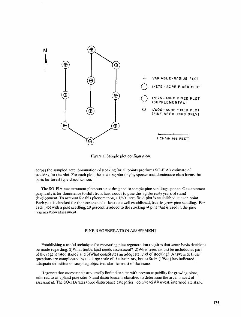
VARIABLE-RADIUS PLOT

1/275 - A C R E FIXED PLOT

1/275-ACRE FIXED PLOT(SUPPLEMENTAL)

l /600-ACRE FIXED PLOT(PINE SEEDLINGS ONLY)

1 CHAIN (66 FEET)

Figure 1. Sample plot configuration.

across the sampled acre. Summation of stocking for all points produces SO-FIA's estimate ofstocking for the plot. For each plot, the stocking plurality by species and dominance class forms thebasis for forest type classification.

The SO-FIA measurement plots were not designed to sample pine seedlings, per se. One commonperplexity is for dominance to shift from hardwoods to pine during the early years of standdevelopment. To account for this phenomenon, a 1/600 acre fixed plot is established at each point.Each plot is checked for the presence of at least one well established, free-to-grow pine seedling. Foreach plot with a pine seedling, 10 percent is added to the stocking of pine that is used in the pineregeneration assessment.

PINE REGENERATION ASSESSMENT

Establishing a useful technique for measuring pine regeneration requires that some basic decisionsbe made regarding: l)What timberland needs assessment? 2)What trees should be included as partof the regenerated stand? and 3)What constitutes an adequate level of stocking? Answers to thesequestions are complicated by the large scale of the inventory, but as Stein (1984a) has indicated,adequate definition of sampling objectives clarifies most of the issues.

Regeneration assessments are usually limited to sites with proven capability for growing pines,referred to as upland pine sites. Stand disturbance is classified to determine the area in need ofassessment. The SO-FIA uses three disturbance categories: commercial harvest, intermediate stand

135

management, and natural disturbance. Classification of commercial harvest is based on cuttingintensity and inspection of the residual stand:

Clearcut - removal of all growing stock and/or rough and rotten trees.

Partial cut - pine selection cuts, diameter limit cuts, highgrading, or any other practice that tends toremove the most marketable trees, leaving a residual stand of growing stock and/or rough and rottentrees.

Other harvest - seed tree cuts, shelterwood cuts, and salvage cuts.

Pine regeneration assessment focuses on clearcut and partial cut timberland. Other harvests can beexamined after residual trees are felled. Timberland that was cleared for nonforestry use is excluded.

The SO-FIA includes trees of all size classes in the regeneration assessment based on managementpractices of the region, the "snapshot" nature of the sample, and the need for consistency with otherSO-FIA estimates. The most prevalent harvest practice in the South Central region is partial cutting,primarily due to its use by nonindustrial private owners who rely heavily on natural regeneration(McWilliams 1989). Thus, pole and sawtimber size trees need to be included for consistency withSO-FIA's concept of area occupancy, which underlies all stocking related variables.

Residual pine stocking is evaluated for the growing stock component of the post harvest stand,whether the trees originated from planting, seeding, or were left from the previous stand. Thisdeviates slightly from forest type and stand size variables that are based on all live trees. The growingstock limitation ensures that only trees with management potential are included. The differencebetween using all live and growing stock trees is minor in terms of the results.

Limiting the regeneration assessment to nonsuppressed trees helps to improve the ability to predictfuture species composition. As indicated in the previous section, SO-FIA's stocking calculation isoriented towards dominant trees of the existing canopy. Overtopped trees can be screened out of thestocking summation.

DATA ANALYSIS

Pine stocking is grouped into classes to provide a relative measure of success:

Low - less than 30 percent stocked with pine.

Medium - from 30 to 59 percent stocked with pine.

High - at least 60 percent stocked with pine.

Pine stocking classes furnish the analyst with an indication of future species composition. A standwith a high stocking of pine will usually develop into a pure pine stand. Some medium stocked standswill develop into pure pine stands, while others will contain a mixture of pine and hardwoods. In theabsence of later hardwood control, stands with a low stocking of pine usually evolve into hardwoodstands. Pine stocking classes provide more information than the existing forest type classificationsbecause of shifts in species plurality that often occur soon after harvest.

For analytical purposes, pine stocking classes are used in conjunction with other plot leveldescriptors. Regeneration success, on a regional scale, is related to ownership and preharvest forest

136

Table l.-Area of harvested pine-site timberland retained as forest byownership, forest type, and pine stocking class.

Ownershipand

forest typePastarea

Pine stocking class

Total Low Medium High

IndustrialPineMixedHardwood

Total

NonindustrialPineMixedHardwood

Total

All privatePineMixedHardwood

Total

9.44.433

4.42.01.4

-Million acres-

0.70.50.6

1.00.60.3

2.70.90.5

17.1 7.8 1.8 1.9 4.1

14.910.012.4

4.92.92.7

1.41.30.9

1.21.00.5

2.30.60.3

37.3

24.314.415.7

10.5 4.6

9.3 2.04.9 1.84.1 2.5

2.7

2.21.60.8

3.2

5.01.50.8

54.4 18.3 6.4 4.6 7.3

Source: The most recent forest inventories of Alabama (1982), Arkansas (1988),Louisiana (1984), Mississippi (1987), Oklahoma (1986), and Texas (1986).Industrial timberland includes land under long-term lease from nonindustrialprivate owners.

. type. In general, pine regeneration is more successful on industrial timberland and following harvestof pine forest types.

To illustrate, table 1 shows the distribution of harvested timberland by ownership, preharvest foresttype, and pine stocking class based on a study conducted in six states (McWilliams 1989). The resultsindicate that 61 percent of the harvested pine type timberland owned by forest industry had a highstocking of pine. The estimate of success increases to 84 percent if stands with medium stocking areincluded. Adding the classes together may be justified because of the intensity of harvesting onindustrial timberland. Nearly half of the pine type timberland was harvested (compared to roughlyone-third of the nonindustrial pine forest).

For nonindustrial private owners, success estimates for harvested stands ranged from 47 percent forhigh stocking to 71 percent for high and medium stocking combined. Including medium stockedstands may also be logical for nonindustrial owners because they often have limited investmentcapital, and mixed stand management offers a viable low cost alternative (Cain 1988, Phillips andAbercrombie 1987). Although a relative measure of success is often preferred, some applicationsrequire a single statement regarding regeneration success. In such a case, it is useful to refer to theoverall replacement rate for harvested pine stands. The replacement rate is computed by dividing the

137

area with a high stocking of pine by the area of pine stands that was harvested. In the example, therate is 93 percent for forest industry and 65 percent for nonindustrial owners.

Percentages must be used with caution for trend analysis. For example, a static replacement ratebetween two inventories could imply no change in the total area regenerated. This is not the case ifthe area harvested increased during the inventory period.

The SO-FIA's systematic sampling design provides a spatial dimension to the analyses. Figure 2depicts a sequence of maps showing the regeneration situation for nonindustrial owners inMississippi. Screening the sample of pine site plots for harvesting, residual pine stocking, and siteproductivity highlights the regional dimension. If the most productive sites are a priority, the southernhalf of the State has the largest area in need of pine regeneration.

DISCUSSION

Successive forest inventories reflect the period prior to measurement (inventory periods are usually 7to 10 years). As such, regeneration surveys measure the effects of economic cycles, harvest intensity,weather, disease, and other factors. This is an important advantage in contrast to the limitationsassociated with using planting records to gauge regeneration following harvest. Planting records donot reflect plantation failure and exclude natural regeneration. Drought and fusiform rust infectionhave been significant factors in recent years (Burnett 1987, Lenhart et al. 1988). An informal study inTexas predicted a 60 percent loss of seedlings planted in 1988 due to the severe summer drought(Cohen 1988). Also, planting records include significant areas planted on marginal cropland as partof the Conservation Reserve Program. Such plantings do not contribute to regeneration of harvestedstands.

Users of regeneration survey results need to be cognizant of the implications of estimationprocedures. Applying a single stocking standard to a range of management intensities and siteconditions imposes some limits. Another limitation involves the lag time between harvest andregeneration. All of the current inventory results indicate increased harvesting that may haveoccurred in the latter years of the inventory periods. Because of this, it is possible that some of theharvested timberland was sampled between harvest and the development of regeneration.Regeneration assessment must be ongoing if the dynamism of southern forestry is to be described andmajor trends are to be identified.

138

Figure 2. Spatial analysis of pine regeneration on nonindustrial private pine site timberland inMississippi, 1978-87: a)All plots, b)Harvested plots, c)Harvested plots with medium or low pinestocking, and d)Harvested plots with medium or low pine stocking on high sites (capable of growingat least 120 cubic feet per acre annually).

139

REFERENCES

Burnett, H. 1987: The great drought of 1986. American Forests. May/June issue, pp. 22-25.

Cain, M.D. 1988: A low-cost technique for increasing pine volume production in mixedpine-hardwood stands. Research Paper SO-246. New Orleans,LA: U.S. Department of

Agriculture, Forest Service, Southern Forest Experiment Station. 9 p.

Cohen, M. 1988: Drought measure spells relief for stricken forest farmers. Forest Farmer,Vol. 48, No. 1, pp. 24-25.

Kaltenberg, M.C. 1984: Evaluation of regeneration sampling methods: a monte carlo analysisusing simulated stands. In: New Forests for a Changing World: Proceedings of the 1983Convention of the Society of American Foresters; 1983 October 16-20, Portland, OR: 27-34.

Lenhart, J. D., W.T. McGrath, and T.L. Hackett. 1988: Fusiform rust trends in EastTexas: 1969-1987. Southern Journal of Applied Forestry, Vol. 2, No. 4, pp. 259-261.

McWilliams, W.H. 1989: Harvest activity and residual pine stocking on private lands of sixSouth Central Coastal States. Southern Journal of Applied Forestry, (in press).

Phillips, D.R. and J.A. Abercrombie, Jr. 1987: Pine-hardwood mixtures - a new conceptin regeneration on harvested lands. Southern Journal of Applied Forestry, Vol. 11, No. 4,pp. 192-197.

Stein, W.I. 1984a: Reforestation surveys: an overview. In: New Forests for a ChangingWorld: Proceedings of the 1983 Convention of the Society of American Foresters; 1983October 16-20, Portland, OR: 2-6.

Stein, W.I. 1984b: Fixed-plot methods for evaluating forest regeneration. In: New Forestsfor a Changing World: Proceedings of the 1983 Convention of the Society of AmericanForesters; 1983 October 16-20, Portland, OR: 20-26.

USDA, Forest Service. 1988: The South's fourth forest: alternatives for the future. FRR-24.National Technical Information Service, Springfield, VA. 512 p.

140