monitoring product size and edging from bivariate proﬁle data

mss # 1674.tex; art. # 02; 46(3)

Monitoring Product Size and

Edging from Bivariate Profile Data

ROMAN VIVEROS-AGUILERA

McMaster University, Hamilton, Ontario L8S 4K1, Canada

STEFAN H. STEINER and R. JOCK MACKAY

University of Waterloo, Waterloo, Ontario N2L 3G1, Canada

Profile data consist of the coordinates of points along the edge of the product. Often, several hundredpoints are involved. Mechanical and automated procedures (e.g., scanning) are used in data gathering.The large data dimensionality presents challenges in the development of control charts to monitor productprofiles. The data also show strong cross-correlations between points close to one another. In this article,using the leading principal components of the coordinate covariance matrix, we develop Hotelling’s T 2

and upper exponentially weighted moving average (EWMA) charts to monitor product size. The methodsare extended to monitor product edging using the angles between the normal vectors of the blueprintand sample profiles. We use a Markov chain approximation to calculate average run length. Throughsimulations, we assess the performance of the proposed methods and show the upper EWMA chart exhibitgood performance in most of the o↵-target scenarios considered. A comparison with existing methodsreveals that the proposed charts are very competitive and require fewer distributional assumptions.

Key Words: Angular Vectors; Average Run Length; EWMA Chart; Hotelling’s T 2 Chart; Principal Com-ponents; Smoothing; SPC.

1. Introduction

BLUEPRINTS or designs of mechanical parts aredrawn to represent graphically detailed part

specifications. Computer-aided design (CAD) pack-ages are usually used in this process. Often the partsdisplay flat forms, for instance, when obtained bycutting from metal sheets and other flat materials.A turning process using a lathe is another example.If the flat material exhibits su�ciently homogeneousthickness, the main features of the workpiece are de-

Dr. Viveros-Aguilera is Professor in the Department of

Mathematics and Statistics. He is a Member of ASQ. His email

address is [email protected].

Dr. Steiner is Professor in the Department of Statistics and

Actuarial Science. He is a Fellow of ASQ. His email address is

[email protected].

Dr. MacKay is Adjunct Professor in the Department of

Statistics and Actuarial Science. His email address is jock

[email protected].

termined by its edge. In what follows, we refer tothe planar representation of the edge as the shape orprofile of the workpiece.

Shape specifications include dimensional charac-teristics such as length and width; curvature such asstraightness, circularity, and ovality; and edge tex-ture such as roughness and waviness. No matter howtightly a process is run, manufacturers recognize thatno two workpieces made from the same design areidentical. Every process is bound to exhibit some in-herent variation in shape from part to part. The roleof statistical process control methods is to spot whenthe variation in the profile of the manufactured partsshows deviation beyond the natural process varia-tion.

The concepts and methods discussed in this articleapply equally to shapes from cross-sections of three-dimensional parts, e.g., the profile of a workpiece ata given height of the part when it rests on a levelsurface.

Vol. 46, No. 3, July 2014 199 www.asq.org

mss # 1674.tex; art. # 02; 46(3)

200 ROMAN VIVEROS-AGUILERA, STEFAN H. STEINER, AND R. JOCK MACKAY

Profile monitoring initially focused on situationswhere the profiles are adequately described by a lin-ear regression between a single product quality vari-able and a single predictor. The primary objective isto uncover when the linear association breaks downin the Phase II process operation (see, e.g. Mah-moud and Woodall (2004) and Sullivan (2002) formore details on Phase I and Phase II analyses).The methods make use of the residuals or coe�-cient estimates (e.g., Kim et al. (2003), Mahmoudand Woodall (2004), Gupta et al. (2006), among oth-ers) or are based on change-point analysis (e.g., Zouet al. (2006)). The methods were then extended toprocesses where multiple linear or polynomial re-lationships between a single quality indicator andpredictors are appropriate (e.g., Zou et al. (2007),Kazemzadeh et al. (2008), Noorossana et al. (2010)).In the more recent research, attention centers oncurved or nonlinear profiles using parametric nonlin-ear regression (e.g., Williams et al. (2007a, 2007b))and nonparametric charts (Qiu et al. (2010)).

In the above references, the profile description isunivariate. For instance, Qiu et al. (2010) considerdata for m profiles, where the ith profile consists ofni observations, {xij , yij}, 1 j ni, 1 i m,described by yij = g(xij) + fi(xij) + ✏ij where g(x)is the target profile, fi(x) models the variation ofthe ith profile around the target, and ✏ij is a ran-dom error, the source of which is typically measure-ment error. Here x is a predictor or covariate, suchas time or distance, depending on the process. Thisis a mixed-e↵ects model and Qiu et al. (2010) fit itnonparametrically to Phase I data.

Colosimo et al. (2008) discuss bivariate profileswhere the data are many pairs of (x, y) values corre-sponding to points along the edge of a product. Un-like the previously discussed profiles, the planar rep-resentation of the bivariate profiles are closed-loopcurves. Naturally, measurement error can occur inboth x and y coordinates. Colosimo et al. (2008) bor-row ideas from spatial statistics, specifically spatialcorrelation, to develop a parametric normal regres-sion model to describe the profiles. After fitting themodel to a sample of Phase I profiles, they use the es-timated model coe�cients to construct a Hotelling’sT 2 chart to monitor part size from Phase II sam-ple profiles. Additionally, they provide an informa-tive discussion on many issues in product manufac-turing from an engineering perspective that conveyswell the context for profile control charts in industrialapplications.

We focus on bivariate profiles and develop alter-native charts to those of Colosimo et al. (2008) tomonitor the size of parts. The methods proposed arenonparametric and straightforward to implement us-ing conventional statistical software such as R, SAS,or MATLAB. We then extend the methods to moni-tor edge smoothness from the same bivariate profiledata.

In the next section, we describe formally the bi-variate profiles of interest along with practical as-pects of profile data gathering. A short review followson principal component analysis upon which the con-struction of the proposed Hotelling’s T 2 and expo-nentially weighted moving average (EWMA) chartsfor monitoring product size and edging are built.Details on the charts, including average run length(ARL) calculation, are provided. We then focus onsimulation of sample profile data yielding rough andsmooth sample profiles useful in chart calibration andperformance assessment. Next, the results of a nu-merical study of chart performance is presented usingsix o↵-target scenarios. A study that compares nu-merically the proposed methods with the main com-peting charts follows. The paper ends with a discus-sion of the advantages and limitations of the pro-posed methods.

2. Bivariate Profiles:Target, Sample and Data Gathering

Bivariate profile data consist of the (x, y) coordi-nates of points sequentially located along the edgeof a manufactured item. If n points are sampled, theprofile data take the form p = {(xj , yj)} n

j=1. Ide-ally, the points should be uniformly spread along theedge for slowly changing sections of the product andtighter on fast changing sections. Naturally, keepingtrack of order is critical.

The target profiles considered here are planarclosed loops and thus can adequately be describedby bivariate functions indexed over an interval as

p0(s) = (x0(s), y0(s)), s 2 [a, b]; p0(a) = p0(b).(1)

The components will be continuous and di↵erentiableexcept for a finite number of points representing “cor-ners” in the items profiled. Representation (1) al-lows for curved loops of arbitrary shapes. Througha simple linear transformation, one could work with[a, b] = [0, 1].

Most authors working on profile monitoring fo-cus on representations of the regression type. For in-

Journal of Quality Technology Vol. 46, No. 3, July 2014

mss # 1674.tex; art. # 02; 46(3)

MONITORING PRODUCT SIZE AND EDGING FROM BIVARIATE PROFILE DATA 201

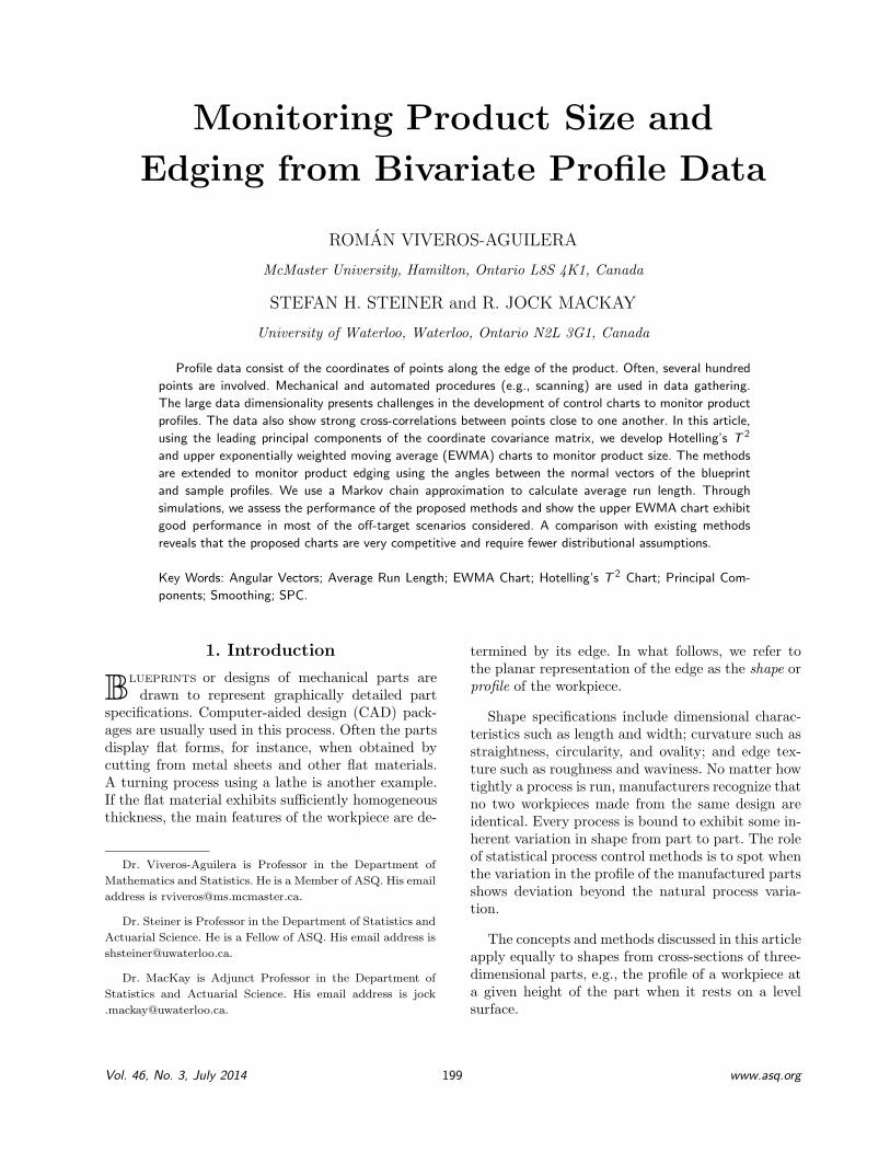
FIGURE 1. Circle and Oval Target Profiles, and Sample Profile Data With and Without Measurement Error.

stance, Qiu et al. (2010) work with

(x, g(x)), x 2 [a, b], (2)

where x is treated as a covariate. Note that equation(2) can be represented as equation (1) by defining

(x0(s), y0(s)) = (s, g(s)), s 2 [a, b]. (3)

Profiles described by equation (2) are essentially or-dinary univariate functions. Generally they are in-adequate to describe profiles shaped as closed loops,as they can represent only sections of such profiles.However, as discussed in the next section, dependingon how the data are gathered, there are instanceswhere closed loops can be unfolded, enabling a uni-variate treatment.

Several target and sample profiles are displayed inFigure 1. In Figures 1(a) and 1(c), the target profileis a circle with functional representation

p0(s) = (x0(s), y0(s))= (r cos(s), r sin(s)), 0 s 2⇡, (4)

where r is the radius of the circle. In Figure 1(b), thetarget profile is a pointed oval with functional form

p0(s) = (x0(s), y0(s))

=

8<:

(1.5 sin(2⇡s), 8s), 0 s 0.5;(1.5 sin(2⇡(s� 0.5)),8(1� s)), 0.5 s 1.

(5)

Sample profiles of 150 points each are displayedin Figure 1. In Figure 1(a) and 1(b), the pointsare joined by segments to identify the sequence.These cases correspond to situations where substan-tial measurement error is present. A smooth sampleprofile is shown in Figure 1(c). Profile data of this

type are typically obtained when a high-precision in-strument, such as a laser scanner, is used in the data-gathering process.

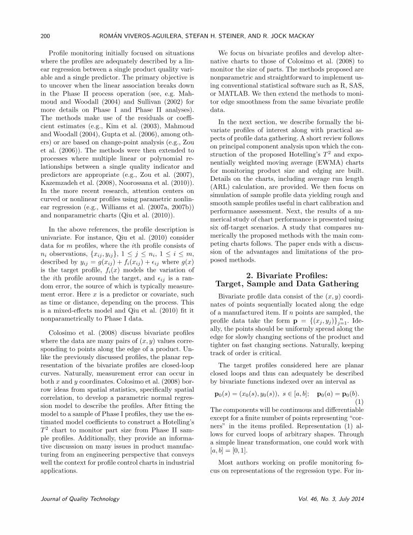
For planar profiles exhibiting a convex shape (i.e.,↵(x1, y1)+(1�↵)(x2, y2) lies inside the profile for ev-ery pair of points (x1, y1) and (x2, y2) on the profileand every 0 ↵ 1), one may collect the data by themethod of angular spanning. First, identify a “cen-ter” point for the part. In principle, any point withinthe profile can be used as center, provided the point isconsistently used for all the parts. Second, for a givenangle s in radians (0 s 2⇡), trace the segment atangle s starting from the center and extending up tothe edge. Last, identify the coordinates (x(s), y(s)) ofthe point of intersection. The process is illustrated inFigure 2(a). One then repeats the process for selectedangles s1, s2, . . . , sn. Here [a, b] = [0, 2⇡]. The result-ing sample data take the form {(x(sj), y(sj))}n

j=1.Colosimo et al. (2008) follow this approach using theradial distances in their analysis.

In other applications, a mechanical tool and objectrotation are used to gather data on the shape of ob-jects. The mechanical device has a flexible arm that iscapable of retracting or extending as it comes in con-tact with objects. The method is depicted in Figure2(b). First, fix the device at some point P . Second,center and fix the product at another point C, whereP and C are far enough apart to allow the arm toreach the edge of the object for which we wish tocapture the profile. Third, rotate the object aroundC and record the distance r from the device to theedge of the object. The process may be performed ei-ther continuously, for instance on graph paper, or atdi↵erent points in time s1, s2, . . . , sn as the object ro-tates at a constant speed. The data can be convertedto coordinates {(x(sj), y(sj))}n

j=1. Alternatively, one

Vol. 46, No. 3, July 2014 www.asq.org

mss # 1674.tex; art. # 02; 46(3)


FIGURE 2. Gathering Sample Profile Data by (a) Angular Spanning and (b) Retractable-Armed Device and Object Rotation.

can work with the radial distances from the center Cto the edge of the part.

Greater data-gathering e�ciency and precisionare achieved through the use of a laser scanner tocapture the shape of an item. Companies use profilelaser scanners routinely in several stages of a manu-facturing process, including part inspection, roboticguidance, and shape check. In addition, scanners typ-ically record a larger number of points on the prod-uct’s edge than do manual and other low-tech meth-ods, thus providing a more detailed description ofthe shape. Another advantage is their capability ofcapturing nonconvex shapes, a challenge for manualand mechanical methods.

3. Principal ComponentsChart for Product Size

3.1 Principal Components of Phase I SampleProfiles

Following the familiar approach for control-chartconstruction, the starting point is the availabilityof process data amenable to estimation of the pro-cess parameters required in setting up and calibrat-ing the chart. After careful inspection and possiblysome data cleaning, we assume that sample profiledata from m parts are available when the process isstable. Further, assume that the data were collectedsystematically so that the indexing of points is thesame across the m parts. We refer to this dataset asthe Phase I or training sample profiles.

Represent the Phase I profiles as

pi = {(xij , yij) = (xi(sj), yi(sj))}nj=1,

i = 1, 2, . . . ,m.

Each profile will be treated as a row vector with 2ncomponents, namely

pi = (xi1, xi2, . . . , xin, yi1, yi2, . . . , yin),i = 1, 2, . . . ,m.

The average Phase I profile is

p0 = (x01, x02, . . . , x0n, y01, y02, . . . , y0n)

=mX

i=1

pi/m. (6)

We further assume that measurement error is ei-ther small or has been reduced, for instance, by datasmoothing. Thus, the sample profiles should typicallylook like that in Figure 1(c). Section 4 on profile sim-ulation provides further details.

An estimate of the covariance matrix of the pro-file coordinates is a key ingredient of the proposedmultivariate control chart discussed in the next sec-tion. We use the m training profiles to produce thisestimate. The main consideration here is that thecoordinates of points physically close in the profileof an item likely exhibit high (positive) correlationwhile points far apart will not. We denote by S0

the within-profile covariance matrix associated witha profile vector p for items produced under normalprocess operation.


mss # 1674.tex; art. # 02; 46(3)


We will work with the sample covariance matrixestimate, namely,

S0 =

Sxx Sxy

S0xy Syy

!,

with the n ⇥ n matrices Sxx, Sxy, and Syy beingthe estimates of the within x, between x and y andwithin y covariance matrices, respectively.

Note that, should there be an underlying structure(e.g., time series or other) in the x and y componentsfor the edge points of the profile, it will be reflectedin the above estimates. An attractive feature of theproposed approach is that such a structure does notneed to be made explicit. However, if one wishes toinvestigate the nature and extent of such serial cor-relations and is able to identify a viable time-seriesmodel for the Phase I profile data, the above covari-ance estimates can be replaced with the correspond-ing estimates from the time-series model.

Our proposed monitoring approach focuses on theleading principal components that explain the ma-jority of the variability in the Phase I profile data.The main motivation is a reduction in dimension inthe monitoring problem by concentrating on the di-rections that drive the variability in the profile data.

The analysis will be based on the well-known spec-tral decomposition for quadratic forms (see, e.g.,Johnson and Wichern (2007), p. 61; Krzanowski(2008), p. 126). Specifically, if �1,�2, . . . ,�2n are theeigenvalues of S0 (we assume that �1 � �2 � · · · ��2n) and e1, e2, . . . , e2n the associated normalizedcolumn eigenvectors, then

S0 = U⇤U0, (8)

where U is the 2n ⇥ 2n matrix with corre-sponding columns given by the eigenvectors U =(e1|e2| · · · |e2n), and ⇤ is the 2n⇥2n diagonal matrixof the eigenvalues. Because the normalized eigenvec-tors are also orthogonal, then e0iei = 1 and e0iej = 0for i 6= j, leading to U0U = UU0 = I2n where I2n isthe 2n⇥ 2n identity matrix and

U0S0U = ⇤.

Because S0 is a (sample) covariance matrix, it is pos-itive semidefinite. As a result, all of its eigenvaluesare nonnegative. We chose U so that the eigenvaluesare ordered from largest to smallest.

The principal components for an n-point profilep = (x1, x2, . . . , xn, y1, y2, . . . , yn) are

c = U0p0,

with estimated covariance matrix

Var(c) = U0S0U = ⇤.

A measure of overall variability in a multivariatedata set is the total sample variability (tsv), definedas the sum of all the sample variances for the indi-vidual variables,

tsv = tr(S0), (9)

where tr(A) denotes the trace of matrix A. Becausetr(AB) = tr(BA), it follows from equations (8) and(9) that

tsv = tr(⇤) =2nXi=1

�i.

Thus, the percentage of the total variability ac-counted for by the first k eigenvalues is

Pk = 100⇥Pk

i=1 �iP2ni=1 �i

%, k = 1, 2, . . . , 2n. (10)

Consider the first k principal components, namely

ck = U0kp

0, (11)

where Uk = (e1|e2| . . . |ek). One can readily showthat

V ar(ck) = U0kS0Uk = ⇤k, (12)

where ⇤k = diag(�1,�2, . . . ,�k). Thus, the totalvariability in the first k principal components isPk

i=1 �i and, hence, the percentage of the total vari-ability in the full data explained by the first k prin-cipal components is Pk as given by equation (10).

3.2 Hotelling’s T 2 and Upper EWMA Chartsfor Product Size

Direct application of standard multivariate con-trol charts requires inverting the 2n⇥ 2n sample co-variance matrix S0. With large n and strong cross-correlations, S0 is nearly singular. To get aroundthis di�culty, we propose to build charts using thescores from the leading principal components. Themain motivations of the proposed approach are asfollows. In many high-dimensional data sets, a smallto moderate number of leading principal componentsoften explain the majority of the variability in thedata, thus providing a substantial reduction in di-mension. In addition, the principal components as-sociated with the larger eigenvalues tend to be mostsensitive to changes in the patterns of multivariatedata. Note also that the principal components arenonparametric in the sense that no statistical model


mss # 1674.tex; art. # 02; 46(3)


for the multivariate data is needed for their calcula-tion and interpretation. There are many applicationsof principal components in quality control, particu-larly on the use of one to three leading componentsin problems involving a large number of process vari-ables (see, e.g., Jackson (2003), chs. 6 and 7; Mont-gomery (2008), ch. 11; and the references therein).

A word of caution is necessary here. Looking atthe leading principal components helps capture thelargest sources of variation in the Phase I profile data.However, these may not always be the best for de-tecting subtle changes in the process. In other words,there is no reason why some special causes may notact in other directions. Note that this is a lurkingfeature of any data-reduction–based control chart.

From equations (11) and (12), the Hotelling’s T 2

statistic from the leading kP components for a given1⇥ 2n profile vector p is

T 2 = (p� p0)UkP ⇤�1kP

U0kP

(p� p0)0, (13)

where p0 is the Phase I sample average (6). Thequantity T 2 is a statistical distance between the sam-ple profile p and the average Phase I profile p0.

For Phase II profiles, we propose the Hotelling’sT 2 chart arising from equation (13). Specifically, oneplots T 2

t vs. t, where T 2t is the value from equation

(13) obtained for the sample profile p of an itemselected from production at sampling period t. Af-ter setting an in-control average run length ARL0,the (upper) control limit H for the T 2 chart can beobtained as the (ARL0 � 1)/ARL0 percentile of thedistribution of T 2 when the process is stable. Thepercentile can be estimated using the m T 2-valuesfrom the Phase I profiles. A better approach is to fitan appropriate statistical distribution to those valuesand then use the percentile of the fitted distributionto obtain the control limits. Note that, if the Phase IIprofiles p are stable and have an approximate multi-variate N2n(p0,S0) distribution, then T 2 follows anapproximate �2 distribution with kP degrees of free-dom. Experimentally, we found that, in many situa-tions, a gamma distribution, which contains the �2

distribution as a particular case, provides a satisfac-tory approximation to the distribution of T 2 in PhaseI. In this case, the required control limit H satisfies

P (Z H) =ARL0 � 1

ARL0(14)

where Z ⇠ Gamma(↵0,�0) and ↵0 and �0 are theshape and scale parameters of the approximatinggamma distribution.

It should be pointed out that, as with ev-ery control chart that relies on Phase I sampledata to estimate the stable process parameters, theabove method provides only approximate averagerun lengths. This stems from the fact that the pro-cess parameters are not set to their true values butto estimates. If the Phase I sample is large, the en-suing estimates have small sampling errors, leadingto more accurate ARLs.

It is well known that a more e↵ective chartto detect small persistent changes is the exponen-tially weighted moving average (EWMA) chart (e.g.,Montgomery (2008), ch. 9). Introduced by Roberts(1959), the chart has received much attention, par-ticularly for normally distributed measurements. See,for example, Crowder (1987, 1989) and Lucas andSaccucci (1990). In our situation, the quantity ofinterest T 2 follows a gamma distribution approxi-mately when the process is in-control.

If T 2t is the Hotelling’s T 2 value of equation (13)

from the Phase II sample profile pt at sampling pe-riod t, the standard EWMA chart statistic is

Wt = (1� �)Wt�1 + �T 2t , (15)

where 0 < � 1 is the smoothing parameter withthe starting value W0 set at the expected value forT 2. Assuming T 2 follows a Gamma distribution withshape ↵0 and scale �0 when the process is stable,then we let W0 = ↵0�0.

Because the aim is primarily to catch process dete-rioration, only large values of Wt are of interest. Someauthors advocate the use of a reflecting barrier in theEWMA and other charts, aimed at injecting highere�ciency in detecting excursions from the stable con-dition (see, e.g., Gan (1992, 1994), Zhang and Chen(2004), Knoth (2005), Li et al. (2009)). The idea isto prevent the statistic from reaching values too lowthat unduly slow its reaction to process changes. Themodified resulting chart, termed the upper EWMA,is based on the statistic

Zt = max{B, (1� �)Zt�1 + �T 2t }, (16)

where B (0 B < 1) is the barrier. Setting B = 0leads to equation (15). A tested and recommendedchoice for B is E(T 2) for T 2, calculated from on-target profiles. Thus, if T 2 follows a Gamma(↵0,�0)distribution under stable conditions, then B = ↵0�0.Further, the initial chart value Z0 can be taken to beZ0 = E(max{B,T 2}), again, calculated for T 2 fromthe appropriate gamma distribution. One can show


mss # 1674.tex; art. # 02; 46(3)


that, when T 2 follows a Gamma(↵0,�0) distribution,

Z0 = BG(B;↵0,�0) + ↵0�0[1�G(B;↵0 + 1,�0)],(17)

where G(x;↵0,�0) denotes the gamma distributionfunction. We use the upper EWMA chart throughoutour analysis with the above choices for B and Z0.

Calibrating the upper EWMA chart involves de-termining the control limit H that yields a speci-fied in-control average run length ARL0 with thechart signaling when Wt > H for the first time. TheMarkov chain method works well here. The methodis described in detail for the standard EWMAby Lucas and Saccucci (1990) for a normally dis-tributed chart statistic. In our situation, T 2 followsa Gamma(↵0,�0) distribution. The relevant result isthat, given any control limit H, the in-control aver-age run length ARL0 is approximated by

ARL0 = v00(I�P0)�11, (18)

where P0 is the N ⇥ N transition probability ma-trix with entries given in equation (19) and v0 is theN ⇥ 1 vector of 0s except for the entry correspond-ing to the state containing Z0 from equation (17),where 1 is entered instead. The larger the value of N ,the better the approximation. Then H is varied untilARL0 reaches a desired (large) value. The form of the

transition probability matrix P0 = (p(i, j)) N Ni=1 j=1 is

p(i, j) =

8>>>>>><>>>>>>:

G⇣

Cj�(1��)Ci

� + L� ;↵0,�0

⌘, j = 1;

G⇣

Cj�(1��)Ci

� + L� ;↵0,�0

⌘�G

⇣Cj�(1��)Ci

� � L� ;↵0,�0

⌘,

2 j N ;(19)

for 1 i N , where L = (UCL � B)/(2m),Ck = B + (2k � 1)L, and G(x;↵0,�0) is the gammadistribution function.

Table 1 contains the control limit H when ARL0 =400 for an in-control gamma distributed T 2 for se-lected values of the shape parameter ↵0 with scalefixed at �0 = 1. In all cases, � = 0.1. If �0 6= 1, therespective control limit is �0H, where H is the con-trol limit from Table 1 for the same ↵0. Interpolationcan be used for shape values between those in the ta-ble. For the H values in Table 1, a total of N = 1000states were used, resulting in a 1000⇥1000 transitionprobability matrix.

4. Simulating Profile Data

Many defects in manufactured parts appear in theform of cracks, scratches, or insu�cient/excess ma-

TABLE 1. Control Limit (H) for the Upper EWMA Chart for In-Control Average Run Length ARL0 = 400 andGamma Distributed Phase I T 2 for Several Shape Parameter Values ↵0 and Scale �0 = 1 (� = 0.1 in All Cases)

↵0 0.1 0.3 0.5 0.7 1.0 2.0 3.0H 0.4008 0.7652 1.0699 1.3528 1.7560 3.0141 4.2110

↵0 4.0 5.0 6.0 7.0 8.0 9.0 10.0H 5.3765 6.5223 7.6539 8.7750 9.8877 10.9934 12.0935

↵0 11.0 12.0 13.0 14.0 15.0 16.0 17.0H 13.1886 14.2796 15.3667 16.4506 17.5315 18.6099 19.6858

↵0 18.0 19.0 20.0 22.0 24.0 26.0 28.0H 20.7594 21.8311 22.9009 25.0354 27.1639 29.2871 31.4058

↵0 30.0 32.0 34.0 36.0 38.0 40.0 42.0H 33.5203 35.6309 37.7382 39.8424 41.9438 44.0424 46.1387

↵0 44.0 46.0 48.0 50.0 55.0 60.0 65.0H 48.2328 50.3245 52.4145 54.5025 59.7151 64.9184 70.1134

↵0 70.0 75.0 80.0 85.0 90.0 95.0 100.0H 75.3007 80.4817 85.6569 90.8264 95.9912 101.1513 106.3072


mss # 1674.tex; art. # 02; 46(3)


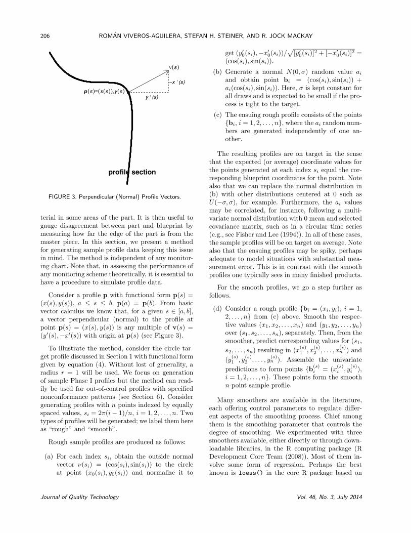
FIGURE 3. Perpendicular (Normal) Profile Vectors.

terial in some areas of the part. It is then useful togauge disagreement between part and blueprint bymeasuring how far the edge of the part is from themaster piece. In this section, we present a methodfor generating sample profile data keeping this issuein mind. The method is independent of any monitor-ing chart. Note that, in assessing the performance ofany monitoring scheme theoretically, it is essential tohave a procedure to simulate profile data.

Consider a profile p with functional form p(s) =(x(s), y(s)), a s b, p(a) = p(b). From basicvector calculus we know that, for a given s 2 [a, b],a vector perpendicular (normal) to the profile atpoint p(s) = (x(s), y(s)) is any multiple of v(s) =(y0(s),�x0(s)) with origin at p(s) (see Figure 3).

To illustrate the method, consider the circle tar-get profile discussed in Section 1 with functional formgiven by equation (4). Without lost of generality, aradius r = 1 will be used. We focus on generationof sample Phase I profiles but the method can read-ily be used for out-of-control profiles with specifiednonconformance patterns (see Section 6). Considergenerating profiles with n points indexed by equallyspaced values, si = 2⇡(i� 1)/n, i = 1, 2, . . . , n. Twotypes of profiles will be generated; we label them hereas “rough” and “smooth”.

Rough sample profiles are produced as follows:

(a) For each index si, obtain the outside normalvector ⌫(si) = (cos(si), sin(si)) to the circleat point (x0(si), y0(si)) and normalize it to

get (y00(si),�x00(si))/p

[y00(si)]2 + [�x00(si)]2 =(cos(si), sin(si)).

(b) Generate a normal N(0,�) random value ai

and obtain point bi = (cos(si), sin(si)) +ai(cos(si), sin(si)). Here, � is kept constant forall draws and is expected to be small if the pro-cess is tight to the target.

(c) The ensuing rough profile consists of the points{bi, i = 1, 2, . . . , n}, where the ai random num-bers are generated independently of one an-other.

The resulting profiles are on target in the sensethat the expected (or average) coordinate values forthe points generated at each index si equal the cor-responding blueprint coordinates for the point. Notealso that we can replace the normal distribution in(b) with other distributions centered at 0 such asU(��,�), for example. Furthermore, the ai valuesmay be correlated, for instance, following a multi-variate normal distribution with 0 mean and selectedcovariance matrix, such as in a circular time series(e.g., see Fisher and Lee (1994)). In all of these cases,the sample profiles will be on target on average. Notealso that the ensuing profiles may be spiky, perhapsadequate to model situations with substantial mea-surement error. This is in contrast with the smoothprofiles one typically sees in many finished products.

For the smooth profiles, we go a step further asfollows.

(d) Consider a rough profile {bi = (xi, yi), i = 1,2, . . . , n} from (c) above. Smooth the respec-tive values (x1, x2, . . . , xn) and (y1, y2, . . . , yn)over (s1, s2, . . . , sn), separately. Then, from thesmoother, predict corresponding values for (s1,s2, . . . , sn) resulting in (x(s)

1 , x(s)2 , . . . , x(s)

n ) and(y(s)

1 , y(s)2 , . . . , y(s)

n ). Assemble the univariatepredictions to form points {b(s)

i = (x(s)i , y(s)

i ),i = 1, 2, . . . , n}. These points form the smoothn-point sample profile.

Many smoothers are available in the literature,each o↵ering control parameters to regulate di↵er-ent aspects of the smoothing process. Chief amongthem is the smoothing parameter that controls thedegree of smoothing. We experimented with threesmoothers available, either directly or through down-loadable libraries, in the R computing package (RDevelopment Core Team (2008)). Most of them in-volve some form of regression. Perhaps the bestknown is loess() in the core R package based on


mss # 1674.tex; art. # 02; 46(3)


fitting local polynomial regressions. Also available inthe core R package is smooth.spline(), which fitsa cubic smoothing spline. A variant of loess() islpridge(), which fits a local polynomial regressionwith ridging, available in library lpridge of Seifert(2007). Each of these smoothing methods is nonpara-metric and produces on-target profiles whenever theoriginal rough data are on target. Also, each methodallows predictions. An interesting and important fea-ture of the smooth profiles is that neighboring pointswill tend to be similar and thus will exhibit highpositive coordinate-wise correlation while points farapart will be nearly uncorrelated.

The rough sample profile for the circle shown inFigure 1(a) contains n = 150 points generated usingthe above method, with ai values independently gen-erated from a normal distribution with mean 0 andstandard deviation 0.1. The same process producedthe rough sample profile in Figure 1(b) but using thefunctional form for the oval target profile from equa-tion (5). The smooth sample profile shown in Figure1(c) comes from a rough sample profile of n = 100points generated with independent ai ⇠ N(0, 0.1)values and smoothed using smooth.spline() withthe smoothing parameter set at spar = 0.6.

For smooth Phase I sample profiles, the role of �is to reflect the intrinsic leeway of the manufacturingprocess around the blueprint shape. Simulation oftight processes requires � to be small, while a large �recreates processes with substantial wiggling aroundthe target.

Exampe 1: Phase I Profile Sample

The purpose of this example is to illustrate theforegoing methods and to generate a sample of PhaseI profiles to be used in calibrating the proposedcharts. A sample of m = 1000 rough and smoothindependent profiles was generated employing theabove method with the circle of radius r = 1 as theblueprint. The index values were si = 2⇡(i� 1)/200radians, i = 1, 2, . . . , 200, with the ai values gener-ated from N(0,�) with � = 0.1 for the rough pro-files. The rough profiles were then smoothed usingsmooth.spline() in R with spar = 0.6 to obtain thesmooth profiles. For the remainder of the article, weconsider these sample profiles as typical of profilesseen when the process is stable. Thus, they will formthe Phase I sample.

The sample covariance matrix S0 was obtained forthe 400 coordinate values (200 x-coordinates, 200 y-coordinates) for the 1000 smooth profiles. A contour

plot for the resulting 400 ⇥ 400 sample correlationmatrix was produced and examined. The plot re-veals that x-coordinates from neighboring points arehighly positively correlated and so are the respectivey-coordinates. However, the correlations between x-and y-coordinates for neighboring points show reg-ular sections of very high positive correlations andsections of very high negative correlations as onecrosses the quadrants. This feature is explained bythe coordinate constraints arising from their circularconformance. Finally, coordinates of points far apartexhibit nearly 0 correlation.

5. Measuring and Monitoring Edging

5.1 Appraising Edging

The question addressed here is: how well does theedge of a Phase II part conform to the edge of the tar-get part? We assess this conformance relative to theconformance of the Phase I profiles when the processoperates in control.

The first task is to develop a measure of agree-ment in edging between a part and the target part.We propose to focus on the angles (in radians) be-tween the outside normal vector of the target profileand the outside normal vector at the edge of the partat points where information is available in the sampleprofile. Specifically, consider the normal vector ⌫0(s)at point p0(s) = (x0(s), y0(s)) on the target pro-file, given by ⌫0(s) = (u0(s), v0(s)) = (y00(s),�x00(s))(see Figure 3). Similarly, for a smooth sample pro-file p(s) with index values s1, s2, . . . , sn, calculatefor each s = si the outside normal vector ⌫(si) =(u(si), v(si)). To do this, one can use the coordinatederivatives provided by the univariate smoothers oruse basic numerical approximation of the coordinatederivatives, e.g., f 0(x0)

.= [f(x0+�)�f(x0��)]/(2�).Next align ⌫0(s) and ⌫(s) to have the same origin, forinstance using p(s) as origin. Finally, calculate thesigned angle (in radians) between ⌫0(s) and ⌫(s),

✓(s) = arctan✓

u0(s)v(s)� v0(s)u(s)u0(s)u(s) + v0(s)v(s)

◆. (20)

Repeat the calculation across all the available indexpoints s1, s2, . . . , sn to obtain the 1⇥n angular vector

✓ = (✓1, ✓2, . . . , ✓n) = (✓(s1), ✓(s2), . . . , ✓(sn)).

Note that the angle orientation in equation (20) iscounterclockwise, that is, ✓(s) is positive if one trav-els against the clock when going from ⌫0(s) to ⌫(s),and negative otherwise.


mss # 1674.tex; art. # 02; 46(3)


FIGURE 4. Angles Between Outside Normal Vectors forSample and Target Profiles.

Figure 4 illustrates the angles at eight points froma smooth sample profile of 200 points generated usingthe method described in Section 4 for the circle targetprofile of radius r = 1. Here, � = 0.12 and smoothingwas done using smooth.spline() with spar = 0.6.The numerical values obtained for ✓1 to ✓8 (in radi-ans) were 0.031, 0.151, 0.251, 0.168, �0.021, �0.230,0.063, and �0.053. Note that the largest disagree-ment in edging occurs at location 3, even though thetwo profiles are very close to each other. On the otherhand, at locations 1 and 5, the edging is very similar(i.e., small angles) but the target and sample profilepoints are far apart. These remarks highlight the dif-ference between product size and edging. Note thatthe angles, including signs, are invariant under posi-tive scaling, translation, and rotation.

5.2 Angular Principal Component Charts forEdging

To construct control charts for edging, one can usethe n-point Phase I smooth profiles p1,p2, . . . ,pm

discussed earlier to render Phase I angular vec-tors ✓1,✓2, . . . ,✓m by applying the method just de-scribed. We then calculate the sample covariance ma-trix A0 of the angular vectors.

Analogous to the charts developed for part size,the leading principal components of A0 can beused to construct Hotelling’s T 2 and EWMA controlcharts for edging. Denoting by Vk the n⇥ k matrixcontaining as columns the coe�cients (loadings) for

the k leading principal components of A0 with asso-ciated eigenvalues ↵1 � ↵2 � · · · � ↵k, we then usethe scores V0

k(✓�✓0)0 to calculate the Hotelling’s T 2

values

T 2 = (✓ � ✓0)Vk��1V0k(✓ � ✓0)0, (21)

where ✓ is the angular vector for a smooth sampleprofile p, ✓0 is the sample average of the Phase Iangular vectors, and � = diag(↵1,↵2, . . . ,↵k) (seeequation (13)). Thus, T 2 is a statistical distance com-paring the edging in the sample profile to the aver-age Phase I edging. The T 2 values from the m (in-control) Phase I angular vectors can be used for chartcalibration.

In Phase II, the value T 2t obtained from the angu-

lar vector ✓ = ✓t arising from a part chosen at sam-pling period t can be used to construct a Hotelling’sT 2 chart for edging by plotting T 2

t vs. t. Further, onecan use equation (15) with the angular T 2

t to obtainan upper EWMA chart for edging.

Example 2: Phase I Angular Profile Sample

Signed angular vectors were obtained by themethod just described for the smooth profiles gen-erated in example 1. Each of the m = 1000 ensuingvectors has n = 200 angles,

✓i = (✓i1, ✓i2, . . . , ✓i200)= (✓i(s1), ✓i(s2), . . . , ✓i(s200)), i = 1, 2, . . . , 1000.

We use these data as a Phase I sample of angularvectors.

The 200⇥ 200 sample covariance matrix was cal-culated for the m = 1000 Phase I angular vectors.The resulting correlation matrix resembles closelythe upper-left and lower-right sections of the corre-lation matrix for size in example 1. The salient fea-tures are a strong positive correlation between anglesfor profile points close to each other while angles forpoints far apart are nearly uncorrelated. The under-lying cause for the high correlations is the smooth-ness of the profiles.

6. Phase II Analysis

The methods proposed will be illustrated in thissection with the circle profile of equation (4) withradius r = 1 as the blueprint. On-target process op-eration generates smooth profiles as discussed in Sec-tions 4 and 5, with parameters set at r = 1, � = 0.1,and spar = 0.6. Here, r has the biggest say on the sizeof the part while � and spar determine the degree of


mss # 1674.tex; art. # 02; 46(3)


edge wiggling/smoothness. Changing these parame-ters produces varying deviations from normal stableoperation. The 1000 smooth sample profiles from ex-ample 1 and corresponding angular vectors from ex-ample 2 are used as the Phase I data.

6.1 Monitoring Size: Chart Calibration

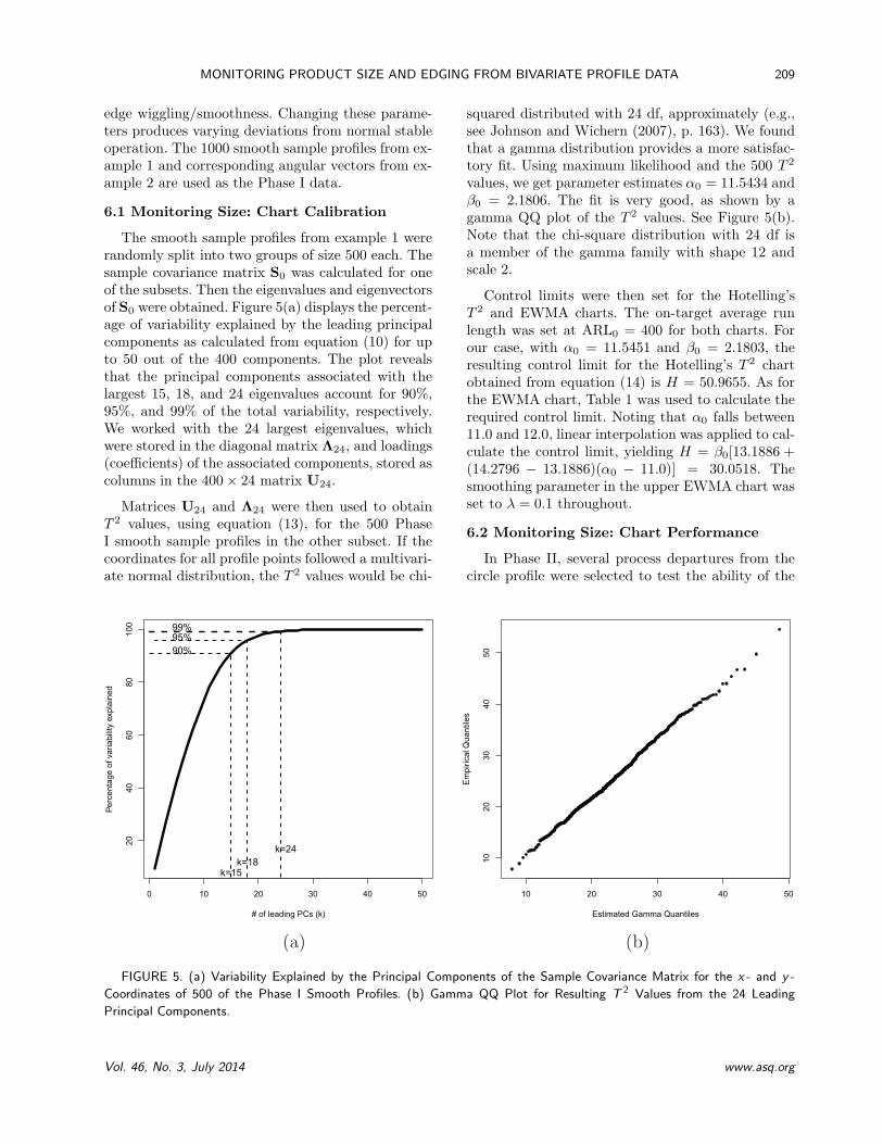
The smooth sample profiles from example 1 wererandomly split into two groups of size 500 each. Thesample covariance matrix S0 was calculated for oneof the subsets. Then the eigenvalues and eigenvectorsof S0 were obtained. Figure 5(a) displays the percent-age of variability explained by the leading principalcomponents as calculated from equation (10) for upto 50 out of the 400 components. The plot revealsthat the principal components associated with thelargest 15, 18, and 24 eigenvalues account for 90%,95%, and 99% of the total variability, respectively.We worked with the 24 largest eigenvalues, whichwere stored in the diagonal matrix ⇤24, and loadings(coe�cients) of the associated components, stored ascolumns in the 400⇥ 24 matrix U24.

Matrices U24 and ⇤24 were then used to obtainT 2 values, using equation (13), for the 500 PhaseI smooth sample profiles in the other subset. If thecoordinates for all profile points followed a multivari-ate normal distribution, the T 2 values would be chi-

squared distributed with 24 df, approximately (e.g.,see Johnson and Wichern (2007), p. 163). We foundthat a gamma distribution provides a more satisfac-tory fit. Using maximum likelihood and the 500 T 2

values, we get parameter estimates ↵0 = 11.5434 and�0 = 2.1806. The fit is very good, as shown by agamma QQ plot of the T 2 values. See Figure 5(b).Note that the chi-square distribution with 24 df isa member of the gamma family with shape 12 andscale 2.

Control limits were then set for the Hotelling’sT 2 and EWMA charts. The on-target average runlength was set at ARL0 = 400 for both charts. Forour case, with ↵0 = 11.5451 and �0 = 2.1803, theresulting control limit for the Hotelling’s T 2 chartobtained from equation (14) is H = 50.9655. As forthe EWMA chart, Table 1 was used to calculate therequired control limit. Noting that ↵0 falls between11.0 and 12.0, linear interpolation was applied to cal-culate the control limit, yielding H = �0[13.1886 +(14.2796 � 13.1886)(↵0 � 11.0)] = 30.0518. Thesmoothing parameter in the upper EWMA chart wasset to � = 0.1 throughout.

6.2 Monitoring Size: Chart Performance

In Phase II, several process departures from thecircle profile were selected to test the ability of the

FIGURE 5. (a) Variability Explained by the Principal Components of the Sample Covariance Matrix for the x - and y -Coordinates of 500 of the Phase I Smooth Profiles. (b) Gamma QQ Plot for Resulting T 2 Values from the 24 LeadingPrincipal Components.


mss # 1674.tex; art. # 02; 46(3)


charts to detect changes in size. Naturally, with high-dimensional measurements, there are many ways inwhich a profile of a manufactured product may devi-ate from its stable average. Our choices here focus onsystematic departures in size, in the degree of edgewiggling/smoothness, and on abnormalities in cer-tain spots of the product.

The following process departures were selected (inall cases spar = 0.6):

Case 1: Undersized Product. The product’s circularprofile is systematically of radius r = 0.95(rather than r = 1.0), but the degree of wig-gling/smoothness remains in control (� =0.1).

Case 2: Oversized Product. The radius is systemati-cally r = 1.03 (rather than r = 1.0) with on-target degree of wiggling/smoothness (� =0.1).

Case 3: Smoother Product. The product shows on-target radius (r = 1.0) but is systematicallysmoother than in Phase I with (� = 0.09).

Case 4: Rougher Product. The degree of wigglingis systematically higher, coming from � =0.11, but the radius is on-target (r = 1.0).

Case 5: Chipped Product. The product exhibits adent in a spot but in-control radius (r = 1.0)and degree of wiggling (� = 0.1).

Case 6: Knobby Product. A lump appears systemati-cally in the product but everything else is incontrol (r = 1.0, � = 0.1).

Illustrations of these scenarios are shown in Fig-ure 6. Note that the chip is on the southeast section(case 5) and lump in the same place (case 6). TheR code used to generate chips and lumps is availableon request.

The o↵-target average run length (ARL1) wasthen calculated for both the Hotelling’s T 2 and upperEWMA charts. Thus, ARL1 is the number of sam-ples that, on average, is needed to signal a change inthe process when a change to a particular case of thesix selected scenarios occurred. Although tedious, themost direct approach to accomplish this task is run-length simulation. However, we found that the T 2

values from o↵-target sample profiles obtained usingU24 and ⇤24 also follow closely a gamma distribu-tion but with di↵erent shape and scale parameters.Capitalizing on this finding, 2000 o↵-target smoothprofiles were generated and resulting T 2 values cal-culated. A gamma distribution was fitted and then

the average run length was calculated using the pro-posed Markov chain method with the previously cal-culated control limit H. Although the ARL1 valueswere fairly stable, the method was repeated eighttimes and the resulting ARL1 values averaged.

The two columns under “ARL1 for size” in Table2 display the results. Recall that both charts werecalibrated to ARL0 = 400. When the departure issmall (cases 4, 5, and 6), the EWMA chart performsbetter than the Hotelling’s T 2 chart. Note that, whenthe change results in smoother product (case 3), theT 2 will tend to be smaller than in the on-target caseand thus will take much longer to detect the changebecause we are using only an upper control limit (H).

6.3 Monitoring Edging: Chart Calibration

The 1000 Phase I 1⇥ 200 sample angular vectorsfrom example 2 were similarly split into two sub-sets of 500 vectors each. The 200 ⇥ 200 covariancematrix A0 was calculated for one subset and theeigenvalue/eigenvector decomposition obtained. The35 leading principal components, which explain 99%of the total variability, will be used in the charts. Theassociated eigenvalues were stored in diagonal matrix�35 and the corresponding loadings (eigenvectors) ascolumns in matrix V35.

Next, the T 2 values for the 500 angular vectors inthe other subset were calculated from equation (21).We fit a gamma distribution using maximum likeli-hood, resulting in parameter estimates ↵0 = 17.5464and �0 = 2.0670. A gamma QQ plot (not shown)reveals a satisfactory fit. Using equation (14) withARL0 = 400 yields H = 65.318 as the control limitfor the Hotelling’s T 2 chart. Interpolation in Table 2gives H = 41.9037 as the control limit for the upperEWMA chart.

6.4 Monitoring Edging: Chart Performance

A similar approach to product size was followedto assess the performance of the charts in detectingchanges in product edging from the circle blueprint.The six o↵-target scenarios previously consideredwere used. The o↵-target average run lengths ob-tained are displayed in Table 2 in the columns un-der “ARL1 for edging”. Some interesting patternsemerge. Somewhat expected, when the product isbigger than the blueprint and the same degree of wig-gling occurs, or the product is smoother but similarin size as the blueprint, the outside normal vectorsfor the blueprint and product will tend to be aligned.As a result, the angles between these vectors will


mss # 1674.tex; art. # 02; 46(3)


FIGURE 6. Sample Profiles for Each of the Six O↵-Target Scenarios Considered.

be smaller and so will be the T 2 values, resulting invery large ARL1. When the product manufactured issmaller but with the same degree of smoothing, thewiggling will appear larger and thus will be detectedfaster. For chipped or knobby product, both chartsdetect the change from on-target product at aboutthe same speed. In the two particular cases shown,the chip and the knob are fairly smooth. However, ifthey were sharper, i.e., spiky inwards or outwards de-fects, the edging chart will detect them more rapidlythan the chart for size.

7. Comparison with Other Charts

In this section, we compare the performance ofour proposed upper EWMA chart for size with theT2+S2 chart proposed by Colosimo et al. (2008).This chart performs the best among the three chartsthey evaluated. To model their profiles, they considerthe spatial autoregressive regression (SAR) modeldiscussed by Cressie (1993, p. 441). This parametricframework has been successfully applied to environ-mental spatial data, where varying degrees of corre-


mss # 1674.tex; art. # 02; 46(3)


TABLE 2. O↵-Target Average Run Length (ARL1) for Detecting a Change in Product Size and Edging forSix Selected Departures from Normal Process Operation with the Hotelling’s T 2 and

the Upper EWMA Charts Calibrated at ARL0 = 400

ARL1 for size ARL1 for edging

O↵-target feature Hotelling’s T 2 Upper EWMA Hotelling’s T 2 Upper EWMA

Case 1: Undersized product 1.03 1.02 78.21 19.49Case 2: Oversized product 1.03 1.02 >2000 >2000Case 3: Smoother product >2000 >2000 >2000 >2000Case 4: Rougher product 45.11 11.26 29.90 7.41Case 5: Chipped product 9.11 2.97 10.32 3.03Case 6: Knobby product 19.44 3.97 22.56 4.86

lation as well as short- and long-scale e↵ects needparticular consideration.

Colosimo et al. (2008) consider profiles consistingof radial distances from the center to the edge ofthe product, measured at N = 748 angles. They use100 Phase I real-sample profiles to estimate the SARmodel parameters. They select the resulting SARmodel of order 2 (denoted SARX(2)) as the baselinemodel (Phase I) for the profiles. Then they simu-late 20,000 Phase I profiles to calibrate their T2+S2chart, choosing an upper control limit with on-targetaverage run length ARL0 = 100. Their equation (16)describes in detail the generating process for Phase Iprofiles.

In Phase II, the charts were applied to sample pro-files with assignable causes introduced by spindle-motion errors that a↵ect product roundness. Specif-ically, the o↵-target scenarios considered were ob-tained by adding to a baseline (on-target) sampleprofile a spurious harmonic of a certain frequencyand with amplitude directly proportional to a pa-rameter �. All the values of � used were between 0and 1, with larger values producing more severe de-partures from the baseline profile. Equations (18)–(21) of Colosimo et al. (2008) provide the specificform of the altered shapes. Their Figure 10 showsthe baseline profile while Figure 11 depicts severalprofiles with assignable causes of the type just de-scribed. For each o↵-target scenario, they simulated1000 run lengths to estimate the o↵-target averagerun length ARL1. Their Figure 12 displays the re-sults.

Our assessment uses the same Phase I and PhaseII profile simulation process as in Colosimo et al.(2008). Following our approach, first 20,000 on-

target sample radial profiles (N = 748 points each)were simulated. Each profile was smoothed usingsmooth.spline() in R with spar = 0.5. The 748 ⇥748 covariance matrix was calculated for 10,000 ofthe smooth radial profiles and the principal compo-nent analysis performed. The k = 32 leading princi-pal components, which explain 99% of the total vari-ability, were retained. Then the T 2 values from equa-tion (13) were calculated for the other 10,000 smoothsample radial profiles. The familiar monotonic trans-formation Y = �(T 2)�1/3 was applied and a QQ nor-mal plot revealed that the transformed values wereclose to normal. The resulting mean and standarddeviation were y0 = �0.313513 and s0 = 0.051414,respectively. Then the upper EWMA chart for nor-mal data (using y0 and s0) was calibrated, resultingin an upper control limit of H = �0.287777 for an on-target average run length ARL0 = 100. The Markovchain method was used to calculate ARLs.

For each scenario with assignable causes, 1,000sample profiles were simulated. Using the same coef-ficients (loadings) for the 32 leading principal com-ponents from Phase I, the T 2 values were calculatedusing equation (13). After transformation, a normalQQ plot was drawn to check for normality, whicheach plot supported, and the new sample mean (x)and standard deviation (s) were calculated. Usingthe Markov chain method with the new x and s butthe Phase I upper control limit, the o↵-target ARLwas obtained.

Table 3 displays the results of the simulationstudy. The ARL values for T2+S2 were read fromFigure 12 of Colosimo et al. (2008). The smaller ARLof the two methods is highlighted in bold. Both meth-ods take fewer runs on the average to detect the


mss # 1674.tex; art. # 02; 46(3)


TABLE 3. Average Run Length Performance of the T2+S2 Chart Proposed by Colosimo et al. (2008) (as Read from TheirFigure 12), and of Our Proposed Upper EWMA Chart for Size on the 20 Scenarios with Assignable Causes

Scenario � T2+S2 Upper EWMA

On target 100.0 100.0

Half-frequency spindle-motion error 0.30 38 11.20.40 20 5.20.50 10 2.80.60 6 2.1

Bilobe spindle-motion error 0.25 40 48.80.50 12 17.00.75 6 7.91.00 4 4.7

Trilobe spindle-motion error 0.25 43 39.90.50 13 15.50.75 7 7.01.00 4 5.5

Four-lobe spindle-motion error with fixed phase 0.05 36 1.10.06 28 1.00.07 20 1.00.08 14 1.0

Four-lobe spindle-motion error with random phase 0.05 39 1.00.06 28 1.00.07 19 1.00.08 16 1.0

presence of the assignable cause as � increases, re-flecting the fact that larger values of � are indicativeof greater departure from in-control process opera-tion. It is clear that our proposed chart is competi-tive compared with the T2+S2 chart in the scenar-ios simulated with its best showing when a four-lobespindle-motion error is present with either fixed orrandom phase.

An important distinction between the two meth-ods is worth noting. The Colosimo et al. (2008) ap-proach is parametric, based on a statistical model forthe profile points. Thus, their method would be ex-pected to do well when the model provides a good fitfor the profile data. On the other hand, our proposedprincipal components-based method is approximatebut assumes no specific statistical model. We expectit to do well in many types of profile data but per-haps not as well as a chart that is built from the

correct statistical model for the profile data. At thesame time, such charts can be less robust to modelchanges.

8. Conclusions

This article presents methods to monitor size andedging from product profile data. The focus is on theleading principal components of the covariance ma-trix for the sample coordinates of the profile points,which contain information about product size, andthe leading principal components of the covariancematrix of certain profile angular vectors, which con-tain information about product edging. When com-pared with standard charts for multivariate pro-cesses, the most attractive features of the methodsproposed are (a) a reduction in dimensionality, (b)accounting for the cross-correlation structure, (c) im-plementation requiring tools readily available in most


mss # 1674.tex; art. # 02; 46(3)


standard statistical software, and (d) the methodsare largely nonparametric. A simulation study showsthat the methods proposed perform well in detect-ing a variety of departures from in-control processoperation.

In the case of product size, the proposed Hotel-ling’s T 2 chart provides an alternative to the chartdeveloped by Colosimo et al. (2008). The latter as-sumes a parametric spatial autoregressive regression(SARX) model originally developed for spatial data.Some e↵ort is needed to elicit the covariates to beused because there are no measured covariates in thecase of product profile data. It is of interest to morefully compare the performance of the two charts tomonitor product size. Also of interest will be to de-velop an extension of the SARX-based chart to mon-itor product edging.

The high dimension of product profile datapresents other challenges. For instance, a larger num-ber of Phase I multivariate samples (i.e., product pro-files) is needed in chart calibration. Another chal-lenge is that departures from normal process oper-ation are not amenable to simple characterizationthrough a few numbers, as is the case with stan-dard multivariate process monitoring. As a result,optimal tuning parameters (e.g., optimal degree ofsmoothing � in the case of the EWMA) are not eas-ily found. Note that, in our illustrations in this pa-per, we worked with the standard value of �, namely� = 0.1.

The proposed methods, which use an upper con-trol limit for the size and edging charts, are designedto spot process worsening, reflected in large values ofthe respective T 2

t . However, one might be interestedin detecting improvements as well. For instance, wemight like to detect greater conformance to blueprintarising from reduced wiggling. In this case, we canrun two charts, one for catching process deteriorationand one for process improvement. Specifically, we canuse Wt = max{B, (1��)Wt�1 +�T 2

t } with an uppercontrol limit to spot process deterioration (as done inthis paper) and Zt = min{B, (1��)Zt�1+�T 2

t } witha lower control limit to detect process improvement.

One important follow-up to the methods proposedis the extension to a genuinely multivariate EWMA(e.g., see Lowry et al. (1992)). It entails working withthe multivariate chart statistic

Wt = (1� �)Wt�1 + �U0k(pt � p0)0 t = 1, 2, . . . ,

to monitor size and

Wt = (1� �)Wt�1 + �V0k(✓t � ✓0)0, t = 1, 2, . . .

to monitor edging. In either case, an out-of-controlsignal is issued when Wt⌃�1

W W0t > H. This chart

should have greater power to detect persistent pro-cess changes.

Acknowledgments

We are grateful to an anonymous referee whosecomments led to substantial improvements in contentand presentation. We also thank Professor BiancaColosimo for kindly lending us the computer pro-grams to generate the radial profiles of Section 7 thatfacilitated a comparison of our methods with those ofColosimo et al. (2008). This research was supportedin part through grants from the Natural Sciences andEngineering Research Council of Canada.

References

Chang, T. C. and Gan, F. F. (1994). “Optimal Designs ofOne-sided EWMA Charts for Monitoring a Process Vari-ance”. Journal of Statistical Computation and Simulation49, pp. 33–48.

Colosimo, B. M.; Semeraro, Q.; and Pacella, M. (2008).“Statistical Process Control for Geometric Specifications: Onthe Monitoring of Roundness Profiles”. Journal of QualityTechnology 40(1), pp. 1–18.

Cressie, N. A. C. (1993). Statistics for Spatial Data, revisededition. New York, NY: John Wiley & Sons.

Crowder, S. V. (1989). “Design of Exponentially WeightedMoving Average Schemes”. Journal of Quality Technology21(3), pp. 155–162.

Fisher, N. I. and Lee, A. J. (1994). “Time Series Analysisof Circular Data”. Journal of the Royal Statistical Society,Series B 56(2), pp. 327–339.

Gan, F. F. (1993). “Exponentially Weighted Moving Aver-age Control Charts with Reflecting Boundaries”. Journal ofStatistical Computation and Simulation 46, pp. 45–67.

Gupta, S.; Montgomery, D. C.; and Woodall, W. H.(2006). “Performance Evaluation of Two Methods for On-line Monitoring of Linear Calibration Profiles”. InternationalJournal of Production Research 44(10), pp. 1927–1942.

Jackson, J. E. (2003) A User’s Guide to Principal Compo-nents. New York, NY: Wiley.

Johnson, R. A. and Wichern, D. W. (2007). Applied Multi-variate Statistical Analysis, 6th edition. Upper Saddle River,NJ: Pearson Prentice Hall.

Kazemzadeh, R. B.; Noorossana, R.; and Amiri, A. (2008).“Phase I Monitoring of Polynomial Profiles”. Communica-tions in Statistics—Theory and Methods 37, pp. 1671–1686.

Kim, K.; Mahmoud, M. A.; and Woodall, W. H. (2003).“On the Monitoring of Linear Profiles”. Journal of QualityTechnology 35, pp. 317–328.

Knoth, S. (2005). “Accurate ARL Computation for EWMA–S2 Control Charts”. Statistics and Computing 15, pp. 341–352.


mss # 1674.tex; art. # 02; 46(3)


Krzanowski, W. J. (2008). Principles of Multivariate Anal-ysis: A User’s Perspective, revised edition. New York, NY:Oxford University Press.

Li, Z.; Wang, Z.; and Wu, Z. (2009). “Necessary and Su�-cient Conditions for Non-Interaction of a Pair of One-SidedEWMA Schemes with Reflecting Boundaries”. Statistics andProbability Letters 79(3), pp. 368–374.

Lowry, C. A.; Woodall, W. H.; Champ, C. W.; and Rid-gon, S. E. (1992). “A Multivariate Exponentially WeightedMoving Average Control Chart”. Technometrics 34(1), pp.46–53.

Lucas, J. M. and Saccucci, M. S. (1990). “ExponentiallyWeighted Moving Average Schemes: Properties and En-hancements” (with Discussion). Technometrics 32(1), pp. 1–12.

Mahmoud, M. A. and Woodall, W. H. (2004). “Phase IAnalysis of Linear Profiles with Calibration Applications”.Technometrics 46, pp. 380–391.

Montgomery, D. C. (2008). Introduction to Statistical Qual-ity Control, 6th edition. New York, NY: Wiley.

Noorossana, R.; Eyvazian, M.; Amiri, A.; and Mahmoud,M. A. (2010). “Statistical Monitoring of Multivariate Mul-tiple Linear Regression Profiles in Phase I with CalibrationApplication”. Quality and Reliability Engineering Interna-tional 26, pp. 291–303.

Qiu, P.; Zou, C.; and Wang, Z. (2010). “Nonparametric Pro-file Monitoring by Mixed E↵ects Modeling” (with Discus-sion). Technometrics 53(3), pp. 265–293.

R Development Core Team (2008). R: A Language and En-

vironment for Statistical Computing. R Foundation for Sta-tistical Computing, Vienna, Austria. ISBN 3-900051-07-0.http://www.R-project.org.

Roberts, S. W. (1959). “Control Chart Tests Based on Geo-metric Moving Averages”. Technometrics 1(3), pp. 239–250.

Seifert, B. (2007). lpridge: Local Polynomial (Ridge) Re-gression. http://probability.ca/cran/bin/macosx/universal/contrib/2.8/lpridge 1.0-4.tgz, R package version 1.0-4.

Sullivan, J. H. (2002). “Detection of Multiple Change Pointsfrom Clustering Individual Observations”. Journal of Qual-ity Technology 34, pp. 371–383.

Williams, J. D.; Birch, J. B.; Woodall, W. H.; and Ferry,N. M. (2007a). “Statistical Monitoring of Heteroscedas-tic Dose Response Profiles from High-Throughput Screen-ing”. Journal of Agricultural, Biological and EnvironmentalStatistics 12, pp. 216–235.

Williams, J. D.; Woodall, W. H.; and Birch, J. B. (2007b).“Statistical Monitoring of Nonlinear Product and ProcessQuality Profiles”. Quality and Reliability Engineering Inter-national 23, pp. 925–941.

Zhang, L. and Chen, G. (2004). “EWMA Charts for Moni-toring the Mean of Censored Weibull Lifetimes”. Journal ofQuality Technology 36(3), pp. 321–328.

Zhu, L. M.; Zhang, Y. J.; and Wang, Z. J. (2006). “A Con-trol Chart Based on a Change Point Model for MonitoringLinear Profiles”. IIE Transactions 38(12), pp. 1093–1103.

Zou, C.; Tsung, F.; and Wang, Z. (2007). “Monitoring Gen-eral Linear Profiles Using Multivariate EWMA Schemes”.Technometrics 49, pp. 395–408.

s


monitoring product size and edging from bivariate proﬁle data

Documents