monmouth county travel demand model model development manual
TRANSCRIPT
Monmouth County Travel Demand Model Model Development Manual
May 19, 2017
Prepared by:
In Association with:
Gallop Corporation Amercom

Model Development Manual – Monmouth County Travel Demand Model May 19, 2017
This Page Is Intentionally Left Blank

Model Development Manual – Monmouth County Travel Demand Model May 19, 2017
"The preparation of this report has been financed in part by the U.S. Department of Transportation, North Jersey Transportation Planning Authority, Inc., Federal Transit Administration and the Federal Highway Administration. This document is disseminated under the sponsorship of the U.S. Department of Transportation in the interest of
information exchange. The United States Government assumes no liability for its contents or its use thereof.”

Model Development Manual – Monmouth County Travel Demand Model May 19, 2017
This Page Is Intentionally Left Blank

Model Development Manual – Monmouth County Travel Demand Model May 19, 2017
i
TABLE OF CONTENTS
1.0 INTRODUCTION ...........................................................................................................1.1 1.1 Organization of the Report........................................................................................ 1.2
2.0 TRAFFIC ANALYSIS ZONES AND SOCIOECONOMIC DATA .......................................2.3 2.1 Introduction ................................................................................................................ 2.3 2.2 Traffic Analysis Zones .................................................................................................. 2.4 2.3 Socioeconomic Data ................................................................................................ 2.7
3.0 DATA COLLECTION AND SOURCES ............................................................................3.1 3.1 2010-2011 NJTPA-NYMTC RHTS Data ......................................................................... 3.1 3.2 LongitudiNal Employer-Household Dynamics Data ................................................ 3.3 3.3 Traffic count data ...................................................................................................... 3.4 3.4 Speed Data ................................................................................................................ 3.6 3.5 Transit Ridership Data ................................................................................................. 3.7
4.0 HIGHWAY NETWORK DEVELOPMENT ..........................................................................4.1 4.1 Introduction ................................................................................................................ 4.1 4.2 Physical/Operational Variables ................................................................................ 4.2
4.2.1 Facility Type ............................................................................................... 4.3 4.2.2 Area Type .................................................................................................. 4.4 4.2.3 Link Type .................................................................................................... 4.5 4.2.4 Number of Lanes ....................................................................................... 4.6 4.2.5 Traffic Control Devices ............................................................................. 4.7 4.2.6 Intersection Model .................................................................................... 4.8 4.2.7 Toll Variables .............................................................................................. 4.8 4.2.8 Speed and Capacity Estimation ........................................................... 4.13
4.3 Identification and Performance Variables ............................................................ 4.15
5.0 HIGHWAY PATH-BUILDING .........................................................................................5.1 5.1 Introduction ................................................................................................................ 5.1 5.2 Highway Path Building Process ................................................................................. 5.1 5.3 Mode Specific Path Building ..................................................................................... 5.2 5.4 Intrazonal Time Estimation ......................................................................................... 5.3 5.5 Skim Files For Mode Choice ....................................................................................... 5.3
6.0 TRANSIT NETWORK DEVELOPMENT .............................................................................6.1 6.1 Introduction ................................................................................................................ 6.1 6.2 Transit Network Components .................................................................................... 6.1
6.2.1 Transit Network Modes ............................................................................. 6.1 6.2.2 Transit Network Elements .......................................................................... 6.3 6.2.3 Transit Route Coding ................................................................................ 6.4 6.2.4 Transit Access Coding .............................................................................. 6.4 6.2.5 Transit Use Codes ...................................................................................... 6.5 6.2.6 Transit Network/Highway Network Integration ....................................... 6.6 6.2.7 Transit Fare ................................................................................................. 6.8

Model Development Manual – Monmouth County Travel Demand Model May 19, 2017
ii
7.0 TRANSIT PATH-BUILDING .............................................................................................7.1 7.1 Introduction ................................................................................................................ 7.1 7.2 Mode Hierarchy ......................................................................................................... 7.1 7.3 Path-Building Parameters .......................................................................................... 7.1 7.4 Transit Fare Estimation ................................................................................................ 7.4
8.0 COMPOSITE IMPEDANCE ESTIMATION .......................................................................8.1 8.1 Composite Impedance Term Development ........................................................... 8.1 8.2 Composite Impedance Variables ............................................................................ 8.2 8.3 Composite Impedance Application Issues .............................................................. 8.3
9.0 MODEL CALIBRATION .................................................................................................9.1 9.1 Introduction ................................................................................................................ 9.1 9.2 Trip Generation ........................................................................................................... 9.1 9.3 Trip Distribution ............................................................................................................ 9.4 9.4 Mode Choice ........................................................................................................... 9.26 9.5 Highway Assignment ................................................................................................ 9.31 9.6 Transit Assignment Calibration ................................................................................ 9.43 9.7 MODEL OUTPUTS ....................................................................................................... 9.44
10.0 ADDITIONAL FEATURES ..............................................................................................10.1 10.1 Seasonal Model ........................................................................................................ 10.1 10.2 Other Support Applications ..................................................................................... 10.9
10.2.1 Transit Walk-Access Coverage .............................................................. 10.9 10.2.2 NYMTC Trip Processing .......................................................................... 10.10 10.2.3 Subarea Processing .............................................................................. 10.10 10.2.4 Fixed Distribution Analysis ..................................................................... 10.10 10.2.5 Summary Preparation Process ............................................................. 10.11 10.2.6 Daily Network Statistics ......................................................................... 10.11 10.2.7 SED Conversion from NJRTM-E ............................................................. 10.11 10.2.8 Growth Factors ...................................................................................... 10.11 10.2.9 Critical Locations .................................................................................. 10.11 10.2.10 Public Transit (PT) Accessibility Display Tool ........................................ 10.12
10.3 Future Year Scenarios ............................................................................................ 10.12
APPENDIX A – HIGHWAY NETWORK VARIABLES ..................................................................... 1
APPENDIX B – INTERSECTION MODEL ASSUMPTIONS .............................................................. 1
APPENDIX C – OUTPUT FILE REFERENCE ................................................................................... 1
APPENDIX D – OUTPUT LINK VARIABLES ................................................................................... 1

Model Development Manual – Monmouth County Travel Demand Model May 19, 2017
iii
LIST OF TABLES
Table 2.1 The MCTDM TAZ System ........................................................................................ 2.6 Table 2.2 Socioeconomic Data Summary by County ........................................................ 2.7 Table 2.3 Socioeconomic Data Summary by MCD ............................................................ 2.8 Table 2.4 SED Growth Rate by MCD .................................................................................... 2.9 Table 3.1 RHTS Sample Size for Monmouth County ............................................................. 3.1 Table 3.2 RHTS Sample Size for NJTPA Counties .................................................................. 3.2 Table 3.3 RHTS Sample Size by Municipality ......................................................................... 3.3 Table 3.4 Average Annual Growth Rates ............................................................................ 3.4 Table 3.5 AADT TO AWDT CONVERSION FACTOR ............................................................... 3.5 Table 3.6 Additional Traffic Count Locations ....................................................................... 3.5 Table 3.7 Observed Speed Data from INRIX ....................................................................... 3.7 Table 3.8 Observed Daily Ridership by Transit Mode .......................................................... 3.8 Table 4.1 Uncongested Speed by Facility Type and Area Type ...................................... 4.13 Table 4.2 Initial Hourly Capacity per Lane ......................................................................... 4.14 Table 5.1 Highway Path-Building Impedance Variables .................................................... 5.2 Table 5.2 Skim File Structure for Mode Choice .................................................................... 5.3 Table 6.1 Transit Network Modes .......................................................................................... 6.2 Table 6.2 TCODE Variable Description ................................................................................. 6.5 Table 6.3 Speed Adjustments Factors for Peak Period ....................................................... 6.7 Table 6.4 Speed Adjustments Factors for Off-Peak Period ................................................. 6.7 Table 6.5 Fare Types .............................................................................................................. 6.8 Table 7.1 Path Building Parameters ...................................................................................... 7.2 Table 7.2 Path Building Mode Weights ................................................................................. 7.3 Table 7.3 Skim File Table Format ........................................................................................... 7.4 Table 9.1 Income Group Definition ...................................................................................... 9.1 Table 9.2 Trip Production and Attraction Comparison by Purpose ................................... 9.2 Table 9.3 Trip Production and Attraction Comparison by Income - HBWD ...................... 9.2 Table 9.4 Trip Production and Attraction Comparison by Income - HBWS ....................... 9.3 Table 9.5 Trip Production and Attraction Comparison by Income - HBS .......................... 9.3 Table 9.6 Trip Production and Attraction Comparison by Income - HBO ......................... 9.3 Table 9.7 Trip Production and Attraction Comparison by Income - NHBW ...................... 9.3 Table 9.8 Trip Production and Attraction Comparison by Income - NHBO ...................... 9.4 Table 9.9 Trip Average Travel Time and Distance ............................................................. 9.11 Table 9.10 Monmouth County Internal District Definition ................................................. 9.12 Table 9.11 Monmouth County External District Definition ................................................. 9.14 Table 9.12 Trip Flows Distribution by District - HBW ............................................................. 9.21 Table 9.13 The Non-HBW District Definition ........................................................................ 9.23 Table 9.14 Trip Flows Distribution by District - HBS .............................................................. 9.24 Table 9.15 Trip Flows Distribution by District - HBO ............................................................. 9.24 Table 9.16 Trip Flows Distribution by District - NHBW .......................................................... 9.25 Table 9.17 Trip Flows Distribution by District - NHBO........................................................... 9.25 Table 9.18 Mode Choice Comparison - HBWD ................................................................. 9.29 Table 9.19 Mode Choice Comparison - HBWS .................................................................. 9.30 Table 9.20 Mode Choice Comparison - HBS ..................................................................... 9.30 Table 9.21 Mode Choice Comparison - HBO .................................................................... 9.30 Table 9.22 Mode Choice Comparison - NHBW ................................................................. 9.31

Model Development Manual – Monmouth County Travel Demand Model May 19, 2017
iv
Table 9.23 Mode Choice Comparison - NHBO ................................................................. 9.31 Table 9.24 Time-of-Day Factors ........................................................................................... 9.32 Table 9.25 Comparison by Facility Type............................................................................. 9.33 Table 9.26 Comparison by Area Type ................................................................................ 9.33 Table 9.27 Volume Comparison by Facility Type and Area Type .................................... 9.34 Table 9.28 RMSE Comparison by Volume Group .............................................................. 9.35 Table 9.29 Total Screenline Traffic Comparison................................................................. 9.37 Table 9.30 Individual Roadway Comparison by Screenline ............................................. 9.38 Table 9.31 Speed Comparison for Major Roadways ........................................................ 9.42 Table 9.32 Transit Ridership Comparison ............................................................................ 9.43 Table 10.1 Vacation Housing Percentage by MCD in Monmouth .................................. 10.2 Table 10.2 High Summer Month and AADT Traffic Comparison ....................................... 10.4 Table 10.3 Long-Haul In-Bound Trip Origin ......................................................................... 10.4 Table 10.4 Adjustment Factors In-Bound Trip Origin .......................................................... 10.5 Table 10.5 Time-Of-Day Factors for Seasonal Trips ............................................................ 10.5 Table 10.6 Inbound Seasonal Traffic Comparison by Facility Type .................................. 10.6 Table 10.7 Inbound Seasonal Traffic Comparison by Area Type ..................................... 10.6 Table 10.8 Inbound Seasonal Traffic Comparison by Facility Type .................................. 10.6 Table 10.9 Inbound Seasonal Traffic Comparison by Area Type ..................................... 10.7 Table 10.10 Historical Growth Rate along GSP .................................................................. 10.8 Table 10.11 Support Applications ....................................................................................... 10.9 Table 10.12 Future Project List ........................................................................................... 10.13 Table 10.13 Base Year and Future Years VMT Comparison by Facility Type ................. 10.18
Model Development Manual – Monmouth County Travel Demand Model May 19, 2017
v
LIST OF FIGURES Figure 1.1 Monmouth County Travel Demand Model Main Application .......................... 1.1 Figure 2.1 The MCTDM Geographical Coverage ............................................................... 2.3 Figure 2.2 TAZ System in Monmouth County Region ........................................................... 2.5 Figure 3.1 RHTS Sample Size by Location in Monmouth County ........................................ 3.2 Figure 3.2 All Traffic Count Locations in Monmouth County .............................................. 3.6 Figure 4.1 MCTDM Highway Network Refinements ............................................................. 4.1 Figure 4.2 Area Type Designation in Monmouth County ................................................... 4.5 Figure 4.3 MCTOLL for One-Way Toll Collection ................................................................ 4.10 Figure 4.4 MCTOLL for Two-Way Toll Collection ................................................................. 4.11 Figure 4.5 Toll Class Look-Up Table ..................................................................................... 4.12 Figure 4.6 Highway Network Development Module ......................................................... 4.15 Figure 6.1 Sample Access Coding ....................................................................................... 6.3 Figure 9.1 HBWD Frequency Distribution .............................................................................. 9.5 Figure 9.2 HBWS Frequency Distribution ............................................................................... 9.6 Figure 9.3 HBS Frequency Distribution .................................................................................. 9.7 Figure 9.4 HBO Frequency Distribution ................................................................................. 9.8 Figure 9.5 NHBW Frequency Distribution .............................................................................. 9.9 Figure 9.6 NHBO Frequency Distribution ............................................................................ 9.10 Figure 9.7 Monmouth County Internal District ................................................................... 9.13 Figure 9.8 External District Definition ................................................................................... 9.14 Figure 9.9 HBW Distribution by District ................................................................................. 9.15 Figure 9.10 HBS Distribution by District ................................................................................ 9.16 Figure 9.11 HBO Distribution by District ............................................................................... 9.17 Figure 9.12 NHBW Distribution by District ............................................................................ 9.18 Figure 9.13 NHBO Distribution by District ............................................................................ 9.19 Figure 9.14 Non-HBW District Map ...................................................................................... 9.23 Figure 9.15 Nesting Structure for Mode Choice Model .................................................... 9.27 Figure 9.16 Screenline Definition ......................................................................................... 9.36 Figure 10.1 Seasonal Traffic Flow Pattern - Inbound ......................................................... 10.3 Figure 10.2 Daily Seasonal In-Bound Traffic Pattern for 2015 Model Year ....................... 10.7 Figure 10.4 SEASON_YR Key Variable Input Window ........................................................ 10.8

Model Development Manual – Monmouth County Travel Demand Model May 19, 2017
vi
This Page Is Intentionally Left Blank

Model Development Manual – Monmouth County Travel Demand Model Introduction May 19, 2017
1.1
1.0 INTRODUCTION
The new Monmouth County Travel Demand Model (MCTDM) was developed using Citilabs’ Cube Voyager Software Package, and was structured to be consistent with the MPO’s Model, the NJTPA’s North Jersey Regional Transportation Model – Enhanced (NJRTM-E). The MCTDM consists of a main model and a series of support applications. The support applications range from input preparation to output processing. Figure 1.1 shows a diagram of the main model of the MCTDM as it is displayed in Cube Voyager. Chapters 2 to 9 discuss the development of the main model, while Chapter 10 will discuss the support applications. The users are also strongly advised to review the MCTDM Users Guide for additional information on the support applications.
Figure 1.1 Monmouth County Travel Demand Model Main Application
The model was calibrated and validated to the 2015 traffic conditions. This manual presents the details of the model structures, model features, and assumptions that were implemented in the new MCTDM, as well as the results of the model calibration including summaries from various

Model Development Manual – Monmouth County Travel Demand Model Introduction May 19, 2017
1.2
model components ranging from trip generation to highway and transit assignments. The organization of this document is described in the following section.
1.1 ORGANIZATION OF THE REPORT
The remainder of this report is organized in the following chapters:
• Chapter 2 – Traffic Analysis Zones and Socioeconomic Data. This chapter describes the Traffic Analysis Zones (TAZs) of the MCTDM, and the socioeconomic data used in the model.
• Chapter 3 – Data Collection and Sources. This chapter discusses various data sources used in developing the forecasts.
• Chapter 4 – Highway Network Development. This chapter presents the development of MCTDM highway network and the descriptions of its variables.
• Chapter 5 – Highway Path Building. This chapter discusses the path building process for the highway network.
• Chapter 6 – Transit Network Development. This chapter describes the development of transit network using Public Transport Module.
• Chapter 7 – Transit Path-Building. This chapter explains the methodology used to create paths for various transit modes.
• Chapter 8 – Composite Impedance Estimation. This chapter discusses the application of composite impedance as well as the variables that influence the impedance.
• Chapter 9 – Model Calibration. This chapter presents the calibration and validation summaries of the model components.
• Chapter 10 – Additional Features. This chapter discussed additional features such as Seasonal Model, Support Applications, and Future Scenarios.

Model Development Manual – Monmouth County Travel Demand Model TRAFFIC ANALYSIS ZONES AND SOCIOECONOMIC DATA May 19, 2017
2.3
2.0 TRAFFIC ANALYSIS ZONES AND SOCIOECONOMIC DATA
2.1 INTRODUCTION
The Monmouth County Travel Demand Model’s geographical coverage is identical with that of the North Jersey Regional Transportation Model – Enhanced (NJRTM-E). It is comprised of forty counties in New Jersey, New York, and Pennsylvania, representing six Metropolitan Planning Organizations (MPOs) as shown in Figure 2.1, including:
• North Jersey Transportation Planning Agency (NJTPA) • South Jersey Transportation Planning Organization (SJTPO - partial) • New York Metropolitan Transportation Council (NYMTC) • Delaware Valley Regional Planning Commission (DVRPC - partial) • Northeastern Pennsylvania Alliance (NEPA - partial) • Lehigh Valley Planning Commission (LVPC) • Orange County Transportation Council (OCTC) • Poughkeepsie – Dutchess County Transportation Council (PDCTC) • Western Connecticut Council of Government (WCCOG – partial) • Greater Bridgeport / Valley MPO (GBVMPO – partial)
Figure 2.1 The MCTDM Geographical Coverage

Model Development Manual – Monmouth County Travel Demand Model TRAFFIC ANALYSIS ZONES AND SOCIOECONOMIC DATA May 19, 2017
2.4
2.2 TRAFFIC ANALYSIS ZONES
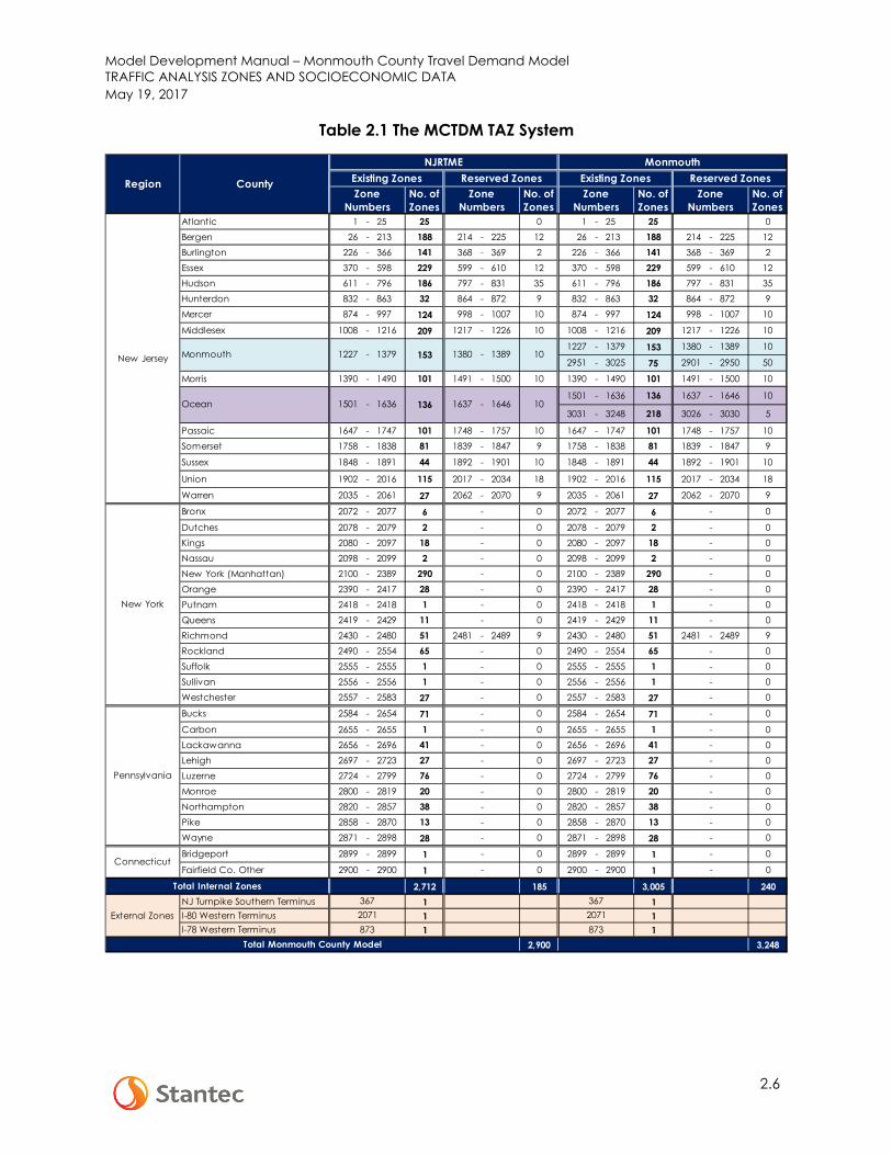
The MCTDM TAZ system was developed based on the updated NJRTM-E TAZ system along with additional refinement in Monmouth and Ocean Counties. The TAZ boundary was developed using the block, block-group, and census-tract boundaries of the 2010 Census. The TAZs in Ocean County are identical with the Ocean County Transportation Model that was completed in 2015, while the TAZ refinement for Monmouth County was developed with guidance from County Staff. The refined TAZ System consists of 3248 zones, including 3 external zones and 362 reserved zones for future use. 228 of those zones are in Monmouth County. Figure 2.2 shows an overlay of NJRTM-E TAZ Systems in Monmouth and Ocean Counties. Table 2.1 shows the list of TAZs by County for the entire model area.
The reserved zones were prepared for future use. For example, a corridor study that requires additional TAZ refinement. The reserved zones can be used in this study without changing the TAZ numbering system. Modifying or changing the TAZ numbers would lead to erroneous model execution and results.
The three external zones were added as part of the NJRTM-E Refinement Project that was completed in 2015. The original NJRTM-E did not use any external zones, instead it provided enough buffer areas of additional counties surrounding the thirteen NJTPA’s counties from which external traffic was to be generated. While the buffer area surrounding the NJTPA region is providing a reasonable external trip process for most of the modeled area, the estimated traffic on the southern section of the New Jersey Turnpike (NJTPK) were much lower than the observed traffic. An external zone representing the southern terminus of the NJTPK was added during the NJRTM-E Refinement Project to address this issue. Two additional external zones were also added at the western terminus of I-80 and I-78. It should be noted that the since the model has a larger buffer to the west and north of the NJTPA region, there is less traffic from these two external loading points reaching the NJTPA region than the traffic from the southern terminus of the NJTPK.

Model Development Manual – Monmouth County Travel Demand Model TRAFFIC ANALYSIS ZONES AND SOCIOECONOMIC DATA May 19, 2017
2.5
Figure 2.2 TAZ System in Monmouth County Region
Model Development Manual – Monmouth County Travel Demand Model TRAFFIC ANALYSIS ZONES AND SOCIOECONOMIC DATA May 19, 2017
2.6
Table 2.1 The MCTDM TAZ System
No. of Zones
No. of Zones
No. of Zones
No. of Zones
Atlantic 1 - 25 25 0 1 - 25 25 0Bergen 26 - 213 188 214 - 225 12 26 - 213 188 214 - 225 12Burlington 226 - 366 141 368 - 369 2 226 - 366 141 368 - 369 2Essex 370 - 598 229 599 - 610 12 370 - 598 229 599 - 610 12Hudson 611 - 796 186 797 - 831 35 611 - 796 186 797 - 831 35Hunterdon 832 - 863 32 864 - 872 9 832 - 863 32 864 - 872 9Mercer 874 - 997 124 998 - 1007 10 874 - 997 124 998 - 1007 10
Middlesex 1008 - 1216 209 1217 - 1226 10 1008 - 1216 209 1217 - 1226 10
1227 - 1379 153 1380 - 1389 10
2951 - 3025 75 2901 - 2950 50
Morris 1390 - 1490 101 1491 - 1500 10 1390 - 1490 101 1491 - 1500 10
1501 - 1636 136 1637 - 1646 10
3031 - 3248 218 3026 - 3030 5
Passaic 1647 - 1747 101 1748 - 1757 10 1647 - 1747 101 1748 - 1757 10Somerset 1758 - 1838 81 1839 - 1847 9 1758 - 1838 81 1839 - 1847 9
Sussex 1848 - 1891 44 1892 - 1901 10 1848 - 1891 44 1892 - 1901 10
Union 1902 - 2016 115 2017 - 2034 18 1902 - 2016 115 2017 - 2034 18
Warren 2035 - 2061 27 2062 - 2070 9 2035 - 2061 27 2062 - 2070 9
Bronx 2072 - 2077 6 - 0 2072 - 2077 6 - 0
Dutches 2078 - 2079 2 - 0 2078 - 2079 2 - 0Kings 2080 - 2097 18 - 0 2080 - 2097 18 - 0Nassau 2098 - 2099 2 - 0 2098 - 2099 2 - 0New York (Manhattan) 2100 - 2389 290 - 0 2100 - 2389 290 - 0Orange 2390 - 2417 28 - 0 2390 - 2417 28 - 0Putnam 2418 - 2418 1 - 0 2418 - 2418 1 - 0Queens 2419 - 2429 11 - 0 2419 - 2429 11 - 0Richmond 2430 - 2480 51 2481 - 2489 9 2430 - 2480 51 2481 - 2489 9Rockland 2490 - 2554 65 - 0 2490 - 2554 65 - 0Suffolk 2555 - 2555 1 - 0 2555 - 2555 1 - 0Sullivan 2556 - 2556 1 - 0 2556 - 2556 1 - 0Westchester 2557 - 2583 27 - 0 2557 - 2583 27 - 0
Bucks 2584 - 2654 71 - 0 2584 - 2654 71 - 0
Carbon 2655 - 2655 1 - 0 2655 - 2655 1 - 0Lackawanna 2656 - 2696 41 - 0 2656 - 2696 41 - 0Lehigh 2697 - 2723 27 - 0 2697 - 2723 27 - 0Luzerne 2724 - 2799 76 - 0 2724 - 2799 76 - 0Monroe 2800 - 2819 20 - 0 2800 - 2819 20 - 0Northampton 2820 - 2857 38 - 0 2820 - 2857 38 - 0Pike 2858 - 2870 13 - 0 2858 - 2870 13 - 0Wayne 2871 - 2898 28 - 0 2871 - 2898 28 - 0
Bridgeport 2899 - 2899 1 - 0 2899 - 2899 1 - 0
Fairfield Co. Other 2900 - 2900 1 - 0 2900 - 2900 1 - 0
2,712 185 3,005 240NJ Turnpike Southern Terminus 1 1I-80 Western Terminus 1 1I-78 Western Terminus 1 1
2,900 3,248
Total Internal Zones
NJRTME
101646-16371361636-
Monmouth
New York
Pennsylvania
Connecticut
New Jersey Monmouth
Ocean
Zone Numbers
Zone Numbers
Region County Existing Zones Reserved Zones Existing Zones Reserved Zones
1227 - 1379 153 1380 101389-
Zone Numbers
Zone Numbers
1501
2071873
367
Total Monmouth County Model
External Zones3672071873

Model Development Manual – Monmouth County Travel Demand Model TRAFFIC ANALYSIS ZONES AND SOCIOECONOMIC DATA May 19, 2017
2.7
2.3 SOCIOECONOMIC DATA
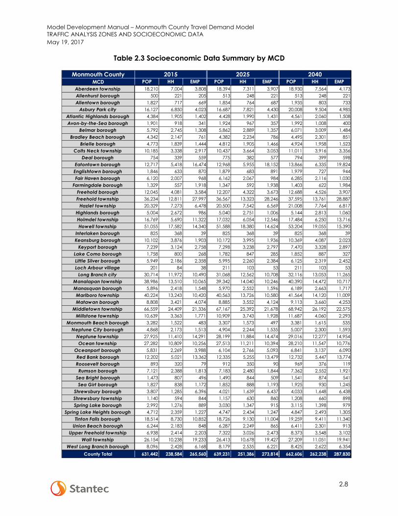
The socioeconomic data (SED) for the MCTDM was provided by NJTPA and it is consistent with SED that is utilized for the 2015 NJRTM-E Revalidation Project and expected to be used for NJTPA’s 2045 Regional Transportation Plan. As part of this three model-year scenarios have been prepared; 2015 (calibration year), 2025 and 2040. Table 2.2 shows the population (POP), household (HH), and employment (EMP) summary by county for the full model’s extent. Table 2.3 shows the summary by municipalities (MCD) for the Monmouth County Region and Table 2.4 presents the compounded annual growth rate (CAGR) between 2015-2025 and 2025-2040. The Monmouth County population and households are estimated to grow at an annual rate of 0.12% and 0.52%, respectively, between 2015 and 2025, while employment grows at a rate of 0.31% annually. Between 2025 and 2040, population and households are estimated to grow at a rate of 0.24% and 0.28% per year, respectively, while employment is estimated to grow at a rate of 0.33% per year.
Table 2.2 Socioeconomic Data Summary by County
2015 2025 2040 2015 2025 2040 2015 2025 2040Atlantic 269,939 286,821 312,144 102,250 108,644 118,236 164,953 167,260 170,721 Bergen 928,736 951,196 1,011,159 339,860 356,064 375,917 444,410 469,825 495,158 Burlington 450,912 471,735 494,722 168,000 177,175 186,644 218,492 228,427 239,422 Essex 790,286 818,044 885,615 289,757 306,636 335,761 372,712 392,071 417,641 Hudson 664,766 696,939 784,871 259,460 277,029 317,032 292,804 320,252 347,051 Hunterdon 127,964 128,443 133,892 48,489 51,016 52,722 55,827 57,304 60,638 Mercer 367,662 377,426 390,730 134,065 138,555 144,036 267,528 276,216 286,083 Middlesex 829,266 862,805 942,881 284,658 302,001 333,200 397,998 418,521 447,748 Monmouth 631,442 639,231 662,606 238,584 251,386 262,238 265,560 273,814 287,830 Morris 500,519 515,015 527,355 186,604 197,862 203,040 303,983 316,741 326,097 Ocean 585,735 629,601 727,411 225,056 243,084 282,784 169,467 183,536 201,414 Passaic 505,892 528,416 584,980 170,877 181,445 201,022 189,774 200,796 213,823 Somerset 331,195 339,637 359,896 118,200 126,293 134,632 192,717 203,308 216,146 Sussex 149,798 151,373 156,225 56,688 59,351 61,624 43,621 45,340 47,252 Union 549,162 572,196 633,168 189,424 199,433 220,062 245,932 257,616 273,198 Warren 109,881 112,152 117,200 42,989 45,655 48,541 36,043 37,630 39,270 Bronx 1,369,017 1,438,559 1,532,536 494,510 519,622 553,571 386,605 402,695 424,011 Dutchess 281,430 291,719 314,973 112,123 119,799 129,718 118,868 126,343 137,069 Kings 2,567,223 2,670,642 2,804,914 953,490 991,903 1,041,777 865,022 895,593 939,005 Nassau 1,331,352 1,356,323 1,503,550 450,947 468,171 511,890 578,075 596,938 630,461 New York 1,543,334 1,594,211 1,624,236 776,333 801,935 817,044 2,385,359 2,463,108 2,576,985 Orange 373,355 404,327 476,678 132,785 147,608 174,450 145,299 155,842 172,119 Putnam 97,432 98,824 105,090 36,187 38,231 40,290 28,529 29,090 29,393 Queens 2,261,478 2,325,428 2,384,645 801,323 823,972 844,957 727,389 741,692 760,688 Richmond 470,523 485,599 493,266 168,976 174,385 177,146 138,588 142,688 148,033 Rockland 315,895 328,990 370,167 103,962 108,891 121,928 118,415 127,409 139,808 Suffolk 1,471,420 1,509,850 1,626,165 508,497 541,575 588,165 637,685 673,361 721,640 Westchester 942,765 967,338 1,074,537 356,763 372,890 411,415 439,406 457,380 481,197 Bucks 634,887 673,289 727,145 240,202 257,429 279,557 296,107 313,849 335,697 Carbon 62,839 64,062 64,174 25,140 25,629 25,674 18,063 18,076 18,095 Lackawanna 212,771 210,447 210,086 85,927 85,028 84,863 97,399 96,540 95,268 Lehigh 367,603 406,436 469,975 143,340 161,139 185,574 234,009 262,324 302,771 Luzerne 301,158 296,045 295,655 122,422 120,009 119,819 143,073 140,251 136,112 Monroe 201,799 245,644 318,350 71,603 86,985 112,471 71,616 87,839 117,848 Northampton 313,625 347,641 403,979 121,003 135,626 156,703 139,093 155,149 176,761 Pike 80,304 106,075 153,938 30,024 39,659 57,554 12,100 15,864 23,303 Wayne 57,110 60,697 60,485 21,801 23,113 23,038 18,272 18,728 19,433
1,011,107 1,073,715 1,129,735 362,456 401,582 403,562 450,478 770,058 871,699 24,061,581 25,036,891 26,869,133 8,974,772 9,466,808 10,138,657 11,711,272 12,539,475 13,326,887
OthersTOTAL
HH EMPSTATE COUNTY POP
New
Jer
sey
New
Yor
kPe
nnsy
lvan
ia
Model Development Manual – Monmouth County Travel Demand Model TRAFFIC ANALYSIS ZONES AND SOCIOECONOMIC DATA May 19, 2017
2.8
Table 2.3 Socioeconomic Data Summary by MCD
Monmouth CountyMCD POP HH EMP POP HH EMP POP HH EMP
Aberdeen township 18,210 7,004 3,808 18,394 7,311 3,907 18,930 7,564 4,173Allenhurst borough 500 221 205 513 248 221 513 248 221Allentown borough 1,827 717 669 1,854 764 687 1,935 803 733
Asbury Park city 16,127 6,850 4,023 16,687 7,821 4,430 20,008 9,504 4,985Atlantic Highlands borough 4,384 1,905 1,402 4,428 1,990 1,431 4,561 2,060 1,508Avon-by-the-Sea borough 1,901 918 341 1,924 967 357 1,992 1,008 400
Belmar borough 5,792 2,745 1,308 5,862 2,889 1,357 6,071 3,009 1,484Bradley Beach borough 4,342 2,147 761 4,382 2,234 786 4,495 2,301 851
Brielle borough 4,773 1,839 1,444 4,812 1,905 1,466 4,924 1,958 1,523Colts Neck township 10,185 3,338 2,917 10,437 3,664 3,053 11,011 3,916 3,356
Deal borough 754 339 559 775 382 577 794 399 598Eatontown borough 12,717 5,418 16,474 12,968 5,955 18,152 13,866 6,335 19,824Englishtown borough 1,846 633 870 1,879 683 891 1,979 727 944Fair Haven borough 6,120 2,007 968 6,162 2,067 984 6,285 2,116 1,030
Farmingdale borough 1,329 557 1,918 1,347 592 1,938 1,403 622 1,984Freehold borough 12,045 4,081 3,584 12,207 4,322 3,673 12,688 4,526 3,907Freehold township 36,234 12,811 27,997 36,567 13,323 28,246 37,595 13,761 28,887
Hazlet township 20,329 7,273 6,478 20,500 7,542 6,569 21,008 7,764 6,817Highlands borough 5,004 2,672 986 5,040 2,751 1,006 5,144 2,813 1,060Holmdel township 16,769 5,690 11,322 17,032 6,054 12,546 17,484 6,250 13,716Howell township 51,055 17,582 14,340 51,588 18,380 14,624 53,204 19,055 15,390
Interlaken borough 825 368 39 825 368 39 825 368 39Keansburg borough 10,102 3,876 1,903 10,172 3,995 1,936 10,369 4,087 2,023
Keyport borough 7,239 3,124 2,758 7,298 3,238 2,797 7,470 3,328 2,897Lake Como borough 1,758 800 268 1,782 847 285 1,852 887 327Little Silver borough 5,949 2,186 2,358 5,995 2,260 2,384 6,125 2,319 2,452Loch Arbour village 201 84 38 211 103 53 211 103 53
Long Branch city 30,714 11,972 10,490 31,068 12,562 10,708 32,116 13,053 11,265Manalapan township 38,986 13,510 10,065 39,342 14,040 10,246 40,390 14,472 10,717Manasquan borough 5,896 2,418 1,548 5,970 2,552 1,596 6,189 2,663 1,717Marlboro township 40,224 13,243 10,420 40,563 13,726 10,580 41,564 14,120 11,009Matawan borough 8,808 3,421 4,074 8,885 3,552 4,124 9,113 3,660 4,253
Middletown township 66,559 24,409 21,336 67,167 25,392 21,678 68,942 26,192 22,575Millstone township 10,639 3,363 1,771 10,909 3,743 1,928 11,687 4,060 2,293
Monmouth Beach borough 3,282 1,522 483 3,307 1,573 497 3,381 1,615 535Neptune City borough 4,868 2,173 1,513 4,904 2,244 1,535 5,007 2,300 1,593
Neptune township 27,925 11,410 14,291 28,199 11,884 14,474 29,016 12,277 14,954Ocean township 27,282 10,809 10,256 27,513 11,211 10,394 28,210 11,547 10,776
Oceanport borough 5,831 2,269 3,988 6,104 2,766 5,093 6,841 3,137 6,090Red Bank borough 12,202 5,021 13,362 12,335 5,255 13,479 12,732 5,447 13,774Roosevelt borough 893 320 79 912 350 90 969 376 119Rumson borough 7,121 2,388 1,813 7,183 2,480 1,844 7,362 2,552 1,921
Sea Bright borough 1,473 807 496 1,490 844 509 1,541 874 541Sea Girt borough 1,827 838 1,172 1,852 888 1,193 1,925 930 1,245
Shrewsbury borough 3,807 1,285 6,396 4,021 1,639 6,437 4,033 1,648 6,438Shrewsbury township 1,140 594 844 1,157 630 860 1,208 660 898Spring Lake borough 2,992 1,276 889 3,030 1,347 915 3,115 1,398 979
Spring Lake Heights borough 4,712 2,359 1,227 4,747 2,434 1,247 4,847 2,493 1,305Tinton Falls borough 18,514 8,730 10,852 18,726 9,130 11,004 19,259 9,411 11,340
Union Beach borough 6,244 2,183 848 6,287 2,249 865 6,411 2,301 913Upper Freehold township 6,938 2,414 2,203 7,322 3,026 2,473 8,373 3,548 3,102
Wall township 26,154 10,238 19,233 26,413 10,678 19,427 27,209 11,051 19,941West Long Branch borough 8,096 2,428 6,168 8,179 2,535 6,221 8,425 2,622 6,354
County Total 631,442 238,584 265,560 639,231 251,386 273,814 662,606 262,238 287,830
20402015 2025

Model Development Manual – Monmouth County Travel Demand Model TRAFFIC ANALYSIS ZONES AND SOCIOECONOMIC DATA May 19, 2017
2.9
Table 2.4 SED Growth Rate by MCD
Monmouth CountyMCD POP HH EMP POP HH EMP
Aberdeen township 0.10% 0.43% 0.26% 0.19% 0.23% 0.44%Allenhurst borough 0.26% 1.18% 0.76% 0.00% 0.00% 0.00%Allentown borough 0.15% 0.63% 0.26% 0.28% 0.34% 0.43%
Asbury Park city 0.34% 1.33% 0.97% 1.22% 1.31% 0.79%Atlantic Highlands borough 0.10% 0.44% 0.20% 0.20% 0.23% 0.35%Avon-by-the-Sea borough 0.12% 0.52% 0.48% 0.23% 0.27% 0.75%
Belmar borough 0.12% 0.51% 0.37% 0.23% 0.27% 0.60%Bradley Beach borough 0.09% 0.40% 0.32% 0.17% 0.20% 0.53%
Brielle borough 0.08% 0.36% 0.15% 0.15% 0.18% 0.25%Colts Neck township 0.24% 0.94% 0.46% 0.36% 0.44% 0.63%
Deal borough 0.28% 1.19% 0.32% 0.16% 0.30% 0.24%Eatontown borough 0.20% 0.95% 0.97% 0.45% 0.41% 0.59%Englishtown borough 0.18% 0.78% 0.24% 0.34% 0.41% 0.39%Fair Haven borough 0.07% 0.30% 0.16% 0.13% 0.16% 0.31%
Farmingdale borough 0.14% 0.61% 0.10% 0.27% 0.32% 0.16%Freehold borough 0.13% 0.58% 0.25% 0.26% 0.31% 0.41%Freehold township 0.09% 0.39% 0.09% 0.19% 0.22% 0.15%
Hazlet township 0.08% 0.36% 0.14% 0.16% 0.19% 0.25%Highlands borough 0.07% 0.29% 0.20% 0.14% 0.15% 0.35%Holmdel township 0.16% 0.62% 1.03% 0.17% 0.21% 0.60%Howell township 0.10% 0.44% 0.20% 0.21% 0.24% 0.34%
Interlaken borough 0.00% 0.00% 0.00% 0.00% 0.00% 0.00%Keansburg borough 0.07% 0.30% 0.17% 0.13% 0.15% 0.29%
Keyport borough 0.08% 0.36% 0.14% 0.16% 0.18% 0.24%Lake Como borough 0.13% 0.58% 0.60% 0.26% 0.31% 0.92%Little Silver borough 0.08% 0.34% 0.11% 0.14% 0.17% 0.19%Loch Arbour village 0.47% 2.12% 3.41% 0.00% 0.00% 0.00%
Long Branch city 0.11% 0.48% 0.21% 0.22% 0.26% 0.34%Manalapan township 0.09% 0.39% 0.18% 0.18% 0.20% 0.30%Manasquan borough 0.13% 0.54% 0.30% 0.24% 0.28% 0.49%Marlboro township 0.08% 0.36% 0.15% 0.16% 0.19% 0.27%Matawan borough 0.09% 0.38% 0.12% 0.17% 0.20% 0.21%
Middletown township 0.09% 0.40% 0.16% 0.17% 0.21% 0.27%Millstone township 0.25% 1.08% 0.86% 0.46% 0.54% 1.16%
Monmouth Beach borough 0.08% 0.33% 0.28% 0.15% 0.17% 0.50%Neptune City borough 0.07% 0.32% 0.14% 0.14% 0.16% 0.25%
Neptune township 0.10% 0.41% 0.13% 0.19% 0.22% 0.22%Ocean township 0.08% 0.37% 0.13% 0.17% 0.20% 0.24%
Oceanport borough 0.46% 2.00% 2.47% 0.76% 0.84% 1.20%Red Bank borough 0.11% 0.46% 0.09% 0.21% 0.24% 0.14%Roosevelt borough 0.21% 0.90% 1.36% 0.40% 0.48% 1.88%Rumson borough 0.09% 0.38% 0.17% 0.16% 0.19% 0.28%
Sea Bright borough 0.12% 0.45% 0.25% 0.23% 0.23% 0.41%Sea Girt borough 0.13% 0.58% 0.18% 0.26% 0.31% 0.28%
Shrewsbury borough 0.55% 2.47% 0.06% 0.02% 0.04% 0.00%Shrewsbury township 0.14% 0.59% 0.19% 0.29% 0.31% 0.28%Spring Lake borough 0.13% 0.54% 0.28% 0.18% 0.25% 0.46%
Spring Lake Heights borough 0.07% 0.31% 0.17% 0.14% 0.16% 0.30%Tinton Falls borough 0.11% 0.45% 0.14% 0.19% 0.20% 0.20%
Union Beach borough 0.07% 0.30% 0.20% 0.13% 0.15% 0.36%Upper Freehold township 0.54% 2.29% 1.17% 0.90% 1.07% 1.52%
Wall township 0.10% 0.42% 0.10% 0.20% 0.23% 0.17%West Long Branch borough 0.10% 0.43% 0.09% 0.20% 0.23% 0.14%
County Total 0.12% 0.52% 0.31% 0.24% 0.28% 0.33%
2015-2025 2025-2040

Model Development Manual – Monmouth County Travel Demand Model TRAFFIC ANALYSIS ZONES AND SOCIOECONOMIC DATA May 19, 2017
2.10
This Page Is Intentionally Left Blank

Model Development Manual – Monmouth County Travel Demand Model DATA COLLECTION AND SOURCES May 19, 2017
3.1
3.0 DATA COLLECTION AND SOURCES
Data to support model calibration and validation efforts for various model components were gathered from numerous sources, including:
• 2010-2011 NJTPA and NYMTC Regional Household Travel Survey (RHTS). • 2010 census data and American Community Survey (ACS) data. • Longitudinal Employer-Household Dynamics (LEHD) data. • Monmouth and Ocean County Automatic Traffic Recorders (ATRs) counts. • NJDOT traffic counts Weigh-in-Motion (WIM) Data, and 48-hour continuous data. • New Jersey Turnpike Authority (NJTA) traffic counts along the Garden State Parkway. • INRIX speed data. • The 2015 NJ Transit Ridership data. • Ferry ridership data.
3.1 2010-2011 NJTPA-NYMTC RHTS DATA
The 2010-2011 RHTS was conducted from September 2010 through November 2011 in a coordinated effort between NJTPA and NYMTC. In total, 18,965 households completed the survey’s travel diaries, 7,574 of which were households in the NJTPA region. The survey study area comprises 28-counties constituting the Tri-State metropolitan area that includes:
• New York: Bronx, Dutchess, Kings, Nassau, New York, Orange, Putnam, Queens, Richmond, Rockland, Suffolk, and Westchester.
• New Jersey: Bergen, Essex, Hudson, Hunterdon, Mercer, Middlesex, Monmouth, Morris, Ocean, Passaic, Somerset, Sussex, Union, and Warren.
• Connecticut: Fairfield and New Haven.
The survey datasets are comprised of 18,965 household records, 39,789 person records, and 143,925 trip records. Of these records, only 679 households were from the Monmouth County Region. The sample represents approximately 0.3% of the total households in the region as shown in Table 3.1. The percentage of the sample size for Monmouth County is consistent with the sample size for the NJTPA region, the NJTPA’s 13 counties, as shown in Table 3.2. Figure 3.1 shows the sample size and location for Monmouth County. The household sample size by municipality is provided in Table 3.3.
Table 3.1 RHTS Sample Size for Monmouth County
Type Number of Samples SED (2015) % Sample
Household 679 238,584 0.3%

Model Development Manual – Monmouth County Travel Demand Model DATA COLLECTION AND SOURCES May 19, 2017
3.2
Table 3.2 RHTS Sample Size for NJTPA Counties
Figure 3.1 RHTS Sample Size by Location in Monmouth County
Type Number of Samples SED (2015) % Sample
Household 7,574 2,450,644 0.3%

Model Development Manual – Monmouth County Travel Demand Model DATA COLLECTION AND SOURCES May 19, 2017
3.3
Table 3.3 RHTS Sample Size by Municipality
3.2 LONGITUDINAL EMPLOYER-HOUSEHOLD DYNAMICS DATA
The Longitudinal Employer-Household Dynamics (LEHD) data is published by the Center for Economic Studies at the US Census Bureau. The LEHD data provides information such as household and employer locations that can be used as a complimentary data source for calibrating trip distribution of the Home-Based Trip Purpose (HBW). The latest LEHD data available was collected in 2014. Additional discussion on the LEHD data will be provided in the Trip Distribution Calibration Section (Section 9.3).
Monmouth MCD Number of Samples Monmouth MCD Number of
SamplesAberdeen township 11 Long Branch city 8 Allenhurst borough - Manalapan township 47 Allentown borough - Manasquan borough 5
Asbury Park city 3 Marlboro township 58 Atlantic Highlands borough 2 Matawan borough 5 Avon-by-the-Sea borough 2 Middletown township 250
Belmar borough 2 Millstone township 5 Bradley Beach borough 1 Monmouth Beach borough -
Brielle borough 7 Neptune City borough 2 Colts Neck township 8 Neptune township 27
Deal borough - Ocean township 35 Eatontown borough 6 Oceanport borough - Englishtown borough 2 Red Bank borough 1 Fair Haven borough 12 Roosevelt borough -
Farmingdale borough 1 Rumson borough 11 Freehold borough 2 Sea Bright borough - Freehold township 10 Sea Girt borough -
Hazlet township 13 Shrewsbury borough 2 Highlands borough 6 Shrewsbury township 1 Holmdel township 3 Spring Lake borough 6 Howell township 60 Spring Lake Heights borough 7
Interlaken borough - Tinton Falls borough 7 Keansburg borough 26 Union Beach borough 1
Keyport borough 10 Upper Freehold township 1 Lake Como borough - Wall township 7 Little Silver borough - West Long Branch borough 6 Loch Arbour village -
679 Total

Model Development Manual – Monmouth County Travel Demand Model DATA COLLECTION AND SOURCES May 19, 2017
3.4
3.3 TRAFFIC COUNT DATA
The traffic count data was obtained from various sources, including:
• Traffic count data provided by Monmouth County • Traffic count data that was collected in the past three years from Ocean County • Garden State Parkway and the New Jersey Turnpike traffic count data obtained from the
New Jersey Turnpike Authority (NJTPA) • Traffic count data downloaded from the NJDOT’s website.
As part of this project, Stantec gathered traffic count data between 2013 and 2017. All the counts that were collected on the years other than 2015 were converted into 2015 counts, the model calibration year, using assumed growth rate derived from various permanent station locations within Monmouth County. Table 3.4 shows the assumed annual growth factor of 0.6% used for this purpose.
Table 3.4 Average Annual Growth Rates
Considering that the County Model is calibrated to the average annual weekday traffic (AWDT), the count data that were based on the average annual daily traffic (AADT) shall be converted into AWDT. Stantec developed the AWDT factors using the same permanent count data used for estimating the annual growth rates above. Table 3.5 shows the AADT to AWDT conversion factor.
COUNTY SITE NAME FACILITY TYPE/LOCATION2015
TRAFFIC VOLUME
ANNUAL GROWTH
RATE6-1-002 Rural Principal Arterial - Other (Rt. 33 - Wall TWP) 39,722 1.7%6-1-010 Rural Principal Arterial - Other (Rt. 33 - Manalapan TWP) 27,649 -2.1%6-1-011 Urban Principal Arterial - Other (Rt. 18 - Marlboro TWP) 51,210 0.3%6-1-014 Urban Collector (Old Mill Road - Sring Lake Height Boro) 2,986 4.4%6-1-015 Rural Principal Arterial - Interstate (I-195 - Upper Freehold) 53,991 3.0%6-1-016 Urban Principal Arterial - Other Freeways (Rt. 138 - Wall TWP) 23,366 1.4%6-1-017 Urban Principal Arterial - Other (NJ 34 - Wall TWP) 31,098 1.4%6-1-018 Rural Minor Arterial (NJ 34 - Wall TWP) 34,978 -1.6%6-1-020 Urban Principal Arterial Other (NJ 36 - Sea Bright Boro) 11,485 -4.5%6-1-022 Urban Principal Arterial - Other (Freehold TWP) 53,267 -0.2%6-1-024 Rural Principal Other (NJ 18 - Colts Neck Twp) 40,274 1.1%
0.6%
Monmouth
Average Growth Rate Per Year

Model Development Manual – Monmouth County Travel Demand Model DATA COLLECTION AND SOURCES May 19, 2017
3.5
Table 3.5 AADT TO AWDT CONVERSION FACTOR
For the purpose of the screenline calibration, additional traffic counts were collected at fourteen locations specified by Monmouth County, mostly at the locations along the screenlines, as shown in Table 3.6. All traffic count locations used in the model calibration are shown in Figure 3.2. Roadway links where traffic counts are available are printed in green in this Figure. Traffic counts from the adjacent counties, such as Burlington, Middlesex, and Ocean, in the vicinity of Monmouth County are also available and will be used for the calibration.
Table 3.6 Additional Traffic Count Locations
COUNTY SITE NAME FACILITY TYPE/LOCATION AWDT AADT FACTOR6-1-002 Rural Principal Arterial - Other (Rt. 33 - Wall TWP) 39,722 38,736 1.036-1-010 Rural Principal Arterial - Other (Rt. 33 - Manalapan TWP) 27,649 26,445 1.056-1-011 Urban Principal Arterial - Other (Rt. 18 - Marlboro TWP) 51,210 48,556 1.056-1-014 Urban Collector (Old Mill Road - Sring Lake Height Boro) 2,986 2,935 1.026-1-015 Rural Principal Arterial - Interstate (I-195 - Upper Freehold) 53,991 53,469 1.016-1-016 Urban Principal Arterial - Other Freeways (Rt. 138 - Wall TWP) 23,366 23,224 1.016-1-017 Urban Principal Arterial - Other (NJ 34 - Wall TWP) 31,098 28,540 1.096-1-018 Rural Minor Arterial (NJ 34 - Wall TWP) 34,978 34,193 1.026-1-020 Urban Principal Arterial Other (NJ 36 - Sea Bright Boro) 11,485 11,312 1.026-1-022 Urban Principal Arterial - Other (Freehold TWP) 53,267 52,004 1.026-1-024 Rural Principal Other (NJ 18 - Colts Neck Twp) 40,274 37,667 1.07
1.04
Monmouth
AADT TO AWDT CONVERSION FACTOR
Location Number Street Name Description
1 NJ-35 Between Navesink River Rd and Cooper Rd2 Broadway Between Norwood Ave and 3rd Ave3 Sea Girt Ave (E of Old Mill Rd) Between Old Mill Rd and NJ-714 Five Points Rd Between CR-537 and NJ-185 CR-12A W of Browns Dock Rd6 CR 15 Grassmere Ave Between Westra St and Main St7 Ely Harmony Rd Between Siloam Rd and Nomoco Rd8 Wilson Ave Between Texas Rd and NJ-799 Kings Hwy E Between Chapel Hill Rd and Locust Point Rd
10 Wickapecko Dr Between Roseld Ave and NJ-6611 Bangs Ave Between Ridge Ave and NJ-7112 N Bath Ave (SE of High St) Between Norwood Ave and 3rd Ave13 Westwood Ave (S of N Bath Ave) Between N Bath Ave and Cedar Ave14 Ely Harmony Rd Between CR-537 and Siloam Rd

Model Development Manual – Monmouth County Travel Demand Model DATA COLLECTION AND SOURCES May 19, 2017
3.6
Figure 3.2 All Traffic Count Locations in Monmouth County
3.4 SPEED DATA
Speed data along various roadways within the Monmouth County region will be used as part of the highway assignment calibration. The data can be used for comparison with the model estimated speed. Depending on this comparison, the adjustments to the assumed speed and roadway capacity can be performed to bring the estimated speed closer to the observed speed. The observed speed data that will be used in the model calibration was obtained from INRIX data and provided by NJTPA. The observed speed data at various locations are shown in Table 3.7.

Model Development Manual – Monmouth County Travel Demand Model DATA COLLECTION AND SOURCES May 19, 2017
3.7
Table 3.7 Observed Speed Data from INRIX
3.5 TRANSIT RIDERSHIP DATA
Transit trips in Monmouth County only account for 2.8% of overall trips generated in the county, as revealed by the Household Survey Data. Those trips are mostly served by NJ Transit buses and commuter trains, but also included travel modes such as ferries and private buses. NJ TRANSIT provided the 2015 bus and rail daily ridership data, while Monmouth County provided the ferry data. Unfortunately, ridership on the 800 series buses is not available. Table 3.8 lists the observed daily ridership data by transit mode.
AM MD PM NTNorthbound 68 68 68 66Southbound 69 68 66 67Northbound 40 35 33 42Southbound 40 35 33 41Westbound 67 67 66 66Eastbound 67 67 68 66Westbound 46 47 45 48Eastbound 47 47 45 48
Northbound 66 63 65 63Southbound 64 64 65 63Northbound 32 30 28 34Southbound 33 30 28 34Northbound 32 33 31 35Southbound 34 34 31 37Northbound 43 42 40 45Southbound 42 42 39 44Westbound 38 36 33 40Eastbound 38 37 35 40
Between I-195 and GSP
Location Observed Average Speed (INRIX Data)
Between NJ TPK and RT 18
Between US 9 and CR 33
Between US 9 and County Line Rd.
Between RT 34 and RT 33
Between RT 79 and RT 35
CR 33
RT 537
RT 34
RT 79
CR 35
RT 18
Garden State Parkway
US 9
I-195
Road Name Direction
Between US 9 and Burnt Tavern Rd
Between RT 18 and Central Avenue
Between NJ TPK and GSP

Model Development Manual – Monmouth County Travel Demand Model DATA COLLECTION AND SOURCES May 19, 2017
3.8
Table 3.8 Observed Daily Ridership by Transit Mode
Terminal Ferry RidershipBelford 1,916
Atlantic Highlands 1,863Highlands 1,417
Total 5,195
Train Station Rail RidershipAberdeen-Matawan 2,460
Hazlet 874Middletown 1,331Red Bank 1,155
Little Silver 740
Long Branch 1,105Elberon 117
Allenhurst 125Asbury Park 548
Bradley Beach 225Belmar 256
Spring Lake 152Manasquan 175
Total 9,263
Line No. Bus Ridership Route63 85 Lakewood- Jersey City - Weehauken64 762 Lakewood – Jersey City - Weehawken67 496 Toms River – Newark – Jersey City
130 763 Lakewood – New York Express (Outbound)
131 555 Sayreville – New York132 329 Lakewood - Gordon's Corner – New York133 617 Old Bridge – Aberdeen – New York135 359 Freehold – Matawan – New York
136 157 Lakewood - Freehold Mall - New York Express137 1,017 Toms River - New York139 6,127 Lakewood – New York317 437 Asbury Park – Fort Dix – Philadelphia319 345 Atlantic City – New York
Total 12,049

Model Development Manual – Monmouth County Travel Demand Model HIGHWAY NETWORK DEVELOPMENT May 19, 2017
4.1
4.0 HIGHWAY NETWORK DEVELOPMENT
4.1 INTRODUCTION
The MCTDM highway network was developed based on the NJRTM-E highway network with additional roadway refinement within Monmouth and Ocean counties. Many local roadways were added to the highway network to provide more detail representation of the roadways in these two counties. Figure 4.1 shows the highway network refinements made within Monmouth and Ocean Counties compared to the NJRTM-E highway network.
Figure 4.1 MCTDM Highway Network Refinements

Model Development Manual – Monmouth County Travel Demand Model HIGHWAY NETWORK DEVELOPMENT May 19, 2017
4.2
This section provides a detailed description of the highway network development task for the MCTDM project. The MCTDM highway network includes most of the major arterials and collector roads in the county to help represent travel in the region. The highway network includes variables such as travel time and toll costs that will be used as the basis for estimating composite impedance variables, which in turn will be used by the trip distribution model. The composite impedance variable will be discussed further in Chapter 8.
The highway network is developed as a series of links and nodes with the links representing roadway segments and the nodes representing their point of intersection. The highway network also includes zone centroids which serve as terminal points for trips in the modeling process. These zones centroids also represent proxy locations for the socioeconomic data (population and employment) contained within the TAZs that generate trips in the MCTDM. The centroids are attached to the highway network via hypothetical links called centroid connectors.
Each highway link contains data that define the operational and physical characteristics of the given facility along with fields used to provide identification data, such as roadway names. In general these parameters are categorized into three groups:
• Physical/operational variables • Identification variables • Performance variables
The complete list of these variables is given in Appendix A.
4.2 PHYSICAL/OPERATIONAL VARIABLES
These variables describe the physical and operational attributes of the highway network which help determine the capacity and speed of the links. The techniques used to estimate speed and capacity are based on the 2000 Highway Capacity Manual (HCM) procedures, published by the Transportation Research Board (TRB), and were implemented in order to provide sensitivity to a wider range of potential improvement types, such as signalization and intersection improvements, with the objective of providing more realistic estimates of capacity suitable for operational analysis. Several key variables will be discussed in the following sections including:
• Facility type • Area Type • Link Type • Number of Lanes by Time Period • Traffic Control Devices Variables • Toll Variables
Facility type and area type variables are used for defining speed and capacity for the links. Additional discussion on the link speed and capacity is presented in Section 4.2.8.

Model Development Manual – Monmouth County Travel Demand Model HIGHWAY NETWORK DEVELOPMENT May 19, 2017
4.3
4.2.1 Facility Type
The MCTDM recognizes twelve different facility types that are stored in the “FT” variable. The twelve facility categories are as follows:
• Freeways (FT=1) – limited access roadway facilities, including toll facilities, with grade-separated interchanges and no traffic signals on the main lanes. Example: Garden State Parkway, I-195.
• Expressway (FT=2) – partially limited access roadway facilities with generally high speed limits, grade separated interchanges with other major facilities, and at-grade intersections with minor facilities. Example: US-9 in Freehold Township.
• Principal Arterial Divided (FT=3) – arterials with moderately high speed limits (e.g. 35-50 mph), raised center medians with turning bays at intersections, parking restrictions, mainly serving through traffic rather than local property access. Example: NJ-33 in Freehold Township.
• Principal Arterial Undivided (FT=4) – same as principal arterial divided except that there are no raised center medians and, generally, no bays for left turns. Example: NJ-36 in Monmouth Beach.
• Major Arterial Divided (FT=5) – arterials with moderate speed limits (e.g. 30-45 mph), raised center median with turning bays at intersections, some parking restrictions, mainly serving through traffic although some local property access is permitted. No coded examples in Monmouth County.
• Major Arterial Undivided (FT=6) – same as major arterials divided except that there are no raised center medians and, generally, no bays for left turns. Example: CR-520 in Lincroft.
• Minor Arterial (FT=7) – arterials with moderately low speed (e.g. 25-35 mph) and few parking restrictions that serve some through traffic, some distribution of traffic from principal and major facilities to local streets and local property access. Example: CR3 – Tennent Road in Manalapan.
• Collectors/Locals (FT=8) – roadways with moderately low speed limit (e.g. 25-35 mph) and few parking restrictions that serve mainly to collect and distribute traffic from principal, major, and minor facilities to local streets and local property access. Example: CR4 – Crine Road in Colts Neck.
• High-Speed Ramps (FT=9) – ramps that generally connect freeway-to-freeway facilities, or also known as direct connector, have some relatively high speed limits, e.g. 50-60 mph.
• Medium-Speed Ramps (FT=10) – ramps that have moderately high turning radius and typically with speed limit approximately 40 mph.
• Low-Speed Ramps (FT=11) – ramps with low turning radius and low speed limit, e.g. 25 mph, includes jughandles.

Model Development Manual – Monmouth County Travel Demand Model HIGHWAY NETWORK DEVELOPMENT May 19, 2017
4.4
• Centroid Connectors (FT=12) – “dummy” roadway link with unlimited capacity that serve solely to connect TAZs to roadway network. These are only used by the model and do not reflect real world facilities.
4.2.2 Area Type
Four separate area types were identified for the purpose of estimating highway capacity and speeds. These types are stored in the “AT” variable. The four area types are as follows:
• CBD (AT=1) – this area type is designated particularly for areas where population and employment densities are typically very high, such as Manhattan, downtown Newark and Jersey City.
• Urban (AT=2) – characterized by high residential densities, small lots or single family dwelling units, many apartments, and mostly through streets. The area is characterized by a mix of land-uses including residential and commercial land-uses.
• Suburban (AT=3) – characterized by low to medium residential densities, medium to large lots for single family housing units, homogenous land uses, restricted traffic flow restrictions such as cul-de-sacs, dead ends, traffic circles, and frequent stop signs.
• Rural (AT=4) – characterized by very low residential densities and much undeveloped or agricultural land, relatively few roads.
The area type designation in Monmouth County is shown in Figure 4.2.

Model Development Manual – Monmouth County Travel Demand Model HIGHWAY NETWORK DEVELOPMENT May 19, 2017
4.5
Figure 4.2 Area Type Designation in Monmouth County
4.2.3 Link Type
This variable is used in the model as a permission code when assigning vehicles to access highway links based on a vehicle’s mode type (e.g., excluding trucks on auto only roads) and toll facility type (e.g., differentiating single and high occupancy vehicles for tolls). This variable is used in highway path building and highway assignment procedures. There are sixteen (16) link types defined in the MCTDM and they are listed below:
1. Free All (Link Type 1) – non-tolled links designated for all modes.
2. Free Auto Only (Link Type 2) – non-tolled links designated for auto mode only.
3. Free Truck Only (Link Type 3) – non-tolled links designated for truck mode only.
4. Urban Toll All (Link Type 4) – Urban tolled links designated for all trip modes (auto and trucks). Urban links are defined as links with Area Type 3 or higher (Area Types 1 to 3). The toll links are assumed to accommodate all types of toll payments, such as cash or electronic toll collection (ETC or EZ-Pass).
5. Urban Toll Auto Only (Link Type 5) – Urban tolled links designated for auto mode only.

Model Development Manual – Monmouth County Travel Demand Model HIGHWAY NETWORK DEVELOPMENT May 19, 2017
4.6
6. Urban Toll Truck Only (Link Type 6) – Urban tolled links designated for truck mode only.
7. Rural Toll All (Link Type 7) – Rural tolled links designated for all trip modes (auto and trucks).
8. Rural Toll Auto Only (Link Type 8) – Rural tolled links designated for auto mode only.
9. Rural Toll Truck Only (link Type 9) – Rural tolled links designated for truck mode only.
10. Urban Free HOV Only (Link Type 10) – Urban free links for all HOV modes. This is a typical HOV link.
11. Urban Toll HOV Only (Link Type 11) – Urban tolled HOV Only. This link type is prepared for a scenario where the HOV links are now tolled.
12. Urban Toll SOV, Free HOV (Link Type 12) – Urban tolled links for SOV mode only, HOV mode is free. This is a typical use for HOT Lane scenarios.
13. Urban Toll Non-HOV vehicles (Link Type 13) – Urban toll links, all vehicles except HOVs
14. ETC Only All (Link Type 14) – Toll links dedicated for ETC patrons only (patrons with EZ-pass) for all modes. This link type is typical for congestion pricing or HOT lane scenarios where all payments are done electronically.
15. ETC Only Auto Only (Link Type 15) – Toll links dedicated for ETC patrons and Auto mode only. Truck trips are not eligible to use this type of link.
16. ETC Only SOV and Truck Toll, HOV Free (Link Type 16) – Toll links dedicated for all ETC patrons; however, only SOV and truck trips must pay. HOV mode is free.
Note that the MCTDM creates a total of nine different path sets based on mode (SOV, HOV, Truck) and toll usage (Free, Cash Payment, ETC Payment). It is important to note that the Link Type variable does not assess the toll cost. It is only used to determine if a path set can use the link in question. For example, the path-building and highway assignment process for an SOV cash path without EZ-Pass should exclude all links with link types:
• 3, 6, 9 because these links are limited to trucks only • 10, 11 because these links are limited to HOVs only • 14, 15, and 16 because these links are limited to vehicles with transponders (ETC).
4.2.4 Number of Lanes
The model provides three number of lane variables by time of day:
• LanesAM – number of lanes for AM Peak period • LanesPM – number of lanes for PM Peak period • LanesOP – number of lanes for Midday and Night periods
The purpose of having different variables for each time period is to accommodate the situations where the configuration of the roadway varies by time of day, such as a period-specific HOV lane or a roadway with a reversible lane. Typically, an HOV lane is usually applied to the peak direction reducing one lane from the available general-purpose lanes. During the off-peak period, this lane

Model Development Manual – Monmouth County Travel Demand Model HIGHWAY NETWORK DEVELOPMENT May 19, 2017
4.7
is usually converted back into a general-purpose lane. Currently, there is no reversible lane in Monmouth County. Having separate lane variables for each time-period within a master network for each model year reduces the model complexity by providing a consistent network suitable for several different time-of-day analyses.
4.2.5 Traffic Control Devices
The traffic control device (TCD) parameters were added to the model to improve the representation of capacity, speed and intersection delay. The MCTDM provides 13 TCD categories, defined as follows:
• Two-way stop (TCD 1) • All-way stop (TCD 2) • Yield (TCD 3) • Ramp-meter (TCD 4) • Signalized-uncoordinated-actuated (TCD 5) • Signalized-uncoordinated-fixed (TCD 6) • Signalized-coordinated-restricted progression (TCD 7) • Signalized-coordinated-favorable progression (TCD 8) • Signalized-coordinated-maximum progression (TCD 9) • Freeway diverge point (TCD 10) • Freeway merge point (TCD 11) • No controls (TCD 12) • Unknown (TCD 99)
As mentioned previously, the techniques to estimate speed and capacity utilize this variable as part of the 2000 HCM procedures. In addition to TCD variable, the model also includes additional signal-related variables that adjust time and capacity. These variables include:
• NSIG – number of signals in the link • SIGCYC – Signal cycle in seconds • SIGCOR – Signal coordination type
0 = uncoordinated signal (default) 1 = coordinated-unfavorable 2 = coordinated-favorable 3 = coordinated-maximum progression
• GC – green time per cycle ratio
The detailed data for the TCD and its complimentary variables can be updated in the future as more comprehensive databases become available. Note that due to the implementation of a separate intersection model for Monmouth and Ocean Counties (see Section 4.2.6), and to prevent the double-counting of TCD modeling, the TCD variable for Monmouth County and Ocean County has been defined as TCD=12 (no controls). The impact of the TCD in these two counties are controlled by the junction model.
Model Development Manual – Monmouth County Travel Demand Model HIGHWAY NETWORK DEVELOPMENT May 19, 2017
4.8
4.2.6 Intersection Model
To improve the modeling of intersections, Citilabs, the developer of the Cube Software, introduced a module called Intersection Model. This module allows analysts to provide more detailed information for intersections in the model, such as type of intersection, traffic signal phasing, etc. The Intersection Model will convert all the intersections characteristics into turning penalties during the highway skim and highway assignment process. The turning penalty represents additional intersection delays caused by traffic control devices installed in an intersection. These delays will be added to link travel time during a highway path building and highway assignment process in selecting a shortest route between an origin point and a destination point.
While this module provides the ability to input detailed intersection information, since the MCTDM is still a macroscopic model, it is not a replacement for a microsimulation model for more detail corridor analysis. The Intersection Model recognizes several types of intersections, including:
• Signal-controlled intersections • Two-way stop • All-way stop • Roundabout • Priority junction (Yield)
Due to the limited availability of intersection data, Stantec developed default assumptions for each intersection type. These assumptions are included in Appendix B. The intersection data can always be updated in the future when the data is available. The Intersection Model is not used in the NJRTM-E, however, it is included in the Ocean County Transportation Model.
4.2.7 Toll Variables
The MCTDM requires several toll variables for different toll applications. The toll variables are listed below:
• TOLL – the toll cost values in dollars.
• MCTOLL – a variable indicating whether the toll is two-way (driver encounters it in both directions) or is charged only one-way on the facility (e.g., most bridges and tunnels to NYC are one-way tolls). This variable is used by the mode choice process. MCTOLL will be explained further following this list.
• TOLLAPC – a flag to identify the type of toll links, for example, HOV free toll links, truck-free toll links, etc. The TOLLAPC has three possible values.
o TOLLAPC=0: This is the default value. The toll is applied to all modes (SOV, HOV, and truck).
o TOLLAPC=1: The toll is applied to all modes, except HOV.

Model Development Manual – Monmouth County Travel Demand Model HIGHWAY NETWORK DEVELOPMENT May 19, 2017
4.9
o TOLLAPC=2: The toll is applied to all modes, except trucks.
• TOLLCLASS – toll class for lookup system. This variable provides flexibility to use toll values either directly from values coded in the link or values defined in a look-up table. A detailed discussion about the toll look-up table will be given following this list.
o TOLLCLASS=0: This is the default value. This is applied to all links without any toll values.
o TOLLCLASS between 1 and 98: The toll cost will be obtained from a look-up table.
o TOLLCLASS=99: The toll value is coded directly on the link.
• TOLLFACAM, TOLLFACPM, TOLLFACMD, TOLLFACNT – base toll factor for each time-period (AM, PM, MD, and NT). This variable provides flexibility to have variable tolls for different time periods. The default values of these variables are one (1), i.e., tolls are the same for all time periods and they are the same as the values coded in the toll links.
• FIXTOLL – this variable provides whether or not the toll cost is fixed through all assignment iterations, or can be adjusted for each assignment iteration such as for congestion pricing scenarios. The FIXTOLL variable has two values, a value 0 for variable tolls and a value of 1 for fixed toll rates. The default is fixed tolls.
MCTOLL variable is used to identify facilities with one-way tolling schemes and is used by both the mode choice and highway assignment processes. For mode choice, trips are processed in a production-attraction format and the choice of mode is based on cost and time considerations of each mode encountered on the trip from the production TAZ to the attraction TAZ. For estimating the highway trip cost, the model needs to assume that the toll is encountered at some time during the day (whether it’s the initial or the return trip. Therefore, this variable is used to split the round-trip cost of the one-way toll using 50% of the total one-directional toll for each direction of the facility However, for the purposes of traffic assignment, the full cost of the toll is posted in the direction that the toll is assessed. This allows for the potential of vehicles diverting their trip (free vs. toll) if such options are present. An example of this directional tolling schemes employed in Monmouth County and its vicinity is present on the Garden State Parkway. In this situation, travelers are able to move in one direction either toll free or paying fewer tolls than they would be on the opposition direction trip. Certain travelers can use the Garden State Parkway in the reduced toll direction, and return via other toll-free roadways.
The possible values for MCTOLL are as follows:
• MCTOLL=0: no toll on the link (the default value).
• MCTOLL=1 for links with the same toll value in both directions
• MCTOLL=+0.5 and -0.5 for links with a one-way toll. The positive value (+0.5) is posted on link in the direction where the one-way toll is assessed, while the negative value (-0.5) is posted on the reverse, non-toll direction.
Model Development Manual – Monmouth County Travel Demand Model HIGHWAY NETWORK DEVELOPMENT May 19, 2017
4.10
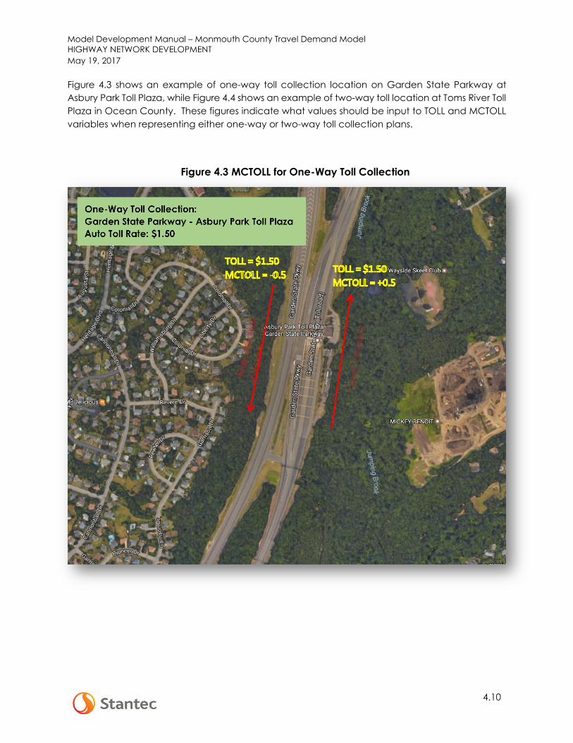
Figure 4.3 shows an example of one-way toll collection location on Garden State Parkway at Asbury Park Toll Plaza, while Figure 4.4 shows an example of two-way toll location at Toms River Toll Plaza in Ocean County. These figures indicate what values should be input to TOLL and MCTOLL variables when representing either one-way or two-way toll collection plans.
Figure 4.3 MCTOLL for One-Way Toll Collection

Model Development Manual – Monmouth County Travel Demand Model HIGHWAY NETWORK DEVELOPMENT May 19, 2017
4.11
Figure 4.4 MCTOLL for Two-Way Toll Collection
For one-way toll collection plan, the toll values for mode choice are the absolute values of the TOLL multiplied by MCTOLL. In the example above, both directions will have toll values of $0.75. In the assignment process, the assigned toll values will be the TOLL multiplied by a “factor”. The “factor” is defined as a one (1) if MCTOLL is greater than zero and defined as a zero (0) if MCTOLL is less or equal to zero. In the example above, the TOLL value for the toll direction (Northbound) is $1.50, while the TOLL value for the reverse direction is $0.00.
In contrast to the one-way toll collection plan at Asbury Park Plaza, the MCTOLL variable is coded differently to represent the two-way toll collection situation at Toms River, New Jersey. As shown in Figure 4.3, the MCTOLL variable is coded as “1” in each direction which enables the toll to be properly assessed for both mode choice and the highway assignment procedures. Note that an equal toll cost (in this case $0.75) is applied to each direction of the link, just as was the case with the one-directional toll scheme. It should also be noted that the MCTOLL variable can be used to identify the tolling locations for display purposes in CUBE and GIS by showing only those links where MCTOLL is greater than zero. This will display the actual toll in the direction that it is assessed.
TOLLCLASS, as explained previously, is a variable to allow the use of toll rates either directly coded on the link or toll rates defined from a look-up table. The look-up table that contains the toll rate is stored in “LOOKUPTOLLS.DBF” file in the “Highway Path-Building and Skim Estimation” module, as shown in Figure 4.5. Note that most, or if not all, of the toll rates in this model are posted directly on the links.

Model Development Manual – Monmouth County Travel Demand Model HIGHWAY NETWORK DEVELOPMENT May 19, 2017
4.12
Figure 4.5 Toll Class Look-Up Table
The MCTDM model reserves 98 keys (TOLLCLASS=1-98) to be used for different toll rates. Currently, only 12 keys have been populated, although not used. The remaining keys are reserved for future use. Note that TOLLCLASS code 99 is used to indicate that the lookup table is not applied and that the toll posted on the link is the actual value.

Model Development Manual – Monmouth County Travel Demand Model HIGHWAY NETWORK DEVELOPMENT May 19, 2017
4.13
4.2.8 Speed and Capacity Estimation
Speeds and capacity variables for the MCTDM were developed by using relationships between facility type and area type. The values adopted for this effort were obtained from several sources, including the speeds provided by the 2000 HCM procedures, and were adjusted using professional judgment during the course of the model development. The recommended “ideal” uncongested speeds (off-peak speed), which are used as input to the highway path building process, are presented in Table 4.1. Note that these speeds represent theoretical upper limits or “ideal” values prior to considering other factors such as number of lanes, grade, shoulder conditions, and traffic control devices that reduce these initial values. Initial estimates of congested speeds (peak speeds), which are used as input to first iteration of the highway path building process were assumed to be approximately 20% lower than the uncongested speed.
Table 4.1 Uncongested Speed by Facility Type and Area Type
The “ideal” capacities were also assumed to be a function of facility type and area type. These initial hourly capacities per lane are listed in Table 4.2. The initial capacity values for each link were adjusted to account for geometric constraints or other impedances along the link, such as parking availability, traffic control devices, green time/cycle ratio, signal cycle length, etc.
CBD Urban Suburban RuralFreeways 60 60 70 70Expressways 50 52 53 55Principal Arterials Divided 42 50 51 52Principal Arterials Undivided 40 40 45 48Major Arterials Divided 35 39 44 45Major Arterials Undivided 32 36 40 41Minor Arterials 25 29 32 33Collectors/Locals 20 25 26 26High-speed Ramps 50 52 53 55Medium-speed Ramps 30 30 30 30Low-speed Ramps 25 25 25 25Centroid Connectors 10 10 10 10
Area TypeFacility Type

Model Development Manual – Monmouth County Travel Demand Model HIGHWAY NETWORK DEVELOPMENT May 19, 2017
4.14
Table 4.2 Initial Hourly Capacity per Lane
The adjustments to speed and capacity are implemented during creation of period-specific networks and the procedures can be viewed in the control files in the “Highway Network Development Module” as shown in Figure 4.6.
CBD Urban Suburban RuralFreeways 1600 1650 1700 1750Expressways 1500 1525 1575 1625Principal Arterials Divided 1450 1525 1550 1600Principal Arterials Undivided 1400 1425 1500 1550Major Arterials Divided 1350 1375 1475 1500Major Arterials Undivided 1000 1025 1100 1150Minor Arterials 800 825 900 950Collectors/Locals 700 725 750 775High-speed Ramps 1750 1750 1750 1750Medium-speed Ramps 900 900 900 900Low-speed Ramps 700 700 700 700Centroid Connectors 9000 9000 9000 9000
Area TypeFacility Type

Model Development Manual – Monmouth County Travel Demand Model HIGHWAY NETWORK DEVELOPMENT May 19, 2017
4.15
Figure 4.6 Highway Network Development Module
4.3 IDENTIFICATION AND PERFORMANCE VARIABLES
The identification variables contain information for identification and labeling purposes only, and are used as part of the network display. The variables include roadway name, Standard Route Identification (SRI), Milepost, county where the links are located, conformity-based project ID number, and the TAZ where the links reside.
The performance variables contain information related to traffic counts. These variables are used primarily for reference purposes when comparing traffic forecasts to base year conditions. Provisions were made to permit two traffic count data sets, an average daily count data set and a summer count data set wherever available, each with a separate reference year. The summer count data set will be used for the seasonal model development.

Model Development Manual – Monmouth County Travel Demand Model HIGHWAY NETWORK DEVELOPMENT May 19, 2017
4.16
This Page Is Intentionally Left Blank
Model Development Manual – Monmouth County Travel Demand Model HIGHWAY PATH-BUILDING May 19, 2017
5.1
5.0 HIGHWAY PATH-BUILDING
5.1 INTRODUCTION
The highway path-building procedure is used to accumulate impedances for use by the trip generation, trip distribution, and the mode choice model components. The impedances include auto travel time, terminal time, and tolls for each origin-destination zonal pair. These impedance values are stored as a series of matrix files, often referred to as “skim” files. The content of each skim table is structured for use by one or more of the model components referenced above.
5.2 HIGHWAY PATH BUILDING PROCESS
The highway path-building process was developed to provide necessary travel time estimates for several model components. The trip generation component uses uncongested travel time as an accessibility variable for the allocation of attractions by income level. Highway travel times are used as part of the composite impedance terms that provides a measure of spatial separation for the trip distribution process. Lastly, the highway skims for time, distance, and toll costs that are used as impedances for the mode choice model. The selection of the minimum path for each zonal pair was based solely on the highway travel time, since time is the primary component influencing travel determination. The path-building routine accumulates all of the remaining impedance variables as the minimum path for each zonal pair was processed.
The path-building process is performed for peak and off-peak periods. The off-peak path building process is performed only during the first iteration of the model, while the peak period skims are accumulated during each iteration of the model. Table 5.1 lists the skim variables for each time period.
The access and egress terminal times are defined at the area type of zone while the total terminal time for a given origin-destination zonal pair is the summation of egress time at the origin and the access time at the destination zone. The terminal times for each zone range between 1 and 7 minutes are stored in the ZONECOSTTIME.DBF file.

Model Development Manual – Monmouth County Travel Demand Model HIGHWAY PATH-BUILDING May 19, 2017
5.2
Table 5.1 Highway Path-Building Impedance Variables
5.3 MODE SPECIFIC PATH BUILDING
In the path-building process, the model estimates paths for three different vehicle types or “modes”, those being SOV, HOV, and Truck. The inclusion or exclusion of highway links for each mode-specific path is controlled by the “LINKTYPE” variable as described previously in the highway network development section of this document. This variable serves as a “permission” code to utilize the individual highway links based on travel mode and, during the highway assignment process, both mode and toll condition.
Time Period Table No Impedance Variables1 congested time - SOV2 congested tolls (dollars) - SOV3 congested distance (miles) - SOV4 congested tolls (cents) - SOV5 congested time - HOV6 congested tolls (dollars) - HOV7 congested distance (miles) - HOV8 congested tolls (cents) - HOV9 terminal time (total access and egress time for i-j pairs
10 SOV time + terminal time11 HOV time + terminal time1 uncongested time - SOV2 uncongested toll (dollar) - SOV3 uncongested distance - SOV4 uncongested toll (cents) - SOV5 uncongested time - HOV6 uncongested tolls (dollars) - HOV7 uncongested distance - HOV8 uncongested tolls (cents) - HOV9 terminal time (total access and egress time for i-j pairs
10 SOV time + terminal time11 HOV time + terminal time12 uncongested time - Truck13 uncongested tolls (dollars) - Truck14 uncongested distance - Truck15 Truck time + terminal time
Peak
Off-Peak

Model Development Manual – Monmouth County Travel Demand Model HIGHWAY PATH-BUILDING May 19, 2017
5.3
5.4 INTRAZONAL TIME ESTIMATION
The intrazonal time was estimated in the final step of the highway path-building process. This time was necessary for the trip distribution process. Intrazonal time was calculated based on the zonal size as follows:
• For zones in the detailed study area, the intrazonal time was calculated using half of the sum of time from two (2) closest “nonzero” zones, and then multiplied it by 0.60. The 0.60 value was obtained to replicate the intrazonal times in the original NJRTM-E.
• For zones in the more aggregated outlying regions (usually reflected by the zonal size of district level or higher), the intrazonal time was calculated using the time from the nearest zone multiplied by 0.6.
5.5 SKIM FILES FOR MODE CHOICE
As a final step in the highway path-building process, the skim files were formatted to be consistent with requirements for the NJ Transit mode choice model. The new mode choice model, developed using a customized C program, will be utilized in this model. This mode choice model will also be implemented in the NJRTM-E to replace the older, FORTRAN-Based Mode Choice program. Table 5.2 lists the skim variables by time period for Mode Choice Model.
Table 5.2 Skim File Structure for Mode Choice
Time Period Table No Impedance Variables1 time (minutes)2 distance (1/100 miles)3 time (1/100 of minutes)4 costs (cents)1 time (minutes)2 distance (1/100 miles)3 time (1/100 of minutes)4 costs (cents)1 time (minutes)2 distance (1/100 miles)3 time (1/100 of minutes)4 costs (cents)
Peak/SOV
Peak/HOV
Off-Peak/All Modes

Model Development Manual – Monmouth County Travel Demand Model HIGHWAY PATH-BUILDING May 19, 2017
5.4
This Page Is Intentionally Left Blank

Model Development Manual – Monmouth County Travel Demand Model TRANSIT NETWORK DEVELOPMENT May 19, 2017
6.1
6.0 TRANSIT NETWORK DEVELOPMENT
6.1 INTRODUCTION
The primary purpose of the transit network was to develop estimates of the time and cost variables for peak and off-peak periods as required for the mode choice model. The transit network was also used as the basis to load trips within the transit assignment process. The transit path-building and assignment is performed using the Public Transport (PT) routine. This routine is the same as the new transit module that was recently adopted by the NJRTM-E, and is currently used in its model recalibration.
6.2 TRANSIT NETWORK COMPONENTS
6.2.1 Transit Network Modes
Similar to the highway network with the various types of facilities, the transit network was represented as a series of different services. These services are abstracted as a series of modes, reflecting the specific operating characteristics, such as use of shared right-of-way in the case of bus services or the use of exclusive guide ways for the various rail services. Stratifying the network by mode is necessary since each type of transit service has different performance characteristics. For example, the performance characteristics of the commuter rail lines are significantly different than the local bus lines. The transit network was constructed by incorporating all of these modes representing the different type of transit services along with the necessary access and transfer connections. In the transit networks, modes represent actual transit routes, as well as walk/auto access connectors and “sidewalk” systems used to transfer in the CBD. It is common practice to refer to modes as being either “transit” or “non-transit” modes.
The various modes used in the MCTDM transit network are listed in Table 6.1. As shown in the table, the first 10 modes represent the actual transit services provided in the region. Modes 11 -15 are the non-transit modes which provide access and transfer linkages for the network. There are two different auto-access related modes (modes 11 and 15) used in the MCTDM. Mode 11 includes the links connecting zones to gathering nodes at the major transit boarding points, such as PNR lots for express bus and rail lines. Mode 15 is used to provide a common catchment link between the Park and Ride (PNR) lot and the station and serves a single reference link to summarize all drive access trips using the station. The definition of catchment link is discussed in Section 6.2.4. Walk access to transit service is provided via Mode 14 links and includes a catchment link at major transit station. A schematic representation of this coding process is provided in Figure 6.1.

Model Development Manual – Monmouth County Travel Demand Model TRANSIT NETWORK DEVELOPMENT May 19, 2017
6.2
Table 6.1 Transit Network Modes
Note: Ferry = Ferry lines between Northern New Jersey and Manhattan, such as between
Hoboken and Manhattan. Long-Haul Ferry = Ferry lines between Monmouth County and Manhattan.
ModeNumber
ModeDesignation Type of Service
1 Transit Commuter Rail
2 Transit PATH
3 Transit NYC Subway
4 Transit Newark Subway
5 Transit Bus-Local
6 Transit Bus-PABT
7 Transit Bus PNR Bus
8 Transit Ferry
9 Transit Light-Rail Transit (LRT)
10 Transit Long-Haul Ferry
11 Non-TransitAuto Access to Zone to Gathering Node (PNR Lot)
12 Non-Transit Walk Transfer
13 Non-Transit Not-used
14 Non-Transit Walk Access - Zone to Station
15 Non-TransitAuto Gathering Access - Gathering Node (PNR Lot) to Station

Model Development Manual – Monmouth County Travel Demand Model TRANSIT NETWORK DEVELOPMENT May 19, 2017
6.3
Figure 6.1 Sample Access Coding
6.2.2 Transit Network Elements
The transit network consists of several elements that are maintained as separate files which are used as input to the Public Transit (PT) routine. The description of the coding structure and requirements for these elements is provided within the CUBE/VOYAGER documentation. The transit system includes:
• Transit routes for each transit mode.
• Non-transit access or transfer links for both walk and drive access.
• Transit nodes for the non-highway transit facilities such as stations for commuter rail lines, ferry terminals, and the subway system.

Model Development Manual – Monmouth County Travel Demand Model TRANSIT NETWORK DEVELOPMENT May 19, 2017
6.4
• Transit links for all non-highway transit lines as well as special connection links for the Hudson River XBL service, and PNR links.
• Park and Ride catchment zones for each station that define the zones that can utilize certain park and ride lots.
6.2.3 Transit Route Coding
The transit network is created during the model execution process as part of the transit path-building and assignment procedures. The transit network uses the underlying highway network as the basis for the transit routes. The transit network was coded to be consistent with the format required by the PT module. Although many line variables are available within PT to abstract transit routes, only certain variables were used in the MCTDM. The variables utilized are listed as follows:
• Name – Route Name • Mode – Transit Mode • Oneway – Flag to indicated one-way or two-way routes • Headway[1] – peak period headways in minutes • Headway[2] – off peak period in minutes • N - List of nodes identifying the orientation of a transit route through the network.
6.2.4 Transit Access Coding
The transit access coding in the MCTDM was designed as a two-tier process. One tier represents auto access to the transit network. Each zone is assumed to have auto-access to a predefined set of Park and Ride (PNR) lots. These access links are built using the existing highway links. In addition, each PNR lots has a defined set of zones dedicated to accessing it by using the PNR Catchment Zones module. The module can be revised as necessary. The auto access mode was coded as mode 11 as discussed previously and listed in Table 6.1.
The auto-access links only connect zones to the node representing the PNR lots. A separate connector called a “catchment” link connects the PNR lot to the rail station or express bus stop. These links were coded as mode 15 and each station has the specific catchment link included in the PNR coding statement.
The second tier of transit access coding represents walk access. The model automatically generates transit access links from each zone to available transit stops. The number of access links to each transit mode is controlled by the Public Transit path-building process. The automated walk access links are created using the underlying highway network and using an assumed speed of three (3) mph walk speed. The model assumes a maximum walking distance of 1 mile through the network grid for all modes except commuter rail (at 1.25 miles) and the Newark Subway (at 0.75 miles). In addition, certain zones in the immediate proximity of major transit stations had user-defined walk access links.

Model Development Manual – Monmouth County Travel Demand Model TRANSIT NETWORK DEVELOPMENT May 19, 2017
6.5
The mode choice model also requires that percentage of each zone within walk distance be calculated. This task was performed as part of the Transit Walk Access Coverage Application discussed in sections 4.6 and 5.1 of the User Guide. The procedure estimated the area percentage of each zone that is within ½ mile from transit service.
6.2.5 Transit Use Codes
Stantec has developed a new coding process to represent “special use” transit facilities to minimize the coding of additional “parallel” transit only links. This new approach facilitates the coding of highway-based “special use” transit facilities such as exclusive bus lanes adjacent to general-purpose highway lanes (XBL) and preferential treatment such as queue jumps at traffic signals. This coding system also permits the coding of exclusive bus facilities such as those associated with a BRT-type system to be incorporated directly into the highway network, yet restricts the use of these links to the designated transit lines.
This coding system was implemented within the existing transit speed calculation process. The coding system contains three variables each for the a.m. peak period and the off-peak period.
• TCODExx, where xx is the period designation AM or OP: This code describes the type of special use transit facility. See Table 6.2 for a list of the codes.
• TSCALExx: This code is a time multiplier that enables the analyst to scale the transit time against the free flow or congested time highway time.
• TADDxx: This code is a time surcharge, either positive or negative, for transit vehicles on the link.
The index variable TCODE is described in Table 6.2. The transit assignment is only performed for peak (a.m. peak) and off-peak periods because the assigned transit trips are still in a Production-Attraction (P-A) format, where the direction of travel has not been defined.
Table 6.2 TCODE Variable Description
TCODE Description Comments0 Standard Roadway Local street - use standard time factoring1 Exclusive Bus Lane XBL2 Queue Jump Lane US 223 Reserved
4 Reserved
5 Reserved
6 Reserved
7 Reserved
8 Reserved
9 Exclusive Bus ROW BRT System - use hard coded time

Model Development Manual – Monmouth County Travel Demand Model TRANSIT NETWORK DEVELOPMENT May 19, 2017
6.6
The primary benefit of this coding approach is that the bus routes that utilized these special facilities still reference the existing highway network without resorting to coding transit-only links that would need to be maintained in separate files. With this coding process, an exclusive bus-only roadway can be incorporated into the highway network with TCODE=9. This system can also be used to incorporate other transit only links, such as rail lines, in the network, since all TCODES greater than 8 are not available for highway path-building and assignment.
Some examples of how this coding system can be applied are as follows:
• For the XBL system, the user would code the relevant highway links with a TCODE value of 1.0. All links with this code utilize free flow travel time, which could then be scaled by the user (say 1.05) with the TSCALE variable, based on actual observed speeds. If the current XBL system encounters a ten-minute delay at the approach of the Lincoln Tunnel, that link would have a value of 10.0 in the TADD variable. Note that this process is independent of the level of congestion on the adjacent general use lanes. Hypothetically, if an alternative XBL system added a new lane that mitigated the delay at the Lincoln Tunnel approach, then TSCALE could be set to 1.0 and TADD set to 0.0.
• In the case of a queue jump (TCODE=2) or some other shoulder treatment, the bus runtime would be scaled using congested travel time. The analyst has the option with the TSCALE variable to adjust the runtime to reflect conditions in the field. The TADD variable could then have an additional surcharge (positive or negative) to address any minor differences. Note in this case that the bus travel time in the future year would be affected by the general increase in level of congestion although the analyst could still refine this further if necessary.
In the case of an HOV lane that is available for express bus service, it would not be necessary to utilize the new coding procedure. Buses utilizing this lane, as well as all buses in the general use lanes would have travel times automatically adjusted in response to the congestion levels as part of the normal transit travel time estimation process.
6.2.6 Transit Network/Highway Network Integration
The NJRTM-E was designed so that the bus service in the transit network is referenced to the highway network in order to estimate travel time. This process ensures that the highway and transit times are estimated on a consistent basis. With this process, increases in highway congestion will results in increased bus travel time. The linkage between the travel time on the networks was performed with a distance-based approach, i.e., the highway travel time was amplified by the link distance factored by speed adjustment constant (see formula below):
Transit Time = Highway Time + distance * speed factor

Model Development Manual – Monmouth County Travel Demand Model TRANSIT NETWORK DEVELOPMENT May 19, 2017
6.7
Where:
Transit Time = defined transit time for each highway link Highway Time = estimated highway time in each network link Distance = link distance Speed Factor = Speed factor based on facility type and area type.
The speed adjustment factors are varied between peak and off peak periods. Tables 6.3 and 6.4 list the factors for peak and off-peak periods, respectively.
Table 6.3 Speed Adjustments Factors for Peak Period
Table 6.4 Speed Adjustments Factors for Off-Peak Period
FT AT1 AT2 AT3 AT41 0.00 0.00 0.00 0.002 0.00 0.00 0.00 0.003 1.00 0.85 0.70 0.604 1.20 1.20 1.00 0.605 1.70 2.50 2.20 0.706 1.70 2.80 2.50 0.707 1.90 2.80 2.50 1.258 2.00 2.80 2.50 2.009 0.00 0.00 0.00 0.00
10 0.00 0.00 0.00 0.0011 0.00 0.00 0.00 0.0012 0.00 0.00 0.00 0.00
FT AT1 AT2 AT3 AT41 0.00 0.00 0.00 0.002 0.00 0.00 0.00 0.003 0.50 0.35 0.25 0.104 1.00 0.35 0.35 0.255 1.50 0.50 0.30 0.256 1.50 1.50 0.30 0.507 1.50 1.50 1.00 1.458 2.20 2.00 1.50 2.009 0.00 0.00 0.00 0.00
10 0.00 0.00 0.00 0.0011 0.00 0.00 0.00 0.0012 0.00 0.00 0.00 0.00

Model Development Manual – Monmouth County Travel Demand Model TRANSIT NETWORK DEVELOPMENT May 19, 2017
6.8
The distance-based approach was used primarily to minimize the impact of highway time changes during the calibration process. Because the highway network congested time oscillated frequently and sometimes quite significantly for some links during the calibration process, this caused a significant change of transit time as well. To provide more stable transit time for the calibration effort, the distance-based approach was used. It is recommended that the more common approach of scaling travel time be considered as a future enhancement.
6.2.7 Transit Fare
The fare estimation procedure from the NJRTM-E was adopted for use by the MCTDM to calculate the fares for each of the transit modes. The following fare systems exist among the different transit modes in use:
• A distance-based fare system based on the distance traveled between boarding and alighting location
• A zonal fare system based on the boarding and the alighting station
• A flat fare system where a boarding fare is collected for all passengers on a given route or mode
• Costs for specific Park and Ride (PNR) lots
Table 6.5 lists the fare systems used in the MCTDM.
Table 6.5 Fare Types
Mode Fare Type
Commuter Rail Zonal Fare
Local Bus Distance-based fare system
Light Rail Transit Fixed fare system
NYC Subway Fixed fare system
Newark Subway Zonal Fare
Ferry Zonal Fare
Express Bus Distance-based fare system
PATH Fixed fare system
PNR Lots Station specific fares
Model Development Manual – Monmouth County Travel Demand Model TRANSIT PATH-BUILDING May 19, 2017
7.1
7.0 TRANSIT PATH-BUILDING
7.1 INTRODUCTION
The transit path-building procedure is used to accumulate impedances for the transit modes that are available within the mode choice model. The impedances include transit in-vehicle time and various out-of-vehicle time measures such as walk time and wait time. The path-building procedures also estimate transit fares for each mode as part of a separate fare estimation program called “NJFARE2”. These impedance values are accumulated in matrix files based on the mode choice transit options in the model. It should be noted that transit paths are established by time period for each “access submode/line-haul mode combination” and that paths are developed based on minimum travel times weighted by time component.
7.2 MODE HIERARCHY
Since travel through the transit networks often requires transfers between various transit modes, such as transfer from a NJ Transit commuter rail line to the PATH system, it is necessary to establish a hierarchy between the modes to define which mode is the “primary mode” and which modes act as secondary transfer modes. The MCTDM adopted the hierarchical system developed for the NJRTM-E and the NJ Transit Mode Choice Model, which is based solely on the use of particular modes at any point during the travel path. The hierarchical system is defined as follows:
• A path is defined as the commuter rail mode if it contains time on the commuter rail lines.
• A path is defined as the “LRT mode” if includes time on the LRT lines, but not time on commuter rail lines
• A path is defined as the “PATH mode” if it includes time on PATH, but not the commuter rail mode or the LRT mode.
• A path is defined as the “bus mode” if it includes bus time or Newark Subway time but no other transit modes other than ferry time
• A path is defined as the “long haul ferry mode” if it includes only long-haul ferry time.
• A path is defined as the “ferry mode” if it includes only local ferry time.
7.3 PATH-BUILDING PARAMETERS
The path-building process was done separately for each walk-access and drive-access transit path mode options. A total of 12 transit path building processes were performed for each time period, consistent with the NJ Transit Mode Choice Model requirements. These access/line-haul mode combinations include:

Model Development Manual – Monmouth County Travel Demand Model TRANSIT PATH-BUILDING May 19, 2017
7.2
• Walk-access and auto-access for bus • Walk-access and auto-access for rail • Walk-access and auto-access for PATH • Walk-access and auto-access for LRT • Walk-access and auto-access for ferry • Walk-access and auto-access for long-haul ferry
In the transit path-building procedures, various time components were introduced and each time component was normally weighted to reflect how onerous that time component is to the user. For example, time spent waiting for a transit vehicle is perceived as more onerous or burdensome than the time spent in-vehicle traveling towards destination. The MCTDM defined the values of out-of-vehicle time factors, which include wait and transfer times, in the range of 1.5 to 2.0. The list of path-building parameters is shown in Table 7.1.
Table 7.1 Path Building Parameters
In the path-building process, two sets of skim files by time-of-day were prepared: the peak and off-peak transit skims. The off-peak transit skim files were created only in the first model iteration. The peak period transit skim files were created during each model iteration in order to reflect changes in congested highway travel time and the resultant impact on highway- based transit run times.
Parameters ValuesNumber of zone access links to: Rail, NYC Subway, Bus, Ferry, and Long-Haul Ferry PATH Newark Subway, LRT
843
Maximum walk distance (miles) to: Commuter Rail and Long-Haul Ferry Newark Subway All other modes
1.250.751.00
Assigned walk speed (mph) 3.0
Transfer Penalty (minutes) for: First Transfer Second Transfer Third Transfer Fourth Transfer Fifth Transfer and up
5.36.97.68.28.6
Initial wait factor for: Commuter Rail and Long-Haul Ferry All other modes
2.01.5
Transfer wait factor for: Commuter Rail and Long-Haul Ferry All other modes
2.01.5
Maximum impedance 655

Model Development Manual – Monmouth County Travel Demand Model TRANSIT PATH-BUILDING May 19, 2017
7.3
As mentioned at the beginning of this section, the skim files were prepared for each “preferred” line-haul mode for each access mode. To obtain the desired paths for the preferred access/line-haul mode combinations, the times of individual modes are weighted to influence the creation of paths. To discourage the use of particular modes, weights in excess of 1.0 were applied. It should be noted that paths being created for a particular mode, even when weighted favorably may not result in the use of the required line-haul mode. If this condition exists for a given line-haul mode on a particular origin-destination zonal pair, that mode is rejected during the fare estimation process and the mode will not be an eligible option in the subsequent mode choice processing. Table 7.2 lists the in-vehicle time weights applied to each mode as part of path-building for a particular access/line-haul mode combination. Note that the weights by mode are identical by time period.
Table 7.2 Path Building Mode Weights
Skim matrices were prepared based on the mode choice requirements. Twelve skim files were created consistent with the path building processes performed, as mentioned at the beginning of section 7.3. Extensive information was stored in each skim file for use in the mode choice process. Table 7.3 shows the list of tables stored in a typical skim file.
Path (Favored Mode) Rail Long
Ferry PATH NYC Sub
NWK Sub
Local Bus
Expr Bus
PNR Bus Ferry LRT Non-
TransitPeak Walk-to-Rail 1.0 1.2 1.5 2.0 1.0 2.5 6.0 6.0 1.2 1.2 2.0Peak Walk-to PATH 4.0 4.0 1.0 2.0 1.0 1.5 4.0 4.0 4.0 4.0 1.5Peak Walk-to-Bus 4.0 4.0 4.0 1.5 1.0 1.0 1.2 1.2 2.0 4.0 1.5Peak Walk-to-Ferry 4.0 4.0 4.0 1.5 1.0 2.0 4.0 4.0 1.0 1.2 1.5Peak Walk-to-LRT 4.0 4.0 1.2 1.5 1.0 2.0 4.0 4.0 1.5 1.0 1.5Peak Walk-to-Long Dist. Ferry 1.2 1.0 4.0 1.5 1.0 2.0 4.0 4.0 1.2 1.2 2.0Peak Drive-to-Rail 1.0 1.0 1.0 2.0 1.0 3.0 6.0 6.0 1.2 1.2 2.0Peak Drive-to-PATH 4.0 4.0 1.0 2.0 1.0 2.0 4.0 4.0 4.0 4.0 1.5Peak Drive-to-Bus 4.0 4.0 4.0 1.5 1.0 1.0 1.2 1.2 2.0 4.0 1.5Peak Drive-to Ferry 4.0 4.0 4.0 1.5 1.0 2.0 4.0 4.0 1.0 1.2 1.5Peak Drive-to-LRT 4.0 4.0 1.2 1.5 1.0 2.0 4.0 4.0 1.5 1.0 1.5Peak Drive-to Long Dist. Ferry 1.2 1.0 4.0 1.5 1.0 2.0 4.0 4.0 1.2 1.2 2.0Off-peak Walk-to-Rail 1.0 1.2 1.5 2.0 1.0 2.5 6.0 6.0 1.2 1.2 2.0Off-peak Walk-to PATH 4.0 4.0 1.0 2.0 1.0 1.5 4.0 4.0 4.0 4.0 1.5Off-peak Walk-to-Bus 4.0 4.0 4.0 1.5 1.0 1.0 1.2 1.2 2.0 4.0 1.5Off-peak Walk-to-Ferry 4.0 4.0 4.0 1.5 1.0 2.0 4.0 4.0 1.0 1.2 1.5Off-peak Walk-to-LRT 4.0 4.0 1.2 1.5 1.0 2.0 4.0 4.0 1.5 1.0 1.5Off-peak Walk-to-Long Dist. Ferry 1.2 1.0 4.0 1.5 1.0 2.0 4.0 4.0 1.2 1.2 2.0Off-peak Drive-to-Rail 1.0 1.0 1.0 2.0 1.0 3.0 6.0 6.0 1.2 1.2 2.0Off-peak Drive-to-PATH 4.0 4.0 1.0 2.0 1.0 2.0 4.0 4.0 4.0 4.0 1.5Off-peak Drive-to-Bus 4.0 4.0 4.0 1.5 1.0 1.0 1.2 1.2 2.0 4.0 1.5Off-peak Drive-to Ferry 4.0 4.0 4.0 1.5 1.0 2.0 4.0 4.0 1.0 1.2 1.5Off-peak Drive-to-LRT 4.0 4.0 1.2 1.5 1.0 2.0 4.0 4.0 1.5 1.0 1.5Off-peak Drive-to Long Dist. Ferry 1.2 1.0 4.0 1.5 1.0 2.0 4.0 4.0 1.2 1.2 2.0

Model Development Manual – Monmouth County Travel Demand Model TRANSIT PATH-BUILDING May 19, 2017
7.4
Table 7.3 Skim File Table Format
7.4 TRANSIT FARE ESTIMATION
Within the path-building step, transit fares are calculated for each access model/line-haul mode combination. The fare estimation process is generated via a complex fare system used by NJ Transit as described extensively in the “Transit Network Development” section of this document. It is implemented with a customized C+ program which is invoked directly by CUBE. It provides several systems to assess fares along with surcharges for specific situations. In summary, those fare systems are described as follows:
• Distance-based fare system for bus modes • Zone-based fare system for commuter rail, ferry, and Newark City subway modes • Station-specific fare system for special bus station premiums • Fixed fare system for LRT, NYC subway, and PATH
The transit fare for each origin-destination zonal pair is a function of the path selection. It is important to note, however, that the fare values do not influence the path selection process. Rather, it is based purely on the weighted travel times, as discussed earlier.
Tables No Description Tables No Description1 In-Vehicle Time - IVTT 20 PNR Bus last station2 Total wait time 21 Ferry first station3 Walk time 22 Ferry last station4 Rail time 23 Initial wait time5 PATH time 24 Drive distance6 NYC Subway & Staten Island Rapid Transit time 25 PNR location7 Newark City Subway time 26 Total transit distance8 Total Bus time (modes 5,6,7) 27 Local bus time9 Ferry time & Port Authority Bus Lines time 28 PABT Bus first station10 LRT time 29 PABT Bus last station11 Drive time 30 PATH first station12 Walk-access time 31 PATH last station13 Number of transfer 32 Newark Subway first station14 Local Bus distance 33 Newark Subway last station15 PABT Bus distance 34 LRT first station16 LRT distance 35 LRT last station17 Commuter Rail first station 36 Long-Haul Ferry time18 Commuter Rail last station 37 Long-Haul Ferry first station19 PNR Bus first station 38 Long-Haul Ferry last station

Model Development Manual – Monmouth County Travel Demand Model COMPOSITE IMPEDANCE ESTIMATION May 19, 2017
8.1
8.0 COMPOSITE IMPEDANCE ESTIMATION
8.1 COMPOSITE IMPEDANCE TERM DEVELOPMENT
The objective of utilizing a composite impedance term in the trip distribution process is to enable the routine to be sensitive to not only the highway travel time, but rather a more complete representation of the travel choices and costs between various origin-destination zonal pairs. Several methods have been investigated in the past including using the logsum term of the mode choice model since it is properly structured to represent the impedances offered by all modes and weighted to reflect the actual usage of these modes. The logsum term, discussed further in Chapter 9.4, includes not only cost and time elements, but also the mode bias constants which account for non-measurable traveler preferences, such as safety and comfort. Initially Stantec investigated the use of the logsum term from NJ Transit Mode Choice Model. However, this particular model has mode bias terms that vary by geographic market segment. This variation causes significant discontinuous impedance values when trips are being allocated across competing destinations. This level of variation was assumed to provide significant problems with the use of this term during the trip distribution and was therefore removed from consideration as the impedance term for the NJRTM-E.
An alternative impedance term was adopted for the NJRTM-E using a structure known as the “parallel conductance” formula. This particular formulation is flexible enough to incorporate most of the impedance terms in the traditional mode choice logsum term and can be structured to be sensitive to the actual mode choice of the zonal pair or subregions. The formula is structured as follows:
IC = 1.0 / (1.0/IH + MST/IT)
Where:
IC = Composite impedance for zonal pair i-j IH = Highway impedance for zonal pair i-j for the “representative” auto mode MST = County-wide transit mode share IT = Transit impedance for zonal pair i-j for the “representative” transit mode
Note that the highway and transit impedance terms would represent all elements of travel times and costs, by structuring the impedance for each mode as a generalized cost. With this approach, the composite impedance term would reflect all the costs (fare, tolls, auto operating costs & parking) and the various time components (in-vehicle, waiting/walking) that are incorporated in the logsum term. For the MCTDM, the generalized costs would be based on the values of time for each trip purpose obtained from the New Jersey Transit Mode Choice Model, which was based on the stated preference survey conducted by RSG in the early 1990s.

Model Development Manual – Monmouth County Travel Demand Model COMPOSITE IMPEDANCE ESTIMATION May 19, 2017
8.2
The modal share term provides a mechanism that effectively weighs the impact of the transit impedance into the composite term. Note that if transit mode share is zero, then the term defaults back to the highway-based impedance. If transit share is nonzero, the composite term is reduced in value to represent the aspect of having multiple services available between a given origin and destination. The transit modal share term in many applications is derived from a general county-wide transit share as opposed to the specific transit mode share of a given origin-destination zonal pair. The MCTDM used the mode shares for each I-J zonal pair to more properly reflect within the composite term the degree of competitiveness provided by the transit service for individual zonal pairs.
8.2 COMPOSITE IMPEDANCE VARIABLES
As part of developing the composite impedance estimates, it was necessary to adopt both the representative mode for the various auto modes transit modes as well as the cost and time components that are included for mode choice. While the single occupancy vehicle (SOV) auto mode would be the likely mode representing all auto modes due to its dominance and uniform characteristics, the selection of the representative transit mode was more complex. There are multiple line-haul modes available coupled with both walk access and drive access submodes. Stantec defined the best transit mode being used as the reference mode, as being the transit mode with the minimum travel time, appropriately weighted for in-vehicle and out-of-vehicle elements as well as transfer surcharges. The time and cost variables for each representative mode are as follows:
Auto Mode:
IH =TimeSOV + TollsSOV /100.0 * 60.0/14.4
Transit Mode
IT =TimeTIVT + TimeTOVT*2.5 + CostTRAN /100.0 * 60.0/14.4
where:
IH = Highway impedance for zonal pair i-j for the auto mode IT = Transit impedance TimeSOV = Time for the SOV mode in minutes TollsSOV = Toll costs for the SOV mode in cents TimeTIVT = In-vehicle time (in-vehicle and drive access) for best transit mode in minutes TimeTOVT = Out-of-vehicle time (walk and wait) for best transit mode in minutes CostTRAN = Transit fare and PNR cost for best transit mode in cents

Model Development Manual – Monmouth County Travel Demand Model COMPOSITE IMPEDANCE ESTIMATION May 19, 2017
8.3
Note that the highway costs did not include parking costs since uniform data was not available for the entire study area as part of this project. Also, auto operating costs were not included since it was believed that these estimates should be determined based on speed rather than just distance and adequate information on fuel costs by speed were not available for this analysis. As such the SOV time variable serves as a proxy for the influence of both auto time and the cost of fuel on the distribution of trips. In contrast, the transit cost variable reflects both transit fares and parking costs at stations since this data is readily-available and is estimated with specificity as part of the transit networks.
8.3 COMPOSITE IMPEDANCE APPLICATION ISSUES
There are several implementation issues that need to be addressed when implementing the proposed composite impedance structure. The first issue is related to the inability of the impedance term to reflect the appropriate weight that should be applied to each mode that is represented in the composite term. When using the logsum term, the weighted effect of each mode’s contribution to the overall utility is directly incorporated into the composite impedance value. Therefore, the introduction of a new mode or any reduction in service is properly reflected as part of the change in the overall impedance. In contrast, the parallel conductance formula includes only one representative mode for auto and transit. Potential inconsistencies can occur if changes in the mode representing the best path have offsetting characteristics. For example, consider a situation where the introduction of a new transit service that provides a better travel time, but at higher cost. In such cases, the new service, as the best transit mode, may have a marginally lower travel time, but a higher fare, that leads to a higher transit impedance term. The higher transit impedance term, if not properly controlled, would lead to a higher composite impedance value, causing trip distribution to allocate fewer trips between a given zonal pair in response to the introduction of an “additional” mode with better service. For several reasons, this is counter-intuitive. Most relevant is the fact that the previous transit mode deemed best prior to the new mode might still exist, so the overall service should not have a higher impedance value than the value prior to the new mode. To address this possible issue, Stantec utlized specific i-j zonal pair transit mode shares, rather than the county-wide transit modal shares as a means of offsetting this concern. Note, however, this condition would only be possible in situations where the travel time gains for the new mode are minimal and differential fare for the new mode is significant.
The second implementation issue is the need to establish transit shares by zonal pair for use in the calculation as a weighing mechanism (the MST variable). As mentioned above, the logsum value reflects the appropriate weighting of all modes as a function of their “utility”. If the logsum approach is used, by simply executing the mode choice model prior to trip distribution, the “logsum” composite impedance term and share percentages for each mode are established simultaneously prior to trip distribution. Distribution is then performed and the percentage shares are applied to resulting person trips to create the final trips by mode for each zonal pair.

Model Development Manual – Monmouth County Travel Demand Model COMPOSITE IMPEDANCE ESTIMATION May 19, 2017
8.4
In contrast, the parallel conductive technique requires the transit share in order to form the composite impedance value. Prior applications of this technique simply specified a county-wide transit share to be used to weigh the transit contribution for the combined term, but this approach limits the sensitivity since each zonal pair would have the same transit weighting, even though transit level of service may vary significantly between certain origin-destination zonal pairs. Stantec elected to use separate weights with the specific transit share for each zonal pair. This necessitated creating transit shares prior to the execution of the mode choice model.
In order to prepare transit shares for the initial model iteration, a support application (Transit Shares Seeding Process) was developed that establishes shares based on a previous model run. These initial shares are applied only during the first model iteration, with all subsequent iterations using shares developed from the previous iteration of the current execution.

Model Development Manual – Monmouth County Travel Demand Model MODEL CALIBRATION May 19, 2017
9.1
9.0 MODEL CALIBRATION
9.1 INTRODUCTION
Model calibration was performed for each model component from Trip Generation to Highway Assignment. Since the MCTDM was derived from the NJRTM-E with special focus on the Monmouth County Region. Stantec updated any model parameters for which data was available, and retained the original NJRTM-E parameters and formulas if it was not. The adjusted parameters are discussed in the following sections. Additional adjustment factors specific to Monmouth County were added as necessary.
As previously mentioned Chapter 3.1, the 2010-2011 NJTPA-NYMTC RHTS data was used to calibrate the trip generation model, trip distribution model, and mode choice components, supplemented by other sources such as LEHD data as necessary.
The MCTDM consists of four time-of-day periods, although most of the calibration summaries are presented in daily estimates. The four time-of-day periods are:
• Morning Peak Period between 6 AM and 9 AM • Midday Period between 9 AM and 3 PM • Afternoon Peak Period between 3 PM and 6 PM • Night Period between 6 PM and 6 AM
9.2 TRIP GENERATION
The MCTDM trip generation component was developed using standard technique commonly found within the four-step urban travel demand models. These techniques include a cross classification process for trip productions and linear regression equations for trip attractions, and mostly obtained from the NJRTM-E Model. The trip generation parameters were updated if new data were available. The updated parameters include the household distribution by lifecycle, household distribution by size, work attraction by income, household distribution by income, and income group category. Table 9.1 shows the income group definition used in this model.
Table 9.1 Income Group Definition
1 - - 15,000 2 15,000 - 50,000 3 50,000 - 100,000 4 100,000 - 200,000 5
Income Group
New Income Range(2015$)
>200000

Model Development Manual – Monmouth County Travel Demand Model MODEL CALIBRATION May 19, 2017
9.2
During the trip generation calibration process, additional adjustment factors specific for the Monmouth County Model were introduced in order to replicate the trip production and attraction obtained from the 2010-2011 RTHS data. The adjustment factors were applied to the final trip productions and attractions prior to being distributed in the Trip Distribution Module.
Consistent with the NJRTM-E, there are six trip purposes in the MCTDM:
• Home-Based Work Direct (HBWD) • Home-Based Work Strategic (HBWS) • Home-Based Shop (HBS) • Home-Based Other (HBO) • Non-home Based Work (NHBW) • Non-Home Based Other (NHBO)
The comparison of total trip production and attraction by purpose is shown in Table 9.2. The trips are only for those that are produced in the Monmouth County Region or attracted to the region. The trip production and attraction summaries by income group for each purpose are shown in Tables 9.3 to 9.8. The calibration indicated that the model estimated trip productions and attractions replicated the observed data well.
Table 9.2 Trip Production and Attraction Comparison by Purpose
Table 9.3 Trip Production and Attraction Comparison by Income - HBWD
OBS EST DIFF % OBS EST DIFF %HBWD 308,465 308,463 0.0% 251,741 251,773 0.0%HBWS 105,093 105,091 0.0% 84,314 84,339 0.0%HBS 256,579 256,577 0.0% 272,689 272,702 0.0%HBO 987,455 987,559 0.0% 1,010,099 1,010,670 0.1%
NHBW 123,983 123,985 0.0% 123,983 123,985 0.0%NHBO 613,583 613,679 0.0% 613,583 613,679 0.0%TOTAL 2,395,158 2,395,354 0.0% 2,356,409 2,357,148 0.0%
TRIP PRODUCTION TRIP ATTRACTIONPURPOSE
OBS EST DIFF % OBS EST DIFF %INCOME 1 2,940 2,940 0.0% 2,924 2,925 0.0%INCOME 2 37,886 37,887 0.0% 59,222 59,235 0.0%INCOME 3 106,608 106,607 0.0% 91,068 91,084 0.0%INCOME 4 108,842 108,839 0.0% 73,132 73,134 0.0%INCOME 5 52,189 52,190 0.0% 25,395 25,396 0.0%
TOTAL 308,465 308,463 0.0% 251,741 251,774 0.0%
PURPOSE TRIP PRODUCTION TRIP ATTRACTION

Model Development Manual – Monmouth County Travel Demand Model MODEL CALIBRATION May 19, 2017
9.3
Table 9.4 Trip Production and Attraction Comparison by Income - HBWS
Table 9.5 Trip Production and Attraction Comparison by Income - HBS
Table 9.6 Trip Production and Attraction Comparison by Income - HBO
Table 9.7 Trip Production and Attraction Comparison by Income - NHBW
OBS EST DIFF % OBS EST DIFF %INCOME 1 249 249 0.0% 1,490 1,515 1.7%INCOME 2 10,573 10,572 0.0% 16,049 16,050 0.0%INCOME 3 37,054 37,053 0.0% 28,680 28,681 0.0%INCOME 4 36,736 36,737 0.0% 25,311 25,311 0.0%INCOME 5 20,481 20,480 0.0% 12,784 12,783 0.0%
TOTAL 105,093 105,091 0.0% 84,314 84,340 0.0%
PURPOSE TRIP PRODUCTION TRIP ATTRACTION
OBS EST DIFF % OBS EST DIFF %INCOME 1 18,689 18,688 0.0% 20,100 20,124 0.1%INCOME 2 40,022 40,022 0.0% 42,717 42,716 0.0%INCOME 3 60,583 60,581 0.0% 65,483 65,498 0.0%INCOME 4 110,288 110,288 0.0% 112,699 112,671 0.0%INCOME 5 26,997 26,997 0.0% 31,690 31,694 0.0%
TOTAL 256,579 256,576 0.0% 272,689 272,703 0.0%
PURPOSE TRIP PRODUCTION TRIP ATTRACTION
OBS EST DIFF % OBS EST DIFF %INCOME 1 46,228 46,234 0.0% 46,566 46,628 0.1%INCOME 2 110,999 111,012 0.0% 116,441 116,402 0.0%INCOME 3 315,914 315,930 0.0% 322,412 322,873 0.1%INCOME 4 326,581 326,620 0.0% 314,205 314,241 0.0%INCOME 5 187,733 187,763 0.0% 210,475 210,526 0.0%
TOTAL 987,455 987,559 0.0% 1,010,099 1,010,670 0.1%
PURPOSE TRIP PRODUCTION TRIP ATTRACTION
OBS EST DIFF % OBS EST DIFF %INCOME 1 5,535 5,535 0.0% 5,535 5,535 0.0%INCOME 2 18,150 18,152 0.0% 18,150 18,152 0.0%INCOME 3 33,010 33,011 0.0% 33,010 33,011 0.0%INCOME 4 41,894 41,890 0.0% 41,894 41,890 0.0%INCOME 5 25,394 25,396 0.0% 25,394 25,396 0.0%
TOTAL 123,983 123,984 0.0% 123,983 123,985 0.0%
PURPOSE TRIP PRODUCTION TRIP ATTRACTION

Model Development Manual – Monmouth County Travel Demand Model MODEL CALIBRATION May 19, 2017
9.4
Table 9.8 Trip Production and Attraction Comparison by Income - NHBO
9.3 TRIP DISTRIBUTION
The trip distribution calibration focused on developing the inter- and intra-TAZ travel flows. The estimated travel flows were compared to the observed flows that were developed from the various sources, such as the Household Survey data and the LEHD data.
The MCTDM utilizes standard Gravity Model procedures to perform the trip distribution process. The objective of the trip distribution is to develop model estimates that properly replicate the observed average trip length and also maintain the observed trip pattern for each trip purpose. The trip distribution calibration process follows the same approach as the calibration of the NJRTM-E.
The trip patterns were calibrated by comparing the model estimated frequency distribution of travel time and distance for each trip purpose for trips generated or attracted to Monmouth County to the observed data. The travel time and trip distance frequency distributions were used to help model the distribution of trips both produced and attracted to Monmouth County. The frequency distributions of trip distance and travel time by trip purpose are shown in Figures 9.1 to 9.6, while the average impedances (travel time and distance) by trip purpose are shown in Table 9.9. The results of these comparison indicated that the estimated trip patterns replicated the observed data reasonably well.
OBS EST DIFF % OBS EST DIFF %INCOME 1 28,414 28,473 0.2% 28,414 28,473 0.2%INCOME 2 89,387 89,446 0.1% 89,387 89,446 0.1%INCOME 3 199,025 199,075 0.0% 199,025 199,075 0.0%INCOME 4 229,659 229,629 0.0% 229,659 229,629 0.0%INCOME 5 67,098 67,056 -0.1% 67,098 67,056 -0.1%
TOTAL 613,583 613,679 0.0% 613,583 613,679 0.0%
PURPOSE TRIP PRODUCTION TRIP ATTRACTION

Model Development Manual – Monmouth County Travel Demand Model MODEL CALIBRATION May 19, 2017
9.5
Figure 9.1 HBWD Frequency Distribution
0
5,000
10,000
15,000
20,000
25,000
30,000
35,000
40,000
1 6 11 16 21 26 31 36 41 46 51 56 61 66 71 76 81 86 91 96
TRIP
S
DISTANCE(MILES)
HBWD DISTANCE FREQUENCY DISTRIBUTION
HH Survey
Estimated
0
2,000
4,000
6,000
8,000
10,000
12,000
14,000
16,000
18,000
20,000
1 6 11 16 21 26 31 36 41 46 51 56 61 66 71 76 81 86 91 96
TRIP
S
TIME(MIN)
HBWD TRAVEL TIME FREQUENCY DISTRIBUTION
HH Survey
Estimated

Model Development Manual – Monmouth County Travel Demand Model MODEL CALIBRATION May 19, 2017
9.6
Figure 9.2 HBWS Frequency Distribution
0
2,000
4,000
6,000
8,000
10,000
12,000
14,000
1 6 11 16 21 26 31 36 41 46 51 56 61 66 71 76 81 86 91 96
TRIP
S
DISTANCE(MILES)
HBWS DISTANCE FREQUENCY DISTRIBUTION
HH Survey
Estimated
0
2,000
4,000
6,000
8,000
10,000
12,000
14,000
1 6 11 16 21 26 31 36 41 46 51 56 61 66 71 76 81 86 91 96
TRIP
S
TIME(MIN)
HBWS TRAVEL TIME FREQUENCY DISTRIBUTION
HH Survey
Estimated

Model Development Manual – Monmouth County Travel Demand Model MODEL CALIBRATION May 19, 2017
9.7
Figure 9.3 HBS Frequency Distribution
0
5,000
10,000
15,000
20,000
25,000
30,000
35,000
40,000
45,000
1 6 11 16 21 26 31 36 41 46 51 56 61 66 71 76 81 86 91 96
TRIP
S
DISTANCE(MILES)
HBS DISTANCE FREQUENCY DISTRIBUTION
HH survey
Estimates
0
5,000
10,000
15,000
20,000
25,000
30,000
1 6 11 16 21 26 31 36 41 46 51 56 61 66 71 76 81 86 91 96
TRIP
S
TIME(MIN)
HBS TRAVEL TIME FREQUENCY DISTRIBUTION
HH survey
Estimates
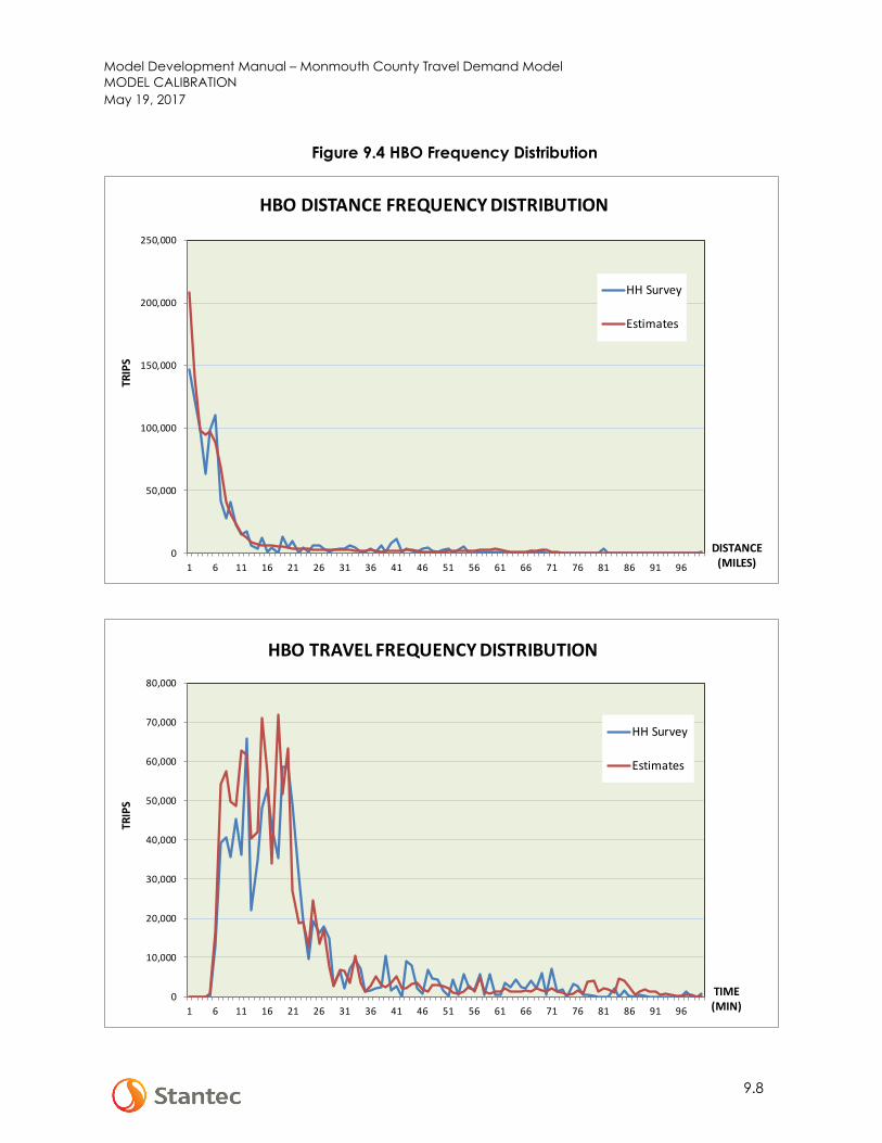
Model Development Manual – Monmouth County Travel Demand Model MODEL CALIBRATION May 19, 2017
9.8
Figure 9.4 HBO Frequency Distribution
0
50,000
100,000
150,000
200,000
250,000
1 6 11 16 21 26 31 36 41 46 51 56 61 66 71 76 81 86 91 96
TRIP
S
DISTANCE(MILES)
HBO DISTANCE FREQUENCY DISTRIBUTION
HH Survey
Estimates
0
10,000
20,000
30,000
40,000
50,000
60,000
70,000
80,000
1 6 11 16 21 26 31 36 41 46 51 56 61 66 71 76 81 86 91 96
TRIP
S
TIME(MIN)
HBO TRAVEL FREQUENCY DISTRIBUTION
HH Survey
Estimates

Model Development Manual – Monmouth County Travel Demand Model MODEL CALIBRATION May 19, 2017
9.9
Figure 9.5 NHBW Frequency Distribution
0
2,000
4,000
6,000
8,000
10,000
12,000
14,000
16,000
18,000
20,000
1 6 11 16 21 26 31 36 41 46 51 56 61 66 71 76 81 86 91 96
TRIP
S
DISTANCE(MILES)
NHBW DISTANCE FREQUENCY DISTRIBUTION
HH Survey
Estimates
0
2,000
4,000
6,000
8,000
10,000
12,000
1 6 11 16 21 26 31 36 41 46 51 56
TRIP
S
TIME(MIN)
NHBW TRAVEL TIME FREQUENCY DISTRIBUTION
HH Survey
Estimates

Model Development Manual – Monmouth County Travel Demand Model MODEL CALIBRATION May 19, 2017
9.10
Figure 9.6 NHBO Frequency Distribution
0
20,000
40,000
60,000
80,000
100,000
120,000
140,000
1 6 11 16 21 26 31 36 41 46 51 56 61 66 71 76 81 86 91 96
TRIP
S
DISTANCE(MILES)
NHBO DISTANCE FREQUENCY DISTRIBUTION
HH Survey
Estimates
0
10,000
20,000
30,000
40,000
50,000
60,000
1 6 11 16 21 26 31 36 41 46 51 56 61 66 71 76 81 86 91 96
TRIP
S
TIME(MIN)
NHBO TRAVEL TIME FREQUENCY DISTRIBUTION
HH Survey
Estimates

Model Development Manual – Monmouth County Travel Demand Model MODEL CALIBRATION May 19, 2017
9.11
Table 9.9 Trip Average Travel Time and Distance
Trip patterns can also be measured by district-to-district trip flows. District-to-district trip flows would help to gauge how close the estimated trip distribution replicated the observed data. In the MCTDM, a district is defined as a group of municipalities. Monmouth County is divided into 17 districts as shown in Table 9.10 and Figure 9.7. Outside Monmouth County, the region is divided into six external districts as shown in Table 9.11 and Figure 9.8. Prior to comparing the district-to-district trip flows, the percent shares of trip productions and trip attractions by trip purpose were compared first to measure the distribution of trip production and attraction across the district. Figures 9.9 to 9.13 show the percent distribution by district for each trip purpose. The estimated distribution by district replicated the observed data reasonably well.
OBSERVED ESTIMATED %DIFF OBSERVED ESTIMATED %DIFF OBSERVED ESTIMATED %DIFFHBW 30.1 28.5 -5.3% 55.8 53.8 -3.5% 32.3 31.7 -1.9%HBS 7.4 7.2 -1.7% 19.7 19.1 -3.2% 22.4 22.7 1.6%HBO 9.8 9.2 -6.3% 22.5 21.2 -5.9% 26.2 26.1 -0.4%NHBW 11.5 11.1 -3.5% 23.8 24.3 1.9% 28.8 27.3 -5.3%NHNW 9.6 9.2 -4.3% 22.0 21.1 -4.0% 26.2 26.2 -0.3%
TRIP PURPOSE
AVERAGE DISTANCE (MILES)
AVERAGE TRAVEL TIME(MINUTES)
AVERAGE SPEED(MPH)
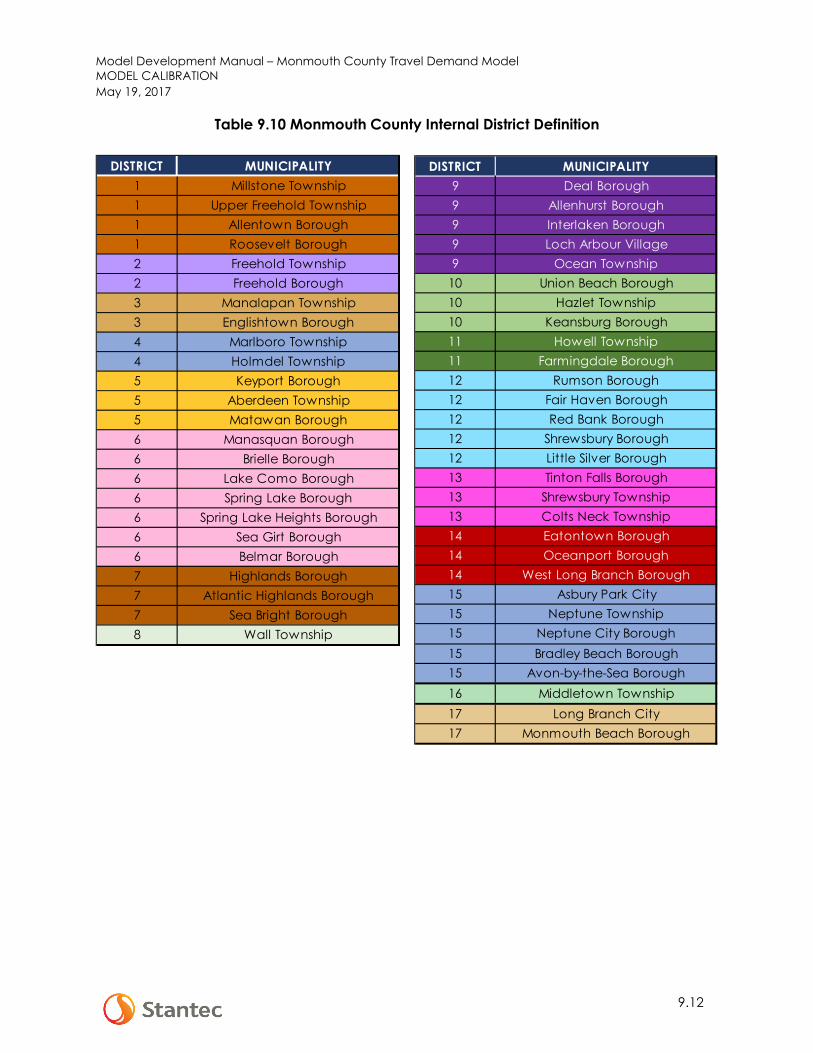
Model Development Manual – Monmouth County Travel Demand Model MODEL CALIBRATION May 19, 2017
9.12
Table 9.10 Monmouth County Internal District Definition
DISTRICT MUNICIPALITY1 Millstone Township1 Upper Freehold Township1 Allentown Borough1 Roosevelt Borough2 Freehold Township2 Freehold Borough3 Manalapan Township3 Englishtown Borough4 Marlboro Township4 Holmdel Township5 Keyport Borough5 Aberdeen Township5 Matawan Borough6 Manasquan Borough6 Brielle Borough6 Lake Como Borough6 Spring Lake Borough6 Spring Lake Heights Borough6 Sea Girt Borough6 Belmar Borough7 Highlands Borough7 Atlantic Highlands Borough7 Sea Bright Borough8 Wall Township
DISTRICT MUNICIPALITY9 Deal Borough9 Allenhurst Borough9 Interlaken Borough9 Loch Arbour Village9 Ocean Township
10 Union Beach Borough10 Hazlet Township10 Keansburg Borough11 Howell Township11 Farmingdale Borough12 Rumson Borough12 Fair Haven Borough12 Red Bank Borough12 Shrewsbury Borough12 Little Silver Borough13 Tinton Falls Borough13 Shrewsbury Township13 Colts Neck Township14 Eatontown Borough14 Oceanport Borough14 West Long Branch Borough15 Asbury Park City15 Neptune Township15 Neptune City Borough15 Bradley Beach Borough15 Avon-by-the-Sea Borough16 Middletown Township17 Long Branch City17 Monmouth Beach Borough
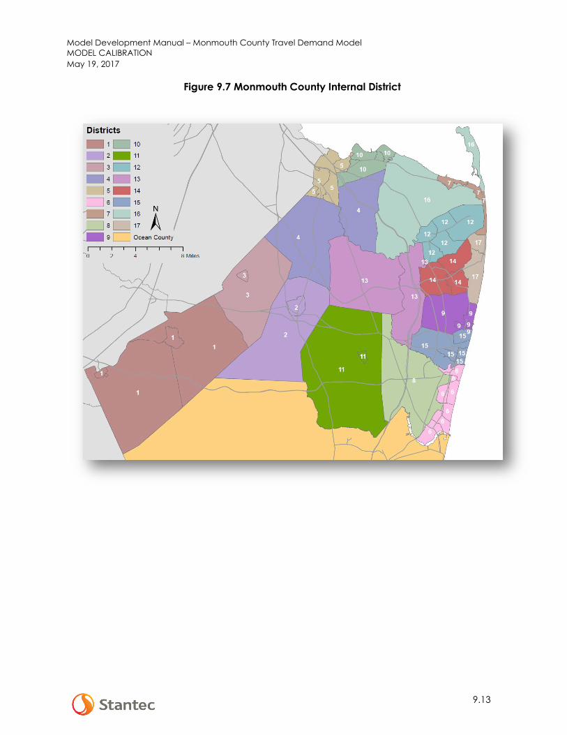
Model Development Manual – Monmouth County Travel Demand Model MODEL CALIBRATION May 19, 2017
9.13
Figure 9.7 Monmouth County Internal District

Model Development Manual – Monmouth County Travel Demand Model MODEL CALIBRATION May 19, 2017
9.14
Table 9.11 Monmouth County External District Definition
Figure 9.8 External District Definition
EXTERNAL DISTRICT DEFINITION
1 New York Five Boroughs and Long Island2 Northern and Central NJ (excluding the ones below) and NY3 Mercer/Burlington and PA4 Ocean/Atlantic and South Jersey5 Essex/Hudson6 Middlesex

Model Development Manual – Monmouth County Travel Demand Model MODEL CALIBRATION May 19, 2017
9.15
Figure 9.9 HBW Distribution by District
0.0%
5.0%
10.0%
15.0%
20.0%
25.0%
1 2 3 4 5 6 7 8 9 10 11 12 13 14 15 16 17
PERC
ENT
DIST
RIBU
TIO
N
DISTRICT NO.
PERCENT DISTRIBUTION PRODUCTION - HBW TOTAL
HH SURVEY LEHD-2014 ESTIMATED
0.0%
2.0%
4.0%
6.0%
8.0%
10.0%
12.0%
14.0%
1 2 3 4 5 6 7 8 9 10 11 12 13 14 15 16 17
PERC
ENT
DIST
RIBU
TIO
N
DISTRICT NO.
PERCENT DISTRIBUTION ATTRACTION - HBW TOTAL
HH SURVEY LEHD-2014 ESTIMATED

Model Development Manual – Monmouth County Travel Demand Model MODEL CALIBRATION May 19, 2017
9.16
Figure 9.10 HBS Distribution by District
0%
5%
10%
15%
20%
25%
1 2 3 4 5 6 7 8 9 10 11 12 13 14 15 16 17
PERC
ENT
DIST
RIBU
TIO
N
DISTRICT NO.
PERCENT DISTRIBUTION PRODUCTION - HBS
HH SURVEY ESTIMATED
0%
2%
4%
6%
8%
10%
12%
14%
16%
18%
20%
1 2 3 4 5 6 7 8 9 10 11 12 13 14 15 16 17
PERC
ENT
DIST
RIBU
TIO
N
DISTRICT NO.
PERCENT DISTRIBUTION ATTRACTION - HBS
HH SURVEY ESTIMATED

Model Development Manual – Monmouth County Travel Demand Model MODEL CALIBRATION May 19, 2017
9.17
Figure 9.11 HBO Distribution by District
0%
2%
4%
6%
8%
10%
12%
14%
16%
18%
20%
1 2 3 4 5 6 7 8 9 10 11 12 13 14 15 16 17
PERC
ENT
DIST
RIBU
TIO
N
DISTRICT NO.
PERCENT DISTRIBUTION PRODUCTION - HBO
HH SURVEY ESTIMATED
0%
2%
4%
6%
8%
10%
12%
14%
16%
18%
1 2 3 4 5 6 7 8 9 10 11 12 13 14 15 16 17
PERC
ENT
DIST
RIBU
TIO
N
DISTRICT NO.
PERCENT DISTRIBUTION ATTRACTION - HBO
HH SURVEY ESTIMATED

Model Development Manual – Monmouth County Travel Demand Model MODEL CALIBRATION May 19, 2017
9.18
Figure 9.12 NHBW Distribution by District
0%
2%
4%
6%
8%
10%
12%
14%
1 2 3 4 5 6 7 8 9 10 11 12 13 14 15 16 17
PERC
ENT
DIST
RIBU
TIO
N
DISTRICT NO.
PERCENT DISTRIBUTION PRODUCTION - NHBW
HH SURVEY ESTIMATED
0%
2%
4%
6%
8%
10%
12%
14%
1 2 3 4 5 6 7 8 9 10 11 12 13 14 15 16 17
PERC
ENT
DIST
RIBU
TIO
N
DISTRICT NO.
PERCENT DISTRIBUTION ATTRACTION - NHBW
HH SURVEY ESTIMATED

Model Development Manual – Monmouth County Travel Demand Model MODEL CALIBRATION May 19, 2017
9.19
Figure 9.13 NHBO Distribution by District
0%
2%
4%
6%
8%
10%
12%
14%
16%
18%
1 2 3 4 5 6 7 8 9 10 11 12 13 14 15 16 17
PERC
ENT
DIST
RIBU
TIO
N
DISTRICT NO.
PERCENT DISTRIBUTION PRODUCTION - NHBO
HH SURVEY ESTIMATED
0%
2%
4%
6%
8%
10%
12%
14%
16%
18%
1 2 3 4 5 6 7 8 9 10 11 12 13 14 15 16 17
PERC
ENT
DIST
RIBU
TIO
N
DISTRICT NO.
PERCENT DISTRIBUTION ATTRACTION - NHBO
HH SURVEY ESTIMATED

Model Development Manual – Monmouth County Travel Demand Model MODEL CALIBRATION May 19, 2017
9.20
The district-to-district trip flows for HBW are shown in Table 9.12. Considering that the household survey data at county level is very limited, LEHD data was used as the observed targets for the HBW purpose. The percentage of district-to-district trip flows were used in the calibration process, instead of using the trip values.
For other trip purposes, more aggregated district definitions are used due to limited observed data. The non-HBW district definition is shown in Table 9.13 and Figure 9.14. Tables 9.14 to 9.17 show district-to-district trip flow comparisons for non-HBW trip purposes. As expected, there are more variations between observed and estimated values at this level of comparison, although they are still within reasonable tolerance considering the limited observed data available.

Model Development Manual – Monmouth County Travel Demand Model MODEL CALIBRATION May 19, 2017
9.21
Table 9.12 Trip Flows Distribution by District - HBW
DISTRICT 1 2 3 4 5 6 7 8 9 10 11 12 13 14 15 16 17 18 19 20 21 22 23 TOTAL11.0% 5.7% 1.8% 1.7% 0.4% 0.3% 0.1% 1.1% 0.3% 0.3% 1.1% 1.0% 0.9% 0.9% 0.9% 0.9% 0.2% 0.0% 15.0% 23.5% 7.3% 6.8% 18.9% 100.0%18.6% 2.3% 0.6% 0.4% 0.2% 0.2% 0.1% 0.4% 0.2% 0.2% 0.6% 0.6% 0.4% 0.8% 0.5% 0.4% 0.4% 2.8% 15.6% 22.4% 10.0% 6.7% 15.7% 100.0%0.6% 19.3% 3.4% 3.8% 1.0% 0.4% 0.1% 1.7% 0.9% 0.7% 2.9% 2.2% 2.3% 2.1% 2.0% 2.0% 0.5% 0.0% 14.9% 9.1% 7.4% 6.3% 16.3% 100.0%0.3% 37.3% 1.9% 1.0% 0.3% 0.2% 0.1% 0.6% 0.3% 0.2% 4.7% 0.7% 1.1% 1.2% 0.8% 0.4% 0.6% 4.3% 13.8% 3.7% 9.7% 7.5% 9.3% 100.0%0.6% 8.9% 9.3% 6.7% 1.2% 0.4% 0.1% 1.1% 0.9% 0.8% 1.7% 1.5% 1.6% 1.4% 1.2% 1.9% 0.4% 0.0% 15.8% 9.7% 5.5% 6.5% 22.8% 100.0%0.5% 15.0% 14.7% 2.0% 0.3% 0.1% 0.1% 0.4% 0.2% 0.2% 1.7% 0.6% 0.5% 0.8% 0.4% 0.4% 0.4% 4.1% 16.0% 9.9% 6.1% 9.7% 15.9% 100.0%0.3% 4.7% 2.6% 11.8% 2.3% 0.3% 0.2% 1.1% 0.8% 2.0% 1.0% 2.7% 1.9% 1.9% 1.5% 4.5% 0.7% 0.0% 19.9% 4.9% 4.1% 9.3% 21.5% 100.0%0.1% 6.6% 3.4% 19.7% 2.0% 0.1% 0.1% 0.5% 0.2% 1.2% 1.1% 2.3% 1.6% 1.8% 0.4% 2.3% 0.4% 4.8% 18.1% 3.4% 3.7% 10.3% 16.0% 100.0%0.2% 2.9% 1.0% 4.9% 10.1% 0.1% 0.4% 1.2% 0.7% 4.4% 0.8% 3.3% 1.8% 2.3% 1.5% 3.5% 0.7% 0.0% 18.6% 3.9% 3.8% 8.4% 25.2% 100.0%0.1% 0.8% 0.3% 7.9% 16.5% 0.1% 0.2% 0.4% 0.3% 3.8% 0.4% 2.3% 1.0% 1.2% 0.5% 2.7% 0.6% 9.6% 17.7% 2.2% 4.0% 10.2% 17.2% 100.0%0.3% 3.5% 0.7% 1.6% 0.6% 16.5% 0.3% 8.7% 1.8% 0.6% 2.0% 3.0% 2.6% 2.8% 6.8% 2.2% 1.0% 0.0% 12.3% 5.3% 13.8% 5.9% 7.9% 100.0%0.1% 0.7% 0.2% 0.3% 0.2% 14.9% 0.1% 15.0% 1.4% 0.1% 1.0% 0.8% 0.7% 2.1% 7.2% 0.3% 1.5% 4.1% 9.7% 3.3% 22.4% 5.8% 8.2% 100.0%0.2% 2.5% 0.5% 2.6% 1.4% 0.5% 11.9% 1.6% 1.6% 2.6% 0.9% 10.5% 2.7% 4.1% 2.5% 9.3% 2.1% 0.0% 16.0% 3.8% 3.7% 8.2% 10.9% 100.0%0.1% 0.4% 0.1% 1.0% 0.6% 0.2% 9.6% 0.3% 0.7% 0.8% 0.2% 9.9% 0.7% 8.1% 0.7% 4.7% 13.5% 10.2% 14.2% 1.8% 3.8% 9.6% 8.8% 100.0%0.2% 3.2% 0.6% 1.5% 0.5% 8.5% 0.2% 13.8% 2.2% 0.6% 2.1% 3.2% 2.7% 3.4% 10.6% 2.1% 1.1% 0.0% 11.9% 4.8% 13.7% 5.7% 7.5% 100.0%0.1% 0.9% 0.2% 0.4% 0.2% 4.4% 0.1% 28.8% 1.2% 0.1% 1.9% 0.8% 1.1% 2.1% 5.9% 0.3% 0.9% 5.0% 10.4% 3.2% 18.4% 5.5% 8.2% 100.0%0.1% 3.7% 0.7% 2.1% 0.9% 1.4% 0.4% 3.3% 14.1% 0.8% 1.3% 5.9% 5.2% 8.8% 9.5% 3.1% 4.5% 0.0% 11.6% 4.0% 5.7% 5.7% 7.3% 100.0%0.1% 0.6% 0.1% 0.4% 0.2% 0.6% 0.1% 1.7% 19.5% 0.1% 0.5% 3.1% 2.8% 18.4% 10.0% 0.6% 4.7% 5.9% 10.8% 2.2% 4.7% 6.0% 6.5% 100.0%0.1% 3.1% 0.7% 5.6% 3.8% 0.2% 0.7% 1.4% 1.0% 13.2% 0.8% 4.0% 2.0% 2.2% 1.8% 6.2% 0.8% 0.0% 17.4% 4.2% 3.6% 9.0% 17.9% 100.0%0.1% 0.6% 0.2% 5.9% 4.2% 0.1% 0.7% 0.4% 0.3% 12.4% 0.3% 5.7% 0.8% 2.1% 0.6% 6.6% 1.0% 12.3% 16.5% 1.9% 4.2% 9.5% 13.6% 100.0%0.4% 8.9% 1.6% 2.4% 0.7% 1.3% 0.2% 4.1% 1.6% 0.6% 10.2% 2.4% 2.7% 2.8% 3.1% 1.8% 0.9% 0.0% 12.6% 7.4% 15.7% 5.5% 13.1% 100.0%0.2% 7.2% 0.4% 0.5% 0.2% 0.4% 0.1% 1.6% 0.3% 0.1% 20.4% 0.6% 0.8% 0.9% 1.1% 0.3% 0.5% 3.1% 11.9% 3.7% 30.5% 6.4% 8.9% 100.0%0.2% 2.3% 0.4% 2.5% 1.4% 0.4% 1.3% 1.8% 2.0% 1.2% 0.9% 24.2% 4.8% 4.9% 3.3% 6.4% 2.6% 0.0% 14.7% 3.7% 3.9% 7.7% 9.5% 100.0%0.1% 0.3% 0.1% 0.6% 0.3% 0.1% 0.5% 0.3% 0.9% 0.3% 0.2% 39.5% 2.4% 11.2% 0.6% 3.1% 4.1% 5.3% 11.8% 2.0% 2.8% 7.1% 6.5% 100.0%0.2% 4.2% 0.9% 3.5% 1.3% 0.7% 0.5% 2.5% 2.9% 1.1% 1.8% 9.0% 10.9% 5.8% 4.8% 4.9% 2.1% 0.0% 14.5% 4.9% 6.6% 7.3% 9.7% 100.0%0.1% 2.0% 0.3% 2.0% 0.4% 0.3% 0.1% 2.2% 1.7% 0.2% 1.6% 5.9% 18.8% 10.7% 3.1% 1.7% 1.9% 6.8% 14.2% 2.6% 5.2% 8.7% 9.4% 100.0%0.1% 3.4% 0.6% 2.0% 0.9% 0.6% 0.8% 2.6% 4.6% 1.0% 1.1% 9.7% 5.7% 15.5% 4.4% 3.5% 7.6% 0.0% 12.3% 4.0% 5.5% 6.1% 8.0% 100.0%0.1% 0.5% 0.1% 0.5% 0.2% 0.3% 0.3% 0.6% 3.3% 0.2% 0.3% 6.5% 2.6% 35.3% 2.3% 1.0% 11.0% 5.4% 11.1% 2.0% 3.9% 6.5% 6.1% 100.0%0.2% 3.9% 0.8% 1.7% 0.6% 1.8% 0.2% 4.9% 4.1% 0.7% 1.7% 4.3% 5.6% 5.5% 21.6% 2.0% 2.2% 0.0% 11.2% 4.7% 9.8% 5.5% 7.1% 100.0%0.1% 0.8% 0.2% 0.5% 0.3% 2.3% 0.1% 4.8% 5.0% 0.2% 0.8% 1.9% 2.3% 5.9% 30.1% 0.5% 3.7% 5.3% 10.6% 2.5% 7.8% 6.0% 8.2% 100.0%0.1% 2.6% 0.7% 4.0% 1.9% 0.4% 2.0% 1.8% 1.3% 3.4% 1.0% 10.3% 3.6% 3.3% 2.7% 16.9% 1.2% 0.0% 14.8% 3.8% 3.8% 8.0% 12.3% 100.0%0.1% 0.4% 0.1% 1.9% 0.9% 0.1% 1.2% 0.3% 0.4% 1.7% 0.2% 17.3% 2.1% 4.7% 0.5% 20.8% 2.0% 6.6% 15.0% 2.0% 3.4% 8.7% 9.4% 100.0%0.1% 2.7% 0.4% 1.6% 0.7% 0.8% 0.6% 2.3% 3.7% 1.0% 1.1% 7.6% 3.7% 9.9% 5.2% 2.4% 16.3% 0.0% 14.2% 4.3% 5.9% 7.1% 8.5% 100.0%0.1% 0.5% 0.2% 0.4% 0.2% 0.4% 0.6% 0.6% 2.5% 0.2% 0.3% 4.7% 1.4% 18.8% 2.5% 0.8% 28.0% 6.6% 11.0% 2.1% 4.4% 6.6% 7.1% 100.0%1.1% 9.1% 5.5% 13.0% 5.4% 2.4% 2.1% 4.3% 4.8% 4.8% 4.5% 10.1% 5.1% 7.9% 5.0% 11.6% 3.3% 100.0%1.1% 9.7% 3.0% 9.3% 6.7% 1.6% 1.3% 4.5% 3.1% 5.0% 3.8% 11.9% 5.3% 11.6% 6.4% 8.4% 7.3% 100.0%1.3% 12.5% 5.1% 8.6% 4.5% 1.7% 0.6% 6.3% 3.6% 5.0% 5.9% 8.3% 6.2% 10.4% 5.8% 12.4% 1.8% 100.0%2.1% 10.3% 3.5% 8.5% 5.3% 2.1% 1.4% 5.2% 3.0% 3.7% 4.7% 12.4% 5.8% 11.1% 6.3% 7.9% 6.9% 100.0%11.2% 16.8% 6.7% 7.2% 2.3% 1.6% 0.4% 6.0% 2.9% 2.6% 8.8% 6.4% 6.5% 7.8% 4.5% 7.0% 1.3% 100.0%7.0% 15.0% 3.2% 5.9% 2.8% 3.2% 0.7% 7.7% 3.6% 1.9% 7.9% 8.6% 5.0% 8.9% 8.8% 4.9% 4.9% 100.0%2.5% 12.8% 3.0% 4.5% 1.5% 5.7% 0.4% 13.9% 4.7% 1.3% 11.8% 6.1% 6.4% 7.4% 11.5% 3.9% 2.5% 100.0%3.1% 12.6% 2.8% 4.5% 2.4% 5.6% 0.7% 11.9% 3.7% 1.4% 11.8% 7.1% 4.8% 9.1% 9.3% 3.6% 5.7% 100.0%1.3% 12.1% 4.0% 8.7% 5.4% 1.5% 0.6% 5.7% 2.5% 4.8% 6.1% 9.0% 7.1% 13.0% 5.4% 10.0% 2.7% 100.0%1.3% 10.1% 3.2% 7.5% 4.9% 2.1% 1.4% 5.4% 3.3% 3.4% 4.3% 12.0% 6.2% 13.2% 6.8% 7.1% 7.8% 100.0%1.8% 14.4% 8.1% 15.0% 8.2% 0.9% 0.5% 3.9% 2.2% 6.4% 4.7% 7.2% 5.8% 6.8% 4.4% 8.7% 1.1% 100.0%1.9% 12.0% 6.9% 9.6% 8.2% 2.0% 1.2% 4.8% 2.8% 3.3% 4.6% 9.6% 4.9% 9.9% 6.2% 5.8% 6.3% 100.0%
TOTALATTRACTION
NOTE:1234% Observed Data from LEHD data1234% Model Estimated
7
8
9
1
2
3
4
5
20
21
22
23
15
16
17
18
19
10
11
12
13
14
6

Model Development Manual – Monmouth County Travel Demand Model MODEL CALIBRATION May 19, 2017
9.22
This Page is Intentionally Left Blank
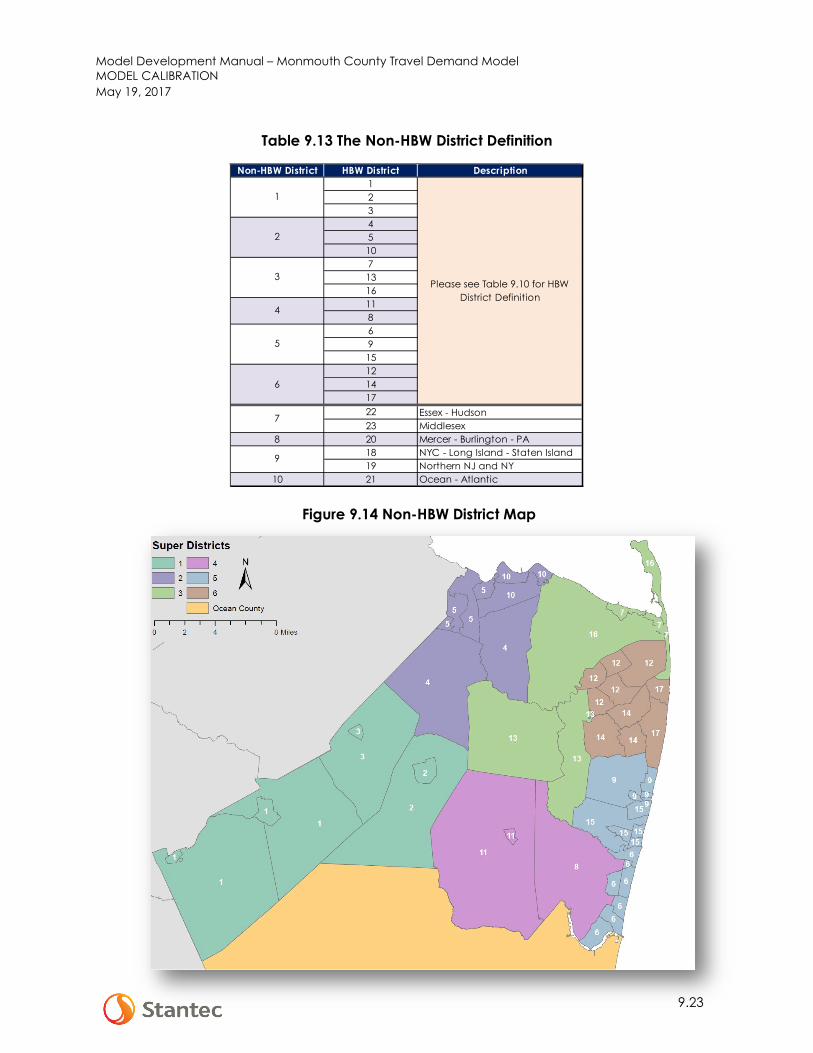
Model Development Manual – Monmouth County Travel Demand Model MODEL CALIBRATION May 19, 2017
9.23
Table 9.13 The Non-HBW District Definition
Figure 9.14 Non-HBW District Map
Non-HBW District HBW District Description123451071316118691512141722 Essex - Hudson23 Middlesex
8 20 Mercer - Burlington - PA18 NYC - Long Island - Staten Island19 Northern NJ and NY
10 21 Ocean - Atlantic
Please see Table 9.10 for HBW District Definition
7
9
1
2
3
4
5
6
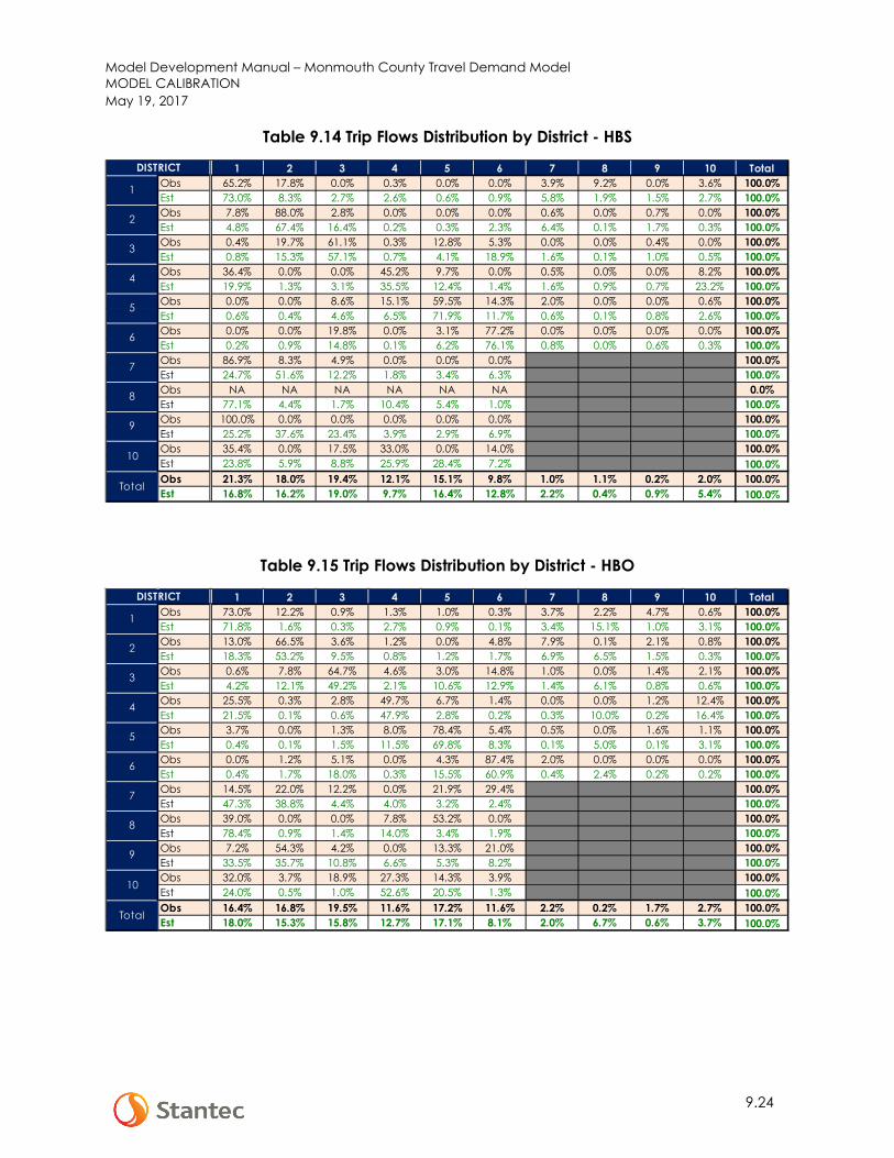
Model Development Manual – Monmouth County Travel Demand Model MODEL CALIBRATION May 19, 2017
9.24
Table 9.14 Trip Flows Distribution by District - HBS
Table 9.15 Trip Flows Distribution by District - HBO
1 2 3 4 5 6 7 8 9 10 TotalObs 65.2% 17.8% 0.0% 0.3% 0.0% 0.0% 3.9% 9.2% 0.0% 3.6% 100.0%Est 73.0% 8.3% 2.7% 2.6% 0.6% 0.9% 5.8% 1.9% 1.5% 2.7% 100.0%Obs 7.8% 88.0% 2.8% 0.0% 0.0% 0.0% 0.6% 0.0% 0.7% 0.0% 100.0%Est 4.8% 67.4% 16.4% 0.2% 0.3% 2.3% 6.4% 0.1% 1.7% 0.3% 100.0%Obs 0.4% 19.7% 61.1% 0.3% 12.8% 5.3% 0.0% 0.0% 0.4% 0.0% 100.0%Est 0.8% 15.3% 57.1% 0.7% 4.1% 18.9% 1.6% 0.1% 1.0% 0.5% 100.0%Obs 36.4% 0.0% 0.0% 45.2% 9.7% 0.0% 0.5% 0.0% 0.0% 8.2% 100.0%Est 19.9% 1.3% 3.1% 35.5% 12.4% 1.4% 1.6% 0.9% 0.7% 23.2% 100.0%Obs 0.0% 0.0% 8.6% 15.1% 59.5% 14.3% 2.0% 0.0% 0.0% 0.6% 100.0%Est 0.6% 0.4% 4.6% 6.5% 71.9% 11.7% 0.6% 0.1% 0.8% 2.6% 100.0%Obs 0.0% 0.0% 19.8% 0.0% 3.1% 77.2% 0.0% 0.0% 0.0% 0.0% 100.0%Est 0.2% 0.9% 14.8% 0.1% 6.2% 76.1% 0.8% 0.0% 0.6% 0.3% 100.0%Obs 86.9% 8.3% 4.9% 0.0% 0.0% 0.0% 100.0%Est 24.7% 51.6% 12.2% 1.8% 3.4% 6.3% 100.0%Obs NA NA NA NA NA NA 0.0%Est 77.1% 4.4% 1.7% 10.4% 5.4% 1.0% 100.0%Obs 100.0% 0.0% 0.0% 0.0% 0.0% 0.0% 100.0%Est 25.2% 37.6% 23.4% 3.9% 2.9% 6.9% 100.0%Obs 35.4% 0.0% 17.5% 33.0% 0.0% 14.0% 100.0%Est 23.8% 5.9% 8.8% 25.9% 28.4% 7.2% 100.0%Obs 21.3% 18.0% 19.4% 12.1% 15.1% 9.8% 1.0% 1.1% 0.2% 2.0% 100.0%Est 16.8% 16.2% 19.0% 9.7% 16.4% 12.8% 2.2% 0.4% 0.9% 5.4% 100.0%
Total
DISTRICT
1
2
3
4
5
6
7
8
9
10
1 2 3 4 5 6 7 8 9 10 TotalObs 73.0% 12.2% 0.9% 1.3% 1.0% 0.3% 3.7% 2.2% 4.7% 0.6% 100.0%Est 71.8% 1.6% 0.3% 2.7% 0.9% 0.1% 3.4% 15.1% 1.0% 3.1% 100.0%Obs 13.0% 66.5% 3.6% 1.2% 0.0% 4.8% 7.9% 0.1% 2.1% 0.8% 100.0%Est 18.3% 53.2% 9.5% 0.8% 1.2% 1.7% 6.9% 6.5% 1.5% 0.3% 100.0%Obs 0.6% 7.8% 64.7% 4.6% 3.0% 14.8% 1.0% 0.0% 1.4% 2.1% 100.0%Est 4.2% 12.1% 49.2% 2.1% 10.6% 12.9% 1.4% 6.1% 0.8% 0.6% 100.0%Obs 25.5% 0.3% 2.8% 49.7% 6.7% 1.4% 0.0% 0.0% 1.2% 12.4% 100.0%Est 21.5% 0.1% 0.6% 47.9% 2.8% 0.2% 0.3% 10.0% 0.2% 16.4% 100.0%Obs 3.7% 0.0% 1.3% 8.0% 78.4% 5.4% 0.5% 0.0% 1.6% 1.1% 100.0%Est 0.4% 0.1% 1.5% 11.5% 69.8% 8.3% 0.1% 5.0% 0.1% 3.1% 100.0%Obs 0.0% 1.2% 5.1% 0.0% 4.3% 87.4% 2.0% 0.0% 0.0% 0.0% 100.0%Est 0.4% 1.7% 18.0% 0.3% 15.5% 60.9% 0.4% 2.4% 0.2% 0.2% 100.0%Obs 14.5% 22.0% 12.2% 0.0% 21.9% 29.4% 100.0%Est 47.3% 38.8% 4.4% 4.0% 3.2% 2.4% 100.0%Obs 39.0% 0.0% 0.0% 7.8% 53.2% 0.0% 100.0%Est 78.4% 0.9% 1.4% 14.0% 3.4% 1.9% 100.0%Obs 7.2% 54.3% 4.2% 0.0% 13.3% 21.0% 100.0%Est 33.5% 35.7% 10.8% 6.6% 5.3% 8.2% 100.0%Obs 32.0% 3.7% 18.9% 27.3% 14.3% 3.9% 100.0%Est 24.0% 0.5% 1.0% 52.6% 20.5% 1.3% 100.0%Obs 16.4% 16.8% 19.5% 11.6% 17.2% 11.6% 2.2% 0.2% 1.7% 2.7% 100.0%Est 18.0% 15.3% 15.8% 12.7% 17.1% 8.1% 2.0% 6.7% 0.6% 3.7% 100.0%
Total
DISTRICT
1
2
3
4
5
6
7
8
9
10

Model Development Manual – Monmouth County Travel Demand Model MODEL CALIBRATION May 19, 2017
9.25
Table 9.16 Trip Flows Distribution by District - NHBW
Table 9.17 Trip Flows Distribution by District - NHBO
1 2 3 4 5 6 7 8 9 10 TotalObs 77.8% 5.9% 1.0% 8.3% 0.0% 0.8% 1.7% 0.6% 0.6% 3.2% 100.0%Est 52.1% 6.1% 4.1% 8.0% 2.7% 2.8% 12.0% 2.7% 2.0% 7.4% 100.0%Obs 10.6% 63.3% 17.3% 0.0% 0.0% 2.7% 1.6% 0.0% 3.8% 0.7% 100.0%Est 9.9% 36.3% 14.6% 2.6% 2.4% 7.9% 18.7% 0.1% 6.1% 1.5% 100.0%Obs 1.5% 13.8% 45.4% 1.5% 7.7% 23.4% 2.3% 0.3% 0.7% 3.5% 100.0%Est 6.1% 12.3% 36.1% 4.5% 7.1% 21.2% 6.8% 0.1% 2.4% 3.4% 100.0%Obs 13.3% 0.0% 1.7% 42.5% 22.0% 2.1% 2.0% 0.0% 1.4% 15.0% 100.0%Est 13.7% 2.7% 5.7% 32.4% 13.7% 5.1% 2.9% 0.9% 0.5% 22.4% 100.0%Obs 0.0% 0.0% 9.2% 23.3% 42.0% 17.9% 0.4% 0.0% 0.6% 6.6% 100.0%Est 4.7% 2.7% 9.1% 14.1% 41.0% 14.7% 2.0% 0.2% 0.5% 11.0% 100.0%Obs 0.9% 1.8% 19.9% 1.6% 12.7% 51.0% 0.2% 0.0% 0.6% 11.1% 100.0%Est 3.6% 5.7% 18.1% 3.5% 10.4% 52.1% 3.2% 0.0% 1.2% 2.4% 100.0%Obs 28.8% 14.9% 27.3% 21.7% 4.1% 3.3% 100.0%Est 37.4% 32.2% 14.0% 5.6% 3.4% 7.5% 100.0%Obs 76.7% 0.0% 23.3% 0.0% 0.0% 0.0% 100.0%Est 74.1% 2.3% 1.9% 17.6% 3.2% 0.8% 100.0%Obs 11.4% 42.8% 10.5% 17.1% 7.4% 10.8% 100.0%Est 25.5% 39.6% 18.7% 3.8% 2.6% 9.8% 100.0%Obs 11.4% 1.4% 8.5% 32.9% 13.6% 32.2% 100.0%Est 21.6% 2.8% 7.5% 41.7% 19.7% 6.7% 100.0%Obs 21.3% 11.9% 14.9% 13.3% 12.5% 17.6% 1.2% 0.2% 1.0% 6.1% 100.0%Est 19.7% 11.0% 13.7% 12.2% 11.6% 16.3% 6.5% 0.7% 1.7% 6.6% 100.0%
Total
DISTRICT
1
2
3
4
5
6
7
8
9
10
1 2 3 4 5 6 7 8 9 10 TotalObs 67.1% 3.9% 7.0% 5.0% 3.1% 0.2% 5.0% 2.8% 1.8% 4.0% 100.0%Est 72.3% 2.5% 2.0% 6.0% 1.1% 0.4% 7.4% 2.4% 3.0% 3.0% 100.0%Obs 6.1% 64.0% 14.2% 0.3% 0.6% 2.0% 8.1% 0.0% 3.0% 1.5% 100.0%Est 3.6% 53.2% 18.8% 0.4% 0.7% 1.8% 15.2% 0.4% 5.1% 0.6% 100.0%Obs 6.4% 8.3% 65.3% 1.5% 7.7% 9.3% 0.5% 0.0% 0.3% 0.6% 100.0%Est 1.8% 11.3% 58.4% 1.5% 6.5% 11.8% 3.4% 0.6% 3.8% 0.9% 100.0%Obs 11.9% 0.4% 3.8% 35.4% 17.5% 5.3% 0.4% 0.0% 4.6% 20.7% 100.0%Est 14.4% 0.7% 4.0% 38.9% 17.8% 1.1% 2.7% 1.1% 2.6% 16.6% 100.0%Obs 3.0% 0.4% 8.0% 7.1% 68.3% 6.5% 0.7% 0.0% 1.1% 5.0% 100.0%Est 1.0% 0.5% 7.0% 7.1% 68.5% 7.3% 1.5% 0.5% 2.0% 4.6% 100.0%Obs 0.4% 2.3% 18.2% 4.0% 12.0% 58.4% 1.2% 0.0% 1.5% 1.9% 100.0%Est 0.8% 2.1% 23.5% 0.8% 14.0% 53.3% 1.8% 0.5% 2.6% 0.6% 100.0%Obs 40.3% 41.8% 4.8% 1.4% 6.2% 5.5% 100.0%Est 31.2% 40.1% 14.1% 4.4% 6.1% 4.0% 100.0%Obs 100.0% 0.0% 0.0% 0.0% 0.0% 0.0% 100.0%Est 48.7% 7.8% 13.4% 9.6% 13.3% 7.2% 100.0%Obs 23.2% 24.0% 4.0% 24.1% 14.0% 10.7% 100.0%Est 21.5% 21.0% 27.8% 7.1% 13.1% 9.5% 100.0%Obs 19.6% 4.7% 3.4% 42.0% 25.1% 5.2% 100.0%Est 17.5% 2.6% 6.6% 42.4% 28.4% 2.5% 100.0%Obs 19.4% 12.2% 21.0% 8.1% 20.1% 10.8% 2.4% 0.5% 1.5% 4.0% 100.0%Est 18.8% 11.8% 20.2% 7.9% 19.6% 10.3% 4.6% 0.9% 2.8% 3.1% 100.0%
Total
DISTRICT
1
2
3
4
5
6
7
8
9
10

Model Development Manual – Monmouth County Travel Demand Model MODEL CALIBRATION May 19, 2017
9.26
9.4 MODE CHOICE
The mode choice model for the MCTDM is adopted from the NJRTM-E and the NJ Transit’s North Jersey Travel Demand Forecasting Model (NJTDFM). The model was developed using a C-Based programming language and invoked by the NJRTM-E within Cube Environment. This C-Based mode choice model replaces the older mode choice model developed using FORTRAN programming language. The mode choice is a typical step within a traditional 4-step travel forecasting model. In this step, trips in each TAZ-to-TAZ cell of the person trip table are divided among different available travel modes. The selection of travel mode is a function of the characteristics of each mode that is available for that particular origin-destination TAZ pair and the characteristics of the traveler, the production TAZ, and the attraction TAZ. The mathematical function used in the mode choice model to perform this split is known as a nested logit model. Figure 9.15 shows the nesting structure of this model.
The logit model is structured so that for each Production and Attraction TAZ pair, the percentage (or share) of trips choosing a given mode a from a choice of m modes is equal to the exponential of utility associated with mode a divided by the sum of the exponential of utility for all m modes. The equation is:
Pe
ea
U
U
i
m
a
i
=
=∑
1 where, Pa is the probability of a traveler choosing mode a; Ua is the utility (or attractiveness) of mode a; and ΣUi is the sum of the utilities for all m modes.
The utility equation, Ua, is mode-specific and can be represented in the following general form:
aaaaa CimeInVehicleTcFarecDistancecU ++×+×+×= 321 where, Ua is the utility (or attractiveness) of mode a; Distancea, Farea, and In-Vehicle Timea - are level of service variables of mode a for this trip c1,c2,.. are coefficients estimated for each of the terms based on survey results ca is the constant for mode a – obtained through calibration
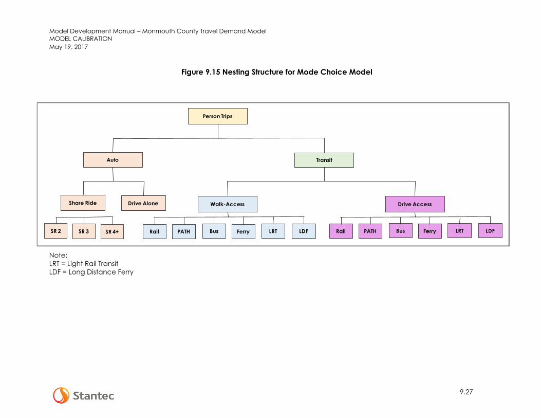
Model Development Manual – Monmouth County Travel Demand Model MODEL CALIBRATION May 19, 2017
9.27
Figure 9.15 Nesting Structure for Mode Choice Model
Note: LRT = Light Rail Transit LDF = Long Distance Ferry
Person Trips
Auto Transit
Share Ride Drive Alone
SR 2 SR 3 SR 4+
Walk-Access Drive Access
Rail PATH Bus Ferry LRT LDF Rail PATH Bus Ferry LRT LDF

Model Development Manual – Monmouth County Travel Demand Model MODEL CALIBRATION May 19, 2017
9.28
This Page is Intentionally Left Blank

Model Development Manual – Monmouth County Travel Demand Model MODEL CALIBRATION May 19, 2017
9.29
The models are structured as a series of choices, or also known as nests, such as transit vs. auto or walk access vs. drive access to transit. The nested logit structure implies that the share of trips choosing a particular mode b is dependent upon the logarithm of the sum (logsum) of the exponential of modal utilities of those sub-modes nesting below mode b. This is computed as:
U c e Cb nestU
i
n
bi= ×
+
=∑ln
1 where: Ub is the utility for nest b Cnest is a coefficient called the nesting coefficient, or theta; and Cb is a nest level constant for nest b– obtained through calibration.
The calibration was performed by adjusting these mode choice coefficients and comparing model estimated person trips by travel mode to the observed targets obtained from the Household Survey Data. The model consists of four major auto modes:
- Single Occupancy Vehicles (SOV) - High Occupancy Vehicle with 2 occupants (HOV2) - High Occupancy Vehicles with 3 occupants (HOV3) - High Occupancy Vehicles with 4 or more occupants (HOV4+)
And two transit sub-modes:
- Walk to transit - Drive to transit
Each transit sub-modes consists of commuter rail, bus, PATH, subway, light rail, and Ferry. The percent mode share comparison for each trip purpose is shown in Table 9.18 to Table 9.23. The model estimated percent mode shares replicated the observed data reasonably well.
Table 9.18 Mode Choice Comparison - HBWD
Pct PctSOV 77.4% 80.2%
HOV2 7.2% 6.6%HOV3 0.3% 0.4%HOV4 0.0% 0.3%
Walk-Transit 2.4% 3.6%Drive-Transit 12.8% 8.9%
TOTAL 100.0% 100.0%
2010 RHTS EstimatedMODEHBWD (Person Trips)

Model Development Manual – Monmouth County Travel Demand Model MODEL CALIBRATION May 19, 2017
9.30
Table 9.19 Mode Choice Comparison - HBWS
Table 9.20 Mode Choice Comparison - HBS
Table 9.21 Mode Choice Comparison - HBO
Pct PctSOV 85.4% 80.3%
HOV2 11.2% 13.6%HOV3 1.2% 3.7%HOV4 2.2% 2.3%
Walk-Transit 0.0% 0.1%Drive-Transit 0.0% 0.0%
TOTAL 100.0% 100.0%
HBWS (Person Trips)2010 RHTS EstimatedMODE
Pct PctSOV 57.5% 57.8%
HOV2 24.2% 27.7%HOV3 14.6% 10.2%HOV4 2.1% 3.7%
Walk-Transit 1.6% 0.5%Drive-Transit 0.0% 0.1%
TOTAL 100.0% 100.0%
MODEHBS (Person Trips)
2010 RHTS Estimated
Pct PctSOV 45.4% 46.9%
HOV2 28.0% 29.3%HOV3 16.6% 15.9%HOV4 8.5% 7.7%
Walk-Transit 0.8% 0.1%Drive-Transit 0.7% 0.1%
TOTAL 100.0% 100.0%
HBO (Person Trips)2010 RHTS EstimatedMODE

Model Development Manual – Monmouth County Travel Demand Model MODEL CALIBRATION May 19, 2017
9.31
Table 9.22 Mode Choice Comparison - NHBW
Table 9.23 Mode Choice Comparison - NHBO
9.5 HIGHWAY ASSIGNMENT
The highway assignment model was performed for four different time periods, AM Peak, PM Peak, Midday, and Night, as discussed in Section 9.1. In order to prepare these four-period highway assignments, the daily trip tables by purpose were stratified into four time-of-day trip tables using the factors developed from the Household Survey Data. The time-of-day factors are shown in Table 9.24. The factors for the home-based trip purposes were differentiated by the direction of travel (Production/Home to Attraction and Attraction to Production/Home), while the non-home based trip purposes assume the same factor for both directions.
Pct PctSOV 80.6% 80.5%
HOV2 18.0% 18.5%HOV3 0.5% 0.8%HOV4 0.8% 0.2%
Walk-Transit 0.0% 0.0%Drive-Transit 0.0% 0.0%
TOTAL 100.0% 100.0%
MODENHBW (Person Trips)
2010 RHTS Estimated
Pct PctSOV 44.7% 43.7%
HOV2 35.7% 37.3%HOV3 15.2% 15.5%HOV4 4.1% 3.4%
Walk-Transit 0.1% 0.1%Drive-Transit 0.1% 0.1%
TOTAL 100.0% 100.0%
NHBO (Person Trips)2010 RHTS EstimatedMODE
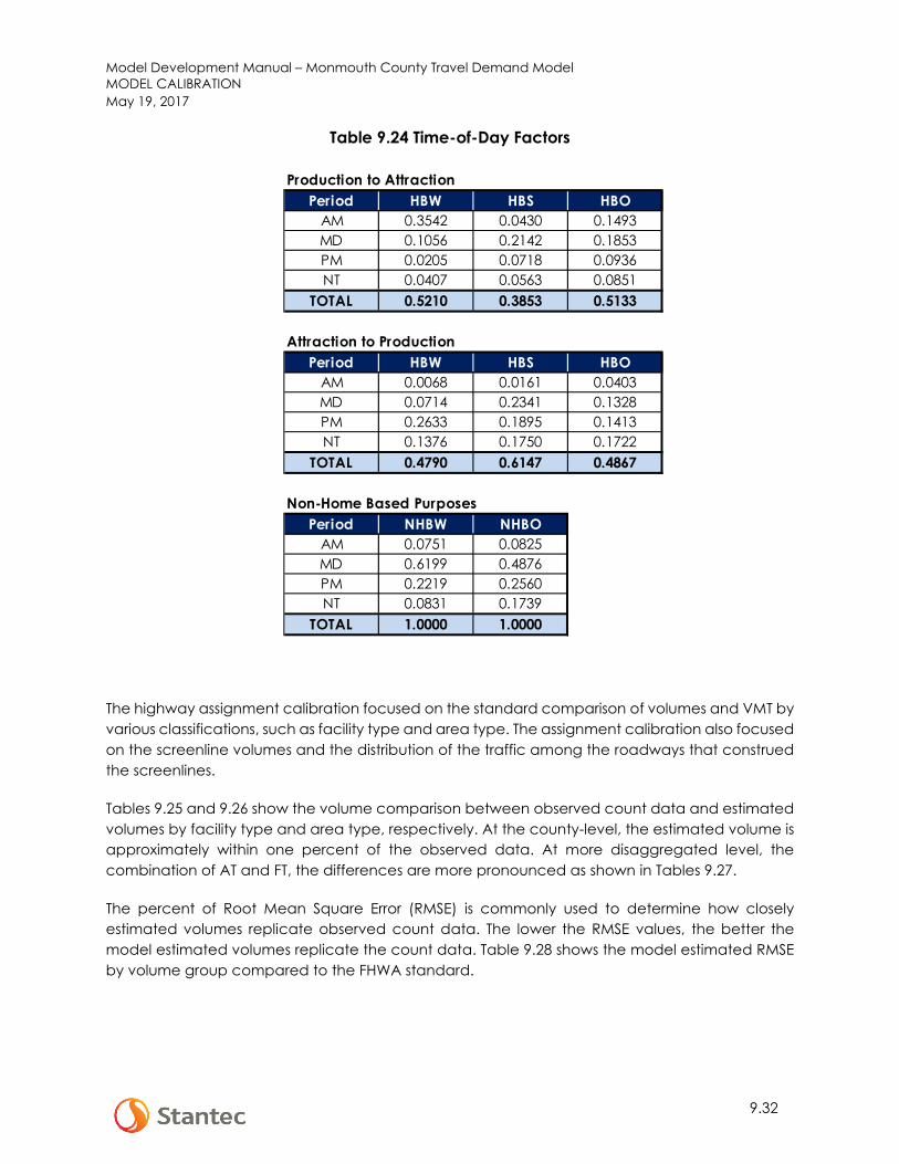
Model Development Manual – Monmouth County Travel Demand Model MODEL CALIBRATION May 19, 2017
9.32
Table 9.24 Time-of-Day Factors
The highway assignment calibration focused on the standard comparison of volumes and VMT by various classifications, such as facility type and area type. The assignment calibration also focused on the screenline volumes and the distribution of the traffic among the roadways that construed the screenlines.
Tables 9.25 and 9.26 show the volume comparison between observed count data and estimated volumes by facility type and area type, respectively. At the county-level, the estimated volume is approximately within one percent of the observed data. At more disaggregated level, the combination of AT and FT, the differences are more pronounced as shown in Tables 9.27.
The percent of Root Mean Square Error (RMSE) is commonly used to determine how closely estimated volumes replicate observed count data. The lower the RMSE values, the better the model estimated volumes replicate the count data. Table 9.28 shows the model estimated RMSE by volume group compared to the FHWA standard.
Production to AttractionPeriod HBW HBS HBO
AM 0.3542 0.0430 0.1493MD 0.1056 0.2142 0.1853PM 0.0205 0.0718 0.0936NT 0.0407 0.0563 0.0851
TOTAL 0.5210 0.3853 0.5133
Attraction to ProductionPeriod HBW HBS HBO
AM 0.0068 0.0161 0.0403MD 0.0714 0.2341 0.1328PM 0.2633 0.1895 0.1413NT 0.1376 0.1750 0.1722
TOTAL 0.4790 0.6147 0.4867
Non-Home Based PurposesPeriod NHBW NHBO
AM 0.0751 0.0825MD 0.6199 0.4876PM 0.2219 0.2560NT 0.0831 0.1739
TOTAL 1.0000 1.0000

Model Development Manual – Monmouth County Travel Demand Model MODEL CALIBRATION May 19, 2017
9.33
Table 9.25 Comparison by Facility Type
Table 9.26 Comparison by Area Type
OBSERVED ESTIMATED EST/OBSLimited-Access Facility 3,656,436 3,497,673 0.96Expressway 198,964 186,218 0.94Principal Arterial Divided 510,588 454,914 0.89Principal Arterial Undivided 466,781 483,220 1.04Minor Arterial Divided 294,106 260,664 0.89Minor Arterial Undivided 1,014,673 1,035,818 1.02Minor Arterials 1,835,628 1,967,082 1.07Collector/Local 63,316 101,551 1.60
TOTAL 8,040,492 7,987,140 0.99
FACILITY TYPEVOLUME
OBSERVED ESTIMATED EST/OBSUrban 505,432 538,131 1.06
Suburban 6,789,820 6,645,734 0.98Rural 745,240 803,275 1.08TOTAL 8,040,492 7,987,140 0.99
AREA TYPEVOLUME
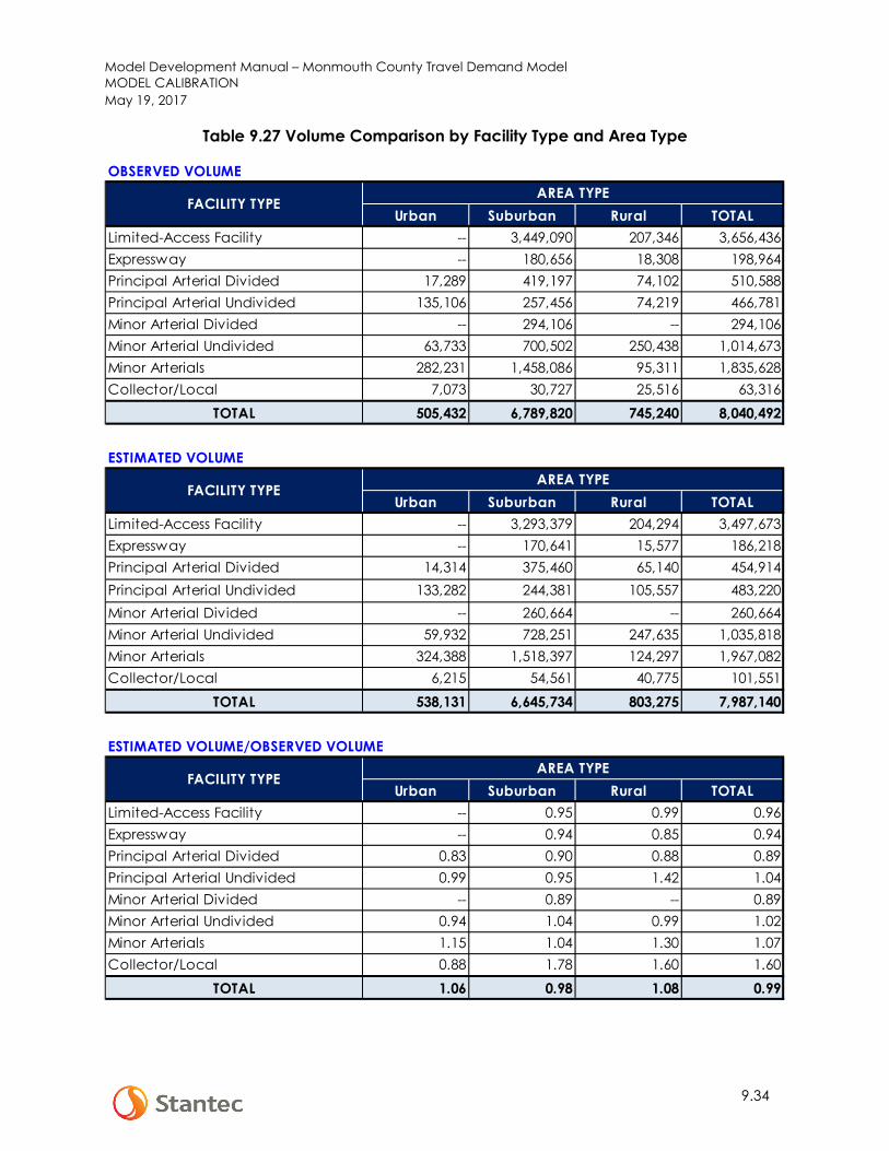
Model Development Manual – Monmouth County Travel Demand Model MODEL CALIBRATION May 19, 2017
9.34
Table 9.27 Volume Comparison by Facility Type and Area Type
OBSERVED VOLUME
Urban Suburban Rural TOTALLimited-Access Facility -- 3,449,090 207,346 3,656,436Expressway -- 180,656 18,308 198,964Principal Arterial Divided 17,289 419,197 74,102 510,588Principal Arterial Undivided 135,106 257,456 74,219 466,781Minor Arterial Divided -- 294,106 -- 294,106Minor Arterial Undivided 63,733 700,502 250,438 1,014,673Minor Arterials 282,231 1,458,086 95,311 1,835,628Collector/Local 7,073 30,727 25,516 63,316
TOTAL 505,432 6,789,820 745,240 8,040,492
ESTIMATED VOLUME
Urban Suburban Rural TOTALLimited-Access Facility -- 3,293,379 204,294 3,497,673Expressway -- 170,641 15,577 186,218Principal Arterial Divided 14,314 375,460 65,140 454,914Principal Arterial Undivided 133,282 244,381 105,557 483,220Minor Arterial Divided -- 260,664 -- 260,664Minor Arterial Undivided 59,932 728,251 247,635 1,035,818Minor Arterials 324,388 1,518,397 124,297 1,967,082Collector/Local 6,215 54,561 40,775 101,551
TOTAL 538,131 6,645,734 803,275 7,987,140
ESTIMATED VOLUME/OBSERVED VOLUME
Urban Suburban Rural TOTALLimited-Access Facility -- 0.95 0.99 0.96Expressway -- 0.94 0.85 0.94Principal Arterial Divided 0.83 0.90 0.88 0.89Principal Arterial Undivided 0.99 0.95 1.42 1.04Minor Arterial Divided -- 0.89 -- 0.89Minor Arterial Undivided 0.94 1.04 0.99 1.02Minor Arterials 1.15 1.04 1.30 1.07Collector/Local 0.88 1.78 1.60 1.60
TOTAL 1.06 0.98 1.08 0.99
FACILITY TYPEAREA TYPE
FACILITY TYPEAREA TYPE
FACILITY TYPEAREA TYPE

Model Development Manual – Monmouth County Travel Demand Model MODEL CALIBRATION May 19, 2017
9.35
Table 9.28 RMSE Comparison by Volume Group
The next comparison is traffic volume by screenline. Figure 9.16 shows the screenline locations for this study, while Table 9.29 shows the total traffic by screenline.
> 80,000 12.0 16.070,000-80,000 16.6 16.060,000-70,000 11.7 18.050,000-60,000 21.9 20.040,000-50,000 -- 21.030,000-40,000 13.7 23.020,000-30,000 37.7 25.010,000-20,000 41.1 27.0
0-10,0000 55.9 40-60TOTAL 41.0 35-40
VOLUME GROUPMODEL
ESTIMATED RMSE
FHWA STANDARD

Model Development Manual – Monmouth County Travel Demand Model MODEL CALIBRATION May 19, 2017
9.36
Figure 9.16 Screenline Definition

Model Development Manual – Monmouth County Travel Demand Model MODEL CALIBRATION May 19, 2017
9.37
Table 9.29 Total Screenline Traffic Comparison
The distribution of screenline traffic among the roadways is shown in Table 9.30. At this level, the difference between observed and estimated traffic is more pronounced as expected.
Screenline No Observed Counts
Estimated Volumes Ratio
Screenline 1 532,390 571,200 1.07Screenline 2 97,268 152,063 1.56Screenline 3 125,926 157,211 1.25Screenline 4 217,001 215,488 0.99Screenline 5 321,046 352,843 1.10Screenline 6 263,048 230,648 0.88Screenline 7 536,700 537,322 1.00Screenline 8 110,436 115,419 1.05Screenline 9 196,025 207,562 1.06
Screenline 10 72,313 99,071 1.37Screenline 11 322,895 269,572 0.83Screenline 12 181,817 172,117 0.95Screenline 13 347,466 294,092 0.85Screenline 14 96,340 74,136 0.77
Total 3,420,671 3,448,745 1.01

Model Development Manual – Monmouth County Travel Demand Model MODEL CALIBRATION May 19, 2017
9.38
Table 9.30 Individual Roadway Comparison by Screenline
ScreenLine Location Observed Counts Distribution Estimated
Volumes Distribution Ratio
CR-526/Robinsville Allentown Rd 9,004 1.7% 31,651 5.5% 3.52I-195 63,637 12.0% 41,337 7.2% 0.65Old York Rd 6,551 1.2% 8,615 1.5% 1.32CR-571/Etra Perineville Rd 3,919 0.7% 7,835 1.4% 2.00NJ-33 34,181 6.4% 41,815 7.3% 1.22CR-522 (N of Spotswood Englishtown Rd) 6,945 1.3% 9,890 1.7% 1.42CR-527/Old Bridge Englishtown Rd 10,173 1.9% 10,471 1.8% 1.03CR-520/Texas Rd 13,716 2.6% 11,766 2.1% 0.86NJ-18 39,948 7.5% 49,996 8.8% 1.25US-9 77,040 14.5% 84,642 14.8% 1.10Ticetown Rd 1,451 0.3% 10,053 1.8% 6.93CR-516/Old Bridge Matawan Rd 4,298 0.8% 10,289 1.8% 2.39CR-689/Amboy Rd 5,066 1.0% 7,884 1.4% 1.56NJ-34 25,466 4.8% 39,526 6.9% 1.55CR-6A/Ravine Dr 5,104 1.0% 4,777 0.8% 0.94Garden State Parkway 180,990 34.0% 172,742 30.2% 0.95NJ-35 38,182 7.2% 22,920 4.0% 0.60Amboy Rd 6,719 1.3% 4,991 0.9% 0.74
532,390 100.0% 571,200 100.0% 1.07CR-524 6,387 6.6% 10,999 7.2% 1.72CR-28/Old York Rd 3,399 3.5% 8,567 5.6% 2.52CR-537/Monmouth Rd 6,347 6.5% 15,296 10.1% 2.41CR-528/Jacobstown New Egypt Rd 4,504 4.6% 4,413 2.9% 0.98CR-616/Cookstown New Egypt Rd 5,782 5.9% 5,505 3.6% 0.95Bunting Bridge Rd 1,556 1.6% 277 0.2% 0.18NJ-70 11,083 11.4% 11,327 7.4% 1.02NJ-72 8,891 9.1% 15,298 10.1% 1.72Garden State Parkway 39,733 40.8% 73,809 48.5% 1.86US-9 9,586 9.9% 6,572 4.3% 0.69
97,268 100.0% 152,063 100.0% 1.56CR-527A/Iron Ore Rd 3,816 3.0% 5,780 3.7% 1.51Woodward Rd 9,572 7.6% 5,781 3.7% 0.60NJ-33 27,727 22.0% 45,909 29.2% 1.66CR-527/Sweetmans Ln 11,634 9.2% 7,263 4.6% 0.62Oakland Mills Rd 1,146 0.9% 4,546 2.9% 3.97Monmouth Rd 20,269 16.1% 22,744 14.5% 1.12Ely Harmony Rd 2,280 1.8% 5,468 3.5% 2.40I-195 49,482 39.3% 59,721 38.0% 1.21
125,926 100.0% 157,211 100.0% 1.25CR-516/New Brunswick Ave 9,452 4.2% 10,430 5.0% 1.10Wilson Ave 4,490 2.0% 6,884 3.3% 1.53NJ-79 10,004 4.5% 7,842 3.8% 0.78Lloyd Rd 15,755 7.0% 12,167 5.8% 0.77CR-520/Newman Springs Rd 12,605 5.6% 10,399 5.0% 0.83Crine Rd 5,834 2.6% 5,812 2.8% 1.00CR-537 15,273 6.8% 14,493 6.9% 0.95NJ-18 47,666 21.2% 48,278 23.1% 1.01Asbury Rd 8,094 3.6% 9,196 4.4% 1.14Belmar Blvd 3,579 1.6% 4,497 2.2% 1.26CR-524 7,739 3.4% 5,949 2.9% 0.77I-195 65,719 29.2% 60,634 29.1% 0.92CR-549/Herbertsville Rd 15,077 6.7% 7,419 3.6% 0.49Lakewood Allenwood Rd 3,453 1.5% 4,620 2.2% 1.34
224,740 100.0% 208,619 100.0% 0.93
Scre
enlin
e 3
Scre
enlin
e 1
TOTAL
Scre
enlin
e 2
TOTAL
TOTAL
Scre
enlin
e 4
TOTAL

Model Development Manual – Monmouth County Travel Demand Model MODEL CALIBRATION May 19, 2017
9.39
Table 9.29 – Continued
NJ-36 23,861 7.4% 23,048 6.6% 0.97CR-516/Leonardville Rd 11,918 3.7% 10,982 3.1% 0.92Kings Hwy E 4,430 1.4% 11,719 3.4% 2.65Cooper Rd 987 0.3% 100 0.0% 0.10NJ-35 42,398 13.2% 34,072 9.8% 0.80W Front St 16,330 5.1% 29,231 8.4% 1.79CR-520/Newman Springs Rd 18,584 5.8% 25,668 7.4% 1.38CR-13A/Sycamore Ave 19,090 5.9% 16,413 4.7% 0.86Tinton Ave 18,075 5.6% 16,932 4.8% 0.94NJ-36 34,899 10.9% 40,877 11.7% 1.17CR-547/Wyckoff Rd 16,390 5.1% 16,503 4.7% 1.01Indistrial Way W 12,203 3.8% 10,033 2.9% 0.82W Park Ave 17067 5.3% 23,882 6.8% 1.40Deal Rd 11,583 3.6% 13,564 3.9% 1.17NJ-35 30,216 9.4% 28,806 8.2% 0.95Wickapecko Dr 5,574 1.7% 9,050 2.6% 1.62Asbury Ave 11,115 3.5% 7,780 2.2% 0.70Bangs Ave 2,684 0.8% 6,284 1.8% 2.34NJ-71/Main St 18,640 5.8% 20,141 5.8% 1.08Lake Terrace 5,002 1.6% 4,120 1.2% 0.82
321,046 100.0% 349,205 100.0% 1.09NJ-36/Memorial Pkwy 13,708 5.2% 19,893 8.6% 1.45Ridge Rd 5,526 2.1% 4,170 1.8% 0.75CR-520/Rumson Rd 12,494 4.7% 10,625 4.6% 0.85NJ-36 (Joline Ave) 23,082 8.8% 9,933 4.3% 0.43Broadway 11,381 4.3% 9,530 4.1% 0.84N Bath Ave (SE of High St) 9,915 3.8% 4,372 1.9% 0.44Westwood Ave (S of N Bath Ave) 6,563 2.5% 6,331 2.7% 0.96Cedar Ave (E of Westwood Ave) 11,905 4.5% 8,816 3.8% 0.74NJ-71/Norwood Ave (N of Roseld Ave) 14,799 5.6% 12,196 5.3% 0.82Grassmere Ave 2,604 1.0% 4,403 1.9% 1.69Asbury Ave 7,319 2.8% 6,951 3.0% 0.95Bangs Ave 2,684 1.0% 6,284 2.7% 2.34NJ-33 17,289 6.6% 14,314 6.2% 0.83NJ-35 16,823 6.4% 10,179 4.4% 0.61NJ-35/River Rd 27,442 10.4% 16,900 7.3% 0.6216th Ave 7,537 2.9% 7,627 3.3% 1.01CR-30/18th Ave 5,287 2.0% 9,293 4.0% 1.76CR-524/Allaire Rd 8,465 3.2% 9,673 4.2% 1.14Warren Ave (E of Old Mill Rd) 6,708 2.6% 6,112 2.6% 0.91Sea Girt Ave (E of Old Mill Rd) 9,217 3.5% 11,296 4.9% 1.23Atlantic Ave 9,842 3.7% 6,796 2.9% 0.69Old Bridge Rd 4,457 1.7% 7,850 3.4% 1.76NJ-35 22,000 8.4% 19,306 8.4% 0.88Riverview Dr 6,001 2.3% 7,800 3.4% 1.30
263,048 100.0% 230,648 100.0% 0.88
Distribution Distribution
TOTAL
Observed Counts
Estimated Volumes Ratio
Scre
enlin
e 6
TOTAL
ScreenLine Location
Scre
enlin
e 5

Model Development Manual – Monmouth County Travel Demand Model MODEL CALIBRATION May 19, 2017
9.40
Table 9.29 – Continued
ScreenLine Location Observed Counts Distribution Estimated
Volumes Distribution Ratio
Ely Harmony Rd 532 0.1% 3,571 0.7% 6.71CR-527/Siloam Rd 10,960 2.0% 9,257 1.7% 0.84CR-524 (E of Gravel Hill Rd) 13,996 2.6% 13,857 2.6% 0.99Stillwells Corner Rd 10,016 1.9% 9,844 1.8% 0.98US-9 54,084 10.1% 56,379 10.5% 1.04NJ-33 30,472 5.7% 31,010 5.8% 1.02NJ-33 (Park Ave) 10,610 2.0% 13,379 2.5% 1.26CR-55/Kozloski Rd 23,074 4.3% 24,364 4.5% 1.06NJ-18 (S of Exit 22A) 47,666 8.9% 48,278 9.0% 1.01Five Points Rd 12,007 2.2% 9,193 1.7% 0.77CR-537 15,273 2.8% 14,493 2.7% 0.95Heyers Mill Rd (S of Flock Rd) 2,011 0.4% 3,625 0.7% 1.80NJ-34 16,639 3.1% 27,128 5.0% 1.63Swimming River Rd 10,318 1.9% 8,867 1.7% 0.86Garden State Parkway 170,600 31.8% 171,156 31.9% 1.00Hance Ave 9,436 1.8% 8,329 1.6% 0.88CR-13 /Shrewsbury Ave 31,867 5.9% 16,218 3.0% 0.51NJ-35/Broad St 22,033 4.1% 19,873 3.7% 0.90Branch Ave 11,680 2.2% 13,441 2.5% 1.15Prospect Ave 11,249 2.1% 9,061 1.7% 0.81Seven Bridges Rd 10,413 1.9% 12,076 2.2% 1.16NJ-36/Ocean Ave 11,764 2.2% 13,923 2.6% 1.18
536,700 100.0% 537,322 100.0% 1.00CR-530 (N of Dover Rd) 20,064 18.2% 11,453 9.9% 0.57Garden State Parkway 81,785 74.1% 95,756 83.0% 1.17Pinewald Rd (S of Birch St) 8,587 7.8% 8,209 7.1% 0.96
110,436 100.0% 115,419 100.0% 1.05I-195 49,482 25.2% 59,721 28.8% 1.21Jackson Mills Rd 9,172 4.7% 10,139 4.9% 1.11Bennetts Mills Rd 12,761 6.5% 6,257 3.0% 0.49E Veterans Hwy 10,365 5.3% 8,339 4.0% 0.80CR-527/Whitesville Rd 9,155 4.7% 11,404 5.5% 1.25CR-547/S Hope Chapel Rd 13,205 6.7% 12,145 5.9% 0.92CR-571/ Ridgeway Rd 12,244 6.2% 16,362 7.9% 1.34NJ-70 14,727 7.5% 10,653 5.1% 0.72NJ-37 30,130 15.4% 20,811 10.0% 0.69CR-530 20,064 10.2% 11,453 5.5% 0.57Dover Rd 1,168 0.6% 7,143 3.4% 6.12Lacey Rd 6,741 3.4% 4,579 2.2% 0.68CR-532/Warren Grove Rd (S of Jones Rd) 2,089 1.1% 6,924 3.3% 3.31CR-539/ Main St 4,722 2.4% 21,632 10.4% 4.58
196,025 100.0% 207,562 100.0% 1.06Highbridge Rd 2,898 4.0% 2,368 2.4% 0.82CR-539/Pinehurst Rd 13,051 18.0% 12,997 13.1% 1.00CR-640/Hawkin Rd 2,847 3.9% 2,952 3.0% 1.04I-195 39,990 55.3% 56,570 57.1% 1.41Cassville Rd 13,527 18.7% 24,184 24.4% 1.79
72,313 100.0% 99,071 100.0% 1.37
Scre
enlin
e 7
TOTAL
Scre
enlin
e 8
TOTAL
Scre
enlin
e 10
TOTAL
Scre
enlin
e 9
TOTAL
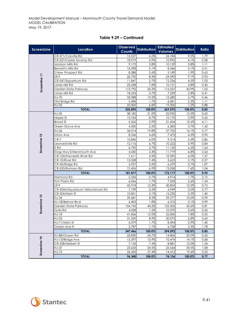
Model Development Manual – Monmouth County Travel Demand Model MODEL CALIBRATION May 19, 2017
9.41
Table 9.29 – Continued
CR-571/Casville Rd 13,527 4.2% 24,184 9.0% 1.79CR-527/Cedar Swamp Rd 18,919 5.9% 10,995 4.1% 0.58Jackson Mills Rd 9,172 2.8% 10,139 3.8% 1.11Bennetts Mills Rd 16,398 5.1% 8,346 3.1% 0.51S New Prospect Rd 8,388 2.6% 5,189 1.9% 0.62US-9 26,755 8.3% 24,590 9.1% 0.92CR-547/Squankum Rd 11,847 3.7% 12,236 4.5% 1.03Lanes Mill Rd 25,258 7.8% 10,151 3.8% 0.40Garden State Parkway 113,792 35.2% 115,537 42.9% 1.02Lanes Mill Rd 18,253 5.7% 7,539 2.8% 0.41NJ-70 33,088 10.2% 15,280 5.7% 0.46Old Bridge Rd 5,498 1.7% 6,081 2.3% 1.11NJ-35 22,000 6.8% 19,306 7.2% 0.88
322,895 100.0% 269,572 100.0% 0.83NJ-35 38,182 21.0% 22,920 13.3% 0.60Maple St 15,763 8.7% 10,170 5.9% 0.65Broad St 5,262 2.9% 21,604 12.6% 4.11Green Grove Ave 4,500 2.5% 6,385 3.7% 1.42NJ-36 36,014 19.8% 27,705 16.1% 0.77Union Ave 8,346 4.6% 7,473 4.3% 0.90CR-7 10,840 6.0% 9,314 5.4% 0.86Leonardville Rd 12,116 6.7% 10,222 5.9% 0.84E Rd 6,792 3.7% 11,150 6.5% 1.64Kings Hwy E/Monmouth Ave 4,430 2.4% 11,719 6.8% 2.65CR-12A/Navesink River Rd 7,611 4.2% 10,395 6.0% 1.37CR-10/River Rd 13,528 7.4% 3,623 2.1% 0.27CR-34/Ridge Rd 5,937 3.3% 6,379 3.7% 1.07CR-520/Rumson Rd 12,496 6.9% 13,058 7.6% 1.04
181,817 100.0% 172,117 100.0% 0.95Harmony Rd 2,336 0.7% 4,914 1.7% 2.10Fort Plains Rd 6,066 1.7% 7,533 2.6% 1.24US-9 42,918 12.4% 30,824 10.5% 0.72CR-524A/Squankum Yellowbrook Rd 7,739 2.2% 5,949 2.0% 0.77CR-524/Main St 10,851 3.1% 15,232 5.2% 1.40NJ-34 29,681 8.5% 29,277 10.0% 0.99NJ-18/Belmar Blvd 6,403 1.8% 6,310 2.1% 0.99Garden State Parkway 154,742 44.5% 125,305 42.6% 0.81Gully Rd 4,028 1.2% 10,570 3.6% 2.62NJ-18 41,836 12.0% 22,850 7.8% 0.55NJ-35 31,000 8.9% 20,075 6.8% 0.65NJ-71/Main St 6,079 1.7% 8,494 2.9% 1.40Ocean Ave N 3,787 1.1% 6,758 2.3% 1.78
347,466 100.0% 294,092 100.0% 0.85NJ-88/Ocean Rd 23,830 24.7% 14,806 20.0% 0.62NJ-13/Bridge Ave 15,297 15.9% 10,474 14.1% 0.68CR-528/Herbert St 7,143 7.4% 8,881 12.0% 1.24NJ-37 23,635 24.5% 25,564 34.5% 1.08NJ-72 26,435 27.4% 14,412 19.4% 0.55
96,340 100.0% 74,136 100.0% 0.77
RatioDistribution DistributionObserved Counts
Estimated Volumes
TOTAL
Scre
enlin
e 11
TOTAL
ScreenLine Location
Scre
enlin
e 14
TOTAL
Scre
enlin
e 12
TOTAL
Scre
enlin
e 13

Model Development Manual – Monmouth County Travel Demand Model MODEL CALIBRATION May 19, 2017
9.42
The final comparison for the highway assignment calibration is speed by time-of-day for various major highways within Monmouth County as shown in Table 9.31. The estimated speeds are generally within reasonable tolerance except for CR 35 and Route 79, in which the model estimated a higher speed than indicated by the observed data.
Table 9.31 Speed Comparison for Major Roadways
OBS EST PCT DIFF OBS EST PCT DIFFNorthbound 68 50 -27% 68 68 0%Southbound 69 63 -8% 68 68 0%Northbound 40 44 12% 35 45 26%Southbound 40 44 10% 35 45 28%Westbound 67 64 -5% 67 65 -3%Eastbound 67 59 -12% 67 65 -2%Westbound 46 48 4% 47 48 3%Eastbound 47 49 3% 47 49 4%
Northbound 66 65 -2% 63 64 1%Southbound 64 58 -10% 64 64 -1%Northbound 32 20 -38% 30 30 1%Southbound 33 27 -17% 30 33 9%Northbound 32 31 -3% 33 31 -5%Southbound 34 31 -11% 34 31 -8%Northbound 43 47 10% 42 47 13%Southbound 42 47 12% 42 47 14%Westbound 38 38 1% 36 38 8%Eastbound 38 39 0% 37 39 5%
Between I-195 and GSP
Between NJ TPK and RT 18
Between US 9 and CR 33
Between US 9 and County Line Rd.
Between RT 34 and RT 33
Between RT 79 and RT 35
Garden State Parkway
US 9
I-195
Road Name Direction AM Period Speed (mph) MD Period Speed (mph)Location
Between US 9 and Burnt Tavern Rd
Between RT 18 and Central Avenue
Between NJ TPK and GSP
CR 33
RT 537
RT 34
RT 79
CR 35
RT 18
OBS EST PCT DIFF OBS EST PCT DIFFNorthbound 68 62 -9% 66 69 4%Southbound 66 57 -14% 67 68 3%Northbound 33 44 33% 42 45 8%Southbound 33 44 34% 41 45 11%Westbound 66 53 -21% 66 65 0%Eastbound 68 63 -7% 66 66 -1%Westbound 45 47 5% 48 48 0%Eastbound 45 49 8% 48 49 1%
Northbound 65 56 -13% 63 66 3%Southbound 65 63 -4% 63 66 3%Northbound 28 25 -12% 34 19 -45%Southbound 28 19 -33% 34 14 -58%Northbound 31 31 2% 35 31 -11%Southbound 31 31 1% 37 31 -14%Northbound 40 47 15% 45 48 6%Southbound 39 47 18% 44 48 8%Westbound 33 37 11% 40 39 -1%Eastbound 35 37 5% 40 40 -1%
PM Period Speed (mph) NT Period Speed (mph)Road Name Location Direction
Garden State Parkway
Between US 9 and Burnt Tavern Rd
US 9Between RT 18 and
Central Avenue
I-195Between NJ TPK and
GSP
CR 33Between NJ TPK and RT
18
RT 18Between US 9 and CR
33
RT 537 Between I-195 and GSP
CR 35Between US 9 and County Line Rd.
RT 79Between RT 34 and RT
33
RT 34Between RT 79 and RT
35

Model Development Manual – Monmouth County Travel Demand Model MODEL CALIBRATION May 19, 2017
9.43
9.6 TRANSIT ASSIGNMENT CALIBRATION
Monmouth County has various transit lines that serve the county, including buses, trains, and ferries. Table 9.31 shows the transit ridership comparison by modes and lines.
Table 9.32 Transit Ridership Comparison
Observed Estimated64 325 23167 166 430133 556 47135 154 106139 3383 4711
Total 4,584 5,525
Line Name Bus Ridership
Observed EstimatedAberdeen-Matawan 2,460 1,560
Hazlet 874 1,179Middletown 1,331 1,083
Red Bank 1,155 798Little Silver 740 915
Long Branch 1,105 1,432Elberon 117 176
Allenhurst 125 67Asbury Park 548 430
Bradley Beach 225 395Belmar 256 333
Spring Lake 152 271Manasquan 175 260
Total 9,263 8,899
Station Name Rail Ridership
Observed EstimatedBelford 1916 2937
Atlantic Highlands 1863 1309Highlands 1417 1366
Total 5,196 5,612
Station NameFerry Ridership

Model Development Manual – Monmouth County Travel Demand Model MODEL CALIBRATION May 19, 2017
9.44
9.7 MODEL OUTPUTS
Each model component of the MCTDM produces a number of output files. Some of them are temporary and can be ignored, while others are either inputs of the following components or output files for review and summary. The major output files of each component are listed in Appendix C for reference.
In addition to the above output files, other important outputs are the period-specific output highway networks generated by the highway network assignment process. There are four time periods defined in the MCTDM as discussed in Chapter 9.1, including AM Peak, Midday, PM Peak, and Night. The highway assignment process generates a highway network file, also known as loaded highway network, for each time period. The loaded highway network includes additional link variables, or output link variables, as listed in Appendix D.
Model Development Manual – Monmouth County Travel Demand Model ADDITIONAL FEATURES May 19, 2017
10.1
10.0 ADDITIONAL FEATURES
10.1 SEASONAL MODEL
The seasonal model was developed to capture additional traffic demand for people traveling to the New Jersey shores during the summer months. The increase of summer traffic can be attributed to two categories:
• The increase of local activities. • The in-flux of long-distance trips from nearby regions, such as New York City, Philadelphia,
Trenton, and South Jersey. The increase of local-activities is assumed to be proportional with the vacation housing available in the area. Table 10.1 provides the percentage of seasonal housing by municipality. The data was obtained from the 2015 Housing Units Summary from the Census website. The percentage of vacation housing units were then converted from MCD-Level to TAZ-Level using an MCD-Zones equivalency table developed for this model.
The additional traffic from the local trips is calculated using the following formula:
Additional Local Trips for i-j cell = Average Daily Trips * the average of percent vacation housing units at location i and j
Only a portion of these trips are assumed to occur. Therefore, an adjustment factor is applied to these local trips. Currently, the factor is set to 0.50. The factor was determined with a trial and error approach to get the estimated trips replicating the very limited observed data.
The second component of the seasonal model is the in-flux on long distance trips. For the purpose of this model, Stantec assumed that there are five origin points for these trips:
• Garden State Parkway (GSP) for the Northern market such as NYC and North Jersey.
• Route 18 for the Northwestern market, such as North Jersey.
• I-195 and Route 33 for the Western market, such as Trenton and Central Jersey.
• GSP for the Southern market, such as South Jersey.
Figure 10.1 shows the proximity of these locations.

Model Development Manual – Monmouth County Travel Demand Model ADDITIONAL FEATURES May 19, 2017
10.2
Table 10.1 Vacation Housing Percentage by MCD in Monmouth
MCD Vacation House Percentage MCD Vacation House
Percentage
Aberdeen township 0.0% Long Branch city 9.0%Allenhurst borough 0.0% Manalapan township 0.0%Allentown borough 0.0% Manasquan borough 21.2%Asbury Park city 3.3% Marlboro township 0.0%Atlantic Highlands borough 0.0% Matawan borough 0.0%Avon-by-the-Sea borough 0.0% Middletown township 0.8%Belmar borough 21.4% Millstone township 0.0%Bradley Beach borough 0.0% Monmouth Beach borough 20.7%Brielle borough 0.0% Neptune township 8.1%Colts Neck township 0.0% Neptune City borough 0.0%Deal borough 58.5% Ocean township 4.0%Eatontown borough 0.0% Oceanport borough 0.0%Englishtown borough 0.0% Red Bank borough 0.0%Fair Haven borough 0.0% Roosevelt borough 0.0%Farmingdale borough 0.0% Rumson borough 0.0%Freehold borough 0.0% Sea Bright borough 26.6%Freehold township 0.0% Sea Girt borough 0.0%Hazlet township 0.0% Shrewsbury borough 0.0%Highlands borough 8.1% Shrewsbury township 0.0%Holmdel township 0.0% Spring Lake borough 0.0%Howell township 0.0% Spring Lake Heights borough 23.8%Interlaken borough 0.0% Tinton Falls borough 0.0%Keansburg borough 0.0% Union Beach borough 0.0%Keyport borough 0.0% Upper Freehold township 0.0%Lake Como borough 0.0% Wall township 3.9%Little Silver borough 0.0% West Long Branch borough 0.0%Loch Arbour village 0.0%

Model Development Manual – Monmouth County Travel Demand Model ADDITIONAL FEATURES May 19, 2017
10.3
Figure 10.1 Seasonal Traffic Flow Pattern - Inbound
The five seasonal TAZs are as follows:
• TAZ 1111 - represents the origin point of the Northern market such as NYC/North Jersey.
• TAZ 3013 – represents the origin point of the Northwestern market, such as North Jersey.
• TAZs 954 and 1335 – represents the origin point of the Western market, such as Central NJ
and Trenton.
• TAZ 3161 – represents the origin point of the Southern market, such as South Jersey.

Model Development Manual – Monmouth County Travel Demand Model ADDITIONAL FEATURES May 19, 2017
10.4
As the first step of the long-haul seasonal traffic estimation, Stantec gathered traffic count information from NJDOT’s permanent stations and Garden State Parkway that can be used as proxy for these locations. There were very limited traffic counts that can be used for this purpose, since the counts should have both average daily counts, as well as counts for summer months by direction. Table 10.2 shows the comparison between high summer traffic volumes and AADT for the selected locations. Since there is no permanent count available on I-195, Stantec utilized the NJDOT’s seasonal factor to convert the AADT into Summer Counts.
Table 10.2 High Summer Month and AADT Traffic Comparison
The average additional summer traffic from Table 10.2 was used as the base for the long-haul trip production, and is summarized in Table 10.3. Additional adjustment factors were added to account for the discrepancy between the seasonal TAZ locations (shown in Figure 10-2) and the locations of the count, such that the estimated additional summer traffic replicate the observed data. The adjustment factors are listed in Table 10.4.
Table 10.3 Long-Haul In-Bound Trip Origin
North (GSP) 25,234Northwest (RT 18) 3,569
West (RT 33) 1,259West (I-195) 3,287South (GSP) 15,865
LocationAverage
Additional Summer Traffic
High Summer Volume AADT
Additional Summer Traffic
High Summer Volume AADT
Additional Summer Traffic
GSP at Exit 120 114,793 88,987 25,806 109,704 85,042 24,662 25,234RT 18 east of Route 9 16,072 12,503 3,569 16,072 12,503 3,569 3,569
RT 33 east of NJ Turnpike 8,299 7,040 1,259 8,300 7,041 1,259 1,259I-195 east of NJ Turnpike 33,185 29,966 3,219 34,577 31,223 3,354 3,287GSP north of Route 88 72,160 55,938 16,222 68,985 53,477 15,508 15,865
Average Additional
Summer Traffic
In-Bound Out-Bound
Location

Model Development Manual – Monmouth County Travel Demand Model ADDITIONAL FEATURES May 19, 2017
10.5
Table 10.4 Adjustment Factors In-Bound Trip Origin
The attraction of the long-haul in-bound summer traffic was also estimated based on vacation housing units. The distribution of the trips from the four production zones to all potential attraction zones, zones with vacation housing, was performed using a simple gravity model with trips balanced to production.
The out-bound trips, which represent the return trips on Sunday, were calculated using similar approach as the in-bound trips. However, the production and attraction were reversed and the trips are balanced to attraction.
The daily seasonal trips were distributed into four time-of-day, AM, PM, Midday, and Night using the time of day factors developed from the GSP hourly summer traffic counts at five toll plazas are shown in Table 10.5
Table 10.5 Time-Of-Day Factors for Seasonal Trips
Toll Location AM MD PM NT TOTALNew Gretna NB (Inbound) 2,289 15,217 6,306 12,825 36,637 Barnegat SB (Outbound) 5,901 22,033 11,914 13,003 52,851 Toms River NB (Inbound) 4,439 25,705 12,106 23,903 66,153
Toms River SB (Outbound) 8,194 27,407 13,614 16,688 65,903 Asbury Park NB (Outbound) 6,485 40,782 22,027 41,064 110,358
Raritan Toll Plaze SB (Inbound) 15,013 64,703 38,820 47,545 166,081 Inbound Total 21,741 105,625 57,232 84,273 268,871
Outbound Total 20,580 90,222 47,555 70,755 229,112
Inbound Time-Of-Day Factors8.1% 39.3% 21.3% 31.3%
Outbound Time-of-Day Factors 9.0% 39.4% 20.8% 30.9%
North (GSP) 1Northwest (RT 18) 1
West (RT 33) 1West (I-195) 1South (GSP) 1
LocationProduction Adjustment
Factors

Model Development Manual – Monmouth County Travel Demand Model ADDITIONAL FEATURES May 19, 2017
10.6
Table 10.6-10.9 tables show traffic comparison between traffic counts and the estimated volumes at selected locations for inbound and outbound by facility type and area type respectively. In general, the estimated volumes are reasonably close. A sample of daily seasonal traffic pattern is shown in Figure 10.2.
Table 10.6 Inbound Seasonal Traffic Comparison by Facility Type
Table 10.7 Inbound Seasonal Traffic Comparison by Area Type
Table 10.8 Inbound Seasonal Traffic Comparison by Facility Type
OBSERVED ESTIMATED EST/OBSLimited-Access Facility 767,136 897,690 1.17Expressway 41,692 41,501 1.00Principal Arterial Divided 29,932 26,625 0.89Principal Arterial Undivided 69,278 46,413 0.67Minor Arterial Divided 10,553 14,911 1.41Minor Arterial Undivided 66,126 66,381 1.00Minor Arterials 116,569 108,210 0.93Collector/Local 3,362 5,220 1.55
TOTAL 1,104,648 1,206,951 1.09
FACILITY TYPEVOLUME
OBSERVED ESTIMATED EST/OBSUrban 76,129 63,007 0.83
Suburban 881,137 871,870 0.99Rural 147,382 272,074 1.85TOTAL 1,104,648 1,206,951 1.09
AREA TYPEVOLUME
OBSERVED ESTIMATED EST/OBSLimited-Access Facility 766,895 902,118 1.18Expressway 38,632 46,686 1.21Principal Arterial Divided 29,934 27,473 0.92Principal Arterial Undivided 66,330 50,328 0.76Minor Arterial Divided 10,553 15,049 1.43Minor Arterial Undivided 57,240 65,564 1.15Minor Arterials 116,498 111,315 0.96Collector/Local 3,363 3,680 1.09
TOTAL 1,089,445 1,222,213 1.12
FACILITY TYPEVOLUME

Model Development Manual – Monmouth County Travel Demand Model ADDITIONAL FEATURES May 19, 2017
10.7
Table 10.9 Inbound Seasonal Traffic Comparison by Area Type
Figure 10.2 Daily Seasonal In-Bound Traffic Pattern for 2015 Model Year
OBSERVED ESTIMATED EST/OBSUrban 76,130 67,799 0.89
Suburban 861,779 885,848 1.03Rural 151,536 268,566 1.77TOTAL 1,089,445 1,222,213 1.12
AREA TYPEVOLUME
Traffic Increase Traffic Decrease

Model Development Manual – Monmouth County Travel Demand Model ADDITIONAL FEATURES May 19, 2017
10.8
For future year analysis, Stantec assumes that the long-haul traffic grows at a rate of 2% per year. This assumption considered that Hurricane Sandy hit the Jersey Shore in 2012 and impacted travel to Jersey Shore during that year. To minimize the impact of hurricane Sandy on the calculation, the growth rate was calculated using post Sandy traffic count data along the GSP at five mainline locations. Table 10.10 shows the historical growth rates at these locations:
Table 10.10 Historical Growth Rate along GSP
Note: (1) ACGR = Annual Compounded Growth Rate
To account for the growth, the analyst has to input the analysis year for the seasonal model. The year has to be input into SEASON_YR key variable as shown in Figure 10.4.
Figure 10.3 SEASON_YR Key Variable Input Window
% CAGR(1)
2013 2015 2013-2015NB 26,840 25,820 -1.9%SB 27,700 26,650 -1.9%NB 43,840 43,720 -0.1%SB 41,160 41,060 -0.1%NB 56,020 59,250 2.8%SB 52,780 56,190 3.2%NB 96,190 99,150 1.5%SB 98,120 101,140 1.5%NB 154,220 164,530 3.3%SB 132,840 141,710 3.3%NB 377,110 392,470 2.0%SB 352,600 366,750 2.0%
Two-way 729,710 759,220 2.0%
Average Highest Summer Month Daily TrafficToll Location Dir
Toms River
New Gretna
Barnegat
Asbury Park
Raritan
TOTAL

Model Development Manual – Monmouth County Travel Demand Model ADDITIONAL FEATURES May 19, 2017
10.9
10.2 OTHER SUPPORT APPLICATIONS
In addition to the Seasonal Model described in Chapter 10.1, the MCTDM includes a series of support applications that will help to prepare input data and summarize the model outputs. The list of the support applications is shown in Table 10.11.
Table 10.11 Support Applications
10.2.1 Transit Walk-Access Coverage
Access Processing support application is developed to estimate the percentage of each TAZ within transit walk-access coverage. This data is required for the mode choice model component and should be estimated when significant changes to the transit network are implemented. As an example, the walk coverage should be re-estimated if a scenario extends (or truncates) a transit route, or if new stations and boarding points are added. In preparation for this estimation, the background highway layer is merged with additional data from the transit input card files. The user then needs to execute the transit accessibility process in the CUBE environment. Finally, access coverage data is processed and zonal coverage is updated. Note that the execution of this particular application is performed manually by the model user. Detail discussion about this support application is provided in the Users’ Guide Manual.
Support Application Description
Transit Walk Access CoverageEstimates the percentage of each zone within transit walk-access - this application is needed to adjust the accessibility to transit in case there are route changes, or addition/removal certain transit routes, in the future.
NYMTC Trip ProcessingGenerates mode shares for the NYMTC-controlled region by using the person trips data by mode from the NYMTC BPM model.
Subarea Processing Helps extract network and trip tables for a customized subarea.
Fixed Distribution AnalysisSupports scenarios where it may be necessary to retain a common or fixed distribution of person trips.
Summary Preparation ProcessSummarizes the travel characteristics like average travel time and distance between counties, municipatlities, etc. by time of day.
Daily Network Statistics Prepares a loaded network with daily statistics, including transit link volumes.SED Conversion from NJRTM-E Facilitate the SED (Socioeconomic Data) conversion from NJRTM-E TAZs to Monmouth
Growth FactorCalculates the annual growth between model years or scenarios for all roadways in the network.
Critical Locations Identifies roadway corridors with congestion problems.PT Accessibility Display Tool Prepares a series of shape files for transit accessibility-related display.
Seasonal ModelEstimates the seasonal increase or decrease in traffic, especially trips to and from the Jersey shore during the summer months.
Dynamic Traffic Assignment with Cube Avenue
Prepares the model output for dynamic traffic assignment (using Cube Avenue). I t should be noted that Cube Avenue license is sold separately by Citilabs, and currently is not in our contract.

Model Development Manual – Monmouth County Travel Demand Model ADDITIONAL FEATURES May 19, 2017
10.10
10.2.2 NYMTC Trip Processing
This application is utilized to generate the mode shares for the NYMTC-controlled region from the NYMTC’s Best Practice Model (BPM) person trips by mode tables. A file in DBF format of county-level person trips by mode from NYMTC BPM model is initially converted to Voyager matrix format and mode shares are then calculated for each mode. Unreasonable auto shares are checked and resolved in a subsequent routine. Finally, county-level mode shares are expanded to zonal level and mode shares in the NJT controlled area are set to be zeros. To maintain consistency between the NJRTM-E and the County Model, the NYMTC mode shares update is usually performed at the NJRTM-E level and the results are shared with the County Model. This application is rarely used by the County Model. Additional information is provided in the Users’ Guide Manual.
10.2.3 Subarea Processing
A customized subarea extraction process is also provided as a standard output support application in the MCTDM. A model user can extract a subarea network and trip tables within a customized subregion within the MCTDM geographical area. This application is particularly useful if an analyst needs to perform a more detailed corridor analysis using a microscopic or mesoscopic model. The extracted subarea networks and trip tables are used as an input to these models. This application is discussed further in the Users’ Guide Manual.
10.2.4 Fixed Distribution Analysis
The fixed distribution analysis application was developed for scenarios where it would be necessary to retain a common or “Fixed” distribution of person trips. A few examples of those scenarios including traffic impact study for temporary roadway closures, build and no-build impact analysis for small projects, etc. The advantage of this approach is to avoid performing a lengthy model run.
To provide the maximum amount of flexibility, the user is permitted to control the specific model components that will be executed for each scenario. This will enable the user to perform only those elements of the model that are deemed necessary for the type and level of analysis desired, thereby minimizing execution time. As an example, if a user was investigating a scenario that featured a widening of a minor roadway that did not provide transit service, the user might wish to avoid executing the transit model components and the mode choice component. In contrast, if a major new transit facility was being developed, the user may wish to see the full impact of this project and therefore would execute both the highway and transit components of the model. This application is discussed further in the Users’ Guide Manual.

Model Development Manual – Monmouth County Travel Demand Model ADDITIONAL FEATURES May 19, 2017
10.11
10.2.5 Summary Preparation Process
This application was originally developed for the NJRTM-E and was retained in the MCTDM. The application summarizes the aggregated travel characteristics, such as average travel time and distance between counties by time of day (peak and off-peak), average time and distance from an MCD to others, and from others to an MCD. This application is discussed further in the Users’ Guide Manual.
10.2.6 Daily Network Statistics
This application generates a daily loaded network and its pertinent statistics, such as total daily volumes, traffic volumes by time period, etc. Transit link volumes are merged to the loaded network as well so that the transit travel pattern can be viewed visually in CUBE environment. Summary statistics including vehicle-miles of travel (VMT) and vehicle-hours of travel (VHT) are produced in the last routine. This application is discussed further in the Users’ Guide Manual.
10.2.7 SED Conversion from NJRTM-E
The MCTDM was developed based on the NJRTM-E’s model structure. However, the MCTDM has more refined TAZ system than the NJRTM-E’s system. This application was developed to facilitate the SED conversion from the NJRTM-E’s system to the MCTDM’s system. In the future, if Monmouth County decides to adopt the new and updated NJRTM-E’s socioeconomic data, this application can be used to convert the NJRTM-E’s socioeconomic data into the MCTDM’s data. This application is discussed further in the Users’ Guide Manual.
10.2.8 Growth Factors
This application was developed to calculate the roadways’ growth rates between the two model years or scenarios, for example the growth rates between 2015 and 2025, can be calculated using the 2015 and 2025 model year’s outputs. This application is discussed further in the Users’ Guide Manual.
10.2.9 Critical Locations
This application can be used to identify any roadway corridors that experience some congestion problems. The congested corridors were defined as those that have V/C ratio of 0.9 or higher. The congestion criteria can be adjusted as necessary by the users. Additional discussions are provided in the Users’ Guide Manual.

Model Development Manual – Monmouth County Travel Demand Model ADDITIONAL FEATURES May 19, 2017
10.12
10.2.10 Public Transit (PT) Accessibility Display Tool
PT Accessibility Display application is a tool to display various TAZs that have transit-accessibility to selected TAZs. For example, this application can be used to display all TAZs that can reach Freehold via transit. This application is discussed in detail in the Users’ Guide Manual.
10.3 FUTURE YEAR SCENARIOS
Two future year scenarios are prepared as part of this project, including 2025 and 2040. The future year highway networks were developed by implementing a series of future projects to the base year network. The future projects include transportation projects within Monmouth County as well as projects in the immediate surrounding counties that may impact traffic in Monmouth County. The surrounding counties include Mercer, Burlington, Ocean, and Middlesex. The list of future projects were obtained from the FY 2015 NJTPA’s Conformity Project list and shown in Table 10.12. All future projects obtained from the NJTPA’s Conformity Project list for these counties will be completed by 2025. There is no project that will be completed beyond 2025, Therefore, the 2025 highway network is identical with the 2040 highway network.

Model Development Manual – Monmouth County Travel Demand Model ADDITIONAL FEATURES May 19, 2017
10.13
Table 10.12 Future Project List

Model Development Manual – Monmouth County Travel Demand Model ADDITIONAL FEATURES May 19, 2017
10.14
Table 10.12 - Continued

Model Development Manual – Monmouth County Travel Demand Model ADDITIONAL FEATURES May 19, 2017
10.15
Table 10.12 - Continued
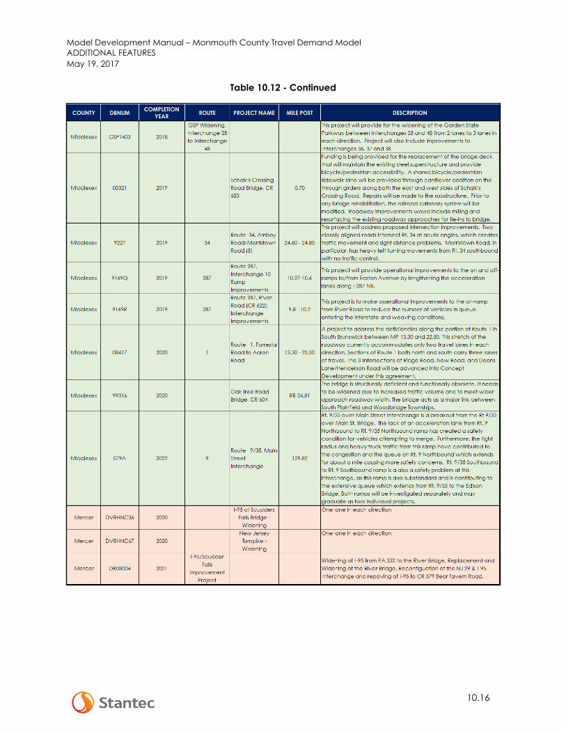
Model Development Manual – Monmouth County Travel Demand Model ADDITIONAL FEATURES May 19, 2017
10.16
Table 10.12 - Continued

Model Development Manual – Monmouth County Travel Demand Model ADDITIONAL FEATURES May 19, 2017
10.17
Table 10.12 - Continued
The future socioeconomic data was provided by NJTPA as shown previously in Table 2.2 and Table 2.3. The base year and future years Vehicle Miles Traveled (VMT) comparison by facility type and their compounded annual growth rates (CAGR) are presented in Table 10.13. The VMT in Monmouth County increases approximately 0.3% per year between 2015 and 2025, and 0.4% per year between 2025 and 2040.

Model Development Manual – Monmouth County Travel Demand Model ADDITIONAL FEATURES May 19, 2017
10.18
Table 10.13 Base Year and Future Years VMT Comparison by Facility Type
2015 2025 CAGR 2015-2025 2040 CAGR
2025-2040Limited-Access Facility 6,320,267 6,500,038 0.3% 7,055,549 0.5%Expressway 323,372 323,975 0.0% 349,751 0.5%Principal Arterial Divided 1,590,850 1,634,793 0.3% 1,737,411 0.4%Principal Arterial Undivided 1,087,483 1,109,471 0.2% 1,180,405 0.4%Minor Arterial Divided 711,491 733,966 0.3% 777,423 0.4%Minor Arterial Undivided 2,609,485 2,729,127 0.4% 2,916,061 0.4%Minor Arterials 3,932,937 4,069,168 0.3% 4,291,393 0.4%Collector/Local 997,327 1,041,486 0.4% 1,120,883 0.5%
TOTAL 17,573,212 18,142,024 0.3% 19,428,876 0.5%
FACILITY TYPEVMT

Model Development Manual – Monmouth County Travel Demand Model APPENDIX A – HIGHWAY NETWORK VARIABLES May 19, 2017
A.1
APPENDIX A – HIGHWAY NETWORK VARIABLES
PHYSICAL / OPERATIONAL VARIABLES
VARIABLE NAME DESCRIPTION UNIT DEFINITIONA A Node of a highway link IntegerB B Node of a highway link IntegerDISTANCE Distance of a highway link Miles
Define by a look up table, a function of area type and facility type, unless overriden by uservia FIXCAP FT is divided into 12 categories:1. Freeway (limited access)
3. Principal arterial divided4. Principal arterial undivided5. Major arterial divided6. Major arterial undivided7. Minor arterial8. Collector/local
10. Medium speed ramp (40 mph)11. Low speed ramp/jughandle (25 mph)12. Centroid connectorAT is divided into 5 categories1. CBD2. Urban3. Suburban4. Rural
LANESAM Number of lanes - AM Peak Integer Number of lanes in the AM Peak period. LANESPM Number of lanes - PM Peak Integer Number of lanes in the PM Peak period. LANESOP Number of lanes - Off Peak Integer Number of lanes in the Off Peak period.
Linktype is divided into 16 categories:1. Free - all2. Free - auto only3. Free - truck only4. Urban toll - all5. Urban toll - auto only6. Urban toll - truck only7. Rural toll - all8. Rural toll - auto only9. Rural toll - truck only10. Urban free - HOV only11. Urban toll - HOV only12. Urban toll - SOV, free HOV13. Urban toll, free HOV14. ETC only - all15. ETC only - auto only16. ETC only SOV and truck toll, free HOV
Terrain Type. Default terrain type is Tertype is divided into 3 categories:defined based on counties and 1. Levelfacility type: 2. Rolling- Rolling Terrain: Sussex, Warren 3. Mountainous Morris, Passaic, Hunterdon, Somerset, Rockland, Orange, Lackawanna, Wayne, Sullivan, and Luzerne- Mountainous: none- Level: all other counties and highways
TERTYPE Integer from 1 to 3
Integer from 1- to 4Area typeAT
LINKTYPELink permission code to utilize the link based on auto mode and toll
Integer from 1 to 16
2. Expressway (grade separated at major facilities, signals at minor facilities)
9. High speed ramp (direct freeway-freeway 55 mph)
CAPACITY
FT Facility type
Hourly lane capacity VPH
Integer from 1 to 12

Model Development Manual – Monmouth County Travel Demand Model APPENDIX A – HIGHWAY NETWORK VARIABLES May 19, 2017
A.2
VARIABLE NAME DESCRIPTION UNIT DEFINITIONNLTLANE Number of left turn lanes Default=0 NRTLANE Number of right turn lanes Default=0 LWIDTH Lane width Feet Default=12 feet
0 = Shoulder substandard or missing1 = Standard shoulder (default)TCD is divided into 13 categories:1. Two-way stop2. All-way stop3. Yield4. Ramp-meter5. Signal-uncoordinated-actuated6. Signal-uncoordinated-fixed7. Signal-coordinated-restricted progression8. Signal-coordinated-favorable progression9. Signal-coordinated-maximum progression10. Freeway diverge point11. Freeway merge point12. Uncontrolled - Shape Point99. UnknownUser-specified, program will assume=1if the value is not provided and TCD=5-9User-specified, program default if the the value is providedSIGCOR is divided into 3 categories:0. Uncoordinated Signal (Default)1. Coord-unfavorable2. Coord-favorable3. Coord-max
GC Green time/cycle ratio Share of green time/cycleAlpha coefficient for Volume DelayFunction in assignmentBeta coefficient for Volume Delay Function in assignmentDelay factor in HCM approximationof TCD-related delay
Program will provide default based on areatype and facility type.0 = not fixed (default)1 = fixed capacity to specific value, retains settings of TCD, GC0 = not fixed (default)1 = fixed
TOLL Toll values - actual placement Dollars For toll diversion highway assignmentScaled toll values to balance by 0 = no toll (default)direction 1 = non-directional toll
-0.5 and 0.5 = directional toll0 = default1 = set HOV toll to 02 = set truck toll to 00= no toll (default)1-98 = obtained from lookup table99 = toll value coded on link directly
TOLLFACAM Base toll factor for AM Period default =1TOLLFACPM Base toll factor for PM Period default =1TOLLFACMD Base toll factor for Mid-Day Period default =1TOLLFACNT Base toll factor for Night Period default =1
0 = not fixed 1 = fixed toll (default)
TOLLAPC Toll applied to vehicle types Flag
FIXTIME
MCTOLL Flag
SIGCOR Signal coordination Integer from 0 to 3
ALCOEF
FIXTOLL Fix Toll Flag
Calculated by programJFACT
JAFACT
ACCPT
FIXCAP
Delay factor for Akcelik Formula
TOLLCLASS Toll class for lookup system Integer from 0-99
Calculated by program
Fix capacity Flag
Fix Time Flag
Number of access point
Calculated by program
BTCOEF
NSIG Number of signal in the link Integer
SIGCYC Signal cycle Secs
Calculated by program
Traffic Control Devices Integer from 1 to 12, 99
Standard shoulder availableLSHOULD Flag
TCD

Model Development Manual – Monmouth County Travel Demand Model APPENDIX A – HIGHWAY NETWORK VARIABLES May 19, 2017
A.3
IDENTIFICATION VARIABLES
VARIABLE NAME DESCRIPTION UNIT DEFINITIONPARK is divided into 2 categories:1. Permitted parking - default values for FT=7 and AT=1,2; FT=8 and AT=1,2,30. Not permitted - default for others1 = additional queueing function is permitted in the volume delay function0 = no additional queueing function is used
ZDELAY Initial delay due to TCD Calculated by programADDDELAY Additional delay applied to the link Mins Optional field - NJ Transit (not used)
Calculated by program, but user can overridevia FIXTIME parameter0 = standard roadway (default)1 = XBL2= bus queue jump 9= exclusive bus link (BRT)Other codes available0 = standard roadway (default)1 = XBL2= bus queue jump 9= exclusive bus link (BRT)Other codes available
TADDAM Added time penalty to transit - AM Mins Link specific adjustment transit time - AMTADDOP Added time penalty to transit - OP Mins link specific adjustment transit time - OPTSCALEAM Transit time scaling factor - AM Systematic adjustment factor - AMTSCALEOP Transit time scaling factor - OP Systematic adjustment factor - OP
Flag 0-Walkable and pedestrian friendly0 or 1 1-Non-walkable
NONWALK Index of non-walkable link
T0 Free-flow travel time Mins
Flag
Flag
Transit travel time flag for AM PeakTCODEAM
TCODEOP Transit travel time flag for Off Peak
Calculated by program, but user can override
PARK Parking permission code Flag 0 or 1
QUEFLG Flag for queueing function Flag
SPEED Link speed
VARIABLE NAME DESCRIPTION UNIT DEFINITIONNAME Road name String Example: "New Jersey Turnpike"SRI Standard Route Identifier String Example: "00000095" for New Jersey TurnpikeBEGIN_MP Mile post of the beginning of the link MilesEND_MP Mile post of the end of the link MilesRT_LTR Route lettering String Example: "I-95" for New Jersey TurnpikeCOUNTY County FIPS code Integer
Conformity based project ID #obtained from NJTPA
REFZONE Zone where the link resides Integer
PROJN Integer

Model Development Manual – Monmouth County Travel Demand Model APPENDIX A – HIGHWAY NETWORK VARIABLES May 19, 2017
A.4
PERFORMANCE/USE VARIABLES
VARIABLE NAME DESCRIPTION UNIT DEFINITION1=NJTA2=Monmouth County3=NJDOT4=Ocean County Highway Network 2014 (only Amercom)5=Ocean County
COUNTS_TOT Total counts Integer Final countsCOUNTS_AUT Total auto counts Integer Final auto countsCOUNTS_TRK Total truck counts Integer Final truck countsCOUNTS_MTK Total medium counts if available Integer Final medium truck countsCOUNTS_HTK Total heavy counts if available Integer Final heavy truck countsSUMR_COUNT Summer counts if available Integer COUNT_YEAR The year of total counts Integer
AWDT AWDT counts indicator IntegerIf AWDT=1, the above counts represent AWDT counts. Otherwise, they represent AADT.
SOURCE The source of the counts Integer

Model Development Manual – Monmouth County Travel Demand Model APPENDIX B – INTERSECTION MODEL ASSUMPTIONS May 19, 2017
B.1
APPENDIX B – INTERSECTION MODEL ASSUMPTIONS
INTERSECTION TYPE:
There are five intersection types defined in the Intersection Model:
1. All-Way Stop 2. Two-Way Stop 3. Priority Intersection (Two-way Yield) Geometric 4. Fixed Signals Geometric 5. Gap Acceptance Roundabout
ALL-WAY STOP:
Default assumptions for the all-way stop parameters are as follows:
Attributes Values DescriptionApproach Nodes Location-based
First Arm Location-based
Lane Geometry As observed Use Aerial Photographs/Maps or other information such as NJ Straight Line Diagram
Minimum Capacity 100 Default Cube/Voyager value=1.0; Use 100 vehs/hr. (Professional judgment)
Randomness 1Default for unsignalized intersection; completely random, no coordination with other TCD
Use the following assumptions (professional judgment):
- Rural = 0.0
- Suburban = 0.1
- Urban = 0.2
- CBD = 0.3 All in secs./veh
Initial Queue 0 Assume No Initial Queue
Ban Turn As observed If information is not clear, always allow turn
Volumes Ignore
Use Aerial Photographs/Maps or other information such as NJ Straight Line Diagram. Number of Lanes will overwrite Lane Geometry data, please careful when use this. Check User's Guide.
Estimated Delay
Number of Lanes As observed
0

Model Development Manual – Monmouth County Travel Demand Model APPENDIX B – INTERSECTION MODEL ASSUMPTIONS May 19, 2017
B.2
TWO-WAY STOP:
Attributes Values DescriptionApproach Nodes Location-based
First Arm Location-based
Lane Geometry As observed Use Aerial Photographs/Maps or other information such as NJ Straight Line Diagram
Storage Space As observed If not sure, use 0 (see discussion in the User's Guide)
Average Lane Width 12 ft.
Grade 0 Assume grade = 0% for all intersections
Turn Channelized As observed If not sure, No channelization
Minimum Capacity 100 Default Cube/Voyager value=1.0; Use 100 vehs/hr. (Professional judgment)
Randomness 1Default for unsignalized intersection; completely random, no coordination with other TCD
Pedestrian Flow 0 No pedestrian crossing
Pedestrian Speed 4.0 ft/sec Appproximately 3 MPH
Flare Storage 0 Assume no-flare storage at minor approach for this project
Use the following assumptions (professional judgment):
- Rural = 0.0
- Suburban = 0.1
- Urban = 0.2
- CBD = 0.3 All in secs./veh
Initial Queue 0 Assumed no initial queue
Ban Turn As observed If information is not clear, always allow turn
Use the following default values for Critical Gap (seconds):
Left turn from major: Two-lane Major = 4.1 Four-lane Major = 4.1
Right turn from minor: Two-lane Major = 6.2 Four-lane Major = 6.9
Through traffic on minor: Two-lane Major = 6.5 Four-lane Major = 6.5
Left turn from minor: Two-lane Major = 7.1 Four-lane Major = 7.5
Use the following default values for Critical Gap (seconds):
Left turn from major: 2.2 secs.
Right turn from minor: 3.3 secs.
Through traffic on minor: 4.0 secs.
Left turn from minor: 3.5 secs.
Volumes Ignore
Critical Gap
Follow Up Time
Estimated Delay

Model Development Manual – Monmouth County Travel Demand Model APPENDIX B – INTERSECTION MODEL ASSUMPTIONS May 19, 2017
B.3
PRIORITY INTERSECTION:
Attributes Values DescriptionApproach Nodes Location-based
First Arm Location-based
Single Lane Only As observed Use Aerial Photographs/Maps or other information such as NJ Straight Line Diagram
Minimum Capacity 100 Default Cube/Voyager value=1.0; Use 100 vehs/hr. (Professional judgment)
Randomness 1 Default for unsignalized intersection
Pedestrian Flow 0 No pedestrian crossing
Crossing Length
Crossing to Exit
Crissing to Entry
Use the following assumptions (professional judgment):
- Rural = 0.0
- Suburban = 0.1
- Urban = 0.2
- CBD = 0.3 All in secs./veh
Initial Queue 0 Assumed no initial queue
Ban Turn As observed
Width
Visibility
Volumes Ignore
Estimated Delay
As observed
Major Road Width As observed
Width for each available movements of the minor road (see the User's Guide for further explanation). Assume lane width=12 ft/lane
the average of major road approach width, see the attached User's Guide for formula (p. 316-317). Assume lane width is 12 ft/lane.
Central Reservation Width
Use Aerial Photographs/Maps. If there is central reservation width, assume 10 ft. (professional judgment)

Model Development Manual – Monmouth County Travel Demand Model APPENDIX B – INTERSECTION MODEL ASSUMPTIONS May 19, 2017
B.4
FIXED SIGNAL:
Attributes Values DescriptionApproach Nodes Location-based
First Arm Location-based
Phases
Lane Geometry As observed Use Aerial Photographs/Maps or other information such as NJ Straight Line Diagram
Central Business District
No No CBD in Monmouth County
Average Lane Width 12ft. Assume standard lane width = 12 ft.
Grade 0 Assume grade = 0% for all intersections
Minimum Capacity 100 Default Cube/Voyager value=1.0; Use 100 vehs/hr. (Professional judgment)
Randomness 0.55 Default for signalized intersection
Parking Maneuvers 0 Assume 10 cars/hour in Urban area and 0 cars/hour in suburban/rural.
Bus Blockage 0 Assume no Bus Blockage for this project
Unit Extension 5 secsAssume Unit extension = 5 secs (highest actuated in table 16-13 HCM, lower than pretimed)
Conflicting Bike 0 Assume No Conflicting Bike for this project
Use the following assumptions (professional judgment):
- Rural = 0.0
- Suburban = 0.1
- Urban = 0.2
- CBD = 0.3 All in secs./veh
Pedestrian Flow 0 Assume No pedestrian crossing
Estimated Delay 0 Default value, although this may be a poor estimate for urban areas
Initial Queue 0 Assumed no initial queue
Ban Turn As observed If information is not clear, always allow turn
Volumes Ignore
Estimated Delay

Model Development Manual – Monmouth County Travel Demand Model APPENDIX B – INTERSECTION MODEL ASSUMPTIONS May 19, 2017
B.5
ROUNDABOUT:
Attributes Values DescriptionApproach Nodes Location-based
First Arm Location-based
Use the following default values for Critical Gap (seconds):
4.1-4.6 secs
Use the following default values for Critical Gap (seconds):
2.6 - 3.1 secs.
Minimum Capacity 100 Default Cube/Voyager value=1.0; Use 100 vehs/hr. (Professional judgment)
Randomness 1 Default for unsignalized intersection
Use the following assumptions (professional judgment):
- Rural = 0.0
- Suburban = 0.1
- Urban = 0.2
- CBD = 0.3 All in secs./veh
Initial Queue 0 Assumed no initial queue
Volumes Ignore
Follow-up Time 2.8
Estimated Delay
Critical Gap 4.3

Model Development Manual – Monmouth County Travel Demand Model APPENDIX C – OUTPUT FILE REFERENCE May 19, 2017
C.1
APPENDIX C – OUTPUT FILE REFERENCE
File Name Descriptionaccess.crd Access stations prepared for transit station activity summaryaccess_bus.tb Access support links for Bus modeaccess_commuter_rail.tb Access support links for Commuter Rail modeaccess_ferry.tb Access support links for Ferry modeaccess_lrt.tb Access support links for LRT modeaccess_nwk_subway.tb Access support links for Newark Subway modeaccess_ny_subway.tb Access support links for New York Subway modeaccess_path.tb Access support links for PATH modeallmode-walk.dbf Walk access zonal coverage. Generated by support application "Access Processing"allmodes.tb Transit lines of all modes combined. Generated by model.bus.far Fare for Bus modehwamtp.crd Turn penalties hwybu.net Input base networklinearthur.tb Arthur bus line filelinebus.tb Bus line file (other than Arthur)lineferry.tb Ferry line filelinelrt.tb LRT line filelinenysubway.tb New York State Subway line filelinerail.tb Rail line filelinesum2.crd Stops of all transit lines prepared for transit ridership summarylinkbusother.tb Additional transit links used by Buslinkbusprxbl.tb Additional XBL transit links and PNR Lots.linkferry.tb Additional links specific to Ferrylinklrt.tb Additional links specific to LRTlinknysubway.tb Additional links specific to New York Subwaylinkrail.tb Additional links specific to Raillinksum.crd Used for transit ridership summary at special facilitieslookupcap.dbf Capacity lookup table (by FT/AT)lookupffspeed.dbf Free-flow speed lookup table (by FT/AT)lookuptolls.dbf Default toll lookup table (by TOLLCLASS link variable)nodebusprxbll.tb Additional nodes for PNR lots and XBL transit linksnodeferryll.tb Additional nodes specific to Ferrynodenysubwayll.tb Additional nodes specific to New York Subwaynoderailll.tb Additional nodes specific to Railop_ferry.far Fares for Ferry in the off-peak periodop_lrt.far Fares for LRT in the off-peak periodop_ncs.far Fares for Subway in the off-peak periodop_path.far Fares for PATH in the off-peak periodop_rail.far Fares for Rail in the off-peak periodparameters_bus.crd Parameters specific to Bus mode during path skimmingparameters_common.crd Common parameters used for transit path skimming

Model Development Manual – Monmouth County Travel Demand Model APPENDIX C – OUTPUT FILE REFERENCE May 19, 2017
C.2
File Name Descriptionparameters_common2.crd Common parameters used for transit assignmentparameters_ferry.crd Parameters specific to Ferry mode during path skimmingparameters_lhferry.crd Parameters specific to Longhaul Ferry mode during path skimmingparameters_lrt.crd Parameters specific to LRT mode during path skimmingparameters_path.crd Parameters specific to PATH mode during path skimmingparameters_rail.crd Parameters specific to Rail mode during path skimmingperiod_access_ctl1.crd Parameters used for peak walk access path skimmingperiod_access_ctl2.crd Parameters used for peak auto access path skimmingperiod_access_ctl3.crd Parameters used for off-peak walk access path skimmingperiod_access_ctl4.crd Parameters used for off-peak auto access path skimmingpk_ferry.far Fares for Ferry in the peak periodpk_lrt.far Fares for LRT in the peak periodpk_ncs.far Fares for Subway in the peak periodpk_path.far Fares for PATH in the peak periodpk_rail.far Fares for Rail in the peak periodpno_rail.tb Park-and-Ride in the off-peak period for Railpnp_rail.tb Park-and-Ride in the peak period for Railpnr.far Fares for Park-and-Ridepnr_bus.tb Park-and-Ride for Buspnr_fry.tb Park-and-Ride for Ferrypnr_lrt.tb Park-and-Ride for LRTpnr_nwksub.tb Park-and-Ride for Newark Subwaypnr_path.tb Park-and-Ride for PATHrider.crd Input prepared for bus ridership summaryselect.crd Input prepared for ridership summary of selected locations and routesspecial.far Special Bus faresstopbuffer2.dbf Stop buffer file. Generated by support application "Access Processing"stopbuffer2.prj Stop buffer file. Generated by support application "Access Processing"stopbuffer2.sbn Stop buffer file. Generated by support application "Access Processing"stopbuffer2.sbx Stop buffer file. Generated by support application "Access Processing"stopbuffer2.shp Stop buffer file. Generated by support application "Access Processing"stopbuffer2.shp.xml Stop buffer file. Generated by support application "Access Processing"stopbuffer2.shx Stop buffer file. Generated by support application "Access Processing"total.crd Input for transit ridership summarytrace_controls.crd Parameters specified for transit path tracingtranspdadjop.dbf Speed adjustment factors by FT/AT for transit in the off-peak periodtranspdadjpk.dbf Speed adjustment factors by FT/AT for transit in the peak periodtrn_link.tb All additional transit links and access links combined together. Generated by modeltrn_link1.tb Temporary transit link file. Generated by model
trn_node.tb All addition transit nodes and access nodes combined together. Generated by model.
usage.far Fares of usage (NJTPK surcharge)xbus.far Fares for Express Bus

Model Development Manual – Monmouth County Travel Demand Model APPENDIX D – OUTPUT LINK VARIABLES May 19, 2017
D.1
APPENDIX D – OUTPUT LINK VARIABLES
VARIABLE NAME DESCRIPTION UNIT DEFINITION
V_1 The total assigned link volume Vehicles Generated by highway assignment processTIME_1 Actual link travel time Minutes Generated by highway assignment processVC_1 Volume/capacity ratio Generated by highway assignment processCSPD_1 Congested travel speed mph Generated by highway assignment processVDT_1 Vehicle-distance travelled Generated by highway assignment processVHT_1 Vehicle-hours of travel Generated by highway assignment processV1_1 Loaded volume (SOV free pass) Vehicles Generated by highway assignment processV2_1 Loaded volume (SOV toll by cash) Vehicles Generated by highway assignment processV3_1 Loaded volume (SOV toll by ETC) Vehicles Generated by highway assignment processV4_1 Loaded volume (HOV free pass) Vehicles Generated by highway assignment processV5_1 Loaded volume (HOV toll by cash) Vehicles Generated by highway assignment processV6_1 Loaded volume (HOV toll by ETC) Vehicles Generated by highway assignment processV7_1 Loaded volume (truck free pass) Vehicles Generated by highway assignment processV8_1 Loaded volume (truck toll by cash) Vehicles Generated by highway assignment processV9_1 Loaded volume (truck toll by ETC) Vehicles Generated by highway assignment processVT_1 Two-way loaded volume Vehicles Generated by highway assignment processV1T_1 Two-way volume (SOV free pass) Vehicles Generated by highway assignment processV2T_1 Two-way volume (SOV toll by cash) Vehicles Generated by highway assignment processV3T_1 Two-way volume (SOV toll by ETC) Vehicles Generated by highway assignment processV4T_1 Two-way volume (HOV free pass) Vehicles Generated by highway assignment processV5T_1 Two-way volume (HOV toll by cash) Vehicles Generated by highway assignment processV6T_1 Two-way volume (HOV toll by ETC) Vehicles Generated by highway assignment processV7T_1 Two-way volume (truck free pass) Vehicles Generated by highway assignment processV8T_1 Two-way volume (truck toll by cash) Vehicles Generated by highway assignment processV9T_1 Two-way volume (truck toll by ETC) Vehicles Generated by highway assignment process