monocular depth estimation with affinity, vertical pooling, and label...

Monocular Depth Estimation with Ainity,Vertical Pooling, and Label Enhancement

Yukang Gan1,2⋆, Xiangyu Xu1,3⋆, Wenxiu Sun1, and Liang Lin1,2

1SenseTime 2Sun Yat-sen University 3Tsinghua Universityganyukang,xuxiangyu,[email protected]

[email protected]

Abstract. Signiicant progress has been made in monocular depth es-timation with Convolutional Neural Networks (CNNs). While absolutefeatures, such as edges and textures, could be efectively extracted, thedepth constraint of neighboring pixels, namely relative features, has beenmostly ignored by recent CNN-based methods. To overcome this limita-tion, we explicitly model the relationships of diferent image locationswith an ainity layer and combine absolute and relative features in anend-to-end network. In addition, we consider prior knowledge that ma-jor depth changes lie in the vertical direction, and thus, it is beneicialto capture long-range vertical features for reined depth estimation. Inthe proposed algorithm we introduce vertical pooling to aggregate imagefeatures vertically to improve the depth accuracy. Furthermore, since theLidar depth ground truth is quite sparse, we enhance the depth labelsby generating high-quality dense depth maps with of-the-shelf stereomatching method taking left-right image pairs as input. We also inte-grate multi-scale structure in our network to obtain global understand-ing of the image depth and exploit residual learning to help depth reine-ment. We demonstrate that the proposed algorithm performs favorablyagainst state-of-the-art methods both qualitatively and quantitativelyon the KITTI driving dataset.

Keywords: monocular depth; ainity; vertical aggregation

1 Introduction

Depth estimation from images is a basic problem in computer vision, whichhas been widely applied in robotics, self-driving cars, scene understanding and3D reconstruction. However, most works on 3D vision focus on the scenes withmultiple observations, such as multiple viewpoints [22] and image sequences fromvideos [14], which are not always accessible in real cases. Therefore, monoculardepth estimation has become a natural choice to overcome this problem, andsubstantial improvement has been made in this area with the rapid developmentof deep learning in recent years.⋆ These two authors contribute equally to this study.

2 Y. Gan, X. Xu, W. Sun and L. Lin

Speciically, most of the state-of-the-art methods [7, 12, 16] rely on Convolu-tional Neural Networks (CNNs) which learn a group of convolution kernels toextract local features for monocular depth estimation. The learned depth fea-ture for each pixel is calculated within the receptive iled of the network. It is anabsolute cue for depth inference which represents the appearance of the imagepatch centered at the pixel, such as edges and textures. While these absolutefeatures for each image location from convolution layer are quite efective inexisting algorithms, it ignores the depth constraint between neighboring pixels.

Intuitively, neighboring image locations with similar appearances should haveclose depth, while the ones with diferent appearances are more likely to havequite large depth changes. Therefore, the relationship between diferent pixels,namely ainities, are very important features for depth estimation which havebeen mostly ignored by deep learning-based monocular depth algorithms. Theseainities are diferent with the absolute features which are directly extracted withconvolution operations. They are relative features which describes the similaritiesbetween the appearances of diferent image locations. And explicitly consideringthese relative features could potentially help the depth map inference.

In fact, ainities have been widely used in image processing methods, such asbilateral ilter [25] which takes the spatial distance and color intensity diferenceas relative feature for edge-preserving iltering. More related to our work, aini-ties have also been used to estimate depth in a Conditional Random Field (CRF)framework [23], where the relative depth features are modeled as the diferencesbetween the gradient histograms computed from two neighboring patches. Andthe aforementioned depth constraint of neighboring pixels is enforced by thepairwise potential in the CRF.

Diferent with these methods, we learn to extract the relative features inneural network by introducing a simple yet efective ainity layer. In this layer,we deine the ainity between a pair of pixels as the correlation of their absolutefeatures. Thus, the relative feature from the ainity layer for one pixel is a vectorcomposed of the correlation values with its surrounding pixels. By integratingthe ainity layer into CNNs, we can seamlessly combine learned absolute andrelative features for depth estimation in a fully end-to-end model. Since only therelationship between nearby pixels is important for depth inference, the proposedoperation is conducted within a local region. In the proposed method, we onlyuse the ainity operation at the lowest feature scale to reduce computationalload.

Except for the constraint between neighboring pixels, we also consider an-other important observation in depth estimation that there are more depthchanges in the vertical direction than in the horizontal [3]. In other words, objectstend to get further from the bottom to the top in many images. For example, indriving scenes, a road stretching vertically ahead in the picture often gets fur-ther away from the camera. Thus, to capture the local information in the verticaldirection could potentially help reined depth estimation which motivates us tointegrate vertical feature pooling in the proposed neural network.

Monocular Depth Estimation 3

CNN

Context

Network

Input

Image

Encoder

Depth

Estimation

Depth

Refinement

Output

Depth

Affinity Layer

Fully Connected

Depth Estimator

feature from

encoder

coarse depth

feature from

last scale

coarse depth

Upsample (2x)

Vertical Pooling

Residual Estimator

Refined depth

pipeline context network refinement module

Fig. 1. An overview of the proposed network. The network is composed of a deepCNN for encoding image input, a context network for estimating coarse depth, and amulti-scale reinement module to predict more accurate depth. The context networkadopts ainity and fully-connected layers to capture neighboring and global contextinformation, respectively. The reinement module upsamples the coarse depth graduallyby learning residual maps with features from previous scale and vertical pooling.

To further improve the depth estimation results, we enhance the sparse depthground truth from Lidar by exploiting the left-right image pairs. Diferent fromprevious methods which use photometric loss [9, 16] to learn disparities which areinversely proportional to image depth, we adopt an of-the-shelf stereo matchingmethod to predict dense depth from the image pairs and then use the predictedhigh-quality dense results as auxiliary labels to assist the training process.

We conduct comprehensive evaluations on the KITTI driving dataset andshow that the proposed algorithm performs favorably against state-of-the-artmethods both qualitatively and quantitatively. Our contributions could be sum-marized as follows.

– We propose a neighboring ainity layer to extract relative features for depthestimation.

– We propose to use vertical pooling to aggregate local feature to capturelong-range vertical information.

– We use stereo matching network to generate high-quality depth predictionsfrom left-right image pairs to assist the sparse Lidar depth ground truth.

– In addition, we adopt a multi-scale architecture to obtain global context andlearn residual maps for better depth estimation.


2 Related Work

2.1 Supervised Depth Estimation.

Supervised approaches take one single RBG image as input and use measureddepth maps from RGB-D cameras or laser scanners as ground-truth for training.Saxena et al. [23] propose a learning-based approach to predict the depth mapas a function of the input image. They adopt Markov Random Field(MRF) thatincorporates multi-scale hand-crafted texture features to model both depths atindividual points as well as the relation between depths at diferent points. [23]is later extended to a patch-based model known as Make3D [24] which irstuses MRF to predict plane parameters of the over-segmented patches and thenestimates the 3D location and orientation of these planes. We also model therelation between depths at diferent points. But instead of relying on hand-crafted features, we integrate a correlation operation into deep neural networksto obtain more robust and general representation.

Deep learning achieves promising results on many applications [12, 3, 28,29]. Many recent works [7, 6, 27] utilize the powerful Convolutional Neural Net-works(CNN) to learn image features for monocular depth estimation. Eigen etal. [7, 6] employ multi-scale deep network to predict depth from single image.They irst predict a coarse global depth map based on the entire image and thenreine the coarse prediction using a stacked neural network. In this paper, wealso adopt multi-scale strategy to perform depth estimation. But we only predictdepth map at the coarsest level and learn to predict residuals afterwards whichhelps reine the estimation. Li et al. [18] also use a DCNN model to learn themapping from image patches to depth values at the super-pixel level. A hierar-chical CRF is then used to reine the estimated super-pixel depth to the pixellevel. Furthermore, there are several supervised approaches that adopt diferenttechniques such as depth transfer from example images [15, 21], incorporatingsemantic information [20, 17], and formulating depth estimation as pixel-wiseclassiication task [2].

2.2 Unsupervised Depth Estimation

Recently, several works attempt to train monocular depth prediction model inan unsupervised way which does not require ground truth depth at trainingtime. Garg et al. [9] propose an encoder-decoder architecture which is trainedfor single image depth estimation on an image alignment loss. This methodonly requires a pair of images, source and target, at training time. To obtainthe image alignment loss, the target image is warped to reconstruct the sourceimage using the predicted depth. Godard et al. [12] extend [9] by enforcingconsistency between the disparities produced relative to both the left and rightimages. Besides image reconstruction loss, this method also adopts appearancematching loss, disparity smooth loss and left-right consistency loss to producemore accurate disparity maps. Xie et al. [26] propose a novel approach whichtries to synthesized the right view when given the left view. Instead of directly


regressing disparity values, they produce probability maps for diferent disparitylevel. A selection layer is then utilized to render the right view using theseprobability maps and the given left view. The whole pipeline is also trained on aimage reconstruction loss. Unlike the above methods that are trained using stereoimages, Zhou et al. [30] propose to train an unsupervised learning frameworkon unstructured video sequences. They adopt a depth CNN and a pose CNN toestimate monocular depth and camera motion simultaneously. The nearby viewsare warped to the target view using the computed depth and pose to calculatethe image alignment loss. Instead of using view synthesis as the supervisorysignal, we employ a powerful stereo matching approach [22] to predict densedepth map from the stereo images. The predicted dense depth map, togetherwith the sparse velodyne data, are used as ground truth during our training.

2.3 Semi-/Weakly Supervised Depth Estimation

Only few works fall in the line of research in semi- and weakly supervised trainingof single image depth prediction. Chen et al. [3] present a new approach thatlearns to predict depth map in unconstrained scenes using annotations of relativedepth. But the annotations of relative depth only provides indirect informationon continuous depth values. More recently, Kuznietsov et al. [16] propose to traina semi-supervise model using both sparse ground truth and unsupervised cues.They use ground truth measurement to solve the ambiguity of unsupervised cuesand thus do not require coarse-to-ine image alignment loss during training.

2.4 Feature Correlations

Other works have attempted to explore correlations in feature maps in the con-text of classiication [19, 8, 5]. Lin et al. [19] utilize bilinear CNNs to model localpairwise feature interactions . While the inal representation of a full bilinearpooling is very high-dimensional, Gao et al. [8] reduce the feature dimensionalityvia two compact bilinear pooling. In order to capture higher order interactionsof features, Cui et al. [5] proposed a kernel pooling scheme and combine it withCNNs. Instead of adopting bilinear models to obtain discriminative features, wepropose to model feature relationships between neighboring image patches toprovide more information for depth inference.

3 Method

An overview of our framework is shown in Figure 1. The proposed network adoptsan encoder-decoder architecture, where the input image is irst transformed andencoded as absolute feature maps by a deep CNN feature extractor. Then a con-text network is used to capture both neighboring and global context informationwith the absolute features. Speciically, we propose an ainity layer to model rel-ative features within a local region of each pixel. By combining the absolute andrelative features with a fully-connected layer, we obtain global features which


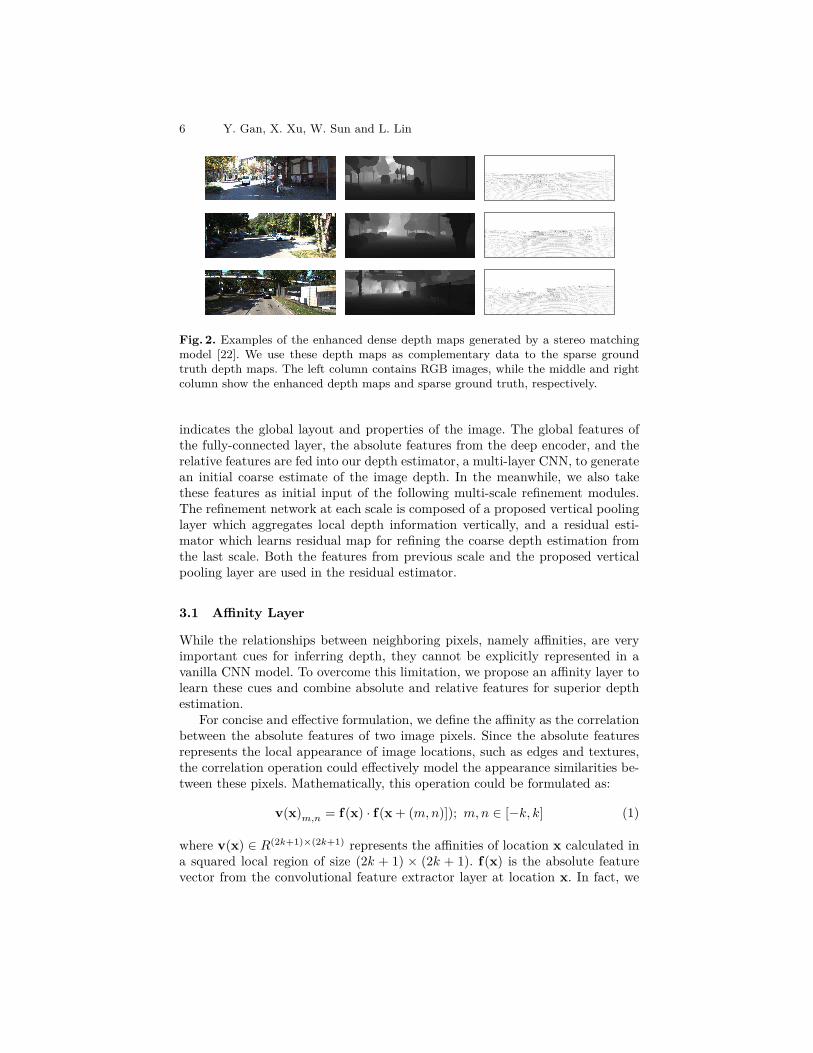
Fig. 2. Examples of the enhanced dense depth maps generated by a stereo matchingmodel [22]. We use these depth maps as complementary data to the sparse groundtruth depth maps. The left column contains RGB images, while the middle and rightcolumn show the enhanced depth maps and sparse ground truth, respectively.

indicates the global layout and properties of the image. The global features ofthe fully-connected layer, the absolute features from the deep encoder, and therelative features are fed into our depth estimator, a multi-layer CNN, to generatean initial coarse estimate of the image depth. In the meanwhile, we also takethese features as initial input of the following multi-scale reinement modules.The reinement network at each scale is composed of a proposed vertical poolinglayer which aggregates local depth information vertically, and a residual esti-mator which learns residual map for reining the coarse depth estimation fromthe last scale. Both the features from previous scale and the proposed verticalpooling layer are used in the residual estimator.

3.1 Ainity Layer

While the relationships between neighboring pixels, namely ainities, are veryimportant cues for inferring depth, they cannot be explicitly represented in avanilla CNN model. To overcome this limitation, we propose an ainity layer tolearn these cues and combine absolute and relative features for superior depthestimation.

For concise and efective formulation, we deine the ainity as the correlationbetween the absolute features of two image pixels. Since the absolute featuresrepresents the local appearance of image locations, such as edges and textures,the correlation operation could efectively model the appearance similarities be-tween these pixels. Mathematically, this operation could be formulated as:

v(x)m,n = f(x) · f(x+ (m,n)]); m,n ∈ [−k, k] (1)

where v(x) ∈ R(2k+1)×(2k+1) represents the ainities of location x calculated ina squared local region of size (2k + 1) × (2k + 1). f(x) is the absolute featurevector from the convolutional feature extractor layer at location x. In fact, we


can reshape v(x) into a 1-dimensional vector of size 1×(2k+1)2, and the relativefeatures of a input image become (2k+1)2 feature maps which could be fed intothe following estimation and reinement layers. Suppose the input feature map isof size w×h×c where w, h and c are the width, height and channels, respectively.w×h×c×(2k+1)2 multiplications are needed for computing the relative featurewhich is computationally heavy. To remedy the problem of the square complexityof the ainity operation, we only perform this layer on the lowest feature scale (inthe context network in Figure 1) to reduce the computational load. The proposedainity layer is integrated in the CNN model and works complementarily withthe absolute features, which signiicantly helps depth estimation.

3.2 Task Speciic Vertical Pooling

Depth distribution in real world scenarios has a special kind of pattern thatthe majority of depth changes lies in the vertical direction. e.g. The road oftenstretches to the far side alone the vertical direction. The faraway objects, suchas sky and mountains, are more likely to be located at the top of a landscapepicture. Recognizing this kind of patterns can provide useful information foraccurate single image depth estimation. However, due to the lack of supervisionand huge parameters space, normal operations in deep neural network such asconvolution and pooling with squared ilters may not be efective in inding suchpatterns. Furthermore, a relative large squared pooling layer aggregates too muchunnecessary information from horizontal locations while it is more eicient toconsider vertical features only.

In this paper, we propose to obtain the local context in vertical directionthrough vertical pooling layer. The vertical pooling layer uses average poolingwith kernels of size H × 1 and outputs feature maps of equal size with the inputfeatures. Multiple vertical pooling layers with diferent kernel heights are usedin our network to handle feature maps across diferent scales. Speciically, weuse four kernels of size 5 × 1, 7 × 1, 11 × 1 and 11 × 1 to process feature mapsof scale S/8, S/4, S/2 and S, where S denotes the resolution of input images.More detailed analysis of vertically aggregating depth information are presentedin Section 4.5.

3.3 Multi-Scale Learning

As shown in Figure 1, our model predicts a coarse depth map through a con-text network. Besides exploiting local context using operations mentioned in thepreview sections, we follow [7] to take advantage of fully connected layers tointegrate a global understanding of the full scene into our network. The outputfeature maps of the encoder and the self-correlation layer are taken as inputof the fully connected layer. The output feature vector of fully connected layeris then reshaped to produce the inal output feature map which is at the 1/8-resolution compared to the input image.

Given the coarse depth map, our model learns to reine the coarse depth byadopting the residual learning scheme propose by He et al. [13]. The reinement


module irst up-sample the input feature map by factor of 2. A residual estimatorthen learns to predict the corresponding residual signal based on the up-sampledfeature, the local context feature and the long skip connected low level feature.Without the need to predict absolute depth values, the reinement module canfocus on learning residual that helps produce accurate depth maps. Such learningstrategy can lead to smaller network and better convergence. Several reinementmodules are employed in our model to produce residuals across multiple scales.The reinement process can be formulated as:

ds = UPds+1+ rs 0 ≤ s ≤ S (2)

where ds and rs denote depth and residual maps that are downsampled by afactor of 2s from full resolution size. UP· denotes 2× upsample operation.We supervise the estimated depth map across S + 1 scales. Ablation study inSection 4.5 demonstrates that incorporating residual learning can lead to moreaccurate depth maps compared to direct learning strategy.

3.4 Loss Function

Ground truth enhancement. The ground truth depth maps obtained fromLidar sensor are too sparse (only 5% pixels are valid) to provide enough super-visory signal for training a deep model. In order to produce high quality, densedepth maps, we enhance the sparse ground truth with dense depth maps pre-dicted by a stereo matching approach [22]. We use both the dense depth mapsand the sparse velodyne data as ground truth at training time. Some samples ofpredicted depth maps are shown in Fig 2.Training loss. The enhanced dense depth maps produced by stereo matchingmodel are not accurate enough compared to ground truth depth maps. The errorbetween predicted and ground truth depth maps is shown in Table 1. We usea weighted sum L2 loss to suppress the noise contained in the enhanced densedepth maps:

Loss =∑

i∈Λ

∥predi − gti∥22 + α ∗

∑

i∈Ω

∥predi − gti∥22 (3)

where predi and gti denote the predicted depth and ground truth depth at ithpixel. Λ denotes a collection of pixels where sparse ground truth values are valid.Ω denotes a collection of pixels where sparse ground truth values are invalid andvalues from enhance depth maps are used as ground truth. α is set to 0.3 in allthe experiments.

4 Experiments

We show the main results in this section and present more evaluations in thesupplementary material.


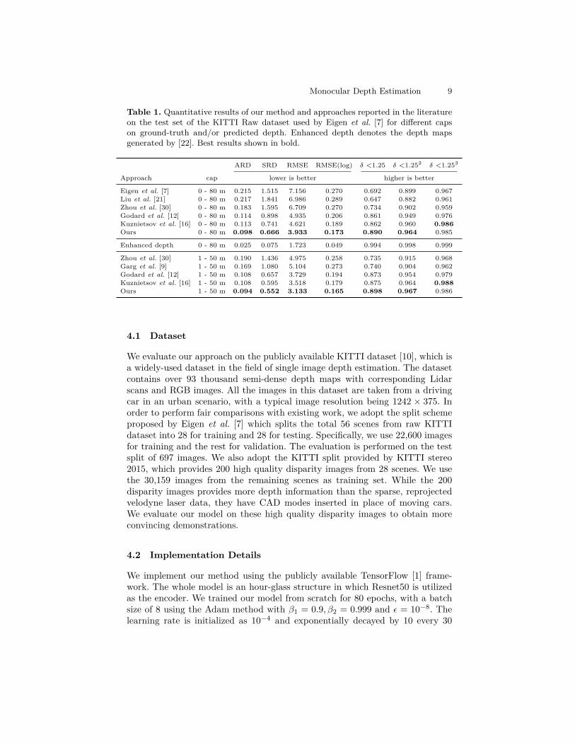
Table 1. Quantitative results of our method and approaches reported in the literatureon the test set of the KITTI Raw dataset used by Eigen et al. [7] for diferent capson ground-truth and/or predicted depth. Enhanced depth denotes the depth mapsgenerated by [22]. Best results shown in bold.

ARD SRD RMSE RMSE(log) δ <1.25 δ <1.252 δ <1.253

Approach cap lower is better higher is better

Eigen et al. [7] 0 - 80 m 0.215 1.515 7.156 0.270 0.692 0.899 0.967Liu et al. [21] 0 - 80 m 0.217 1.841 6.986 0.289 0.647 0.882 0.961Zhou et al. [30] 0 - 80 m 0.183 1.595 6.709 0.270 0.734 0.902 0.959Godard et al. [12] 0 - 80 m 0.114 0.898 4.935 0.206 0.861 0.949 0.976Kuznietsov et al. [16] 0 - 80 m 0.113 0.741 4.621 0.189 0.862 0.960 0.986Ours 0 - 80 m 0.098 0.666 3.933 0.173 0.890 0.964 0.985

Enhanced depth 0 - 80 m 0.025 0.075 1.723 0.049 0.994 0.998 0.999

Zhou et al. [30] 1 - 50 m 0.190 1.436 4.975 0.258 0.735 0.915 0.968Garg et al. [9] 1 - 50 m 0.169 1.080 5.104 0.273 0.740 0.904 0.962Godard et al. [12] 1 - 50 m 0.108 0.657 3.729 0.194 0.873 0.954 0.979Kuznietsov et al. [16] 1 - 50 m 0.108 0.595 3.518 0.179 0.875 0.964 0.988Ours 1 - 50 m 0.094 0.552 3.133 0.165 0.898 0.967 0.986

4.1 Dataset

We evaluate our approach on the publicly available KITTI dataset [10], which isa widely-used dataset in the ield of single image depth estimation. The datasetcontains over 93 thousand semi-dense depth maps with corresponding Lidarscans and RGB images. All the images in this dataset are taken from a drivingcar in an urban scenario, with a typical image resolution being 1242 × 375. Inorder to perform fair comparisons with existing work, we adopt the split schemeproposed by Eigen et al. [7] which splits the total 56 scenes from raw KITTIdataset into 28 for training and 28 for testing. Speciically, we use 22,600 imagesfor training and the rest for validation. The evaluation is performed on the testsplit of 697 images. We also adopt the KITTI split provided by KITTI stereo2015, which provides 200 high quality disparity images from 28 scenes. We usethe 30,159 images from the remaining scenes as training set. While the 200disparity images provides more depth information than the sparse, reprojectedvelodyne laser data, they have CAD modes inserted in place of moving cars.We evaluate our model on these high quality disparity images to obtain moreconvincing demonstrations.

4.2 Implementation Details

We implement our method using the publicly available TensorFlow [1] frame-work. The whole model is an hour-glass structure in which Resnet50 is utilizedas the encoder. We trained our model from scratch for 80 epochs, with a batchsize of 8 using the Adam method with β1 = 0.9, β2 = 0.999 and ϵ = 10−8. Thelearning rate is initialized as 10−4 and exponentially decayed by 10 every 30


epochs during training. All the parameters in our model are initialized basedon xavier algorithm [11]. It costs about 7G of GPU memory and 50 hours totrain our model on a single NVIDIA GeForce GTX TITAN X GPU with 12GBmemory. The average training time for each image is less than 100 ms and ittakes less than 70 ms to test one image.

Data augmentation is also conducted during training process. The input im-age is lipped with a probability of 0.5. We randomly crop the original image intosize of 2h× h to retain image ratio, where h is the height of the original image.The input image is obtained by resizing the cropped image to a resolution of512 × 256. We also performed random brightness for color augmentation, with50% chance, by sampling from a uniform distribution in the range of [0.5, 2.0].

4.3 Evaluation Metrics

We evaluate the performance of our approach in monocular depth predictionusing the velodyne ground truth data on the test images. We follow the depthevaluation metrics used by Eigen et al. [7]:

ARD: 1

|T |

∑

y∈T|y − y∗|/y∗ RMSE:

√

1

|T |

∑

y∈T∥y − y∗∥2

SRD: 1

|T |

∑

y∈T∥y − y∗∥2/y∗ RMSE(log):

√

1

|T |

∑

y∈T∥logy − logy∗∥2

Threshold: % of yi s.t. max( yiy∗ ,

y∗

yi) = δ < thr

where T denotes a collection of pixels where the ground truth values arevalid. y∗ denotes the ground truth value.

4.4 Comparisons with state-of-the-art methods

Table 1 shows the quantitative comparisons between our model and other state-of-the-art methods in monocular depth estimation. It can be observed that ourmethod achieves best performances for all evaluation metrics at both 80m and50m caps, except for the accuracy at δ <1.253 where we obtain comparableresults with Kuznietsov et al. [16] at cap of 80m (0.985 vs 0.986) and 50m (0.986vs 0.988). Speciically, our method reduces the RMSE metric by 20.3% comparedwith Godard et al. [12] and 14.9% compared with Kuznietsov et al. [16] at thecap of 80 m. Furthermore, our model obtain accuracy of 89.0% and 89.8% at δ<1.252 metric at the cap of 80 m and 50 m, outperforming Kuznietsov et al. [16]by 2.8% and 2.4% respectively.

To further evaluate the performance of our approach, we train a variant modelon the training set of the oicial KITTI split and perform evaluation on theKITTI 2015 stereo training set which contains 200 high quality disparity images.We convert these disparity images into depth maps for evaluation using thecamera parameters provided by KITTI dataset. The result is shown in Table 3.


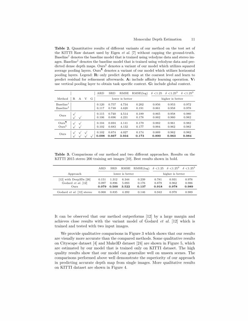
Table 2. Quantitative results of diferent variants of our method on the test set ofthe KITTI Raw dataset used by Eigen et al. [7] without capping the ground-truth.Baseline† denotes the baseline model that is trained using velodyne data and stereo im-ages. Baseline‡ denotes the baseline model that is trained using velodyne data and pre-dicted dense depth maps. Ours§ denotes a variant of our model which utilizes squaredaverage pooling layers. Ours¶ denotes a variant of our model which utilizes horizontalpooling layers. Legend: R: only predict depth map at the coarsest level and learn topredict residual for reinement afterwards. A: include ainity learning operation. V:use vertical pooling layer to obtain task speciic context. G: include global context.


Method R A V G lower is better higher is better

Baseline† 0.120 0.757 4.734 0.202 0.856 0.953 0.972Baseline‡ 0.117 0.748 4.620 0.191 0.861 0.958 0.978

Ours√ 0.115 0.740 4.514 0.189 0.865 0.958 0.980√ √ 0.106 0.696 4.231 0.178 0.882 0.960 0.982

Ours¶ √ √ 0.104 0.694 4.141 0.179 0.882 0.961 0.982Ours§ √ √ 0.102 0.683 4.132 0.177 0.884 0.962 0.982

Ours√ √ √ 0.102 0.674 4.027 0.174 0.889 0.962 0.982√ √ √ √ 0.098 0.667 3.934 0.173 0.890 0.963 0.984

Table 3. Comparisons of our method and two diferent approaches. Results on theKITTI 2015 stereo 200 training set images [10]. Best results shown in bold.


Approach lower is better higher is better

[12] with Deep3Ds [26] 0.151 1.312 6.344 0.239 0.781 0.931 0.976Godard et al. [12] 0.097 0.896 5.093 0.176 0.879 0.962 0.986

Ours 0.079 0.500 3.522 0.137 0.918 0.978 0.989

Godard et al. [12] stereo 0.068 0.835 4.392 0.146 0.942 0.978 0.989

It can be observed that our method outperforms [12] by a large margin andachieves close results with the variant model of Godard et al. [12] which istrained and tested with two input images.

We provide qualitative comparisons in Figure 3 which shows that our resultsare visually more accurate than the compared methods. Some qualitative resultson Cityscape dataset [4] and Make3D dataset [24] are shown in Figure 5, whichare estimated by our model that is trained only on KITTI dataset. The highquality results show that our model can generalize well on unseen scenes. Thecomparisons performed above well demonstrate the superiority of our approachin predicting accurate depth map from single images. More qualitative resultson KITTI dataset are shown in Figure 4.


Fig. 3. Qualitative results on the test set of the KITTI Raw dataset used by Eigen etal. [7]. From top to bottom, the images are input, ground truth, results of Eigen et al.[7], results of Garg et al. [9], results of Godard et al. [12] and results of our method,respectively. Sparse ground truth have been interpolated for better visualization.

4.5 Ablation study

In this subsection, we show efectiveness and necessity of each component in ourproposed model and also demonstrate the efectiveness of the network design.Supervisory signal: To validate the efectiveness of using predicted densedepth maps as ground truth at training time. We compare our baseline model(denoted as Baseline‡) with a variant (denoted as Baseline†) which is trained us-ing image alignment loss. Results are shown in the irst two rows of Table 2. It canbe easily observed that Baseline‡ achieves better results than Baseline† on all themetrics. This may due to the well known fact that stereo depth reconstructionbased on image matching is an ill-pose problem. Training on a image alignmentloss may provide inaccurate supervisory signal. On the contrary, the dense depthmaps used in our method are more accurate and more robust against the ambi-guity, since they are produced by a powerful stereo matching model [22] whichis well designed and trained on massive data for the task of depth reconstruc-tion. Thus, the superior result, together with the above analysis, well validatethat utilizing predicted depth maps as ground truth can provide more usefulsupervisory signal.Residual learning vs direct learning: The baseline model of our approach(denoted as Baseline‡) is implemented using direct learning strategy which learnsto output the depth map directly instead of the residual depth map. Note thatthe baseline model represents our network without any of the components R,A, V, G in Table 2. As shown in Table 2, the baseline model achieves 0.117 atARD metric and 4.620 at RMSE metric. In order to compare residual learningstrategy with direct learning strategy, we replace direct learning with residuallearning in Baseline‡ and keep other settings identical to obtain a variant model


Table 4. Quantitative results on NYU Depth v2 dataset(part). H-pooling denoteshorizontal pooling. Note that our model was trained on the labeled training set with795 images instead of the full dataset which contains 20K images.

Method δ <1.25 δ <1.252 δ <1.253 rel log10 rms

w/ H-pooling 0.747 0.929 0.977 0.165 0.069 0.652w/o ainity 0.732 0.920 0.972 0.179 0.075 0.694

Ours 0.756 0.934 0.980 0.158 0.066 0.631

Fig. 4. More qualitative results on KITTI test splits.

with residual learning strategy. The performance of this variant model is shownin the third row of Table 2, which outperforms Baseline‡ with slight improve-ments on all the metrics. This may due the reason that residual learning canfocus on modeling the highly non-linear residuals while direct learning needs topredict absolute depth values. Moreover, residual learning also helps alleviatethe problem of over-itting [13].Pooling methods: To validate the idea that incorporating local context throughpooling layers helps boost the performance of depth estimation, we implementthree variant models that use vertical pooling layers, horizontal pooling layers(denoted as Ours¶) and squared average pooling layers (denoted as Ours§). Notethat we also use multiple average pooling layers with kernels of diferent sizesto handle multi-scale feature maps. Speciically, we use four squared averagepooling layers in Ours§ whose kernel sizes are set to 5 × 5, 7 × 7, 11 × 11 and11× 11 respectively. The results are shown in the middle three lines of Table 2.As one can see, by adopting squared average pooling layers, the model achievesslightly better results where SRD metric is reduced from 0.696 to 0.683 whileRMSE metric is reduced from 4.231 to 4.132. The improvement demonstrates theefectiveness of exploiting local context through pooling layers. Similar improve-ments can be observed by integrating horizontal pooling layers. Furthermore, byreplacing squared average polling layers with vertical pooling layers, our modelobtains better results with more signiicant improvements. The further improve-ment proves that vertical pooling is able to model the local context more efec-tively compared to squared average pooling and horizontal pooling. This maydue to the reason that squared average pooling combines both the depth distri-bution alone the horizontal and vertical direction which might introduce noiseand redundant information.


Fig. 5. Qualitative results on Make3D dataset [24] (left two columns) and Cityscapedataset [4] (right two columns).

Contribution of each component: To discover the vital elements in our pro-posed method, we conduct ablation study by gradually integrating each compo-nent into our model. The results are shown in Table 2. Besides the improvementsbrought by residual learning and vertical pooling modules which have been an-alyzed in the above comparisons, integrating ainity layer can result in majorimprovements on all the metrics. This proves that ainity layer is the key compo-nent of our proposed approach and thus well validate the insight that explicitlyconsidering relative features between neighboring patches can help the monoc-ular depth estimation. Moreover, integrating fully connected layers to exploitglobal context information further boosts the performance of our model. It canbe seen from the last row of Table 2 that accuracy at δ <1.253 is further im-proved to 0.984. This shows that some challenge outliers can be predicted moreaccurately given the global context information.

We conduct more experiments to evaluate the proposed components on theNYUv2 dataset in Table 4. The Results further prove that ainity layer andvertical pooling both play an important role in improving the estimation perfor-mance, which also shows that proposed method generalizes well to the NYUv2dataset.

5 Conclusions

In this work, we propose a novel ainity layer to model the relationship betweenneighboring pixels, and integrate this layer into CNN to combine absolute andrelative features for depth estimation. In addition, we exploit the prior knowl-edge that vertical information potentially helps depth inference and develop ver-tical pooling to aggregate local features. Furthermore, we enhance the originalsparse depth labels by using stereo matching network to generate high-qualitydepth predictions from left-right image pairs to assist the training process. Wealso adopt a multi-scale architecture with residual learning for improved depthestimation. The proposed method performs favorably against the state-of-the-art monocular depth algorithms both qualitatively and quantitatively. In futurework, we will investigate more about the generalization abilities of the ainitylayer and vertical pooling for indoor scenes. It will also be interesting to ex-plore more detailed geometry relations and semantic segmentation informationfor more robust depth estimation.


References

1. Abadi, M., Barham, P., Chen, J., Chen, Z., Davis, A., Dean, J., Devin, M., Ghe-mawat, S., Irving, G., Isard, M., et al.: Tensorlow: A system for large-scale machinelearning. In: OSDI. vol. 16, pp. 265–283 (2016)

2. Cao, Y., Wu, Z., Shen, C.: Estimating depth from monocular images as classi-ication using deep fully convolutional residual networks. IEEE Transactions onCircuits and Systems for Video Technology (2017)

3. Chen, W., Fu, Z., Yang, D., Deng, J.: Single-image depth perception in the wild.In: Advances in Neural Information Processing Systems. pp. 730–738 (2016)

4. Cordts, M., Omran, M., Ramos, S., Rehfeld, T., Enzweiler, M., Benenson, R.,Franke, U., Roth, S., Schiele, B.: The cityscapes dataset for semantic urban sceneunderstanding. In: Proceedings of the IEEE conference on computer vision andpattern recognition. pp. 3213–3223 (2016)

5. Cui, Y., Zhou, F., Wang, J., Liu, X., Lin, Y., Belongie, S.J.: Kernel pooling forconvolutional neural networks. In: CVPR. vol. 1, p. 7 (2017)

6. Eigen, D., Fergus, R.: Predicting depth, surface normals and semantic labels witha common multi-scale convolutional architecture. In: Proceedings of the IEEE In-ternational Conference on Computer Vision. pp. 2650–2658 (2015)

7. Eigen, D., Puhrsch, C., Fergus, R.: Depth map prediction from a single image usinga multi-scale deep network. In: Advances in neural information processing systems.pp. 2366–2374 (2014)

8. Gao, Y., Beijbom, O., Zhang, N., Darrell, T.: Compact bilinear pooling. In: Pro-ceedings of the IEEE conference on computer vision and pattern recognition. pp.317–326 (2016)

9. Garg, R., BG, V.K., Carneiro, G., Reid, I.: Unsupervised cnn for single view depthestimation: Geometry to the rescue. In: European Conference on Computer Vision.pp. 740–756. Springer (2016)

10. Geiger, A., Lenz, P., Urtasun, R.: Are we ready for autonomous driving? the kittivision benchmark suite. In: Computer Vision and Pattern Recognition (CVPR),2012 IEEE Conference on. pp. 3354–3361. IEEE (2012)

11. Glorot, X., Bengio, Y.: Understanding the diiculty of training deep feedforwardneural networks. In: Aistats. vol. 9, pp. 249–256 (2010)

12. Godard, C., Mac Aodha, O., Brostow, G.J.: Unsupervised monocular depth esti-mation with left-right consistency. In: CVPR. vol. 2, p. 7 (2017)

13. He, K., Zhang, X., Ren, S., Sun, J.: Deep residual learning for image recognition. In:Proceedings of the IEEE conference on computer vision and pattern recognition.pp. 770–778 (2016)

14. Karsch, K., Liu, C., Kang, S.B.: Depth extraction from video using non-parametricsampling. In: European Conference on Computer Vision. pp. 775–788. Springer(2012)

15. Konrad, J., Wang, M., Ishwar, P.: 2d-to-3d image conversion by learning depth fromexamples. In: Computer Vision and Pattern Recognition Workshops (CVPRW),2012 IEEE Computer Society Conference on. pp. 16–22. IEEE (2012)

16. Kuznietsov, Y., Stückler, J., Leibe, B.: Semi-supervised deep learning for monoc-ular depth map prediction. In: Proc. of the IEEE Conference on Computer Visionand Pattern Recognition. pp. 6647–6655 (2017)

17. Ladicky, L., Shi, J., Pollefeys, M.: Pulling things out of perspective. In: Proceedingsof the IEEE Conference on Computer Vision and Pattern Recognition. pp. 89–96(2014)


18. Li, B., Shen, C., Dai, Y., van den Hengel, A., He, M.: Depth and surface normalestimation from monocular images using regression on deep features and hierarchi-cal crfs. In: Proceedings of the IEEE Conference on Computer Vision and PatternRecognition. pp. 1119–1127 (2015)

19. Lin, T.Y., RoyChowdhury, A., Maji, S.: Bilinear cnn models for ine-grained visualrecognition. In: Proceedings of the IEEE International Conference on ComputerVision. pp. 1449–1457 (2015)

20. Liu, B., Gould, S., Koller, D.: Single image depth estimation from predicted se-mantic labels. In: Computer Vision and Pattern Recognition (CVPR), 2010 IEEEConference on. pp. 1253–1260. IEEE (2010)

21. Liu, M., Salzmann, M., He, X.: Discrete-continuous depth estimation from a singleimage. In: Computer Vision and Pattern Recognition (CVPR), 2014 IEEE Con-ference on. pp. 716–723. IEEE (2014)

22. Pang, J., Sun, W., Ren, J., Yang, C., Yan, Q.: Cascade residual learning: A two-stage convolutional neural network for stereo matching. In: International Conf. onComputer Vision-Workshop on Geometry Meets Deep Learning (ICCVW 2017).vol. 3 (2017)

23. Saxena, A., Chung, S.H., Ng, A.Y.: Learning depth from single monocular images.In: Advances in neural information processing systems. pp. 1161–1168 (2006)

24. Saxena, A., Sun, M., Ng, A.Y.: Make3d: Learning 3d scene structure from a singlestill image. IEEE transactions on pattern analysis and machine intelligence 31(5),824–840 (2009)

25. Tomasi, C., Manduchi, R.: Bilateral iltering for gray and color images. In: Com-puter Vision, 1998. Sixth International Conference on. pp. 839–846. IEEE (1998)

26. Xie, J., Girshick, R., Farhadi, A.: Deep3d: Fully automatic 2d-to-3d video conver-sion with deep convolutional neural networks. In: European Conference on Com-puter Vision. pp. 842–857. Springer (2016)

27. Xu, D., Ricci, E., Ouyang, W., Wang, X., Sebe, N.: Multi-scale continuous crfsas sequential deep networks for monocular depth estimation. In: Proceedings ofCVPR. vol. 1 (2017)

28. Xu, X., Pan, J., Zhang, Y.J., Yang, M.H.: Motion blur kernel estimation via deeplearning. TIP 27, 194–205 (2018)

29. Xu, X., Sun, D., Pan, J., Zhang, Y., Pister, H., Yang, M.H.: Learning to super-resolve blurry face and text images. In: ICCV (2017)

30. Zhou, T., Brown, M., Snavely, N., Lowe, D.G.: Unsupervised learning of depth andego-motion from video. In: CVPR. vol. 2, p. 7 (2017)

monocular depth estimation with affinity, vertical pooling, and label...

Documents