monopoly power and endogenous product variety: distortions

American Economic Journal: Macroeconomics 2019, 11(4): 140–174 https://doi.org/10.1257/mac.20170303

140

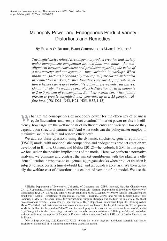
Monopoly Power and Endogenous Product Variety: Distortions and Remedies†

By Florin O. Bilbiie, Fabio Ghironi, and Marc J. Melitz*

The inefficiencies related to endogenous product creation and variety under monopolistic competition are two-fold: one static—the mis-alignment between consumers and producers regarding the value of a new variety; and one dynamic—time variation in markups. When production factors (labor and physical capital ) are elastic and traded in competitive markets, further distortions appear. Appropriate taxa-tion schemes can restore optimality if they preserve entry incentives. Quantitatively, the welfare costs of each distortion by itself amounts to 2 to 5 percent of consumption. But their overall cost when jointly present is greatly magnified, and generates up to a 25 percent wel-fare loss. (JEL D21, D43, H21, H25, H32, L13)

What are the consequences of monopoly power for the efficiency of business cycle fluctuations and new product creation? If market power results in ineffi-

ciency, how large are the welfare costs of inefficient entry and variety? How do they depend upon structural parameters? And what tools can the policymaker employ to maximize social welfare and restore efficiency?

We address these questions using the dynamic, stochastic, general equilibrium (DSGE) model with monopolistic competition and endogenous product creation we developed in Bilbiie, Ghironi, and Melitz (2012)—henceforth, BGM. In that paper, we focused on the positive implications of the model. Here, we perform a normative analysis: we compare and contrast the market equilibrium with the planner’s effi-cient allocation in response to exogenous aggregate shocks when product creation is subject to sunk costs, a time-to-build lag, and an obsolescence risk. We then quan-tify the welfare cost of distortions in a calibrated version of the model. We use the

* Bilbiie: Department of Economics, University of Lausanne and CEPR; Internef, Quartier Chamberonne, CH-1015 Lausanne, Switzerland (email: [email protected]); Ghironi: Department of Economics, University of Washington, EABCN, CEPR, and NBER; Savery Hall, Box 353330, Seattle, WA 98195 (email: [email protected]); Melitz: Department of Economics, Harvard University, CEPR, and NBER; Littauer Center 215, Cambridge, MA 02138 (email: [email protected]). Virgiliu Midrigan was coeditor for this article. We thank two anonymous referees, Sanjay Chugh, Ippei Fujiwara, Hugo Hopenhayn, Giammario Impullitti, Henning Weber, Mirko Wiederholt, and participants in numerous seminars and conferences for helpful comments. We are grateful to Michel Juillard for help and to Pablo Winant for developing the first code to solve our nonlinear model, and to Ezgi Ozsogut for further developing that code and superb research assistance. Bilbiie gratefully acknowledges without implicating the support of Banque de France via the eponymous Chair at PSE, and of Institut Universitaire de France.

† Go to https://doi.org/10.1257/mac.20170303 to visit the article page for additional materials and author disclosure statement(s) or to comment in the online discussion forum.

https://doi.org/10.1257/mac.20170303

mailto:[email protected]




https://doi.org/10.1257/mac.20170303

VOL. 11 NO. 4 141BILBIIE ET AL.: MONOPOLY, ENTRY, AND VARIETY: DISTORTIONS AND REMEDIES

same calibrated parameters as BGM, which best match the US business cycle data, on entry, product creation, and the cyclicality of profits and markups. Lastly, we describe some fiscal policies that ensure implementation of the Pareto optimum as a market equilibrium when efficiency of the market solution fails. The policy schemes that implement efficiency in our model fully specify the optimal path of the relevant instruments over the business cycle.1

Our main theorem identifies two distortions as the sources of inefficient entry and product variety under general preferences over consumption varieties. The first dis-tortion, which we label “static,” pertains to the intra-temporal misalignment between the benefit of an extra variety to the consumer and the profit incentive for an entrant to produce that extra variety. The second distortion, which we label “dynamic,” is associated with the inter-temporal variation of markups. Both distortions disappear if and only if preferences are of the C.E.S. form originally studied by Dixit and Stiglitz (1977)—in which case our dynamic market equilibrium is also efficient.

The policymaker can use a variety of fiscal instruments (in conjunction with lump-sum taxes or transfers) to alleviate these distortions and ensure implementa-tion of the first-best equilibrium. We study an example consisting of a combination of appropriately designed taxes on consumption and dividends (equal to profits in our model) that can implement the first-best equilibrium. The dividend tax aligns firms’ entry incentives with consumers’ love for variety, while the consumption tax corrects for the inefficient allocation of resources that is due to the inter-temporal misalignment of markups.

Efficiency also requires that markups be synchronized across all items that bring utility (or disutility) to consumers.2 When labor supply is endogenous, a new lei-sure good is introduced that is not subject to markup pricing. This opens a wedge between marginal rates of substitution and transformation between consumption and leisure that distorts labor supply. We analyze this case separately and show how efficiency is restored if the government taxes leisure (or subsidizes labor supply) at a rate equal to the net markup in consumption goods prices (even though goods are priced above marginal cost). While this result also holds in a model with a fixed number of firms, an equivalent optimal policy in that setup would have the markup removed by a proportional revenue subsidy. In our model, such a policy of inducing marginal cost pricing—if financed with lump-sum taxation of firm profits—would eliminate entry incentives, since the sunk entry cost could not be covered in the

1 By studying the efficiency properties of our model, this paper contributes to the literature on the efficiency properties of monopolistic competition started by the original work of Lerner (1934) and developed by Samuelson (1947), Spence (1976), Dixit and Stiglitz (1977), and Grossman and Helpman (1991), among others. See also Mankiw and Whinston (1986); Benassy (1996); Kim (2004); and Opp, Parlour, and Walden (2014).

2 The point that efficiency occurs with synchronized markups can be traced back to Lerner (1934) and Samuelson (1947). Lerner (1934, 172) first noted that the allocation of resources is efficient when markups are equal in the pricing of all goods: “The conditions for that optimum distribution of resources between different commodities that we designate the absence of monopoly are satisfied if prices are all proportional to marginal cost.” Samuelson (1947, 239–40) also makes this point clearly: “If all factors of production were indifferent between different uses and completely fixed in amount—the pure Austrian case—, then [ … ] proportionality of prices and marginal cost would be sufficient.” This makes it clear that equality of prices to marginal cost is not necessary for achieving an optimal allocation, contrary to an argument often found in the macroeconomic policy literature. This point is equally true in a model with a fixed number of firms, where the planner merely solves a static allocation problem, allocating labor to the symmetric individual goods evenly.

142 AMERICAN ECONOMIC JOURNAL: MACROECONOMICS OCTOBER 2019

absence of profits.3 These results highlight the importance of preserving the optimal (from the standpoint of generating the welfare-maximizing level of product variety) amount of monopoly profits in economies in which firm entry is costly. Our findings thus caution against interpretations of statements in the recent literature on the “dis-tortionary” consequences of monopoly power and on the required remedies.4

When investment in physical capital is endogenous, a different inefficiency wedge arises due to monopoly power in the goods market: intangible investment in new goods yields a higher rate of return than investment in this latter type of tangi-ble (physical) capital. This leads to underinvestment in this latter type of tangible capital in the market equilibrium, and suboptimal production of the consumption good. This distortion can be remedied directly by subsidizing physical capital at a rate equal to the net markup, which aligns incentives to invest in the two types of capital.

We quantify the welfare cost of these inefficiencies in a calibrated version of our model based on BGM and find that they are sizable. We find that the static distortion for new goods dominates the dynamic one (markup fluctuations over time). On its own, this static distortion accounts for roughly 2 percent of consumption. The dis-tortions due to elastic factors are also large: 5 percent for elastic labor and 2 percent for endogenous investment (again in terms of consumption). Moreover, we find that the impact of these distortions is magnified when they are jointly present: they then combine to generate a welfare loss of 25 percent—vastly greater than the indepen-dent sum of the individual distortions. We also show that this magnification effect continues to hold even when labor supply is very inelastic, and the individual labor distortion is low.

Our findings point to the paramount importance of empirical investigation of (an aggregate measure of) the love for variety, in particular in relationship with mark-ups, as key determinants of the welfare properties of models with entry, variety, and endogenous markups.

The framework and results developed herein provide the foundation for a number of applications and extensions that have appeared in subsequent normative analy-ses of different policies in macroeconomic models.5 One other important distortion addressed by the literature arises with the introduction of producer heterogeneity.

3 We are implicitly assuming that the government is not contemporaneously subsidizing the entire amount of the entry cost. When labor supply is endogenous, we show that inducing marginal cost pricing can implement the efficient equilibrium in our model only when the lump-sum taxation that finances the necessary sales subsidy is optimally split between households and firms, and that this requires zero lump-sum taxation of firm profits when preferences are of the form studied by Dixit and Stiglitz (1977).

4 In particular, our results stand in sharp contrast to the common policy prescription of eliminating monopoly profits, found in a large body of literature studying optimal monetary and fiscal policy in the presence of monopo-listic competition.

5 To give some examples, Bilbiie, Ghironi, and Melitz (2008) relies on results in this paper when discussing optimal monetary policy in a sticky-price version of the model in which policy can deliver the first-best outcome. Bilbiie, Fujiwara, and Ghironi (2014) studies Ramsey-optimal monetary policy in a second-best environment. Bergin and Corsetti (2008, 2014); Cacciatore, Fiori, and Ghironi (2016); Cacciatore and Ghironi (2012); Cooke (2016); Etro and Rossi (2015); Faia (2012); and Lewis (2013) also build on the framework and insights herein—or use related frameworks—to study optimal monetary policy. Chugh and Ghironi (2018) uses our model to study Ramsey-optimal fiscal policy, while Colciago and Etro (2010), Lewis and Winkler (2015), and Colciago (2016) focus on the consequences of oligopolistic competition and Bertoletti and Etro (2016) and Etro (2016) on environ-ments with non-homothetic preferences.


This generates a different static distortion due to the misalignment of markups across producers. Epifani and Gancia (2011) studies misallocation resulting from heterogenous markups across sectors and its consequences for the welfare effects of trade liberalization. Dhingra and Morrow (2019) extends the normative analysis of Dixit and Stiglitz (1977) to the case of firm heterogeneity under general additively separable preferences with variable elasticities of substitution (this is the monopo-listic competition equilibrium studied by Zhelodboko et al. 2012).

More recently, Edmond, Midrigan, and Xu (2018) calibrates a dynamic model with producer heterogeneity and endogenous markups (over time and across pro-ducers) and quantify the welfare distortions associated with those markups and entry. Like us, they find that this impact is substantial (7.5 percent for their baseline calibration). Baqaee and Farhi (2018) focus exclusively on misallocation across het-erogeneous producers: in their model with calibrated firm-level markups, the cost of such distortions amounts to 20 percent in aggregate TFP units. Acemoglu et al. (2018) examines distortions associated with a different type of cross-firm heteroge-neity relating to R&D potential. In this case, distortions arise due to the misallocation of R&D resources across firms. In this paper, we abstract from these other sources of distortions in order to focus on the static and dynamic ones associated with endoge-nous entry and product variety and their interaction with elastic production factors.

The structure of the paper is as follows. Section I describes the benchmark model with fixed labor supply and characterizes the market equilibrium and (in subsec-tion IF) the Pareto-optimal allocation of the social planner. Section II states and proves our welfare theorem, and discusses the intuition behind it. Section III extends our model to elastic factors of production (both labor and physical capital). Section IV describes our calibration of the model to fit key US business cycle moments and quantifies the welfare distortions. Section V concludes.

I. A Model of Endogenous Entry and Product Variety

This section outlines the model and solves for the monopolistically competitive market equilibrium and for the Pareto-optimal planner equilibrium, respectively.

A. Household Preferences

The economy is populated by a unit mass of atomistic households. We begin by assuming that the representative household supplies L units of labor inelastically in each period at the nominal wage rate W t (and extend this to endogenous labor below). The household maximizes expected inter-temporal utility from consumption ( C ): E t ∑ s=t

∞ β s−t U( C s ) , where β ∈ (0, 1) is the subjective discount factor and U(C) is a period utility function with the standard properties. At time t , the household con-sumes the basket of goods C t , defined as a homothetic aggregate over a continuum of goods Ω . At any given time t , only a subset of goods Ω t ⊂ Ω is available. Let p t (ω) denote the nominal price of a good ω ∈ Ω t . Our model can be solved for any parametrization of symmetric homothetic preferences. For any such preferences, there exists a well defined homothetic consumption index C t and an associated welfare-based price index P t . The demand for an individual variety, c t (ω) , is then


obtained as c t (ω)dω = C t ∂ P t /∂ p t (ω) , where we use the conventional notation for quantities with a continuum of goods as flow values.6

Given the demand for an individual variety, c t (ω) , the symmetric price elasticity of demand is in general a function of the number N t of goods/producers (where N t is the mass of Ω t , and θ measures the elasticity of substitution):

θ ( N t ) ≡ − ∂ c t (ω)

_ ∂ p t (ω) p t (ω)

_ c t (ω)

, for any symmetric variety ω.

The welfare gain of additional product variety is captured by the relative price ρ :

ρ t (ω) = ρ ( N t ) ≡ p t (ω)

_ P t , for any symmetric variety ω,

or, in elasticity form:

ϵ ( N t ) ≡ ρ′ ( N t )

_____ ρ ( N t ) N t .

Together, θ( N t ) and ρ( N t ) completely characterize the choice of symmetric homo-thetic preferences in our model; explicit expressions can be obtained for these objects upon specifying functional forms for preferences, as will become clear in the discussion below.

B. Firms

There is a continuum of monopolistically competitive firms, each producing a different variety ω ∈ Ω . Production requires only one factor, labor. Aggregate labor productivity is indexed by Z t , which represents the effectiveness of one unit of labor; Z t is exogenous and follows an AR(1) process (in logarithms). Output supplied by firm ω is y t (ω) = Z t l t (ω) , where l t (ω) is the firm’s labor demand for productive purposes. The unit cost of production, in units of the consumption good C t , is w t / Z t , where w t ≡ W t / P t is the real wage.7

Prior to entry, firms face a sunk entry cost of f E effective labor units, equal to w t f E / Z t units of the consumption basket. There are no fixed production costs. Hence, all firms that enter the economy produce in every period, until they are hit with a “death” shock, which occurs with probability δ ∈ (0, 1) in every period.8

Given our modeling assumption relating each firm to an individual variety, we think of a firm as a production line for that variety, and the entry cost as the develop-ment and setup cost associated with the latter (potentially influenced by market reg-ulation). The exogenous “death” shock also takes place at the individual variety level. Empirically, a firm may comprise more than one of these production lines, but—for

6 See the Appendix for more details. Since this is a real model, the nominal price of the consumption basket is not determined; we use the consumption basket as the numeraire.

7 Consistent with standard real business cycle theory, aggregate productivity Z t affects all firms uniformly.8 For simplicity, we do not consider endogenous exit. As we show in BGM, appropriate calibration of δ makes

it possible for our model to match several important features of the data.


simplicity—our model does not address the determination of product variety within firms.

Firms set prices in a flexible fashion as markups over marginal costs. In units of consumption, firm ω ’s price is ρ t (ω) = μ t w t / Z t , where the markup μ t is in gen-eral a function of the number of producers: μ t = μ( N t ) ≡ θ (N t )/(θ( N t ) − 1). The firm’s profit in units of consumption, returned to households as dividend, is d t (ω) = (1 − μ ( N t ) −1 ) Y t

C / N t , where Y t C is total output of the consumption basket and

will in equilibrium be equal to total consumption demand C t .

Preference Specifications and Markups.—We consider four alternative pref-erence specifications with symmetric varieties as special cases for illustrative purposes below. The first preference specification features a constant elastic-ity of substitution between goods as in Dixit and Stiglitz (1977). For these C.E.S. preferences (henceforth, C.E.S.-DS), the consumption aggregator is C t = ( ∫ ω∈Ω

c t (ω) (θ−1)/θ dω ) θ/(θ−1) , where θ > 1 is the symmetric elastic-

ity of substitution across goods. The consumption-based price index is then P t = ( ∫ ω∈ Ω t

p t (ω) 1−θ dω) 1/(1−θ) , and the household’s demand for each individual good

ω is c t (ω) = ( p t (ω)/ P t ) −θ C t . It follows that the markup and the benefit of variety are independent of the number of goods: μ( N t ) − 1 = ϵ( N t ) = ϵ = 1/(θ − 1) . The second specification, a variant of C.E.S. with generalized love of variety, was introduced by the working paper version of Dixit and Stiglitz (1977) and used also by Benassy (1996). This variant disentangles monopoly power (measured by the net markup 1/(θ − 1) ) and consumer love for variety, captured by a constant parameter ξ > 0 . With this specification (labeled “general C.E.S.” henceforth), the consump-tion basket is C t = (N t ) ξ− 1 _ θ−1

( ∫ ω∈Ω c t (ω) (θ−1)/θ dω ) θ/(θ−1) . The third preference

specification uses the translog expenditure function proposed by Feenstra (2003). For this specification, the symmetric price elasticity of demand is θ( N t ) = 1 + σ N t , where σ > 0 is a free parameter. The expression for relative price ρ( N t ) is given in Table 1. For translog preferences, N ̃ ≡ mass(Ω) ≥ N t represents the number of all potentially available varieties and is invariant over time. As the number of goods consumed N t increases, goods become closer substitutes, and the elasticity of substi-tution increases. If goods are closer substitutes, then both the markup μ( N t ) and the benefit of additional varieties in elasticity form ( ϵ( N t ) ) must decrease;9 for this spe-cific functional form, the change in ϵ( N t ) is only half the change in the net markup generated by an increase in the number of producers. Finally, the fourth preference specification features exponential love-of-variety (henceforth, “exponential”) and is in some sense the opposite of the general C.E.S. specification: the elasticity of sub-stitution is not constant (because of demand-side pricing complementarities), but the benefit of variety is equal to the net markup. Specifically, the symmetric elasticity of substitution is of the same form as under translog θ( N t ) = 1 + α N t , where α > 0 is a free parameter. However, differently from translog, the relative price is given by ρ( N t ) = e − 1 _ α N t

: it follows that the benefit of variety is equal to the markup (and

9 This property for the markup occurs whenever the price elasticity of residual demand decreases with quantity consumed along the residual demand curve.


profit incentive for entry): ϵ( N t ) = μ( N t ) − 1 = 1/α N t . 10 Table 1 summarizes the

expressions for markup, relative price, and benefit of variety in elasticity form for each preference specification. These functions fully characterize preferences in each case. For the case of the general C.E.S. and exponential preferences, we note that this utility representation would be a function of the number of available varieties (the N ̃ for the translog case) in addition to the variety consumption levels c t (ω) .

Firm Entry and Exit.—In every period, there is a mass N t of firms producing in the economy and an unbounded mass of prospective entrants. These entrants are forward looking, and correctly anticipate their expected future profits d s (ω) in every period s ≥ t + 1 as well as the probability δ (in every period) of incurring the exit-inducing shock. Entrants at time t only start producing at time t + 1 , which introduces a one-period time-to-build lag in the model. The exogenous exit shock occurs at the very end of the time period (after production and entry). A proportion δ of new entrants will therefore never produce. Prospective entrants in period t com-pute their expected post-entry value ( v t (ω) ) given by the present discounted value of their expected stream of profits { d s (ω)} s=t+1

∞ :

(1) v t (ω) = E t ∑ s=t+1

∞

[β (1 − δ) ] s−t

U′ ( C s )

______ U′ ( C t )

d s (ω) .

This also represents the value of incumbent firms after production has occurred (since both new entrants and incumbents then face the same probability 1 − δ of survival and production in the subsequent period). Entry occurs until firm value is equalized with the entry cost, leading to the free entry condition v t (ω) = w t f E / Z t . This condition holds so long as the mass N E,t of entrants is positive. We assume that macroeconomic shocks are small enough for this condition to hold in every period.11 Finally, the timing of entry and production is such that the number of pro-ducing firms during period t is given by N t = (1 − δ )( N t−1 + N E,t−1 ) . The number of producing firms represents the capital stock of the economy. It is an endogenous state variable that behaves much like physical capital in a benchmark real business cycle (RBC) model.

10 As we shall see, the exponential specification eliminates entry inefficiency but introduces markup misalign-ment over time, whereas the general C.E.S. specification features inefficient entry but with constant markups. Both distortions operate under translog preferences.

11 Periods with zero entry ( N E,t = 0 ) may occur as a consequence of large enough (adverse) exogenous shocks. In these periods, the free entry condition would hold as a strict inequality: v t (ω) < w t f E / Z t .

Table 1—Four Preference Specifications: Markup, Relative Price, and Benefit of Variety

C.E.S.–DS General C.E.S. Translog Exponential

Markup μ ( N t ) = θ ( N t )

_ θ ( N t ) −1 μ = θ _ θ − 1 μ = θ _ θ − 1 1 + 1 _ σ N t

1 + 1 _ α N t

Relative price ρ ( N t ) N t 1 _ θ−1

N t

ξ e − 1 _ 2 N ̃ − N t _ σ N ̃ N t

e − 1 _ α N t

Benefit of variety ϵ ( N t ) μ − 1 ξ 1 _ 2σ N t =

μ ( N t ) − 1 _ 2 1 _ α N t

= μ ( N t ) − 1


Symmetric Firm Equilibrium.—All firms face the same marginal cost. Hence, equilibrium prices, quantities, and firm values are identical across firms: p t (ω) = p t , ρ t (ω) = ρ t , l t (ω) = l t , y t (ω) = y t , d t (ω) = d t , v t (ω) = v t . In turn, equality of prices across firms implies that the consumption-based price index P t and the firm-level price p t are such that p t / P t ≡ ρ t = ρ( N t ) . An increase in the number of firms is associated with an increase in this relative price: ρ′ ( N t ) > 0 , capturing the love of variety utility gain. The aggregate consumption output of the economy is Y t

C = N t ρ t y t = C t .Importantly, in the symmetric firm equilibrium, the value of waiting to enter is

zero, despite the entry decision being subject to sunk costs and exit risk; i.e., there are no option-value considerations pertaining to the entry decision. This happens because all uncertainty in our model (including the “death” shock) is aggregate.12

C. Household Budget Constraint and Inter-temporal Decisions

We assume without loss of generality that households hold only shares in a mutual fund of firms. Let x t be the share in the mutual fund of firms held by the representative household entering period t . The mutual fund pays a total profit in each period (in units of currency) equal to the total profit of all firms that produce in that period, P t N t d t . During period t , the representative household buys x t+1 shares in a mutual fund of N H,t ≡ N t + N E,t firms (those already operating at time t and the new entrants). Only N t+1 = (1 − δ ) N H,t firms will produce and pay dividends at time t + 1 . Since the household does not know which firms will be hit by the exog-enous exit shock δ at the very end of period t , it finances the continuing operation of all preexisting firms and all new entrants during period t . The date t price (in units of currency) of a claim to the future profit stream of the mutual fund of N H,t firms is equal to the nominal price of claims to future firm profits, P t v t .

The household enters period t with mutual fund share holdings x t and receives dividend income and the value of selling its initial share position, and labor income. The household allocates these resources between purchases of shares to be carried into next period, consumption, and lump-sum taxes T t levied by the government. The period budget constraint (in units of consumption) is

(2) v t N H,t x t+1 + C t = ( d t + v t ) N t x t + w t L.

The household maximizes its expected inter-temporal utility subject to (2). The Euler equation for share holdings is

v t = β (1 − δ) E t [ U′ ( C t+1 )

________ U′ ( C t )

( v t+1 + d t+1 ) ] .

As expected, forward iteration of this equation and absence of speculative bubbles yield the asset price solution in equation (1).13

12 See the Appendix for the proof.13 We omit the transversality condition that must be satisfied to ensure optimality.


D. Aggregate Accounting and Equilibrium

Aggregating the budget constraint (2) across households and imposing the equi-librium condition x t+1 = x t = 1 for all t yields the aggregate accounting identity C t + N E,t v t = w t L + N t d t : total consumption plus investment (in new firms) must be equal to total income (labor income plus dividend income).

Different from the benchmark, one-sector, RBC model, our model economy is a two-sector economy in which one sector employs part of the labor endowment to produce consumption and the other sector employs the rest of the labor endowment to produce new firms. The economy’s GDP, Y t , is equal to total income, w t L + N t d t . In turn, Y t is also the total output of the economy, given by consumption output, Y t

C (= C t ) , plus investment output, N E,t v t . With this in mind, v t is the relative price of the “investment good” in terms of consumption.

Labor market equilibrium requires that the total amount of labor used in pro-duction and to set up the new entrants’ plants must equal aggregate labor supply: L t

C + L t E = L , where L t

C = N t l t is the total amount of labor used in production of consumption, and L t

E = N E,t f E / Z t is labor used to build new firms. In the bench-mark RBC model, physical capital is accumulated by using as investment part of the output of the same good used for consumption. In other words, all labor is allocated to the only productive sector of the economy. When labor supply is fixed, there are no labor market dynamics in the model, other than the determination of the equilib-rium wage along a vertical supply curve. In our model, even when labor supply is fixed, labor market dynamics arise in the allocation of labor between production of consumption and creation of new plants. The allocation is determined jointly by the entry decision of prospective entrants and the portfolio decision of households who finance that entry. The value of firms, or the relative price of investment in terms of consumption v t , plays a crucial role in determining this allocation.

E. The Market Equilibrium

The model with general homothetic preferences is summarized in Table C1 in Appendix C; as shown there, the model can be reduced to a system of two equations in two variables, N t and C t . In particular, the Euler equation linking consumption and the number of goods is

(3) f E ρ ( N t ) = β (1 − δ) E t { U′ ( C t+1 )

________ U′ ( C t )

[ f E ρ ( N t+1 ) μ ( N t )

_ μ ( N t+1 )

+ C t+1 _ N t+1

μ ( N t ) (

1 − 1 _ μ ( N t+1 ) )

] }

.

The number of new entrants as a function of consumption and number of firms is N E,t = Z t L/ f E − C t /( f E ρ( N t )) . Substituting this into the law of motion for N t (scrolled forward one period) yields

(4) N t+1 = (1 − δ) (

N t + Z t L _ f E

− C t _

f E ρ ( N t ) )

.


We are now in a position to give a parsimonious definition of a market equilib-rium of our economy.

DEFINITION 1: A Market Equilibrium (ME) consists of a 2-tuple { C t , N t+1 } sat-isfying (3) and (4) for a given initial value N 0 and a transversality condition for investment in shares.

The system of stochastic difference equations (3) and (4) has a unique stationary equilibrium under the following conditions. A steady-state ME satisfies

f E ρ (N) = β (1 − δ) [ f E ρ (N) + C _ N

(μ (N) − 1) ] ,

C = Zρ (N) L − ρ (N) f E δ _ 1 − δ N.

After eliminating C , this system reduces to

H ME (N) ≡ ZL (1 − δ)

______________ f E ( r + δ _ μ (N) − 1

+ δ) = N,

where r ≡ (1 − β )/β .14

The steady-state number of firms in the ME, N ME , is a fixed point of H ME (N ). We assume that lim N→0 μ(N ) = ∞ and lim N→∞ μ(N ) = 1. Since H ME (N ) is con-tinuous, lim N→0 H ME (N ) = ∞ , and lim N→∞ H ME (N ) = 0, H ME (N ) has a unique fixed point if and only if [ H ME (N )]′ ≤ 0. Given

[ H ME (N) ] ′ = μ′ (N) (1 − δ) (r + δ) ZL

______________ (r + δμ (N) )

2 f E

,

this will hold if and only if μ′(N ) ≤ 0 ; in terms of the primitives of the model, the condition is hence θ′(N ) > 0 , with lim N→0 θ(N ) = 1 and lim N→∞ θ(N ) = ∞ .

The intuition for the uniqueness condition is that more product variety leads to a “crowding in” of the product space and goods becoming closer substitutes (with C.E.S. a limiting case). This is a very reasonable condition, for if goods were instead to become more differentiated as product variety increases, multiple equilibria would easily arise: there could be one equilibrium with many firms charging high markups and producing little, and another with few firms charging low markups and producing relatively more.

In BGM, we study the business cycle properties of the market equilibrium. In the present paper, we compare this with the planning optimum.

14 Allowing households to hold bonds in our model would simply pin down the real interest rate as a function of the expected path of consumption determined by the system in Table 2. In steady state, the real interest rate would be such that β(1 + r) = 1 . For notational convenience, we thus replace the expression (1 − β )/β with r when the equations in Table 2 imply the presence of such term.


F. The Planning (Pareto) Optimum

We now study a hypothetical scenario in which a benevolent planner maximizes lifetime utility of the representative household by choosing quantities directly (including the number of goods produced via the number of entrants).

The “production function” for aggregate consumption output is C t = Z t ρ( N t ) L t C .

Hence, the problem solved by the planner can be written as

max { L s

C } s=t ∞

E t ∑

s=t

∞ β s−t U ( Z s ρ ( N s ) L s

C ) ,

subject to

N s+1 = (1 − δ) N s + (1 − δ) (L − L s

C ) Z t _

f E for all s ≥ t ,

or, substituting the constraint into the utility function and treating next period’s state as the choice variable:

(5) max { N s+1 } s=t

∞

E t ∑

s=t

∞ β s−t U [ Z s ρ ( N s ) (L − 1 _

1 − δ f E _ Z s N s+1 +

f E _ Z s N s ) ] .

As we show in Appendix C, the first-order condition for this problem can be written for any time t as

(6) U′ ( C t ) ρ ( N t ) f E = β (1 − δ) E t {U′ ( C t+1 ) [ f E ρ ( N t+1 ) + C t+1 _ N t+1

ϵ ( N t+1 ) ] } .

This equation, together with the dynamic constraint (4) (which is the same under the market and planner equilibria) leads to the following definition.

DEFINITION 2: A Planning Equilibrium (PE ) consists of a 2-tuple { C t , N t+1 } satis-fying (4 ) and (6) for a given initial value N 0 .

The conditions for uniqueness of the stationary PE are similar to those for the ME found in the previous section. The steady-state number of firms N PE is the fixed point of a function similar to H ME (N ), where the variety effect ϵ(N ) replaces the net markup:

H PE (N) ≡ ZL (1 − δ)

___________ f E ( r + δ _ ϵ (N)

+ δ) .

Therefore, the system of stochastic difference equations (4) and (6) has a unique stationary equilibrium if and only if lim N→0 ϵ(N ) = ∞ , lim N→∞ ϵ(N ) = 0 , and


ϵ′(N ) ≤ 0 .15 The intuition for these uniqueness conditions is analogous to the one for the market equilibrium: more product variety leads to a “crowding in” of product space and goods become closer substitutes (with C.E.S. a limiting case). In the PE case, this requires decreasing returns to increased product variety (very similar to the condition that goods become closer substitutes). C.E.S. is again a limiting case where there are “constant elasticity returns” to increased product variety: doubling product variety, holding spending constant, always increases welfare by the same percentage.

II. A Welfare Theorem

We now state our main theorem, which provides the conditions under which the market (ME) and planner (PE) equilibria coincide with strictly positive entry costs.16

THEOREM 1: The Market and Planner equilibria are equivalent—i.e., ME ⇔ PE —if and only if the following two conditions are jointly satisfied:

(i) μ( N t ) = μ (N t+1 ) = μ and

(ii) the elasticity of product variety and the markup functions are such that ϵ(x) = μ(x) − 1 .

PROOF:See Appendix.

The conditions (i) and (ii) of Theorem 1 hold (and thus efficiency obtains) if and only if preferences are of the C.E.S. form studied by Dixit and Stiglitz (1977)—a special, knife-edge case of the general homothetic preferences for variety that we consider.

A. Sources of Inefficiency in Entry and Product Variety

Inefficiency occurs in our dynamic model of endogenous entry and variety through two distortions, associated with the failure of the conditions outlined in Theorem 1.

Static Distortion: When the welfare benefit of variety ϵ( N t ) and the net markup μ( N t ) − 1 (which measures the profit incentive for firms to enter the market) are not aligned within a given period, entry is inefficient from a social standpoint. When, for instance, the benefit of variety is low compared to the desired markup ( ϵ( N t ) < μ( N t ) − 1 ), the consumer surplus of creating a new variety is lower than

15 Note that the solution for the stationary PE can be obtained by replacing the net markup function μ(N ) in the stationary ME solution with the benefit of variety function ϵ(N ).

16 We focus on situations where a strictly positive sunk cost (related to technology or regulation) is associated with creating new firms.


the profit signal received by a potential entrant; equilibrium entry is therefore too high (with the size of the distortion being governed by the difference between the two objects). The opposite holds when ϵ( N t ) > μ( N t ) − 1 . Inefficiency occurs, through this channel, if new entrants ignore on the one hand the positive effect of a new variety on consumer surplus and on the other the negative effect on other firms’ profits. We refer to this distortion as the “static entry distortion,” to highlight that it still operates in a static model, or in the steady state of our dynamic stochastic mod-el.17 With C.E.S.-DS preferences, these two contrasting forces perfectly balance each other and the resulting equilibrium is efficient.18

Dynamic Distortion: Variations in desired markups over time (induced by changes in N t ) introduce an additional discrepancy—equal to the ratio μ( N t )/μ( N t+1 ) —between the “private” (market equilibrium) and “social” (Pareto optimum) return to a new variety. When there is entry, the future markup is lower than the current one, and this ratio increases, generating an additional inefficient reallocation of resources to entry in the current period. Just like differences in mark-ups across goods imply inefficiencies (more resources should be allocated to the production of the high markup goods), differences in markups over time/across states also imply inefficiencies: more resources should be allocated to production in periods/states with high markups. For example, if the social planner knew that pro-ductivity would be lower in the future (resulting in less entry and a higher markup), the optimal plan would be to develop additional varieties now, so that more labor can be used for production during low productivity periods. We label this the “dynamic entry distortion” below, making explicit that it operates only with preferences that allow for time-varying desired markups, such as the translog and exponential prefer-ences we introduced. Finally, we note that both distortions are operative for translog preferences.

B. Optimal Fiscal Policy

Fiscal policies can implement the Pareto optimal PE as a market equilibrium (or alternatively, can decentralize the planning optimum) when the ME is otherwise inefficient. We assume that lump-sum instruments are available to finance whatever taxation scheme ensures implementation of the optimum, and give one example of such a taxation scheme here.19

Since in the market equilibrium there are two distortions generating inefficiencies, it is natural to look at an implementation scheme that uses two tax instruments. One intuitive example consists of a combination of consumption and profit (or dividend) taxes. In particular, assume that τ t

C is a proportional tax on the consumption good, and

17 Under general C.E.S. preferences (the second column of Table 1), the static distortion is the only one operating. A feature of this preference specification that is important for its welfare implications is that consumers derive utility from goods that they never consume, and they are worse off when a good disappears even if consumption of that good was zero.

18 See also Dixit and Stiglitz (1977), Judd (1985), and Grossman and Helpman (1991) for further discussion of these issues.

19 Several recent studies use our model to study optimal policy in second-best environments (Bilbiie, Fujiwara, and Ghironi 2014; Chugh and Ghironi 2012; and Lewis and Winkler 2015).


τ t D the rate of dividend (profits) proportional taxation. It is immediate to show that the

Euler equation in the market equilibrium becomes, under this taxation scheme,

(7) f E ρ ( N t ) U′ ( C t )

= β (1 − δ) E t {U′ ( C t+1 ) 1 + τ t

C _

1 + τ t+1 C

μ ( N t )

_ μ ( N t+1 )

× [ f E ρ ( N t+1 ) + C t+1 _ N t+1

(1 − τ t+1 D ) (μ ( N t+1 ) − 1) ] } .

Direct comparison with the Euler equation under the Pareto optimum delivers the state-contingent paths for the optimal taxes:

1 − τ t D∗ =

ϵ ( N t ) _ μ ( N t ) − 1

,

1 + τ t

C∗ _

1 + τ t+1 C∗

= μ ( N t+1 )

_ μ ( N t ) .

The dividend tax corrects the static distortion, bringing the entry incentives in line with the benefit of variety, within the period. Intuitively, when the benefit of variety is lower than the net markup, ϵ( N t ) < μ( N t ) − 1, it is optimal to tax profits because the market equilibrium features too much entry (the market provides “too much” incentive to enter).

The consumption tax corrects the dynamic distortion by providing the “right” inter-temporal price for consumption: intuitively, it is optimal to increase the future consumption tax relative to present ( τ t+1

C∗ > τ t C∗ ) when entry is “too

low” today, inducing higher markups today than tomorrow ( N t < N t+1 → μ( N t ) > μ( N t+1 ) ). This makes the consumption good relatively more expensive today; optimal policy corrects this inter-temporal markup misalignment by making today’s consumption relatively less expensive.

Because there are two distortions to address, implementation of the Pareto opti-mum with a single tax instrument is generally not possible. In particular, focusing on the taxes considered above, a dividend tax by itself does not affect the dynamic distortion and hence cannot provide the right inter-temporal price; whereas a con-sumption tax does not affect the static distortion, and cannot provide the right within-period entry incentives. This “impossibility” result generalizes to a large menu of taxes, such as sales or entry subsidies—even though appropriate combi-nations of such instruments can also lead to implementation of the social optimum.

III. Elastic Factors of Production

According to the intuition from Lerner (1934) and Samuelson (1947), a necessary condition for efficiency with monopolistic competition is that factors of production be in fixed supply in order to preserve markup symmetry over all utility-generating


sources. We now relax this assumption and introduce endogenous labor supply and endogenous investment in physical capital. We then study the ensuing inefficiencies.

A. Endogenous Labor Supply and the Importance of Monopoly Profits

We start with the endogenous labor/leisure choice. The only modification with respect to the model of Section I is that households now choose how much labor effort to supply in every period. Consequently, the period utility function features an additional term measuring the disutility of hours worked. We specify a general, non-separable utility function over consumption and effort: U( C t , L t ) and employ standard assumptions on its partial derivatives ensuring that the marginal utility of consumption is positive, U C > 0, the marginal utility of effort is negative U L < 0, and utility is concave: U CC ≤ 0; U LL ≤ 0 and U CC U LL − ( U CL ) 2 ≥ 0 .20

As we show in the Appendix, optimal labor supply in the ME and PE is deter-mined by the equations that govern intra-temporal substitution between consump-tion and leisure. These are, respectively,

(8) − U L ( C t , L t ) / U C ( C t , L t ) = Z t ρ ( N t ) /μ ( N t ) ,

in the ME, and

(9) − U L ( C t , L t ) / U C ( C t , L t ) = Z t ρ ( N t ) ,

in the PE.Except for the change in notation for the marginal utility of consumption and the

fact that L is now time-varying, the only difference (with respect to the fixed-labor case) between the ME and PE is captured in equations (8) and (9). At the Pareto optimum, the marginal rate of substitution between consumption and leisure ( − U L (C t , L t )/ U C ( C t , L t ) ) is equal to the marginal rate at which hours and consump-tion can be transformed into one another ( Z t ρ( N t ) ). This no longer holds in the market equilibrium. As in any model with monopolistic competition and an endog-enous labor choice, there is a wedge between these two objects equal to the recip-rocal of the gross price markup, ( μ (N t )) −1 . Since consumption goods are priced at a markup while leisure is not, demand for the latter is sub-optimally high (hence, hours worked and consumption are sub-optimally low). Clearly, this distortion is independent of those emphasized in Theorem 1 (even with C.E.S.-DS preferences, a wedge equal to (θ − 1)/θ would still exist, and the ME would be inefficient). As we shall see below, taxing leisure at a rate equal to the net markup in the pricing of goods removes this distortion by ensuring effective markup synchronization across arguments of the utility function.

Remedies: A Labor Subsidy versus a Revenue Subsidy.—Suppose the govern-ment subsidizes labor at the rate τ t

L , financing this policy with lump-sum taxes on

20 Note that a utility function that is separable in consumption and effort occurs as a special case when U CL (= U LC ) = 0.


household income. Combining the first-order condition for the household’s optimal choice of labor supply with the wage schedule w t = Z t ρ( N t )/μ( N t ) now yields:

− U L ( C t , L t ) / U C ( C t , L t ) = (1 + τ t L ) Z t ρ ( N t ) /μ ( N t ) .

Comparing this equation to (9) shows that a rate of taxation of leisure equal to the net markup of price over marginal cost,

(10) 1 + τ t L∗ = μ ( N t ) ,

restores efficiency of the market equilibrium. This policy ensures synchronization of markups, consistent with intuitions that can be traced back to Lerner (1934) and Samuelson (1947).21 The optimal labor subsidy is countercyclical, since markups in this model are countercyclical ( μ′(x) ≤ 0 ): stronger incentives to work are used in periods/states with a low number of producers.

When product variety is exogenously fixed, this optimal labor subsidy is equiva-lent to a revenue subsidy that induces marginal cost pricing of consumption goods (again synchronizing relative prices between consumption and leisure) and financ-ing this subsidy with a lump-sum tax on firm profits. This is another option to restore efficiency studied by virtually every paper addressing the possible distortions asso-ciated with monopoly ever since Robinson (1933, 163–65).

However, this equivalence no longer holds in our framework with costly producer entry: a revenue subsidy financed with lump-sum taxation of firm profits would remove the wedge from equation (8), but no firm would find it profitable to enter (in the absence of an additional entry subsidy) since there would be no profit with which to cover the entry cost. While in the C.E.S.-DS case with elastic labor a sales subsidy restores the optimum when financed by lump-sum taxes on the consumer, this is a special case. When even a small fraction of the subsidy is financed by tax-ing the firm (as is implicitly or explicitly assumed in much of the literature), the optimum is no longer restored, as taxation of the firm affects the entry decision. In fact, in the C.E.S.-DS case, the optimal split of financing a revenue subsidy between lump-sum taxation of consumer income versus firm profits requires exactly zero tax-ation of firm profits. We demonstrate this point formally by studying the effect of a policy inducing marginal cost pricing in the fully general case. Suppose the planner subsidizes or taxes sales at rate τ t and each firm is taxed lump-sum T t

F for a possibly time-varying fraction γ t of this expenditure. The following proposition holds.

PROPOSITION 1: A sales subsidy that induces marginal cost pricing, financed by lump-sum taxes on both firms and consumers, restores efficiency of the market equi-librium if and only if the fraction of taxes paid by the firm, γ t , satisfies:

γ t ∗ = 1 −

ϵ ( N t ) _ μ ( N t ) − 1

.

21 Thus, our results conform with the argument in Lerner (1934, 172) that “if the ‘social’ degree of monopoly is the same for all final products [including leisure], there is no monopolistic alteration from the optimum at all.”


PROOF:See Appendix E.

A policy inducing marginal cost pricing can restore efficiency only if an optimal division of lump-sum taxes between consumers and firms is also ensured. Recall that for C.E.S.-DS preferences (the most common case in the literature) ϵ = μ − 1 . It follows that efficiency is restored by inducing marginal cost pricing if and only if γ t = 0 , i.e., if all the subsidy for firm sales is paid for by consumers, and none by firms. Otherwise, taxation of firms affects the relationship between firm profits and total sales, and therefore affects the entry decision. In the extreme case where all of the subsidy is financed by lump-sum taxes on firms, γ t = 1, it is clear that equilibrium firm profits become zero, and no firm will have incentives to enter. Clearly, γ t

∗ is nonzero only when the markup and benefit from variety are not aligned, ϵ(x) ≠ μ(x) − 1 , as for general C.E.S. or translog preferences. Note that, for the latter, the optimal division of taxes between consumers and firms is an equal split (since ϵ(x) = ( μ(x) − 1)/2 ). This highlights once more that monopoly power in itself is not a distortion, and the appropriate amount of monopoly profits should in fact be preserved if firm entry is subject to costs that cannot be entirely subsidized.

B. Endogenous Investment in Physical Capital

Consider now introducing endogenous investment in physical capital in our model, using exactly the same model as in BGM: the household accumulates the stock of capital K t , and rents it to firms who are (known to be) producing at time t. Hence, physical capital is only used for the production of existing goods, but not the creation of new ones. Moreover, investment ( I t ) in physical capital requires the use of the consumption basket, which is consistent with the use of this investment in producing this basket. The creation of new firms does not require physical capital for simplicity—which is also the most natural way to make the investment decision consistent with our other timing conventions. Moreover, this model nests our previ-ous model as clarified below.

To isolate the role of endogenous investment for inefficiency, we focus momen-tarily on the case of inelastic labor supply and C.E.S.-DS preferences. This ensures that, in the absence of physical capital, this model version delivers an efficient mar-ket equilibrium. We later reintroduce all the distortions together in order to gauge their combined quantitative relevance.

Capital accumulation with investment I t and physical depreciation δ K ∈ (0, 1) is given by

(11) K t+1 = (1 − δ K ) K t + I t .

The budget constraint becomes

v t N H,t x t+1 + C t + I t = ( d t + v t ) N t x t + w t L t + r t K K t ,


where r t K is the rental rate of capital. Finally, the Euler equation for capital accumu-

lation requires

(12) 1 = β E t [ U C ( C t+1 )

_ U C ( C t )

( r t+1 K + 1 − δ K ) ] .

The production function is Cobb-Douglas in labor and capital: y t (ω) = Z t l t

ζ (ω) k t 1−ζ (ω). When ζ = 1 this nests our previous model with no capital. Cost

minimization taking factor prices w t , r t K as given implies: r t

K = (1 − ζ) λ t y t / k t and w t = ζ λ t y t / l t , where we already imposed symmetry and dropped the index ω. The profit function becomes d t = ρ t y t − w t l t − r t

K k t , where optimal pricing with C.E.S.-DS preferences requires ρ t = [θ/(θ − 1)] λ t = N t

1/(θ−1) . Finally, market clearing for physical capital requires K t+1 = N t+1 k t+1 : capital is rent out to firms that are producing at time t + 1. At the end of the period (when the capital market clears) there is a “reshuffling” of capital among the new producing firms; in other words, there is no scrap value for the capital of exiting firms. The other equations remain unchanged. In particular, since only labor is used as an input for creating new goods, the free entry condition remains v t = f E w t / Z t . The market equilibrium of our model is summarized for completion in Table F1 in Appendix F.

It is useful to rewrite the expression for the rate of return on physical capital in the market equilibrium (the capital rental rate). Using the pricing equation (at the value of the marginal product) for capital and aggregating delivers

r t K = (1 − ζ) θ − 1 _ θ

Y C,t _ K t ,

where

Y t C = ρ t Z t ( L t

C ) ζ K t 1−ζ

is an aggregate production function for the consumption-manufacturing sector (with L t

C denoting labor input in that sector).This clearly shows that the private return on physical capital is lower than the

social return (the marginal product of capital). The difference is an inefficiency wedge. Indeed, we can show formally that this generates an inefficiency in the mar-ket equilibrium, by solving the corresponding planner equilibrium for this economy; we solve this problem explicitly in Appendix F, where we show that the only equa-tion for quantities that is different in the ME and PE equilibria is the Euler equation governing optimal investment in physical capital K t+1 . Indeed, for the PE, it is

1 = β E t { U C ( C t+1 )

_ U C ( C t )

[ (1 − ζ) Y t+1

C _ K t+1 + 1 − δ K ] } ,

which is different from its ME counterpart precisely because the social rate of return on K is (1 − ζ ) Y t+1

C / K t+1 , which is larger than the private return r t+1 K = (1 − ζ )

× (θ − 1) Y t+1 C /(θ K t+1 ) . Since the equilibria are otherwise identical, it is immediate


that in the ME there will be underinvestment in physical capital, and thus a too low (from the social viewpoint) level of production and consumption.

Since the distortion is due to a markup—generating a higher return on one type of capital (new goods) relative to the other (physical), the remedy for this distortion is also immediate: subsidize physical capital at a rate equal to the markup on intangi-ble capital (new goods) so as to realign the two returns. In particular, assume that the government subsidizes capital at the rate τ t

K and finances this policy with lump-sum taxes on household income. The Euler equation for physical capital is now

1 = β E t { U C ( C t+1 )

_ U C ( C t )

[ (1 + τ t+1 K ) r t+1

K + 1 − δ K ] } .

Comparing this to the planner’s condition shows that a rate of subsidy equal to the net markup of price over marginal cost,

(13) 1 + τ t K∗ = μ = θ _ θ − 1

,

restores efficiency of the market equilibrium. In the general case with non-C.E.S. preferences, the markup μ( N t ) varies (inversely) with the number of goods as discussed above. It follows immediately that the optimal subsidy is—just like the markup—countercyclical: a stronger incentive to invest in physical capital in periods/states when the market incentive to invest in new goods is strong, which occurs in downturns with a relatively low mass of producers and goods.

IV. The Welfare Costs of Inefficient Entry and Variety: A Quantitative Evaluation

What are the welfare costs due to the distortions associated with entry and variety identified above? We now calibrate our model in order to quantify these costs and measure any interactions when labor and investment is endogenous.

A. Quantifying Entry and Variety Distortions

We use the same calibration as BGM to reproduce US business cycle facts. In particular, a discount factor β = 0.99 (implying that the steady-state interest rate is r = 0.01 ), an exogenous destruction rate δ = 0.025, an elasticity of substitution between goods θ = 3.8 , and logarithmic utility of consumption U(C ) = ln C . The sunk entry cost parameter f E is normalized to 1, and productivity follows an AR(1) process with persistence 0.979 and standard deviation of innovations of 0.0072 .

We solve the dynamic stochastic model using nonlinear methods and evaluate welfare under the planner solution and under the market equilibrium. Each panel of Figure 1 plots the compensating variation in the tradition of Lucas (1987), namely the percent of steady-state consumption required to make the representative house-hold indifferent between the Pareto optimum and the market equilibrium. This is


how much a household living in the ME world would be willing to pay in order to have a benevolent planner determine entry and variety. For each of the three prefer-ence specifications that imply inefficiency, this measure of inefficiency is plotted as a function of the relevant parameter: ξ for general C.E.S., α/ f E for exponential, and σ/ f E for translog.

In the general C.E.S. case, where there is only the “static” distortion, the wel-fare loss is reassuringly zero in the case corresponding to C.E.S.-DS, namely ξ = 1/ (θ − 1) = 0.357. Otherwise, the welfare loss can be large. To take two rather extreme examples, when the benefit of variety ξ is equal to half the net markup, the loss is about 3.5 percent of consumption, while when the benefit of variety is twice as large as the net markup, the loss is around 8 percent of consumption.

Under translog preferences, the product substitutability parameter σ deter-mines both the desired markup μ(N) = 1 + (σN ) −1 and the benefit of variety ϵ(N ) = (2σN ) −1 , though with different nonconstant elasticities. The parameter α plays a similar role under exponential preferences. Because both the steady-state markup and the benefit of variety depend on the number of firms in these two cases, the value of the sunk entry cost f E now matters. To motivate the role of these

25

Panel A. General C.E.S.W

elfa

re g

ains

(per

cent

)W

elfa

re g

ains

(per

cent

)

Wel

fare

gai

ns (p

erce

nt)

Panel C. Exponential

Panel B. Translog

4.5

4

3.5

2.5

3

2

1.5

0.5

0

1

20

15

10

5

0

0.05

0.04

0.03

0.02

0.01

0

0.0 0 2 4 6 8 10

0 2 4 6 8 10

0.2 0.4 0.6 0.8 1ξ σ/fE

α/fE

Figure 1. Efficiency Gains Relative to Market Equilibrium


parameters in shaping welfare, we note that the steady-state number of firms under translog is22

(14) N translog = −δ + √

_________________ δ 2 + 4 σ _ f E L (r + δ) (1 − δ) __________________________

2σ (r + δ) .

Intuitively, the steady-state number of firms is decreasing with the sunk entry cost f E , determined by technological requirements for product creation and/or by regula-tion. Thus, the elasticity of substitution between goods 1 + σ N translog is pinned down by the ratio σ/ f E , along with the parameters L , r , and δ .

In other words, σ and f E individually affect the scale of the economy (the steady-state number of firms), but only their ratio affects the elasticity of substitu-tion and the steady-state markup. Therefore, in the remainder of the paper, we treat σ/ f E as the relevant parameter under translog (by the same reasoning, the relevant parameter under exponential preferences is α/ f E ) .

What is a reasonable value for σ/ f E ? In order to match micro evidence on the elasticity of substitution between goods ( 3.8 ) and a constant steady-state number of firms across preference specifications, BGM shows that a calibrated value of σ/ f E = 0.354 is required. With this value, BGM shows that the model with translog preferences does a good job matching second moments (volatilities and correla-tions) of markups, profits, and a measure for the number of entrants. Here, we com-pute the welfare costs associated with those fluctuations.

The second panel of Figure 1 plots the welfare loss under translog preferences. In this case, both distortions combine to generate significant welfare losses: the welfare cost associated with inefficient entry and variety is about 2 percent. We use the case of exponential preferences shown in the third panel of Figure 1 to substantiate our claim that most of those losses are due to the static entry distortion. This last case only features the dynamic distortion; and we see that the welfare loss is then small: at most 0.07 percent. This illustrates that the dynamic distortion on its own is quan-titatively insignificant.23

Returning to our translog case, we see that the size of the distortion is decreas-ing in σ/ f E , because the elasticity of substitution is increasing in that parameter. It follows that the gap between the net markup and the benefit of variety, which determines the static distortion, is decreasing in σ/ f E . It is thus increasing with the entry cost f E . Intuitively, higher barriers to entry lead ceteris paribus to a lower num-ber of firms in steady state, and hence higher desired markups. Since the benefit of variety is half the desired (net) markup, it also increases proportionally. Evidence on entry costs (see Ebell and Haefke 2009) points to large heterogeneity across countries: while it “costs” 8.6 days or 1 percent of annual per capita GDP to start a firm in the United States (with similar numbers for Australia, the United Kingdom, and Scandinavian countries), the costs are an order of magnitude higher in most

22 See also BGM, Appendix A.23 The results of Bilbiie, Fujiwara, and Ghironi (2014) further illustrate this finding: they show that a Ramsey

planner does not use a costly, distortionary instrument (inflation) over the cycle in order to correct this dynamic distortion: in other words, the distortion itself is small.


continental European countries (at the extreme, a whopping 84.5 days in Spain and 48 percent of annual per capita GDP for Greece). The preference parameter σ is less likely to vary as much across countries. Thus, our model identifies entry costs (and any regulatory policies associated with those) as key determinants of the inefficien-cies pertaining to entry and product creation.24

Our model also has stark implications regarding the optimality of deregulation. If preferences take the general C.E.S. form, deregulation, by promoting entry, is only optimal if the ME does not feature enough entry, that is, if the benefit of variety is higher than the steady-state markup. In the opposite case, there is too much entry, and more regulation is in fact optimal.

B. Quantifying the Distortions Associated with Endogenous Labor and Physical Capital

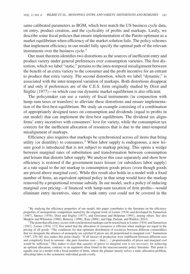
We now assess the welfare costs of monopolistic competition under C.E.S.-DS preferences when combined with endogenous labor and endogenous physical capi-tal investment (in turn). In other words, we assess the quantitative significance of the distortions analyzed in Sections IIIA and IIIB above under our baseline calibration, when these distortions operate in isolation.

Figure 2 plots our welfare-cost measure for the case of elastic labor (see Section IIIA under C.E.S.-DS). The upper panel plots the welfare cost as a function of the inverse consumption labor supply elasticity φ ( = − U LL L/ U L ) for the base-line calibration given above. The lower panel plots the welfare cost as a function of the steady-state markup μ − 1 = (θ − 1) −1 . (Our calibrated markup for C.E.S.-DS preferences is μ − 1 = 0.36 given θ = 3.8 ). In this panel, we hold the elasticity φ constant at its previously calibrated level (0 .25 in BGM). These two graphs illustrate

24 In a model with nominal rigidities, this further implies that the degree of regulation is a key determinant of the optimal inflation rate, as noted by Bilbiie, Fujiwara, and Ghironi (2014).

5 35

30

25

20

15

10

5

0

4

3

2

1

0 2 104 6 8 0.2 10.4 0.6 0.8

Wel

fare

gai

ns (p

erce

nt)

C.E.S.–DS, elastic labor

Wel

fare

gai

ns (p

erce

nt)

φ � − 1

Figure 2. Efficiency Gains Relative to Market Equilibrium: Elastic Labor


the complementarity between elastic labor and monopoly power in the goods market in generating distortions and welfare costs: the more elastic is labor (the lower the φ ) and the larger the markup, the higher the welfare cost—through the mechanism we previously emphasized. For our baseline calibration with φ = 0.25 and θ = 3.8 , the welfare cost associated to this distortion is around 5 percent. Even when the elasticity is very low, such as φ = 5, the cost is still 1 percent, vanishing only when labor supply becomes perfectly inelastic.

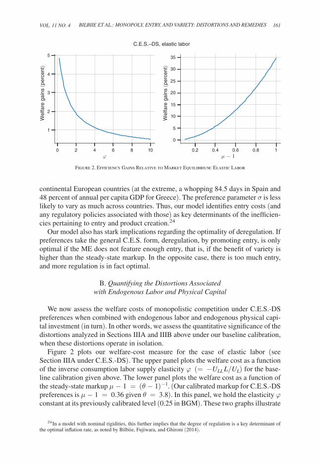
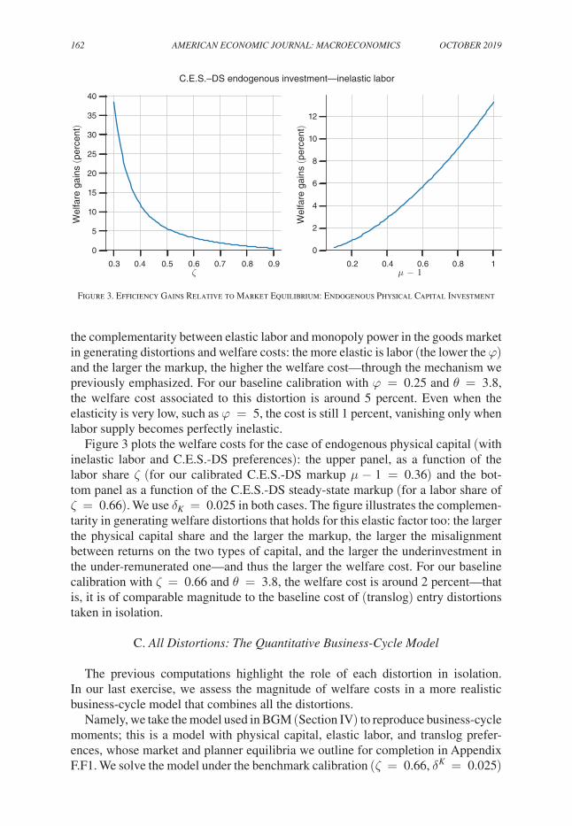
Figure 3 plots the welfare costs for the case of endogenous physical capital (with inelastic labor and C.E.S.-DS preferences): the upper panel, as a function of the labor share ζ (for our calibrated C.E.S.-DS markup μ − 1 = 0.36 ) and the bot-tom panel as a function of the C.E.S.-DS steady-state markup (for a labor share of ζ = 0.66). We use δ K = 0.025 in both cases. The figure illustrates the complemen-tarity in generating welfare distortions that holds for this elastic factor too: the larger the physical capital share and the larger the markup, the larger the misalignment between returns on the two types of capital, and the larger the underinvestment in the under-remunerated one—and thus the larger the welfare cost. For our baseline calibration with ζ = 0.66 and θ = 3.8 , the welfare cost is around 2 percent—that is, it is of comparable magnitude to the baseline cost of (translog) entry distortions taken in isolation.

C. All Distortions: The Quantitative Business-Cycle Model

The previous computations highlight the role of each distortion in isolation. In our last exercise, we assess the magnitude of welfare costs in a more realistic business-cycle model that combines all the distortions.

Namely, we take the model used in BGM (Section IV) to reproduce business-cycle moments; this is a model with physical capital, elastic labor, and translog prefer-ences, whose market and planner equilibria we outline for completion in Appendix F.F1. We solve the model under the benchmark calibration ( ζ = 0.66 , δ K = 0.025 )

0

0.3 0.4 0.5 0.6 0.7 0.8 0.9 0.2 0.4 0.6 0.8 1

5

10

15

20

25

30

40

12

10

8

6

4

2

0

Wel

fare

gai

ns (p

erce

nt)

Wel

fare

gai

ns (p

erce

nt)

C.E.S.–DS endogenous investment—inelastic labor

35

ζ � − 1

Figure 3. Efficiency Gains Relative to Market Equilibrium: Endogenous Physical Capital Investment


and plot the welfare costs as a function of the key translog parameter σ/ f E for two values of labor elasticity: the value from BGM, φ −1 = 4 ( solid blue line), and a lower bound value φ −1 = 0.2 ( red dashed line).

In this case, all distortions coexist and interact: static and dynamic entry dis-tortions are due to markups being higher (double) on average than the benefit of variety and varying over the cycle; the labor-markup distortion operates insofar as labor supply is elastic and there is monopoly power in the goods market; and there is physical capital underinvestment since this capital provides inefficiently low return compared to the (monopoly) return on new varieties. For the baseline calibration with φ = 0.25 (blue curve) and σ/ f E = 0.354 ( vertical dashed line, see discussion above), the welfare cost associated with all these joint distortions is very large: 25 percent! Even when the labor elasticity is very low ( φ −1 = 0.2 , orange dashed line), the welfare costs are still substantial: around 7 percent. As we have previously motivated, these costs decrease with lower average markups (higher σ/ f E ). But, as we have argued, lower values of σ/ f E closer to our 0.35 choice ( gray dashed line) are needed to fit the empirical business cycle properties for markups. Thus, the combined distortions associated with entry and variety in the presence of monopoly power (and elastic factors of production) are likely to be substantial.

V. Conclusions

This paper contributes to the literature on the efficiency properties of models with monopolistic competition that can be traced back to Robinson (1933) and Lerner (1934). We studied the efficiency properties of a DSGE macroeconomic model with monopolistic competition and firm entry subject to sunk costs, a time-to-build lag, and exogenous risk of firm destruction.

Our main theoretical result is a theorem stating that, unless preferences for vari-ety follow the knife-edge C.E.S. form studied by Dixit and Stiglitz (1977), the mar-ket equilibrium is inefficient because of two distortions: a static one, pertaining to the difference between the consumer surplus from a new variety, and the market incentive to create that variety; and a dynamic one, stemming from the inefficiency of markup variation over time. Properly designed taxes can eliminate these distor-tions by inducing markup synchronization across time and states, and aligning the consumer surplus and profit destruction effects of firm entry; one example we pro-vide consists of a combination of consumption and dividend taxes.

When factors of production are elastic, two new distortions arise under monop-olistic competition, even under C.E.S.-DS preferences: because investment in intangible capital associated with the blueprints for new goods is subject to monop-oly rents, whereas the other factors (labor and physical capital) are not, there is underinvestment in those latter two factors—and thus underproduction relative to a planner’s allocation. An important property of optimal taxes in the presence of entry is that—to restore optimality—they should be designed so as to preserve the entry incentives tied to ex post monopoly profits. Thus, a policy of eliminating markups, and inducing marginal-cost pricing, would affect firms’ entry incentives and have undesirable effects; whereas a policy of subsidizing labor and physical capital can restore optimality without affecting the entry margin.


We provide a quantification of the welfare costs associated with all these dis-tortions—separately, and then jointly—in a calibrated version of our model. This reveals that, on its own, the entry distortion accounts for a roughly 2 percent welfare loss. On their own, distortions associated with elastic labor and physical investment account for welfare losses around 5 percent and 2 percent (respectively). However, the welfare losses are greatly magnified when they jointly coexist. In that case, the welfare loss jumps up to 25 percent.

As we have previously discussed, the parametrization of preferences induces a specific functional form governing the benefit of new varieties. Although there is an extensive empirical literature quantifying the benefits of new goods with observ-able product characteristics (see Hausman 1997 for an early example), there is still very little understanding of the appropriate functional forms—and its associated parameter values—for this welfare impact at more aggregated levels when such product characteristics are not available.25 This stands in contrast to the measure-ment of product substitutability, where there is much more understanding of various functional forms and their associated parameter values at the macroeconomic level. This, in turn, has direct implications for the parametrization of markups and profits. Although we have highlighted in our previous work (see BGM) how the translog functional form does a good job of matching those business cycle properties for markups and profits (as well as entry), we do not know whether the normative prop-erties of this functional form provide a good empirical fit.26 Our findings thus point to the need for further empirical research on the appropriate modeling assumptions for the aggregate welfare impact of fluctuations in product variety.

Appendix A. Homothetic Consumption Preferences

Consider an arbitrary set of homothetic preferences over a continuum of goods Ω . Let p(ω) and c(ω) denote the prices and consumption level (quantity) of an indi-vidual good ω ∈ Ω . These preferences are uniquely represented by a price index function P ≡ h(p), p ≡ [ p(ω)] ω∈Ω , such that the optimal expenditure function is given by PC , where C is the consumption index (the utility level attained for a monotonic transformation of the utility function that is homogeneous of degree 1 ). Any function h(p) that is nonnegative, non-decreasing, homogeneous of degree 1 , and concave, uniquely represents a set of homothetic preferences. Using the conven-tional notation for quantities with a continuum of goods as flow values, the derived Marshallian demand for any variety ω is then given by

c (ω) dω = C ∂ P _ ∂ p (ω) .

25 In part, this is due to the relative novelty of macroeconomic models with endogenous product variety.26 This is indeed the reason why we have reported our quantification of those normative properties for alterna-

tive functional forms.


Appendix B. No Option Value of Waiting to Enter

Let the option value of waiting to enter for firm ω be Λ t (ω) ≥ 0 . In all periods t , Λ t (ω) = max[ v t (ω) − w t f E,t / Z t , β Λ t+1 (ω)], where the first term is the payoff of undertaking the investment and the second term is the discounted payoff of waiting. If firms are identical (there is no idiosyncratic uncertainty) and exit is exogenous (uncertainty related to firm death is also aggregate), this becomes: Λ t = max[ v t − w t f E,t / Z t , β Λ t+1 ] . Because of free entry, the first term is always zero, so the option value obeys: Λ t = β Λ t+1 . This is a contraction mapping because of discounting, and by forward iteration, under the assumption lim T→∞ β T Λ t+T = 0 (i.e., there is a zero value of waiting when reaching the terminal period), the only stable solution for the option value is Λ t = 0 .

Appendix C. Derivations for Market Equilibrium and Planner Problem

The market equilibrium is summarized by Table C1.27

We can reduce the system in Table C1 to a system of two equations in two vari-ables, N t and C t . To see this, write firm value as a function of the endogenous state N t and the exogenous state f E by combining free entry, pricing, variety, and markup equations:

(C1) v t = f E ρ ( N t )

_ μ ( N t ) .

Substituting this, together with the profits’ definition, in the Euler equation, we obtain (3) in text.

The first-order condition for the planner’s problem (5) is

U′ ( C t ) Z t ρ ( N t ) 1 _ 1 − δ f E

_ Z t

= β E t {U′ ( C t+1 ) Z t+1 ρ′ ( N t+1 )

× [L − 1 _ (1 − δ)

f E _ Z t+1 N t+2 +

f E _ Z t+1 N t+1 +

f E _ Z t+1 ρ ( N t+1 )

_______ ρ′ ( N t+1 ) ] } .

The term in square brackets in the right-hand side of this equation is

L − 1 _ (1 − δ)

f E _ Z t+1 N t+2 +

f E _ Z t+1 N t+1 +

f E _ Z t+1 ρ ( N t+1 )

_______ ρ′ ( N t+1 ) = L t+1

C + f E _ Z t+1 ρ ( N t+1 )

_______ ρ′ ( N t+1 ) .

27 The labor market equilibrium condition is redundant once the variety effect equation is included in the system in Table 2.


Hence, the first-order condition becomes

U′ ( C t ) ρ ( N t ) f E,t = β (1 − δ) E t {U′ ( C t+1 ) Z t+1 ρ′ ( N t+1 ) [ L t+1 C +

f E _ Z t+1 ρ ( N t+1 )

_______ ρ′ ( N t+1 ) ] } ,

leading to (6).

Appendix D. Proof of Theorem 1

Sufficiency (if) is directly verified by plugging conditions (i) and (ii) into (3) and (6).

Necessity (only if) requires that, whenever both (3) and (6) are satisfied, (i) and (ii) hold. We prove this by contradiction. We first look at the simpler perfect-foresight case (where we can drop the expectations operator) and then extend our proof to the stochastic case.

Suppose by reductio ad absurdum that there exists a 2-tuple {C t , N t+1 } that is both a ME and a PE, with μ( N t ) ≠ μ( N t+1 ) or ϵ(x) ≠ μ(x) − 1 or both. We examine each case separately.

(A) μ ( N t ) ≠ μ ( N t+1 ) and ϵ (x) = μ (x) − 1 :

Substituting ϵ( N t+1 ) in the planner’s Euler equation, μ( N t ) ≠ μ( N t+1 ) and ϵ(x) = μ(x) − 1 imply that

(D1) U′ ( C t+1 ) f E ρ ( N t+1 ) [ μ ( N t+1 ) − μ ( N t )

_____________ μ ( N t+1 ) ]

= U′ ( C t+1 ) C t+1 _ N t+1

(μ ( N t+1 ) − μ ( N t ) ) (

1 _ μ ( N t+1 ) − 1

) .

Table C1—Model Summary

Pricing ρ t = μ t w t _ Z t

Variety effect ρ t = ρ ( N t )

Markup μ t = μ ( N t )

Profits d t = (1 − 1 _ μ t ) C t _ N t

Free entry v t = w t f E

_ Z t

Number of firms N t = (1 − δ) ( N t−1 + N E,t−1 )

Euler equation v t = β (1 − δ) E t [ U ′ ( C t+1 )

_ U ′ ( C t )

( v t+1 + d t+1 ) ]

Aggregate accounting C t + N E,t v t = w t L + N t d t


After further simplification, using μ( N t ) ≠ μ( N t+1 ) and U′( C t+1 ) ≠ 0 , this yields

(D2) 1 − μ ( N t+1 ) = f E ρ ( N t+1 ) N t+1

____________ C t+1

≤ 0, since μ ( N t+1 ) ≥ 1.

But this is a contradiction, since all terms on the right-hand side are strictly positive.

For the stochastic case:

E t {U′ ( C t+1 ) μ ( N t+1 ) − μ ( N t )

_____________ μ ( N t+1 ) [ f E ρ ( N t+1 ) +

C t+1 _ N t+1 (μ ( N t+1 ) − 1) ] } = 0,

which is a contradiction since μ( N t ) ≠ μ( N t+1 ) , U′( C t+1 ) ≠ 0 , and the term in square brackets is strictly greater than zero ( μ( N t+1 ) ≥ 1 ).

(B) μ ( N t ) = μ ( N t+1 ) = μ and ϵ (x) ≠ μ (x) − 1 :

Using Theorem 1, μ( N t ) = μ( N t+1 ) = μ and ϵ(x) ≠ μ(x) − 1 imply that

(D3) U′ ( C t+1 ) C t+1 _ N t+1

[ϵ ( N t+1 ) − (μ − 1) ] = 0.

This would further imply that either U′( C t+1 ) = 0 or C t+1 = 0 or ϵ( N t+1 ) = μ − 1 ,which are all contradictions.

(C) μ ( N t ) ≠ μ ( N t+1 ) and ϵ (x) ≠ μ (x) − 1 :

In this case, a steady state is still defined by N t = N t+1 , so μ( N t ) = μ( N t+1 ) = μ(N ) in steady state. If the ME and PE equilibria are identical, then (eval-uating the Euler equations at the steady state) ϵ(N ) = μ(N ) − 1 , which con-tradicts the assumption ϵ(x) ≠ μ(x) − 1. This holds for the stochastic case too (note that the same argument can be used in part (B), including the stochastic case). ∎

Appendix E. Endogenous Labor Supply

From inspection of Table C1, the two modifications to the CE conditions implied by endogeneity of labor supply are that L in the aggregate accounting identity now features a time index t, and the marginal utility of consumption, now denoted by U C ( C t , L t ), depends on hours worked. The new variable L t is then determined in stan-dard fashion by adding to the equilibrium conditions the intra-temporal first-order condition of the household governing the choice of labor effort:

− U L ( C t , L t ) = w t U C ( C t , L t ) .


Combining this with the wage schedule w t = Z t ρ( N t )/μ( N t ) , which holds also with endogenous labor supply, yields the condition

− U L ( C t , L t ) / U C ( C t , L t ) = Z t ρ ( N t ) /μ ( N t ) .

This, in turn, can be solved to obtain hours worked as a function of consumption, the number of firms, and productivity.

The PE when labor supply is endogenous is found by solving

max { L s , N s+1 } s=t

∞

E t ∑

s=t

∞ β s−t U [ Z s ρ ( N s ) ( L s − 1 _

(1 − δ) f E,s _ Z s

N s+1 + f E,s _ Z s

N s ) , L s ] .

The Euler equation for the planner’s optimal choice of N t+1 and the law of motion for the number of firms are identical to the case of fixed labor supply, up to the addition of a time index for labor and to recognizing the dependence of the marginal utility of consumption upon the level of effort. The additional intra-temporal condi-tion for the planning optimum is

− U L ( C t , L t ) / U C ( C t , L t ) = Z t ρ ( N t ) .

E1. Proof of Proposition 1

The profit function becomes: d t = (1 + τ t ) ρ t y t − w t l t − T t F or ( under optimal

pricing ρ t = μ( N t ) _____ 1 + τ t

w t _ Z t

), d t = (1 + τ t ) ρ t y t − (1 + τ t ) ______ μ( N t )

ρ t y t − T t F . Balanced budget

implies that total taxes are τ t ρ t N t y t , so the fraction of taxes paid by a firm is T t

F = γ t τ t ρ t y t . It follows that profits are finally given by

d t = [

1 + (1 − γ t ) τ t − 1 + τ t _ μ ( N t )

]

ρ t y t = [

1 + (1 − γ t ) τ t − 1 + τ t _ μ ( N t )

]

C t _ N t

.

To eliminate the wedge between the marginal rate of substitution and the marginal rate of transformation between consumption and leisure, we know that the optimal value of τ t is such that 1 + τ t = μ( N t ), implying d t = (1 − γ t ) (μ( N t ) − 1) ( C t / N t ). The value of a firm is given by v t = w t ( f E,t / Z t ) = ρ( N t ) f E,t . Substituting these expres-sions in the CE Euler equation for shares yields

U C ( C t , L t ) ρ ( N t ) f E,t

= β (1 − δ) E t { U C ( C t+1 , L t+1 )

× [ f E,t+1 ρ ( N t+1 ) + (1 − γ t+1 ) (μ ( N t+1 ) − 1) C t+1 _ N t+1

] } .


Comparing this with the planner’s Euler equation (6) written for the case of endog-enous labor (and hence replacing U′(C) with U C (C, L) ), we obtain the optimal frac-tion of taxes paid by the firm, γ t

∗ , as in the proposition. ∎

Appendix F. Endogenous Investment in Physical Capital

The market equilibrium is summarized by Table F1, where we have in addition to Table C1 the aggregate variables K, I , the price r K , and for convenience Y C,t and L C,t . (Note that the aggregate manufacturing production function can be replaced by the definition of manufacturing output, which is obtained by using other equilibrium conditions Y C,t = C t + I t . )

To solve the planner equilibrium, note that we can combine the following constraints:

N t+1 = (1 − δ) N t + (1 − δ) (L − L C,t ) Z t

___________ f E,t

,

K t+1 = (1 − δ K ) K t + I t ,

C t + I t = Z t ρ ( N t ) ( L C,t ) ζ K t 1−ζ ,

to get an expression for the control (consumption) as a function of the states:

C t = Z t ρ ( N t ) (L − 1 _ 1 − δ

f E _ Z t+1 N t+1 +

f E _ Z t N t )

ζ K t

1−ζ − K t+1 + (1 − δ K ) K t .

Table F1—Model with Physical Capital, Summary

Pricing ρ t = θ _ θ − 1 λ t

Variety effect ρ t = N t 1 _ θ−1

Profits d t = (1 − 1 _ μ t ) Y C,t _ N t

Free entry v t = f E w t _ Z t

Number of firms N t = (1 − δ) ( N t−1 + N E,t−1 )

Euler equation (shares) v t = β (1 − δ) E t [ U C ( C t+1 )

_ U C ( C t )

( v t+1 + d t+1 ) ]

Aggregate accounting C t + I t + N E,t v t = w t L + N t d t + r t K K t .

Labor market clearing L t = L C,t + N E,t f E

_ Z t

Euler equation (capital) 1 = β E t [

U C ( C t+1 ) _

U C ( C t ) ( r t+1

K + 1 − δ K ) ]

Rental rate r t K = (1 − ζ) θ − 1 _ θ

Y C,t _ K t

Capital accumulation K t+1 = (1 − δ K ) K t + I t

Wage w t = ζ θ − 1 _ θ Y C,t _ L C,t

Production function Y C,t Y C,t = ρ t Z t ( L C,t ) ζ K t 1−ζ


The Euler equation corresponding to N t+1 is (with C.E.S.-DS)

Z t ρ ( N t ) K t 1−ζ ζ ( L C,t ) ζ−1 1 _

1 − δ f E _ Z t

= β E t { U C ( C t+1 )

_ U C ( C t )

1 _ θ − 1 Z t+1 N t+1

1 ____ θ−1 −1

K t+1 1−ζ ( L C,t+1 ) ζ−1

× [ L C,t+1 + (θ − 1) ζ N t+1 f E _ Z t+1 ] } .

We can rewrite this using the manufacturing production function as

ζ Y C,t _ L C,t

1 _ 1 − δ f E

_ Z t = β E t {

U C ( C t+1 ) _

U C ( C t ) [ζ

Y C,t+1 _ L C,t+1

f E _ Z t+1 + 1 _ θ − 1

Y C,t+1 _ N t+1

] } ,

which is the same as the decentralized shares Euler equation in Table 3, in which one substitutes the expression for profits, the free entry condition and the expression for real wage.

The Euler equation for K t+1 is

1 = β E t { U C ( C t+1 )

_ U C ( C t )

[ (1 − ζ) Z t+1 N t+1 1 _ θ−1

( L C,t+1 ) ζ K t+1

−ζ + 1 − δ K ] }

= β E t { U C ( C t+1 )

_ U C ( C t )

[ (1 − ζ) Y C,t+1 _ K t+1

+ 1 − δ K ] } .

F1. All Distortions: General Preferences, Endogenous Labor, and Physical Capital Investment

The most general model for which we compute and report welfare costs in Figure 4 consists of putting together the three special cases analyzed previously: general homothetic preferences, endogenous labor, and endogenous physical capital investment. This is essentially the model in Section IV of BGM (2012) extended to general homothetic preferences. Since there is nothing of substance that is novel, we just outline the equilibrium conditions needed to solve the model for completion, for both the ME and the PE—where everything has been defined above, in particular the functions ϵ( · ), ρ( · ) , and μ( · ) in Table 1.


The following equations hold regardless of whether we are under the market or planner equilibrium:

(F1) N t+1 = (1 − δ) N t + (1 − δ) ( L t − L C,t ) Z t

___________ f E,t

,

K t+1 = (1 − δ K ) K t + I t ,

Y C,t = C t + I t ,

Y C,t = Z t ρ ( N t ) ( L C,t ) ζ K t 1−ζ .

In the market equilibrium (ME), it can furthermore be shown very easily that the following three conditions need to hold (these come from the Euler equation for

φ = 0.25

φ = 5

0σ/fE

Translog, endogenous investment—elastic labor

Wel

fare

gai

ns (p

erce

nt)

0

5

10

15

20

25

30

30

40

2 4 6 8 10

Figure 4. Efficiency Gains Relative to Market Equilibrium: All Distortions


new goods and physical capital respectively, and labor supply—having replaced the other static equilibrium conditions):

(F2) ζ Y C,t _ L C,t

f E

_ Z t = β (1 − δ) E t {

U C ( C t+1 )

_ U C ( C t )

[ζ Y C,t+1 _ L C,t+1

f E _ Z t+1 μ ( N t )

_ μ ( N t+1 )

+ μ ( N t ) (

1 − 1 _ μ ( N t+1 ) )

Y C,t+1 _ N t+1

] }

,

1 = β E t { U C ( C t+1 )

_ U C ( C t )

[ 1 _ μ ( N t+1 ) (1 − ζ)

Y C,t+1 _ K t+1 + 1 − δ K ] } ,

− U L ( L t ) = 1 _ μ ( N t ) ζ

Y C,t _ L C,t U C ( C t ) .

While for the planner equilibrium (PE), the three additional equilibrium condi-tions are instead

(F3) ζ Y C,t _ L C,t

f E

_ Z t = β (1 − δ) E t {

U C ( C t+1 ) _

U C ( C t ) [ζ

Y C,t+1 _ L C,t+1

f E _ Z t+1 + ϵ ( N t+1 )

Y C,t+1 _ N t+1 ] } ,

1 = β E t { U C ( C t+1 )

_ U C ( C t )

[ (1 − ζ) Y C,t+1 _ K t+1

+ 1 − δ K ] } ,

− U L ( L t ) = ζ Y C,t _ L C,t

U C ( C t ) .

An equilibrium consists of processes for the endogenous variables { N t , L t , L C,t , K t , C t , I t , Y C,t } that solve the four equations in (F1) and, respectively, the three equations in (F2) for the ME, or the three equations in (F3) for the PE–given initial conditions N 0 and K 0 and exogenous processes for Z t and f E,t .

REFERENCES

Acemoglu, Daron, Ufuk Akcigit, Harun Alp, Nicholas Bloom, and William Kerr. 2018. “Innovation, Reallocation, and Growth.” American Economic Review 108 (11): 3450–91.

Baqaee, David, and Emmanuel Farhi. 2018. “Productivity and Misallocation in General Equilibrium.” Unpublished.

Benassy, Jean-Pascal. 1996. “Taste for Variety and Optimum Production Patterns in Monopolistic Competition.” Economics Letters 52 (1): 41–47.

Bergin, Paul R., and Giancarlo Corsetti. 2008. “The Extensive Margin and Monetary Policy.” Journal of Monetary Economics 55 (7): 1222–37.

Bergin, Paul R., and Giancarlo Corsetti. 2014. “International Competitiveness and Monetary Policy.” old.econ.ucdavis.edu/faculty/bergin/research/Bergin-Corsetti-061114-gc.pdf.

Bertoletti, Paolo, and Federico Etro. 2016. “Preferences, Entry, and Market Structure.” RAND Journal of Economics 47 (4): 792–821.

http://old.econ.ucdavis.edu/faculty/bergin/research/Bergin-Corsetti-061114-gc.pdf

http://pubs.aeaweb.org/action/showLinks?doi=10.1257%2Fmac.20170303&system=10.1257%2Faer.20130470&citationId=p_1

http://pubs.aeaweb.org/action/showLinks?doi=10.1257%2Fmac.20170303&crossref=10.1111%2F1756-2171.12155&citationId=p_6

http://pubs.aeaweb.org/action/showLinks?doi=10.1257%2Fmac.20170303&crossref=10.1016%2F0165-1765%2896%2900834-8&citationId=p_3

http://pubs.aeaweb.org/action/showLinks?doi=10.1257%2Fmac.20170303&crossref=10.1016%2Fj.jmoneco.2008.08.011&citationId=p_4


Bilbiie, Florin O., Ippei Fujiwara, and Fabio Ghironi. 2014. “Optimal Monetary Policy with Endoge-nous Entry and Product Variety.” Journal of Monetary Economics 64: 1–20.

Bilbiie, Florin O., Fabio Ghironi, and Marc J. Melitz. 2008. “Monetary Policy and Business Cycles with Endogenous Entry and Product Variety.” In NBER Macroeconomics Annual 2007, edited by Daron Acemoglu, Kenneth Rogoff, and Michael Woodford, 299–353. Chicago: University of Chi-cago Press.

Bilbiie, Florin O., Fabio Ghironi, and Marc J. Melitz. 2012. “Endogenous Entry, Product Variety, and Business Cycles.” Journal of Political Economy 120 (2): 304–45.

Bilbiie, Florin O., Fabio Ghironi, and Marc J. Melitz. 2019. “Monopoly Power and Endogenous Prod-uct Variety: Distortions and Remedies: Dataset.” American Economic Journal: Macroeconomics. https://doi.org/10.1257/mac.20170303.

Cacciatore, Matteo, Giuseppe Fiori, and Fabio Ghironi. 2016. “Market Deregulation and Optimal Monetary Policy in a Monetary Union.” Journal of International Economics 99: 120–37.

Cacciatore, Matteo, and Fabio Ghironi. 2012. “Trade, Unemployment, and Monetary Policy.” https://www.frbatlanta.org/-/media/documents/news/conferences/2012/intl-economics/Cacciatore.pdf.

Chugh, Sanjay, and Fabio Ghironi. 2018. “Optimal Fiscal Policy with Endogenous Product Variety.” Unpublished.

Colciago, Andrea. 2016. “Endogenous Market Structures and Optimal Taxation.” Economic Journal 126 (594): 1441–83.

Colciago, Andrea, and Federico Etro. 2010. “Endogenous Market Structures and Business Cycles.” Economic Journal 120 (549): 1201–33.

Cooke, Dudley. 2016. “Optimal Monetary Policy with Endogenous Export Participation.” Review of Economic Dynamics 21: 72–88.

Dixit, Avinash K., and Joseph E. Stiglitz. 1977. “Monopolistic Competition and Optimum Product Diversity.” American Economic Review 67 (3): 297–308.

Dhingra, Swati, and John Morrow. 2019. “Monopolistic Competition and Optimum Product Diversity under Firm Heterogeneity.” Journal of Political Economy 127 (1): 196–232.

Ebell, Monique, and Christian Haefke. 2009. “Product Market Deregulation and the U.S. Employment Miracle.” Review of Economic Dynamics 12 (3): 479–504.

Edmond, Chris, Virgiliu Midrigan, and Daniel Xu. 2018. “How Costly Are Markups?” Unpublished. Epifani, Paolo, and Gino Gancia. 2011. “Trade, Markup Heterogeneity and Misallocations.” Journal of

International Economics 83 (1): 1–13.Etro, Federico. 2016. “The Ramsey Model with Imperfect Competition and General Preferences.”

Economic Letters 145: 141–44.Etro, Federico, and Lorenza Rossi. 2015. “New-Keynesian Phillips Curve with Bertrand Competition

and Endogenous Entry.” Journal of Economic Dynamics and Control 51: 318–40.Faia, Ester. 2012. “Oligopolistic Competition and Optimal Monetary Policy.” Journal of Economic

Dynamics and Control 36 (11): 1760–74.Feenstra, Robert C. 2003. “A Homothetic Utility Function for Monopolistic Competition Models,

without Constant Price Elasticity.” Economics Letters 78 (1): 79–86.Grossman, Gene M., and Elhanan Helpman. 1991. Innovation and Growth in the Global Economy.

Cambridge: MIT Press.Hausman, Jerry A. 1997. “Valuation of New Goods under Perfect and Imperfect Competition.” In The

Economics of New Goods, edited by Timothy F. Bresnahan and Robert J. Gordon, 207–48. Chi-cago: University of Chicago Press.

Judd, Kenneth. 1985. “On the Performance of Patents.” Econometrica 53 (3): 567–85.Kim, Jinill. 2004. “What Determines Aggregate Returns to Scale?” Journal of Economic Dynamics

and Control 28 (8): 1577–94.Lerner, A.P. 1934. “The Concept Monopoly and the Measurement of Monopoly Power.” Review of

Economic Studies 1 (3): 157–75.Lewis, Vivien. 2013. “Optimal Monetary Policy and Firm Entry.” Macroeconomic Dynamics 17 (8):

1687–1710.Lewis, Vivien, and Roland Winkler. 2015. “Product Diversity, Demand Structure, and Optimal Taxa-

tion.” Economic Inquiry 53 (2): 979–1003.Lucas, Robert E., Jr. 1987. Models of Business Cycles. Oxford, UK: Basil Blackwell.Mankiw, N. Gregory, and Michael D. Whinston. 1986. “Free Entry and Social Inefficiency.” RAND

Journal of Economics 17 (1): 48–58.Opp, Marcus M., Christine A. Parlour, and Johan Walden. 2014. “Markup Cycles, Dynamic Misallo-

cation, and Amplification.” Journal of Economic Theory 154: 126–61.

https://doi.org/10.1257/mac.20170303

https://www.frbatlanta.org/-/media/documents/news/conferences/2012/intl-economics/Cacciatore.pdf

https://www.frbatlanta.org/-/media/documents/news/conferences/2012/intl-economics/Cacciatore.pdf

http://pubs.aeaweb.org/action/showLinks?doi=10.1257%2Fmac.20170303&crossref=10.2307%2F2967480&citationId=p_30


http://pubs.aeaweb.org/action/showLinks?doi=10.1257%2Fmac.20170303&crossref=10.1016%2Fj.red.2008.11.002&citationId=p_19

http://pubs.aeaweb.org/action/showLinks?doi=10.1257%2Fmac.20170303&crossref=10.1016%2Fj.jedc.2014.10.009&citationId=p_23


http://pubs.aeaweb.org/action/showLinks?doi=10.1257%2Fmac.20170303&crossref=10.1017%2FS1365100512000272&citationId=p_31

http://pubs.aeaweb.org/action/showLinks?doi=10.1257%2Fmac.20170303&crossref=10.1016%2Fj.red.2015.03.003&citationId=p_16

http://pubs.aeaweb.org/action/showLinks?doi=10.1257%2Fmac.20170303&crossref=10.1016%2Fj.jet.2014.09.001&citationId=p_35

http://pubs.aeaweb.org/action/showLinks?doi=10.1257%2Fmac.20170303&crossref=10.1111%2Fecin.12159&citationId=p_32

http://pubs.aeaweb.org/action/showLinks?doi=10.1257%2Fmac.20170303&crossref=10.1016%2Fj.jinteco.2010.10.005&citationId=p_21

http://pubs.aeaweb.org/action/showLinks?doi=10.1257%2Fmac.20170303&crossref=10.1016%2FS0165-1765%2802%2900181-7&citationId=p_25

http://pubs.aeaweb.org/action/showLinks?doi=10.1257%2Fmac.20170303&crossref=10.1016%2Fj.jmoneco.2014.02.006&citationId=p_7

http://pubs.aeaweb.org/action/showLinks?doi=10.1257%2Fmac.20170303&crossref=10.1111%2Fecoj.12293&citationId=p_14


http://pubs.aeaweb.org/action/showLinks?doi=10.1257%2Fmac.20170303&crossref=10.1016%2Fj.jinteco.2015.11.002&citationId=p_11


Robinson, Joan. 1933. The Economics of Imperfect Competition. Cambridge, UK: Cambridge Univer-sity Press.

Samuelson, Paul. 1947. Foundations of Economic Analysis. Cambridge: Harvard University Press.Spence, Michael. 1976. “Product Selection, Fixed Costs, and Monopolistic Competition.” Review of

Economic Studies 43 (2): 217–35.Zhelobodko, Evgeny, Sergey Kokovin, Mathieu Parenti, and Jacques-François Thisse. 2012. “Monopo-

listic Competition: Beyond the Constant Elasticity of Substitution.” Econometrica 80 (6): 2765–84.


http://pubs.aeaweb.org/action/showLinks?doi=10.1257%2Fmac.20170303&crossref=10.3982%2FECTA9986&citationId=p_39

monopoly power and endogenous product variety: distortions

Documents