lecture 8: market power: monopoly and...
TRANSCRIPT
Monopoly and Monopoly Power
Sources of Monopoly Power
The Social Costs of Monopoly Power
Monopsony and Monopsony Power
Limiting Market Power: The Antitrust Laws
LECTURE 8: Market Power: Monopoly
and Monopsony

2
Review of Perfect Competition
P = LMC = LRAC
Normal profits or zero economic profits in the long
run
Large number of buyers and sellers
Homogenous product
Perfect information
Firm is a price taker

Review of Perfect Competition
Q
P Market
D S
Q0
P0
Q
P Individual Firm
P0 D = MR = P
q0
LRAC LMC

4
Monopoly 독점
Monopoly
1. One seller - many buyers
2. One product (no good substitutes)
3. Barriers to entry
4. Price Maker
5
Monopoly
The monopolist is the supply-side of the market and
has complete control over the amount offered for
sale.
Monopolist controls price but must consider consumer
demand
Profits will be maximized at the level of output
where marginal revenue equals marginal cost.

6
Average & Marginal Revenue
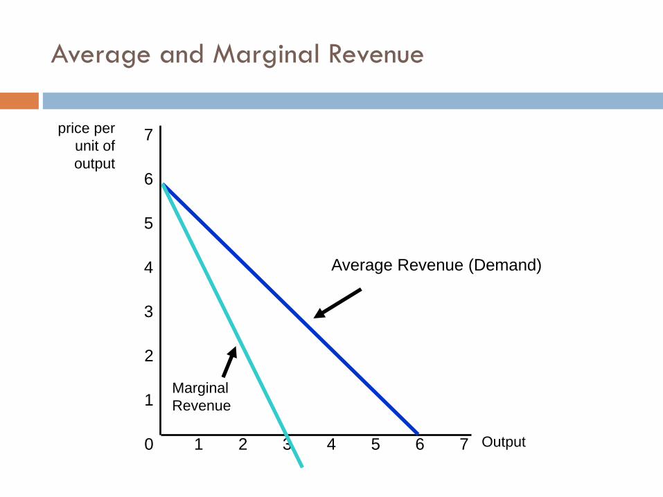
The monopolist’s average revenue, price received
per unit sold, is the market demand curve.
Monopolist also needs to find marginal revenue,
change in revenue resulting from a unit change in
output.
7
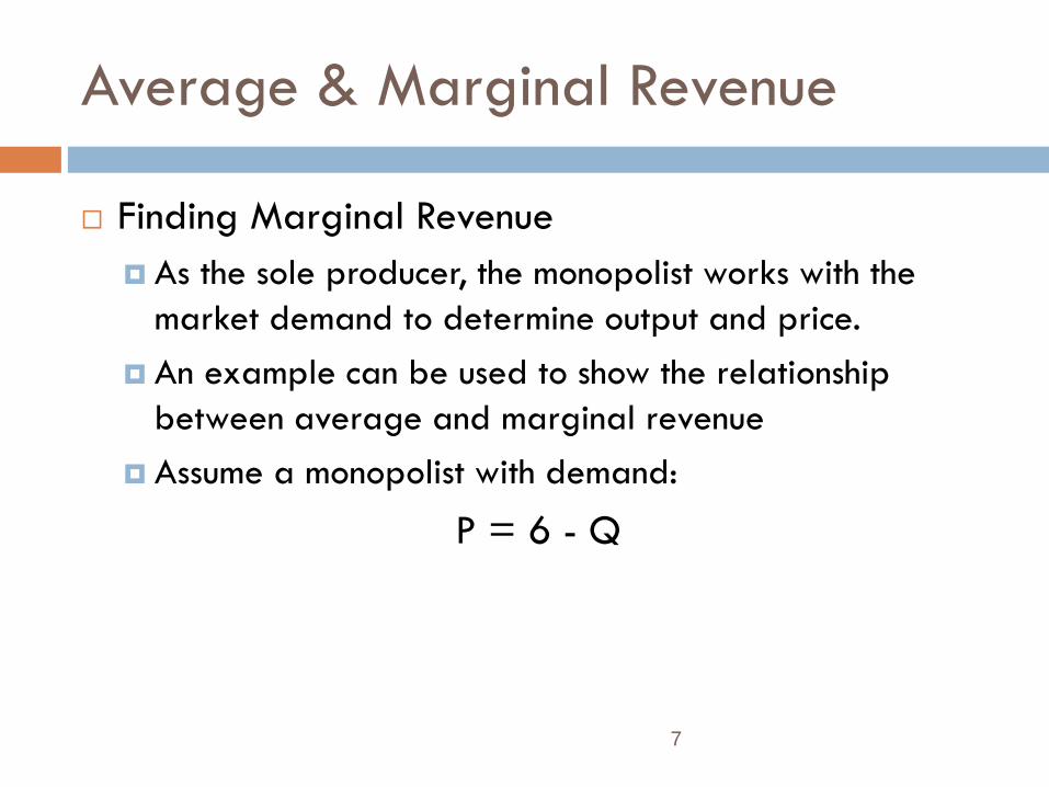
Average & Marginal Revenue
Finding Marginal Revenue
As the sole producer, the monopolist works with the
market demand to determine output and price.
An example can be used to show the relationship
between average and marginal revenue
Assume a monopolist with demand:
P = 6 - Q
Average and Marginal Revenue
Output 1 2 3 4 5 6 7 0
1
2
3
price per
unit of
output
4
5
6
7
Average Revenue (Demand)
Marginal
Revenue
9
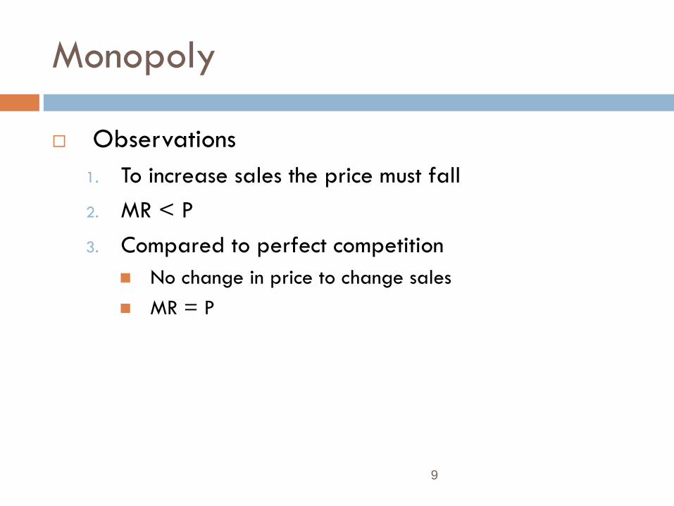
Monopoly
Observations
1. To increase sales the price must fall
2. MR < P
3. Compared to perfect competition
No change in price to change sales
MR = P
10
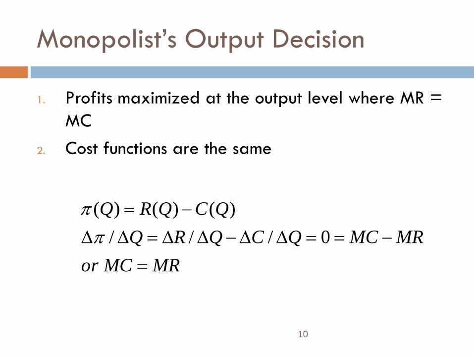
Monopolist’s Output Decision
1. Profits maximized at the output level where MR =
MC
2. Cost functions are the same
MRMCor
MRMCQCQRQ
QCQRQ
0///
)()()(

11
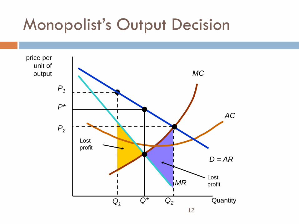
Monopolist’s Output Decision
At output levels below MR = MC the decrease in
revenue is greater than the decrease in cost (MR >
MC).
At output levels above MR = MC the increase in cost
is greater than the decrease in revenue (MR < MC)
12
Lost
profit
P1
Q1
Lost
profit
MC
AC
Quantity
price per
unit of
output
D = AR
MR
P*
Q*
Monopolist’s Output Decision
P2
Q2
13
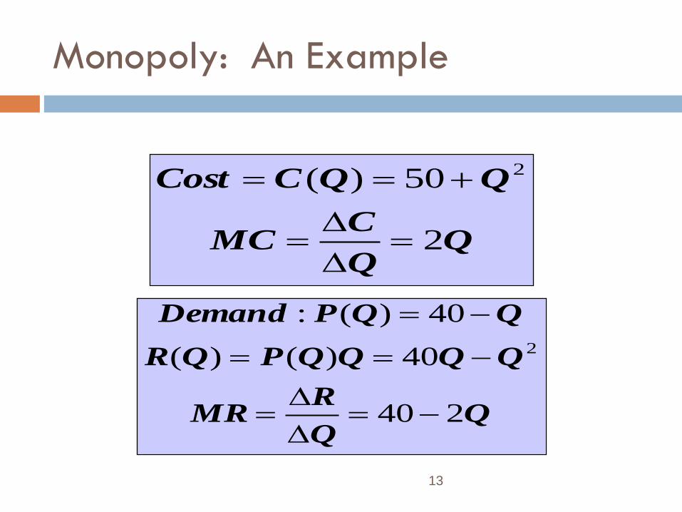
Monopoly: An Example
CMC
QQCCost
2
50)( 2
RMR
QQQQPQR
QQPDemand
240
40)()(
40)(:
2
14
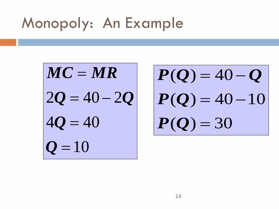
Monopoly: An Example
10
404
2402
Q
Q
MRMC
30)(
1040)(
40)(
QP
QP
QQP

15
Monopoly: An Example
By setting marginal revenue equal to marginal cost,
we verified that profit is maximized at P = 30 and
Q = 10.
This can be seen graphically by plotting cost,
revenue and profit
Profit is initially negative when produce little or no
output
Profit increase and q increase, maximized at Q*=10

16
Quantity 0 5 15 20
100
150
200
300
400
50
R
10
Profits
r
r'
c
c’
Example of Profit Maximization
C
When profits are
maximized, slope of
rr’ and cc’ are equal:
MR=MC
17
Profit
AR
MR
MC
AC
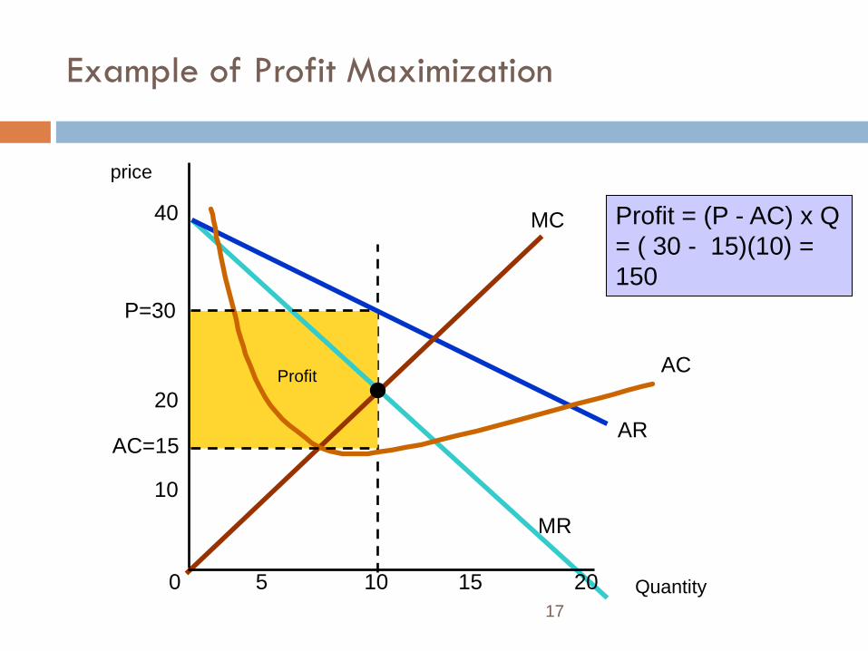
Example of Profit Maximization
Quantity 0 5 10 15 20
P=30
price
10
20
40
AC=15
Profit = (P - AC) x Q
= ( 30 - 15)(10) =
150
18
Monopoly
A Rule of Thumb for Pricing
We want to translate the condition that marginal
revenue should equal marginal cost into a rule of thumb
that can be more easily applied in practice.
Looking at Marginal Revenue we can see that it has two
components
19
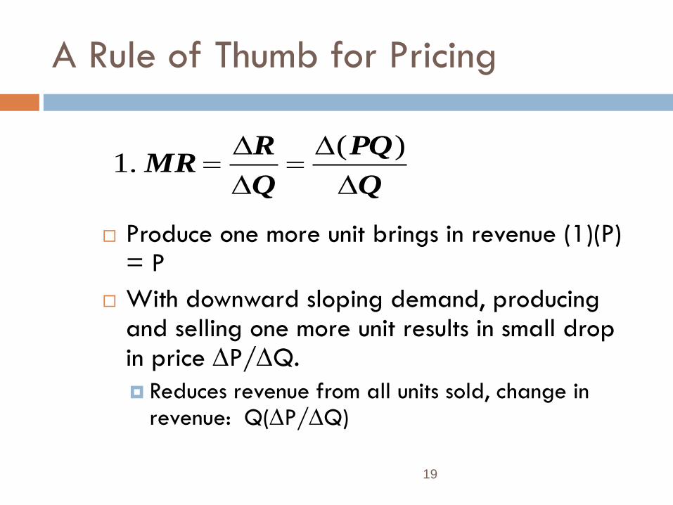
A Rule of Thumb for Pricing
Produce one more unit brings in revenue (1)(P) = P
With downward sloping demand, producing and selling one more unit results in small drop in price P/Q.
Reduces revenue from all units sold, change in revenue: Q(P/Q)
Q
PQ
Q
RMR
)(.1

20
A Rule of Thumb for Pricing
PQ
QPE
Q
P
P
QPP
Q
PQPMR
Thus
d.3
.2
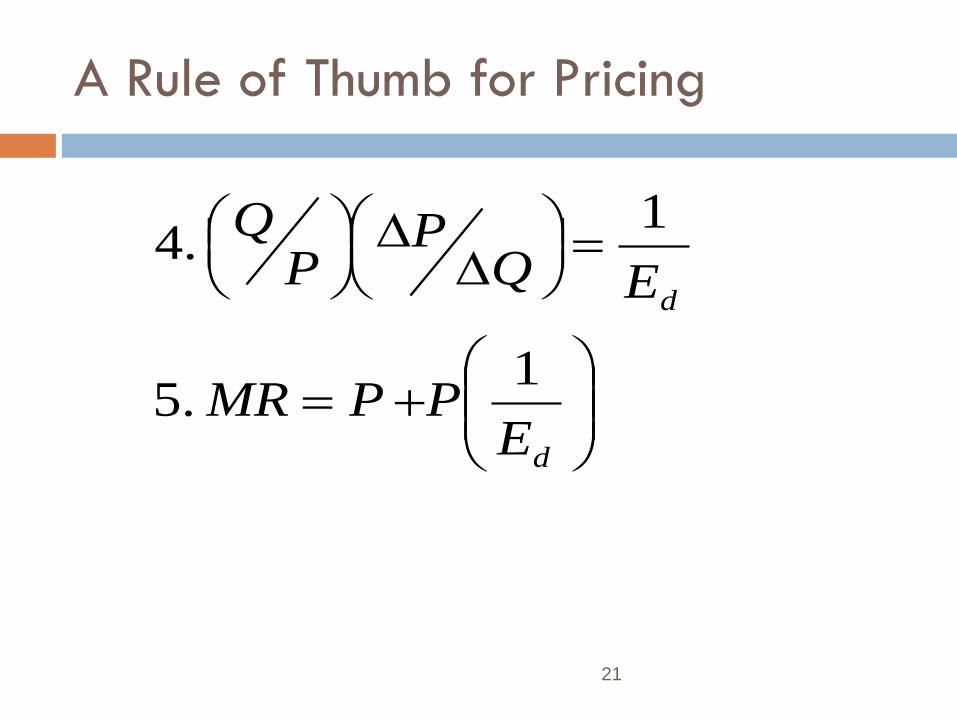
21
A Rule of Thumb for Pricing
d
d
EPPMR
EQP
PQ
1.5
1.4
22
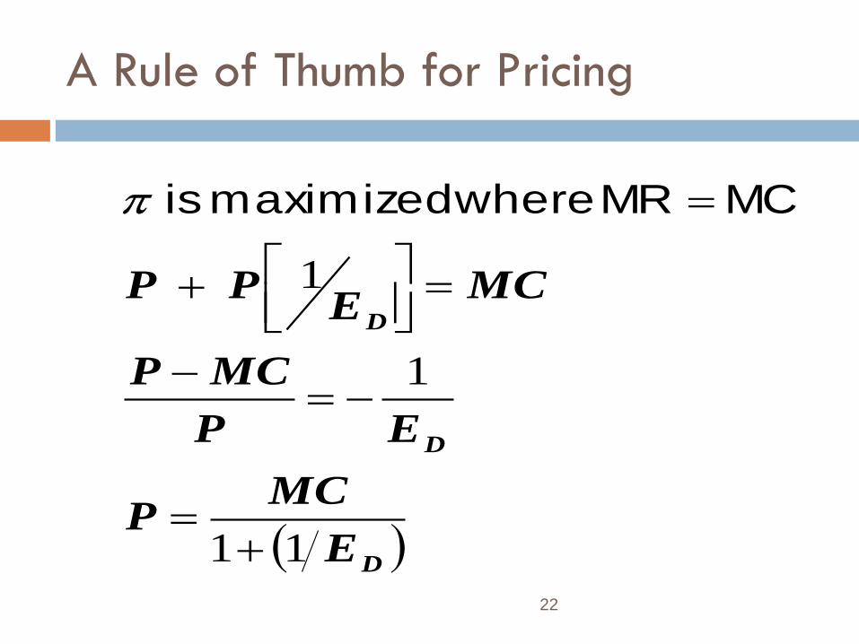
A Rule of Thumb for Pricing
D
D
D
E
MCP
EP
MCP
MCE
PP
11
1
1
MC MR wheremaximized is

23
A Rule of Thumb for Pricing
(P – MC)/P is the markup over MC as a percentage
of price
The markup should equal the inverse of the
elasticity of demand.
Price is expressed directly as the markup over
marginal cost
24
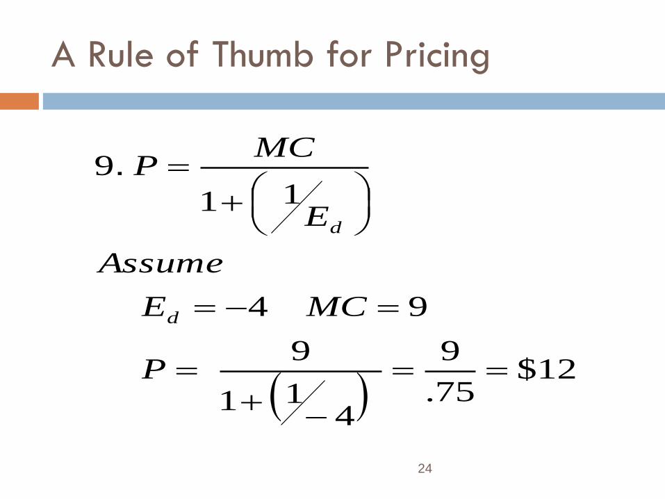
A Rule of Thumb for Pricing
12$
75.
9
411
9
94
11
9
.
P
MCE
Assume
E
MCP
d
d
25
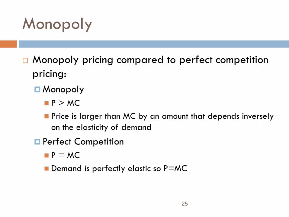
Monopoly
Monopoly pricing compared to perfect competition
pricing:
Monopoly
P > MC
Price is larger than MC by an amount that depends inversely
on the elasticity of demand
Perfect Competition
P = MC
Demand is perfectly elastic so P=MC

26
Monopoly
If demand is very elastic, there is little benefit to being a monopolist
The larger the elasticity, the closer to a perfectly competitive market
Notice a monopolist will never produce a quantity in the inelastic portion of demand curve
In inelastic portion, can increase revenue by decreasing quantity and increasing price
27
Shifts in Demand
In perfect competition, the market supply curve is
determined by marginal cost.
For a monopoly, output is determined by marginal
cost and the shape of the demand curve.
There is no supply curve for monopolistic market
28
Shifts in Demand
Shifts in demand do not trace out price and
quantity changes corresponding to a supply curve
Shifts in demand lead to
Changes in price with no change in output
Changes in output with no change in price
Changes in both price and quantity
29
D2
MR2
D1
MR1
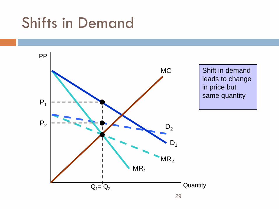
Shifts in Demand
Quantity
MC
PP
P2
P1
Q1= Q2
Shift in demand
leads to change
in price but
same quantity
30
D1
MR1
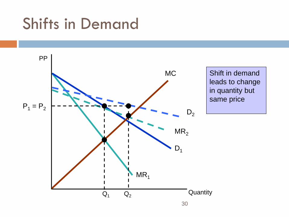
Shifts in Demand
MC
PP
MR2
D2
P1 = P2
Q1 Q2 Quantity
Shift in demand
leads to change
in quantity but
same price
31
Monopoly
Shifts in demand usually cause a change in both
price and quantity.
Example show how monopolistic market differs from
perfectly competitive market
Competitive market supplies specific quantity a
every price
This relationship does not exist for a monopolistic
market
32
The Effect of a Tax
In competitive market, a per-unit tax causes price to rise by less than tax: burden shared by producers and consumers
Under monopoly, price can sometimes rise by more than the amount of the tax.
To determine the impact of a tax:
t = specific tax
MC = MC + t
33
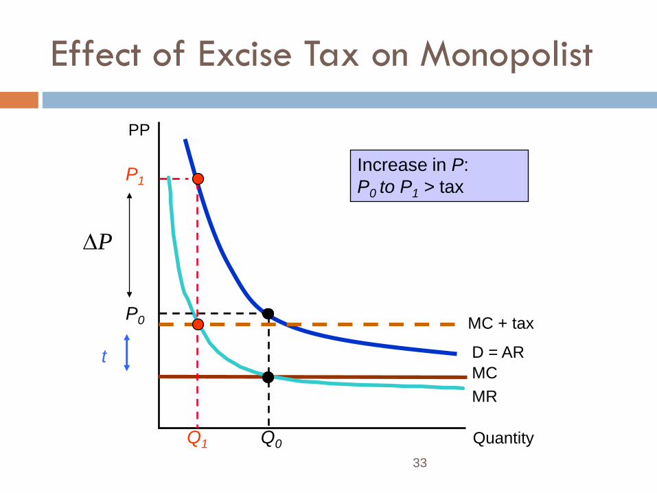
Effect of Excise Tax on Monopolist
Quantity
PP
MC
D = AR
MR
Q0
P0 MC + tax
t
P
Increase in P:
P0 to P1 > tax
Q1
P1

34
Effect of Excise Tax on Monopolist
The amount the price increases with implementation
of a tax depends on elasticity of demand
Price may or may not increase by more than the tax
In a competitive market, the price cannot increase
by more than tax
Profits for monopolist will fall with a tax
35
The Multi-plant Firm
For some firms, production takes place in more than one plant each with different costs
Firm must determine how to distribute production between both plants
1. Production should be split so that the MC in the plants is the same
2. Output is chosen where MR=MC. Profits is therefore maximized when MR=MC at each plant
36
The Multi-plant Firm
We can show this algebraically:
Q1 and C1 is output and cost of production for Plant 1
Q2 and C2 is output and cost of production for Plant 2
QT = Q1 + Q2 is total output
Profit is then:
= PQT – C1(Q1) – C2(Q2)
37
The Multi-plant Firm
Firm should increase output from each plant until the
additional profit from last unit produced at Plant 1
equals 0
1
1
1
1
11
0
0)(
MCMR
MCMR
Q
C
Q
PQ
Q
T

38
The Multi-plant Firm
We can show the same for Plant 2
Therefore we can see that the firm should choose to produce where
MR = MC1 = MC2
We can show this graphically
MR = MCT gives total output
This point shows the MR for each firm
Where MR crosses MC1 and MC2 shows the output for each firm

39
Production with Two Plants
Quantity
PP
D = AR
MR
MC1 MC2
MCT
MR*
Q1 Q2 QT
P*

40
Monopoly Power
Pure monopoly is rare.
However, a market with several firms, each facing a downward sloping demand curve will produce so that price exceeds marginal cost.
Firms often product similar goods that have some differences thereby differentiating themselves from other firms
41
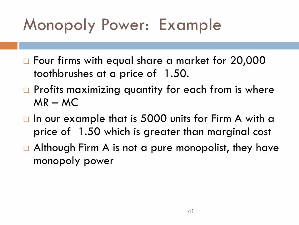
Monopoly Power: Example
Four firms with equal share a market for 20,000 toothbrushes at a price of 1.50.
Profits maximizing quantity for each from is where MR – MC
In our example that is 5000 units for Firm A with a price of 1.50 which is greater than marginal cost
Although Firm A is not a pure monopolist, they have monopoly power

At a market price
of 1.50, elasticity of
demand is -1.5. 2.00
P
1.50
1.00
Quantity 10,000 QA 20,000 30,000 3,000 5,000 7,000
P
2.00
1.50
1.00
1.40
1.60
DA
MRA
Market
Demand
Firm A has some monopoly power
and charges a price which
exceeds MC where MR=MC.
MCA
The Demand for Toothbrushes
43
Measuring Monopoly Power
Our firm would have more monopoly power of course if it
could get rid of the other firms
But the firm’s monopoly power might still be substantial
How can we measure monopoly power to compare firms
What are the sources of monopoly power?
Why do some firms have more than others?
44
Measuring Monopoly Power
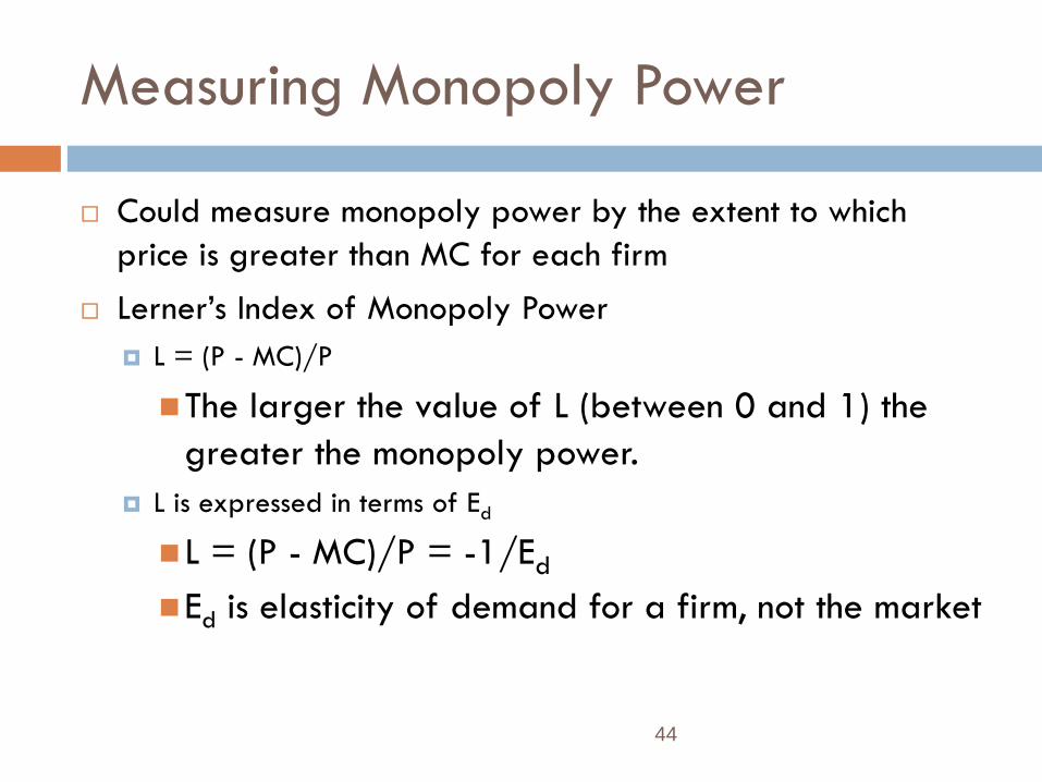
Could measure monopoly power by the extent to which
price is greater than MC for each firm
Lerner’s Index of Monopoly Power
L = (P - MC)/P
The larger the value of L (between 0 and 1) the
greater the monopoly power.
L is expressed in terms of Ed
L = (P - MC)/P = -1/Ed
Ed is elasticity of demand for a firm, not the market

45
Monopoly Power
Monopoly power, however, does not guarantee
profits.
Profit depends on average cost relative to price.
One firm may have more monopoly power, but
lower profits due to high average costs

46
Rule of Thumb for Pricing
Pricing for any firm with monopoly power
If Ed is large, markup is small
If Ed is small, markup is large
dE
MCP
11
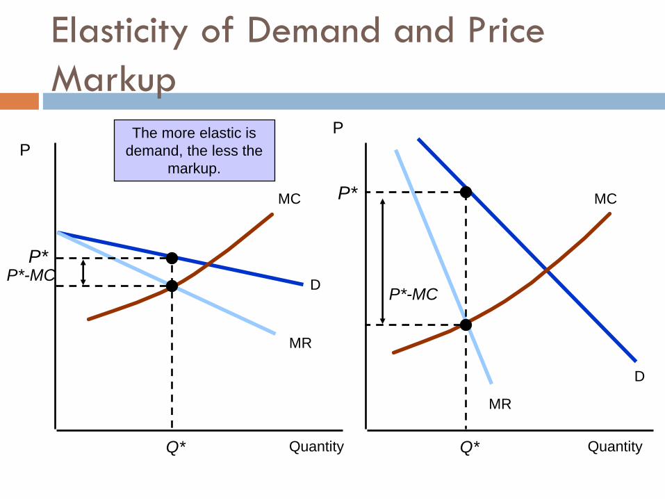
Elasticity of Demand and Price
Markup
P*
MR
D
P
Quantity
MC
Q*
P*-MC
The more elastic is
demand, the less the
markup.
D
MR
P
Quantity
MC
Q*
P* P*-MC

48
Markup Pricing: Supermarkets &
Convenience Stores
Supermarkets
MC. above 11%-10 about set Prices
stores individual for 3.
product Similar 2.
firms Several 1.
.5
)(11.19.01.11
.4
10
MCMCMC
P
Ed
49
Markup Pricing: Supermarkets &
Convenience Stores
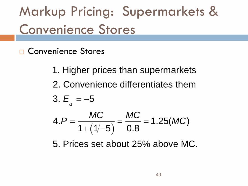
Convenience Stores
1. Higher prices than supermarkets
2. Convenience differentiates them
3. 5
4. 1.25( )1 1 5 0.8
5. Prices set about 25% above MC.
dE
MC MCP MC
50
Markup Pricing: Supermarkets &
Convenience Stores
Convenience stores have more monopoly power.
Convenience stores do have higher profits than
supermarkets however.
Volume is far smaller and average fixed costs are
larger
51
Sources of Monopoly Power
Why do some firm’s have considerable monopoly
power, and others have little or none?
Monopoly power is determined by ability to set
price higher than marginal cost
A firm’s monopoly power, therefore, is determined
by the firm’s elasticity of demand.
52
Sources of Monopoly Power
The less elastic the demand curve, the more
monopoly power a firm has.
The firm’s elasticity of demand is determined by:
1) Elasticity of market demand
2) Number of firms in market
3) The interaction among firms
53
Elasticity of Market Demand
With one firm their demand curve is market
demand curve
Degree of monopoly power determined completely by
elasticity of market demand
With more firms, individual demand may differ
from market demand
Demand for a firm’s product is more elastic than the
market elasticity
54
Number of Firms
The monopoly power of a firm falls as the number of firms increases all else equal
More important are the number of firms with significant market share
Market is highly concentrated if only a few firms account for most of the sales
Firms would like to create barriers to entry to keep new firms out of market
Patent, copyrights, licenses, economies of scale
55
Interaction Among Firms
If firms are aggressive in gaining market share by, for example, undercutting the other firms, prices may reach close to competitive levels.
If firms collude (violation of antitrust rules), could generate substantial monopoly power
Markets are dynamic and therefore, so is the concept of monopoly power
56
The Social Costs of Monopoly
Power
Monopoly power results in higher prices and lower
quantities.
However, does monopoly power make consumers
and producers in the aggregate better or worse
off?
We can compare producer and consumer surplus
when in a competitive market and in a monopolistic
market
57
The Social Costs of Monopoly
Perfectly competitive firm will produce where MC = D PC
and QC
Monopoly produces where MR = MC, getting their price
from the demand curve PM and QM
There is a loss in consumer surplus when going from perfect
competition to monopoly
A deadweight loss is also created with monopoly

58
B A
Lost Consumer Surplus Because of the
higher price,
consumers lose
A+B and producer
gains A-C.
C
Deadweight Loss from Monopoly
Power
Quantity
AR=D
MR
MC
QC
PC
Pm
Qm
P
Deadweight
Loss

59
The Social Costs of Monopoly
Social cost of monopoly is likely to exceed the
deadweight loss
Rent Seeking
Firms may spend to gain monopoly power
Lobbying
Advertising
Building excess capacity
60
The Social Costs of Monopoly
The incentive to engage in monopoly practices is
determined by the profit to be gained.
The larger the transfer from consumers to the firm,
the larger the social cost of monopoly.

61
The Social Costs of Monopoly
Example
1996 Archer Daniels Midland (ADM) successfully
lobbied for regulations requiring ethanol be produced
from corn
Although ethanol is the same whether produced from
corn, potatoes, grain or anything else, ADM had a near
monopoly on corn based ethanol production.
62
The Social Costs of Monopoly
Government can regulate monopoly power through
price regulation
Recall that in competitive markets, price regulation
created a deadweight loss.
Price regulation can eliminate deadweight loss with a
monopoly
We can show the effect of the regulation can be shown
graphically

63
AR
MR
MC Pm
Qm
AC
P1
Q1
Marginal revenue curve
when price is regulated
to be no higher that P1.
If left alone, a monopolist
produces Qm and charges Pm. If price is lowered to P3 output
decreases and a shortage exists.
For output levels above Q1 ,
the original average and
marginal revenue curves apply.
If price is lowered to PC output
increases to its maximum QC and
there is no deadweight loss.
Price Regulation
P
Quantity
P2 = PC
Qc
P3
Q3 Q’3
Any price below P4 results
in the firm incurring a loss.
P4
64
The Social Costs of Monopoly
Power
Natural Monopoly
A firm that can produce the entire output of an industry
at a cost lower than what it would be if there were
several firms.
Usually arises when there are large economies of scale
We can show that splitting the market into two firms
results in higher AC for each firm than when only one
firm was producing
65
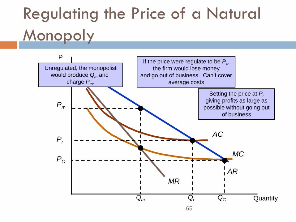
MC
AC
AR
MR
P
Quantity
Setting the price at Pr
giving profits as large as
possible without going out
of business
Qr
Pr
PC
QC
If the price were regulate to be Pc,
the firm would lose money
and go out of business. Can’t cover
average costs
Pm
Qm
Unregulated, the monopolist
would produce Qm and
charge Pm.
Regulating the Price of a Natural
Monopoly
66
The Social Costs of Monopoly
Power
Regulation in Practice
It is very difficult to estimate the firm's cost and demand
functions because they change with evolving market
conditions
An alternative pricing technique – rate-of-return
regulation allows the firms to set a maximum price
based on the expected rate or return that the firm will
earn.

67
Regulation in Practice
There are problems however with rate of return
regulation
1. Firm’s capital stock is difficult to value
2. “Fair” rate of return based on actual cost of capital,
that cost is based on regulatory behavior (and
investor’s perception of allowed rates in the future).

68
Regulation in Practice
Rate of return regulation leads to lags in regulatory
response to changes in cost and other market
conditions
Leads to long and expensive regulatory hearings.
The hearing process creates a regulatory lag that
may benefit producers (1950s & 60s) or consumers
(1970s & 80s).
69
Regulation in Practice
Government may also set price caps based on firms variable costs, past prices, and possibly inflation and productivity growth
A firm is typically allowed to raise its price each year without approval from regulatory agency by amount equal to inflation minus expected productivity growth

70
Monopsony
A monopsony is a market in which there is a single
buyer.
An oligopsony is a market with only a few buyers.
Monopsony power is the ability of the buyer to
affect the price of the good and pay less than the
price that would exist in a competitive market.
71
Monopsony
Typically choose to buy until the benefit from last unit equals that unit’s cost
Marginal value is the additional benefit derived from purchasing one more unit of a good
Demand curve – downward sloping
Marginal expenditure is the additional cost of buying one more unit of a good
Depends on buying power

72
Monopsony
Competitive Buyer
Price taker
P = Marginal expenditure = Average expenditure
D = Marginal value
Graphically can compare competitive buyer to
competitive seller
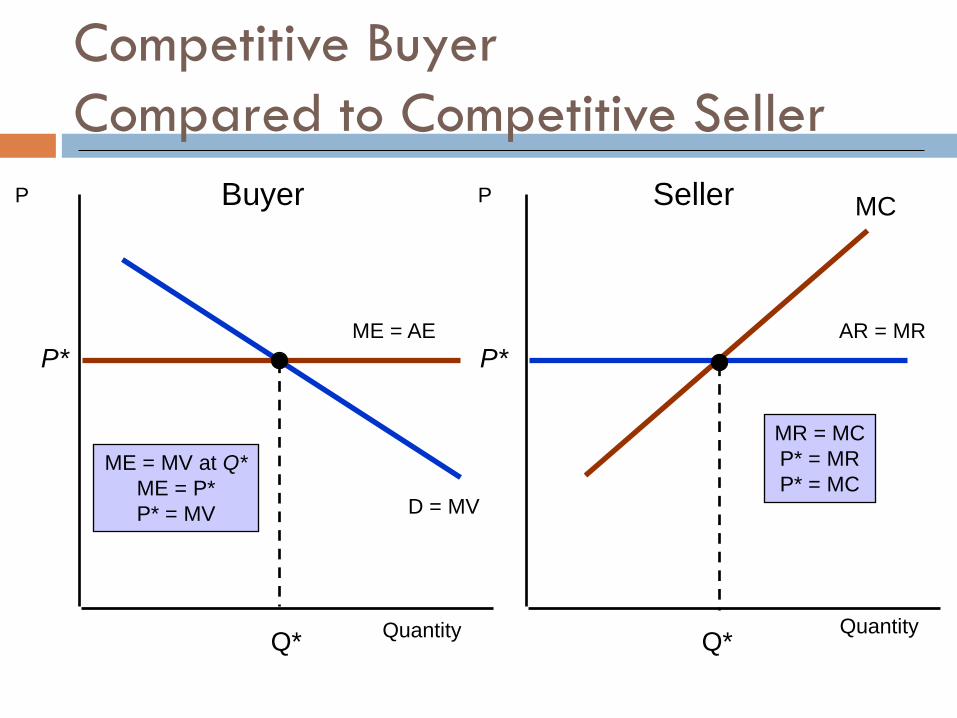
Competitive Buyer
Compared to Competitive Seller
Quantity Quantity
P P
D = MV
ME = AE
P*
Q*
ME = MV at Q*
ME = P*
P* = MV
AR = MR
P*
Q*
MC
MR = MC
P* = MR
P* = MC
Buyer Seller

74
Monopsonist Buyer
Buyer will buy until value from last unit equals expenditure
on that unit.
The market supply curve is not the marginal expenditure
curve
Market supply show how much must pay per unit as a function of
total units purchased
Supply curve is average expenditure curve
Upward sloping supply implies the marginal expenditure curve must
lie above it
Decision to buy extra unit raises price paid for all units

75
ME
S = AE
Monopsonist Buyer
Quantity
P
D = MV
Q*m
P*m
Monopsony
•ME above S
•Quantity where ME = MV: Qm
•Price from Supply curve: Pm
PC
QC
Competitive
•P = PC
•Q = Q+C
76
Monopoly and Monopsony
Monopsony is easier to understand if we compare to
monopoly
We can see this graphically
Monopolist
Can charge price above MC because faces downward sloping
demand (average revenue)
MR < AR
MR=MC gives quantity less than competitive market and price that is
higher

77
Monopoly and Monopsony
Quantity
Monopoly
Note: MR = MC;
AR > MR; P > MC
P
AR
MR
MC
QC
PC
P*
Q*
78
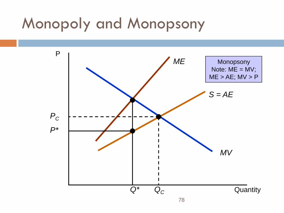
Monopoly and Monopsony
Quantity
P
MV
ME
S = AE
Q*
P*
PC
QC
Monopsony
Note: ME = MV;
ME > AE; MV > P

79
Monopoly and Monopsony
Monopoly
MR < P
P > MC
Qm < QC
Pm > PC
Monopsony
ME > P
P < MV
Qm < QC
Pm < PC
80
Monopsony Power
More common than pure monopsony are a few firm
competing among themselves as buyers so that each
firm has some monopsony power
Automobile industry
Monopsony power gives them the ability to pay a
price that is less than marginal value.
81
Monopsony Power
The degree of monopsony power depends on
three factors.
1. Number of buyers
The fewer the number of buyers, the less elastic the
supply and the greater the monopsony power.
2. Interaction Among Buyers
The less the buyers compete, the greater the monopsony
power.
82
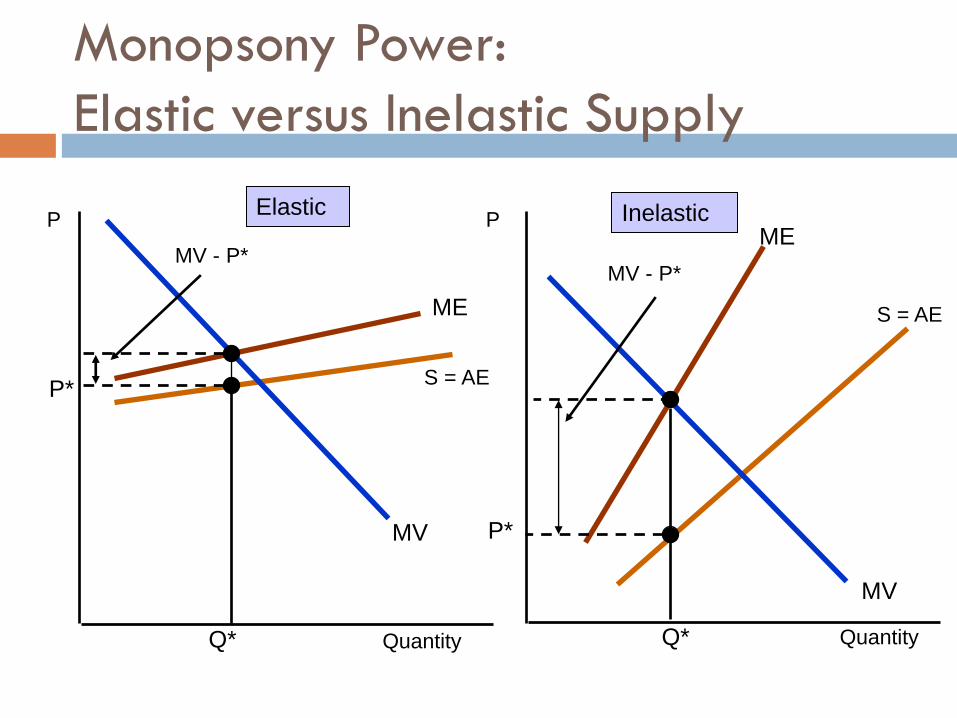
Monopsony Power
The degree of monopsony power depends
on three similar factors.
3. Elasticity of market supply
Extent to which price is marked down below MV
depends on elasticity of supply facing buyer
If supply is very elastic, markdown will be small
The more inelastic the supply the more monopsony
power
ME
S = AE
ME
S = AE
Monopsony Power:
Elastic versus Inelastic Supply
Quantity Quantity
P P
MV
MV
Q*
P*
MV - P*
P*
Q*
MV - P*
Elastic Inelastic

84
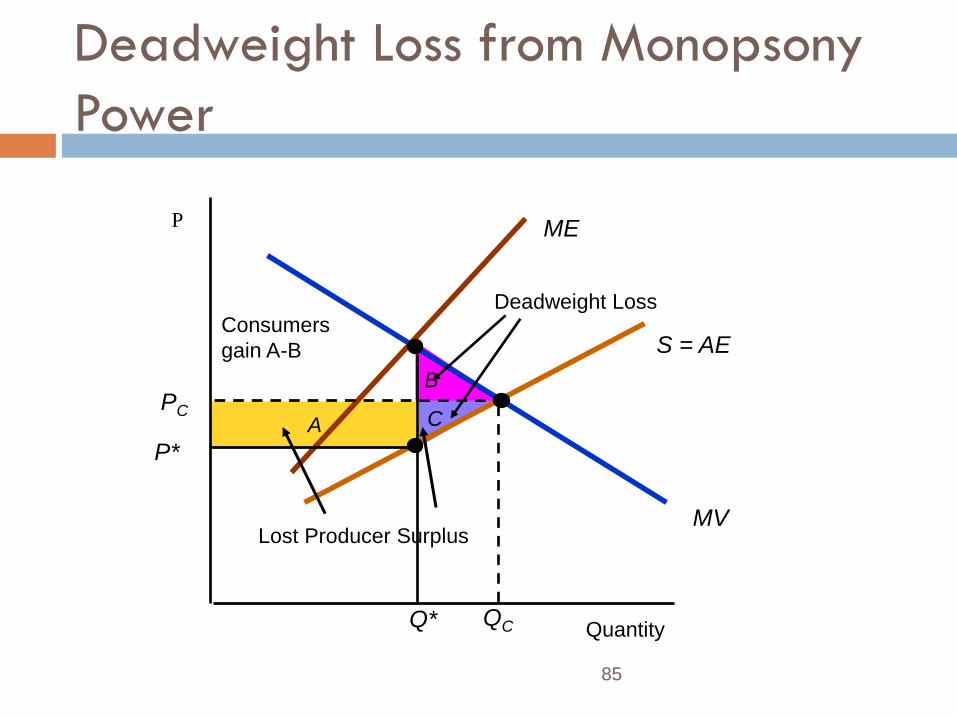
Social Costs of Monopsony Power
Since monopsony power gives lower prices and lower
quantities purchased, we would expect sellers to be worse
off and buyers better off
We can show effects of monopsony power using producer
and consumer surplus compared to competitive market
For sole monopsonist, quantity is where ME=MV and price is from
demand
For competitive market, quantity and price where S=D
85
C
B
Deadweight Loss from Monopsony
Power
A
Quantity
P
MV
ME
S = AE
PC
QC
Deadweight Loss Consumers
gain A-B
Q*
P*
Lost Producer Surplus
86
Monopsony Power
Bilateral Monopoly
Market where there is only one buyer and one seller
Bilateral monopoly is rare, however, markets with a small number of sellers with monopoly power selling to a market with few buyers with monopsony power is more common.
Even with bargaining, in general, monopsony and monopoly power will counteract each other
87
Limiting Market Power: The Antitrust
Laws
Market power harms some player in the market –
buyer or seller.
Market power reduces output leading to
deadweight loss
Excessive market power could raise problems of
equity and fairness
88
Limiting Market Power: The Antitrust
Laws
What can we do to limit market power and keep it from being used anti-competitively?
Tax away monopoly profits and redistribute to consumers
Difficult to measure and find all those who lost
Direct price regulation of natural monopolies
Keep firms from acquiring excessive market power
Antitrust laws

89
The Antitrust Laws
Rules and regulations designed to promote a
competitive economy by:
Prohibiting actions that restrain or are likely to restrain
competition
Restricting the forms of allowable market structures
Monopoly power arises in a number of ways, each
of which is covered by the antitrust laws
90
Limiting Market Power: The Antitrust
Laws
Sherman Act (1890) – Section 1
Prohibits contracts, combinations, or conspiracies in restraint of trade
Explicit agreement to restrict output or fix prices
Implicit collusion through parallel conduct
Form of implicit collusion in which one firm consistently follows actions of another
Example
In 1999, four of world’s largest drug and chemical companies found guilty of fixing prices of vitamins sold in US
91
Limiting Market Power:
The Antitrust Laws
Sherman Act (1890) – Section 2
Makes it illegal to monopolize or attempt to
monopolize a market and prohibits conspiracies that
result in monopolization.
Clayton Act (1914)
1. Makes it unlawful to require a buyer or lessor not to
buy from a competitor
92
Limiting Market Power:
The Antitrust Laws
Clayton Act (1914)
2. Prohibits predatory pricing
Practice of pricing to drive current competitors out of
business and to discourage new entrants in a market so
that a firm can enjoy higher future profits.
3. Prohibits mergers and acquisitions if they
“substantially lessen competition” or “tend to create a
monopoly”
93
Limiting Market Power:
The Antitrust Laws
Robinson-Patman Act (1936)
Amendment of the Clayton Act
Prohibits price discrimination if it causes buyers to suffer
economic damages and competition is reduced
94
Limiting Market Power:
The Antitrust Laws
Federal Trade Commission Act (1914, amended 1938, 1973, 1975)
1. Created the Federal Trade Commission (FTC)
2. Supplements the Sherman and Clayton acts by fostering competition through set of prohibitions against unfair and anticompetitive practices
Prohibitions against deceptive advertising, labeling, agreements with retailer to exclude competing brands
95
Enforcement of Antitrust Laws
Antitrust laws are enforced three ways:
1. Antitrust Division of the Department of Justice
A part of the executive branch – the administration
can influence enforcement
Fines levied on businesses; fines and imprisonment
levied on individuals
96
Enforcement of Antitrust Laws
2. Federal Trade Commission
Enforces through voluntary understanding or formal
commission order
3. Private Proceedings
Can sue for treble damages (three fold damages)
Individuals or companies can also ask for injunctions
to force wrongdoers to cease anticompetitive actions

97
Enforcement of Antitrust Laws
US antitrust laws are stricter and more far reaching
than the rest of the world
Some have claimed this has hindered US effectively
competing in international markets
With growth of European Union, methods of
antitrust enforcement have evolved
Similar to US laws with some procedural and
substantive differences
Europe only imposes civil penalties
98
Limiting Market Power:
The Antitrust Laws
Two Examples
American Airlines
Early 80’s president and CEO accused of attempting to
price fix
Microsoft
Monopoly power
Predatory actions
Collusion