More on single-view geometry

class 10

Multiple View GeometryComp 290-089Marc Pollefeys

Multiple View Geometry course schedule(subject to change)

Jan. 7, 9 Intro & motivation Projective 2D Geometry

Jan. 14, 16

(no class) Projective 2D Geometry

Jan. 21, 23

Projective 3D Geometry (no class)

Jan. 28, 30

Parameter Estimation Parameter Estimation

Feb. 4, 6 Algorithm Evaluation Camera Models

Feb. 11, 13

Camera Calibration Single View Geometry

Feb. 18, 20

Epipolar Geometry 3D reconstruction

Feb. 25, 27

Fund. Matrix Comp. Structure Comp.

Mar. 4, 6 Planes & Homographies Trifocal Tensor

Mar. 18, 20

Three View Reconstruction

Multiple View Geometry

Mar. 25, 27

MultipleView Reconstruction

Bundle adjustment

Apr. 1, 3 Auto-Calibration Papers

Apr. 8, 10

Dynamic SfM Papers

Apr. 15, 17

Cheirality Papers

Apr. 22, 24

Duality Project Demos

Single view geometry

Camera model

Camera calibration

Single view geom.

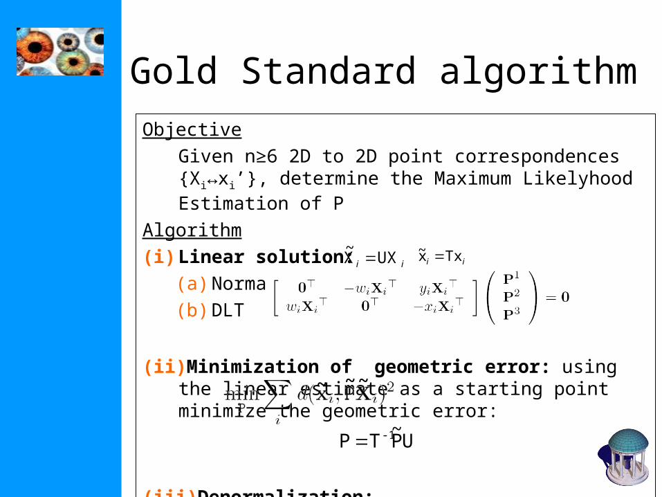
Gold Standard algorithmObjective

Given n≥6 2D to 2D point correspondences {Xi↔xi’}, determine the Maximum Likelyhood Estimation of P

Algorithm

(i) Linear solution:

(a) Normalization:

(b) DLT

(ii) Minimization of geometric error: using the linear estimate as a starting point minimize the geometric error:

(iii) Denormalization:

ii UXX~ ii Txx~

UP~

TP -1

~ ~~

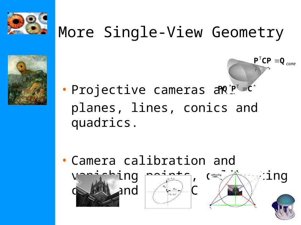
More Single-View Geometry

• Projective cameras and planes, lines, conics and quadrics.

• Camera calibration and vanishing points, calibrating conic and the IAC

** CPPQ T

coneQCPP T

Action of projective camera on planes

1ppp

10ppppPXx 4214321 Y

XYX

The most general transformation that can occur between a scene plane and an image plane under perspective imaging is a plane projective transformation

(affine camera-affine transformation)

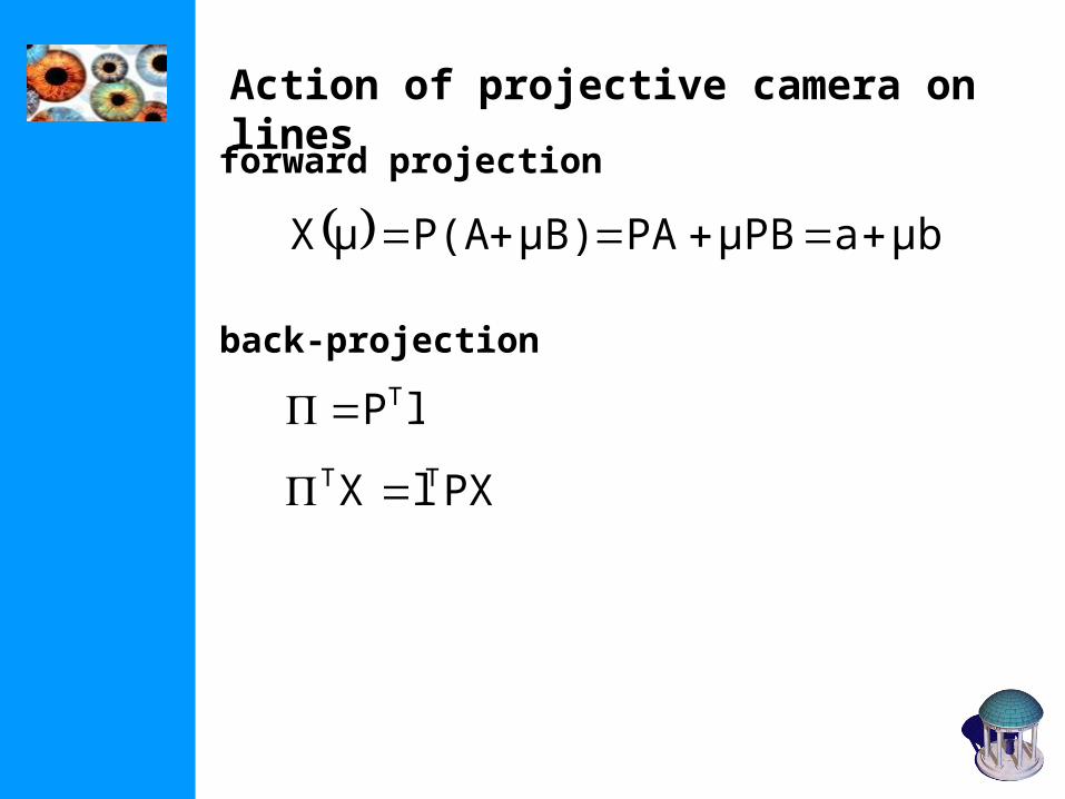
Action of projective camera on lines

forward projection

μbaμPBPAμB)P(AμX

back-projection

lPT

PXlX TT

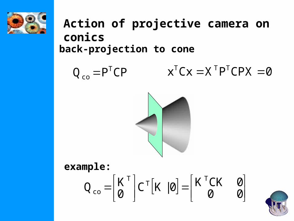
Action of projective camera on conics

back-projection to cone

CPPQ Tco 0CPXPXCxx TTT

000CKK0|KC

0KQ

TT

T

co

example:

Images of smooth surfaces

The contour generator is the set of points X on S at which rays are tangent to the surface. The corresponding apparent contour is the set of points x which are the image of X, i.e. is the image of

The contour generator depends only on position of projection center, depends also on rest of P

Action of projective camera on quadrics

back-projection to cone

TPPQC ** 0lPPQlQ T*T*T

The plane of for a quadric Q is camera center C is given by =QC (follows from pole-polar relation)

The cone with vertex V and tangent to the quadric Q isTT

CO (QV)(QV)-QV)QV(Q 0VQCO

The importance of the camera center

]C~

|[IR'K'P'C],|KR[IP

PKRR'K'P' -1

xKRR'K'PXKRR'K'XP'x' -1-1

-1KRR'K'HHx with x'

Moving the image plane (zooming)

xKK'0]X|[IK'x'0]X|K[Ix

1-

10

x~k)(1kIKK'H T

01-

100kIK

10x~kA

10x~A

10x~k)(1kI

K10

x~k)(1kIK'

TT0

T0

T0

T0

'/ ffk

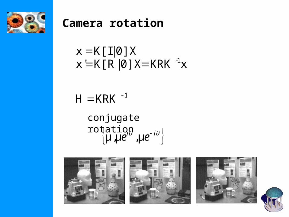
Camera rotation

xKRK0]X|K[Rx'0]X|K[Ix

1-

-1KRKH

conjugate rotation

ii ee μ,μμ,

Synthetic view

(i) Compute the homography that warps some a rectangle to the correct aspect ratio

(ii) warp the image

Planar homography mosaicing

close-up: interlacingcan be important problem!

Planar homography mosaicingmore examples

Projective (reduced) notation

T4

T3

T2

T1 )1,0,0,0(X,)0,1,0,0(X,)0,0,1,0(X,)0,0,0,1(X

T4

T3

T2

T1 )1,1,1(x,)1,0,0(x,)0,1,0(x,)0,0,1(x

dcdbda

000000

P

Tdcba ),,,(C 1111

Moving the camera center

motion parallax

epipolar line

What does calibration give?

xKd 1

0d0]|K[Ix

21-T-T

211-T-T

1

2-1-TT

1

2T

21T

1

2T

1

)xK(Kx)xK(Kx

)xK(Kx

dddd

ddcos

An image l defines a plane through the camera center with normal n=KTl measured in the camera’s Euclidean frame

The image of the absolute conic

KRd0d]C

~|KR[IPXx

mapping between ∞ to an image is given by the planar homogaphy x=Hd, with H=KR

image of the absolute conic (IAC)

1-T-1T KKKKω 1TCHHC

(i) IAC depends only on intrinsics(ii) angle between two rays(iii) DIAC=*=KKT

(iv) K (cholesky factorisation)(v) image of circular points

2T

21T

1

2T

1

ωxxωxx

ωxxcos

A simple calibration device

(i) compute H for each square (corners (0,0),(1,0),(0,1),(1,1))

(ii) compute the imaged circular points H(1,±i,0)T

(iii) fit a conic to 6 circular points(iv) compute K from through cholesky factorization

(= Zhang’s calibration method)

Orthogonality = pole-polar w.r.t. IAC

The calibrating conic

1T K1

11

KC

Vanishing points

λKdaλPDPAλPXλx

KdλKda limλ xlimvλλ

KdPXv

Vanishing lines

Orthogonality relation

2T

21T

1

2T

1

ωvvωvv

ωvvcos

0ωvv 2T

1

0lωl 2*T

1

Calibration from vanishing points and lines

Calibration from vanishing points and lines

Next class: Two-view geometryEpipolar geometry