WP/07/15

Mortality and Lifetime Income: Evidence from U.S. Social Security Records

James E. Duggan, Robert Gillingham,

and John S. Greenlees

© 2007 International Monetary Fund WP/07/15 IMF Working Paper Fiscal Affairs Department

Mortality and Lifetime Income: Evidence from U.S. Social Security Records

Prepared by James E. Duggan, Robert Gillingham, and John S. Greenlees1

Authorized for distribution by Gerd Schwartz January 2007

Abstract

This Working Paper should not be reported as representing the views of the IMF. The views expressed in this Working Paper are those of the author(s) and do not necessarily represent those of the IMF or IMF policy. Working Papers describe research in progress by the author(s) and are published to elicit comments and to further debate.

Studies of the empirical relationship between income and mortality often rely on data aggregated by geographic areas and broad population groups and do not distinguish disabled and nondisabled persons. We investigate the relationship between individual mortality and lifetime income with a large micro data base of current and former retired participants in the U. S. Social Security system. Logit models by gender and race confirm a negative relationship. Differences in age of death between low and high lifetime income are on the order of two to three years. Income-related mortality differences between blacks and whites are largest at low-income levels while gender differences appear to be large and persistent across income levels.

JEL Classification Numbers: C40, C67, D31, H20, I38 Keywords: Energy prices, subsidies, welfare distribution, household survey data

Authors’ E-Mail Addresses: james.duggan@do.treas.gov, rgillingham@imf.org; greenlees_j@bls.gov

1 James E. Duggan (U. S. Department of the Treasury) and John S. Greenlees (U. S. Bureau of Labor Statistics). The authors would like to thank Patricia Pollard for comments on an earlier version of this paper. The views expressed do not necessarily represent those of the Department of the Treasury of the Bureau of Labor Statistics.

2

Contents Page

I. Introduction ............................................................................................................................3

II. Previous Research on Income and Mortality ........................................................................4

III. Data and Variable Definitions .............................................................................................5

IV. Empirical Mortality Models ................................................................................................8 Retired Male Workers..................................................................................................10 Retired Female Workers ..............................................................................................10

V. How Large Are Income-Related Differences in Life Expectancy? ....................................12 Black and White Males................................................................................................12 Black and White Females ............................................................................................15

VI. Conclusion .........................................................................................................................18

References................................................................................................................................19 Tables 1. Characteristics of Retired Worker Beneficiaries ................................................................6 2. Estimated Mortality Hazard Models for Male Retired Workers 62+..............................10 3. Income and Work Years of Median Dual and Nondual Beneficiaries .............................11 4. Estimated Mortality Hazard Models for Female Retired Workers 62+ ...........................12 5. Median Ages of Death for Retired Workers Born in 1920...............................................13 6. Age-of-Death Differences at Constant Lifetime Incomes* ..............................................16 Figures 7. Deviations from Average Age of Death for Male Retired Workers...................................7 8. Distribution of Male Retirees by Trend in Earnings ..........................................................7 9. Cumulative Distribution of Age of Death of Male Retirees by Trend in Earnings............9 10. Cumulative Distribution of Lifetime Earnings for Retired Workers Born 1900–1942......9 11. Survivor Rates for White Male Retired Workers Born in 1920, Flat Earnings Profile....14 12. Survivor Rates for Black Male Retired Workers Born in 1920, Flat Earnings Profile ....14 13. Mortality Rates for 65-Year Old Men, by Earnings Levels .............................................15 14. Survivor Rates for White Female Non-Duals Born in 1920, Flat Earnings Profile .........17 15. Survivor Rates for Black Female Non-Duals Born in 1920, Flat Earnings Profile..........17

3

I. INTRODUCTION

The calculation of initial benefits in the U. S. Social Security system makes no attempt to reflect systematic differences across the population in mortality risk. Individuals of the same age with identical lifetime earnings profiles, and therefore with identical contribution amounts, receive the same initial benefit at retirement irrespective of differences in expected length of life. One consequence is that unintended redistribution can occur that depends on differences in life expectancy related to such factors as income, gender, and race. Milton Friedman pointed this out over thirty years ago, noting that higher income people have higher life expectancy and therefore receive benefits for a longer period of time (Friedman, 1972). Existing proposals to reform the Social Security system also generally ignore mortality risk. Even proposals for individual accounts often include annuitization provisions that could cause significant transfers from groups with higher mortality risk to those with lower risk (Brown, 2002). Economists, sociologists, demographers, and health professionals have all studied the relationship between life expectancy and socioeconomic status, and the literature has grown dramatically since the oft-cited study of Kitagawa and Hauser (1973). A common finding is that life expectancy is higher for higher income persons (Brown, 2002) and some research reports that the gap in mortality risk has been growing (Schalick, et al, 2000). Nevertheless, the literature in this area is relatively young and appropriate data are scarce. Most early research and some recent work rely on data aggregated by geographic areas and broad population groups, often categorizing people into income classes based on a single year of income. Such an approach cannot distinguish between populations that are temporarily and permanently in a certain income class, obscuring the distinct effects of permanent and transitory income. Moreover, most available databases do not distinguish disabled and nondisabled persons. Because disabled persons have far higher mortality than the general population (Zayatz, 1999) and their lifetime income is likely to be affected by their health status, combining the two populations may result in seriously misleading implications of the income-mortality relationship for Social Security calculations. In this paper we analyze empirically the seldom-investigated relationship between mortality and individual-specific socioeconomic status with data that largely avoid the aforementioned problems. Our data are administrative records from the Social Security Administration’s (SSA) 2002 one-percent Continuous Work History Sample (CWHS) that has actual covered earnings information spanning the period 1937 to 2002. The file contains month and year of death information for deceased persons covered by the Social Security program, along with race and gender indicators. Our data set also includes all of the benefit records from SSA’s Master Beneficiary Record (MBR) file that are associated with the CWHS records. The benefit records contain additional death information and allow us to separate the mortality experience of retired from disabled workers. Our results give strong empirical support to a negative relationship between individual lifetime income and mortality. For black and white males and females the difference in age of death between low and high lifetime income is on the order of two to three years. Workers with positively-trended earnings over their work life may live an additional six to eighteen months relative to those with declining earnings. Income-related mortality differences

4

between blacks and whites are largest at low-income levels, particularly for males, and narrow substantially at higher income levels. On the other hand, gender differences in mortality appear to be large and persistent across income levels. In Section II we briefly review previous research on income and mortality. In Section III we describe our data in detail, define variables of interest and illustrate mortality patterns that arise in our sample. In Section IV we develop logit models of the earnings-mortality relationship for retired-worker beneficiaries. In Section V we use estimated models to simulate survivor rates in order to further highlight the importance of lifetime income for mortality of retired workers. Section VI concludes with a brief discussion of the implications of our results for Social Security analyses.

II. PREVIOUS RESEARCH ON INCOME AND MORTALITY

The effect of income (or socioeconomic status generally) on mortality cannot be determined a priori. Higher income may be associated with higher mortality if the consumption of some goods and services that adversely affect health (red meats or skydiving, for example) increases with income. On the other hand, higher income may lead to increased consumption of goods and services that support health and prolonged life, such as shelter, protective clothing and medical care. The relationship between income and mortality is complex, but we would expect larger improvements in life expectancy to result from income increases at the lower end of the income distribution than at the upper end. Research on mortality has typically grouped people into socioeconomic strata in order to identify differences in mortality rates.2 Socioeconomic status has been proxied by education (e.g., Kitawaga and Hauser, 1973; Brown, 2002), family income (e. g., Kitawaga and Hauser, 1973; Hadley and Osei, 1982; Duleep, 1986; Rogers, 1992), and wealth (Menchik, 1993; Attanasio and Hoynes, 2000). Generally, these report a negative relationship between mortality and socioeconomic status. As pointed out by Brown (2002), however, socioeconomic status is captured imperfectly by education, family income, and wealth. Education may serve only as a rough proxy for lifetime earnings, while current family income is a poor measure of lifetime resources (low current income may simply reflect current poor health). Wealth is superior to education and current income in that respect though it may be correlated with health. In this paper we use a direct measure of lifetime resources (lifetime earnings) that avoids the drawbacks associated with other measures of socioeconomic status. Obviously, other factors also affect mortality. Mortality may vary by occupation, although most of the occupational differences in mortality are explained by income or education (Wilmoth and Dennis, 2006). Several researchers have assessed the comparative roles of race and other socioeconomic variables in determining death hazards, but agreement is lacking.

2Our references are not intended to be exhaustive of the literature on this topic. Kitawaga and Hauser (1973) thoroughly review early studies. Feinstein (1993) and Wilmoth and Dennis (2006) review more recent literature. Brown (2002) summarizes major findings from the literature on the socioeconomic status—mortality relationship.

5

Some authors find that black-white differences in mortality are fully explained by socioeconomic status while others find that socioeconomic status reduces, but does not eliminate black-white mortality differences (Wilmoth and Dennis, 2006). This paper provides new evidence on the income-race-mortality nexus.

III. DATA AND VARIABLE DEFINITIONS

Our primary data sources are the Social Security Administration’s 2002 one-percent Continuous Work History Sample (CWHS) and Master Beneficiary Record (MBR). The “active” portion of the CWHS (i.e., individuals with some covered earnings) is a historical record of Social Security earnings for over three million current or former workers in covered employment spanning the period 1937 to 2002. Each record has date of birth and race and sex indicators. When an individual files a claim for benefits based on her or his previous earnings history, SSA opens a claim account in the MBR file, the principal official record of historical benefit payments. If a worker attains beneficiary status and subsequently dies, the date of death is recorded in the MBR. Death information in the MBR is considered to be of very high quality (Aziz and Buckler, 1992). The administrative records have several advantages over data sets used in previous analyses of the determinants of mortality. The coverage is unparalleled, with the number of records many times larger than in any of the surveys with information on date of death. The CWHS has individual longitudinal information on lifetime earned income, as well as demographic information (age, race, sex), that is matched to mortality data. These data obviate aggregation or one-time measurement of the income variable that is of primary interest.3 The CWHS also has limitations for estimating mortality models. Most important for our purpose is that it contains information only on income earned in covered employment. Also, family background information that may impact on mortality rates is not included. Finally, race information in the administrative data permits only a three-way classification (blacks, whites, other).4 For empirical analysis we selected all retired-worker beneficiary records with birth years 1900 to 1942 who claimed benefits at age 62 or later. The birth year range allows us to observe a complete life for early cohorts and a nearly complete work life for later cohorts. Because our benefit/death information extends through 2004, the oldest observed age in our sample is 104. Accounting for edits and deletions for anomalous cases, our sample has nearly 550,000 observations.5 Some characteristics of our sample are shown in Table 1. 3Hoyert, Singh, and Rosenberg (1995) summarize the principal data sets available to evaluate mortality and socioeconomic status. 4Since 1980, race information collected in the administrative records has expanded to include five race/ethnic responses: White (not Hispanic), Black (not Hispanic), Hispanic, Asian or Pacific Islander, and American Indian or Alaskan Native. Prior to 1980, only the three-way classification was allowed. The vast majority of records analyzed in this paper would not, of course, benefit from the expanded classification. 5One anomaly in our sample occurs with records that show no recent work activity, no benefits, insufficient quarters of coverage for benefit eligibility, and no death information. These records accounted for less than nine percent of the sample before edits. The vast majority of these records are missing death information in our file

(continued…)

6

Table 1. Characteristics of Retired Worker Beneficiaries

Females Males

Category Sample White Black Other White Black Other

Sample (%) 100.0 38.5 3.7 1.1 50.6 4.4 1.7 Dead (%) 49.0 43.6 45.4 24.4 54.2 59.0 37.5 Median Age of Death 77.0 80.0 78.0 79.0 76.0 75.0 77.0 Median Lifetime Earnings* 517,158 269,574 236,917 233,227 921,999 476,051 413,088

Source: Authors' calculations based on CWHS and MBR (sample=548,681).* Sum over ages 35 through 60 in 2005 dollars.

Nearly half of retired-worker beneficiaries in our sample have died. The percentages are higher for males than females and higher for blacks than whites. For retired-worker beneficiaries who have already died, the median female lived about four years longer than the median male, and the median white lived about one to two years longer than the median black. Lifetime earnings are measured for each individual as the sum of real earnings (2005 dollars) over ages 35 to 60 (ages 37 to 60 and 36 to 60 for birth years 1900 and 1901, respectively).6 As seen in Table 1, males earned more than females and whites earned more than blacks. The relationship between age of death and lifetime earnings for deceased male retired workers in our sample is illustrated in Figure 1 (a similar, but less steeply-sloped pattern arises for females). The figure shows three five-year birth cohorts, selected to represent patterns across the birth cohorts in our sample, with each five-year birth cohort sorted into deciles of lifetime earnings. The figure plots the differences between the average age of death in each earnings class and the average age of death across the earnings classes, thereby adjusting for scale differences across birth cohorts. For the 1910–14 birth cohorts, difference in age of death between highest and lowest earnings deciles is about twenty months; for the 1920–24 cohorts, the difference is about a fifteen months and about eight months for the most recent cohorts. The figure clearly depicts a positive relationship between lifetime earnings and length of life.

due to state agreements with SSA on the use of death reports. We deleted these records on the grounds that their exclusion would be less distorting than their inclusion. The exclusion has no effect on our later econometric estimates that focus on beneficiaries. 6Earned income in the CWHS consists of lump-sum taxable earnings for 1937 to 1950, annual taxable earnings from 1951 to 1977, and total (uncapped) earnings from 1978 to 2002. We use these earnings data to develop a summary measure of real lifetime earnings following three adjustments to the data: (1) we prorated the 1937 to 1950 lump-sum under the assumption that, between the reported first and last years of employment prior to 1951, earnings grew at one percent per year of age beyond the economy-wide growth in wages for males and at one-half percent for females, using the average annual earnings between 1937 and 1950 from Myers (1993); (2) for individuals who earned the taxable maximum during years 1937-1980, we imputed earnings above the maximum using a Tobit model of earnings under the assumption that earnings are lognormally distributed; (3) earnings (actual or imputed) in each year were indexed to 2005 using the Consumer Price Index.

7

Figure 1. Deviations from Average Age of Death for Male Retired Workers

-1.00

-0.75

-0.50

-0.25

0.00

0.25

0.50

0.75

1.00

1 2 3 4 5 6 7 8 9 10

Lifetime Earnings Class

1910-14

1920-24 1930-34

Average Age of Death by Birth Year:1910-14: 77.91920-24: 74.81930-34: 68.1

Figure 2. Distribution of Male Retirees by Trend in Earnings

0%

10%

20%

30%

40%

50%

60%

70%

80%

1910-14 1915-19 1920-24 1925-29 1930-34 1935-39

Birth Cohort

Rising Level Declining

8

Later we will examine in some detail the importance of this measure of “permanent income” for mortality outcomes. We are also interested in the relationship between the pattern of earnings over the work cycle and life expectancy. Many workers exhibit low adherence to the workforce due to limited skills or poor health while others, for similar reasons, may have steady workforce attachment but achieve little progress in real earnings. On the other hand, workers who continue to improve their earnings positions are likely to be more skilled, in better health, and generally more productive. The latter group may also have longer life expectancies. We attempt to capture these effects by classifying workers according to whether the trend in their real earnings over prime working ages has risen, remained flat, or fallen.7 Specifically, consider an individual worker’s average real earnings during the three equal age periods 37 to 44, 45 to 52, and 53 to 60 and label the periods AE1, AE2, and AE3, respectively. The trend in a worker’s real earnings can be measured as:

Trend = (AE3 – AE1)/(AE1 + AE3).

We classify workers according to earnings trend as follows:

Declining if Trend < -1/9,

Flat if -1/9 ≤ Trend ≤ 1/9,

Rising if Trend > 1/9. Figure 2 shows a steady decline in the percentage of male retired workers with a rising Trend and a steady rise in the percentage with a declining Trend. A similar but more modest change in Trend has occurred for females. Figure 3 illustrates the relationship between cumulative age of death and the trend in earnings for deceased male retired workers. The age-of-death distribution for male workers with a declining earnings trend lies above the distribution for workers with rising or flat trends. The difference in median age of death between those with rising trends and those with declining trends is about four years.

IV. EMPIRICAL MORTALITY MODELS

In this section we estimate mortality models for white and black male and female retired workers. The unit of observation is an individual year of a worker’s life and the dependent variable is the binary realization of the “hazard rate,” indicating whether or not death took place in that year, given that the individual was alive at the end of the previous year. We estimate the hazard directly using the logit probability model so that variables with positive coefficients are associated with higher death rates and shorter expected lifetimes. Explanatory variables in our models include (log of) real lifetime earnings, age, year of birth,

7The earnings classification scheme described below is based on work performed on the 1972 CWHS and reported in the Committee on Finance (1976), pp. 75–81.

9

Figure 3. Cumulative Distribution of Age of Death of Male Retirees by Trend in Earnings

0%

25%

50%

75%

100%

62 64 66 68 70 72 74 76 78 80 82 84 86 88 90 92 94

Age of Death

Declining Trend

Rising Trend

Flat Trend

Figure 4. Cumulative Distribution of Lifetime Earnings for Retired Workers Born 1900–1942

0%

25%

50%

75%

100%

40 200 360 520 680 840 1,000 1,160 1,320 1,480 1,640 1,800 1,960 2,120

Thousands of 2005 Dollars

White Males

Black Males

White Females

Black Females

10

and indicators of rising and flat earnings trends (declining trend is omitted). In this specification, real earnings will vary both across and within cohorts.8 The birth year variable is designed to capture trends in mortality unrelated to the growth in real income over time. The earnings variable is specified as a cubic polynomial in order to allow flexibility in the way earnings affect mortality. Retired Male Workers

Table 2 displays our parameter estimates for male retired workers. Most coefficients are highly significant, reflecting in part the large sample sizes.9 The probability of death rises with age and falls with cohort birth year. An additional year of age increases the odds of death by nine to ten percent for retired male workers.10 The probability of death falls for more recent birth cohorts, presumably reflecting trends in health care and nutrition, although the estimated coefficients are not statistically significant for black retirees. For white and black males born in 1930, for example, the odds of death are sixteen and five percent lower, respectively, than for retirees born in 1920, ceteris paribus. The trend in earnings also has a negative effect on mortality. Relative to a declining trend, a rising trend reduces the odds of mortality by about twenty percent and a flat trend reduces the odds by ten to thirteen percent. In each case, mortality is significantly negatively related to the log of lifetime earnings, a result that we explore further below. Retired Female Workers

For many female workers, the primary source of earned income may not be their own earnings but that of their spouses. In these cases, spousal earnings, in addition to a worker’s own earnings, may better capture the effects of lifetime income on mortality. Unfortunately, Social Security records do not identify marital status per se so that pairing all married workers is not possible. Yet, the records do identify beneficiary couples when an individual receives a benefit based on their own earnings history and an 8As noted above, the Consumer Price Index is used to deflate nominal earnings. Duggan and Gillingham (1999) examine potential errors in that index series and the potential impact of those errors on Social Security finances. 9The basic sample consists of 277,571 while males and 24,160 black males. In person-year format, there are over 3.8 million white-male observations and over 317 thousand black-male observations. 10The logit parameters measure the marginal impact of independent variables on the log odds of death; i.e., on ln[p/(1-p)] where p is the probability of death. In percentage terms, the effect of an additional year of age on the odds of death for retired white male workers, for example, is given by 100(e.0952 – 1).

Table 2. Estimated Mortality Hazard Models for

Male Retired Workers 62+

Variable White males Black males

Intercept - 9.991 - 9.400(0.000) (-0.142)

Age 0.095 0.088(-1.092) (-0.001)

Birth Year - 0.017 - 0.006(-0.994) (-0.001)

–– Lifetime Earnings (LE) ––

LE - 0.341 - 0.406(-0.667) (-0.064)

LE2 0.067 0.079(-1.083) (-0.010)

LE3 - 0.003 - 0.004(-0.996) (-0.000)

––– Trend in Earnings –––

Rising - 0.214 - 0.195(-0.823) (-0.022)

Flat - 0.101 - 0.129(-0.879) (-0.029)

* Estimated standard errors in parentheses

11

auxiliary benefit based on the earnings of their current or former spouse. These dual beneficiary cases are common among female retirees—about half of female retired workers are dual beneficiaries.11 For these cases, we are able to match the actual earnings history of the (current or former) spouse with the beneficiary’s record and thereby include a second known source of income in the female mortality model.12

Table 3. Income and Work Years of Median Dual and Nondual Beneficiaries

Duals (N=94,945) Nonduals (N=123,979)

White Black

own spouse own spouse

Median lifetime income* 150,749 1,013,750 130,029 501,740 420,491 310,227Years with posit ive income 20 23 28

Source: Authors' calculations based on CWHS and MBR.*Lifetime income is the sum of real earnings (2005 dollars) over ages 35-60.

White Black

Female dual beneficiaries are current or former retired-worker beneficiaries who also received either a spousal or widow’s benefit based on the earnings of a current or former spouse. Female nonduals are current or former retired-worker beneficiaries with no auxiliary benefit.13 Duals and nonduals differ considerably in their income and work experience, as shown in Table 3. The median earner nondual white female had nearly three times the earnings of the median dual white female; for blacks, the ratio was nearly two and a half to one. Duals had six to eight years fewer years of market work than nonduals due at least in part to child-rearing. Finally, the median-earner spouse of white female duals earned nearly seven times that of the dual whereas the median-earner spouse of black females had nearly four times the earnings of the dual (about five percent of black female retired workers are duals). Table 4 presents parameter estimates for mortality models for the nondual and dual retired female workers. Own lifetime earnings has a significantly negative effect on mortality for both dual and nondual females. For white female duals, lifetime earnings of their spouses

11Some unknown proportion of female retired worker beneficiaries may be married,but not receive an auxiliary benefit because their own benefit exceeds the auxiliary benefit amount. For those individuals, benefit records do not reveal marital status. Male retirees may also be dual beneficiaries but the number is very small. 12The lifetime income of spouses were computed in the same manner as for the primary worker, described in section III. That is, we first impute above-cap earnings for those earning the maximum and then sum their real earnings over ages 35-60. 13For the empirical analysis, we have 123,979 nonduals and 94,945 dual beneficiaries (about 95 percent of the white and black females represented in Table 1. We omitted about 10 percent of duals who were mainly divorced wives and widows who were not the primary claimants on a dual account.

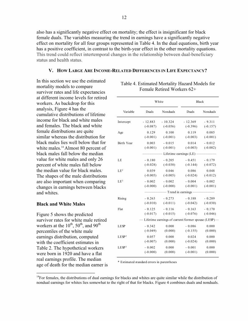
12

also has a significantly negative effect on mortality; the effect is insignificant for black female duals. The variables measuring the trend in earnings have a significantly negative effect on mortality for all four groups represented in Table 4. In the dual equations, birth year has a positive coefficient, in contrast to the birth-year effect in the other mortality equations. This trend could reflect intertemporal changes in the relationship between dual-beneficiary status and health status.

V. HOW LARGE ARE INCOME-RELATED DIFFERENCES IN LIFE EXPECTANCY?

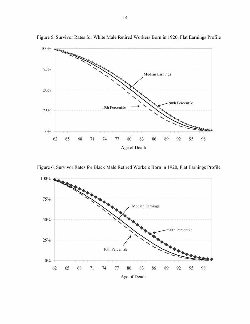
In this section we use the estimated mortality models to compare survivor rates and life expectancies at different income levels for retired workers. As backdrop for this analysis, Figure 4 has the cumulative distributions of lifetime income for black and white males and females. The black and white female distributions are quite similar whereas the distribution for black males lies well below that for white males.14 Almost 80 percent of black males fall below the median value for white males and only 26 percent of white males fall below the median value for black males. The shapes of the male distributions are also important when comparing changes in earnings between blacks and whites. Black and White Males

Figure 5 shows the predicted survivor rates for white male retired workers at the 10th, 50th, and 90th percentiles of the white male earnings distribution, computed with the coefficient estimates in Table 2. The hypothetical workers were born in 1920 and have a flat real earnings profile. The median age of death for the median earner is 14For females, the distributions of dual earnings for blacks and whites are quite similar while the distribution of nondual earnings for whites lies somewhat to the right of that for blacks. Figure 4 combines duals and nonduals.

Table 4. Estimated Mortality Hazard Models for Female Retired Workers 62+

White Black

Variable Duals Nonduals Duals Nonduals

Intercept - 12.883 - 10.324 - 12.369 - 9.311(-0.087) (-0.056) (-0.396) (-0.157)

Age 0.129 0.100 0.119 0.085(-0.001) (-0.001) (-0.003) (-0.001)

Birth Year 0.003 - 0.015 0.014 - 0.012(-0.001) (-0.001) (-0.003) (-0.002)

––––––––––– Lifetime earnings (LE) –––––––––––

LE - 0.180 - 0.205 - 0.451 - 0.179(-0.028) (-0.030) (-0.144) (-0.072)

LE2 0.039 0.046 0.086 0.048(-0.005) (-0.005) (-0.024) (-0.012)

LE3 - 0.002 - 0.002 - 0.004 - 0.002(-0.000) (-0.000) (-0.001) (-0.001)

–––––––––––– T rend in earnings ––––––––––––

Rising - 0.263 - 0.273 - 0.188 - 0.289(-0.010) (-0.011) (-0.042) (-0.030)

Flat - 0.125 - 0.116 - 0.163 - 0.170(-0.017) (-0.015) (-0.076) (-0.046)

–– Lifetime earnings of current/former spouse (LESP) ––

LESP - 0.342 0.000 - 0.086 0.000(-0.049) (0.000) (-0.155) (0.000)

LESP2 0.057 0.000 0.024 0.000(-0.007) (0.000) (-0.024) (0.000)

LESP3 - 0.002 0.000 - 0.001 0.000(-0.000) (0.000) (-0.001) (0.000)

* Estimated standard errors in parentheses

13

80.3 years (Table 5). For the low and higher earners, the median ages of death are 78.8 and 81.6, respectively. For these workers, there is an approximately thirty-three month difference in age of death between the lowest and highest deciles. The median ages of death for hypothetical workers with a rising earnings trend (also presented in Table 5) are about a year higher at each percentile.

Table 5. Median Ages of Death for Retired Workers Born in 1920

Flat earnings trend Rising earnings trend

Retirees 10th Median 90th90th-10th(months) 10th Median 90th

90th-10th(months)

MalesWhite 78.8 80.3 81.6 33 79.8 81.3 82.6 33 Black 76.8 77.8 80.3 42 77.3 78.3 80.8 42

Female NondualsWhite 82.1 83.1 84.3 26 83.5 84.5 85.8 27 Black 81.1 82.5 84.8 45 82.3 83.8 86.1 45

Female DualsWhite

Own earnings 84.1 85.0 86.4 28 85.1 86.1 87.5 29 Husband's earnings 84.6 85.0 85.4 10 85.7 86.1 86.4 9

BlackOwn earnings 82.1 83.3 85.9 46 83.0 84.3 86.9 47 Husband's earnings 83.2 83.3 83.5 4 84.2 84.3 84.5 4

Figure 6 has survivor rates for similarly defined hypothetical black male retired workers. The median age of death for the black median-earner retired worker is 77.8, two and a half years lower than that of the white median earner. For low and high earners, the median ages of death are 76.8 and 80.3, respectively. The age-of-death difference between the lowest and highest earners is over three years (forty-two months). For black workers, a positive trend results in about a half year greater life expectancy. Differences in the black-white earnings distributions are large enough to make mortality comparisons at the top of the white male distribution infeasible. For example, the black male survivor function doesn’t generate a median age of death of 80.3, the median age of death for median-earner white males, until about the 96th percentile of the black male earnings distribution. On the other hand, points along the black earnings distribution are feasible for whites, even if incomplete. At the 10th and 90th percentile values of the black male distribution, the median ages of death for white males are 79.0 and 81.3, respectively, compared to 76.8 and 80.3 for black males. This indicates that the largest differences in mortality between black and white males occur at low earnings levels with the differences narrowing as earnings levels rise. Improvements in mortality at the high end of the white male distribution are outside the range of black male earnings.

14

Figure 5. Survivor Rates for White Male Retired Workers Born in 1920, Flat Earnings Profile

0%

25%

50%

75%

100%

62 65 68 71 74 77 80 83 86 89 92 95 98

Age of Death

90th Percentile

Median Earnings

10th Percentile

Figure 6. Survivor Rates for Black Male Retired Workers Born in 1920, Flat Earnings Profile

0%

25%

50%

75%

100%

62 65 68 71 74 77 80 83 86 89 92 95 98

Age of Death

90th Percentile

Median Earnings

10th Percentile

15

An alternative illustration of the black-white income-mortality gap is provided in Figure 7. The figure shows mortality rates by earnings levels for 65-year-old black and white males. The rates decline as earnings levels increase. Differences in the rates decline steadily, particularly at lower earnings levels. The mortality rate difference begins at about 0.5 percentage points at the lowest income level and falls by a third at about $1.4 million in lifetime earnings, which occurs at the 95th percentile of the black male earnings distribution.

Figure 7. Mortality Rates for 65-Year Old Men, by Earnings Levels

1.3%

1.7%

2.1%

2.5%

2.9%

80 200 320 440 560 680 800 920 1040 1160 1280 1400

Thousands of Dollars

Blacks

Whites

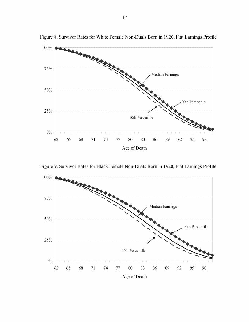
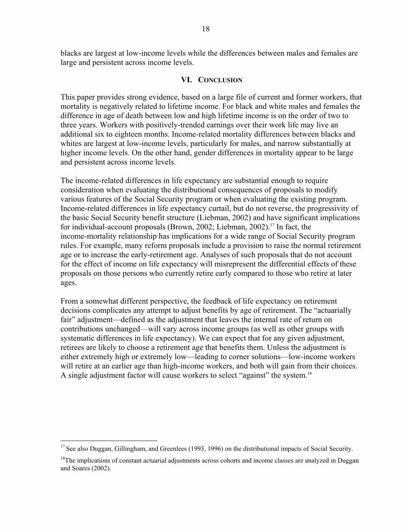
Black and White Females

We define hypothetical female workers in a similar way to that used for males. For nonduals, survivor profiles are shown in Figures 8 and 9 for white and black females, respectively. For white nonduals, the median age of death ranges from 82.1 to 84.3 between the 10th and 90th percentiles of their lifetime earnings distribution, a difference of 26 months (Table 5). For black nonduals, the difference in the median age of death is larger—45 months. For black and white nonduals, a positive earnings trend adds over a year to life expectancy. For duals there are two sources of lifetime income variation—own and spouses—and we construct survivor profiles by allowing one or the other to vary while holding one to its median value.15 The results are summarized in Table 5. Higher own lifetime earnings has a

15Allowing both to vary at the same time would provide the largest income-related differences in life expectancy so our simulations are conservative in this respect. Because we found little empirical relationship between own and spouse’s lifetime earnings, we allow the income variables to vary independently.

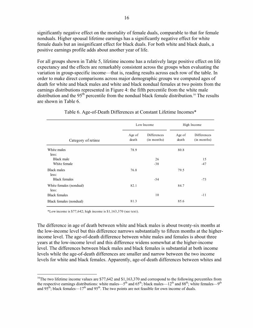
16

significantly negative effect on the mortality of female duals, comparable to that for female nonduals. Higher spousal lifetime earnings has a significantly negative effect for white female duals but an insignificant effect for black duals. For both white and black duals, a positive earnings profile adds about another year of life. For all groups shown in Table 5, lifetime income has a relatively large positive effect on life expectancy and the effects are remarkably consistent across the groups when evaluating the variation in group-specific income—that is, reading results across each row of the table. In order to make direct comparisons across major demographic groups we computed ages of death for white and black males and white and black nondual females at two points from the earnings distributions represented in Figure 4: the fifth percentile from the white male distribution and the 95th percentile from the nondual black female distribution.16 The results are shown in Table 6.

Table 6. Age-of-Death Differences at Constant Lifetime Incomes*

Low Income High Income

Category of retireeAge ofdeath

Differences (in months)

Age ofdeath

Differences (in months)

White males 78.9 80.8less:

Black male 26 15White female -38 -47

Black males 76.8 79.5less:

Black females -54 -73

White females (nondual) 82.1 84.7less:

Black females 10 -11

Black females (nondual) 81.3 85.6

*Low income is $77,642; high income is $1,163,370 (see text). The difference in age of death between white and black males is about twenty-six months at the low-income level but this difference narrows substantially to fifteen months at the higher-income level. The age-of-death difference between white males and females is about three years at the low-income level and this difference widens somewhat at the higher-income level. The differences between black males and black females is substantial at both income levels while the age-of-death differences are smaller and narrow between the two income levels for white and black females. Apparently, age-of-death differences between whites and

16The two lifetime income values are $77,642 and $1,163,370 and correspond to the following percentiles from the respective earnings distributions: white males—5th and 65th; black males—12th and 88th; white females—9th and 95th; black females—17th and 95th. The two points are not feasible for own income of duals.

17

Figure 8. Survivor Rates for White Female Non-Duals Born in 1920, Flat Earnings Profile

0%

25%

50%

75%

100%

62 65 68 71 74 77 80 83 86 89 92 95 98

Age of Death

Median Earnings

10th Percentile

90th Percentile

Figure 9. Survivor Rates for Black Female Non-Duals Born in 1920, Flat Earnings Profile

0%

25%

50%

75%

100%

62 65 68 71 74 77 80 83 86 89 92 95 98

Age of Death

90th Percentile

Median Earnings

10th Percentile

18

blacks are largest at low-income levels while the differences between males and females are large and persistent across income levels.

VI. CONCLUSION

This paper provides strong evidence, based on a large file of current and former workers, that mortality is negatively related to lifetime income. For black and white males and females the difference in age of death between low and high lifetime income is on the order of two to three years. Workers with positively-trended earnings over their work life may live an additional six to eighteen months. Income-related mortality differences between blacks and whites are largest at low-income levels, particularly for males, and narrow substantially at higher income levels. On the other hand, gender differences in mortality appear to be large and persistent across income levels. The income-related differences in life expectancy are substantial enough to require consideration when evaluating the distributional consequences of proposals to modify various features of the Social Security program or when evaluating the existing program. Income-related differences in life expectancy curtail, but do not reverse, the progressivity of the basic Social Security benefit structure (Liebman, 2002) and have significant implications for individual-account proposals (Brown, 2002; Liebman, 2002).17 In fact, the income-mortality relationship has implications for a wide range of Social Security program rules. For example, many reform proposals include a provision to raise the normal retirement age or to increase the early-retirement age. Analyses of such proposals that do not account for the effect of income on life expectancy will misrepresent the differential effects of these proposals on those persons who currently retire early compared to those who retire at later ages. From a somewhat different perspective, the feedback of life expectancy on retirement decisions complicates any attempt to adjust benefits by age of retirement. The “actuarially fair” adjustment—defined as the adjustment that leaves the internal rate of return on contributions unchanged—will vary across income groups (as well as other groups with systematic differences in life expectancy). We can expect that for any given adjustment, retirees are likely to choose a retirement age that benefits them. Unless the adjustment is either extremely high or extremely low—leading to corner solutions—low-income workers will retire at an earlier age than high-income workers, and both will gain from their choices. A single adjustment factor will cause workers to select “against” the system.18

17 See also Duggan, Gillingham, and Greenlees (1993, 1996) on the distributional impacts of Social Security. 18The implications of constant actuarial adjustments across cohorts and income classes are analyzed in Duggan and Soares (2002).

19

References

Attanasio, Orazio, and Hilary Williamson Hoynes, 2000, “Differential Mortality and Wealth Accumulation,” Journal of Human Resources, Vol. 35, No. 1 (Winter), pp. 1–29.

Aziz, Faye, and Warren Buckler, 1992, “The Status of Death Information in Social Security Administration Files,” paper presented at the Annual Meeting of the American Statistical Association, Boston.

Brown, Jeffrey, 2002, “Differential Mortality and the Value of Individual Account Retirement Annuities,” in The Distributional Aspects of Social Security and Social Security Reform, ed. by M. Feldstein and J. Liebman (Chicago: University of Chicago Press).

Committee on Finance of the U. S. Senate and the Committee on Ways and Means of the U. S. House of Representatives, 1976, Report of the Consultant Panel on Social Security to the Congressional Research Service, (August), pp. 75–81.

Duggan, James. E., and Robert Gillingham, 1999, “The Effect of Errors in the CPI on Social Security Finances,” Journal of Business and Economic Statistics, Vol. 17, No. 2 (April), pp. 161–69.

––––––, Robert Gillingham, and John Greenlees, 1993, “The Returns Paid to Early Social Security Cohorts,” Contemporary Policy Issues, (October), pp. 1–13.

———, 1996, “Distributional Effects of Social Security: The Notch Issue Revisited,” Public Finance Quarterly, Vol. 24, No. 3 (July), pp. 349–70.

Duggan, James. E., and Christopher Soares, 2002, “Actuarial Nonequivalence in Early and Delayed Social Security Benefit Claims,” Public Finance Review, Vol. 30, No. 3 (May), pp. 188–207.

Duleep, Harriet, 1986, “Measuring the Effect of Income on Adult Mortality Using Longitudinal Administrative Record Data,” The Journal of Human Resources, XXI(2) (Spring), pp. 238–51.

Feinstein, Jonathan, 1993, “The Relationship Between Socioeconomic Status and Health: A Review of the Literature,” The Milbank Quarterly, Vol. 71, No. 2, pp. 279–322.

Friedman, Milton, 1972, “Second Lecture,” in Social Security: Universal or Selective? ed. by W. Cohen and M. Friedman (Washington: American Enterprise Institute).

Hadley, Jack H., and Anthony O. Osei, 1982, “Does Income Affect Mortality? An Analysis of the Effects of Different Types of Income on Age/Sex/Race-Specific Mortality Rates in the United States,” Medical Care, XX (9) (September), pp. 901–14.

20

Hoyert, Donna, Gopal Singh, and Harry Rosenberg, 1995, “Sources of Data on Socioeconomic Differential Mortality in the United States,” Journal of Official Statistics, Vol. 11, No. 3, pp. 233–60.

Kitagawa, Evelyn, and Philip Hauser, 1973, Differential Mortality in the U. S.: A Study of Socioeconomic Epidemiology (Cambridge: Harvard University Press).

Liebman, Jeffrey, 2002, “Redistribution in the Current U. S. Social Security System,” The Distributional Aspects of Social Security and Social Security Reform, ed. by M. Feldstein and J. Liebman (Chicago: University of Chicago Press).

Menchik, Paul, 1993, “Economic Status as a Determinant of Mortality Among Nonwhite and White Older Males: Or, Does Poverty Kill?” Population Studies, Vol. 47, pp. 427–36.

Rogers, Richard G., 1992, “Living and Dying in the U. S. A.: Sociodemographic Determinants of Death Among Blacks and Whites,” Demography, 29(2) (May), pp. 287–303.

Schalick, Lisa Miller, and others, 2000, “The Widening Gap in Death Rates among Income Groups in the United States from 1967 to 1986,” International Journal of Health Services, 30/1, pp. 13–26.

Wilmoth, John R., and Mike Dennis, 2006, “Social differences in older adult mortality in the United States: Questions, Data, Methods, and Results,” forthcoming in Human Longevity, Individual Life Duration, and the Growth of the Oldest-Old Population, ed. by Jean-Marie Robine and others (Oxford, U.K.: Oxford University Press).

Zayatz, Tim, 1999, Social Security Disability Program Worker Experience, Actuarial Study No. 114 (Baltimore: Office of the Actuary, Social Security Administration).