mos unit ii

Mechanics of Solids (NME-302) Unit-II

Unit-II

UNIT –II

Stresses in Beams:

2.1 Pure Bending

2.2 Normal Stresses in Beams

2.3 Shear Stresses in Beams due to transverse and axial loads

2.4 Composite Beams

Deflection of Beams:

2.5 Equation of Elastic Curve

2.6 Cantilever and Simply Supported Beams

2.7 Macaulay’s method

2.8 Area moment method

2.9 Fixed and Continuous Beams

Torsion:

2.10 Combined Bending & Torsion of Solid & Hollow Shafts

2.11 Torsion of Thin Walled Tubes


Unit-II

Stresses in Beams

Assumptions in Theory of Simple Bending:

A relationship is developed between the bending moment on a section of a beam and the stress developed in

the beam section. To achieve a simple relationship between bending moment and stress following

assumptions are taken:

1. The beam is initially straight, that is, no initial curvature in the beam.

2. The material of the beam is homogeneous, that is, it possesses same physical properties throughout the

volume.

3. The material of the beam is isotropic, that is, its elastic constants do not vary throughout its volume.

4. Young’s modulus of the material in tension Et is the same as Young’s modulus in compression EC.

5. The elastic limit of the material σe is not exceeded, that is, stresses in the material at any section at any layer

do not exceed σe, in other words when bending moment is removed from the beam, it comes back to its

original shape and original dimensions.

6. Each layer of the beam is independent to contract or to extend irrespective of the layers above or below it,

that is, whole beam acts as a pack of cards or sheets.

7. The beam section is symmetrical about the plane of bending, as Fig. 8.1 shows plane of bending and section

symmetrical about plane of bending.

8. Transverse sections which are plane before bending remain plane after bending and only the direction of

plane is changed.

Figure 8.2(a) shows a plane abcd in a straight beam which has not bent. After the application of bending

moment, plane abcd has changed its position to a′b′c′d′, that is, it has rotated by an angle f as shown in Fig.

8.2(b).

Theory of Simple Bending:

Consider that a small length dx of the beam is subjected to bending moment M as shown in Fig. After the

beam bends, the element dx also bends and the shape is changed to a′b′c′d′ such that a′b′ < ab and c′d′ > cd,

that is, the upper length of the element is decreased and the lower length of the element is increased. So in the

upper layer ab, there is a compressive strain and in the lower layer cd, there is a tensile strain. Strain changes

from negative to positive from top layer to bottom layer as shown in the figure. Therefore, when there is a


Unit-II

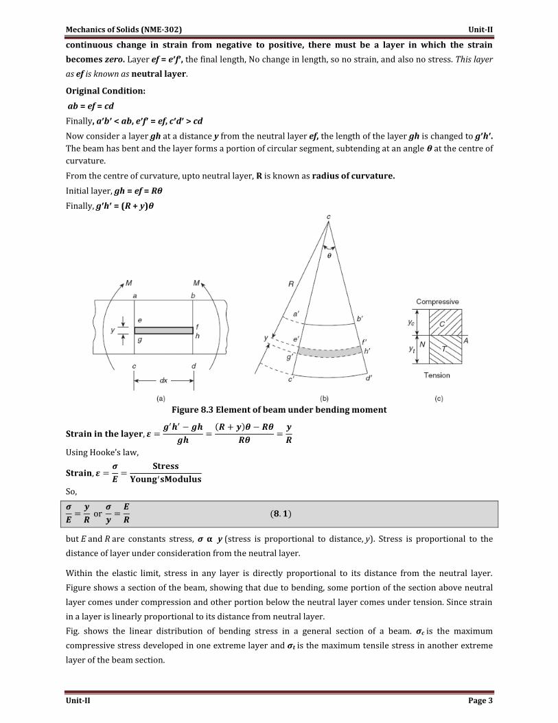
continuous change in strain from negative to positive, there must be a layer in which the strain

becomes zero. Layer ef = e′f′, the final length, No change in length, so no strain, and also no stress. This layer

as ef is known as neutral layer.

Original Condition:

ab = ef = cd

Finally, a′b′ < ab, e′f′ = ef, c′d′ > cd

Now consider a layer gh at a distance y from the neutral layer ef, the length of the layer gh is changed to g′h′.

The beam has bent and the layer forms a portion of circular segment, subtending at an angle θ at the centre of

curvature.

From the centre of curvature, upto neutral layer, R is known as radius of curvature.

Initial layer, gh = ef = Rθ

Finally, g′h′ = (R + y)θ

Figure 8.3 Element of beam under bending moment

Using Hooke’s law,

So,

but E and R are constants stress, σ α y (stress is proportional to distance, y). Stress is proportional to the

distance of layer under consideration from the neutral layer.

Within the elastic limit, stress in any layer is directly proportional to its distance from the neutral layer.

Figure shows a section of the beam, showing that due to bending, some portion of the section above neutral

layer comes under compression and other portion below the neutral layer comes under tension. Since strain

in a layer is linearly proportional to its distance from neutral layer.

Fig. shows the linear distribution of bending stress in a general section of a beam. σc is the maximum

compressive stress developed in one extreme layer and σt is the maximum tensile stress in another extreme

layer of the beam section.


Unit-II

Figure 8.4 Linear stress distribution

Neutral Axis:

Consider any section of the beam as shown in Fig. 8.5, stress in layer ab

or,

Force in a small element of area dA,

dP = σ dA

Total force, on section,

We have not applied any force, but we have applied only moment M.

NA = neutral axis, h = arm of couple

Note that the first moment of any area is zero only about its centroidal axis; therefore, neutral axis of

the beam passes through the centroid G of the section.

Moreover, Pc = net force on compression side of the section.

Pt = net force on tension side of section.

Pc = Pt, both these equal and opposite forces constitute a couple of arm h as shown.

Pc × h = Pt × h = moment applied on the beam section.

Moment of Resistance:

We have considered a small element of area dA at a distance of y from neutral layer neutral axis.

Force on the area, dP = σ dA

Moment of force dP, about neutral layer

Total moment of resistance,

Figure 8.5


Unit-II

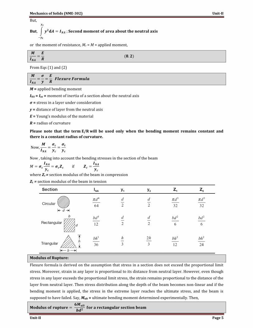
But,

or the moment of resistance, Mr = M = applied moment,

From Eqs (1) and (2)

M = applied bending moment

INA = Ixx = moment of inertia of a section about the neutral axis

σ = stress in a layer under consideration

y = distance of layer from the neutral axis

E = Young’s modulus of the material

R = radius of curvature

Please note that the term E/R will be used only when the bending moment remains constant and

there is a constant radius of curvature.

Now , taking into account the bending stresses in the section of the beam

where Zc = section modulus of the beam in compression

Zt = section modulus of the beam in tension

Modulus of Rupture:

Flexure formula is derived on the assumption that stress in a section does not exceed the proportional limit

stress. Moreover, strain in any layer is proportional to its distance from neutral layer. However, even though

stress in any layer exceeds the proportional limit stress, the strain remains proportional to the distance of the

layer from neutral layer. Then stress distribution along the depth of the beam becomes non-linear and if the

bending moment is applied, the stress in the extreme layer reaches the ultimate stress, and the beam is

supposed to have failed. Say, Mult = ultimate bending moment determined experimentally. Then,


Unit-II

where b = breadth of the rectangular section, d = depth of the rectangular section.

The flexure formula is not valid if the stresses go beyond proportional limit stress. The theoretical value of

the fracture stress obtained by flexure formula using ultimate bending moment is known as the modulus of

rupture.

Beams of Uniform Strength:

To achieve a beam of uniform strength for the purpose of saving in material cost of the beam, the term M/Z,

that is, ratio of bending moment and section modulus Z is to be maintained constant either (a) by varying the

breadth of the beam or (b) by varying the depth of the beam. Maximum stress in a section under bending is

developed at extreme edges of the section. This maximum skin stress is maintained constant.

In the formula

For a rectangular section, Z = bd2/6, as shown in Fig. 8.19.

So,

Considering the example of a simple supported beam with a concentrated

load at the centre, Fig. 8.20 shows the BM diagram in portion AB of

the beam, the bending moment at distance x from end A.

If breadth is also varied linearly from zero at A to bx at distance x, then

A constant term σ is the maximum tensile/compressive stress at extreme edges of a rectangular section.

Similarly in the case of a cantilever, with a concentrated load at the free end, as shown in Fig. 8.21.

Bending moment at a distance x from free end A,

Mx = Wx

where B is width at fixed end, d depth remains

constant throughout the length of the beam.

Variation of Depth (Breadth remains constant):

Simply supported beam

Figure 8.19 Rectangular section

Figure 8.20 Beam with varying width

Cantilever with varying width

http://www.safaribooksonline.com/library/view/strength-of-materials/9789332503519/xhtml/chapter008.xhtml#img-C8F21


Unit-II

breadth B remains the same but depth varies as shown in Fig. 8.22.

Say depth at middle is d.

At the centre,

Taking the case of a cantilever with a point load at free end, the depth can be varied along the length as shown

in Fig. 8.23.

Cantilever with a Uniformly Distributed Load:

Considering a cantilever of length L is subjected to uniformly distributed load w per unit length. Say σ is the

uniform extreme stress in a rectangular section beam.

Consider depth d remains constant,

bx = breadth at the section

B = breadth at end

Figure 8.23 Variation of depth

breadth remains constant

Figure 8.24 Variable width of cantilever

Figure 8.22 Variation of depth


Unit-II

or

or

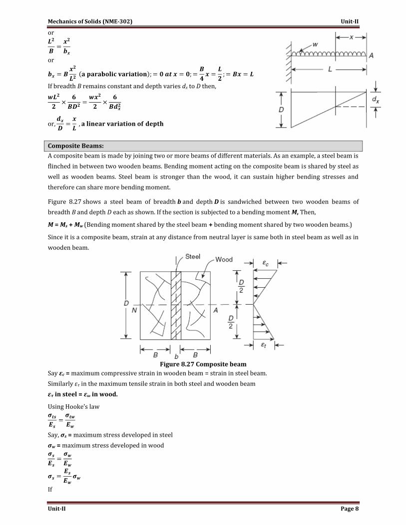
If breadth B remains constant and depth varies dx to D then,

Composite Beams:

A composite beam is made by joining two or more beams of different materials. As an example, a steel beam is

flinched in between two wooden beams. Bending moment acting on the composite beam is shared by steel as

well as wooden beams. Steel beam is stronger than the wood, it can sustain higher bending stresses and

therefore can share more bending moment.

Figure 8.27 shows a steel beam of breadth b and depth D is sandwiched between two wooden beams of

breadth B and depth D each as shown. If the section is subjected to a bending moment M, Then,

M = Ms + Mw (Bending moment shared by the steel beam + bending moment shared by two wooden beams.)

Since it is a composite beam, strain at any distance from neutral layer is same both in steel beam as well as in

wooden beam.

Figure 8.27 Composite beam

Say εc = maximum compressive strain in wooden beam = strain in steel beam.

Similarly ετ in the maximum tensile strain in both steel and wooden beam

ετ in steel = εω in wood.

Using Hooke’s law

Say, σs = maximum stress developed in steel

σw = maximum stress developed in wood

If


Unit-II

σs = mσs (8.6)

So,

Note that these are rectangular section wooden beams

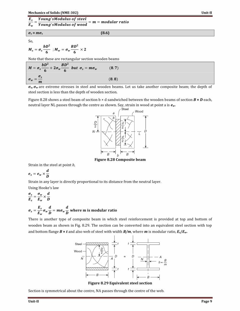
σs, σw are extreme stresses in steel and wooden beams. Let us take another composite beam; the depth of

steel section is less than the depth of wooden section.

Figure 8.28 shows a steel beam of section b × d sandwiched between the wooden beams of section B × D each,

neutral layer NL passes through the centre as shown. Say, strain in wood at point a is ew.

Figure 8.28 Composite beam

Strain in the steel at point b,

Strain in any layer is directly proportional to its distance from the neutral layer.

Using Hooke’s law

There is another type of composite beam in which steel reinforcement is provided at top and bottom of

wooden beam as shown in Fig. 8.29. The section can be converted into an equivalent steel section with top

and bottom flange B × t and also web of steel with width B/m, where m is modular ratio, Es/Ew.

Figure 8.29 Equivalent steel section

Section is symmetrical about the centre, NA passes through the centre of the web.


Unit-II

Section modulus, Z = INA/ymax

Section of the composite beam can also be converted into equivalent wooden section. In that case, steel plates

are converted into equivalent wooden plates of width mB and thickness t remains the same.

If, σs = allowable stress in steel

M = allowable bending moment = σs Z, where Z is section modulus of equivalent steel section.

Reinforced Cement Concrete Beam:

Concrete is a common building material used in the construction of columns and beams which come under

tension and compression due to bending moment acting on these members. While concrete has very useful

strength in compression but it is very weak in tension and so minute cracks may develop in concrete due to

tensile stresses. Therefore, tension side of the beam is reinforced with steel bars. Concrete and steel make a

very good composite material. During setting, concrete contracts and grips the steel reinforcement. Moreover,

the coefficient of thermal expansion of steel and concrete for most common mix is 1:2:4, more or less is the

same. Ratio 1:2:4 stands for 1 part of cement, 2 parts of sand and 4 parts of aggregate by volume.

To develop a theory for RCC structure, following assumptions are made:

1. Concrete is effective only in compression and stress in concrete on the tension side of the beam is zero.

2. Transverse sections which are plane before bending remain plane after bending.

3. Strain in any layer is proportional to its distance from neutral layer.

4. Stress is proportional to strain in concrete also.

5. There is a constant ratio between modulus of elasticity of steel and modulus of elasticity of concrete.

The allowable stresses for concrete and value of Young’s modulus of concrete, Ec depend upon the type of the

concrete mix.

RCC Beams (Rectangular Section)

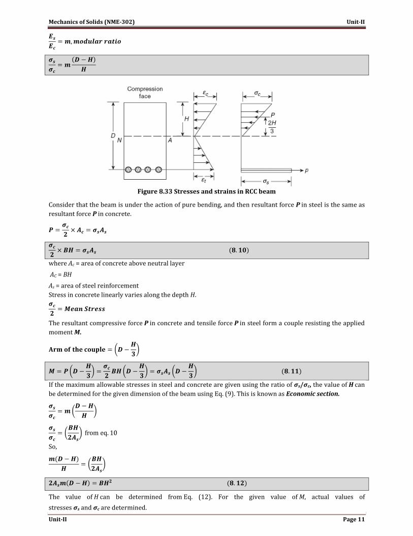
Figure 8.33 shows a rectangular beam of breadth B, depth D (of reinforcement from compression face). Let H

be the distance of neutral axis from the compression face, and maximum stresses developed in steel and

concrete are σs and σc, respectively, as shown in Fig. 8.33.

Strain in any longer is proportional to its distance from neutral layer.

Using Hooke’s Law,

where Es = Young’s modulus of steels

Ec = Young’s modulus of concrete.


Unit-II

Figure 8.33 Stresses and strains in RCC beam

Consider that the beam is under the action of pure bending, and then resultant force P in steel is the same as

resultant force P in concrete.

where Ac = area of concrete above neutral layer

AC = BH

As = area of steel reinforcement

Stress in concrete linearly varies along the depth H.

The resultant compressive force P in concrete and tensile force P in steel form a couple resisting the applied

moment M.

If the maximum allowable stresses in steel and concrete are given using the ratio of σs/σc, the value of H can

be determined for the given dimension of the beam using Eq. (9). This is known as Economic section.

So,

The value of H can be determined from Eq. (12). For the given value of M, actual values of

stresses σs and σc are determined.


Unit-II

Stress Concentration in Bending:

We have learnt about stress concentration due to abrupt change in section due to holes, fillets, grooves etc, in

members subjected to axial loads. In this chapter, we will discuss the effect of fillets, grooves etc., in members

subjected to bending moment on the stress distribution causing high stresses at discontinuity as a fillet and a

groove. If a member is subjected to bending moment M, then stress,

If the flexure member has an abrupt change in geometry then stress change due to this abrupt change in

geometry can be determined by

where K is the stress concentration factor.

Shear Stress Distribution:

Consider a beam of rectangular section with depth D and breadth B. Along the length, consider an elementary

of length dx. On the left side of element the bending moment is M and on the right-hand side of the element

the bending moment is M + dM as shown in the Fig. 9.1(a).

Since there is change in bending moment, there will be a shear force in the section as F = dM/dx , shear force.

Stresses due to M are σc and σt as extreme compressive and tensile stresses, respectively, and stresses due

to M + dM are σc′ and σt′, extreme stresses as shown in Fig. 9.1(b).

Note that σc′ > σc as given in Fig. 9.1(b), similarly σt′ > σt. Due to difference in longitudinal stresses (bending

stresses) on both the sides, there will be difference in resultant. Push (Fc′ − Fc) or pull (on the other side of

neutral layer), which will be balanced by a horizontal force developed on the longitudinal plane of beam Fc′

− Fc = Q = τdxB, where dx and B are the dimensions of longitudinal plane and τ is the shear stress on this

plane.

Figure 9.1 Stresses due to variable bending moment

Any Section (With Variable Breadth):

Now, consider a plane of length dx and breadth b, at a distance y from neutral layer as shown in Fig. 9.2(a).

Beam is subjected to bending moment M on left side and M + dM on right side as shown in the figure.

Consider a layer at a distance y from neutral layer as shown in Fig. 9.2(a). Thickness of layer is dy.

Stress on left side,


Unit-II

Stress as right side,

INA = moment of inertia of section about neutral axis

Figure 9.2 Section with variable width

Forces,

δP = σδa = σbdy

δP′ = σδa = σ′bdy

Summing up all the unbalanced forces on elemental area from y to yc

yc = distance of extreme layer in compression

δF = τbdx where τ is shear stress developed in plane efgh

where

A = area of cross-section above the layer ef (shaded area)

= distance of CG of the area A from neutral layer

or shear stress, τ at distance y from neutral layer

F = shear force; A = area of cross-section above the layer under consideration; = distance of CG of the area

above the layer ; INA = moment of inertia of the section about neutral axis ; b = breadth of the layer

Shear Stress Distribution in a Circular Section of a Beam:

Consider a beam of circular section of diameter D is subjected to a shear force F at the section under

consideration. Neutral layer passes through the centre of the circular section.

Shear force at any layer ab


Unit-II

Consider a layer at a distance y from neutral layer, Fig. 9.6, subtending an angle θ at the centre from neutral

layer.

Substituting the value in Eq. (9.2)

Shear stress distribution is symmetrical on the other side of the neutral layer. Figure 9.6 shows shear stress

distribution along the depth D of the section. Note that the maximum shear stress occurs at neutral axis.

Curves of Principal Stresses in a Beam:

While analyzing the bending stress and shear stress in a beam, it is observed that at the extreme fibres,

bending stress is maximum and shear stress is zero, so the principal stress direction is parallel to the axes of

the beam or the principal plane is perpendicular to the axis at extreme fibres. Similarly at the neutral axes,

bending stress is zero and shear stress is maximum, principal stress inclined at 45° to neutral axis. At any

other layer, there is a combination of normal stress due to bending and shear stress due to transverse shear

force and principal stresses and their directions can be worked out. Then, the curves for principal planes can

be drawn. At any point along the curve, a principal plane is tangential to the curve. There are two sets of

stress curves known as curves of principal stresses as shown in Fig. 9.8.

Two sets of curves of principal stresses/principal planes possess following characteristics:

1. Tangent and normal to these curves give directions of principal stresses and principal planes.

2. Two curves intersect each other at right angles.

3. Curves cross the neutral axes at 45°.

4. Curves are normal to top and bottom surfaces.

5. The intensity of principal stress is maximum when it is parallel to the axes of the beam.

Figure 9.6 Shear stress distribution in a circular section


Unit-II

Figure 9.8 Curves of principal planes

Directional Distribution of Shear Stresses:

A shear stress is always accompanied by a complementary shear stress at right angles. Therefore, the

directions of shear stresses on an element are either both towards the corner or both away from the corner to

produce balancing couples. However, near a free boundary, the shear stress at any section acts in a direction

parallel to the boundary as shown in Figs 9.9(a) and 9.9(b) for an I-section and a circular-section,

respectively. Note that in a circular section, shear stress is parallel to the boundary and at the centre the shear

stress is perpendicular to the boundary, so as to provide complementary shear stress to the shear stress

along the boundary.

In I-section, note that shear stress has to follow the boundary of flange and the web; therefore, the

distribution of shear stress in I-section is as shown in Fig. 9.9(a).

Figure 9.9 Directional distribution of shear stress

Deflection of Beams

Assumption:

The following assumptions are undertaken in order to derive a differential equation of elastic curve for the

loaded beam:

1. Stress is proportional to strain i.e. hooks law applies. Thus, the equation is valid only for beams that are not

stressed beyond the elastic limit.

2. The curvature is always small.

3. Any deflection resulting from the shear deformation of the material or shear stresses is neglected.

Consider a beam AB which is initially straight and horizontal when unloaded. If under the action of loads the

beam deflects to a position A'B' under load or in fact we say that the axis of the beam bends to a shape A'B'. It

is customary to call A'B' the curved axis of the beam as the elastic line or deflection curve.

In the case of a beam bent by transverse loads acting in a plane of symmetry, the bending moment M varies

along the length of the beam and we represent the variation of bending moment in B.M diagram. Futher, it is

assumed that the simple bending theory equation holds good.


Unit-II

If we look at the elastic line or the deflection curve, this is obvious that the curvature at every point is

different; hence the slope is different at different points. To express the deflected shape of the beam in

rectangular co-ordinates let us take two axes x and y, x-axis coincide with the original straight axis of the

beam and the y – axis shows the deflection.

Futher, let us consider an element ds of the deflected beam. At the ends of this element let us construct the

normal which intersect at point O denoting the angle between these two normal be di. But for the deflected

shape of the beam the slope i at any point C is defined,

Further

ds = R di

However

ds = dx (usually for small curvature)

Hence, ds = dx = R di

Substituting the value of i

From the simple bending theory

So the basic differential equation governing the deflection of beam is

This is the differential equation of the elastic line for a beam subjected to bending in the plane of symmetry.

Its solution y = f(x) defines the shape of the elastic line or the deflection curve as it is frequently called.

Relationship between Shear Force, Bending Moment and Deflection:

The relationship among shear force, bending moment and deflection of the beam may be obtained as

Differentiating the equation as derived

Thus

Therefore, the above expression represents the shear force whereas rate of intensity of loading can also be

found out by differentiating the expression for shear force.

Therefore if ‘y’ is the deflection of the loaded beam following relations can be derived.

Methods for Finding the Deflection:


Unit-II

The deflection of the loaded beam can be obtained various methods. The one of the method for finding the

deflection of the beam is the direct integration method, i.e. the method using the differential equation which

we have derived.

Direct Integration Method:

The governing differential equation is defined as

on integrating one get,

Again integrating

Where A and B are constants of integration to be evaluated from the known conditions of slope and

deflections for the particular value of x.

The Area-Moment / Moment-Area Methods:

The area moment method is a semi graphical method of dealing with problems of deflection of beams

subjected to bending. The method is based on a geometrical interpretation of definite integrals. This is

applied to cases where the equation for bending moment to be written is cumbersome and the loading is

relatively simple.

Let us recall the figure, which we referred while deriving the differential equation governing the beams. It

may be noted that dθ is an angle subtended by an arc element ds and M is the bending moment to which this

element is subjected.

We can assume,

ds = dx [since the curvature is small]

hence, R dq = ds

But for small curvature

Hence

The relationship as described in equation (1) can be given a very simple graphical interpretation with

reference to the elastic plane of the beam and its bending moment diagram.

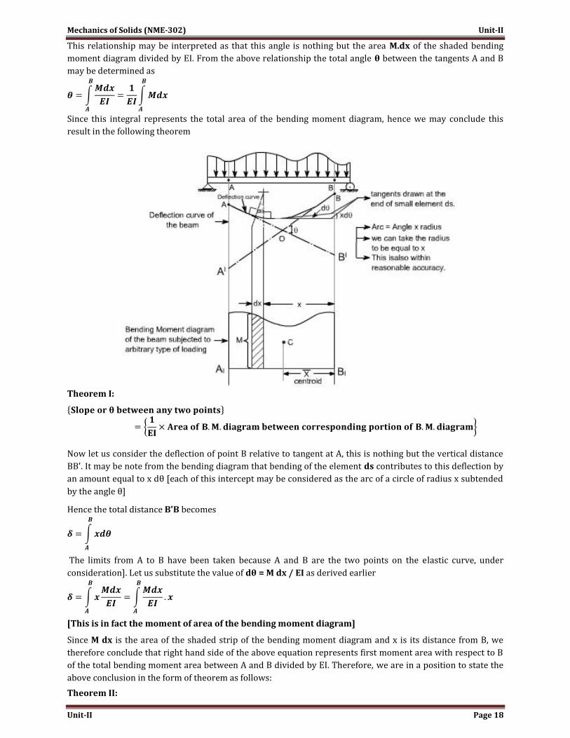
Refer to the figure shown below. Consider AB to be any portion of the elastic line of the loaded beam and

A1B1is its corresponding bending moment diagram.

Let AO = Tangent drawn at A ; BO = Tangent drawn at B

Tangents at A and B intersects at the point O. Futher, AA’ is the deflection of A away from the tangent at B

while the vertical distance B'B is the deflection of point B away from the tangent at A. All these quantities are

further understood to be very small.

Let ds ≈ dx be any element of the elastic line at a distance x from B and an angle between at its tangents be

dq. Then,


Unit-II

This relationship may be interpreted as that this angle is nothing but the area M.dx of the shaded bending

moment diagram divided by EI. From the above relationship the total angle θ between the tangents A and B

may be determined as

Since this integral represents the total area of the bending moment diagram, hence we may conclude this

result in the following theorem

Theorem I:

Now let us consider the deflection of point B relative to tangent at A, this is nothing but the vertical distance

BB'. It may be note from the bending diagram that bending of the element ds contributes to this deflection by

an amount equal to x dθ [each of this intercept may be considered as the arc of a circle of radius x subtended

by the angle θ]

Hence the total distance B'B becomes

The limits from A to B have been taken because A and B are the two points on the elastic curve, under

consideration]. Let us substitute the value of dθ = M dx / EI as derived earlier

[This is in fact the moment of area of the bending moment diagram]

Since M dx is the area of the shaded strip of the bending moment diagram and x is its distance from B, we

therefore conclude that right hand side of the above equation represents first moment area with respect to B

of the total bending moment area between A and B divided by EI. Therefore, we are in a position to state the

above conclusion in the form of theorem as follows:

Theorem II:


Unit-II

Futher, the first moment of area, according to the definition of centroid may be written as , where is

equal to distance of centroid and a is the total area of bending moment

Therefore, the first moment of area may be obtained simply as a product of the total area of the B.M diagram

between the points A and B multiplied by the distance to its centroid C. If there exists an inflection point or

point of contraflexure for the elastic line of the loaded beam between the points A and B, as shown below,

Then, adequate precaution must be exercised in using the above theorem. In such a case B. M diagram gets

divide into two portions +ve and –ve portions with centroids C1and C2. Then to find an angle θ between the

tangents at the points A and B

And similarly for the deflection of B away from the tangent at A becomes

Macaulay's Methods: If the loading conditions change along the span of beam, there is corresponding change in moment equation.

This requires that a separate moment equation be written between each change of load point and that two

integration be made for each such moment equation. Evaluation of the constants introduced by each

integration can become very involved. Fortunately, these complications can be avoided by writing single

moment equation in such a way that it becomes continuous for entire length of the beam in spite of the

discontinuity of loading.

Note: In Macaulay's method some author's take the help of unit function approximation (i.e. Laplace

transform) in order to illustrate this method, however both are essentially the same.

For example consider the beam shown in fig below:

Let us write the general moment equation using the definition M = (∑ M)L, Which means that we consider the

effects of loads lying on the left of an exploratory section. The moment equations for the portions AB, BC and

CD are written as follows:

It may be observed that the equation for MCD will also be valid for both MAB and MBC provided that the terms

(x - 2) and (x - 3)2are neglected for values of x less than 2 m and 3 m, respectively. In other words, the terms

(x - 2) and (x - 3)2 are nonexistent for values of x for which the terms in parentheses are negative.

As an clear indication of these restrictions, one may use a nomenclature in which the usual form of

parentheses is replaced by pointed brackets, namely, ‹ ›. With this change in nomenclature, we obtain a single

moment equation


Unit-II

Which is valid for the entire beam if we postulate that the terms between the pointed brackets do not exists

for negative values; otherwise the term is to be treated like any ordinary expression.

As an example, consider the beam as shown in the fig below. Here the distributed load extends only over the

segment BC. We can create continuity, however, by assuming that the distributed load extends beyond C and

adding an equal upward-distributed load to cancel its effect beyond C, as shown in the adjacent fig below. The

general moment equation, written for the last segment DE in the new nomenclature may be written as:

It may be noted that in this equation effect of load 600 N won't appear since it is just at the last end of the

beam so if we assume the exploratory just at section at just the point of application of 600 N than x = 0 or else

we will here take the X - section beyond 600 N which is invalid.

Procedure to solve the problems:

(i) After writing down the moment equation which is valid for all values of ‘x' i.e. containing pointed brackets,

integrate the moment equation like an ordinary equation.

(ii) While applying the B.C's keep in mind the necessary changes to be made regarding the pointed brackets.

Examples:

1. A concentrated load of 300 N is applied to the simply supported beam as shown in Fig. Determine the

equations of the elastic curve between each change of load point and the maximum deflection in the beam.

Solution: writing the general moment equation for the last portion BC of the loaded beam,

Integrating twice the above eq. to obtain slope and deflection


Unit-II

To evaluate the two constants of integration. Let us apply the following boundary conditions:

1. At point A where x = 0, the value of deflection y = 0. Substituting these values in Eq. (3) we find C2 = 0.keep

in mind that < x -2 >3 is to be neglected for negative values.

2. At the other support where x = 3m, the value of deflection y is also zero. Substituting these values in the

deflection Eq. (3), we obtain

Having determined the constants of integration, let us make use of Eqs. (2) and (3) to rewrite the slope and

deflection equations in the conventional form for the two portions.

Continuing the solution, we assume that the maximum deflection will occur in the segment AB. Its location

may be found by differentiating Eq. (5) with respect to x and setting the derivative to be equal to zero, or,

what amounts to the same thing, setting the slope equation (4) equal to zero and solving for the point of zero

slope. We obtain

50 x2 – 133 = 0 or x = 1.63 m

(It may be kept in mind that if the solution of the equation does not yield a value < 2 m then we have to try the

other equations which are valid for segment BC)

Since this value of x is valid for segment AB, our assumption that the maximum deflection occurs in this

region is correct. Hence, to determine the maximum deflection, we substitute x = 1.63 m in Eq (5), which

yields

The negative value obtained indicates that the deflection y is downward from the x axis. Quite usually only

the magnitude of the deflection, without regard to sign, is desired;

if E = 30 Gpa and I = 1.9 x 106 mm4 = 1.9 x 10 -6 m4

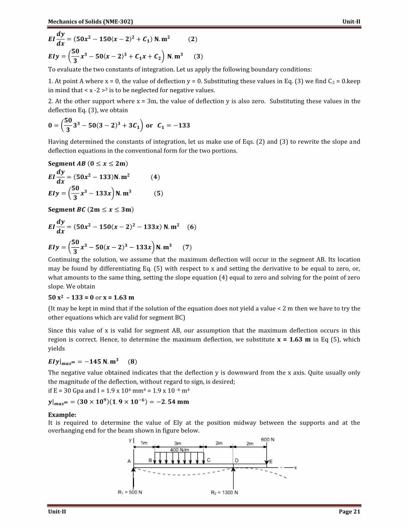
Example: It is required to determine the value of EIy at the position midway between the supports and at the overhanging end for the beam shown in figure below.


Unit-II

Solution: Writing down the moment equation which is valid for the entire span of the beam and applying the

differential equation of the elastic curve, and integrating it twice, we obtain

To determine the value of C2, It may be noted that EIy = 0 at x = 0, which gives C2 = 0.Note that the negative

terms in the pointed brackets are to be ignored Next, let us use the condition that EIy = 0 at the right support

where x = 6m.This gives

Finally, to obtain the mid-span deflection, let us substitute the value of x = 3m in the deflection equation for the segment BC obtained by ignoring negative values of the bracketed terms. We obtain

For the overhanging end where x = 8 m,

Stresses in a Shaft Subjected to Twisting Moment:

A shaft in transmitting power, that is, the torque, is under pure torsion. Due to the torque T, the maximum

shear stress developed on the surface of the shaft is τ = 16T/πd3, where d is the diameter of a solid shaft.

Figure 12.11(a) shows shear stress τ at the surface of the shaft and a complementary shear stress τ at right

angles (i.e., in longitudinal direction). State of stress on a small element on the surface of the shaft is shown

in Figure 12.11(a). Figure 12.11(b) shows complementary shear stress τ at right angles, variation of shear

stress along the radius of the shaft. Figure 12.11(c) shows the enlarged view of the stresses on a small

element. At angle θ = ±45°, principal stresses are developed, p1 = ± τ and p2 = –τ

Figure 12.11(d) shows the development of principal stresses on a small element with direction of principal

stress ± 45° to the axes of the shaft.

So, principal stresses at a point are +τ, –τ, 0.

Principal strains,

Volumetric strain,

This shows that if a shaft is subjected to a pure twisting moment there will not be any change is its

volume.

However, the shafts are subjected to bending moments also due to the forces on elements mounted on shaft

as gears, pulleys and due to reactions from the supports. Therefore, a shaft is subjected simultaneously to a

bending moment M and a twisting moment T at any section shown in Fig. 12.12.


Unit-II

Figure 12.11

Shafts Subjected to T and M:

When a shaft transmits torque T, it is simultaneously subjected to bending moments also due to belt tensions

on a pulley, tooth load on gears and support reactions in bearings. Figure 12.12 shows a shaft subjected to

twisting moment T and a bending moment M. If we take small elements on the surface of the shaft, stresses

acting on the element will be as shown in Figure 12.13.

Figure 12.12 Twisting and bending moments on a shaft

σ = Normal stress due to bending moment M = 32 M/πd3

τ = Shear stress due to twisting moment M = 16 T/πd3

Maximum principal stress at element

The bending moment due to maximum principal stress in shafts is known as equivalent bending

moment, Me.

Figure 12.13 Stresses on a small element

of shaft


Unit-II

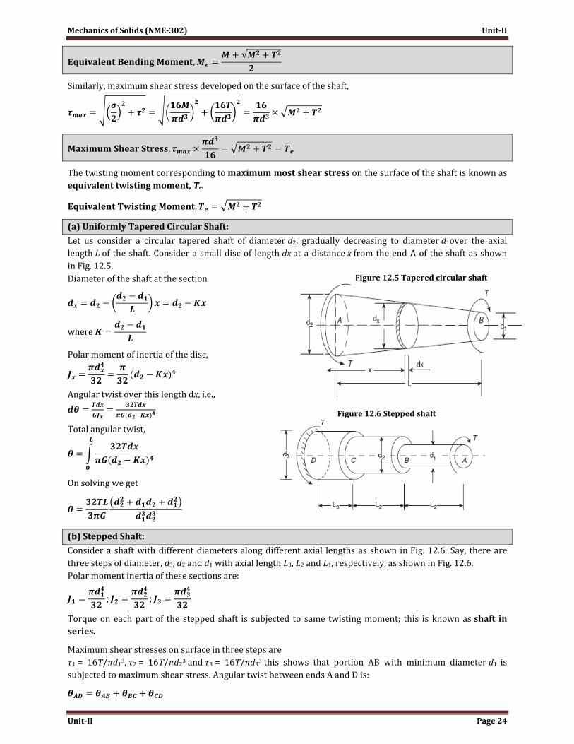
Similarly, maximum shear stress developed on the surface of the shaft,

The twisting moment corresponding to maximum most shear stress on the surface of the shaft is known as

equivalent twisting moment, Te.

(a) Uniformly Tapered Circular Shaft:

Let us consider a circular tapered shaft of diameter d2, gradually decreasing to diameter d1over the axial

length L of the shaft. Consider a small disc of length dx at a distance x from the end A of the shaft as shown

in Fig. 12.5.

Diameter of the shaft at the section

Polar moment of inertia of the disc,

Angular twist over this length dx, i.e.,

Total angular twist,

On solving we get

(b) Stepped Shaft:

Consider a shaft with different diameters along different axial lengths as shown in Fig. 12.6. Say, there are

three steps of diameter, d3, d2 and d1 with axial length L3, L2 and L1, respectively, as shown in Fig. 12.6.

Polar moment inertia of these sections are:

Torque on each part of the stepped shaft is subjected to same twisting moment; this is known as shaft in

series.

Maximum shear stresses on surface in three steps are

τ1 = 16T/πd13, τ2 = 16T/πd2

3 and τ3 = 16T/πd33 this shows that portion AB with minimum diameter d1 is

subjected to maximum shear stress. Angular twist between ends A and D is:

Figure 12.5 Tapered circular shaft

Figure 12.6 Stepped shaft


Unit-II

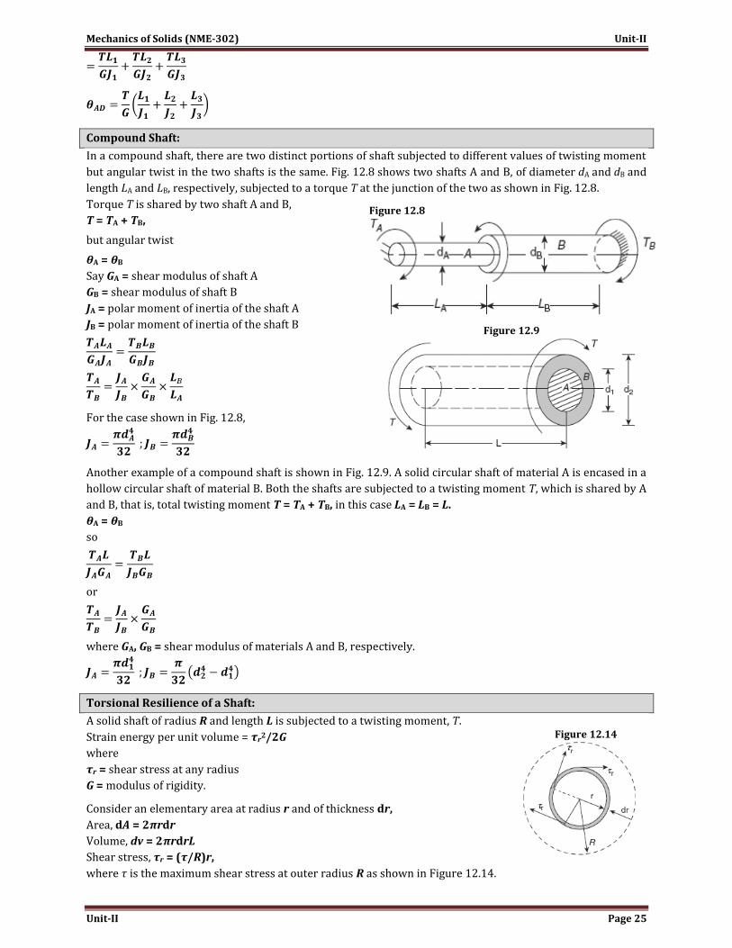
Compound Shaft:

In a compound shaft, there are two distinct portions of shaft subjected to different values of twisting moment

but angular twist in the two shafts is the same. Fig. 12.8 shows two shafts A and B, of diameter dA and dB and

length LA and LB, respectively, subjected to a torque T at the junction of the two as shown in Fig. 12.8.

Torque T is shared by two shaft A and B,

T = TA + TB,

but angular twist

θA = θB

Say GA = shear modulus of shaft A

GB = shear modulus of shaft B

JA = polar moment of inertia of the shaft A

JB = polar moment of inertia of the shaft B

For the case shown in Fig. 12.8,

Another example of a compound shaft is shown in Fig. 12.9. A solid circular shaft of material A is encased in a

hollow circular shaft of material B. Both the shafts are subjected to a twisting moment T, which is shared by A

and B, that is, total twisting moment T = TA + TB, in this case LA = LB = L.

θA = θB

so

or

where GA, GB = shear modulus of materials A and B, respectively.

Torsional Resilience of a Shaft:

A solid shaft of radius R and length L is subjected to a twisting moment, T.

Strain energy per unit volume = τr2/2G

where

τr = shear stress at any radius

G = modulus of rigidity.

Consider an elementary area at radius r and of thickness dr,

Area, dA = 2πrdr

Volume, dv = 2πrdrL

Shear stress, τr = (τ/R)r,

where τ is the maximum shear stress at outer radius R as shown in Figure 12.14.

Figure 12.14

Figure 12.8

Figure 12.9


Unit-II

Strain energy for an elementary volume dv,

Strain energy for the solid shaft,

Note that τ is the maximum shear stress on the surface of the shaft.

Hollow shaft (inner radius R1 and outer radius R2)

τr, at any radius r = (τ/R2)r, R2 is maximum radius.

Strain energy for an elementary volume,

Stress Concentration in Torsional Loading:

Using the torsion formula, we determine the shear stress developed in a shaft of uniform diameter. However,

if the shaft has abrupt change in section such as fillet radius, groove or notch, stress concentration will occur

near the abrupt change in diameter of shaft.

Where,

Ri = radius of smaller diameter at abrupt change.

T = torque.

J = polar moment of inertia for section for smaller diameter.

K = stress concentration factor due to abrupt change.

Magnitude of stress concentration factor K depends upon the ratio of D/d and the ratio of r/d at the fillet.

Similarly, for a grooved shaft the value of K depends on the ratio of D/d and r/d where r is the groove radius.

For shaft with keyways, which are generally used to connect gears, pulleys and flywheels on shaft, ASME

allows 25% reduction in allowable stress using the equation, τ = TR2/T, where R2 is outer radius of the shaft.

mos unit ii

Engineering