ms excel 2007 tutorial

For Any Assistance contact Aditya Chaudhary at [email protected] or visit http://adityamacro.blogspot.in/

MS-Excel 2007 Tutorial

Introduction

Nothing is difficult once you have learned it that applies to excel as well and once you

have learned it, you will be able to do things you never dreamed of! You will be able;

to make calculations more comply than NASA did when they sent the first man to the

moon.

It may sound like big words, but in the case of excel or spreadsheet programs

in general- it is quite true. Spreadsheets can process large amounts of data and give

you the calculation results in no time. And when the calculations are made, you can

have then presented as beautiful tables and graphs.

I know of many who are reluctant to engage with excel because they find it

difficult. Granted, excel is a program that requires some basic skills before embarking

on it. And if you have no feeling for or interest in numbers it can appear meaningless.

With word-processing programs like word you can basically just start typing right

away but with spreadsheets it is a different story.

In return, you can achieve some pretty amazing results when you master excel at

reasonable level. I have made such diverse things as budgets, accounting, production

count, Monthly payouts sheets, break timing maintain in excel and as long as it

involves numbers the only limit is your imagination.

Excel is a program that you never quite finish learning about I have used excel for

many years and have tried most things and I still find it challenging.

Even if you are familiar with all the basic functions, you will find occasion to continue

challenging ourselves and find new things you can squeeze out of the program. And

when the program cannot perform the tasks you require, it also has an entire

programming language, enabling you to make your own small programs inside excel.

I would think excel is the program in the office package which over time has

had the greatest impact on the business sector. Being a number nerd I find it hard to

hide my enthusiasm for excel. I hope that after you finished reading this book, you

will also have discovered how powerful a tool you now have at your disposal.

mailto:[email protected]

http://adityamacro.blogspot.in/


A Small Reader’s Guide

If you have not worked with excel before, I would recommend that you read the

entire book from one end to another. You can subsequently use it as a reference. I

have tried to arrange the book in a logical manner so you can quickly find the chapter

that deals with a problem similar to the one you are trying to solve.

When I ask you to click on something. It is click with left mouse button. A double click

is two fast clicks with left mouse button. If I want you to click the right mouse button,

I call it a right click.

Buttons and menus that you can click are always written in underlined font this

means that when you see underlined text you should be able to find something

similar on the screen that you can click on.

If I want you to type something in you spreadsheet, it will appear like this:

Type=sum (a1:b3)

Now we are ready to start up the program and look at all its wonderful features.

1. First look at excel

In this section we will review the basic structure of excel 2007. You start the

program by clicking the windows start button at the left, then click programs.

In the programs menu you will find a folder called Microsoft office, which is where




excel is located.

i. The screen and its elements

When you start excel, you will automatically start in a new, blank workbook.

Excel basically looks and works the same way it has in the last visions. If you

already know excel, you can use it exactly as you have always done.

Nevertheless, there have been some changes an improvements different

places, and they are not just cosmetic.

ii. Workbooks and spreadsheets

An ordinary excel file is called a workbook and can contain different things.

The most important thing is that it can contain worksheets, but it may also

contain chart sheets and small programs that you can do yourself. The most

important thing is to be aware that an excel file is not necessarily just a

spreadsheet but a workbook that can contain many spreadsheets and

charts.

iii. The ribbon

The ribbon with its tabs and buttons is located at the top. The ribbon is the

most obvious change in excel compared to previous versions, and it

replaces the old menus and toolbars. But the ribbon does not replace only

the menus and toolbars. Many functions which previously required that you

filled out various dialog boxes have become more directly accessible in the

ribbon.

In my case it took some time to get used to the ribbon because I have been

accustomed to the menu bar and toolbars for many years. The ribbon is far




more visual and task oriented and it looks very nice. Whether it is an

improvement is perhaps a matter of tasted. It was difficult for me to get

used to it after so many years with the menu bar and toolbars.

But somehow, I have become quite fond of it. The old toolbar had a

tendency to mess around at the top of the screen, whereas the ribbon stays

in place, so when you need a button, it will be in the same place as last time

you used it.

There are also many exciting new features for formatting and graphics, and

the old shortcut keys also still work.

It is also a great improvement that small tool tips pop up when you point to a button that

has been upgraded. They have nice graphics and more detailed explanations of what the

button does. It is a great help when you want to know the program.

iv. The office button

In the top left corner of the screen you will find the round office button it

corresponds by and large to the old file menu.

If you flick on the office button a menu pops up. This is the menu you must

enter when you want to create a new blank spreadsheet, and when you

need to save it.




Figure4: Clicking on the office button opens this menu

It is also via the office button that you can find excel options, where you can change the

settings for how excel should work.

v. Quick access

This small discrete toolbar quick access, where with a single click you can save, undo, etc., is

located just to the right of the office button. Quick access can be customised so that you

can choose the features that suit you best. You do this by right clicking on a button and

choosing customize quick access toolbar. Alternatively you can click the small arrow to the

right of the toolbar, which enables you to quickly select and deselect various features.

vi. The workspace

The workspace is located underneath the ribbon, and this is where you have your

spreadsheet. The spreadsheet is a huge table with columns and rows. The columns are

named with letters in the column headings and the rows are labelled with row numbers in

the row headings. By clicking on a column heading. You can select the cells in the whole

column, and the same is true if you click on a row heading.

The corner is located in the top left corner of the worksheet. By clicking on the corner you

can select all the cells in the entire worksheet.

The cells are the basic elements of the worksheet; this is where we type in our data and

formulas. Wherever a row and a column meet, we have cell. Each cell in the worksheet has

a unique name. For example, the cell located where column C and row 4 meet is called C4.

A cell can contain numbers, words and formulas.

Formulas are a kind of commands that you type into a cell, which make the cell display the

result of a calculation. You do not have to worry about that yet, I promise we will return we

will return to it in more detail.

2. Calculations

The primary objective of excel is to count, and there program is actually quite good at

it.

To make a calculation you must write a formula. The formula should be written into

the cell showing the result. A formula is a structured piece of text that tells excel what it has

to calculate. It is not that hard to learn in small steps, so let us write a simple little formula

to calculate the result of 2+3.




I. Formulas

In excel one always starts a formula by typing an equal sign=. It is a sign that tells

excel that what is in the cell is a formula and not a text or a number. When you are finish

typing the formula, excel will display the result in the cell instead of the formula you have

written.

1. Place the cursor in a random cell and type=2+3

2. Press the ENTER key on the keyboard.

It should now read “5” in the cell in which you wrote the formula. Move the cursor to the

cell, and note that the formula bar still reads “=2+3”, like shown above.

II. Operators

You can use the four methods of calculation (Plus +, minus -, multiply *, and divide /)

in this way. You can also use parentheses if necessary. For example, 2+3*4 is note the same

as (2+3)*4. In this respect excel follows the general calculation rules.

Potency is calculated by using the sign “^”, written by holding down SHIFT on your

keyboard and pressing the key between Z and ENTER. For example, 2^3. It means 2*2*2=8.

So far, you are probably not all that impressed with excel’s calculation capacity.

Actually, we could make the above calculation much easier by using a simple pocket

calculator, and it is only to show what a basic formula is.

III. Formulas with references

To make everything right, we must take advantage of references in our formulas.

References are made to values in other cells. Delete everything you have written in your

spreadsheet so far, and dot the following;

1. In cell B2, type the number 2.

2. In cell B3, type the number 3.

Now it should look like below.




Then do the following

3. Start by typing an=sign into cell B4 to show that you are about to write a formula. Do not type anything

else, and do not press the enter key.

4. Take your mouse, point to cell B2 and click once with left mouse button. Now the formula bar should

show “=B2”.

5. Press the + key on the keyboard. You are hopefully not surprised the it says “=B2+”

6. Take your mouse again, point to cell B3, and click once with the left mouse button. Now it says “=B2+B3”

in the formula bar.

7. Press the enter key on the keyboard.

If the computer did not break down it is now possible to create a formula that adds the values in cell B2 and B3 and

displays the result 5 in cell B4. You should actually be able to write exactly the same formula in a different cell in the

spreadsheet, so let us try it.

8. Choose an empty cell and type the following (without using the mouse):=B2+B3

9. And press enter.

The result is of course the same, but now you have seen that you can freely choose between creating cell references

by clicking with mouse or typing then in directly. Each method has its advantages. When you click the mouse you do

not risk making typos but typing is often faster.

The great thing about the formulas is that they keep working. If you change the numbers in cells B2 and B3 the

results in the cells with formulas also change so go ahead and try writing some other number in cell B2 and B3.

In the next section, we will try using some of excel’s built-in “functions” in our formulas.

IV. References to other spreadsheets

You are not limited to refer to cells in the same spreadsheet. In excel you can have multiple

spreadsheets in the same excel file, and they are, as mentioned previously, organised in the

sheet tabs at the bottom of the screen.

If you refer to a cell in another worksheet, the reference must contain both a sheet

reference and a cell reference.

If you type a formula in sheet1, that user the value from cell B2 in ark2, the reference must

be “sheet2!B2” not just “B2”, which would be a reference to the sheet you are currently

working in.

You can also refer to cells in other spreadsheets files; we will return to that eventually.




V. Functions

When I talk about “functions”, I mean functions in formulas. These are not functions such as

“print” or “Save”, but calculation functions. In the previous section you learned how to

write simple formulas, where you could calculate with a few number. Functions enable you

to add thousands of numbers together in an instant, calculate averages, and make

probability calculations and many other things.

Functions are used in the formulas, and you can use several functions in the same formula.

If we want to be really advanced we can even use functions within other cautions but we

will not got that far yet.

All functions in excel are written in a certain way, which can be summed up in this manner.

Functions Name (Arguments)

All functions have a function name. For example, the function that adds together number is

called “SUM”, and the function that calculates averages is called “Average”. The function

name is followed by one or more “Arguments”, which are the numbers or cell references

that feature must use in the calculation. If there is more than one argument in a function,

they are separated by a semicolon”;” It looks like this

Function name (argument 1; argument2; argument3)

Let us explore the most common functions, SUM and AVERAGE.

The SUM Function:

Now you will learn how to add together many numbers in an instant, but let us start with

something simple.

1. Type the number 2 in cell B2

2. Type thee number 3 in cell B3

3. Type the number 4 in cell B4

Now we will type a formula into cell b% to add together the numbers in cells B2, B3 and B4.

4. In cell B5, write enter=SUM (B2:B3:B4). You will see that excel colours the cell

references and frames the corresponding cells in the same colour. It is helpful later

when you work with more complicated formulas.

5. Press the ENTER key.




Cell B5 should now show the result 9. If it did not work, check that you remembered to

write and equal sign at the beginning of the formula.

You have written a formula with a SUM function with three arguments: the three cell

references are separated by semicolons. Suppose you have to add together 1000 figures

using cell references, that formula would be very long. It is, therefore, possible to use a

“Region reference” as an argument.

A region reference consists of two cell references separated by a Colon “:”. Excel will add

together the two cells AND all the cells between them.

1. Select cell B5 and press the F2 key on the keyboard.

2. Rewrite the formula so it reads=SSUM (B2:B4) and press the ENTER key. Remember

this time there should be a colon “:” in the function, not a semicolon “;”.

The result is the same as last time, but you have now given one argument instead of three

arguments, namely the region reference “B2:B4”. Since cell B3 is between B2 and B4, it is

part of the region that defines the calculation.

If the list had has 1000 numbers that were to be added together instead of three, the

formula would simply be called =SUM (B2:B1001). So now you know how to add together

the 1000 numbers in an instant.

By the way, the SUM function does not care if there are empty cells in the region specified.

Now you have probably made an effort to write the formulas, just like I asked you to. I can

tell you, that when you write formulas excel is completely indifferent to whether you use

uppercase or lowercase. So now you do not need to think about that anymore.




The AVERAGE Function:

The AVERAGE function is used exactly like the SUM function, but it calculates the average of

the arguments instead. The nice thing about the AVERAGE function is that if there are

empty cells in your arguments the AVERAGE function will ignore them. Remember in this

context that an empty cell is not the same as a cell where there is a 0 value.

Now we will write formula with an AVERAGE function, similar to the SUM function we just

had. But this time we will provide the region reference using the mouse in order to get a

little practice.

1. Activate cell B6 and type=AVERAGE(

2. Using the mouse, point to cell B2, press the left mouse button and hold it down.

3. Move the mouse down in order to select cell B2 B3 and B4, then release the left

mouse button. Now it should say= AVERAGE(B2:B4

4. Close the brackets “)” and press ENTER.

Cell B6 should now show the result 3.




Now macro has completed recording. There is nothing further to do before we play it.




So far we have covered many topics above. Which includes some of below or some are new

to practice yourself.

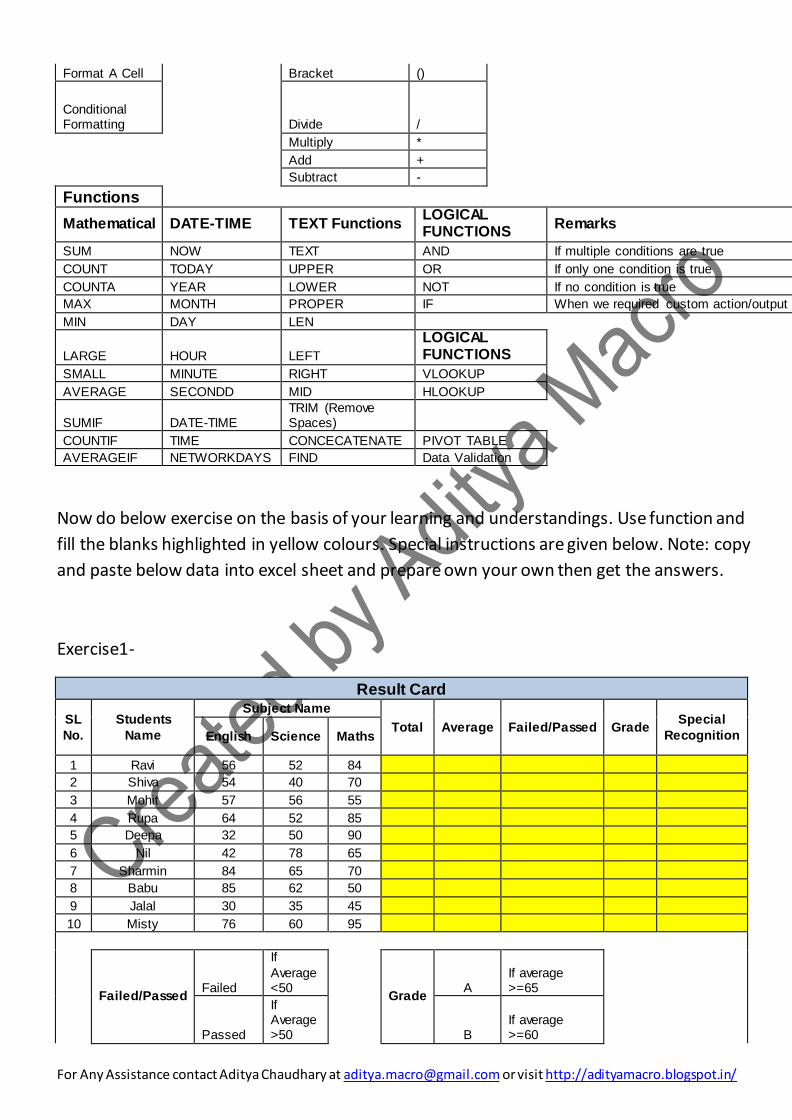
Formatting

Action Operators




Format A Cell

Bracket ()

Conditional Formatting

Divide /

Multiply *

Add +

Subtract -

Functions

Mathematical DATE-TIME TEXT Functions LOGICAL FUNCTIONS

Remarks

SUM NOW TEXT AND If multiple conditions are true

COUNT TODAY UPPER OR If only one condition is true

COUNTA YEAR LOWER NOT If no condition is true

MAX MONTH PROPER IF When we required custom action/output by our logic

MIN DAY LEN

LARGE HOUR LEFT

LOGICAL FUNCTIONS

SMALL MINUTE RIGHT VLOOKUP AVERAGE SECONDD MID HLOOKUP

SUMIF DATE-TIME TRIM (Remove Spaces)

COUNTIF TIME CONCECATENATE PIVOT TABLE AVERAGEIF NETWORKDAYS FIND Data Validation

Now do below exercise on the basis of your learning and understandings. Use function and

fill the blanks highlighted in yellow colours. Special instructions are given below. Note: copy

and paste below data into excel sheet and prepare own your own then get the answers.

Exercise1-

Result Card

SL

No.

Students

Name

Subject Name

Total Average Failed/Passed Grade Special

Recognition English Science Maths

1 Ravi 56 52 84

2 Shiva 54 40 70

3 Mohit 57 56 55

4 Rupa 64 52 85

5 Deepa 32 50 90

6 Nil 42 78 65

7 Sharmin 84 65 70

8 Babu 85 62 50

9 Jalal 30 35 45

10 Misty 76 60 95

Failed/Passed

Failed

If

Average <50

Grade

A If average >=65

Passed

If Average >50

B If average >=60




C If average >=55

Special Recognition Excellent

If Got >70 in

all subjects D If average <55

Exercise2-Use text functions and gets last and first name and Email id as per instruction.

Full Name Last Name

First Name

Email ID

Sok Sibal

Sao Virak

Seng Sabath

Chen Chameroun

get the last name from the full name

get the first name from the full name

get emailid for each person in the form [email protected]

Exercise3-

Bonus Min

Amount Max

Amount

12% 100000 200000

Sales Man Sales Bonus

A 87925

B 100000

C 299555

D 92500

E 122680

F 241041

Sales should be Min & Max to get bonus 12%




Exercise4-

Name Score Rating

Ajay 78 A

Amit 76 A

Vinay 85 A

Hari 45 C

Yatin 67 B

Sunita 43 C

Suraj 47 C

Sakshi 59 C

How may A ratins are there?

How many have got above 70?

What is the average score?

What is the Highest score?

What is the lowest score?

What is the total score B rating?

Exercise5-

Emp Code

Name Region

E001 Bob Delhi

E002 Chriss Bombay

E003 Kennedyy Delhi

E004 Bency Delhi

Emp Code

Region

E004

E003

E001

Exercise6-

City Country ISO

Code Average

Emp

Paris France FR 13

New york USA US 14

London England GB 10

Warsaw Poland PL 8

Oxford England GB 9

Washington USA US 116

Miami USA US 24

Moscow Russia RU 6

Sum of average temp for USA




Count the no of countires where average temp <USA

avg temp

Exercise7-

Salesperson Items

Bought Items Sold

Expenses Income Comission

Dan 3 6 30 60

Maria 3 4 30 40

Izik 8 7 80 70

Brenda 6 4 60 40

Lucy 5 5 50 50

Nathan 3 9 30 90

Brenda 8 6 93 60

Heather 8 4 80 40

Dan 3 4 30 40

Bruce 7 6 70 60

Bring comission of 12% of income if item soldd is more than 5

Get the sum of range I2:I5 and J2:J5

Get the average of the same ranges

Name of sales person Dan Brenda Bruce Izik

Items Sold

Total sold items above 4

Change the font colour of duplicate cell values under the heading income

Highlight the rows where items sold>5

Highlight the highest & lowest expenditure



ms excel 2007 tutorial

Education