ms2001 notes - wordpress.com
TRANSCRIPT
MS2001
Differential Calculus
COURSE NOTES
Stephen Wills
Department of Mathematics
University College Cork
2005/06

Contents
1 Inequalities 3Definitions and axioms . . . . . . . . . . . . . . . . . . . . . . . . . . . . . . 3Sketching functions; the quadratic . . . . . . . . . . . . . . . . . . . . . . . 5Inequalities involving rational functions . . . . . . . . . . . . . . . . . . . . 10The modulus function; obtaining bounds . . . . . . . . . . . . . . . . . . . . 13
2 Limits and Continuity 18The intuitive idea of limits . . . . . . . . . . . . . . . . . . . . . . . . . . . 18The definition of a limit; basic techniques . . . . . . . . . . . . . . . . . . . 20Coping with infinity . . . . . . . . . . . . . . . . . . . . . . . . . . . . . . . 27Continuous functions . . . . . . . . . . . . . . . . . . . . . . . . . . . . . . . 29Continuity on intervals . . . . . . . . . . . . . . . . . . . . . . . . . . . . . . 32
3 Differentiation 35The idea and definition of derivatives . . . . . . . . . . . . . . . . . . . . . . 35The Mean Value Theorem and consequences . . . . . . . . . . . . . . . . . . 42Implicit differentiation . . . . . . . . . . . . . . . . . . . . . . . . . . . . . . 46
4 Curve Sketching and MinMax Problems 49Maxima and minima . . . . . . . . . . . . . . . . . . . . . . . . . . . . . . . 49The second derivative test . . . . . . . . . . . . . . . . . . . . . . . . . . . . 50Applied maximum and minimum problems . . . . . . . . . . . . . . . . . . 54
A number of the examples covered in these notes have appeared on exam papers.This is indicated by expressions such as Example 1.14 (S03 1(a)) which indicatesthat Example 1.14 was question 1(a) from the Summer paper of 2003. SimilarlyExample 1.18 (A02 1(a)) was question 1(a) from the Autumn paper of 2002.

Prologue I: Functions and Fractions
These notes are designed to accompany the course MS2001 Differential Calculus,which provides a more detailed introduction than MS1001 to an area of mathematicsthat was developed to deal with problems in the physical sciences and now has manyapplications in this field and beyond.
In this course we deal with functions of one real variable, that is functions such asx7 − 4x4 + 8x3 − 12x2, 2 sin 3t + t log t or etan x, where the argument is a real number
x, or t, or. . . Complex numbers such as 2+3i (where i =√−1) do not feature in this
course.Such functions will in general be denoted by lower case letters such as f , g or h, or
f(x), g(t) or h(x) if we wish to stress the argument. Note that it is not always possibleto evaluate a function for all possible values of its input variable. For example log xis only defined whenever x > 0, and tan x is only defined for x 6= ±π
2 ,±3π2 , . . . That
is, they are only defined on a subset of the set of all real numbers (which is denotedby the letter R). If we write f : I → R then we mean that f is a function defined onthe subset of I of R, and taking values in the set R of all real numbers. That is, f(x)is a real number that can be evaluated/makes sense whenever we choose any value xfrom the set I.
In a certain sense the main mathematical challenge posed (and solved) by thiscourse arises from the fact that division by 0 is not allowed. In particular expressionssuch as 3
0 or −70 are meaningless, and should not appear in your work. If we divide
one function by another then we must take note of when the denominator is zero.For example consider the function
f(x) =x
sinx.
This is not defined whenever sin x = 0, that is when x = 0,±π,±2π, . . . Howeverconsider what happens as x gets closer and closer to 0:
x = 0.5 0.2 0.1 0.01 · · ·f(x) ≈ 1.04291482 1.00669791 1.00166861 1.00001667 · · ·
The value of f(x) gets closer and closer to 1. However it is still incorrect to writef(0) = 0
sin 0 = 00 = 1, since 0
0 is undefined. But it is precisely the limiting behaviour
of fractions of this sort where both top and bottom approach 0 that we would like tounderstand and deal with rigorously.
On a related note, given two functions g and h the equation
g(x)
h(x)= 0
has a solution when g(x) = 0. The value of h(x) (unless it is also 0) is immaterial.If the above equation holds there is certainly no reason to conclude that g(x) = h(x)
— if this latter equation is true (and both are nonzero) then g(x)h(x) = 1.
1

Prologue II: Notation for Logic
A proposition in logic is a statement that is either true or false. For example
p1: x + y = y + x for all real numbers x and y. (TRUE)
p2: There are 10 month in the year. (FALSE)
Often the proposition may depend on a variable, for example
p3: It is August.
p4: x2 − 4x + 3 = 0.
p3 is only true for 31 days each year, but never during the first semester in UCC. Forp4 note that x2−4x+3 = (x−1)(x−3), and so p4 is true if x = 1 or x = 3, otherwiseit is false.
Given propositions p and q, we write p ⇒ q (read “p implies q”) if q is truewhenever p is true. For example, if we set
p5: Next month is September,
p6: x = 1,
then p3 ⇒ p5, since if it is now August then next month it will be September — thislogical deduction is valid no matter what month it currently is. Similarly p6 ⇒ p4,since if x = 1 then 12 − 4 × 1 + 3 = 0. Note also that if p4 is false, i.e. x is differentfrom 1 or 3, then p6 must be false.
For our examples we also have p5 ⇒ p3, which can be written p3 ⇐ p5. So ifp3 is true then p5 is true; conversely if p5 is true then p3 is also true. Such pairs ofpropositions are called equivalent, which is written p3 ⇔ p5 (read “p3 (is true) if andonly if p5 (is true)”).
However, if p4 is true then either x = 1 or x = 3. If x = 3 then p6 is not true, i.e.p4 6⇒ p6 (“p4 does not imply p6”). Thus these propositions are not equivalent. Allwe can say is that p6 is a sufficient condition for p4, or p4 is a necessary condition forp6.
Mathematical proofs start with clearly stated assumptions and then proceed viaa sequence of propositions, proving that each implies the next, until we end up withthe desired conclusion. That is, our statements are usually linked by ⇒.
2
INEQUALITIES
1 Inequalities
Definitions and axioms
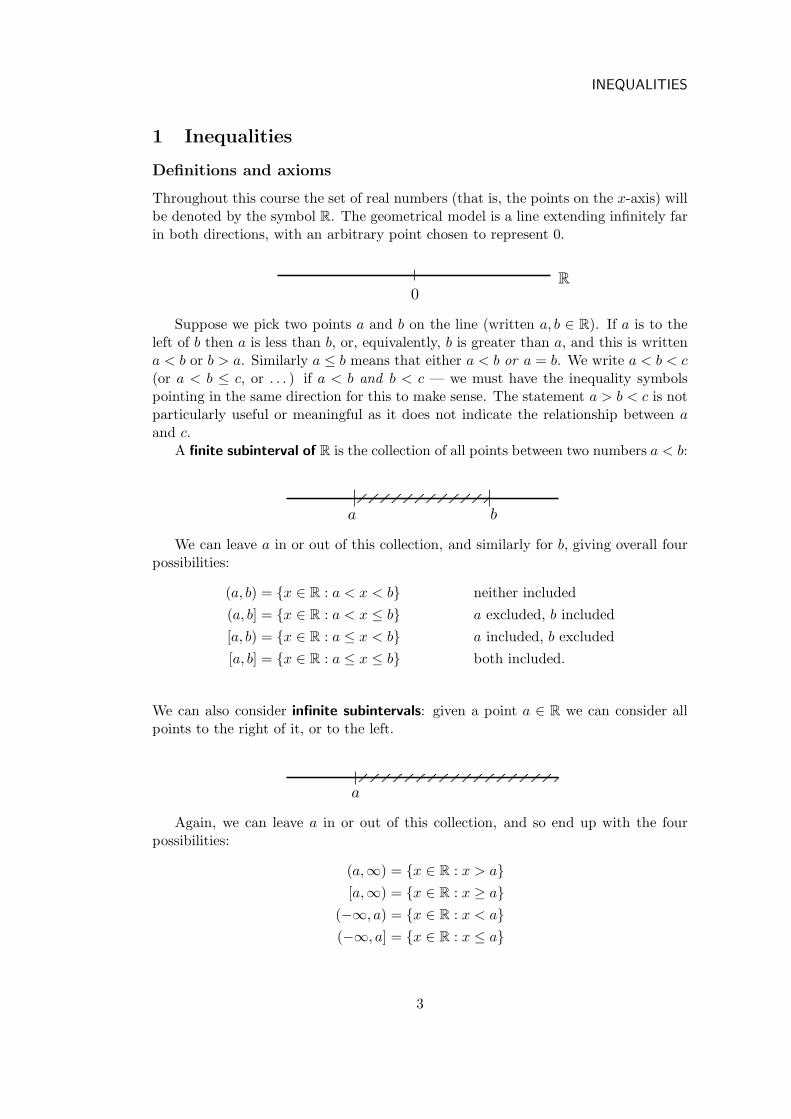
Throughout this course the set of real numbers (that is, the points on the x-axis) willbe denoted by the symbol R. The geometrical model is a line extending infinitely farin both directions, with an arbitrary point chosen to represent 0.
��
0R
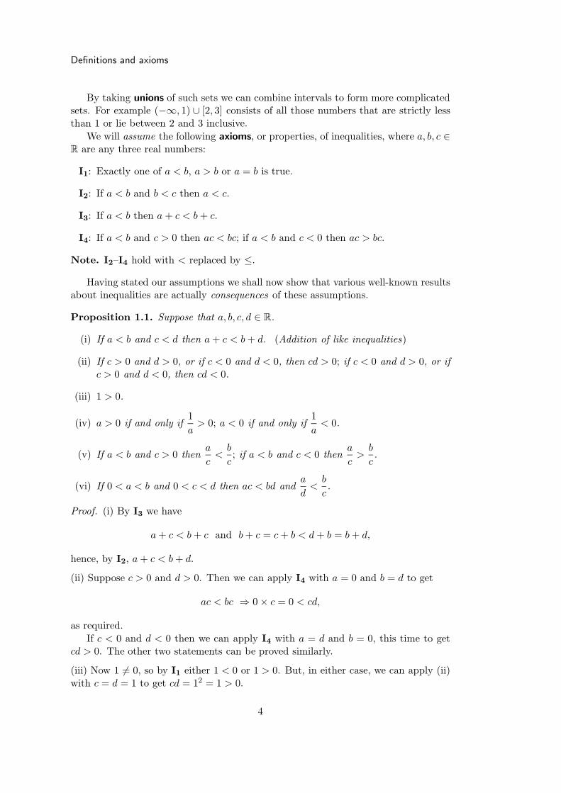
Suppose we pick two points a and b on the line (written a, b ∈ R). If a is to theleft of b then a is less than b, or, equivalently, b is greater than a, and this is writtena < b or b > a. Similarly a ≤ b means that either a < b or a = b. We write a < b < c(or a < b ≤ c, or . . . ) if a < b and b < c — we must have the inequality symbolspointing in the same direction for this to make sense. The statement a > b < c is notparticularly useful or meaningful as it does not indicate the relationship between aand c.
A finite subinterval of R is the collection of all points between two numbers a < b:
����������������
����
a b
We can leave a in or out of this collection, and similarly for b, giving overall fourpossibilities:
(a, b) = {x ∈ R : a < x < b} neither included
(a, b] = {x ∈ R : a < x ≤ b} a excluded, b included
[a, b) = {x ∈ R : a ≤ x < b} a included, b excluded
[a, b] = {x ∈ R : a ≤ x ≤ b} both included.
We can also consider infinite subintervals: given a point a ∈ R we can consider allpoints to the right of it, or to the left.
����������������������a
Again, we can leave a in or out of this collection, and so end up with the fourpossibilities:
(a,∞) = {x ∈ R : x > a}[a,∞) = {x ∈ R : x ≥ a}
(−∞, a) = {x ∈ R : x < a}(−∞, a] = {x ∈ R : x ≤ a}
3
Definitions and axioms
By taking unions of such sets we can combine intervals to form more complicatedsets. For example (−∞, 1) ∪ [2, 3] consists of all those numbers that are strictly lessthan 1 or lie between 2 and 3 inclusive.
We will assume the following axioms, or properties, of inequalities, where a, b, c ∈R are any three real numbers:
I1: Exactly one of a < b, a > b or a = b is true.
I2: If a < b and b < c then a < c.
I3: If a < b then a + c < b + c.
I4: If a < b and c > 0 then ac < bc; if a < b and c < 0 then ac > bc.
Note. I2–I4 hold with < replaced by ≤.
Having stated our assumptions we shall now show that various well-known resultsabout inequalities are actually consequences of these assumptions.
Proposition 1.1. Suppose that a, b, c, d ∈ R.
(i) If a < b and c < d then a + c < b + d. (Addition of like inequalities)
(ii) If c > 0 and d > 0, or if c < 0 and d < 0, then cd > 0; if c < 0 and d > 0, or if
c > 0 and d < 0, then cd < 0.
(iii) 1 > 0.
(iv) a > 0 if and only if1
a> 0; a < 0 if and only if
1
a< 0.
(v) If a < b and c > 0 thena
c<
b
c; if a < b and c < 0 then
a
c>
b
c.
(vi) If 0 < a < b and 0 < c < d then ac < bd anda
d<
b
c.
Proof. (i) By I3 we have
a + c < b + c and b + c = c + b < d + b = b + d,
hence, by I2, a + c < b + d.
(ii) Suppose c > 0 and d > 0. Then we can apply I4 with a = 0 and b = d to get
ac < bc ⇒ 0 × c = 0 < cd,
as required.
If c < 0 and d < 0 then we can apply I4 with a = d and b = 0, this time to getcd > 0. The other two statements can be proved similarly.
(iii) Now 1 6= 0, so by I1 either 1 < 0 or 1 > 0. But, in either case, we can apply (ii)with c = d = 1 to get cd = 12 = 1 > 0.
4
INEQUALITIES
(iv) Suppose a > 0. Again, since 1a 6= 0, we must have 1
a < 0 or 1a > 0. If 1
a < 0,then by (ii) (with c = a and d = 1
a this time) we would have 0 > cd = a × 1a = 1,
contradicting (iii). Hence we must have 1a > 0.
We have shown that if a > 0 then 1a > 0 — and this is true for any positive
number. If, on the other hand we are given a and told 1a > 0, then we now know that
11/a = a > 0. These two implications together give
a > 0 ⇔ 1a > 0.
That a < 0 is equivalent to 1a < 0 can be proved in the same way.
(v) This is immediate from I4 and (iv), since if c > 0 then 1c > 0, and if c < 0 then
1c < 0.
(vi) We have a < b and c > 0, and so ac < bc by I4. Also, c < d and b > 0, and sobc < bd by I4 as well. Thus, by I2,
ac < bd
as required. Finally, cd > 0 by (ii), so by (v)
ac
cd<
bd
cd⇒ a
d<
b
c.
Of particular importance to us are (ii), (iv) and (v). Indeed, it follows that ifwe take any n nonzero numbers a1, a2, . . . , an, and choose any number m satisfying1 ≤ m < n, and then calculate
a1 × a2 × · · · × am
am+1 × · · · × an
then the result will be positive if an even number of the original n numbers ai arenegative, otherwise it will be negative.
Sketching functions; the quadratic
Definition 1.2. A function f : R → R is even if f(−x) = f(x) for all x ∈ R. It isodd if f(−x) = −f(x) for all x ∈ R.
Thus a function is even if it is invariant under reflections in the y-axis, and oddif it is invariant under rotations through π about the origin.
Definition 1.3. Let I ⊂ R be an interval. A function g : I → R is increasing on I ifg(x) ≤ g(y) whenever x, y ∈ I such that x ≤ y. It is strictly increasing if g(x) < g(y)whenever x, y ∈ I such that x < y. What it means for g to be (strictly) decreasing
is defined similarly.
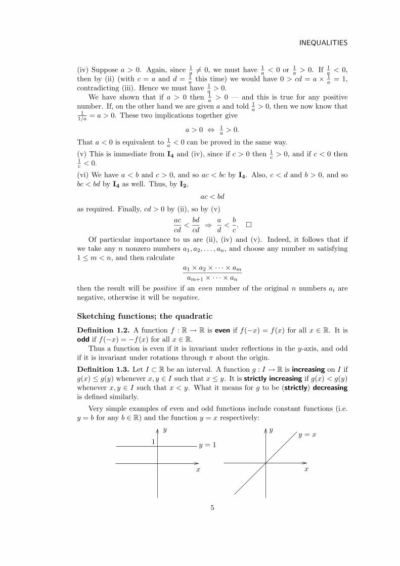
Very simple examples of even and odd functions include constant functions (i.e.y = b for any b ∈ R) and the function y = x respectively:�
�������
��������
����������������������������������
�������
�������
������������������������������������������
������������������������������������������
����������������
yy
xx
y = x
y = 11
5

Sketching functions; the quadratic
Note that the function y = x is strictly increasing on the whole line R, and the con-stant function is both increasing and decreasing on R, but neither strictly increasingnor strictly decreasing.
Other important examples include y = cos x, which is even, and y = sin x whichis odd. Note that y = sinx is (strictly) increasing on the interval [−π
2 , π2 ], decreasing
on [π2 , 3π2 ], and so on.
y = sin xy = cosx
ππ/2
−3π/2
−π
The behaviour of constant functions and y = x generalises to higher powers of n,as can be proved using our consequences of inequalities:
Proposition 1.4. For each positive integer n ≥ 1 let fn : R → R be the function
fn(x) = xn. Then fn is even if n is even, and odd if n is odd. Moreover each fn is
strictly increasing on the half-line [0,∞).
Proof. To see the first part about even or oddness of fn, we can write
fn(−x) = (−x)n = (−1 × x)n = (−1)n × xn =
{xn if n is even,
−xn if n is odd.
For the other part, choose any n ≥ 1. Then note that for any a, b ∈ [0,∞) we have
an − bn = (a − b)(an−1 + an−2b + an−3b2 + · · · + abn−2 + bn−1).
In particular for n = 2 and n = 3 we have
a2 − b2 = (a − b)(a + b) and a3 − b3 = (a − b)(a2 + ab + b2).
But we have chosen a, b ≥ 0, hence any number of the form an−kbk−1 is nonnegativeby part (ii) of Proposition 1.1. Thus, by part (i) of Proposition 1.1,
an−1 + an−2b + an−3b2 + · · · + abn−2 + bn−1 ≥ 0.
Now if a > b ≥ 0 then in particular a > 0, hence an−1 > 0, and it follows that theabove inequality is in fact a strict one. Thus an − bn is the product of two positivenumbers (since a − b > 0), hence positive by part (ii) of Proposition 1.1. That is,
a > b ⇒ an − bn > 0 ⇒ an > bn (by I3)
and so fn is strictly increasing.
6
INEQUALITIES
In fact the above proof shows a little more, since if we have any a, b ∈ [0,∞) thatsatisfy an > bn, then at least one of these two numbers must be nonzero, and hencepositive, and so
an−1 + an−2b + an−3b2 + · · · + abn−2 + bn−1 > 0
again, from which it follows that
a − b =an − bn
an−1 + an−2b + an−3b2 + · · · + abn−2 + bn−1> 0
by part (v) of Proposition 1.1. Hence we have in fact shown the following:
Corollary 1.5. For any integer n ≥ 1 and any a, b ∈ [0,∞) we have
a < b ⇔ an < bn.
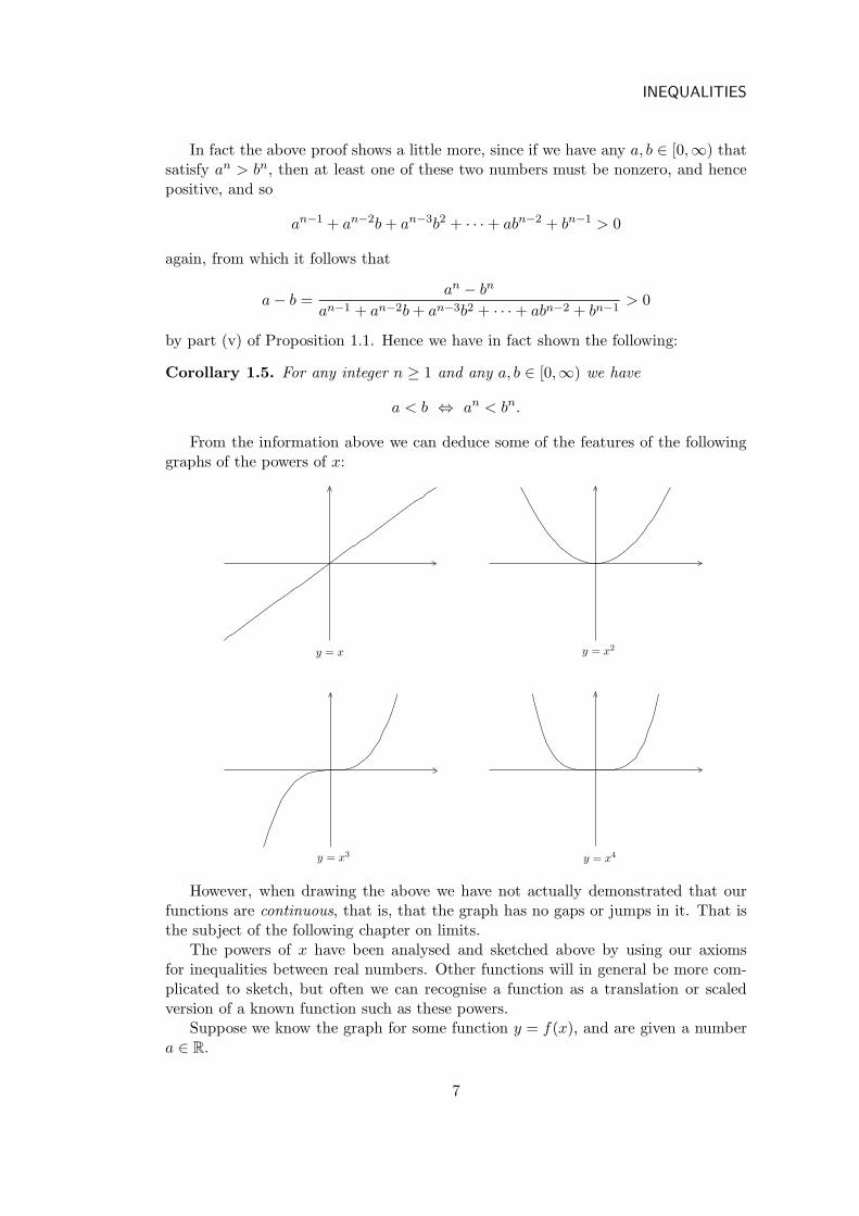
From the information above we can deduce some of the features of the followinggraphs of the powers of x:
y = x y = x2
y = x3 y = x4
However, when drawing the above we have not actually demonstrated that ourfunctions are continuous, that is, that the graph has no gaps or jumps in it. That isthe subject of the following chapter on limits.
The powers of x have been analysed and sketched above by using our axiomsfor inequalities between real numbers. Other functions will in general be more com-plicated to sketch, but often we can recognise a function as a translation or scaledversion of a known function such as these powers.
Suppose we know the graph for some function y = f(x), and are given a numbera ∈ R.
7

Sketching functions; the quadratic
(i) The graph for f(x− a) is got by translating the original a units horizontally tothe right.
(ii) The graph for f(ax) is got by stretching the original horizontally by a scalefactor of 1
a — if a < 0 this involves a reflection in the y-axis and scaling by1−a > 0.
(iii) The graph for f(x) + a is obtained by translating the original vertically by aunits.
(iv) The graph for af(x) is obtained by stretching the original vertically by a scalefactor of a — again if a < 0 this involves a reflection in the x-axis and thenscaling by −a > 0.
Example 1.6. Consider the function y = sin x. The functions sin(x − π2 ), sin 2x,
sinx + 1 and −3 sin x are obtained by applying the relevant rules from above to give:
sinx sin(x − π
2)
sinx + 1
sin 2x
−3 sinx
For example sin(0− π2 ) = sin(−π
2 ) = −1, the value of sin x taken π2 units to the left,
sin(π2 − π
2 ) = sin(0) = 0, etc. Similarly sin(2× π4 ) = sin π
2 = 1, sin(2× π2 ) = sin π = 0,
etc., so that the oscillations occur twice as fast. The function −3 sin x can be obtainedby two transformations; firstly considering 3 sinx which stretches the graph by a factorof 3 in the y-direction, then multiplying by −1, which is the same as reflecting in thex-axis.
A combination of all of these rules allows us to fully understand any quadraticfunction, whose general form is
y = ax2 + bx + c,
8

INEQUALITIES
where a, b, c are constants with a 6= 0 to ensure that there is an x2 term. This can berewritten as follows:
y = a[x2 +
b
ax +
c
a
]
= a[(
x2 + 2 × b
2a× x +
( b
2a
)2)− b2
4a2+
c
a
]
= a[(
x +b
2a
)2− b2 − 4ac
4a2
]= a
(x +
b
2a
)2+ c − b2
4a.
That is, the general quadratic can be obtained from the graph for y = x2 by firsttranslating by − b
2a to the right, then translating b2−4ac4a downwards, and finally by
scaling by a factor of a in the y-direction. Alternatively the second and third stepscould be thought of as scaling vertically by a, then translating up by c− b2
4a respectively.In either case the translations do not change the shape of the graph; the scaling by awill not change the shape if a > 0, but flips it over if a < 0. Hence every quadratichas one of the two following forms:
y y
x
x
y = 4ac−b2
4a= c − b
2
4a
y = c − b2
4a
x = − b
2a
x = − b
2a
a < 0 (b < 0)a > 0 (b < 0)
Moreover this factorisation leads to the well-known formula for the roots of thequadratic. There is a solution to ax2 + bx + c = 0 if and only if
(x +
b
2a
)2=
b2 − 4ac
4a2
⇔ x +b
2a= ±
√b2 − 4ac
4a2= ±
√b2 − 4ac
2a
⇔ x =−b ±
√b2 − 4ac
2a
In particular we need b2 − 4ac ≥ 0 if the square root is going to yield a real number.If b2 − 4ac > 0 then
√b2 − 4ac > 0 and we have two distinct real roots — so the
graph cuts the x-axis at two points. If b2 − 4ac = 0 then there is a repeated real root— the graph just touches the x-axis when x = − b
2a . If b2 − 4ac < 0 then there areno real solutions, only complex roots, and hence no intersection with the x-axis.
Finally, recall that y = x2 is an even function, so symmetrical about the y-axis.For y = ax2 + bx + c, since we translated by − b
2a to the right, this symmetry is now
9
Inequalities involving rational functions
about the line x = − b2a . In particular the minimum (if a > 0) or maximum (of a < 0)
values occurs for x = − b2a , and if there are roots then they are equally spaced about
this point.
Exercise 1.7. Sketch the graphs for
(i) (x − 2)2 (ii) x2 − 2x − 3 (iii) − 2x2 + x − 5
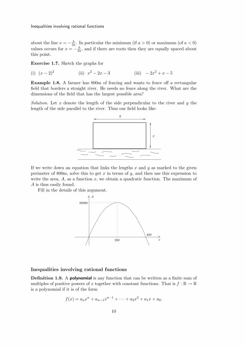
Example 1.8. A farmer has 800m of fencing and wants to fence off a rectangularfield that borders a straight river. He needs no fence along the river. What are thedimensions of the field that has the largest possible area?
Solution. Let x denote the length of the side perpendicular to the river and y thelength of the side parallel to the river. Thus our field looks like:
y
x
If we write down an equation that links the lengths x and y as marked to the givenperimeter of 800m, solve this to get x in terms of y, and then use this expression towrite the area, A, as a function x, we obtain a quadratic function. The maximum ofA is thus easily found.
Fill in the details of this argument.
A
200
400
80000
x
Inequalities involving rational functions
Definition 1.9. A polynomial is any function that can be written as a finite sum ofmultiples of positive powers of x together with constant functions. That is f : R → R
is a polynomial if it is of the form
f(x) = anxn + an−1xn−1 + · · · + a2x
2 + a1x + a0.
10

INEQUALITIES
If the constant an 6= 0 in the above then we say that f is of degree n. So a quadraticis a polynomial of degree 2.
A rational function is any function g that can be written as g(x) = p(x)/q(x) interms of two polynomials p and q.
So, for example, each of the functions fn(x) = xn that we considered above arepolynomials, where fn is of degree n. Similarly the following are all polynomials
x3 − 2x + 7; −2x7 + 3x6 − 5x4 − x3 + 2x2 + 17x − 1; x31 − x17
of degree 3, 7 and 31 respectively, whereas
x3 − x2 + 3x + 8
x5 + 7x4 − x2 + 9and
x12 − 9x9 + 7x5 + 2x
10x8 + 9x7 + 8x6 + 7
are both rational, but not polynomials. Note that the value of a polynomial functionis defined for all values of x since all we are doing is multiplying and adding numberstogether. The situation with rational functions is in general more complicated sincedivision has now come into play, and the denominator may be zero. For example wehave x3 + 2x2 − x − 2 = (x + 2)(x + 1)(x − 1)
⇒ x4 − x2
x3 + 2x2 − x − 2=
x4 − x2
(x + 2)(x + 1)(x − 1)
and so the function is not defined when x = −2, −1 or 1. Indeed, any polynomialof degree greater than 2 can be factorised into polynomials of lower degree accordingto:
Theorem 1.10 (Fundamental Theorem of Algebra). Any polynomial (over R)can be written as a product of polynomials of degree at most 2.
For example, our polynomial of degree 3 appearing in the denominator could bewritten as a product of polynomials of degree 1, each of which equals 0 for exactlyone value of x. On the other hand we have
x3 − 3x2 + x − 3 = (x − 3)(x2 + 1),
and the factor x2 + 1 cannot be broken up any further if we are to only use realcoefficients. Indeed, since x2 ≥ 0 for all x ∈ R we have x2 +1 ≥ 1, and so there are no(real) solutions to the equation x2 +1 = 0. Hence we cannot write it as (x−a)(x− b)for some a, b ∈ R. On the other hand, if we allow ourselves to use complex numbersthen we have x2 + 1 = (x − i)(x + i), where i2 = −1, and so
x3 − 3x2 + x − 3 = (x − 3)(x − i)(x + i).
Another version of the Fundamental Theorem of Algebra, in which coefficients androots are allowed to be chosen from the complex numbers C says that any polynomialin this setting can be written as a product of polynomials of degree 1.
We now discuss inequalities involving rational functions. So these functions in-volve a single real variable x, and given a particular value of x the inequality mayor may not be satisfied. The solution set of an inequality is the set of all of thosenumbers x that satisfy the inequality.
11

Inequalities involving rational functions
Example 1.11. Find the solution set for the inequality 3x + 5 > 8x − 10.
Solution. We have the chain of equivalences
3x + 5 > 8x − 10
⇔ 3x − 8x > −10 − 5 (by I3, with c = ±(−8x − 5))
⇔ −5x > −15 (evaluating)
⇔ −5x
−5<
−15
−5(mult. by 1
−5/−5, using I4)
⇔ x < 3 (evaluating)
Thus the equality we started with is satisfied if and only if x is less than 3, and sothe solution set is (−∞, 3).
Example 1.12. Find the solution set of the inequality
x2 ≤ 4x − 3 (†)
Solution. Here we can first use I3 to get
x2 ≤ 4x − 3 ⇔ x2 − 4x + 3 ≤ 0 ⇔ (x − 1)(x − 3) ≤ 0.
The factors are both of degree 1, hence both are equal to 0 for exactly one value ofx, and change sign at this point. The points where the product (x − 1)(x − 3) canchange sign are thus x = 1 and x = 3, and this quadratic will stay the same signand be nonzero in between these two values. The behaviour of (x − 1)(x − 3) is thussummarised by
x < 1 x = 1 1 < x < 3 x = 3 x > 3
x − 1 − 0 + + +
x − 3 − − − 0 +
(x − 1)(x − 3) + 0 − 0 +
Thus we see that (x− 1)(x − 3) ≤ 0 if and only if x ∈ [1, 3], and since this inequalityis equivalent to (†) it follows that this is also the solution set for (†).
����
������
��
����
�� ��������1 3
3
y
x
y = x2 − 3x + 4
12
INEQUALITIES
Exercise 1.13 (S02 1(a)). Find the solution set of the inequality
x + 3
x − 1<
x
x + 2(x 6= −2, 1) (∗)
and mark this set on a diagram.
Note. When doing this exercise using the method outlined in these notes you shouldend up with an inequality of the form f(x) > 0, and a number of points where thefunction f(x) can change sign. At such points f(x) will either equal 0 or be undefined,so certainly such points are not part of the solution set, and so separate columns forthem in your table are not required.
Another is that you should resist the temptation to multiply either side of (∗)by (x − 1)(x + 2) to get rid of the fractions. The reason for this is that the sign
of the number (x − 1)(x + 2) depends on the value of x, so we do not necessarilyknow if the number we are multiplying is positive or negative, and hence if we needto reverse the inequality symbol. One way to get round this problem is to treat thecases (x − 1)(x + 2) < 0 (when −2 < x < 1) and (x − 1)(x + 2) > 0 (when x < −2or x > 1) separately. Another would be to multiply by the nonnegative number(x − 1)2(x + 2)2. In both approaches one then needs to remember to exclude thepoints x = −2 and x = 1 from any solution set that may be discovered, since ouroriginal inequality does not make sense for these values of x.
Exercise 1.14 (S03 1(a)). Find the solution set of the inequality
x
x + 2≤ 3
x − 2
The modulus function; obtaining bounds
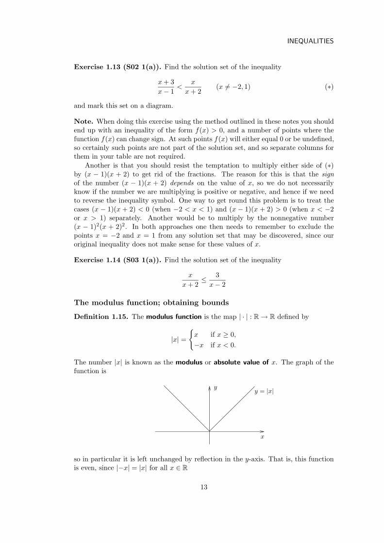
Definition 1.15. The modulus function is the map | · | : R → R defined by
|x| =
{x if x ≥ 0,
−x if x < 0.
The number |x| is known as the modulus or absolute value of x. The graph of thefunction is
y
x
y = |x|
so in particular it is left unchanged by reflection in the y-axis. That is, this functionis even, since |−x| = |x| for all x ∈ R
13

The modulus function; obtaining bounds
Basically the number |x| is what we get by ignoring the sign of x if it is negative.As a result, if we have the graph of some function y = f(x), then to draw the graphof the function y = |f(x)| we take the part lying below the x-axis and reflect it inthat line. The part lying above remains the same, since in this case f(x) ≥ 0, hence|f(x)| = f(x). For example, the graphs of sin x and | sin x| are:
y = sinx y = | sinx|
π
π−π −π2π 2π
−2π
−2π
Similarly the graphs of log x and | log x| are:
y = log x y = | log x|
The following are properties of |x| that we can prove easily from its definition:
Proposition 1.16. Let x, y ∈ R. Then
(i) |x|2 = x2; x ≤ |x|;∣∣∣∣1
x
∣∣∣∣ =1
|x| if x 6= 0.
(ii) |xy| = |x||y|.
(iii)
∣∣∣∣x
y
∣∣∣∣ =|x||y| if y 6= 0.
(iv) |x + y| ≤ |x| + |y|.
(v)∣∣|x| − |y|
∣∣ ≤ |x − y|.Proof. (i) Now |x| = ±x, so for the first part we have |x|2 = (±x)2 = x2. For theother two parts we split the proof into three cases. If x = 0 then |x| = x. If x > 0then |x| = x, and 1
x > 0, hence | 1x | = 1x = 1
|x| . If x < 0 then |x| > 0 > x, and 1x < 0,
hence | 1x | = − 1x = 1
−x = 1|x| .
(ii) For this note that
|xy|2 = (xy)2 = xy × xy = x2y2 = |x|2|y|2 = (|x||y|)2
14

INEQUALITIES
where we have used the first part of (i) a number of times. But |xy| ≥ 0 and |x||y| ≥ 0,so by Corollary 1.5 we can take (positive) square roots to get |xy| = |x||y| as required.
(iii) By (i) and (ii) we have |xy | = |x × 1y | = |x|| 1y | = |x| × 1
|y| = |x||y| .
(iv) We have
|x + y|2 = (x + y)2 = x2 + 2xy + y2 ≤ x2 + 2|xy| + y2 (by (i))
= |x|2 + 2|x||y| + |y|2 (by (i) and (ii))
= (|x| + |y|)2
However, both |x+y| ≥ 0 and |x|+ |y| ≥ 0, and so we can conclude from Corollary 1.5(by taking positive square roots) that |x + y| ≤ |x| + |y| as required.
(v) For this one note that by (iv) we get
|x| = |(x − y) + y| ≤ |x − y| + |y| ⇒ |x| − |y| ≤ |x − y|.
Similarly, by swapping the roles of x and y,
|y| − |x| ≤ |y − x| = |−(x − y)| = |x − y|
But∣∣|x| − |y|
∣∣ is equal to |x| − |y| or −(|x| − |y|) = |y| − |x|, and so we have shown
∣∣|x| − |y|∣∣ ≤ |x − y|
as required.
Now consider the inequality |x| < 7. To apply the definition of |x| in order to findthe solution set for this inequality we split the problem into two parts, depending onwhether x is in [0,∞) or (−∞, 0). So we have
if x ∈ [0,∞) and |x| < 7 then 0 ≤ x = |x| < 7
and if x ∈ (−∞, 0) and |x| < 7 then x < 0 and −x = |x| < 7 ⇒ −7 < x < 0.
Thus a number x ∈ R satisfies |x| < 7 if and only if −7 < x < 7, which is illustratedon the graph below:
����������������
��
y
x
y = |x|
y = 7
7−7
There was clearly nothing special about the choice of the number 7 in the abovecalculation. Indeed, for any positive number δ > 0 the solution set of the inequality|x| < δ is −δ < x < δ. Furthermore, we can use this to solve the following veryimportant inequality:
|x − a| < δ
15

The modulus function; obtaining bounds
where a ∈ R and δ > 0. Indeed, if we set y = x − a then |x − a| < δ becomes |y| < δwhich has solution set −δ < y < δ. But replacing y by x − a gives
−δ < x − a < δ ⇔ a − δ < x < a + δ.
This is shown graphically by
����������������
����
���������������������������������������������������
�������������������������������������������������
��������������������������������������������������
������������������������������
��������
��������
����������������
y
x
δ
a + δ a + δa − δ a − δ
y = |x − a|
a a
noting that the graph for y = |x − a| is got by shifting that for y = |x| to the rightby a units. Thus we see that a number x satisfies the inequality |x − a| < δ if andonly if it is in the interval (a − δ, a + δ), with centre point a and of width 2δ. Thatis, it satisfies the inequality if and only if its distance from the point a is less than δ.
One useful trick to solve inequalities involving absolute values is to recall that forany a, b ∈ [0,∞) we have a < b if and only if a2 < b2. Moreover, |x| ≥ 0 for all x ∈ R,and |x|2 = x2. These facts help us to remove the modulus signs, without having tosplit everything into several cases.
Example 1.17. Find the solution set of the inequality
∣∣∣∣2x + 5
x + 4
∣∣∣∣ ≥ 1 (x 6= −4) (∗)
Note that we have to exclude x = −4 in the above, since the fraction on the lefthand side is not defined for this value of x. Also, unlike before when we were dealingwith rational functions, we are now able to multiply by factors such as |x + 4|, sincethis number is nonnegative by definition.
Solution. We have the following equivalences (subject to x 6= −4):
∣∣∣∣2x + 5
x + 4
∣∣∣∣ =|2x + 5||x + 4| ≥ 1 (by (iii) of Proposition 1.16)
⇔ |2x + 5| ≥ |x + 4| (mult./div by |x + 4|)⇔ |2x + 5|2 ≥ |x + 4|2
⇔ 4x2 + 20x + 25 ≥ x2 + 8x + 16
⇔ 3x2 + 12x + 9 ≥ 0 (add/subtract −x2 − 8x − 16)
⇔ x2 + 4x + 3 ≥ 0 (mult./div. by 3)
⇔ (x + 3)(x + 1) ≥ 0
We thus see that the solution set of (∗) is (−∞,−4)∪ (−4,−3]∪ [−1,∞). [You couldproduce a table at this stage, but for solving a quadratic this may be excessive.]
16

INEQUALITIES
Exercise 1.18 (A02 1(a)). Find the solution set of the inequality
|x + 4| > |3x − 8|
and mark this set on a diagram.
When applying the definition of limits in the next chapter to particular examplesit is useful to find bounds for the growth of functions. That is given a function f(x)and some finite subinterval I ⊆ R, we would often like to find numbers M and/or Nsuch that
|f(x)| ≤ N or M ≤ |f(x)| ≤ N for all x ∈ I.
It turns out that for our applications we generally only need some crude choice for N ,rather than finding the best possible bound, and consequently the triangle inequality(part (iv) of Proposition 1.16) gives an efficient method. Indeed that says that
|x + y| ≤ |x| + |y|
for all x, y ∈ R. An induction argument applied to this gives
|x1 + x2 + · · · + xn| ≤ |x1| + |x2| + · · · + |xn|
for any n ≥ 1 and any xi ∈ R.
Exercise 1.19 (A04 3(b)). Find a positive number N > 0 such that∣∣∣∣x
3 − 3x cos x +4
x
∣∣∣∣ ≤ N
for all 1 ≤ x ≤ 3.
Example 1.20. Find positive numbers M and N such that M ≤∣∣∣∣x + 3
x − 2
∣∣∣∣ ≤ N for
all x ∈ [4, 7].
Solution. By (iii) of Proposition 1.16,∣∣∣∣x + 3
x − 2
∣∣∣∣ =|x + 3||x − 2| =
a
d
where a = |x + 3| and d = |x − 2|.Now 4 ≤ x ≤ 7 is equivalent to 7 ≤ x+3 ≤ 10, so for such x, |x+3| = x+3 ≤ 10.
Similarly 4 ≤ x ≤ 7 is equivalent to 2 ≤ x − 2 ≤ 5, and so |x − 2| = x − 2 ≥ 2 in thiscase. Now if we set b = 10 and c = 2, then we have a ≤ b = 10 and d ≥ c = 2 and soby (vi) of Proposition 1.1
a
d≤ b
c=
10
2= 5.
That is, ∣∣∣∣x + 3
x − 2
∣∣∣∣ ≤ 5
for all x ∈ [4, 7]. Hence N = 5 will do.
Exercise 1.21. Show that we can take M = 75 .
Exercise 1.22. Show that M must be no bigger than 2.
17

2 Limits and Continuity
The intuitive idea of limits
Our aim in this course is to give a rigorous introduction to the basic ideas of calculus,a branch of mathematics that has come to dominate the physical sciences. The mainunderlying concept in calculus is that of the limit — the behaviour of a function asthe point at which you evaluate it gets closer and closer to some prescribed value.Such ideas were finally developed with sufficient rigour in the 19th Century, longafter calculus had been invented in the 17th Century by Leibniz and Newton. Back
then statements such as f(x) → f(u) or limδx→0
δy
δxwere written down and dealt with
intuitively, but not fully explained. Indeed, the lack of clear definition or explanationoften lead the practitioners to draw incorrect conclusions! Here the number δx isused to denote a small change in the variable x, and in the limit people talked ofinfinitesimal numbers, which were sometimes assumed to be zero and sometimes not,according to what was convenient at that stage in a calculation for the particularauthor. . .
The goal of this section is give a precise definition of limit on which we canbuild the appropriate definition of the derivative of a function. We shall considerthe limiting behaviour of functions f : R → R, and begin by recalling the followingimportant result from the previous chapter: for any a ∈ R and δ > 0, the inequality|x − a| < δ is equivalent to the double inequality a − δ < x < a + δ, i.e. x lies in theinterval (a − δ, a + δ):
��������������������������
����
x
a + δa − δ a
Thus if f : R → R is a function and ε > 0 a given number, the statement that|f(x)− l| < ε is equivalent to l − ε < f(x) < l + ε, that is, f(x) ∈ (l − ε, l + ε). Notethat a is the midpoint of the interval (a−δ, a+δ) and l is the midpoint of the interval(l − ε, l + ε).
Example 2.1. Consider the function f : R → R defined by f(x) = x2.
2
4
y
y = x2
xx1 x2
y1
y2
4 + ε
4 − ε
2 + δ2 − δ
18

LIMITS AND CONTINUITY
Consider the point x = 2, mapped by the function f to 22 = 4. Choose a smallpositive number ε > 0, which should be thought of as the acceptable degree of error,and consider the interval (4−ε, 4+ε) about 4, i.e. the set of all y such that |y−4| < ε.
Now put x1 =√
4 − ε and x2 =√
4 + ε. Recall that f(x) = x2 is strictly increas-ing on [0,∞) by Proposition 1.4, hence x1 < 2 < x2. Furthermore
x1 < x < x2 ⇒ x21 = 4 − ε < x2 = f(x) < 4 + ε = x2
2 ⇒ |f(x) − 4| < ε. (†)
Since x1 < 2 < x2, if we define δ = 12 min{2 − x1, x2 − 2} then in particular δ > 0.
Also, if |x − 2| < δ then 2 − δ < x < 2 + δ. But
δ ≤ 12 (2 − x1) ⇒ 2 − δ ≥ 2 − 1
2(2 − x1) > 2 − (2 − x1) = x1, and
δ ≤ 12 (x2 − 2) ⇒ 2 + δ ≤ 2 + 1
2(x2 − 2) < 2 + (x2 − 2) = x2.
Thus if |x − 2| < δ then x1 < x < x2, and so 4 − ε < x2 < 4 + ε by (†). That is
0 < |x − 2| < δ ⇒ |f(x) − 4| < ε.
To give an example of possible values that ε and δ might take, consider settingε = 0.1. Then x1 =
√3.9 ≈ 1.975, and x2 =
√4.1 ≈ 2.025, and so 2 −
√3.9 ≈ 0.025
and√
4.1 − 2 ≈ 0.025. Thus if we set δ = 0.012 ≈ 12 × 0.025, then 2 − δ = 1.988 and
2 + δ = 2.012. So now if we choose any x satisfying 0 < |2 − x| < 0.012, we will have|f(x) − 4| < 0.1.
Similarly if we take ε = 0.01 then x1 =√
3.99 ≈ 1.9975 and x2 =√
4.01 ≈ 2.0025.Thus if we set δ = 0.0012 ≈ 1
2 × 0.0025 then 2 − δ = 1.9988 and 2 + δ = 2.0012, andif we choose any x satisfying 0 < |2 − x| < 0.0012, we will have |f(x) − 4| < 0.01.
The important point about our calculations with ε and δ above is that no matter
how small a value of ε we choose there is always some δ > 0 for which
0 < |x − 2| < δ ⇒ |f(x) − 4| < ε.
For instance it will work for ε = 0.001, 0.0000001, . . . As the value of ε gets smallerand smaller, we will need to choose smaller and smaller values of δ, forcing x to becloser and closer to 2, but it is always possible to find this δ. And by choosing smallerand smaller ε we are ensuring that f(x) is as close as we like to 4.
Anticipating the definition below, we write the conclusion of the above as
limx→2
f(x) = 2, or f(x) → 4 as x → 2.
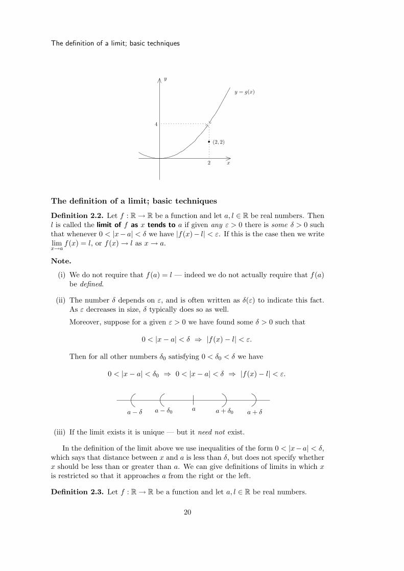
It is true that 4 = 22 = f(2), but that is not actually relevant to the abovediscussion. Indeed above we wrote the double inequality 0 < |x − 2| < δ, whichimplies in particular that x 6= 2, i.e. x does not actually take the value 2, but merelyapproaches it. So if we were to define a new function g : R → R by
g(x) =
{x2 if x 6= 2,
2 if x = 2,
then the same calculations would apply, and we could conclude that limx→2
g(x) = 4,
even though g(2) = 2 6= 4.
19
The definition of a limit; basic techniques
2
(2, 2)
4
y
y = g(x)
x
The definition of a limit; basic techniques
Definition 2.2. Let f : R → R be a function and let a, l ∈ R be real numbers. Thenl is called the limit of f as x tends to a if given any ε > 0 there is some δ > 0 suchthat whenever 0 < |x− a| < δ we have |f(x)− l| < ε. If this is the case then we writelimx→a
f(x) = l, or f(x) → l as x → a.
Note.
(i) We do not require that f(a) = l — indeed we do not actually require that f(a)be defined.
(ii) The number δ depends on ε, and is often written as δ(ε) to indicate this fact.As ε decreases in size, δ typically does so as well.
Moreover, suppose for a given ε > 0 we have found some δ > 0 such that
0 < |x − a| < δ ⇒ |f(x) − l| < ε.
Then for all other numbers δ0 satisfying 0 < δ0 < δ we have
0 < |x − a| < δ0 ⇒ 0 < |x − a| < δ ⇒ |f(x) − l| < ε.
a + δa − δ a + δ0a − δ0a
(iii) If the limit exists it is unique — but it need not exist.
In the definition of the limit above we use inequalities of the form 0 < |x−a| < δ,which says that distance between x and a is less than δ, but does not specify whetherx should be less than or greater than a. We can give definitions of limits in which xis restricted so that it approaches a from the right or the left.
Definition 2.3. Let f : R → R be a function and let a, l ∈ R be real numbers.
20

LIMITS AND CONTINUITY
(i) l is called the left limit of f as x tends to a if given any ε > 0 there is some
δ > 0 such that whenever 0 < a− x < δ we have |f(x)− l| < ε. This is writtenlim
x→a−f(x) = l, or f(x) → l as x → a−.
(ii) l is called the right limit of f as x tends to a if given any ε > 0 there is some
δ > 0 such that whenever 0 < x− a < δ we have |f(x)− l| < ε. This is writtenlim
x→a+f(x) = l, or f(x) → l as x → a+.
Note that for the left limit to exist we must have 0 < a−x < δ, which is equivalentto saying that a − δ < x < a, that is x is less than a, and so must “approach fromthe left”. Similarly, for the right limit to exist we must have a < x < a + δ, and so x“approaches from the right.”
Proposition 2.4. Let f be a function R → R and a ∈ R. Then limx→a
f(x) exists if
and only if limx→a−
f(x) and limx→a+
f(x) both exist and are equal.
Example 2.5. Define f : R → R by
f(x) =
{2 if x ≥ 0,
1 if x < 0.
This has graph
y
x
1
2
and so pictorially we see that limx→0+
f(x) = 2 and limx→0−
f(x) = 1. Thus the left and
right limits exist, but they are unequal. Hence limx→0
f(x) does not exist.
Example 2.6. Let c and d be any two real numbers. Using the definition of limitsshow that if f(x) = c+dx for all x ∈ R then for each a ∈ R we have lim
x→af(x) = c+da.
Solution. For each x ∈ R and the specified point a ∈ R we have
|f(x) − (c + da)| = |c + dx − c − da| = |d(x − a)| = |d||x − a|. (∗)
Case 1. d = 0: In this case, if we choose any positive number ε > 0 then by (∗)
|f(x) − c| = |0||x − a| = 0 < ε
for every x ∈ R. Thus if we choose any positive number δ > 0 then
0 < |x − a| < δ ⇒ |f(x) − c| < ε,
21

The definition of a limit; basic techniques
and so limx→a
f(x) = c as required.
Case 2. d 6= 0: Again choose some ε > 0, and now set δ = ε|d| > 0. Then by (∗)
0 < |x − a| < δ ⇒ |f(x) − (c + da)| < |d|δ = |d| × ε
|d| = ε,
and so limx→a
f(x) = c + da as required.
Example 2.7. Using the ε-δ definition of a limit, show that limx→2
(x2 + 5x − 7) = 7.
Solution. For convenience, define f to be the function f(x) = x2 + 5x− 7 and choosean ε > 0. We must find some δ > 0 such that if 0 < |x − 2| < δ, then |f(x) − 7| < ε.Now
|f(x) − 7| = |(x2 + 5x − 7) − 7| = |x2 + 5x − 14| = |(x + 7)(x − 2)| = |x + 7||x − 2|
and so if we choose any δ > 0, then whenever 0 < |x − 2| < δ we will have
|f(x) − 7| ≤ δ|x + 7|
But what is |x + 7| less than? Well we are only really interested in values of x closeto 2, so we can always make an initial restriction on δ, say by requiring that it isless than 1. So then if |x − 2| < δ with such a δ, then we have restricted x to liein (2 − δ, 2 + δ), and this interval is itself contained in (2 − 1, 2 + 1) = (1, 3) by theassumption on δ. But if x ∈ (1, 3) then 8 = 1+7 < x+7 < 3+7 = 10. So restrictingδ to be less than 1 tells us that if |x− 2| < δ then we must have |x + 7| = x + 7 < 10.
So now choose δ = min{12 , ε
10}. Then 0 < δ < 1 (which is why we used 12 in its
definition), and whenever 0 < |x − 2| < δ we have, since δ ≤ ε10 ,
|f(x) − 7| ≤ δ|x + 7| ≤ ε
10|x + 7| <
ε
10× 10 = ε.
Thus we have that limx→2
(x2 + 5x − 7) = 7.
The above result is not overly easy to prove, certainly not as easy as it was to provethe limits in Example 2.6. However that earlier example, together with the followingproposition, give a much faster route to proving the above result. The proofs givenillustrate the need for, and an application of, the rigorous definition of limits.
Proposition 2.8 (Calculus of Limits). Suppose that f and g are two functions
R → R, and that for some a ∈ R we have
limx→a
f(x) = p, and limx→a
g(x) = q
for some p, q ∈ R. Then
(i) limx→a
(f(x) + g(x)
)= p + q.
(ii) limx→a
(f(x)g(x)
)= pq.
22

LIMITS AND CONTINUITY
(iii) If q 6= 0, then limx→a
f(x)
g(x)=
p
q.
(iv) If n is any positive integer and p > 0 then limx→a
n
√f(x) = n
√p.
Proof. (i) Fix an ε > 0, then ε2 > 0 as well. Since lim
x→af(x) = p and lim
x→ag(x) = q
there are positive numbers δf > 0 and δg > 0 such that
0 < |x − a| < δf ⇒ |f(x) − p| <ε
2, and
0 < |x − a| < δg ⇒ |g(x) − q| <ε
2.
Now if we define δ = min{δf , δg} then δ > 0. Moreover if 0 < |x − a| < δ then0 < |x − a| < δf and 0 < |x − a| < δg, and so by the inequalities above we have
|(f(x) + g(x)) − (p + q)| = |(f(x) − p) + (g(x) − q)|≤ |f(x) − p| + |g(x) − q| <
ε
2+
ε
2= ε.
(iii) Fix an ε > 0, and assume that p 6= 0. Set
εf =ε|q|4
> 0, and εg = min
{ε|q|24|p| ,
|q|2
}> 0.
By hypothesis there are positive numbers δf > 0 and δg > 0 such that
0 < |x − a| < δf ⇒ |f(x) − p| < εf , and
0 < |x − a| < δg ⇒ |g(x) − q| < εg.(†)
By the reverse triangle inequality (part (v) of Proposition 1.16) we have
|g(x)| =∣∣q −
(q − g(x)
)∣∣ ≥ |q| − |q − g(x)|
and so if 0 < |x − a| < δg then |g(x) − q| < εg ≤ 12 |q|, and hence
|g(x)| ≥ |q| − 12 |q| = 1
2 |q| > 0. (‡)
Define δ = min{δf , δg}, so in particular δ > 0. Now
f(x)
g(x)− p
q=
q(f(x) − p
)− p
(g(x) − q
)
qg(x).
Thus if 0 < |x − a| < δ, then the inequalities (†) and (‡) both hold and so
∣∣q(f(x) − p
)− p
(g(x) − q
)∣∣ ≤ |q||f(x) − p| + |p||g(x) − q|< |q|εf + |p|εg
≤ |q| × ε|q|4
+ |p| × ε|q|24|p| =
ε|q|22
and|qg(x)| = |q||g(x)| ≥ 1
2 |q|2.
23
The definition of a limit; basic techniques
So, finally, by part (vi) of Proposition 1.1 we have
0 < |x − a| < δ ⇒∣∣∣∣f(x)
g(x)− p
q
∣∣∣∣ <12ε|q|212 |q|2
= ε
as required.If p = 0 then setting εf = 1
2ε|q| and εg = 12 |q| at the outset of the proof, and
following the same steps, will yield the desired result.
Example 2.9. Show that limx→a
x2 = a2 for any real number a ∈ R.
Solution. To show this, let g : R → R be the function g(x) = x, then limx→a
g(x) = a as
shown in Example 2.6 (taking c = 0, d = 1). Now note that f(x) = x2 = g(x)g(x),so by part (ii) of Proposition 2.8 we have
limx→a
f(x) = limx→a
(g(x)g(x)
)=
(limx→a
g(x))(
limx→a
g(x))
= a × a = a2.
Exercise 2.10 (A02 1(b)). Use the calculus of limits to evaluate the following:
limx→0
x3 + x2 − 5x + 3
x2 + x − 2, lim
x→1
x3 + x2 − 5x + 3
x2 + x − 2
Example 2.11. Find the limit limx→−1
√2 + x − 1
x + 1.
Solution. A direct use of the calculus of limits to top and bottom gives the meaninglessanswer 0
0 , as would happen in the exercise above. So note that
√2 + x − 1
x + 1=
√2 + x − 1
x + 1×
√2 + x + 1√2 + x + 1
(x 6= −1)
=(2 + x) − 1
(x + 1)(√
2 + x + 1)=
x + 1
(x + 1)(√
2 + x + 1)
=1√
2 + x + 1.
So now by Proposition 2.8(iii) and (iv) (with n = 2) we have
limx→−1
√2 + x − 1
x + 1=
1
limx→−1
(√
2 + x + 1)=
1
2.
Exercise 2.12 (A04 1(b ii)). Use the calculus of limits to evaluate the following:
limx→2
√2x − 3 −
√x − 1
x − 2
In Examples 2.10, 2.11 and 2.12 above we made use of the following fact:
Proposition 2.13. Suppose that f and g are functions for which f(x) = g(x) for all
x 6= a. If limx→a
f(x) exists then so does limx→a
g(x), and moreover limx→a
f(x) = limx→a
g(x).
24
LIMITS AND CONTINUITY
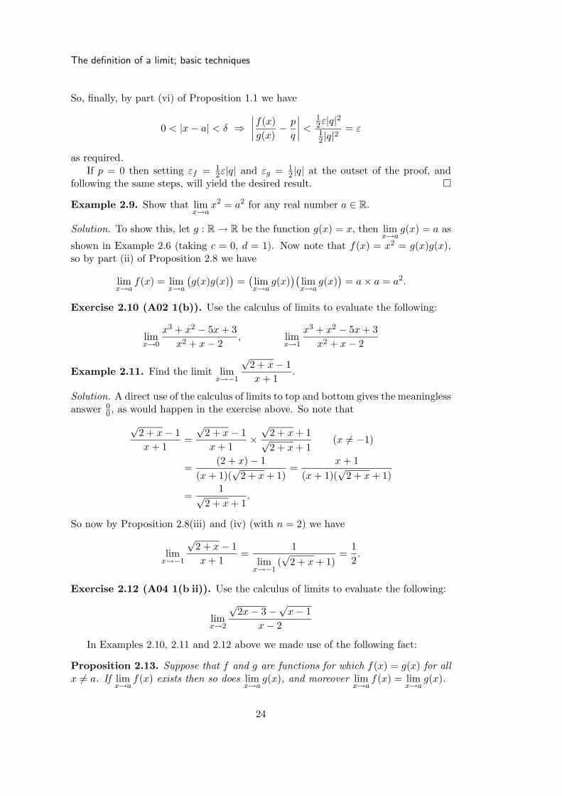
Example 2.14. limx→0
sin x
x= 1 and lim
x→0
cos x − 1
x= 0.
These limits involving trigonometric functions are important for the calculationof the derivatives of sin x and cos x, and can be proved geometrically by consideringa circle of radius 1, and the sector cut off by an angle of x radians:
x
A
BCDO
OA and OC are both of length 1, so the perpendicular height OD of triangle △OACis sinx, and thus its area is 1
2 × 1 × sinx = 12 sinx. Similarly AB has length tan x,
since OAB is a right-angle, and thus △OAB has area 12 tan x. Between these two
triangles is the sector OAC, whose area is x2π × π × 12 = 1
2x, and so we have
area of △OAC < area of sector OAC < area of △OAB
⇒ 12 sin x < 1
2x < 12 tan x =
sin x
2 cos x
⇒ 1 <x
sin x<
1
cos x.
But from the graph of cosx we know that cos x → 1 as x → 0, so 1cos x → 1 as x → 0
by the calculus of limits. This forces xsinx → 1 as x → 0, and so sinx
x → 1 as x → 0 asstated.
For the other limit we have
cos x − 1
x=
cos x − 1
x× cos x + 1
cos x + 1=
cos2 x − 1
x(cos x + 1)
=− sin2 x
x(cos x + 1)= −sin x
x× sin x
cos x + 1
We know already that limx→0
sin x
x= 1. Moreover lim
x→0sin x = 0 and lim
x→0(cos x + 1) =
1 + 1 = 2, so that
limx→0
sinx
cos x + 1=
0
2= 0 ⇒ lim
x→0
cos x − 1
x= −1 × 0 = 0.
So far all but one of our functions have had limits at the given point(s), andthe badly behaved one in Example 2.5 at least had (differing) left and right limits.However there are functions whose behaviour is far worse.
25

The definition of a limit; basic techniques
Example 2.15. limx→0
1
xdoes not exist.
To see this consider the graph of 1x :
y
x
M
−M
1
M
− 1
M
y = 1
x
As x approaches 0 from the right 1x becomes very large and positive, and as x
approaches 0 from the left 1x becomes very large and negative. More formally, if we
choose any M > 0 then
0 < x <1
M⇒ 1
x> M and − 1
M< x < 0 ⇒ 1
x< −M
That is 1x becomes greater (or less) than any bound M (−M) we choose for all values
of x sufficiently close to 0.
We say that limx→0
1
xdoes not exist because the function diverges or blows up at
the origin. Other functions fail to have limits despite not blowing up at the point ofinterest:
Example 2.16. limx→0
f(x) does not exist for f : R → R defined by
f(x) =
{1 if x = 1
n for some n ≥ 1,
0 otherwise.
To see this note that for any choice of δ > 0 there are values of x satisfying 0 < x < δfor which f(x) = 1 (take any x = 1
n for n > 1δ ) and values of x for which f(x) = 0.
Thus f(x) cannot approach a single value as x → 0+.Note however that f(x) = 0 for all x < 0, and so lim
x→0−f(x) = 0.
1
11
2
1
3
1
4
y
x
26
LIMITS AND CONTINUITY
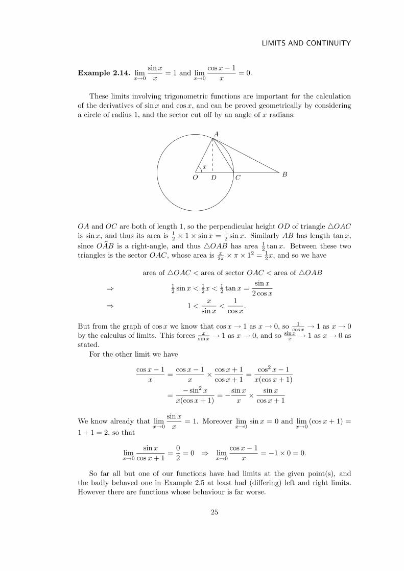
Coping with infinity
Consider the function f(x) = 1x2 . We can obtain a sketch the graph of this function
by looking at the graph for x 7→ x2:
yy
y = x2 y = 1
x2
x
x
The function blows up at x = 0 but unlike 1x it goes to +∞ as x converges to
0 from either side. Moreover, note that as x gets very large, in either direction,the value of 1
x2 is always positive but gets closer and closer to 0. The notation anddefinitions for these sorts of behaviour are as follows:
Definition 2.17. Let f be a function on R and a ∈ R. Then f diverges to infinity
as x tends to a if for every M > 0 there is some δ > 0 such that
0 < |x − a| < δ ⇒ f(x) > M.
This is written f(x) → +∞ as x → a.Similarly, f diverges to minus infinity as x tends to a if for every M > 0 there
is some δ > 0 such that
0 < |x − a| < δ ⇒ f(x) < −M,
and this is written f(x) → −∞ as x → a.
We can adjust the definition accordingly to take care to left and right limits, andwhen we do this can give meaning to the statements 1
x → +∞ as x → 0+, and1x → −∞ as x → 0−. Indeed, this was proved in Example 2.15.
For the limit of a function as the variable x gets large, the appropriate definitionsare as follows:
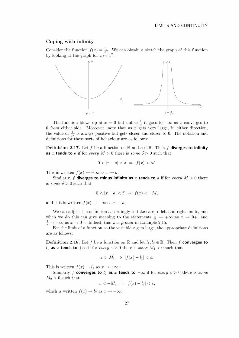
Definition 2.18. Let f be a function on R and let l1, l2 ∈ R. Then f converges to
l1 as x tends to +∞ if for every ε > 0 there is some M1 > 0 such that
x > M1 ⇒ |f(x) − l1| < ε.
This is written f(x) → l1 as x → +∞.Similarly f converges to l2 as x tends to −∞ if for every ε > 0 there is some
M2 > 0 such thatx < −M2 ⇒ |f(x) − l2| < ε,
which is written f(x) → l2 as x → −∞.
27
Coping with infinity
y
xM1
l1
l1 + ε
l1 − ε
If we combine elements of the two definitions we can then give a rigorous meaningto statements such as “f(x) → +∞ as x → +∞”.
Example 2.19.
(a) For each n ≥ 1 let fn(x) = xn for each x ∈ R. Then (recalling Proposition 1.4)
fn(x) → +∞ as x → +∞fn(x) → −∞ as x → −∞ if n is odd
fn(x) → +∞ as x → −∞ if n is even
That this is the case follows since fn(x) ≥ x for all x ≥ 1, and if x > 0 then
(−x)n = (−1)nxn =
{xn if n is even,
−xn if n odd.
(b) Let
f(x) =x − 3
x2 + 3x + 2.
Now x2 + 3x + 2 → (−1)2 + 3 × (−1) + 2 = 0 as x → −1 by the calculus oflimits, and x− 3 → (−1)− 3 = −4 6= 0. Moreover x2 + 3x + 2 = (x + 1)(x + 2),so
− 1 < x < 3 ⇒ x2 + 3x + 2 > 0 and x − 3 < 0 ⇒ f(x) < 0, and
− 2 < x < −1 ⇒ x2 + 3x + 2 < 0 and x − 3 < 0 ⇒ f(x) > 0.
It follows that
f(x) → +∞ as x → −1−, and f(x) → −∞ as x → −1 + .
For the behaviour as x → ±∞, divide top and bottom by x2. This gives
f(x) =x − 3
x2 + 3x + 2=
1x − 3
x2
1 + 3x + 2
x2
→ 0
1= 0
as x → +∞ and as x → −∞, since 1xn
→ 0 as x → ±∞ for each n ≥ 1.
Exercise 2.20. Carry out a similar analysis as done for f in part (b) of Example 2.19
above for the functions g(x) =x5 − 4x2 + 2
5 + 2x4 − 7x5and h(x) =
x2 − x + 1
x − 2.
28
LIMITS AND CONTINUITY
Continuous functions
The intuitive idea of a continuous function is one whose graph has ‘no jumps’, or ‘canbe drawn without taking the pen off of the paper.’ Consequently it should have alimit at each point a, that is f(x) should converge to some value as x tends to a, andfurthermore that value should be equal to the value of the function at that point.This idea is captured by the following:
Definition 2.21. Let f : R → R be a function and let a ∈ R. We say that f is
continuous at the point a if
(i) limx→a
f(x) exists, and
(ii) limx→a
f(x) = f(a).
f is continuous on R if it is continuous at every point a ∈ R.A function that is not continuous at a point a is called discontinuous. Intuitively
speaking it has a break in the graph at this point.
If we rewrite this using the definition of limits, we see that a function f : R → R
is continuous at a point a if for every choice of ε > 0 there is some δ > 0 such that
0 < |x − a| < δ ⇒ |f(x) − f(a)| < ε.
Now we must insist that f is defined at the point x = a unlike when we were con-sidering limits earlier, and since |f(x) − f(a)| = 0 when x = a, we can remove theinequality 0 < |x − a| from the definition. Thus the function is continuous at a if forevery ε > 0 there is some δ > 0 such that
|x − a| < δ ⇒ |f(x) − f(a)| < ε.
Example 2.22. For every choice of c, d ∈ R we know that the function f(x) = c+dxis continuous since by Example 2.6 we have that lim
x→af(x) = c + da = f(a).
Again, this one result in conjunction with the calculus of limits can be used togive many more examples of continuous functions.
Proposition 2.23. If f(x) and g(x) are functions R → R that are continuous at
x = a, then so are the functions f(x)+ g(x) and f(x)g(x). Moreover if g(a) 6= 0 then
the functionf(x)g(x) is continuous at x = a, as is the function n
√f(x) for each n ≥ 2 if
f(a) > 0.
Proof. These are all immediate consequences of the calculus of limits, as given inProposition 2.8. For instance, consider the function fg which maps the point x tof(x)g(x). Since f and g are continuous at a, f and g have limits there, and moreover
limx→a
f(x) = f(a), limx→a
g(x) = g(a).
Thus, by Proposition 2.8, limx→a
(f(x)g(x)
)exists, and is equal to the product of the
above limits, hence equals f(a)g(a) = (fg)(a) as required.
29

Continuous functions
Since any polynomial can be written as a sum of products of the functions con-sidered in Example 2.22, the above result leads immediately to the following:
Corollary 2.24. Every polynomial is continuous on R. Every rational function is
continuous wherever it is defined.
Definition 2.25. Let f and g be functions from R to R. Their composition is thefunction g ◦ f : R → R is defined by
(g ◦ f)(x) = g(f(x)
).
That is, apply f to the point x and then apply g to the result.
Example 2.26. Consider the functions f : R → R and g : R → R given by f(x) =x2 + 3 and g(x) = 1 − x. Calculate f ◦ g(x) and g ◦ f(x).
Note in particular that f ◦ g and g ◦ f are different functions in this example; thisis usually the case for compositions.
Proposition 2.27. Let f and g be functions R → R with f continuous at some point
a, and g continuous at the image point f(a). Then g ◦ f is continuous at a.
Proof. For each ε > 0 we must show that there is a δ > 0 such that
|x − a| < δ ⇒ |(g ◦ f)(x) − (g ◦ f)(a)| < ε.
So fix an ε > 0, then since g is continuous at the point f(a), there is some δg > 0such that
|t − f(a)| < δg ⇒ |g(t) − g(f(a))| < ε. (∗)
But in turn we know that f is continuous at a, so given this positive number δg > 0we know that there is some δ > 0 such that
|x − a| < δ ⇒ |f(x) − f(a)| < δg. (†)
So if we take any x ∈ R that satisfies |x − a| < δ then |f(x)− f(a)| < δg by (†). Butthis means that we can apply (∗) with t = f(x) to get
|x − a| < δ ⇒ |f(x) − f(a)| < δg ⇒ |g(f(x)) − g(f(a))| < ε,
which is precisely what we needed to show.
So far we have only considered continuous functions that have been defined atevery point of R. This may not always be the case, as in the following examples.
Example 2.28. Define a function f on R by
f(x) =x2 − 9
x − 3, x 6= 3.
Since x2 −9 = (x−3)(x+3) we have that f(x) = x+3 for all x 6= 3, and so for a 6= 3we have lim
x→af(x) = a + 3 = f(a), hence f is continuous at every a 6= 3.
30

LIMITS AND CONTINUITY
Moreover by Proposition 2.13 and Example 2.6 limx→3
f(x) = 6. So if we were
to extend the domain of definition of f by setting f(3) = 6 then we will obtain acontinuous function.
On the other hand if we define f to be any other value at x = 3 then it would stillbe true that f(x) → 6 as x → 3, but the redefined function will not be continuous inthis case since we will have f(3) 6= 6.
Example 2.29. The function f(x) = 1x is discontinuous at x = 0 since we have
shown that limx→0
f(x) does not exist.
Similarly consider the function g defined on all of R by
g(x) =
1
(x − 2)2if x 6= 2,
5 if x = 2.
As x tends to 2 we see that (x−2)2 converges to 0 and is positive, and so f(x) divergesto +∞. Hence lim
x→2f(x) cannot exist, and so f is not continuous at 2, despite the
fact that it is defined. Moreover, any change in the definition of f at x = 2 will notalter this fact.
2
5
yy = g(x)
x
The behaviour in Example 2.28 is different from that in Example 2.29. In thecase of Example 2.28 the point x = 3 is known as a removable discontinuity sincethe function does have a limit there, and so redefining the function will produce acontinuous function. In the case of Example 2.29 the points of discontinuity of f andg are essential discontinuities since they do not have limits, and so no matter howwe define the functions at these points, they will never be continuous there.
Another example of a removable discontinuity is the following:
Example 2.30. Let f be the function R → R defined by
f(x) =
{1 if x 6= 1,
2 if x = 1.
Then limx→1
f(x) = 1 6= f(1), and so f is not continuous at x = 1. If we redefine f to
31

Continuity on intervals
be 1 at x = 1 then we will remove the singularity.
y
x
1
2
2
Exercise 2.31 (S03 2(b)). Consider the following function on the real line R:
f(x) =x2 − 5x − 14
2x2 + 3x − 2
At which point(s) is f continuous? At which point(s) is f undefined?Determine whether the point(s) at which f is undefined are essential or removable
singularities.Describe the behaviour of f(x) as x → +∞
Continuity on intervals
Often a function may be defined only on some interval I of the real line and in thiscase we must make some changes to our definition of continuity. If a ∈ I is not anendpoint then x can approach a from either side and so it still makes sense to ask iff(a) = lim
x→af(x). If a ∈ I is an endpoint then x can only approach this value from one
side and still be in I, and so we must use one sided limits in our modified definitionof continuity.
Thus if I = [c, d] for some c < d, then a function f : I → R is continuous on I ifit is continuous at each point of I, which means that at a point a ∈ I
limx→a
f(x) exists and is equal to f(a) if c < a < d,
limx→a+
f(x) exists and is equal to f(a) if a = c, and
limx→a−
f(x) exists and is equal to f(a) if a = d.
Again, this just means that the graph has no breaks over [c, d].
y
xc d
leftrightlimit limit
here here
32

LIMITS AND CONTINUITY
A moments thought shows that if we start with a function that is continuous onall of R and restrict it so that we only consider values of x from some subintervalI then that function will also be continuous. This idea provides a ready supply ofcontinuous functions on subintervals of R to which we can apply the following result.
Theorem 2.32 (Intermediate Value Theorem). Let c, d ∈ R with c < d, and let
f : [c, d] → R be continuous. Then there are points x1, x2 ∈ [c, d] such that
f(x2) ≤ f(x) ≤ f(x1) for all x ∈ [c, d].
Moreover f takes all values between f(x2) and f(x1). That is, if y ∈ R satisfies
f(x2) ≤ y ≤ f(x1) then there is some x ∈ [c, d] such that f(x) = y.
The number f(x1) is called the maximum of f on [c, d] and the number f(x1) iscalled the minimum of f on [c, d]. The result is intuitively obvious, but not so easyto prove. It depends on the completeness of the real number system.
y
xc dx1
x2
f(x1)
f(x2)
Thus we see that any continuous function on an interval of the form [c, d] isbounded, that is the values f(x) that the function takes for x ∈ [c, d] lie between twonumbers. Conversely if we have an unbounded function g on [c, d], it follows that itcannot be continuous on [c, d].
Also, the Intermediate Value Theorem is not valid if we replace the interval [c, d]with any of the other three intervals having c and d as end points. For examplethe function f(x) = 1
x is well-defined and continuous on the open interval (0, 1) byTheorem 2.23. However f(x) → +∞ as x → 0+: there is no number M such thatf(x) ≤ M for all x ∈ (0, 1). Also f(x) > 1 for all x ∈ (0, 1) and lim
x→1f(x) = 1, so that
f(x) gets as close to 1 as we like. But there is no point x ∈ (0, 1) for which f(x) = 1.
One thing that the Intermediate Value Theorem can tell us is if there is a solutionto a given equation in a given interval. For instance consider the polynomial f(x) =x5 − 2x2 + 4x − 2. Then f is continuous on the interval [0, 1], since it is continuouson all of R. Moreover f(0) = −2 and f(1) = 1. Thus there must be some x0 ∈ (0, 1)such that f(x0) = 0 since f(x) assumes all values between −2 and 1, and so there is asolution to x5−2x2 +4x−2 = 0 in this interval. Unlike the case of quadratics, cubicsand quartics, there is no formula for finding the roots of quintics (and polynomials ofhigher degree), and so reasoning like the above gives a first step to locating them.
This use of the Intermediate Value Theorem also has a similar, but more theoret-ical application.
33
Continuity on intervals
Proposition 2.33. Let n ≥ 1 be an integer and a ≥ 0 any real number. There exists
a unique real number b ≥ 0 that satisfies bn = a; that is, there is a unique positive
nth root of a.
Proof. Recall from Proposition 1.4 that the function f : [0,∞) → R given by f(x) =xn is strictly increasing, and is a polynomial hence continuous. Moreover we knowthat f(x) → +∞ as x → ∞ (cf. part (a) of Example 2.19). In particular there mustbe some c > 0 such that f(c) = cn > a. Thus, by the Intermediate Value Theorem,f restricted to the interval [0, c] must take all values between f(0) = 0 and f(c) > a,and so there must be some b ≥ 0 that satisfies f(b) = bn = a. That is, there is an
nth root. That it is unique follows from the fact that f is strictly increasing, since ifd ≥ 0 such that d 6= b then either d < b or d > b, and in either case f(d) 6= f(b).
34

DIFFERENTIATION
3 Differentiation
The idea and definition of derivatives
Consider a distance-time graph for some object (car, bicycle, atom,. . . ) moving in a‘continuous manner’ through ‘one-dimensional space’. We plot the displacement fromthe starting point as a function of time, starting at t = 0.
d
t
d = f(t)
t1 t2
t2 − t1
f(t2) − f(t1)
t′2
A1
A2
A′2
Thus the function d = f(t) is continuous. The average velocity V (t1, t2) of our bodyas t varies from time t1 to time t2 is given by
V (t1, t2) =f(t2) − f(t1)
t2 − t1= slope of the line segment A1A2.
If we set h = t2 − t1, so that t2 = t1 + h, this can be rewritten as
V (t1, t2) =f(t1 + h) − f(t1)
h.
Here h is the ‘change in time’. We could also take the second time to be t′2, an earliertime than t1. That is t′2 < t1, which is equivalent to saying that h = t′2 − t1 < 0. Butin either case as we take smaller and smaller values of h (i.e. as h tends to 0), we hopethat this number will converge to a limit that we can call the actual or instantaneous
velocity at time t = t1.
We are trying to approximate the possibly complicated curve d = f(t) by astraight line at each point, that is, find the slope of the straight line that just touchesthe curve d = f(t) at the point (t1, f(t1)). Thus this straight line should meet thecurve at this point and go in the same direction — it is the tangent to the curve.
Definition 3.1. A function f : R → R is differentiable at a ∈ R if
limh→0
f(a + h) − f(a)
hexists.
The value of this limit is the derivative of f at a and is denoted f ′(a). The functionf is differentiable on R if it is differentiable at every a ∈ R. If this is the case, thenf ′ : a 7→ f ′(a) is a new function R → R.
35

The idea and definition of derivatives
Remarks. (i) Some authors will write
f ′(a) = lim∆a→0
f(a + ∆a) − f(a)
∆a(when it exists)
where ∆a stands for the change in the variable aAlso, often people use notation of the form y = f(x) for a function, in which case
if y (or f) is differentiable everywhere then the function f ′ is denoteddy
dx(ii) When defining the derivative we choose a function f and a point a, and from
these construct a new function g in the variable h by
g(h) =f(a + h) − f(a)
h
for all h 6= 0. Note that g depends on the variable h. We then ask if limh→0
g(h) exists.
The derivative cannot be calculated by substituting h = 0 or ∆a = 0 directly intothese formulae. It is for this reason that our definition of a limit of a function g(x)as x tends to some number b did not actually depend on g(b), and indeed did notrequire that this even be defined.
Since we hope to use the derivative to find straight line approximations to morecomplicated curves, we ought to check that it behaves correctly if we consider astraight line.
Proposition 3.2. Let c, d ∈ R and define f : R → R by f(x) = c + dx. Then f is
differentiable on R with f ′ : R → R given by f ′(x) = d for all x ∈ R. That is, the
derivative at each point is equal to the gradient of this straight line.
Proof. Choose an x ∈ R, then for any h 6= 0
f(x + h) − f(x)
h=
[c + d(x + h)] − [c + dx]
h
=dh
h= d
and so clearly
limh→0
f(x + h) − f(x)
h= d.
Thus the limit exists for all x ∈ R (and is independent of x), with f ′(x) = d.
In particular we see that if f is a constant function, i.e. d = 0, then its derivativef ′(x) is zero everywhere.
Example 3.3. Define f : R → R by f(x) = x2 +5x+2. Show that f is differentiableon R and find f ′.
Solution. For each x ∈ R and h 6= 0
f(x + h) − f(x)
h=
[(x + h)2 + 5(x + h) + 2] − [x2 + 5x + 2]
h
=x2 + 2xh + h2 + 5x + 5h + 2 − x2 − 5x − 2
h
=(2x + 5)h + h2
h= 2x + 5 + h
36

DIFFERENTIATION
and so
limh→0
f(x + h) − f(x)
h= lim
h→0(2x + 5 + h) = 2x + 5
by applying Example 2.6 (with c = 2x + 5 and d = 1) to this function in the variableh. Hence f is differentiable with f ′(x) = 2x + 5.
More generally using this method one can show that for any a, b, c ∈ R thatf(x) = ax2 + bx + c is differentiable with f ′(x) = 2ax + b.
However, we might ask which functions in general are differentiable, and the nextresult shows that we can restrict our search somewhat.
Proposition 3.4. Let f : R → R be a function and let a ∈ R. Suppose that f is
differentiable at a, then f is continuous at a.
Proof. Since f is assumed to be differentiable at a we are assuming that
f ′(a) = limh→0
f(a + h) − f(a)
hexists.
So in particular f(a) must be defined. For any h 6= 0
f(a + h) − f(a) = h × f(a + h) − f(a)
h
and thus, by the calculus of limits,
limh→0
(f(a + h) − f(a)) =(limh→0
h)(
limh→0
f(a + h) − f(a)
h
)
= 0 × f ′(a) = 0.
Thus, by the calculus of limits once more, limh→0
f(a + h) = f(a), which is equivalent
to saying that limx→a
f(x) = f(a) (why?), so that f is continuous at a as required.
Taking the contrapositive of this result we see that if a function f is not continuousat a given point a then it cannot be differentiable there. However the converse to theproposition is not true: there are functions that are continuous at some point but failto be differentiable there. For example consider the behaviour of function f(x) = |x|at x = 0. It is continuous there but not differentiable:
y
x
y = |x|
From the graph we see that f(x) converges to |0| = 0 as x → 0, so that it is continuousthere. However, if h > 0 then
f(h) − f(0)
h=
|h| − |0|h
=h
h= 1 ⇒ lim
h→0+
f(h) − f(0)
h= 1,
37

The idea and definition of derivatives
and if h < 0 then
f(h) − f(0)
h=
|h| − |0|h
=−h
h= −1 ⇒ lim
h→0−f(h) − f(0)
h= −1.
Thus we do have left and right limits but they are different, hence the required limit
cannot exist by Proposition 2.4. For this f we can say that it has a left derivative at
0 and a right derivative at 0 (denoted f ′−(0) and f ′
+(0) respectively), but that theyare different.
More generally, the following is a direct consequence of Proposition 2.4:
Proposition 3.5. A function f : R → R is differentiable at a point a if and only if
it has left and right derivatives at that point, and they are equal.
Remark. The official definition of left and right derivatives are
f ′−(a) = lim
h→0−f(a + h) − f(a)
hand f ′
+(a) = limh→0+
f(a + h) − f(a)
h,
whenever these limits exist.
If we are dealing with a function that is defined on a subinterval of R of theform [c, d] then we could use left and right derivatives to define what it means forf to be differentiable on [c, d]. However in practice we are only really interested indifferentiability of f on open intervals, that is intervals of the form (c, d), in which casethe usual definition involving two-sided limits applies. This follows since if a ∈ (c, d)then the fraction
f(a + h) − f(a)
h
is well-defined for all h satisfying |h| < min{a − c, d − a} (that is for all sufficiently
small h), and so h can tend to 0 while assuming both positive and negative values.As with limits and continuity there are rules that allow us to break down the
problem of finding a derivative into simpler parts, such as those calculated in Propo-sition 3.2.
Proposition 3.6. Let f, g : R → R be functions that are differentiable at some a ∈ R.
Then
(i) f + g is differentiable at a, with (f + g)′(a) = f ′(a) + g′(a).
(ii) fg is differentiable at a, with (fg)′(a) = f ′(a)g(a) + f(a)g′(a). [Product Rule]
(iii) If g(a) 6= 0 then fg is differentiable at a with
(f
g
)′(a) =
f ′(a)g(a) − f(a)g′(a)
g(a)2. [Quotient Rule]
Remark. If we use the ddx notation, then the product and quotient rules are usually
written
d
dx(uv) =
du
dxv + u
dv
dx, and
d
dx
(u
v
)=
du
dxv − u
dv
dxv2
.
38

DIFFERENTIATION
Proof. All of these essentially follow by careful application of the calculus of limits.For example, for the product rule (ii) we are assuming that both of the limits
f ′(a) = limh→0
f(a + h) − f(a)
hand g′(a) = lim
h→0
g(a + h) − g(a)
h
exist, and want to show that the limit
limh→0
(fg)(a + h) − (fg)(a)
h
exists and equals the specified value. Now
(fg)(a + h) − (fg)(a) = f(a + h)g(a + h) − f(a)g(a)
= f(a + h)[g(a + h) − g(a)] + [f(a + h) − f(a)]g(a)
and so
(fg)(a + h) − (fg)(a)
h= f(a + h) × g(a + h) − g(a)
h+
f(a + h) − f(a)
h× g(a).
But f is continuous at a, hence limh→0
f(a+h) = f(a), and so we may apply the calculus
of limits to the above to get
limh→0
(fg)(a + h) − (fg)(a)
h= lim
h→0f(a + h) × lim
h→0
g(a + h) − g(a)
h
+
(limh→0
f(a + h) − f(a)
h
)× g(a)
= f(a)g′(a) + f ′(a)g(a)
as required.Similar manipulations will give the quotient rule (iii). To carry this out we will
need to make use of the fact that since we are assuming g is differentiable (andhence continuous) at a with g(a) 6= 0, then the function is nonzero for all values of xsufficiently close to a.
Induction and the techniques of the above proposition give the following:
Proposition 3.7. For each integer n ≥ 0 define fn : R → R by fn(x) = xn. Then
fn is differentiable on R with f ′n(x) = nxn−1.
Proof. From Proposition 3.2 we already know that f0(x) = 1 and f1(x) = x aredifferentiable on R with f ′
0(x) = 0 and f ′1(x) = 1 (take c = 1, d = 0 and c = 0, d = 1
respectively).Now suppose that there is some N ≥ 1 such that fn is differentiable with f ′
n(x) =nxn−1 for all 0 ≤ n ≤ N . Since fN+1(x) = xN+1 = xNx = fN(x)f1(x), we see thatfN+1 is the product of two functions that are differentiable on R by our assumption,and so by the product rule we know that fN+1 is also differentiable on R, with
f ′N+1(x) = f ′
N (x)f1(x) + fN (x)f ′1(x) = NxN−1 × x + xN × 1 = (N + 1)xN
as required. So now, by induction, the stated formula holds for all integers n ≥ 0.
39
The idea and definition of derivatives
Remarks.
(i) The Binomial Theorem can be used to give an alternative route to proving thisresult that avoids using induction.
(ii) Combining this proposition with another induction argument shows that everypolynomial is differentiable at each point of R.
Example 3.8. If we have f(x) = x17 − 3x8 + 4x5 then it is a sum of three functionsthat are each differentiable on R, hence is itself differentiable on R by part (i) ofProposition 3.6. Moreover we have
f ′(x) = 17x16 − 3 × 8x7 + 4 × 5x4 = 17x16 − 24x7 + 20x4.
Proposition 3.9. For each integer n ≥ 1 define the function gn by gn(x) =1
xn.
Then each gn is differentiable at every x 6= 0, with g′n(x) = − n
xn+1.
Proof. Using the notation of the previous result, note that for every x 6= 0, fn(x) =
xn 6= 0 is differentiable and non-zero. Thus, since gn(x) =f0(x)
fn(x), we can apply the
quotient rule to deduce that gn is differentiable on (−∞, 0) ∪ (0,∞). Moreover
g′n(x) =f ′0(x)fn(x) − f0(x)f ′
n(x)
fn(x)2
for all x 6= 0. But we know that f ′0(x) = 0 and f ′
n(x) = nxn−1, and so
g′n(x) =0 × xn − 1 × nxn−1
x2n= − n
xn+1
as required.
Remark. These two propositions can be summarised by saying that for any integerm the function x 7→ xm is differentiable wherever it is defined, with
d
dxxm = mxm−1.
Here, by definition, xm =1
x−mif m < 0 (that is x−1 =
1
x, x−2 =
1
x2etc.).
Example 3.10. Consider the function g(x) = x7 + 1x2 − 5
x10 . Writing this asg(x) = x7 + x−2 − 5x−10 we see that g is the sum of three functions each of which isdifferentiable whenever x 6= 0. Thus g(x) is differentiable whenever x 6= 0 and
g′(x) = 7x6 − 2x−3 + 50x−11 = 7x6 − 2
x3+
50
x11.
The final rule for calculating derivatives, known as the Chain Rule, involves com-position of functions. Consider the function f(x) = (x + 1)2. Expanding this givesf(x) = x2 + 2x + 1, and so f is differentiable on R with f ′(x) = 2x + 2 = 2(x + 1).Our next result gives us another means of calculating this identity.
40

DIFFERENTIATION
Proposition 3.11 (Chain Rule). Let f, g : R → R be functions, and let F denote
the composition F = g ◦ f (that is, F (x) = g(f(x)) for each x ∈ R). If a ∈ R such
that f is differentiable at a and g is differentiable at f(a), then F is differentiable at
a with
F ′(a) = g′(f(a))f ′(a).
Proof. Define a function G : R → R by
G(k) =
{g(f(a)+k)−g(f(a))
k − g′(f(a)) if k 6= 0,
0 if k = 0.
Then limk→0
G(k) = 0, since we assumed that g is differentiable at f(a). Hence G is
continuous at 0. Rearranging the equation above we see that
g(f(a) + k) − g(f(a)) = k[G(k) + g′(f(a))] for all k ∈ R. (∗)
Now for any h 6= 0
F (a + h) − F (a) = g(f(a + h) − f(a) + f(a)
)− g(f(a))
= g(r(h) + f(a)) − g(f(a))
where we define r(h) = f(a + h)− f(a) for all h ∈ R. The right hand side of this lastequation is of the form of the left hand side of (∗), with k = r(h), and so
F (a + h) − F (a) = r(h)[G(r(h)) + g′(f(a))].
But f is differentiable at a, hence continuous there as well, thus
limh→0
r(h)
h= f ′(a) and lim
h→0r(h) = r(0) = 0.
That is, r is a function on R that is continuous at 0 and satisfies r(0) = 0, and G iscontinuous at 0 and satisfies G(0) = 0. Hence x 7→ (G ◦ r)(x) is continuous at 0, withlimh→0
(G ◦ r)(h) = (G ◦ r)(0) = 0 by Proposition 2.27. So now
limh→0
F (a + h) − F (a)
h= lim
h→0
r(h)
h× lim
h→0[G(r(h)) + g′(f(a))]
= f ′(a) × [0 + g′(f(a))] = g′(f(a))f ′(a)
as required.
Example 3.12. Define a function F on R by F (x) = (3x2 + x + 4)50. Deduce thatF is differentiable on R and find F ′(x).
Solution. Define functions f and g on R by f(x) = 3x2 + x + 4 and g(x) = x50.Then F = g ◦ f , since F (x) = f(x)50. Now f and g are both polynomials, hencedifferentiable on R, and so F is differentiable on R with F ′(x) = g′(f(x))f ′(x). Fromour previous results about differentiating polynomials we have
f ′(x) = 3 × 2x + 1 = 6x + 1, and g′(x) = 50x49.
ThusF ′(x) = 50f(x)49 × (6x + 1) = 50(3x2 + x + 4)49(6x + 1).
41
The Mean Value Theorem and consequences
Exercise 3.13. Define a function G by G(x) =1
(4x3 + 7x2)10. Deduce that G is
differentiable whenever x 6= 0,−74 and find G′(x)
Note that it would be foolish to try and expand out the function F and use theusual rules for differentiating polynomials. Moreover for G such a technique is nolonger available to us.
With the results proved so far we can only differentiate polynomials and rationalfunctions. The following are the derivatives of some other useful functions:
• If f(x) = sin x then f ′(x) = cos x for all x ∈ R.
• If f(x) = cos x then f ′(x) = − sinx for all x ∈ R.
• If f(x) = tan x then f ′(x) = sec2 x = (sec x)2 for all x ∈ R such that x 6= (2n+1)π2
for n = 0,±1,±2, . . ., and where sec x = (cos x)−1.
• If f(x) = ex then f ′(x) = ex for all x ∈ R. This is the only nonzero functionthat satisfies both f ′(x) = f(x) (i.e. is equal to its own derivative) and f(0) = 1.
• If f(x) = log x then f ′(x) =1
xfor all x > 0.
The derivative for sinx follows since for any x ∈ R and h 6= 0
sin(x + h) − sinx
h=
sinx cos h + sin h cos x − sin x
h
=sinh
hcos x + sin x
cos h − 1
h→ 1 × cos x + sin x × 0 = cos x
by Example 2.14. For cos x we can do a similar calculation, or use the chain rulesince cos x = sin(x + π
2 ). For tan x we use the quotient rule since tan x = sin xcos x .
Exercise 3.14 (S02 4). Find the derivatives of the following functions by using theproduct, quotient and chain rules, along with known derivatives:
f(x) = ex sin 4x + x2
h(x) =(2x + 1)4
x − 3(x 6= 3)
Find the equation of the tangent to the graph of h at the point (−12 , 0).
The Mean Value Theorem and consequences
Theorem 3.15 (Rolle’s Theorem). Let f be a function from [a, b] to R such that
f is continuous on [a, b] and differentiable on (a, b). Furthermore suppose that f(a) =f(b). Then there is some c ∈ (a, b) such that f ′(c) = 0.
42

DIFFERENTIATION
Proof. If f is constant, that is if f(x) = f(a) for all x ∈ [a, b], then the theoremfollows immediately from Proposition 3.2. So suppose that f(x) 6= f(a) for somex ∈ (a, b). Then we know from the Intermediate Value Theorem (Theorem 2.32)that there numbers m,M ∈ R and points x1, x2 ∈ [a, b] such that f(x1) = M andf(x2) = m, and that m ≤ f(x) ≤ M for all x ∈ [a, b].
Since f is not constant one of m or M must differ from f(a); suppose it is M ,then x1 6= a and x1 6= b, so that x1 ∈ (a, b). Thus f is differentiable at this point,and so must have left and right derivatives that are equal. But for all (small) h > 0
f(x1 + h) − f(x1)
h=
f(x1 + h) − M
h≤ 0 ⇒ f ′
+(x1) = limh→0+
f(x1 + h) − f(x1)
h≤ 0,
and for all (small) h < 0
f(x1 + h) − f(x1)
h=
f(x1 + h) − M
h≥ 0 ⇒ f ′
−(x1) = limh→0−
f(x1 + h) − f(x1)
h≥ 0.
Thus we have f ′(x1) = f ′+(x1) ≤ 0 and f ′(x1) = f ′
−(x1) ≥ 0, and the only way forthis to be true is if f ′(x1) = 0.
If in fact M = f(a) then we must have m = f(x2) < f(a) and a similar argumentwill give that f ′(x2) = 0.
This result just says that if a function f defined on a closed interval of the form[a, b] is sufficiently well-behaved to have a tangent at each point in (a, b), then atleast one of these tangents must be horizontal. However it gives no informationabout precisely how many solutions there are to the equation f ′(c) = 0.
y
x
horizontal tangents
a bc
Theorem 3.16 (Mean Value Theorem). Let f be a function from [a, b] to R such
that f is continuous on [a, b] and differentiable on (a, b). Then there is some c ∈ (a, b)such that
f ′(c) =f(b) − f(a)
b − a.
Proof. Define F : [a, b] → R by
F (x) = f(x) − (x − a)
(f(b) − f(a)
b − a
).
Then F is the sum of two functions both of which are continuous on [a, b] and dif-ferentiable on (a, b). Hence F is also continuous on [a, b] and differentiable on (a, b).
43
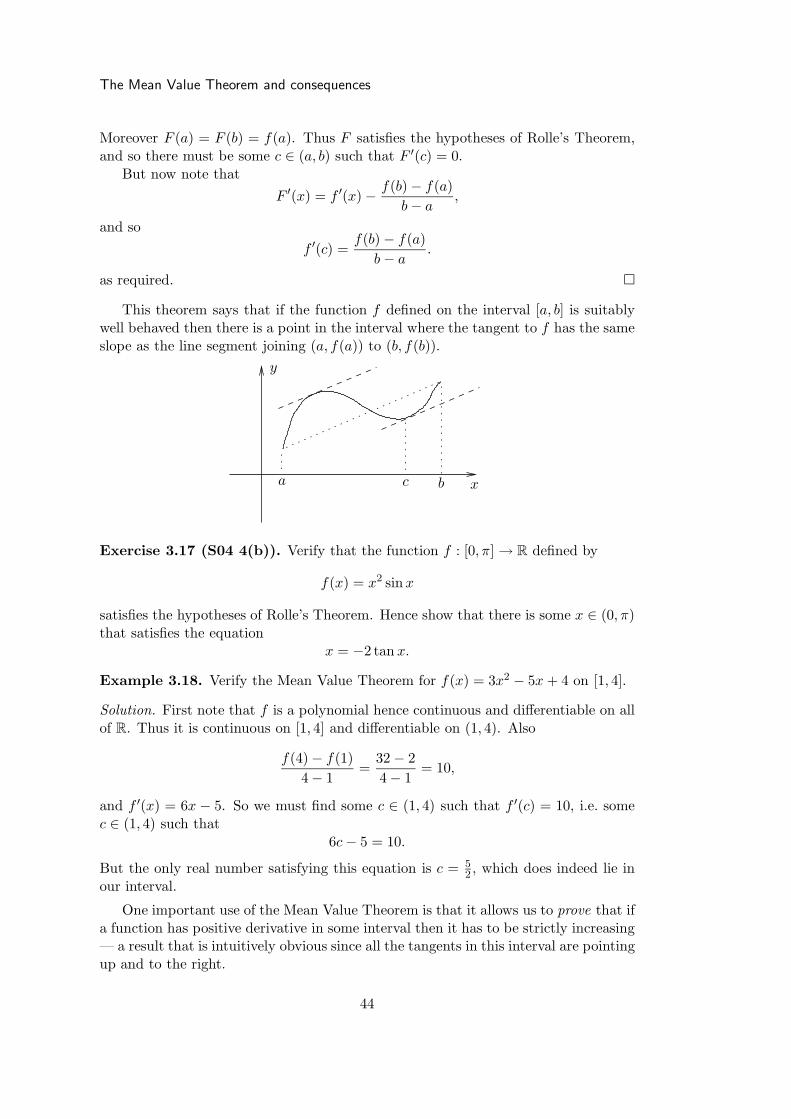
The Mean Value Theorem and consequences
Moreover F (a) = F (b) = f(a). Thus F satisfies the hypotheses of Rolle’s Theorem,and so there must be some c ∈ (a, b) such that F ′(c) = 0.
But now note that
F ′(x) = f ′(x) − f(b) − f(a)
b − a,
and so
f ′(c) =f(b) − f(a)
b − a.
as required.
This theorem says that if the function f defined on the interval [a, b] is suitablywell behaved then there is a point in the interval where the tangent to f has the sameslope as the line segment joining (a, f(a)) to (b, f(b)).
y
xa bc
Exercise 3.17 (S04 4(b)). Verify that the function f : [0, π] → R defined by
f(x) = x2 sin x
satisfies the hypotheses of Rolle’s Theorem. Hence show that there is some x ∈ (0, π)that satisfies the equation
x = −2 tan x.
Example 3.18. Verify the Mean Value Theorem for f(x) = 3x2 − 5x + 4 on [1, 4].
Solution. First note that f is a polynomial hence continuous and differentiable on allof R. Thus it is continuous on [1, 4] and differentiable on (1, 4). Also
f(4) − f(1)
4 − 1=
32 − 2
4 − 1= 10,
and f ′(x) = 6x − 5. So we must find some c ∈ (1, 4) such that f ′(c) = 10, i.e. somec ∈ (1, 4) such that
6c − 5 = 10.
But the only real number satisfying this equation is c = 52 , which does indeed lie in
our interval.
One important use of the Mean Value Theorem is that it allows us to prove that ifa function has positive derivative in some interval then it has to be strictly increasing— a result that is intuitively obvious since all the tangents in this interval are pointingup and to the right.
44

DIFFERENTIATION
Proposition 3.19. Suppose that the function f is differentiable on (a, b) for some
a, b ∈ R such that a < b.
(a) If f ′(x) = 0 for all x ∈ (a, b) then f is constant.
(b) If f ′(x) > 0 for all x ∈ (a, b) then f is strictly increasing.
(c) If f ′(x) < 0 for all x ∈ (a, b) then f is strictly decreasing.
Proof. To show that f is constant if it has zero derivative fix any two points x1, x2 ∈(a, b) with x1 < x2. Then f restricted to [x1, x2] satisfies the hypotheses of the MeanValue Theorem and so there is some c ∈ (x1, x2) such that
f ′(c) =f(x2) − f(x1)
x2 − x1. (†)
But by assumption f ′(c) = 0, hence we must have f(x1)−f(x2) = 0, so that f(x1) =f(x2) as required.
If, instead, f ′(x) > 0 for all x ∈ (a, b), then the same argument produces ac ∈ (x1, x2) such that (†) holds, and now our assumption is that f ′(c) > 0. But thisin turn implies that f(x2) − f(x1) > 0 (since x2 − x1 > 0) and so f(x2) > f(x1) asrequired. The proof of part (c) is similar.
The techniques we have developed so far allow us to prove the existence of nthroots of nonnegative real numbers. In fact our work can extended as follows. For anypositive rational number r (that is any number of the form r = m
n for integers m ≥ 1and n ≥ 1) we can make the following definition
xr = (x1/n)m for all x > 0.
That is, take the nth root of x then raise it to the mth power. Using the uniquenessaspect of Proposition 2.33 we can show that this definition does not depend on theway we write r (for example if we took r = 1
2 , then we also have r = 36 , and so
we should check that x1/2 = (x1/6)3), and also that xr = (xm)1/n. Moreover theuniqueness implies that the following formulae hold:
(xr)s = xrs, xrxs = xr+s
for all x > 0 and positive rationals r and s. Furthermore, if we define x−r to be1
xrand x0 = 1 for all x > 0 then the above formulae remain true for any choice of
rationals r and s.
Similarly we can use aspects of the Mean Value Theorem etc. to actually define
what we mean by log x and ex. Indeed, one way to define the natural logarithm is toset
log x =
∫ x
1
1
tdt for all x > 0.
That is log x is the integral of1
tfrom 1 to x — the theory of integration is covered
in detail in MS2002. Immediate consequences of this definition are that log 1 = 0
45
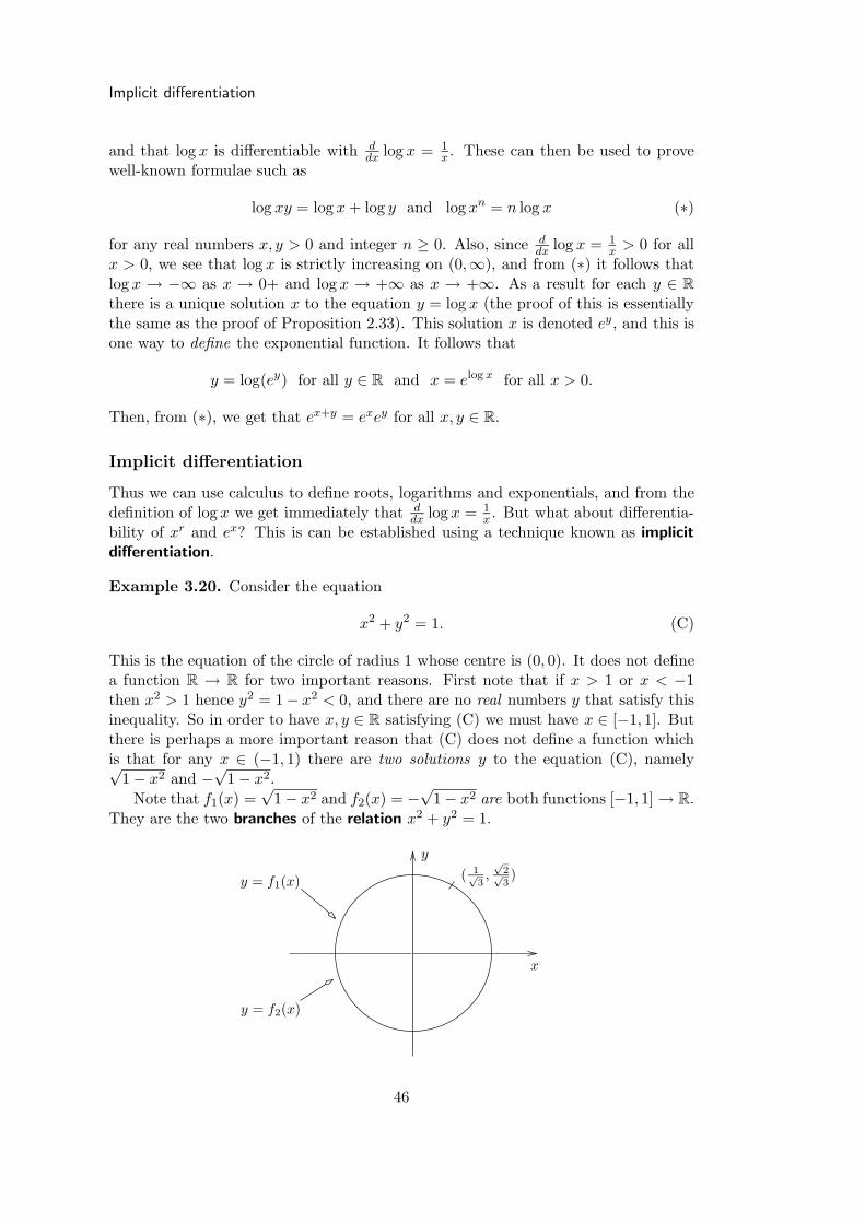
Implicit differentiation
and that log x is differentiable with ddx log x = 1
x . These can then be used to provewell-known formulae such as
log xy = log x + log y and log xn = n log x (∗)
for any real numbers x, y > 0 and integer n ≥ 0. Also, since ddx log x = 1
x > 0 for allx > 0, we see that log x is strictly increasing on (0,∞), and from (∗) it follows thatlog x → −∞ as x → 0+ and log x → +∞ as x → +∞. As a result for each y ∈ R
there is a unique solution x to the equation y = log x (the proof of this is essentiallythe same as the proof of Proposition 2.33). This solution x is denoted ey, and this isone way to define the exponential function. It follows that
y = log(ey) for all y ∈ R and x = elog x for all x > 0.
Then, from (∗), we get that ex+y = exey for all x, y ∈ R.
Implicit differentiation
Thus we can use calculus to define roots, logarithms and exponentials, and from thedefinition of log x we get immediately that d
dx log x = 1x . But what about differentia-
bility of xr and ex? This is can be established using a technique known as implicit
differentiation.
Example 3.20. Consider the equation
x2 + y2 = 1. (C)
This is the equation of the circle of radius 1 whose centre is (0, 0). It does not definea function R → R for two important reasons. First note that if x > 1 or x < −1then x2 > 1 hence y2 = 1− x2 < 0, and there are no real numbers y that satisfy thisinequality. So in order to have x, y ∈ R satisfying (C) we must have x ∈ [−1, 1]. Butthere is perhaps a more important reason that (C) does not define a function whichis that for any x ∈ (−1, 1) there are two solutions y to the equation (C), namely√
1 − x2 and −√
1 − x2.
Note that f1(x) =√
1 − x2 and f2(x) = −√
1 − x2 are both functions [−1, 1] → R.They are the two branches of the relation x2 + y2 = 1.
y
y = f1(x)
y = f2(x)
x
( 1√3,√
2√3)
46
DIFFERENTIATION
Suppose we wanted to find the equation of the tangent to the point ( 1√3,√
2√3)
on (C). This lies on the branch f1, and so we could calculate f ′1(
1√3) to find the slope
of the tangent.However, an alternative is to instead differentiate the equation (C) directly. We
think of y as a function of x, then y2 is the product of y with itself and so the productrule tells us that
d
dx(y2) =
dy
dx× y + y × dy
dx= 2y
dy
dx.
So then differentiating (C) gives
d
dx(x2 + y2) =
d
dx(1) ⇒ 2x + 2y
dy
dx= 0 ⇒ dy
dx= −2x
2y= −x
yif y 6= 0.
Thus when x = 1√3
and y =√
2√3
we have
dy
dx= −
1√3√2√3
= − 1√2,
and so the tangent is
y −√
2√3
= − 1√2(x − 1√
3) ⇔
√2y + x =
√3.
If we wanted to use the more traditional route then we would have to differentiatef1(x) =
√1 − x2. We know how to differentiate the function f(x) = 1−x2 inside the
square root (f ′(x) = −2x for all x ∈ R), and so if we wanted to apply the chain ruleto find f ′
1(x) then we need to know how to differentiate square roots. The followinganswers this problem:
Proposition 3.21. For any rational number r the function f(x) = xr is differentiable
on (0,∞) with f ′(x) = rxr−1 (cf. the case when r is an integer).
Proof. Suppose we have r = mn for integers m and n, and let y = xr = (xm)1/n.
Raising both sides to the nth power gives
yn =((xm)1/n
)n= (xm)1 = xm.
Thus we can differentiate both sides, using the chain rule on the left hand side, to get
nyn−1 × dy
dx= mxm−1
Since y > 0 we can divide both sides by yn−1 to get
dy
dx=
mxm−1
nyn−1=
m
n× xm−1
((x1/n)m
)n−1 = rxm−1−m(n−1)n
and
m − 1 − m(n − 1)
n=
n(m − 1) − m(n − 1)
n=
m − n
n= r − 1
as required.
47
Implicit differentiation
Recall that for each x ∈ R the number ex is the unique solution y to the equationx = log y. Differentiating this equation with respect to x and noting that d
dt log t = 1t
we can arrive at the formula ddxex = ex in a similar way to the proposition above.
Indeed, using exponentials and logarithms we can actually define xr for any x > 0and all r ∈ R, and establish the formula d
dxxr = rxr−1 by an alternative route thatinvolves the chain rule.
Exercise 3.22 (A03 6(a)). Find the tangent to the implicitly defined curve
x sin y + cos x + e− sinx = e−1
at the point (π2 , π). Where does this tangent intersect the x-axis?
48

CURVE SKETCHING AND MINMAX PROBLEMS
4 Curve Sketching and MinMax Problems
Maxima and minima
Definition 4.1. Let f : R → R be a function and a, b ∈ R. Then f has a local
maximum at a if there is some interval (c1, d1) ⊂ R such that a ∈ (c1, d1) and
f(x) ≤ f(a) for all x ∈ (c1, d1).
Similarly, f has a local minimum at b if there is some interval (c2, d2) ⊂ R such thatb ∈ (c2, d2) and
f(x) ≥ f(b) for all x ∈ (c2, d2).
Note that we do not require that f(a) be the largest value that the function evertakes, only that it is greater than f(x) for all x (sufficiently) close to a. Similarly forf(b). Consider the following graph of a function f defined on an interval [a, e]:
y
xa b c de
Here b is the absolute maximum (and also a local maximum), a and c are localminima, d a local maximum and e the absolute minimum.
The next result gives a method for locating local maxima and minima.
Proposition 4.2. Let f be a continuous function on the interval [c, d]. If f attains its
maximum value at some x1 ∈ (c, d) and is differentiable at this point, then f ′(x1) = 0.Similarly if f attains its minimum value at some x2 ∈ (c, d) and is differentiable there,
then f ′(x2) = 0.
Proof. This is essentially a rehash of the proof of Rolle’s Theorem. Since f(x1) is themaximum value that f takes on this interval, f(x1 + h) ≤ f(x1) for all h 6= 0, so that
f(x1 + h) − f(x1) ≤ 0 for all h 6= 0.
But f is differentiable at x1 so the left and right derivatives must exist, and theymust be equal to f ′(x1). Hence
f(x1 + h) − f(x1)
h≥ 0 for all h < 0
and so
f ′(x1) = f ′−(x1) = lim
h→0−f(x1 + h) − f(x1)
h≥ 0.
Similarly
f ′(x1) = f ′+(x1) = lim
h→0+
f(x1 + h) − f(x1)
h≤ 0,
49

The second derivative test
since now we require h > 0 in the limit. Thus we must have f ′(x1) = 0, as required.The proof for the point x2 runs along the same lines.
So to look for the local maxima and minima of a differentiable function f weshould calculate its derivative f ′ and look for solutions of the equation f ′(x) = 0,since if f has a local maximum or minimum at some point a then clearly we canrestrict f to an interval of the form [c, d] such that a ∈ (c, d) and f(a) is the absolutemaximum or minimum for this restriction. The points where f ′(x) = 0 are known ascritical or stationary points of the function f .
Exercise 4.3. Examine the critical points of the function f : [−3, 3] → R defined byf(x) = x3 − 3x and sketch its graph.
The second derivative test
In the previous example it was easy to determine which critical point was a localmaximum and which a local minimum since the function was relatively simple. Thismay not always be the case and so we now develop a more methodical techniquefor analysing this question. Suppose f : R → R is a function that is differentiableeverywhere on R, then we have a new function f ′ : R → R defined by setting
f ′(x) = limh→0
f(x + h) − f(x)
h
for each x ∈ R. The number f ′(x) is a measure of the rate at which the function ischanging at the point x — it is the slope of the tangent to the graph of f at thispoint. If it is positive then f is increasing and if it is negative then f is decreasing.Moreover if f has a local maximum or minimum at x then f ′(x) = 0.
So now suppose that the function f ′ is itself differentiable. That is for each x thefollowing limit exists:
limh→0
f ′(x + h) − f ′(x)
h.
The resulting function is called the second derivative of f and is denoted f ′′, that is,f ′′ = (f ′)′. If we are writing y = f(x) then the derivative and second derivative are
often denoted dydx and d2y
dx2 respectively.
Suppose f and f ′ are differentiable (with f ′′ continuous) and that f ′(a) = 0 andf ′′(a) > 0 for some a ∈ R. Then the function f ′(x) is increasing at x = a, that is thegradient of f at x = a is increasing. Since it is zero at x = a it must be negative tothe immediate left of a and positive to the immediate right. That is, the graph musttake the form
horizonal tangent
positive slopenegative slope
50
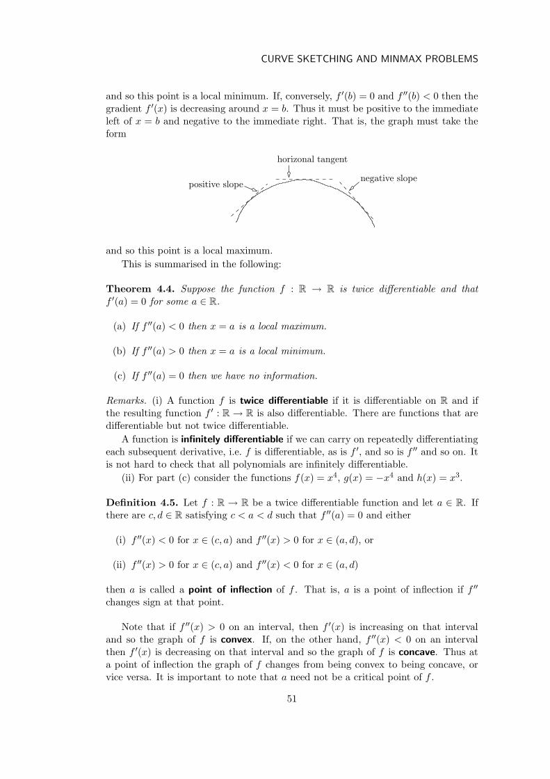
CURVE SKETCHING AND MINMAX PROBLEMS
and so this point is a local minimum. If, conversely, f ′(b) = 0 and f ′′(b) < 0 then thegradient f ′(x) is decreasing around x = b. Thus it must be positive to the immediateleft of x = b and negative to the immediate right. That is, the graph must take theform
PSfrag
horizonal tangent
positive slopenegative slope
and so this point is a local maximum.
This is summarised in the following:
Theorem 4.4. Suppose the function f : R → R is twice differentiable and that
f ′(a) = 0 for some a ∈ R.
(a) If f ′′(a) < 0 then x = a is a local maximum.
(b) If f ′′(a) > 0 then x = a is a local minimum.
(c) If f ′′(a) = 0 then we have no information.
Remarks. (i) A function f is twice differentiable if it is differentiable on R and ifthe resulting function f ′ : R → R is also differentiable. There are functions that aredifferentiable but not twice differentiable.
A function is infinitely differentiable if we can carry on repeatedly differentiatingeach subsequent derivative, i.e. f is differentiable, as is f ′, and so is f ′′ and so on. Itis not hard to check that all polynomials are infinitely differentiable.
(ii) For part (c) consider the functions f(x) = x4, g(x) = −x4 and h(x) = x3.
Definition 4.5. Let f : R → R be a twice differentiable function and let a ∈ R. Ifthere are c, d ∈ R satisfying c < a < d such that f ′′(a) = 0 and either
(i) f ′′(x) < 0 for x ∈ (c, a) and f ′′(x) > 0 for x ∈ (a, d), or
(ii) f ′′(x) > 0 for x ∈ (c, a) and f ′′(x) < 0 for x ∈ (a, d)
then a is called a point of inflection of f . That is, a is a point of inflection if f ′′
changes sign at that point.
Note that if f ′′(x) > 0 on an interval, then f ′(x) is increasing on that intervaland so the graph of f is convex. If, on the other hand, f ′′(x) < 0 on an intervalthen f ′(x) is decreasing on that interval and so the graph of f is concave. Thus ata point of inflection the graph of f changes from being convex to being concave, orvice versa. It is important to note that a need not be a critical point of f .
51
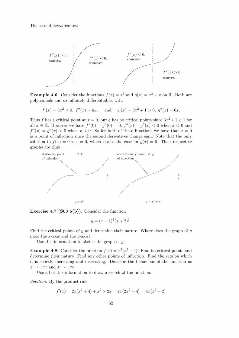
The second derivative test
f ′′(x) < 0,f ′′(x) < 0,
f ′′(x) > 0,
f ′′(x) > 0,
convex
convex
concaveconcave
Example 4.6. Consider the functions f(x) = x3 and g(x) = x3 + x on R. Both arepolynomials and so infinitely differentiable, with
f ′(x) = 3x2 ≥ 0, f ′′(x) = 6x, and g′(x) = 3x2 + 1 > 0, g′′(x) = 6x.
Thus f has a critical point at x = 0, but g has no critical points since 3x2 + 1 ≥ 1 forall x ∈ R. However we have f ′′(0) = g′′(0) = 0, f ′′(x) = g′′(x) < 0 when x < 0 andf ′′(x) = g′′(x) > 0 when x > 0. So for both of these functions we have that x = 0is a point of inflection since the second derivatives change sign. Note that the onlysolution to f(x) = 0 is x = 0, which is also the case for g(x) = 0. Their respectivegraphs are thus
yy
y = x3 y = x3 + x
stationary point nonstationary point
of inflectionof inflection
xx
Exercise 4.7 (S03 5(b)). Consider the function
y = (x − 1)2(x + 2)2.
Find the critical points of y and determine their nature. Where does the graph of ymeet the x-axis and the y-axis?
Use this information to sketch the graph of y.
Example 4.8. Consider the function f(x) = x2(x2 + 4). Find its critical points anddetermine their nature. Find any other points of inflection. Find the sets on whichit is strictly increasing and decreasing. Describe the behaviour of the function asx → +∞ and x → −∞
Use all of this information to draw a sketch of the function.
Solution. By the product rule
f ′(x) = 2x(x2 + 4) + x2 × 2x = 2x(2x2 + 4) = 4x(x2 + 2)
52

CURVE SKETCHING AND MINMAX PROBLEMS
which is equal to zero precisely when x = 0 since x2 + 2 ≥ 2 for all x ∈ R. Also,
f ′′(x) = 4(x2 + 2) + 4x × 2x = 12x2 + 8
which is greater than zero for all x. In particular f ′′(0) = 8 > 0, and so thereis a minimum when x = 0 and f(0) = 0. Also, there are no points of inflection.Moreover, because x2 + 2 > 0 for all x ∈ R, f is strictly increasing on (0,∞) andstrictly decreasing on (−∞, 0).
Since f(x) = x4(1 + 4x2 ), we have that f(x) ≈ x4 for large x, since 4
x2 → 0 asx → ±∞. Thus f(x) → +∞ as x → +∞ and as x → −∞. Hence the graph of f isof the form:
x
y
0
Exercise 4.9 (S02 5(b)). For the function
g(x) =2x
3x2 + 1
find the critical points and their nature, find the sets on which g is strictly increasingand strictly decreasing, and find the points of inflection. What happens as x → +∞and x → −∞?
Use this information to sketch the graph of g.
Example 4.10. Consider the function f(x) = (x − 1)5. Find its critical points anddetermine their nature. Find any other points of inflection. Find the sets on whichit is strictly increasing and decreasing. Describe the behaviour of the function asx → +∞ and x → −∞
Use all of this information to draw a sketch of the function.
Solution. Applying the chain rule twice we get
f ′(x) = 5(x − 1)4 and f ′′(x) = 20(x − 1)3.
Thus f ′(x) = 0 precisely when x = 1, and f ′′ changes sign at this point. For all otherx we have that f ′(x) > 0, so that f is strictly increasing on (−∞, 1) and (1,∞),and there is one critical point, but it is a point of inflection rather than being alocal maximum or minimum. Note that f(x) = 0 exactly when x = 1. Finally, wehave f(x) = [x(1 − 1
x)]5 = x5(1 − 1x)5, and since 1
x → 0 as x → ±∞, we have that(1 − 1
x)5 → 1, and so f(x) ≈ x5 for large x. Thus f(x) → +∞ as x → +∞ andf(x) → −∞ as x → −∞. Hence the graph of f is of the form:
53
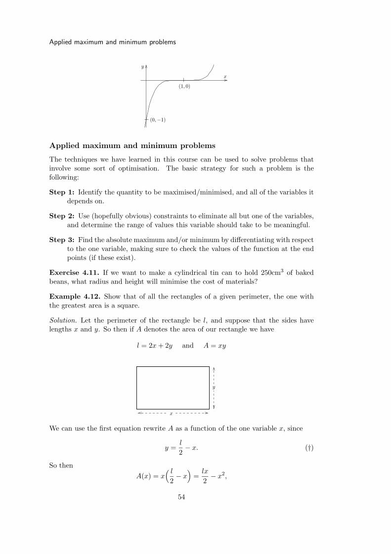
Applied maximum and minimum problems
x
y
(0,−1)
(1, 0)
Applied maximum and minimum problems
The techniques we have learned in this course can be used to solve problems thatinvolve some sort of optimisation. The basic strategy for such a problem is thefollowing:
Step 1: Identify the quantity to be maximised/minimised, and all of the variables itdepends on.
Step 2: Use (hopefully obvious) constraints to eliminate all but one of the variables,and determine the range of values this variable should take to be meaningful.
Step 3: Find the absolute maximum and/or minimum by differentiating with respectto the one variable, making sure to check the values of the function at the endpoints (if these exist).
Exercise 4.11. If we want to make a cylindrical tin can to hold 250cm3 of bakedbeans, what radius and height will minimise the cost of materials?
Example 4.12. Show that of all the rectangles of a given perimeter, the one withthe greatest area is a square.
Solution. Let the perimeter of the rectangle be l, and suppose that the sides havelengths x and y. So then if A denotes the area of our rectangle we have
l = 2x + 2y and A = xy
x
y
We can use the first equation rewrite A as a function of the one variable x, since
y =l
2− x. (†)
So then
A(x) = x( l
2− x
)=
lx
2− x2,
54

CURVE SKETCHING AND MINMAX PROBLEMS
and we must have 0 ≤ x ≤ l/2 to ensure that the lengths x and y are both nonnegative.Differentiating with respect to x gives
A′(x) =l
2− 2x
which is equal to 0 when x = l/4. That is, there is a stationary point when x = l/4.But since A(0) = 0, A(l/4) = l2/8− l2/16 = l2/8 > 0 and A(l/2) = 0 we see that themaximum area occurs when x = l/4. When this happens we have from (†) that
y =l
2− l
4=
l
4= x
and so our rectangle is in fact a square as required.
Exercise 4.13. A woman at a point A on the shore of a circular lake with radius2km wants to arrive at the point C diametrically opposite A on the other side of thelake in the shortest possible time. She can walk at the rate of 4km/h, and row a boatat 2km/h. How should she proceed?
Example 4.14. A box with an open top is to be constructed from a square piece ofcardboard 4m wide by cutting out a square from each of the four corners and bendingup the sides. Find the largest volume such a box can have.
Solution. The diagram for this situation is:
x
x4 − 2x
4 − 2x
4 − 2x
4
where x is the length of the side of the square removed from each corner. Since thetotal length is 4m, the length of a side of the base is 4 − 2 × x = 2(2 − x)m. Thusthe area of the base will be [2(2 − x)]2 = 4(2 − x)2 m2. Moreover, the height of thebox will be xm, and so the overall volume is
V (x) = x × 4(2 − x)2 = 4x(2 − x)2
and note that we must have x ≥ 0, and 4 − 2x ≥ 0, so that we must only considerx ∈ [0, 2]. But differentiating with respect to x gives
V ′(x) = 4 × (2 − x)2 + 4x × 2(2 − x) × (−1) = 4(2 − x)[(2 − x) − 2x
]
= 4(2 − x)(2 − 3x)
which is zero precisely when x = 2 and x = 23 . The maximum value of V will occur at
either one of these values, or when x = 0, which is the other endpoint for the intervalof values x may assume. But
V (0) = V (2) = 0, and V(2
3
)= 4 × 2
3×
(4
3
)2=
128
27.
Thus the largest volume is 32m3.
55

Applied maximum and minimum problems
Exercise 4.15 (S02 6(b)). A Norman window has the shape of a rectangle sur-mounted by a semicircle (Thus the diameter of the semicircle is equal to the widthof the rectangle). If the perimeter of the window is 10m, find the dimensions of thewindow so that the greatest possible amount of light is admitted.
What is the area of the window when this achieved?
Example 4.16. Find the point on the parabola y = x2 that is closest to the point(3, 0).
Solution. Consider the following diagram representing this situation:
x
y
(x, x2)
y = x2
(3, 0)
If d denotes the distance of the point (3, 0) from a general point on the parabola(x, x2) then we have
d(x) =√
(x − 3)2 + (x2 − 0)2
by Pythagoras’ Theorem. We wish to minimise the value of d as x varies, but theminimum value of d will occur for the same value of x as the minimum value of thefunction D = d2, and it is easier to minimise D since it does not involve square roots.So we have
D(x) = (x − 3)2 + x4 = x4 + x2 − 6x + 9
and henceD′(x) = 4x3 + 2x − 6 = 2(2x3 + x − 3).
By inspection we see that x = 1 is a root of D′(x) = 0, and in fact
D′(x) = 2(x − 1)(2x2 + 2x + 3).
But 2x2 + 2x + 3 = 2(x + 12)2 + 5
2 > 0 for all x, and so D′(x) = 0 only when x = 1.Also,
D′′(x) = 12x2 + 2 > 0
for all x, so that we have a local minimum when x = 1. Thus the point on y = x2
that is closest to (3, 0) is when x = 1 and so y = 12 = 1 as well. Thus the requiredpoint is (1, 1).
Exercise 4.17. Find the area of the largest rectangle that can be inscribed in asemicircle of radius r, with one side of the rectangle on the straight side of thesemicircle.
Example 4.18. Find the equation of the line through the point (3, 5) that cuts offthe least area from the first quadrant.
56
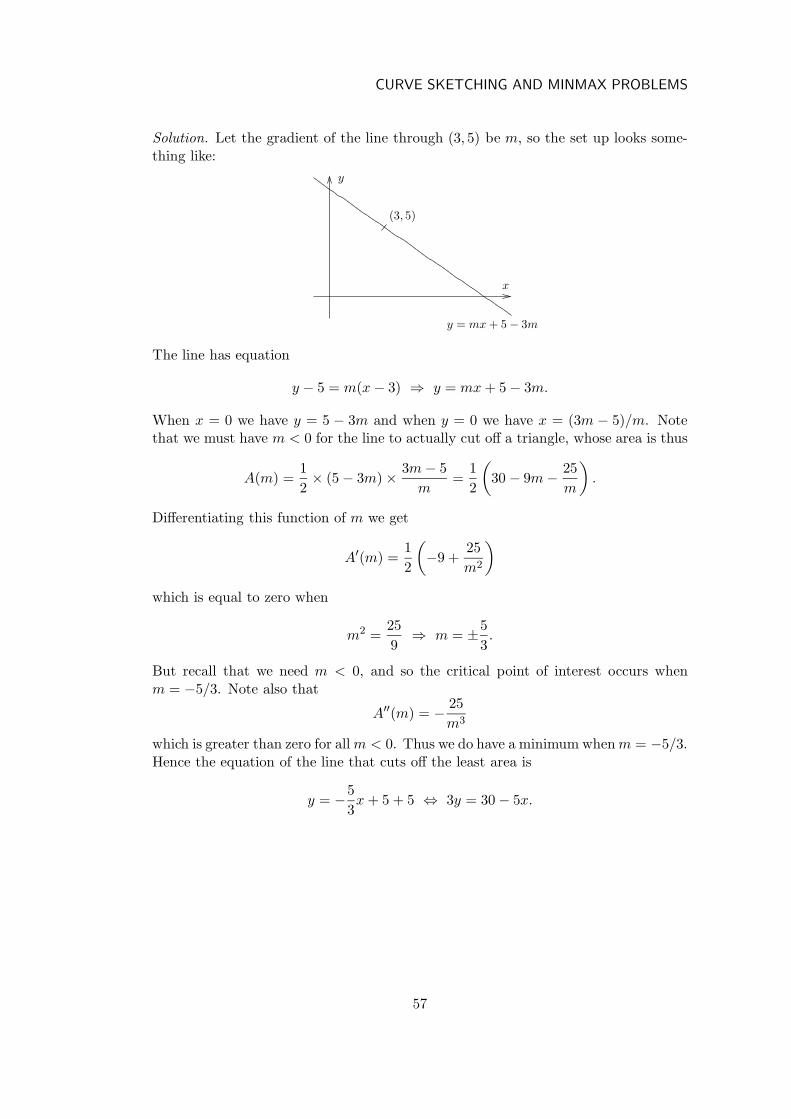
CURVE SKETCHING AND MINMAX PROBLEMS
Solution. Let the gradient of the line through (3, 5) be m, so the set up looks some-thing like:
x
y
(3, 5)
y = mx + 5 − 3m
The line has equation
y − 5 = m(x − 3) ⇒ y = mx + 5 − 3m.
When x = 0 we have y = 5 − 3m and when y = 0 we have x = (3m − 5)/m. Notethat we must have m < 0 for the line to actually cut off a triangle, whose area is thus
A(m) =1
2× (5 − 3m) × 3m − 5
m=
1
2
(30 − 9m − 25
m
).
Differentiating this function of m we get
A′(m) =1
2
(−9 +
25
m2
)
which is equal to zero when
m2 =25
9⇒ m = ±5
3.
But recall that we need m < 0, and so the critical point of interest occurs whenm = −5/3. Note also that
A′′(m) = − 25
m3
which is greater than zero for all m < 0. Thus we do have a minimum when m = −5/3.Hence the equation of the line that cuts off the least area is
y = −5
3x + 5 + 5 ⇔ 3y = 30 − 5x.
57