United States Department of Agriculture

Forest Service

Intermountain Research Station

Research Paper INT-414

November 1989

MTCLIM: A Mountain Microclimate Simulation Model Roger D. Hungerford Ramakrishna R. Nemani Steven W. Running Joseph C. Coughlan

This file was created by scanning the printed publication.Errors identified by the software have been corrected;

however, some errors may remain.

THE AUTHORS

ROGER D. HUNGERFORD is a research forester at the Intermountain Fire Sciences Laboratory in Missoula, MT. His current research includes forest micrometeorology and fire effects studies.

RAMAKRISHNA R. NEMANI is a research assistant in the School of Forestry, University of Montana, Missoula, MT. He is currently using satellite imagery to estimate forest productivity.

STEVEN W. RUNNING is a professor in the School of For­estry, University of Montana. He is conducting research on plant-water relations, tree physiology, and remote sensing techniques for estimating site productivity.

JOSEPH C. COUGHLAN is a research assistant in the School of Forestry, University of Montana. He is currently working on expert systems to efficiently apply ecosystem models in a Geographic Information System.

RESEARCH SUMMARY

The MTCLIM model predicts daily solar radiation, air tem­perature, relative humidity, and precipitation for mountainous sites by extrapolating data measured at National Weather Service stations. The model may be used to generate data for use in fire models, ecological models, insect and disease models, or developing silvicultural prescriptions. Potential applications are discussed in this paper.

This paper gives the rationale for the MTCLIM model and describes how to execute the model. Preparation of input, adjustment of coefficients, and interpretation of output are discussed. MTCLIM is available on the Forest Service's Data General System and on IBM and IBM-compatible systems.

Evaluation of model outputs (solar radiation, air tempera­ture, relative humidity, and precipitation) are presented by comparing MTCLIM-predicted data with observed data. These tests were run using observed data from up to nine different sites not used in developing the model. Results of these evaluations show that MTCLIM predicts daylight aver­age and maximum air temperatures with an accuracy of 4 °F (f >0.86) and minimum temperatures with an accuracy of 6 oF (f >0.56). Predictions of solar radiation are accurate to 100 W/m2 (f >0.50) and relative humidity to 11 percent (f >0.43). Precipitation predictions are accurate within 0.15 inches (f >0.49) when two base stations are used. Adjust­ments to coefficients are discussed relative to these evalu­ations and how the values might be changed to reflect different conditions from the Northern Rocky Mountains where MTCLIM was developed.

CONTENTS

Introduction .................................................................... ~~~~ Description of MTCLIM ........................................................ 1

Base Station Inputs .......................................................... 1 Model Components ........................................................ 2 Definition of Variables ...................................................... 2 Time Scales of Prediction ................................................ 2 Units of Measurement. ..................................................... 2 Description of Subroutines ............................................... 2

Executing MTCLIM .............................................................. 6 Location of the Program ................................................... 6 Creating Input Files .......................................................... 6 MTCLIM Output File ....................................................... 11 Executing MTCLIM ......................................................... 14

Evaluation of MTCLIM ....................................................... 14 Procedures ..................................................................... 14 Solar Radiation ............................................................... 14 Temperature .................................................................. 17 Humidity ......................................................................... 22 Precipitation ................................................................... 23

Using MTCLIM as a Management Tool ............................. 25 Ecosystem Modeling Applications .................................. 25 Silviculture ...................................................................... 25 Fire ................................................................................. 26 Hydrology ....................................................................... 26 Insects and Disease ....................................................... 27

References ........................................................................ 27 Appendix A: Listing of MTCLIM Program in

FORTRAN Code .............................................................. 31 Appendix B: Sine Form for Averaging Temperature ......... .46 Appendix C: Estimating Daily Dewpoint Temperature ....... 47 Appendix D: Equations for Calculating Solar Radiation .... 48 Appendix E: Calculating Horizon Angles From a Topographic Map ............................................................. 50

Appendix F: Equations for Calculating Precipitation .......... 51 Appendix G: Equations for Calculating Humidity ............... 52

The use and trade of firm names in this publication is for reader information and does not imply endorsement by the U.S. Department of any product or service.

Intermountain Research Station 324 25th Street

Ogden, UT 84401

Base Station Inputs

MTCLIM: A Mountain Microclimate Simulation Model Roger D. Hungerford Ramakrishna R. Nemani Steven W. Running Joseph C. Coughlan

INTRODUCTION

This paper presents the logic and equations of a mountain microclimate simula­tor (MTCLIM) that is designed to extrapolate routine National Weather Service (NWS) data to adjacent mountainous terrain. Typically, meteorological data are measured at city airports in valley bottoms and are not available for mountainous terrain.

Other papers (Running and Hungerford 1983; Running and others 1987) have reported on initial tests of extrapolation and the use of MTCLIM for ecological mod­eling. Originally the model was designed to interface with ecological models, but we have restructured some parts to make it useful for other purposes. This paper pres­ents the modifications and results of further testing by comparing model outputs with observed data. We also describe how to use the model, including some specific applications.

The paper is divided into the following sections:

1. Description of MTCLIM and the model components. 2. Executing MTCLIM, including a description of inputs and outputs tailored for

Data General and IBM-PC systems. 3. Evaluation of the model outputs using predicted vs. observed regression

analysis. 4. Applying MTCLIM as a management tool.

DESCRIPTION OF MTCLIM

The mountain microclimate simulator (MTCLIM) extrapolates meteorological variables from a point of measurement (referred to as the "base" station) to the study "site" of interest, making corrections for differences in elevation, slope, and aspect between the base station and the site. The first step in using MTCLIM is to determine the appropriate synoptic meteorological database. The Forest Service, U.S. Department of Agriculture, National Fire Danger Rating System (NFDRS) (Furman and Brink 1975) has an extensive network of stations throughout the for­ested region of the Western United States, but operates only during the summer fire months. Remote Automated Weather Stations (RAWS) are being established in mountainous areas throughout the West, but the data are not routinely available to users outside the Federal agencies (Warren and Vance 1981), and many operate only during the summer months. Another source, and the one we used in develop­ing MTCLIM, is the Climatological Data summary compiled by the National Oceanic and Atmospheric Administration (NOAA), National Climatic Center, Asheville, NC. These stations, operated by the National Weather Service (NWS), are usually located at major airports.

Data for NWS stations are compiled monthly for each State, giving daily air tem­perature and precipitation at secondary stations; and dewpoint, cloud cover, sun­shine duration, windspeed, and other variables at major airport stations. MTCLIM uses vertical (elevation-related) corrections to extrapolate from NWS stations to

Model Components

Definition of Variables

Time Scales of Prediction

Units of Measurement

Description of Subroutines

adjacent mountainous sites. Accuracy of extrapolation decreases as distance (hori­zontal) between a base station and study site increases, because of changes in air masses, cloud cover, and precipitation. Selection of representative base stations is discussed in the section describing creation of input files.

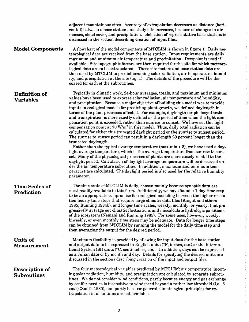
A flowchart of the model components ofMTCLIM is shown in figure 1. Daily me­teorological data are received from the base station. Input requirements are daily maximum and minimum air temperature and precipitation. Dewpoint is used if available. Site topographic factors are then required for the site for which meteoro­logical data are to be extrapolated. These site factors and base station data are then used by MTCLIM to predict incoming solar radiation, air temperature, humid­ity, and precipitation at the site (fig. 1). The details of the procedure will be dis­cussed for each of the subroutines.

Typically in climatic work, 24-hour averages, totals, and maximum and minimum values have been used to express solar radiation, air temperature and humidity, and precipitation. Because a major objective of building this model was to provide inputs to ecological models for predicting plant growth, we defined daylength in terms of the plant processes affected. For example, day length for photosynthesis and transpiration is more exactly defined as the period of time when the light com­pensation point is exceeded, rather than sunrise to sunset. We have set this light compensation point at 70 W/m2 in this model. Thus, daily total radiation can be calculated for either this truncated daylight period or the sunrise to sunset period. The sunrise to sunset period can result in a day length 20 percent longer than the truncated daylength.

Rather than the typical average temperature (max-min + 2), we have used a day­light average temperature, which is the average temperature from sunrise to sun­set. Many of the physiological processes of plants are more closely related to the daylight period. Calculation of daylight average temperature will be discussed un­der the air temperature subroutine. In addition, maximum and minimum tem­perature are calculated. The daylight period is also used for the relative humidity parameter.

The time scale ofMTCLIM is daily, chosen mainly because synoptic data are most readily available in this form. Additionally, we have found a 1-day time step to be an appropriate compromise for ecological modeling between the higher resolu­tion hourly time steps that require large climatic data files (Knight and others 1985; Running 1984b), and longer time scales, weekly, monthly, or yearly, that pro­gressively average out climatic fluctuations and miscalculate hydrologic partitions of the ecosystem (Nemani and Running 1985). For some uses, however, weekly, biweekly, or even monthly time steps may be adequate. Data for longer time steps can be obtained from MTCLIM by running the model for the daily time step and then averaging the output for the desired period.

Maximum flexibility is provided by allowing for input data for the base station and output data to be expressed in English units (°F, inches, etc.) or the Interna­tional System (SI) units (°C, centimeters, etc.). In addition, days can be expressed as a Julian date or by month and day. Details for specifying the desired units are discussed in the sections describing creation of the input and output files.

The four meteorological variables predicted by MTCLIM: air temperature, incom­ing solar radiation, humidity, and precipitation are calculated by separate subrou­tines. We do not consider wind conditions, partly because energy and gas exchange by conifer needles is insensitive to windspeed beyond a rather low threshold (i.e., 5 cm/s) (Smith 1980), and partly because general climatological principles for ex­trapolation in mountains are not available.

2

MTCLIM

MOUNTAIN MICROCLIMATE MODEL

SITE FACTORS ELEVATION, SLOPE, ASPECT, E-W HORIZON ANGLES, STAND LAI OR BASAL AREA, BASE STATION IDENTITY

BASE STATION AIR TEMPERATURE, (MAX-MIN, DAILY), DEWPOINT (24-H AV), PRECIPITATION (DAILY)

SUBROUTINES

I SOLAR RADIATION I CALCULATE DAY LENGTH

+ POTENTIAL RADIATION

(SLOPE, ASPECT, E-W HORIZON CORRECTED)

+ ATMOSPHERIC

TRANSMISSIVITY

+ PSN THRESHOLD

~ INCOMING SHORTWAVE

RADIATION

lAIR TEMPERATURE'

DAYLIGHT AVERAGE FROM MAX-MIN TEMP

+ ELEVATION CORRECTION

~ SLOPE-ASPECT CORRECTION

BASED ON NET SHORTWAVE RADIATION

+ SURFACE ATTENUATION

BASED ON LAI

~ SITE AIR TEMP

HUMIDITY

DAILY DEWPOINT OR NIGHT MIN TEMP

+ ELEVATION CORRECTION

~ SATURATION VAPOR

PRESSURE

SITE HUMIDITY & VPD

Figure 1-Fiowchart of the MTCLIM model for estimating daily microclimate conditions in mountainous terrain. The site factors and base station variables shown are required inputs for the model.

3

PRECIPITATION

ANNUAL PPT FROM ISOHYETMAP

+ SITE/BASE MULTIPLIER

~ DAILY BASE PPT

Solar Radiation-Estimating daily incoming solar radiation proved to be diffi­cult because most NWS stations in Montana do not directly measure incoming radiant energy. NWS data collected are from semiquantitative "sunshine recorders" or qualitatively from observers' cloud cover estimates. After attempting to work with these data to estimate incoming solar radiation (Running and Hungerford 1983; Satterlund and Means 1978), we decided to use the algorithm of Bristow and Campbell (1984) that relates diurnal air temperature amplitude to at­mospheric transmittance. Their analysis requires only daily maximum and mini­mum air temperatures and precipitation. This algorithm (see appendix D) appears to be accurate, having been tested on three sites ranging from maritime to conti­nental climates and accounting for 70 to 90 percent of the variability in daily in­coming radiation on these sites. We first compute clear sky transmissivity for the elevation of the site of interest, assuming clear sky transmittance at mean sea level is 0.65, and increasing 0.008/m of elevation. Final atmospheric transmissivity is then calculated as an exponential function of diurnal temperature amplitude of the base station (Bristow and Campbell 1984). This procedure accounts for clouds, wa­ter vapor, pollutants, and other atmospheric factors that reduce clear sky transmissivity.

Next, a potential radiation model derived from the logic of Garnier and Ohmura (1968), Buffo and others (1972), and Swift (1976) is used to calculate direct and dif­fuse solar radiation. This model accounts for site differences in latitude, slope, and aspect, and it truncates the direct beam solar irradiance by east and west horizons, rather than assuming a flat horizon. Potential above-atmosphere radiation is re­duced by calculated atmospheric transmissivity to produce a final estimate of in­coming solar radiation for the site. The potential radiation model is also run for an equivalent flat surface at the site elevation to generate a ratio of flat surface to slope radiation absorbed. This ratio is used for adjusting air temperature esti­mates at the site. Finally, the daylength is computed by the radiation submodel for each day. Daylength is computed either for sunrise to sunset or for the period that incoming solar radiation exceeds a threshold of 70 W/m2• This is a threshold for conifer stomatal opening, transpiration, and positive net photosynthesis (PSN) used to describe the operational environment of trees (Jarvis and Leverenz 1983). This threshold number can be easily changed for different types of vegetation and produces an operational day length approximately 85 percent of sunrise to sunset. If this threshold is not invoked, total sunrise to sunset solar radiation is computed. Details of the transmissivity and radiation subroutines are shown in appendix D and the MTCLIM code (appendix A).

Air Temperature-Daylight average air temperature is estimated by assuming the diurnal temperature trace to be a sine form, with the maximum and minimum points given by data from the base station. Integrating the sine function over three quadrants (Parton and Logan 1981) yields the following equation for daylight weighted average air temperature:

T = TEMCF * (T - T ) + T ave max mean mean (1)

where:

T = weighted average daylight air temperature ave T = arithmetic mean (T + T . ) + 2 for a day mean max m1n

TEMCF = coefficient to adjust daylight average temperature.

Details of the sine form assumption are shown in appendix B. Daylight average air temperature is then corrected for elevation using a general

lapse rate of 3.5 °F/1,000 ft for summer, reduced by 10 percent on clear days, and increased by 10 percent on cloudy days (Finklin 1983). This lapse rate is close to published values (3.0 to 4.0 °F/1,000 ft) for western mountains (Baker 1944;

4

Finklin 1983, 1986). The classification of clear and cloudy days is based on the ratio of potential to actual radiation as computed by the model. Days that have ratio values less than 0.5 are treated as cloudy. The ratio of slope/flat surface radiation computed in the radiation submodel is used as a multiplier to adjust air tempera­ture for differences between slopes receiving different radiant energy inputs.

This simple approach increases the air temperature on a south-facing slope and decreases temperature on a north-facing slope relative to a flat surface at the same elevation. But the magnitude of the temperature differential is a function of the characteristics of the energy exchange surfaces of the slopes (McNaughton and Jarvis 1983). Bare slopes can have maximum surface temperature differentials exceeding 18 °F (Parker 1952), but closed canopy forests may exhibit virtually no slope-related differences in surface temperature when the surface is an actively transpiring canopy (Kaufmann 1984; Sader 1986). Consequently, the predicted tem­perature is adjusted by a multiplier based on the leaf area index of the study site. For example, if a south-facing surface of LAI = 1.0 receives twice the incoming ra­diation of a flat surface, air temperature is increased by 3.6 °F, but the same site with aLAI= 5.0 would have no temperature increase. The temperature calculation is written generally as:

T. = T - T1

((SE- BE)/1,000) + (RADRAT) (1-SLAIIMLAI) (2a) sites ave ap

T. = T - T1

(SE- BE)/1,000- 1/(RADRAT) (1+SLAIIMLAI) (2b) siteN ave ap

where:

T. = final calculated site temperature, °F or oc for south aspects sites

T. = final calculated site temperature, °F or oc for north aspects siteN

T = Base station daylight average air temperature, °F or oc (from ave

equation 1)

T lap = elevationallapse rate correction, °F/1,000 ft

SE = site elevation (feet)

BE = base station elevation (feet)

RADRAT = ratio of slope radiation/flat surface radiation

SLAI = site leaf area index

MLAI = maximum leaf area index is 10

Because NWS temperatures are recorded at screen height (4.5 ft), this procedure will not estimate temperatures of bare surfaces accurately. But temperatures of ev­ergreen canopies are approximately equal to screen height air temperatures because of the efficient turbulent mixing and vertical depth of the canopy energy-absorbing surface (Denmead and Bradley 1985; McNaughton and Jarvis 1983). Details of the air temperature subroutine are shown in the program code (appendix A).

Humidity-Daily dewpoint temperatures are recorded at primary NWS stations, which provide a convenient starting point for humidity calculation. We assume dewpoint to be constant for the daylight period (Kaufmann 1984), and have found dewpoint to be relatively constant spatially on any given day over a relatively large area. This gives us confidence in the horizontal extrapolation of the humidity meas­urement (fig. 13, in appendix C). Obviously, relative humidity is not constant over large areas because of temperature differences. When dewpoint data are not available, we assume that the night minimum temperature is equal to the daily dewpoint. We tested the relationship between night minimum temperature and dewpoint with two data sets (fig. 14, in appendix C). This logic deteriorates in arid environments where dewpoint is not reached regularly, yet even in dry central Montana a strong relationship exists between night minimum temperature and dewpoint.

5

Location of the Program

Creating Input Files

Dewpoint, either measured or estimated from the base station minimum tem­perature, is then corrected using an elevationallapse rate of 1.5 °F/1,000 ft, modi­fied slightly to account for radiation load (Finklin 1983).

Finally, the estimated dewpoint for the site is combined with the estimated air temperature to derive daylight averages of relative humidity using equations of Murray (1967). The humidity equations are given in appendix G and in the pro­gram code (appendix A).

Precipitation-In mountainous terrain, precipitation is highly variable in both timing and duration. We felt a mechanistic submodel at a daily time step was not possible within the scope of this work (Fink lin 1983). As a simple alternative, we use a ratio of annual precipitation of the site to two base stations. The model will run using only one base station. Site annual precipitation is estimated from annual isohyet maps while base station annual precipitation is obtained from long-term averages for the base stations used. The site/base station ratios are multiplied by measured base station precipitation and averaged to obtain daily pre­cipitation estimates for the study site. Equations are shown in appendix F and in the Rain subroutine in the program code (appendix A).

EXECUTING MTCLIM

The program is written in FORTRAN and is currently available on the Forest Service Data General System and on floppy disks for IBM-compatible personal computers. Copies of the program can be obtained by contacting the authors.

The program requires two input files for execution and a third file for the output. The initialization file, INIT.DAT, identifies the names of the base station file and the output file and contains information about the base station(s) and the site. The second input, base station file, contains data for the selected base station(s).

Initialization File (INIT.DAT)-This file initializes the program with the in­formation that is essential for running MTCLIM. The format set up (table 1) shows input identified by the headings. The user can identify this file as INIT.DAT or may use any name and file extension. The first two lines are for comments. Data are entered into columns 1 to 12 in capital letters. Columns 13 and up are re­served for comments. The first input asked for is the name of the file that contains the base station data. The file can be identified using the appropriate file designa­tions for the machine being used. The output file name is identified in the same manner. Output from the model is put in this output file.

The remaining input values are discussed below by output and input options, base station characteristics, site characteristics, and model adjustments.

Output and Input Options-The output and input options for MTCLIM are specified in lines 5 to 11 of the initialization file (table 1). Input and output units are identified here. Also the number of days to be extrapolated and options for in­put data are identified here.

UNITS This input (line 5) identifies whether the data in the base station file identified above is in English (E) units (tempera­ture in degrees Fahrenheit and precipitation in inches) or SI (S) units (temperature in degrees Celsius and precipita­tion in centimeters).

DEWPOINT

NO. PPT STATIONS

This input identifies whether or not dewpoint temperatures are supplied in the base station data file. Enter a Y (yes) or N (no). If dewpoint is not supplied the program will use minimum temperatures to estimate dewpoint.

Enter 1 if there are data for only one precipitation station in the base station file, or 2 if data for two stations are used.

6

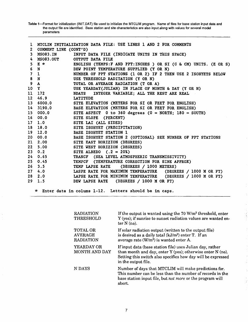
Table 1-Format for initialization {INIT.DAT) file used to initialize the MTCLIM program. Name of files for base station input data and the output file are identified. Base station and site characteristics are also input along with values for several model parameters

1 MTCLIM INITIALIZATION DATA FILE: USE LINES 1 AND 2 FOR COMMENTS 2 COMMENT LINE (CONT'D) 3 MS083.IN INPUT DATA FILE (INDICATE UNITS IN THIS SPACE) 4 MS083.0UT OUTPUT DATA FILE 5 E * ENGLISH (TEMPS:F AND PPT:INCHES ) OR SI (C & CM) UNITS. (E OR S) 6 N DEW POINT TEMPERATURE SUPPLIED (Y OR N) 7 1 NUMBER OF PPT STATIONS (1 OR 2) IF 2 THEN USE 2 ISOHYETS BELOW 8 N USE THRESHOLD RADITATION (Y OR N) 9 A TOTAL OR AVERAGE RADIATION (T OR A)

10 Y USE YEARDAY(JULIAN) IN PLACE OF MONTH & DAY (Y OR N) 11 172 NDAYS INTEGER VARIABLE; ALL THE REST ARE REAL 12 46.9 LATITUDE 13 6000.0 SITE ELEVATION (METERS FOR SI OR FEET FOR ENGLISH) 14 3190.0 BASE ELEVATION (METERS FOR SI OR FEET FOR ENGLISH) 15 000.0 SITE ASPECT 0 to 360 degrees (0 - NORTH; 180 - SOUTH) 16 00.0 SITE SLOPE (PERCENT) 17 1.0 SITE LAI (ALL SIDED) 18 18.0 SITE ISOHYET (PRECIPITATION) 19 12.0 BASE ISOHYET STATION 1 20 00.0 BASE ISOHYET STATION 2 (OPTIONAL) SEE NUMBER OF PPT STATIONS 21 2.00 SITE EAST HORIZION (DEGREES) 22 5.00 SITE WEST HORIZION (DEGREES) 23 0.2 SITE ALBEDO (.2 - 20%) 24 0.65 TRANCF (SEA LEVEL ATMOSPHERIC TRANSMISSIVITY) 25 0.45 TEMPCF (TEMPERATURE CORRECTION FOR SINE APPROX) 26 3.5 TEMP LAPSE RATE (DEGREES I 1000 METERS) 27 4.0 LASPE RATE FOR MAXIMUM TEMPERATURE (DEGREES I 1000 M OR FT) 28 2.0 LAPSE RATE.FOR MINIMUM TEMPERATURE (DEGREES I 1000 M OR FT) 29 1.5 DEW LAPSE RATE (DEGREES I 1000 M OR FT)

* Enter data in colums 1-12. Letters should be in caps.

RADIATION THRESHOLD

TOTAL OR AVERAGE RADIATION

YEARDAYOR MONTH AND DAY

NDAYS

If the output is wanted using the 70 W/m2 threshold, enter Y (yes); if sunrise to sunset radiation values are wanted en­terN (no).

If solar radiation output (written to the output file) is desired as a daily total (kJ/m2) enter T. If an average rate (W/m2) is wanted enter A.

If input data (base station file) uses Julian day, rather than month and day, enter Y (yes); otherwise enter N (no). Setting this switch also specifies how day will be expressed in the output file.

Number of days that MTCLIM will make predictions for. This number can be less than the number of records in the base station input file, but not more or the program will abort.

7

Base Station Characteristics and Selection-Selection of the primary base station to use for MTCLIM is not too critical, except that the data should be of high quality. As noted previously, we used NWS stations because they are fairly well distributed and the data are readily available. Other stations, such as fire weather stations, RAWS, and other sources can be used if data are available for the desired time period. Extrapolations by MTCLIM will likely be more accurate the closer the base station is to the site. A secondary base station may be used for precipitation data. This station should also be as close to the site as possible, but in the opposite direction from the site as the first base station. More details about selection of this station are discussed in the section evaluating the precipitation estimates (page 00). Values for the following parameters are for the primary base station unless noted otherwise.

LATITUDE

BASE-ELEV

BASE1-ISO

This input is in degrees and tenths of degrees on line 12. Lati­tude is often available with the data, or can be obtained fr<;>m maps.

Elevation of the base station in feet or meters (line 14). If not part of the station documentation, it can be estimated from topo­graphic maps.

Long-term average annual precipitation (inches or centimeters) for the primary base station (line 19). If not part of the documen­tation for the station, a value can be obtained from isohyet maps prepared by the Soil Conservation Service.

BASE2-ISO Long-term average annual precipitation (inches or centimeters) for the secondary base station (line 20). If not part of the docu­mentation for the station, a value can be obtained from isohyet maps prepared by the Soil Conservation Service. Enter 0.0 if MTCLIM is run using only the primary station.

Site Characteristics-The site being modeled by MTCLIM can be a specific stand or other designated area, but the site characteristics should be consistent across the area. For example, major differences in elevation, slope, aspect, or Leaf Area Index (LAI) within one site would require the user to consider the area as dif­ferent sites.

SITE-ELEV Elevation in feet or meters (line 13). This is readily available from topographic maps.

SITE-ASPECT Aspect in degrees from north (0°) can be measured either onsite or obtained from topographic maps (line 15).

SITE-SLOPE Slope as percent and measured on the site (line 16). Slope can also be estimated from topographic maps.

SITE-LAI LAI (Leaf Area Index) is a dimensionless value that represents square meters of leaf area per square meter of ground surface (line 17). LAI is a physiological estimate of canopy coverage. Estimates of LAI can be made from stand basal area using equa­tions (Kaufmann and others 1982; Hungerford 1987) or using instruments (Pierce and Running 1988). Figure 2 shows a rela­tionship between basal area and LAI for several species, which can be used to estimate LAI. This relationship is not available for other species but Douglas-fir, grand fir, and western hemlock would be similar to Engelmann spruce and subalpine fir; ponder­osa pine would be similar to lodgepole, but the slope would be slightly higher.

8

STAND BASAL AREA (FT 2•ACRE-1) -

60 o,..... _______ 2~sr-o _______ s .... oo ~

01 I

::E • ('4

! 40 )( w Q z -< w a: < u. 20 ct w

ENGELMANN SPRUCE

Ne

10 )( w Q

!

Figure 2-Effective projected and total leaf area index as a function of stand basal area for three species. This graph and the equations can be used to estimate LAI in the Central and Northern Rocky Mountains (from Kaufmann and others 1982).

..I

..I ct ... 0 ...

0 50 100

STAND BASAL AREA (M 2• HA- 1

)

SITE-ISO

EAST-HORZ WEST-HORZ

SALBDO

Average annual precipitation isohyet (inches) for the site can be ob­tained from isohyet maps prepared by the Soil Conservation Serv­ice if specific data are not available (line 18).

These are angles to the east (line 21) and west (line 22) horizons that are used to truncate direct beam solar irradiance due to blocking by ridges or timber edges. They can be measured degrees onsite or obtained from topographic maps (see appendix E).

Albedo for the site represents the amount (percent) of solar radia­tion reflected by the surface back into the atmosphere (line 23). The value changes with the type of surface material on the site. Some typical values for different materials are given in the follow­ing tabulation (Fowler 1974; Lowry 1969; Rosenberg 1974):

Surface AJbedo

Forest canopy Soils Rock Peat Needles and litter (dry) Bark Grass Chips Charcoal Snow

9

Percent 10-20 20-35 10-30 5-15 6-11

20 20-25

36 2

80-95

Model Adjustments-The model is adjusted by changing the values for the coefficients in the initialization file (lines 24-29). These coefficients adjust clear sky transmissivity, daylight average temperature amplitude, and temperature­elevational relationships. The following discussion describes the parameters, gives starting values, and suggests values for different conditions.

TRANCF Clear sky transmissivity at sea level is needed to calculate solar radia­tion and adjust for cloud cover. For our tests, we assumed TRANCF to be 0.65 and increase it as elevation increases. This value is based on Gates (1980) and Bristow and Campbell (1984) and our testing of the model. It is selected from the range of possible values and is realistic for western Montana.

Turbidity of the atmosphere due to dust, pollutants, and atmospheric constituents such as ozone, oxygen, water vapor, and clouds, cause the variable attenuation of radiation by influencing transmissivity. Thus, TRANCF may be as low as 0.40 at sea level under turbid conditions and as high as 0.80 under very clear conditions at high elevations (Gates 1980). Since the model calculates transmissivity changes due to moisture and clouds, the other factors need to be accounted for. If information is available to suggest a value different from 0.65 for your area, it should be changed. Also, the value of the coefficient can be changed if the information is not available, but a value different from 0.65 is suspected because outputs from this model are different from observed values. This is discussed more later in the section discussing evaluation of MTCLIM.

TEMCF Daylight average coefficient is used in the equation for calculating daylight average temperature (equation 1, page 4). This coefficient adjusts the daylight average temperature above the daily mean. For the western Montana area, where this model was developed, a coeffi­cient value of 0.45 worked well for all sites. This value is input in the initialization (INIT.DAT) file and can be changed if desired. For sites and base stations where the diurnal temperature curve more closely approximates the sine function, the value ofTEMCF will be lower. Assuming the sine wave approximation, the value ofTEMCF is 0.212. Measured temperature data can be used to evaluate TEMCF for a given locale if they are available. See appendix B for details.

TLAPSE Elevationallapse rate used for the daylight average temperature cal­culations. We used a value of 3.5 °F/1,000 ft (6.4 °C/1,000 m) for west­em Montana. This value is based on weather data (Finklin 1983, 1986). If data from other locations indicate a different value, TLAPSE can be changed.

MAXLAP Elevationallapse rate used for maximum temperature calculations. We used a value of 4.5 °F/1,000 ft (8.2 °C/1,000 m) for western Mon­tana which is based on Finklin (1983, 1986). This rate seems to repre­sent an average between mountain and canyon stations during the summer period. Lapse rates are different during the winter (Finklin 1983, 1986). If data from other locations indicate a different value, MAXLAP can be changed.

MINLAP Elevationallapse rate used for minimum temperature calculations. Information for our area suggested that lapse rates are from 1.8 to 3.3 °F/1,000 ft (3.3 to 6.0 °C/1,000 m). (Finklin 1983, 1986). Our unpublished data suggest different rates, depending on whether a site is on a mountain slope, a creek bottom, or a mountain basin. Our re­sults indicate that a value of 0 to 2.0 °F/1,000 ft (0 to 3.8 °C/1,000 m) is appropriate, when moving from valley bottom base stations to

10

MTCLIM Output File

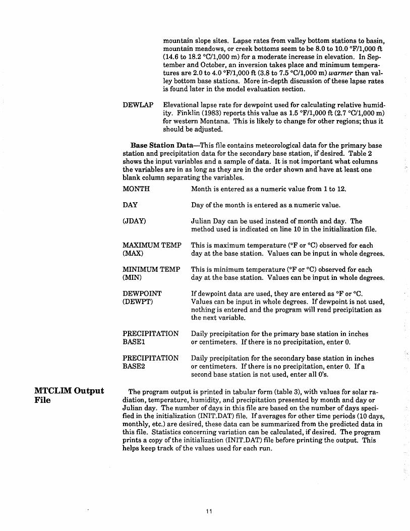
mountain slope sites. Lapse rates from valley bottom stations to basin, mountain meadows, or creek bottoms seem to be 8.0 to 10.0 °F/l,OOO ft (14.6 to 18.2 °C/l,OOO m) for a moderate increase in elevation. In Sep­tember and October, an inversion takes place and minimum tempera­tures are 2.0 to 4.0 °F/l,OOO ft (3.8 to 7.5 °C/l,OOO m) warmer than val­ley bottom base stations. More in-depth discussion of these lapse rates is found later in the model evaluation section.

DEWLAP Elevationallapse rate for dewpoint used for calculating relative humid­ity. Finklin (1983) reports this value as 1.5 °F/l,OOO ft (2. 7 °C/l,OOO m) for western Montana. This is likely to change for other regions; thus it should be adjusted.

Base Station Data-This file contains meteorological data for the primary base station and precipitation data for the secondary base station, if desired. Table 2 shows the input variables and a sample of data. It is not important what columns the variables are in as long as they are in the order shown and have at least one blank column. separating the variables.

MONTH Month is entered as a numeric value from 1 to 12.

DAY

(JDAY)

MAXIMUM TEMP (MAX)

MINIMUM TEMP (MIN)

DEWPOINT (DEWPT)

PRECIPITATION BASEl

PRECIPITATION BASE2

Day of the month is entered as a numeric value.

Julian Day can be used instead of month and day. The method used is indicated on line 10 in the initialization file.

This is maximum temperature (°F or °C) observed for each day at the base station. Values can be input in whole degrees.

This is minimum temperature (°F or °C) observed for each day at the base station. Values can be input in whole degrees.

If dewpoint data are used, they are entered as °F or °C. Values can be input in whole degrees. If dewpoint is not used, nothing is entered and the program will read precipitation as the next variable.

Daily precipitation for the primary base station in inches or centimeters. If there is no precipitation, enter 0.

Daily precipitation for the secondary base station in inches or centimeters. If there is no precipitation, enter 0. If a second base station is not used, enter all O's.

The program output is printed in tabular form (table 3), with values for solar ra­diation, temperature, humidity, and precipitation presented by month and day or Julian day. The number of days in this file are based on the number of days speci­fied in the initialization (INIT.DAT) file. If averages for other time periods (10 days, monthly, etc.) are desired, these data can be summarized from the predicted data in this file. Statistics concerning variation can be calculated, if desired. The program prints a copy of the initialization (INIT.DAT) file before printing the output. This helps keep track of the values used for each run.

11

Table 2-Sample input data file for base station. Headings show the inputs needed and the units. In creating the file, headings will not be input. This sample is for only 1 month. In an actual run these data will need to cover the time period to be predicted

Temperature Precipitation'

MQZ DAY2 MAX MIN DEWPT' BASE1 BASE24

___ oFs ___ - -- - lncfJS - - - -

7 01 78 45 0 0 7 02 81 50 0.34 0 7 03 70 54 .37 0.30 7 04 73 50 .03 .30 7 05 71 51 .18 .15 7 06 77 48 .02 .06 7 07 84 47 0 0 7 08 80 56 0 0 7 09 81 49 .10 .10 7 10 73 49 0 0 7 11 83 43 0 0 7 12 75 55 .23 0 7 13 68 50 .18 .13 7 14 59 45 .09 .05 7 15 75 51 .01 .19 7 16 85 46 0 0 7 17 76 48 0 0 7 18 74 46 0 0 7 19 80 46 0 0 7 20 80 47 0 0 7 21 90 49 0 0 7 22 97 53 0 0 7 23 92 61 0 .01 7 24 87 50 0 0 7 25 88 53 0 0 7 26 87 52 0 0 7 27 89 51 0 0 7 28 92 50 0 0 7 29 87 56 0 0 7 30 92 48 0 0 7 31 89 46 .03 0

1 Enter precipitation as inches or centimeters and specify which in initialization file. 2Julian day may be used instead of month and day. The method used in this file must be

indicated on line 10 of the initialization file. 3 lf dewpoint is not used, nothing is entered. Precipitation will start in these columns instead. 4 lf data for a second base station are not used, zeroes must be entered or the program will

abort. 5The units printed out will depend on whether English or Sl units are specified in the initializa-

tion file.

12

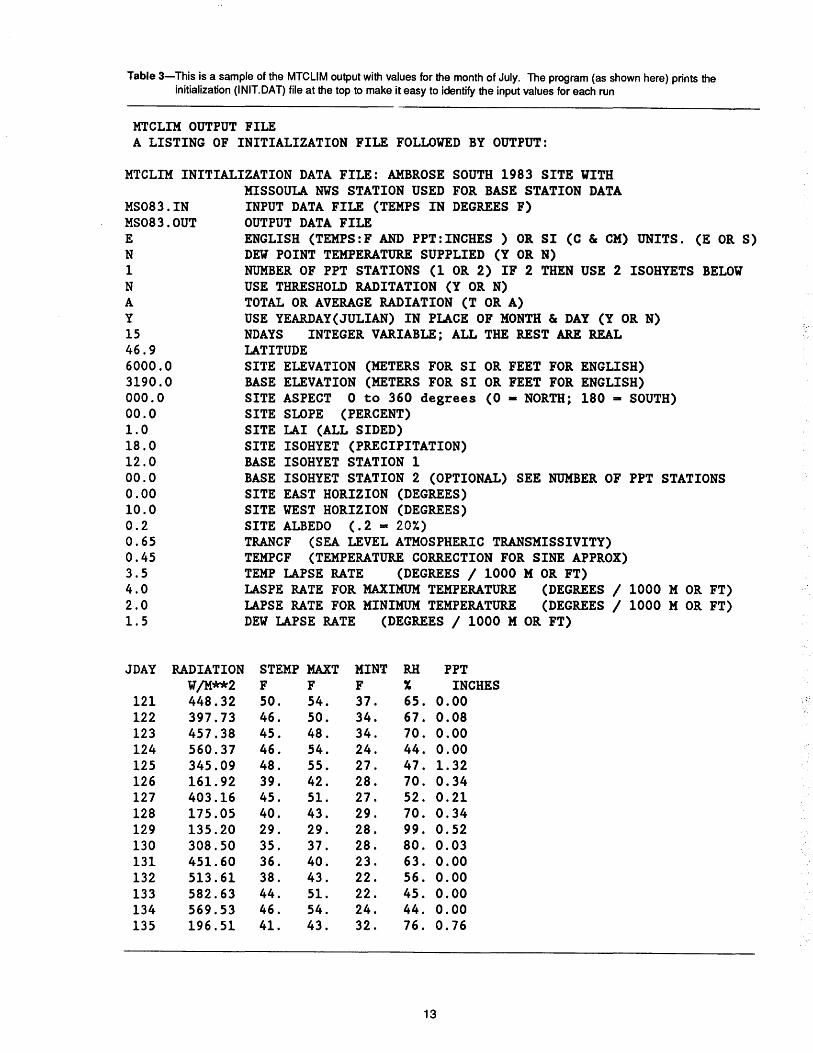
Table 3-This is a sample of the MTCLIM output with values for the month of July. The program (as shown here) prints the initialization (INIT.DAT) file at the top to make it easy to identify the input values for each run

MTCLIM OUTPUT FILE A LISTING OF INITIALIZATION FILE FOLLOWED BY OUTPUT:

MTCLIM INITIALIZATION DATA FILE: AMBROSE SOUTH 1983 SITE WITH

MS083.IN MS083.0UT E N 1 N A y

15 46.9 6000.0 3190.0 000.0 00.0 1.0 18.0 12.0 00.0 0.00 10.0 0.2 0.65 0.45 3.5 4.0 2.0 1.5

JDAY

121 122 123 124 125 126 127 128 129 130 131 132 133 134 135

RADIATION W/M**2 448.32 397.73 457.38 560.37 345.09 161.92 403.16 175.05 135.20 308.50 451.60 513.61 582.63 569.53 196.51

MISSOULA NWS STATION USED FOR BASE STATION DATA INPUT DATA FILE (TEMPS IN DEGREES F) OUTPUT DATA FILE ENGLISH (TEMPS:F AND PPT:INCHES ) OR SI (C & CM) UNITS. (E OR S) DEW POINT TEMPERATURE SUPPLIED (Y OR N) NUMBER OF PPT STATIONS (1 OR 2) IF 2 THEN USE 2 ISOHYETS BELOW USE THRESHOLD RADITATION (Y OR N) TOTAL OR AVERAGE RADIATION (T OR A) USE YEARDAY(JULIAN) IN PLACE OF MONTH & DAY (Y OR N) NDAYS INTEGER VARIABLE; ALL THE REST ARE REAL LATITUDE SITE ELEVATION (METERS FOR SI OR FEET FOR ENGLISH) BASE ELEVATION (METERS FOR SI OR FEET FOR ENGLISH) SITE ASPECT 0 to 360 degrees (0 - NORTH; 180 - SOUTH) SITE SLOPE (PERCENT) SITE LAI (ALL SIDED) SITE ISOHYET (PRECIPITATION) BASE ISOHYET STATION 1 BASE ISOHYET STATION 2 (OPTIONAL) SEE NUMBER OF PPT STATIONS SITE EAST HORIZION (DEGREES) SITE WEST HORIZION (DEGREES) SITE ALBEDO (.2 - 20%) TRANCF (SEA LEVEL ATMOSPHERIC TRANSMISSIVITY) TEMPCF (TEMPERATURE CORRECTION FOR SINE APPROX) TEMP LAPSE RATE (DEGREES I 1000 M OR FT) LASPE RATE FOR MAXIMUM TEMPERATURE (DEGREES I 1000 M OR FT) LAPSE RATE FOR MINIMUM TEMPERATURE (DEGREES I 1000 M OR FT) DEW LAPSE RATE (DEGREES I 1000 M OR FT)

STEMP MAXT MINT RH PPT F F F X INCHES 50. 54. 37. 65. 0.00 46. 50. 34. 67. 0.08 45. 48. 34. 70. 0.00 46. 54. 24. 44. 0.00 48. 55. 27. 47. 1.32 39. 42. 28. 70. 0.34 45. 51. 27. 52. 0.21 40. 43. 29. 70. 0.34 29. 29. 28. 99. 0.52 35. 37. 28. 80. 0.03 36. 40. 23. 63. 0.00 38. 43. 22. 56. 0.00 44. 51. 22. 45. 0.00 46. 54. 24. 44. 0.00 41. 43. 32. 76. 0.76

13

DATE

SOLAR RADIATION (RADIATION)

DAY AVERAGE TEMP (STEMP)

MAXIMUM TEMP (MAXT)

MINIMUM TEMP (MINT)

HUMIDITY (RH)

PRECIPITATION (PPT)

This will be printed as Julian day or month and day based on entry on line 10 of the initialization (INIT.DAT) file.

Solar radiation (table 3) is expressed as either a daily total (in kJ/m2) or an average rate for the day (in W/m2),

depending on user preference. This output will be ex­pressed using the 70 W/m2 threshold value or sunrise to sunset values for daylength.

Temperature averaged over the daylight hours (sunrise to sunset). Outputs can be in degrees C or F (based on entry on line 5 in initialization file).

Daily maximum temperature can be in degrees Cor F (based on entry on line 5 in initialization file).

Daily minimum temperature can be in degrees C or F (based on entry on line 5 in initialization file).

Relative humidity (percent) averaged over the daylight hours (sunrise to sunset).

Daily total precipitation in inches or centimeters (based on entry on line 5 of initialization file).

Executing MTCLIM General Use-Once the initialization (INIT.DAT) and Base Station files have

Procedures

Solar Radiation

been created as described in the previous section, MTCLIM is ready to run, (assum­ing the program is compiled on the machine being used). When the program is started, it will ask for the name of the initialization (INIT.DAT) file. Mter the file name is given, MTCLIM will execute and put the output, as in table 3, in the file designated in the initialization (INIT.DAT) file.

The source code and the executable program can be mailed on the Forest Service Data General System to any system user. The source code, executable files, the ini­tialization (INIT.DAT) file, and some help files are available on 5 1/4-inch floppy discs for IBM and IBM compatible PC's.

EVALUATION OF MTCLIM

To test the accuracy ofMTCLIM calculations, observed data from several sites in western Montana were selected (Hungerford and Babbitt 1987; Hungerford and Schlieter 1984; Running and others 1987). These data, which were not used to de­velop the equations in MTCLIM, were summarized to daylight average, maximum and minimum air temperatures, and daily solar radiation for each of the sites. The observed daily values were compared to daily MTCLIM predictions for May 1 to October 31, using simple linear regression analysis of predicted data versus ob­served data. Table 4 shows the characteristics of nine sites and the base stations used in the analyses. These sites represent a variety of elevations and slope posi­tions. Specific sites used to generate model output are shown in table 5. Details for the precipitation tests are given later.

Because solar radiation data are not available for all sites, our evaluations were limited to the Ambrose S, Ninemne S, and Coram 12 (table 5) sites.

Results for the linear regression analyses of observed and predicted daily radia­tion are shown in table 6 for the three sites. The slope for all three sites (0.65 to 0. 78) is less than 1.0 and the intercepts for all sites are greater than zero. The r 2

values of 0.50 to 0.55 are not as good as desired, but are reasonable considering the

14

Table 4-General characteristics of study sites and base stations

Distance to Site Aspect Slope Elevation base station

Degrees Percent Feet Miles Lubrecht ( clearcut) 0 0 4,000 32 Coram 14 (uncut) 112 60 4,400 15 Coram 12 ( clearcut) 112 50 4,350 15 Coram 33 (clearcut) 270 5 3,950 15 Ambrose N 350 40 6,000 32 Ambrose S 195 50 6,000 32 Ninemile N 330 40 5,600 25 Ninemile S 170 50 5,600 25 Schwartz N 40 40 5,000 19 Kalispell Base 0 0 2,965 0 Missoula Base 0 0 3,190 0

Table 5-Sources of data used for evaluation of each model output

Temperature

Site Radiation Day Maximum Minimum Humidity

Lubrecht X X X

Coram 14 X X

Coram 12 X X X X

Coram 33 X X X

Ambrose N X X X

Ambrose S X X X X

Ninemile N X X

Ninemile S X X X X

Schwartz N X X

Table &-Predicted vs. observed solar radiation comparisons for three sites using linear regression analysis

Site Intercept Slope rz SEE1 n

Ambrose S2 102 0.78 0.55 102 174 Ambrose S2 0 .98 .50 106 174 Ninemile S2 143 .65 .50 104 146 Ninemile S2 0 .93 .40 114 146 Coram 123 5.6 .74 .50 4.4 184 Coram 123 0 1.07 .38 4.8 184

1Standard error of the estimate. 2W/m2• 3ln mJ/m2•

variation in cloud cover between the base stations and sites. Figure 3 shows a plot of predicted vs. observed daily radiation for Ambrose S compared to the 1:1 line. It shows that the model overpredicts for cloudy days and underpredicts for clear days. When the intercepts for the regression are forced through the origin, the slopes are much closer to 1.0 (table 6). In this constrained regression, the standard error of the estimate increases slightly and r2 drops (table 6). Although the statistics are not quite as good for the constrained regression, having the intercept through the origin is much more realistic. This analysis shows that we slightly underestimated radia­tion at Ambrose S (fig. 3) and Ninemile S, while the model overestimated radiation

15

..

at Coram 12. Figure 4 shows the daily comparison of predicted and observed solar radiation for the Ninemile site. Only 2 out of every 3 days are plotted. The close­ness of the lines indicate that predicted and observed solar radiation values are close for most days.

Evaluation of outlying values and residuals in figure 3 indicated that most over­predictions were the result of cloudier conditions at the mountain site than at the base station. We frequently observed that when it was partly cloudy at valley loca­tions, clouds were stacked up against the mountains; thus, predictions using base station data in valley bottoms will overpredict at mountainous sites. Analysis of underpredictions revealed that these occurred on days when weather was chang­ing; thus, the temperature amplitude was small. As a result, the model simulated cloudy skies when skies were actually clear; thus, the predicted radiation is low (see appendix A for details of calculation).

700

600 ,........ N 500 E

• • ' 3: 400 ......_

• •• • • • • • • • a w 300 1-

u 0

• • • .. • • • • •

w 200 0::: • Y = 102 + .78X • •

a..

100 • • 0

0 100

• • •• •

• •

200 300 400 500

OBSERVED {W/m2)

Figure 3-Regression of incoming solar radiation predicted by MTCLIM vs. actual radiation observed at Ambrose S. Broken line is the regression line and the solid line is the 1 :1 line (intercept= 0; slope = 1.0).

-N E

......... ~ .........,

z 0

~ 0 ~ 0::: a::: ~ 0 Vl

700

600

500

400

300

200

100

0

-OBSERVED .... PREDIC'Tm

.. . .

150 175 200 225 250 275

YEAR DAY

Figure 4---Comparison of observed (solid line) and MTCLIM estimated (broken line) daily solar radiation at Ninemile S.

16

r2 = 0.55 SEE= 102

600 700

300

Temperature

Predictions of radiation from this model using data from valley bottom stations are reasonably accurate when averaged over a season, but daily predicted values can be quite different from observed values. Predictions can be improved signifi­cantly if base station input data are used from a mountain location or a site very close to the site being predicted (Bristow and Campbell 1984). This would reduce the errors introduced by differences in cloud cover from valley bottom to mountain sites. Underprediction errors resulting from small temperature amplitudes that predict cloud cover when it is actually clear will be created by MTCLIM regardless of choice of base station. Fortunately this situation occurs infrequently.

Evaluations of the temperature predictions are also made using linear regression analysis of predicted and observed temperatures. Analyses of day average and maximum and minimum temperature will be discussed separately.

Daylight Average Temperature-Results of the predicted vs. observed regres­sions are given in table 7 for day average temperature on all nine sites. Overall, ac­curacy is about 4 °F, with intercepts from 0.5 to 2.3, slopes from 0.83 to 1.03, and r2 ranging from 0.87 to 0.93. A typical plot of predicted vs. observed points about the 1: 1line is shown in figure 5. A small but consistent bias of overestimating low tem­peratures and underestimating higher temperatures is evident in these statistics, and was caused by the lapse rate chosen (3.5). But the lapse rate that was chosen appears to be the best compromise for our study area. Other lapse rates would cause greater errors at the higher or lower temperatures. Figure 6 shows a com­parison of observed and predicted daylight average temperatures for Ninemile S. Only 2 out of every 3 days is plotted. The closeness of the lines indicate that pre­dicted and observed temperature values are close for most days. Standard errors of the estimate (table 7) for the predicted and observed regressions range from 1.6 to 2.1 °C.

Table 7-Predicted vs. observed daylight average temperature comparisons for nine sites using linear re-gression analysis. A lapse rate of 3.5 °F/1 ,000 feet was used

Location Year Intercept Slope ~ SEE1 n

oc oc Lubrecht 1980 2.3 0.89 0.92 1.6 131 Coram 14 1976 1.5 .98 .89 1.6 160 Coram 33 1976 1.6 1.03 .88 1.9 174 Coram 12 1976 1.5 .93 .87 1.8 163 Ambrose N 1983 .5 .89 .89 2.1 174 Ambrose S 1983 1.1 .91 .89 2.1 174 Ninemile N 1983 1.7 .92 .89 2.0 146 Ninemile S 1983 1.0 .97 .90 2.0 146 Schwartz N 1983 .8 .83 .93 1.6 172

1Standard error of the estimate.

17

30

25

20 0

0

0 w ... 15 0 E w a: A.

10

5

0

1\ Y:1.1 + .91X

r1:0.B9

SEE: 2.1

n:174

•

•

5

• •

•

10 15 20 25

OBSERVED, °C

Figure 5-Regression of daylight average temperature predicted by MTCLIM on observed daylight average temperature at Ambrose S. Broken line is the regression line and the solid line is the 1 :1 line (intercept= 0; slope = 1.0).

0 0

ui a: ::) 1-< a: w a. :& w .... a: :;( w CJ c( a: w > cC

30

20

10

~ •' •' •' •• ,. '' •' I '

, I

I

30

.... ::c 0 :i >­< 0 0~--------------------------~--~--------~

150 200 250

YEARDAY

Figure &-Comparison of observed (solid line) and MTCLIM estimated (bro­ken line) daily daylight average temperature at Ninemile S.

18

300

Maximum Temperature-Results of the predicted vs. observed regressions for maximum temperature are given in table 8 for five sites. Overall, accuracy is about 4 °F, with intercepts from -0.69 to 2.6, slopes from 0.91 to 1.03, and r 2 ranging from 0.86 to 0.94. A typical plot of predicted vs. observed points about the 1:1line is shown in figure 7. A small but consistent bias of overestimating low temperatures and underestimating higher temperatures is also evident in these statistics. As with the daylight average temperatures, this is caused by the lapse rate chosen (4.5). In some situations a lapse rate of up to 7.0 °F/1,000 ft may be appropriate. The lapse rate of 4.5 °F/1,000 ft, however, seems to be the best compromise for our study area in general. Figure 8 shows a comparison of observed and predicted maxi­mum temperatures. Only 1 out of every 2 days is plotted. The closeness of the lines indicate that predicted and observed temperature values are close for most days. Standard errors of the estimate (table 8) for the regressions are 1.6 to 2.4.

Table 8-Predicted vs. observed maximum temperature comparisons for five sites using linear regression analysis

Location Year MAX LAP Intercept Slope til

°F/1,000 ft oc Lubrecht 1980 4.5 0.56 0.94 0.94 Coram 33 1976 4.5 2.6 .92 .89 Coram 12 1976 4.5 2.1 .91 .86 Coram 14 1976 4.5 2.0 1.03 .92 Ambrose S 1983 4.5 -.69 .96 .89

1Standard error of the estimate.

35 /1. Y: 2.1 + .91 X

r 2.: 0.86

30 SEE: 2.3

n:172

25 (.)

0

Q 20 UJ ... ~ c w 15 a: A. •

• 10 • • •

5

0 5 10 15 20 25 30

OBSERVED,°C

Figure 7-Regression of maximum temperature predicted by MTCLIM on observed maximum temperature at Coram 12. Broken line is the regression line and the solid line is t:,e 1 :1 line (intercept= 0; slope= 1.0).

19

SEE1

oc 1.6 2.1 2.3 1.7 2.4

35

n

131 175 172 173 174

:"!'-

0~------------------._----~------~----_.----~ 170 190 210 230 250 270

YEARDAY

Figure &-Comparison of observed (broken line) and MTCLIM esti­mated (solid line) daily maximum temperature at Lubrecht. Every other day is plotted.

290 310

Minimum Temperature-Due to the effect of frost pockets, cold air drainage, and temperature inversions, prediction of minimum temperatures was difficult. Information for our area (Finklin 1983) suggested that the lapse rate for minimum temperatures is between 1.8 and 3.3 °F/1,000 ft; therefore we chose 2.0 for our ini­tial analysis. It became apparent right away that the accuracy of our MTCLIM minimum temperature predictions varied from less than 3 to 6 °F depending on site (table 9). The lapse rate of 2.0 °F/1,000 ft was not high enough for Lubrecht and Coram 33, which are basin or creek bottom locations that trap cold air. In some cases, the lapse rate was too high for slope sites. Comparison of the predicted and observed data also revealed that lapse rates sometimes reverse after September 1. These three situations will be discussed separately.

MTCLIM predictions at a basin location (Lubrecht) and a creek bottom station (Coram 33) were quite close to observed temperatures when a lapse rate of 10 °F/ 1,000 ft was used (table 9). At Lubrecht the intercept is close to zero and the slope is nearly 1.0 and r2 = 0.91. At Coram 33 the r2 is 0.70, with the intercept at -1.1 and the slope at 0.98. These statistics suggest that the lapse rate is a little high at Coram 33; it may be closer to 8.0 °F/1,000 ft. Because both of these stations are only 1,000 feet in elevation above the valley bottom base stations, a lapse rate of 10 °F/1,000 ft may predict temperatures lower than observed at locations with greater elevation differences relative to the base station. In the event that data from a slope base station are input to MTCLIM to predict minimum temperatures in a creek bottom or basin location, the lapse rate of 10 °F/1,000 ft is appropriate.

MTCLIM predictions on mountain slopes using lapse rates of 0 to 2.0 °F/1,000 ft are reasonably close to observed temperatures. Results of regressions from Coram 12, Ambrose N, and Ninemile S (table 9) show that the predictions using a lapse of zero give the best compromise considering predictions over the whole range of tem­peratures (fig. 9). The r2 values 0.56 to 0.75 show that considerable daily variation exists between predicted and observed values. The slope of these relationships is not as close to 1.0 as we would like (except for Ninemile Sat 0.97). For our area

20

Table 9-Predicted vs. observed minimum temperature comparisons for five sites using linear regression analysis. Two lapse rates are analyzed for each site

Location Year MINLAP Intercept Slope

°FI1,000 ft oc Lubrecht 1980 10.0 0.10 1.05

2.0 3.70 1.05

Coram 33 1976 10.0 -1.10 .98 2.0 3.28 .98

Coram 12 1976 2.0 .76 .76 0 2.29 .76

Ambrose N 1983 2.0 -.39 .77 0 2.70 .77

Ninemile S 1983 2.0 -1.50 .97 0 .95 .97

1Standard error of the estimate.

15 /+. Y=2.7 + .77X •

0 0

0 w t­(.)

E w £C 0.

10

5

0

-10

r2= 0.61 SEE: 3.3

n =174

-5

• •

•

• • •

' •

0 5

OBSERVED,°C

•

• •

10

Figure 9-Regression of minimum temperature predicted by MTCLIM on observed minimum temperature at Ambrose N. Broken line is the re­gression line and the solid line is the 1 :1 line (intercept = 0; slope = 1.0).

,a

0.91

•

.91

.70

.70

.56

.56

.61

.61

.75

.75

• •

• • •

SEE1 n

oc 1.5 131 1.5 131

2.1 116 2.1 116

2.8 118 2.8 118

3.3 174 3.3 174

2.7 145 2.7 145

15

these results suggest that a lapse rate between 0 and 2.0 °F/1,000 ft applied to val­ley bottom base stations will be adequate for predicting minimum temperatures on slope sites from May 1 to September 1.

The analysis of predicted and observed regressions also indicates that minimum temperature on slopes in September and October are often warmer than at valley bottom base stations. Our data indicate an inversion of +2.0 to +4.0 °F. This tem­perature inversion period was not accounted for in our analysis (we used the whole period from May 1 to October 31), therefore the lapse rates for minimum tempera­ture (MINLAP) include the inversion situations. More accurate predictions would likely result if different lapse rates were input for September and October.

21

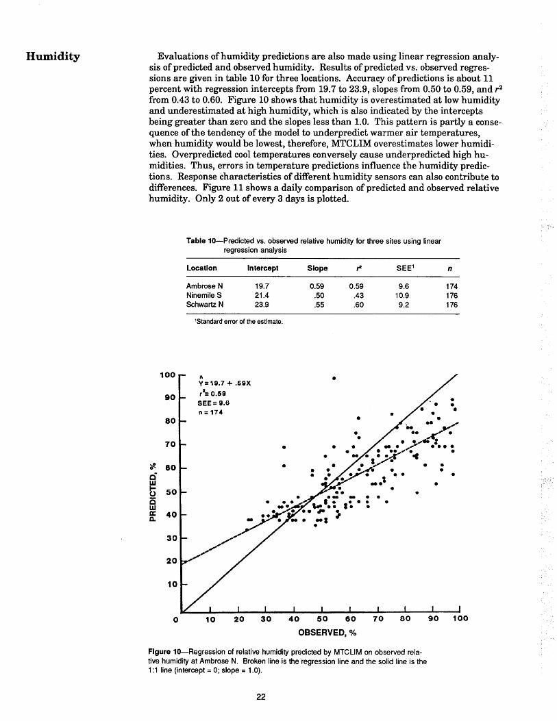
Humidity Evaluations of humidity predictions are also made using linear regression analy­sis of predicted and observed humidity. Results of predicted vs. observed regres­sions are given in table 10 for three locations. Accuracy of predictions is about 11 percent with regression intercepts from 19.7 to 23.9, slopes from 0.50 to 0.59, and r2

from 0.43 to 0.60. Figure 10 shows that humidity is overestimated at low humidity and underestimated at high humidity, which is also indicated by the intercepts being greater than zero and the slopes less than 1.0. This pattern is partly a conse­quence of the tendency of the model to underpredict warmer air temperatures, when humidity would be lowest, therefore, MTCLIM overestimates lower humidi­ties. Overpredicted cool temperatures conversely cause underpredicted high hu­midities. Thus, errors in temperature predictions influence the humidity predic­tions. Response characteristics of different humidity sensors can also contribute to differences. Figure 11 shows a daily comparison of predicted and observed relative humidity. Only 2 out of every 3 days is plotted.

100

90

80

70

~ 0 80 c w 1- 50 0 5 w a: 40 c.

30

20

10

0

Table 10-Prec:licted vs. observed relative humidity for three sites using linear regression analysis

Location Intercept

Ambrose N 19.7 Ninemile S 21.4 Schwartz N 23.9

1Standard error of the estimate.

" Y=19.7 + .59X

r1: 0.59

SEE=9.6 n= 174

• •

Slope

0.59 .50 .55

•

,a

0.59 .43 .60

• • •

SEE1

9.6 10.9 9.2

• •

n

174 176 176

• • • .. •• y''

• .. ,~' . . ., .. : . .. . ,,.., .... . . ..,, . .

.. • • • ... r ., • . ~ ... ,'• • • ..1i • . . . .,.,. . . . ~, -·'

.,~.·. . . ·- - .. •

• •

• • •

• .• • .,_,., ._. I •: I~ • ~ . ,,. . . ,. . •

~ .-•' .,, /'

,/

10 20 30 40 50 60 70 80 90 100

OBSERVED,%

Figure 10-Regression of relative humidity predicted by MTCLIM on observed rela­tive humidity at Ambrose N. Broken line is the regression line and the solid line is the 1 :1 line (intercept = 0; slope = 1.0).

22

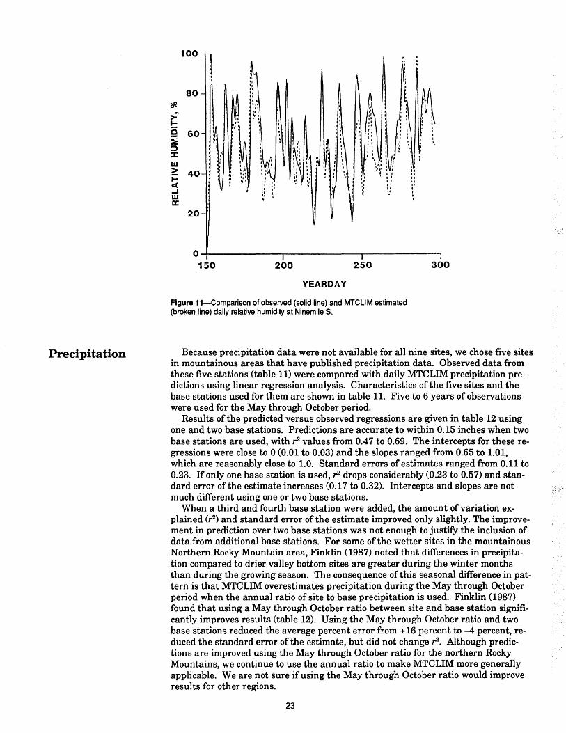
Precipitation

100

80 I I

?/}. lo lu

'" Ill

> ~ I 'I

1- I

e 60 ~ :::) :r: ' w " I

I I : I I

> 40 .... I II! " Ill I I I I ,, .... 'I' IJ II

~ ~ II II

<( ,, •, " I '• 'I ..

..J ~

~: •,

" w ~ . a: ' I

20-

0~------------~------------~----------~

150 200 250

YEARDAY

Figure 11-Comparison of observed (solid line) and MTCLI M estimated (broken line) daily relative humidity at Ninemile S.

300

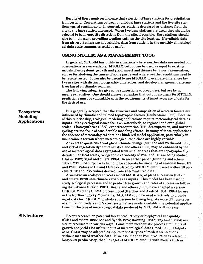
Because precipitation data were not available for all nine sites, we chose five sites in mountainous areas that have published precipitation data. Observed data from these five stations (table 11) were compared with daily MTCLIM precipitation pre­dictions using linear regression analysis. Characteristics of the five sites and the base stations used for them are shown in table 11. Five to 6 years of observations were used for the May through October period.

Results of the predicted versus observed regressions are given in table 12 using one and two base stations. Predictions are accurate to within 0.15 inches when two base stations are used, with r values from 0.47 to 0.69. The intercepts for these re­gressions were close to 0 (0.01 to 0.03) and the slopes ranged from 0.65 to 1.01, which are reasonably close to 1.0. Standard errors of estimates ranged from 0.11 to 0.23. If only one base station is used, r drops considerably (0.23 to 0.57) and stan­dard error of the estimate increases (0.17 to 0.32). Intercepts and slopes are not much different using one or two base stations.

When a third and fourth base station were added, the amount of variation ex­plained (r) and standard error of the estimate improved only slightly. The improve­ment in prediction over two base stations was not enough to justify the inclusion of data from additional base stations. For some of the wetter sites in the mountainous Northern Rocky Mountain area, Finklin (1987) noted that differences in precipita­tion compared to drier valley bottom sites are greater during the winter months than during the growing season. The consequence of this seasonal difference in pat­tern is that MTCLIM overestimates precipitation during the May through October period when the annual ratio of site to base precipitation is used. Finklin (1987) found that using a May through October ratio between site and base station signifi­cantly improves results (table 12). Using the May through October ratio and two base stations reduced the average percent error from +16 percent to -4 percent, re­duced the standard error of the estimate, but did not changer. Although predic­tions are improved using the May through October ratio for the northern Rocky Mountains, we continue to use the annual ratio to make MTCLIM more generally applicable. We are not sure if using the May through October ratio would improve results for other regions.

23

Table 11-Characteristics of locations and base stations used for evaluating the precipitation subroutine

30-year average Distance and Site Elevation annual precipitation direction to site

Feet Inches Garnet, MT 6,060 26.3

Missoula, MT (base 1) 3,190 13.3 36mi E Seeley Lake, MT (base 2) 4,100 22.1 28 mi SSE

Bozeman 12 N E, MT 5,950 34.8

Belgrade, MT (base 1) 4,451 13.8 Bozeman, MT -MSU (base 2) 4,856 18.6

Summit, MT 40.0

Kalispell, MT (base 1) 2,965 15.9 40miE East Glacier, MT (base 2) 4,806 30.5 12 mi SW

Deception Creek, ID 3,060 55.8

Coeur d'Alene, ID (base 1) 2,158 25.8 14 mi ENE Kellogg, ID (base 2) 2,305 30.4 21 mi NW

Pierce, ID 3,185 43.6

Orofino, ID (base 1) 1,027 25.4 21 mi E Elk River, ID (base 2) 2,918 38.5 27mi SE

Table 12-Predicted vs. observed precipitation comparisons for five sites using linear regression analysis. Results are given using 1 and 2 base stations, the annual and May through October ratios of precipitation between site and base stations

Annual ratio May-October ratio

Location Intercept Slope r2 SEE Intercept Slope r2 SEE

Garnet

1 Base 0.03 0.84 0.30 0.22 0.03 0.70 0.30 0.19 2 Base .02 .80 .47 .15 .02 .77 .49 .14

Bozeman 12NE

1 Base .02 1.04 .35 .32 .02 .72 .35 .22 2 Base .02 1.01 .50 .23 .02 .72 .51 .16

Summit ~ ·~ :· ··:

1 Base .05 .73 .23 .27 .03 .49 .23 .18 2 Base .03 .84 .54 .16 .02 .65 .59 .11

Deception Creek

1 Base .03 .94 .57 .22 .03 .78 .57 .18 2 Base .03 .89 .68 .17 .03 .73 .68 .14

Pierce

1 Base .01 .94 .57 .18 .01 .89 .57 .17 2 Base .01 .83 .68 .12 .01 .84 .69 .12

24

Ecosystem Modeling Applications

Silviculture

Results of these analyses indicate that selection of base stations for precipitation is important. Correlations between individual base stations and the five site sta­tions varied considerably. In general, correlations decreased as distance from the site to the base station increased. When two base stations are used, they should be selected to be in opposite directions from the site, if possible. Base stations should also be in the same prevailing weather path as the site location. If available data from airport stations are not suitable, data from stations in the monthly climatologi­cal data state summaries could be useful.

USING MTCLIM AS A MANAGEMENT TOOL

In general, MTCLIM has utility in situations where weather data are needed but observations are unavailable. MTCLIM output can be used as input to existing models of ecosystems, growth and yield, insect and disease behavior, regeneration, etc., or for studying the causes of some past event where weather conditions need to be reconstructed. It can also be useful to use MTCLIM to evaluate differences be­tween sites with distinct topographic differences, and develop management alterna­tives based on climatic regimes.

The following categories give some suggestions of broad uses, but are by no means exhaustive. One should always remember that output accuracy for MTCLIM predictions must be compatible with the requirements of input accuracy of data for the desired use.

It is gen.erally accepted that the structure and composition of western forests are influenced by climatic and related topographic factors (Daubenmire 1956). Because of this relationship, ecological modeling applications require meteorological data as inputs. Many ecological issues focus on watersheds, to regional and even global scales. Photosynthesis (PSN), evapotranspiration (ET), decomposition, and nutrient cycling are the focus of considerable modeling efforts. In many of these applications the absence of meteorological data has hindered model application, particularly in mountainous terrain where meteorological conditions are highly variable.

Answers to questions about global climate change (Manabe and Wetherald 1980) and global vegetation dynamics (Justice and others 1985) may be enhanced by the use of meteorological data aggregated from smaller areas that are topographically detailed. At local scales, topographic variability of PSN and ET are being studied (Hasler 1982; Segal and others 1985). In an earlier paper (Running and others 1987), MTCLIM output was found to be adequate for modeling of seasonal forest ET and PSN. Values of ET and PSN calculated by MTCLIM output were within 10 per­cent of ET and PSN values derived from site-measured data.

A well-known ecological process model (JABOWA) of plant succession (Botkin and others 1972) uses climate variables as inputs. This model has been used to study ecological processes and to predict tree growth and rates of succession follow­ing disturbance (Botkin 1981). Keane and others (1989) have adapted a version (FIRESUM) of the SILVA process model (Kercher and Axelrod 1981, 1984) for use in the Northern Rocky Mountains. MTCLIM could be used effectively to provide input data for FIRESUM to study succession following fire. As more of these types of simulation models and "expert systems" are made available; the potential applica­tions for the type of meteorological data produced by MTCLIM will increase.

Recent research on potential forest productivity or biophysical site quality (Giles and others 1985; Lee and Sypolt 1974; Running 1984b; Tajchman 1984) use site microclimate in various ways. Some more mechanistic process simulators of growth and yield also utilize inputs of meteorological data (Reed 1980). Outputs of MTCLIM may be adapted as inputs to these types of models for locations without measured weather data. If we assume that PSN production is related to long-term productivity, then linkages ofMTCLIM outputs with models such as

25

Fire

Hydrology

DA YTRANS/PSN (Running 1984a, 1984b) give us a way to evaluate relative pro­ductivity of sites. Running (1984b) used a computer simulation for different envi­ronments to evaluate the effects of microclimate on productivity. Running and others (1987) found that small differences in weather made significant differences in PSN. These PSN differences were often related to aspect. Tesch (1981) found significant differences in productivity between north and south slopes. The ability exists to evaluate site response and alternative silvicultural prescriptions by using MTCLIM linked to growth simulation models such as FIRESUM (Keane and others 1987) and DAYTRANS/PSN (Running 1984b).

Meteorological parameters such as temperature, solar radiation, humidity, and precipitation are typically very important in the mountainous west for evaluating regeneration potential. Values for these variables from MTCLIM can be helpful to managers in selecting species for planting, evaluating site regeneration potential, selection of cutting and regeneration methods, and identifying problem sites.

Habitat types (Pfister and others 1977) are used to identify units of land that are similar, based on the assumption that the vegetation integrates the variation in environmental conditions. Typical weather stations are identified in the habitat classifications, but, with most stations located in valley bottoms, representative data are lacking for most habitat types. The MTCLIM model could be used to study weather variations within a habitat type or between habitat types by simu­lating data for a number of locations representative of the desired types. Under­standing some of this variability may be useful in developing silvicultural prescriptions.

The potential for regeneration success could be evaluated using MTCLIM. Runs of the model for sites with regeneration successes could be compared with runs for sites with failures, to identify critical parameters. Critical differences in heat stress, frost, moisture stress, and radiation loads may be identified. Upon identifi­cation of critical factors, mitigation methods should be identifiable. MTCLIM may be useful for evaluating regeneration potential of sites and aiding in formulation of silvicultural prescriptions.

Weather data are very important for evaluating hazard potential, determining fire behavior, and writing prescriptions for controlled bums. The importance of weather data is evidenced by the development ofNFDRS (Furman and Brink 1975), and the BEHAVE model (Andrews 1986). Many recent advances in meteoro­logical tools and models (Fox and others 1985) aid the man?ger in obtaining inputs to do a better job of fire planning and management. While measurement systems through NFDRS and RAWS stations (Warren and Vance 1981) supply managers with much-needed data, the expense and logistics do not allow data measurement at all locations. We believe that MTCLIM outputs can be used to fill in the ''holes" in actual weather data by extrapolating data from locations where measurements are available. Some of the subroutines in MTCLIM, such as radiation and tem­perature, may also be useful for calculating duff moisture for input into BEHAVE. The MTCLIM model should complement the already existing methods of data col­lection and the fire models available to managers, particularly in regions of com­plex topography.

MTCLIM extrapolations of weather data should be very useful for evaluating precipitation and ET potential for sites without measured weather data. Evalu­ations of MTCLIM output for ET calculations (Running and others 1987) indicate good results. Linkages of MTCLIM to ecosystem models described earlier for evaluating vegetation development should also help in assessing treatment-related effects on site water balance. MTCLIM outputs of solar radiation and temperature should also be useful for evaluating site and treatment differences in snowmelt.

26

Insects and Disease

Weather and microclimate differences are often related to insect activity (Amman 1978). MTCLIM outputs should be helpful in assessing site-specific insect activity and linking to available insect models. Disease activity is also directly re­lated to weather and microclimate differences (McDonald and others 1987a, 1987b; Waggoner 1975); thus MTCLIM output could be valuable in assessing epide~iology of a variety of forest diseases. There is some indication that climatic stress (mois­ture and temperature) is important to pathogenicity of root rot caused by Armillaria spp. in the Northern Rocky Mountains (McDonald and others 1987b). MTCLIM may be useful in helping to understand the site-disease relationships.

REFERENCES Amman, Gene D. 1978. The biology, ecology and causes of outbreaks ofthe

mountain pine beetle in lodgepole pine forests. In: Kibbee, Darline L.; Berryman, Alan A.; Amman, Gene D.; Stark, Ronald W., eds. Theory and practice of moun­tain pine beetle management in lodgepole pine forests: symposium proceedings; 1978 April25-27; Pullman, WA Moscow, ID: University of Idaho. Forest, Wildlife, and Range Experiment Station: 39-53.

Andrews, Patricia L. 1986. BEHAVE: fire behavior prediction and fuel modeling system-BURN subsystem, Part 1. Gen. Tech. Rep. INT-194. Ogden, UT: U.S. Department of Agriculture, Forest Service, Intermountain Research Station. 130p.

Baker, F. S. 1944. Mountain climates ofthe western United States. Ecological Monographs. 14(2): 225-254.

Botkin, D. B. 1981. Causality and succession. In: West, D. C.; Shugart, H. H.; Botkin, D. B., eds. Forest succession: concepts and application. New York: Springer-Verlag: 36-55.

Botkin, D. B.; Janak, J. F.; Wallis, J. R. 1972. Some ecological consequences of a computer model of forest growth. Ecology. 60:849-872.

Bristow, K L.; Campbell, G. S. 1984. On the relationship between incoming solar radiation and daily maximum and minimum temperature. Agricultural and For­est Meteorology. 31: 159-166.

Buffo, J.; Fritschen, L.; Murphy, J. 1972. Direct solar radiation on various slopes from 0° to 60° north latitude. Res. Pap. PNW-142. Portland, OR: U.S. Department of Agriculture, Forest Service, Pacific Northwest Forest and Range Experiment Station. 7 4 p.

Daubenmire, R. 1956. Climate as a determinate ofvegetation distribution in eastern Washington and northern Idaho. Ecological Monograph. 26: 131-154.

Denmead, 0. T.; Bradley, E. F. 1985. Flux-gradient relationships in a forest canopy. In: Hutchison, B. A.; Hicks, B. B., eds. The forest-atmosphere interaction. Hingham, MA: D. Reidel Publishing Co: 421-442.

Fink lin, A. I. 1983. Climate of Priest River Experimental Forest, northern Idaho. Gen. Tech. Rep. INT-159. Ogden, UT: U.S. Department of Agriculture, Forest Service, Intermountain Forest and Range Experiment Station. 53 p.

Finklin, A. I. 1986. A climatic handbook for Glacier National Park-with data for Waterton Lakes National Park. Gen. Tech. Rep. INT-204. Ogden, UT: U.S. Department of Agriculture, Forest Service, Intermountain Research Station. 124 p.

Fink lin, A. I. 1987. Procedure for estimating daily precipitation: summary of test results. Unpublished paper on file at: U.S. Department of Agriculture, Forest Service, Intermountain Research Station, Fire Sciences Laboratory, Missoula, MT; RWU -4403 files.

Fowler, W. B. 1974. Microclimate. In: Cramer, Owen P., ed. Environmental effects of forest residues management in the Pacific Northwest: a state of knowledge compendium. Gen. Tech. Rep. PNW-24. Portland, OR: U.S. Department of Agriculture, Forest Service, Pacific Northwest Forest and Range Experiment Station: N1-N18.

27

Fox, Douglas G.; Blankenship, James 0.; Dietrich, David L. 1985. Meteorological tools for wilderness fire management. In: Lotan, James E.; Kilgore, Bruce M.; Fischer, William C.; Mutch, Robert W., tech. coords. Proceedings, symposium and workshop on wilderness fire; 1983 November 15-18; Missoula, MT. Gen. Tech. Rep. INT-182. Ogden, UT: U.S. Department of Agriculture, Forest Service, Inter­mountain Forest and Range Experiment Station: 333-341.

Furman, R. W.; Brink, G. E. 1975. The National Fire Weather Data Library: what it is and how to use it. Gen. Tech. Rep. RM-19. Fort Collins, CO: U.S. Department of Agriculture, Forest Service, Rocky Mountain Forest and Range Experiment Station. 9 p.

Gamier, B. J.; Ohmura, A 1968. A method of calculating the direct shortwave ra­diation income of slopes. Journal of Applied Meteorology. 7(5): 796-800.

Gates, David M. 1980. Biophysical ecology. New York: Springer-Verlag. 611 p. Giles, D. G.; Black, T. A; Spittlehouse, D. L. 1985. Determination of growing sea­

son soil water deficits on a forested slope using water balance analysis. Canadian Journal of Forest Research. 15: 107-114.

Hasler, R. 1982. Net photosynthesis and transpiration of Pinus montana on east and north facing slopes at alpine timberline. Oecologia. 54: 14-22.

Hungerford, Roger D. 1987. Estimation of foliage area in dense Montana lodgepole pine stands. Canadian Journal of Forest Research. 17: 320-324.

Hungerford, Roger D.; Babbitt, Ronald E. 1987. Overstory removal and residue treatments affect soil surface, air, and soil temperature: implications for seedling survival. Res. Pap. INT-377. Ogden, UT: U.S. Department of Agriculture, Forest Service, Intermountain Research Station. 19 p.

Hungerford, Roger D.; Schlieter, Joyce A 1984. Weather summaries for Coram Ex­perimental Forest, northwestern Montana-an International Biosphere Reserve. Gen. Tech. Rep. INT-160. Ogden, UT: U.S. Department of Agriculture, Forest Service, Intermountain Forest and Range Experiment Station. 34 p.

Jarvis, P. G.; Leverenz, J. L. 1983. Productivity of temperate, deciduous and ever­green forests. In: Lange, 0. L.; Nobel, P. S.; Osmond, C. B.; Ziegler, H., eds. Ency­clopedia of plant physiology. Vol. 12D: Physiological plant ecology IV. Berlin: Springer-Verlag: 233-280.

Justice, C. 0.; Townshend, J. R. G.; Holben, B. N.; Tucker, C. J. 1985. Analysis of the phenology of global vegetation using meteorological satellite data. Interna­tional Journal of Remote Sensing. 6(8): 1271-1318.

Kaufmann, M. R. 1984. Effects of weather and physiographic conditions on tem­perature and humidity in subalpine watersheds of the Fraser Experimental Forest. Res. Pap. RM-251. Fort Collins, CO: U.S. Department of Agriculture, Forest Service, Rocky Mountain Forest and Range Experiment Station. 9 p.

Kaufmann, M. R.; Edminster, C. B.; Troendle, C. A. 1982. Leaf area determinations for subalpine tree species in the Central Rocky Mountains. Res. Pap. RM-238. Fort Collins, CO: U.S. Department of Agriculture, Forest Service, Rocky Moun­tain Forest and Range Experiment Station. 7 p.

Keane, Robert E.; Amo, Stephen F.; Brown, James K 1989. FIRESUM- An ecologi­cal process model for fire succession in western conifer forests. Gen. Tech. Rep. INT -266. Ogden, UT: U.S. Department of Agriculture, Forest Service, Intermountain Research Station. 76 p.

Kercher, J. R.; Axelrod, M. C. 1981. SILVA: a model for forecasting the effects of S02 pollution on growth and succession in a western coniferous forest. Ecological Modelling. 23: 165-184.

Kercher, J. R.; Axelrod, M. C. 1984. A process model of fire ecology and succession in a mixed-conifer forest. Ecology. 65(6): 1725-1745.

Knight, D. H.; Fahey, T. J.; Running, S. W. 1985. Water and nutrient outflow from contrasting lodgepole pine forests in Wyoming. Ecological Monographs. 55: 29-48.

Lee, R.; Sypolt, C. R. 1974. Toward a biophysical evaluation of forest site quality. Forest Science. 20(2): 145-154.

28

Lowry, William P. 1969. Weather and life: an introduction to biometeorology. New York: Academic Press. 305 p.

Manabe, S.; Wetherald, R. T. 1980. On the distribution of climate change resulting from an increase in C02 content of the atmosphere. Journal of Atmospheric Sci­ence. 37: 99-118.

McDonald, G. I.; Martin, N. E.; Harvey, A. E. 1987a.Armillaria in the Northern Rockies: pathogenicity and host susceptibility on pristine and disturbed sites. Res. Note INT-371. Ogden, UT: U.S. Department of Agriculture, Forest Service, Inter­mountain Research Station. 5 p.

McDonald, G. 1.; Martin, N. E.; Harvey, A E. 1987b. Occurrence of Armillaria spp. in forests of the Northern Rocky Mountains. Res. Pap. INT-381. Ogden, UT: U.S. Department of Agriculture, Forest Service, Intermountain Research Station. 7 p.

McNaughton, KG.; Jarvis, P. G. 1983. Predicting effects of vegetation changes on transpiration and evaporation. In: Water deficits and plant growth, Vol. VII. New York: Academic Press: 1-47.

Murray, F. W. 1967. On the computation of saturation vapor pressure. Journal of Applied Meteorology. 6:203-204.

Nemani, R.; Running, S. W. 1985. Use of synoptic weather data to drive ecological models. In: 17th conference on agriculture and forest meteorology. Boston, MA: American Meteorology Society: 252-255.

Parker, J. 1952. Environmental and forest distribution of the Palouse Range in northern Idaho. Ecology. 33(4): 451-461.

Parton, W. J.; Logan, J. E. 1981. A model for diurnal variation in soil and air tem­perature. Agricultural Meteorology. 23: 205-216.

Pfister, Robert D.; Kovalchik, Bernard L.; Arno, Stephen F.; Presby, Richard C. 1977. Forest habitat types of Montana. Gen. Tech. Rep. INT-34. Ogden, UT: U.S. Department of Agriculture, Forest Service, Intermountain Forest and Range Ex­periment Station. 17 4 p.

Pierce, Lars L.; Running, Steven W. 1988. Rapid estimation of coniferous forest leaf area index using a portable integrating radiometer. Ecology. 69(6): 1762-1767.

Reed, Kenneth L. 1980. An ecological approach to modeling growth in forest trees. Forest Science. 26(1): 33-50.

Rosenberg, Norman J. 1974. Microclimate: the biological environment. New York: John Wiley and Sons. 315 p.

Running, S. W. 1984a. Documentation and preliminary validation of H20TRANS and DAYTRANS, two models for predicting transpiration and water stress in western coniferous forests. Res. Pap. RM-252. Fort Collins, CO: U.S. Department of Agriculture, Forest Service, Rocky Mountain Forest and Range Experiment Sta­tion. 45 p.

Running, S. W. 1984b. Microclimate control of forest productivity: analysis by com­puter simulation of annual photosynthesis/transpiration balance in different envi­ronments. Agricultural and Forest Meteorology. 32: 267-288.

Running, S. W.; Hungerford, R. D. 1983. Spatial extrapolation ofmeteorological data for ecosystem modeling applications. In: Proceedings of 16th conference on agriculture and forest meteorology. Boston, MA: American Meteorological Society: 192-195.

Running, S. W.; Nemani, R.; Hungerford, R. D. 1987. Extrapolation ofmeteorologi­cal data in mountain terrain, and its use for simulating forest evapotranspiration and photosynthesis. Canadian Journal of Forest Research. 17: 4 72-483.

Sader, S. A. 1986. Analysis of effective radiant temperatures in a Pacific Northwest forest using thermal infrared multispectral scanner data. Remote Sensing of the Environment. 19: 105-115.

Satterlund, D. R.; Means, J. E. 1978. Estimating solar radiation under variable cloud conditions. Forest Science. 24(3): 363-373.

Segal, M.; Mahrer, Y.; Pielke, R. A.; Ookouchi, Y. 1985. Modeling transpiration pat­terns of vegetation along south and north facing slopes during the subtropical dry season. Agricultural and Forest Meteorology. 36: 19-28.

29

Smith, W. K. 1980. Importance of aerodynamic resistance to water use efficiency in three conifers under field conditions. Plant Physiology. 65: 132-135.

Swift, L. W. 1976. Algorithm for solar radiation on mountain slopes. Water Resources Research. 12(1): 108-112.

Tajchman, S. J. 1984. Distribution of the radiative index of dryness and forest site quality in a mountainous watershed. Canadian Journal of Forest Research. 14: 717-721.

Tesch, S.D. 1981. Comparative stand development in an old-growth Douglas-fir (Pseudotsuga menziesii var. glauca) forest in western Montana. Canadian Jour­nal of Forest Research. 11: 82-89.

Waggoner, P. E. 1975. Micrometeorological models. In: Monteith, J. L., ed. Vegetation and the atmosphere. Vol. 1: Principles. London: Academic Press. 278p.

Warren, J. R.; Vance, D. L. 1981. Remote automatic weather station for resource and fire management agencies. Gen. Tech. Rep. INT-116. Ogden, UT: U.S. Department of Agriculture, Forest Service, Intermountain Forest and Range Ex­periment Station. 11 p.

30

APPENDIX A: LISTING OF MTCLIM PROGRAM IN FORTRAN CODE

PROGRAM MTCLIM C VERSION 1.0 c 6-1-89 C THIS PROGRAM PREDICTS MICROCLIMATE CONDITIONS FOR ANY SITE c ON MOUNTAINOUS TERRAIN GIVEN BASE STATION METEOROLOGICAL DATA, c SITE AND BASE STATION CHARACTERISTICS. -RRN c C ORIGINAL CODE WRITTEN BY R.R.NEMANI C REWRITTEN BY J.C.COUGHLAN ON 4-1-89, 6-1-89 C MICROSOFT FORTRAN VERSION 4.1 IN STANDARD, TRANSPORTABLE FORTRAN

C IF MTCLIM RUNS SLOW, TOO SLOW, THEN SEE SUBROUTINE RAD FOR C SUGGESTIONS ON OPTIMIZING THE MODEL FOR SPEED. IT CAN BE OPTIMIZED C TO RUN IN HALF THE TIME IT NOW TAKES WITH A FEW CHANGES TO 1 DO C LOOP. SEE SUBROUTINE RAD. -JCC

C MTCLIM FILES/VARIABLES C 'IFILE':FILE CONTAINING BASE AND SITE DESCRIPTIONS- SEE 'README.DOC' C CODE BELOW DESCRIBES SOME OF THE FILES FORMAT. C BFILE: INPUT- BASE STATION CLIMATE DATA C FILE STRUCTURE: 1 LINE PER RECORD IN FREE FORMAT C THE ORDER OF VARIABLES IS FOUND IN SUBROUTINE BREAD. C SFILE: OUTPUT- SIMULATED SITE CLIMATE FILE C WRITTEN IN FORMATTED OUTPUT AT END OF PROGRAM MTCLIM C INFILE: INTEGER FILE UNIT NUMBER CONNECTED TO BFILE c C SITE VARIABLES: C SLAT : SITE LATITUDE C SELEV : SITE ELEVATION IN METERS C SASPCT: SITE ASPECT DEGREES C SSLOPE: SITE SLOPE % C SLAI: SITE LEAF AREA INDEX (ALL SIDES) C SISOH: SITE ISOHYET C SALBDO: SITE ALBEDO % C SEHORZ: EAST-HORIZON C SWHORZ: WEST HORIZON C SFILE: FILE NAME FOR OUTPUT OF MICROCLIMATE OF THE SITE c C BASE VARIABLES: C BELEV: BASE ELEVATION IN METERS C BISOH: BASE ISOHYET C BMAX: BASE MAX TEMPERATURE, CELSIUS C BMIN: BASE MIN TEMPERATURE, CELSIUS C BPPT: BASE PRECIPITATION OF STATION(S), 1 OR 2 ARE SUPPORTED C BFILE: NAME OF THE FILE CONTAINING BASE STATION MET DATA c C PARAMETERS: C TLAPSE: LAPSE RATE FOR AIR TEMPERATURE C DLAPSE: LAPSE RATE FOR DEW POINT TEMPERATURE C MAXLAP: LAPSE RATE FOR MAX TEMPERATURE C MINLAP: LAPSE RATE FOR MIN TEMPERATURE C NDAYS: # OF DAYS TO BE SIMULATED C MLAI: MAXIMUM LEAF AREA INDEX, ASSUMED TO BE 10 c C OUTPUT VARIABLES: C SRAD : SITE INCIDENT RADIATION C STEMP: DAYLIGHT AVERAGE AIR TEMPERATURE FOR THE SITE C SMIN: NIGHT MINIMUM TEMPERATURE FOR THE SITE C SMAX: MAXIMUM TEMPERATURE FOR THE SITE C SHUMD: DAYLIGHT AVERAGE RELATIVE HUMIDITY FOR THE SITE

31

C SPPT: PRECIPITATION AT THE SITE, CH

REAL BHAX,BMIN,BDEW,SELEV,SLAT,SASPCT,SSLOPE REAL BISOH(2),BPPT(2),TRAN(365) REAL SISOH, SEHORZ, SWHORZ, SLAI, HLAI, SALBDO REAL SARAD, FARAD, TLAPSE, DLAPSE, SRAD, FRAD, HAXLAP, MINLAP REAL BELEV, TRANCF,TEHPCF,SMIN,SMAX,SHUMD,SPPT,STEMP REAL X, C2F, F2C, F2M CHARACTER *1 ANSO ,ANS1 ,ANS2 ,ANS3 ,ANS4 CHARACTER *12 SFILE,BFILE,IFILE INTEGER INFILE INTEGER NDAYS,NPPT,J,JDAY,FLAG LOGICAL USEJD

C MAX LAI IS SET TO 10.0 DATA HLAI/10.0/

C OPTIONAL CONVERSION FUNCTIONS FOR ENGLISH UNIT INPUT FILES ONLY! C TO CONVERT INPUT FILES FROM ENGLISH UNITS INTO METRIC C CONVERSIONS ALSO NEEDED IN SUBROUTINE TRANS. C OUTPUT CAN BE CONVERTED TO ENGLISH UNITS VIA 'INIT.DAT' FILE C SEE 'README.DOC' ON FLOPPY DISK FOR DETAILS C FEET TO METERS

F2M(X) • X*0.3048 C DEGREE F TO DEGREE C

F2C(X) • (X-32)*0.5556 C DEGREE C TO DEGREE F

C2F(X) • X *1.8+32.0 C DEGREE F /FT TO DEGREE C/H LAPSE RATE

FF2CH(X) • X*1.822

C BEGIN WRITE(*,'(////////////////)') WRITE(*,*) ' HTCLIH Vl. 0' WRITE(*,*) ' --------------------------' WRITE(*,*) ' ' WRITE(*,*) ' A MOUNTAINOUS TERRAIN MICROCLIMATE SIMULATOR' WRITE(*,*) ' COPYRIGHT 1989. ' WRITE(*,*) ' ' WRITE(*,*) ' ' WRITE(*,*) ' 1) HTCLIH NEEDS A INITIALIZATION FILE DESCRIBING' WRITE(*,*) ' THE SITE AND BASE STATION.' WRITE(*,*) ' ' WRITE(*,*) ' ' WRITE(*,*) ' ' WRITE(*,*) ' ' WRITE(*,*) ' ' WRITE(*,*) ' WHAT IS THE INITIALIZATION FILE? (12 CHAR LIMIT)' WRITE(*,*) ' ' READ(*,90)IFILE

90 FORMAT(lA12)

C FORMAT FOR INIT.DAT IS 1 VALUE FOLLOWED BY COMMENTS, PER LINE C REAL VALUES IN COLUMNS 1 TO 12, COMMENTS FROM 13 ONWARD. C READ 1 VARIABLE PER LINE BY REUSING F12.0 FORMAT STATEMENT

OPEN(7,FILE-IFILE,STATUS•'OLD') READ(7,100) BFILE,SFILE

100 FORMAT(/,/,A12,/,A12)

32

C ' ENGLISH(TEKPS IN F & PPT IN INCHES) OR SI(C & CH) UNITS (E OR S) ?') READ(7,1) ANS3

C QUESTIONS NOV ANSWERED IN THE INIT.DAT FILE. C ' DO YOU HAVE DEW POINT TEMPERATURE (Y OR N) ?')

READ(7,1) ANSO C ' HOW MANY PRECIP STATIONS (1 OR 2) ?')

READ(7,*) NPPT C ' DO YOU WANT THRESHOLD FOR RADIATION (Y OR N) ?')

READ(7,1) ANS1 C ' DO YOU WANT TOTAL RAD OR AVERAGE RAD (T OR A) ?')

READ(7,1) ANS2 C ' USE YEARDAY(JULIAN DAY) INPLACE OF MONTH, DAY (Y OR N) ?'

READ(7,1) ANS4 1 FORMAT(1A1)

USEJD•(ANS4 .EQ. 'Y' .OR. ANS4 .EQ. 'y')

READ(7,*) NDAYS

101 FORMAT(F12.0) READ(7,101) SLAT,SELEV,BELEV,SASPCT,SSLOPE,SLAI READ(7,101) SISOH,BISOH(1),BISOH(2),SEHORZ,SVHORZ,SALBDO READ(7,101) TRANCF,TEMPCF,TLAPSE,MAXLAP,MINLAP,DLAPSE CLOSE(7)

C CONVERT ENGLISH TO SI IF (ANS3 .EQ. 'E') THEN

SELEV•F2M(SELEV) BELEV•F2M(BELEV) TLAPSE•FF2CM(TLAPSE) MINLAP•FF2CM(MINLAP) MAXLAP-FF2CM(MAXLAP) DLAPSE•FF2CM(DLAPSE)

END IF

C COMPUTE ATMOSPHERIC TRANSMISSIVITY INFILE • 8 CALL TRANSM (INFILE,SELEV,TRAN,BFILE,NDAYS,TRANCF,

& ANSO,ANS3,NPPT,USEJD)

C INITIALIZE OUTPUT FILE OPEN(INFILE,FILE•BFILE,STATUS•'OLD') OPEN(9,FILE-SFILE) CALL INIT9(IFILE,ANS2,ANS3,USEJD)

C FOR EACH DAY COMPUTE AND PRINT MICROCLIMATE DO 11 J-1,NDAYS

C ECHO TO SCREEN TO INDICATE PROGRAM IS WORKING PRINT*,J

CALL BREAD(INFILE,JDAY,BMAX,BMIN,BDEV,BPPT,NPPT, & ANSO,ANS3,USEJD)

C THE VARIABLE FLAG IS SET TO 1 FOR SLOPED TERRAIN; FLAT TO 0 FLAG•1.0 CALL RAD (SLAT,SASPCT,SSLOPE,JDAY,SEHORZ,SWHORZ,TRAN,

1 SALBDO,SRAD,SARAD,FLAG,ANS1,ANS2) FLAG•O CALL RAD (SLAT,SASPCT,SSLOPE,JDAY,SEHORZ,SWHORZ,TRAN,

1 SALBDO,FRAD,FARAD,FLAG,ANS1,ANS2)

33

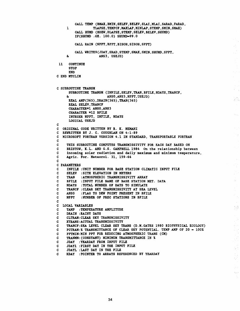
CALL TEMP (BMAX,BMIN,SELEV,BELEV,SLAI,MLAI,SARAD,FARAD, 1 TLAPSE,TEMPCF,MAXLAP,MINLAP,STEHP,SMIN,SMAX)

CALL HUMD (BDEW,DLAPSE,STEMP,SELEV,BELEV,SHUMD) IF(SHUMD .GE. 100.0) SHUMD-99.0

CALL RAIN (NPPT,BPPT,BISOH,SISOH,SPPT)

CALL WRITE9(JDAY,SRAD,STEMP,SMAX,SMIN,SHUMD,SPPT, & ANS3, USEJD)

11 CONTINUE STOP END

C END HTCLIH

C SUBROUTINE TRANSM

c

SUBROUTINE TRANSM (INFILE,SELEV,TRAN,BFILE,NDAYS,TRANCF, & ANSO,ANS3,NPPT,USEJD)

REAL AMP(365),DRAIN(365),TRAN(365) REAL SELEV,TRANCF CHARACTER*l ANSO,ANS3 CHARACTER *12 BFILE INTEGER NPPT, INFILE, NDAYS LOGICAL USEJD

C ORIGINAL CODE WRITTEN BY R. K. NEHANI C REWRITTEN BY J. C. COUGHLAN ON 4-1-89 C MICROSOFT FORTRAN VERSION 4.1 IN STANDARD, TRANSPORTABLE FORTRAN c C THIS SUBROUTINE COMPUTES TRANSMISSIVITY FOR EACH DAY BASED ON C BRISTOW, K.L. AND G.S. CAMPBELL 1984 On the relationship between C incoming solar radiation and daily maximum and minimum temperature, C Agric. For. Meteorol. 31, 159-66 c C PARAMETERS C INFILE :UNIT NUMBER FOR BASE STATION CLIMATIC INPUT FILE C SELEV :SITE ELEVATION IN METERS C TRAN :ATMOSPHERIC TRANSMISSIVITY ARRAY C BFILE :INPUT FILE NAME OF BASE STATION MET. DATA C NDAYS :TOTAL NUMBER OF DAYS TO SIMULATE C TRANCF :CLEAR SKY TRANSMISSIVITY AT SEA LEVEL C ANSO :FLAG TO DEW POINT PRESENT IN BFILE C NPPT :NUMBER OF PREC STATIONS IN BFILE c C LOCAL VARIABLES C TAMP :TEMPERATURE AMPLITUDE C DRAIN :RAINY DAYS C CLTRAN:CLEAR SKY TRANSMISSIVITY C XTRANS:ACTUAL TRANSMISSIVITY C TRANCF:SEA LEVEL CLEAR SKY TRANS (D.M.GATES 1980 BIOPHYSICAL ECOLOGY) C PCTRAN:% TRANSMITTANCE OF CLEAR SKY POTENTIAL. TEMP AMP OF 20 • 100% C PPTMIN:MIN PPT FOR REDUCING ATMOSPHERIC TRANS (CM) C TRANMN:(CONSTANT) MINIMUM TRANSMITTANCE IN% C JDAY :YEARDAY FROM INPUT FILE C JDAYl :FIRST DAY IN THE INPUT FILE C JDAYL :LAST DAY IN THE FILE C KDAY :POINTER TO ARRAYS REFERENCED BY YEARDAY

34

REAL BPPTA(2), BPPT,BMAX,BMIN,BDEW,BMAXl,BMINl,BPPTl,TAMP REAL DIFF,CLTRAN, PCTRAN,XTRANS REAL PPTMIN, TRANMN INTEGER K,KDAY,JDAY,JDAYl,JDAYL,I,M,J

C CONSTANTS DATA PPTMINI0.2541 DATA TRANMNIO.ll

C BEGIN

c

K•O KDAY•O OPEN(INFILE,FILE•BFILE,STATUS•'OLD') REVIND(INFILE)

READ FOR THE 1ST DAY TO INITIALIZE THE LOOP CALL BREAD(INFILE,JDAY,BMAX,BMIN,BDEV,BPPTA,NPPT,

& ANSO,ANS3,USEJD) IF (NPPT .EQ. 2) THEN

BPPT • (BPPTA(l) + BPPTA(2)) I 2 ELSE

BPPT • BPPTA(l) END IF

C MAKE NOTE OF THE FIRST DAY JDAYl • JDAY

C READ TO OBTAIN TEMP AMPLITUDE DO 12 J•l, NDAYS-1

CALL BREAD(INFILE,KDAY,BMAXl,BMINl,BDEV,BPPTA,NPPT, & ANSO,ANS3,USEJD)

IF (NPPT .EQ. 2) THEN BPPTl • (BPPTA(l) + BPPTA(2)) I 2

ELSE BPPTl • BPPTA(l)

END IF

C COMPUTE AMPLITUDE TAMP • BMAX - ((BMIN + BMIN1)12.)

C RAINY DAY CORRECTIONS" IF (BPPT .GT. PPTMIN) THEN

K•K+l DRAIN(K) • JDAY TAMP • TAMP* 0.75

END IF

C SVITCH THE VALUES FROM J+l DAY TO J AMP(JDAY) • TAMP JDAY • KDAY BMAX • BMAXl BMIN • BMINl BPPT•BPPTl

12 CONTINUE

JDAYL • JDAY

C EXCEPTION FOR THE LAST DAY 121 TAMP • BMAX - BMIN

35

IF (BPPT .GT. PPTHIN) TAMP- TAMP*0.75 AMP(JDAY) -TAMP

C CORRECT AMPL VALUES FOR PRE-RAINY DAYS DO 30 I-l,K

KDAY - DRAIN(!) C CANNOT CORRECT THE 1ST AND 2ND DAY SO SKIP

IF ((KDAY-2) .GE. JDAYl) THEN~

DIFF - AMP(KDAY-2) - AMP(KDAY-1) IF (DIFF.GE.2.0) AMP(KDAY-1)- AMP(KDAY-1) * 0.75

END IF 30 CONTINUE

C COMPUTE CLEAR SKY TRANSMITTANCE AT SITE (GATES 1980) CLTRAN- TRANCF + SELEV * 8.0E-5 CLTRAN - AMINl(CLTRAN,l.O)

C COMPUTE TRANSMISSIVITY FOR EACH DAY (BRISTOW AND CAMPBELL 1984) DO 40 M - JDAYl, JDAYL

PCTRAN - (1 - EXP(-0.003*(AMP(M)**2.4))) XTRANS - CLTRAN * PCTRAN TRAN(M) - AMAXl(XTRANS,TRANMN)

40 CONTINUE

C REWIND FILE 8 TO USE AGAIN REWIND(8) CLOSE (8) RETURN END

C SUBROUTINE RAD c

SUBROUTINE RAD(SLAT,SASPCT,SSLOPE,JDAY,SEHORZ,SWHORZ,TRAN, 1 ALBDO,RADN,ARAD,FLAG,ANSl,ANS2)

INTEGER FLAG REAL SLAT, SASPCT, SSLOPE, SEHORZ, SWHORZ REAL ALBDO, ARAD, RADN REAL DEC(46),SOLCON(12),A(2l),TRAN(365) CHARACTER*! ANS1,ANS2

C VALIDATED TO BUFFO BY JCC ON 4-19-89 C RAD COMPUTES INCIDENT SHORTWAVE RADIATION AND C NET SHORTWAVE RADIATION FOR ANY GIVEN DAY BASED ON SURFACE C CHARACTERISTICS, SUN-EARTH GEOMETRY, TRANSMISSIVITY. c C VARIABLES C SLAT: SITE LATITUDE DEGREES C SASPECT:SITE ASPECT X C SSLOPE:SITE SLOPE X C JDAY: CURRENT YEARDAY C SEHORZ:SITE EAST HORIZON IN DEGREES FROM 0 C SWHORZ:SITE WEST HORI IN DEGREES FROM 0 C TRAN:TRANSMISSIVITY ARRAY X C ALBDO:SITE ALBEDO X C ARAD:ABSORBED RADIATION, W/M2 C RADN:INCIDENT RADIATION W/M2 C FLAG:l MEANS SLOPING TERRAIN, 0 MEANS FLAT SURFACE. C ANSl:THRESHOLD RADIATION OF 70 W/MA2 C ANS2:TOTAL RADIATION IF- TOT KJ/MA/DAY

36

c c c

ELSE DAYLIGHT AVERAGE W/MA2

C ORIGINAL CODE WRITTEN BY R. K. NEKANI C REWRITTEN BY J. C. COUGHLAN ON 4-1-89 C MICROSOFT FORTRAN VERSION 4.1 IN STANDARD, TRANSPORTABLE FORTRAN c C THIS CODE CAN BE OPTIMIZED TO THE POINT WHERE IT COTS TOTAL PROGRAM C EXECUTION TIME TO HALF OF THE PRESENT. REMOVE AS MUCH FROM THE DO C LOOP AS POSSIBLE. THE DO LOOP INCREMENTS 10 MINUTES FOR A 24 HOUR C DAY. SOME CALCULATIONS CAN BE DONE ONCE OUTSIDE THE LOOP I.E. C COS(DSLOPE), AND SAVED IN A VARIABLE TO BE USED IN THE LOOP. WE C HAVE KEPT IT LESS EFFICIENT TO REDUCE COMPLEXITY. EFFICIENT CODE C IS LESS READABLE, USUALLY. ALSO, HAVE HARDWARE SUPPORT FOR MATH C REALLY HELPS TOO, ESP. FOR TRIG. FUNCTIONS. -JCC c c c c c c c c c c c c c c c c c c c c c c c c c c c c c c c c c

LOCAL VARIABLE LIST: SOL •SOLAR CONSTANT DERIVED FROM SOLCON ARRAY AM -oPTICAL AIR MASS FOR ANGLES > 21 DEGREES A -oPTICAL AIR MASS ARRAY FOR ANGLES BETWEEN

0 AND 21 DEGREES ABOVE HORIZON DECL •DECLINATION JDAY •DAY OF YEAR ASP •ASPECT IN DEGREES DSLOP •SLOPE IN DEGREES H •ANGLE OF SON FROM SOLAR NOON TRAN •TRANSMISSIVITY CONSTANT TRAM •TRANSMISSIVITY CORRECTED FOR AIR MASS NNH •CALCULATION INTERVAL IN SECONDS. 600 • 10 MINUTES NC •SECONDS IN ONE DAY (24 HOURS) N •NUMBER OF INTERVALS OF LENGTH NNH IN ONE DAY DT •DIRECT SOLAR PERPENDICULAR TO SON ON THE

OUTSIDE OF ATMOSPHERE FOR INTERVAL (KJ,IM**2) ETF •DIRECT SOLAR ON OUTSIDE OF ATMOSPHERE

PARALLEL TO EARTHS SURFACE FOR INTERVAL GRAD •TOTAL DAILY RADIATION AT GIVEN LOCATION (KJ/M**2) BRAD •DIRECT SOLAR ON EARTHS SURFACE (FLAT) TDIF •TOTAL DAILY DIFFUSE RADIATION DIFRAD-DIFFUSE ON SLOPE FOR INTERVAL DRAD •DIRECT ON SLOPE FOR INTERVAL CZA •COSINE ZENITH ANGLE CBSA •COSINE BEAM SLOPE"ANGLE GLOBF -GLOBAL RADIATION, DETERMINING DIFFUSE DIFFL •DIFFUSE ON FLAT FOR INTERVAL DAYL •DAYLENGTH (HOURS) ALBDO •ALBEDO

" " " "

C LOCAL VARIABLES

c

INTEGER NNH,NC,N,MO,IDEC,NH,K,ML REAL CONV,X,ASP,DLAT,SLOPE,DSLOP,XTRAN,DECL,GRAD,TDIF REAL DAYL2,DH,CZA,H,AM,TRAM,DT,ETF,HRAD,GLOBF,DIFFL,CBSA REAL DRAD,SE,DIFRAD,RADT,AVERAD,DAYL,SOL,TDRAD

C CONSTANTS DATA A/2.90,3.05,3.21,3.39,3.69,3.82,4.07,4.37,4.72,5.12

1,5.60,6.18,6.88,7.77,8.90,10.39,12.44,15.36,19.79,26.96 2,30.00/

DATA DEC/-23.,-22.,-21.,-19.,-17.,-15.,-12.,-9.,-6.,-3., 10. J 3. J 6 .• 9. J 12. J 14. J 17. J 19. J 21. J 22. J 23. J 23.5 J 23.5 J 23. J

37

c

221.5. 2o. ,18. ,16. ,14 .• 12 .• 9 .• 6 .• 3 .• o .. -3 .• -6 .• -9 .• -12. , 3-15.,-17.,-19.,-21.,-22.,-23.,-23.5,-23.5/

DATA SOLCON/1.445,1.431,1.410,1.389,1.368,1.354,1.354 1,1.375,1.403,1.424,1.438,1.445/

C FUNCTIONS C CONVERSION STATEMENT FUNCTION FOR DEGREES TO RADIANS

CONV(X)-X/57.296 c C BEGIN C SET THE SLOPE & ASPECT VALUES DEPENDING ON THE FLAG VALUE

IF (FLAG .GT.O) THEN ASP-conv(SASPCT) SLOPE-SSLOPE

ELSE AS P-O SLOPE-0

END IF

C CONVERT PERCENT SLOPE TO DEGREES and to radians DLAT-conv(SLAT) DSLOP-ATAN(SLOPE/100.)*57.29 DSLOP-conv(DSLOP) XTRAN-TRAN(JDAY) NNH-600 NC-86400 N-IFIX(NCfNNH+1.) DAYL-0. MO-IFIX(JDAY/30.+1.) IF (MO.GT.12)Mo-12

C SOLCON ARRAY IS IN UNITS OF ICW/M**2 SOL-SOLCON(MO) IDEC-IFIX(1.+JDAY/8.) DECL-conv(DEC(IDEC)) GRAD-O. TDIF-0. TDRAD-0. NH-0 DAYL2-0.

C DO LOOP INCREMENTS 10 MINUTES, STOPS AFTER 24 HOURS DO 11 K-1,N

NH-NH+NNH C DETERMINE ANGLE FROM SOLAR NOON

DH-(NH-43200)*.0041667

c c

c c

h-conv(dh) CZA-COS(DECL)*COS((DLAT))*COS((H))+SIN((DECL))

1 *SIN( (DLAT)) IF(CZA.GT. 0.) THEN

DAYLENGTH BASED ON SOLAR ELEVATION ABOVE A FLAT HORIZON DAYL2-DAYL2+(NNH/3600.)

NEXT 6 LINES, DETERMINE OPTICAL AIR MASS AM-1./(CZA+.0000001) IF(AM.GT.2.9) THEN

ML-IFIX(ACOS(CZA)/.0174533)-69 IF(ML.LT.1)ML-1 IF(ML.GT.21)HL-21

38

c

c c c c

c c c c

1 2 3 4 5

AM•A(HL) END IF

TRAH•XTRAN**AM DT•SOL*NNH ETF•CZA*DT HRAD-ETF*TRAM DT-DT*TRAH GLOBF•SQRT(HRAD*ETF) DIFFL-GLOBF*(1.-GLOBF/ETF) CBSA•-SIN(DSLOP)*SIN(ASP)*SIN(H) *COS(DECL)+(-COS(ASP)*SIN(DSLOP) *SIN(DLAT)+COS(DSLOP)*COS(DLAT)) *COS(DECL)*COS(H)+(COS(ASP)*SIN(DSLOP) *COS(DLAT)+COS(DSLOP)*SIN(DLAT)) *SIN(DECL) IF(CBSA.GE.O.) THEN

DRAD-CBSA*DT THE FOLLOWING THREE LINES COMPUTES A TOPOGRAPHIC REDUCTION OF DIRECT RADIATION EHE • EAST HORIZON ELEVATION (DEGREES) WHE • WEST HORIZON ELEVATION (DEGREES) SE-1.57-ACOS(CZA) IF(DH.LT.O.AND.SE.LT.CONV(SEHORZ))DRAD-0. IF(DH.GT.O.AND.SE.LT.CONV(SWHORZ))DRAD-0.

ELSE DRAD-0

END IF

DIFRAD-DIFFL*(COS((DSLOP*.5))**2.) RADT-(DRAD+DIFRAD)/FLOAT(NNH)

THE FOLLOWING PROVIDES A MINIMUM RADIATION THRESHOLD OF 70 W/K**2 (0.1 LY/MIN) FOR DAYLENGTH AND RADIATION SUMMATION.

IF(ANS1.EQ.'Y') THEN IF(RADT.GT.0.07) THEN

DAYL • DAYL + (NNH/3600.) GRAD - GRAD + DRAD + DIFRAD TDIF - TDIF + DIFRAD TDRAD - TDRAD + DRAD

END IF ELSE

DAYL • DAYL + (NNH/3600.) GRAD - GRAD + DRAD + DIFRAD TDIF • TDIF + DIFRAD TDRAD • TDRAD + DRAD

END IF END IF

11 CONTINUE IF(ANS2.EQ.'T') THEN

RADN- GRAD ARAD - RADN * (1- ALBDO)

ELSE AVERAD-(GRAD/(DAYL*3600.))

C CONVERT KW/M**2 to W/M**2 RADN - AVERAD * 1000.0 ARAD - RADN * (1-ALBDO)

END IF RETURN

39

END

C SUBROUTINE TEMP c

SUBROUTINE TEMP (BMAX,BHIN,SELEV,BELEV,SLAI,HLAI,SARAD, 1 FARAD,TLAPSE,TEMPCF,MAXLAP,MINLAP,STEMP,SHIN,SMAX)

REAL BMAX, BHIN, SELEV, BELEV, SLAI, HLAI, SARAD, TEMPCF REAL FARAD, TLAPSE, MAXLAP, HINLAP,STEMP, SHIN, SMAX

c c c c c

TEMP COMPUTES SITE DAYLIGHT AVERAGE TEMPERATURE, AND SITE MAX & MIN TEMPS BASED ON BASE STATION DATA AND THEN CORRECTS IT FOR ELEVATION, SLOPE AND ASPECT.

C PARAMETER LIST C BMAX :BASE STATION MAX TEMP C BHIN :BASE STATION MIN TEMP C SELEV :SITE ELEVATION IN METERS C BELEV :BASE ELEVATION IN METERS C SLAI :SITE LAI (ALL SIDES) C HLAI :MAXIMUM LAI (ALL SIDES) FOR HTCLIH ALGORITHMS C SARAD :SITE RADIATION KJ/K"2/DAY C FARAD :FLAT SURFACE RADIATION AT SITE KJ/H"2/DAY C TLAPSE :LAPSE RATE FOR DAYLIGHT AVE TEMP C/1000H C TEMPCF :CONSTANT FOR DAYLIGHT AVE. TEMP (RUNNING ET.AL. C MAXLAP :LAPSE RATE FOR MAX TEMPS C/1000H C HINLAP :LAPSE RATE FOR MIN TEMPS C/1000H C STEMP :SITE DAYLIGHT AVE TEMP C C SHIN :SITE MIN TEMP C C SMAX :SITE MAX TEMP C c C LOCAL VARIABLE LIST C MLAPSE: LAPSE RATE FOR NIGHT MIN TEMPERATURES C DAYLT: DAYLIGHT AVERAGE TEMPERATURE C TSYNOP: SYNOPTIC TEMPERATURE AT THE SITE C RADRAT: RATIO OF FLAT AND SLOPE RADIATION C TADD TEMPERATURE INCREMENT FOR SOUTH SLOPES C TSUB : TEMPERATURE DECREMENT FOR NORTH SLOPES C MLAI : MAXIMUM LAI (ALL SIDES)

C LOCAL VARIABLES REAL LAI, THEAN REAL DAYLT,DELEV,TSYNOP,RADRAT,TSUB,TADD

C IF SITE LAI > MAX LAI THEN USE MAX LAI IN EQUATIONS BELOW IF (SLAI .GT. HLAI) THEN

LAI • HLAI ELSE

LAI • SLAI END IF

C COMPUTE DAYLIGHT AVERAGE TEMP THEAN• (BMAX+BHIN)/2.0 DAYLT• ((BHAX-THEAN)*TEMPCF) + THEAN

C CORRECT FOR LAPSE RATE DELEV • SELEV-BELEV TSYNOP • DAYLT - TLAPSE * (DELEV / 1000.0) SHIN • BHIN - (DELEV/1000.0 * HINLAP)

40

EQ. 1)

SMAX - BMAX - (DELEV/1000.0 * MAXLAP)

C COMPUTE THE RATIO OF SLOPE AND FLAT RADIATION RADRAT - SARAD/FARAD

C ADJUST SYNOPTIC TEMP TO OBTAIN SLOPE TEMP C ADDITIONS MADE ON 10/88 TO ADJUST MAX TEMPS TO RADIATION. C NOT VALIDATED BY LITERATURE. C NOT ADJUSTING MINIMUM TEMPERATURE BECAUSE LONGWAVE NIGHT ADJUSTMENT.

IF (RADRAT.LT.1.0) THEN TSUB-((1/RADRAT)*(1+(LAI/MLAI))) STEHP - TSYNOP - TSUB SMAX - SMAX - TSUB

ELSE TADD-(RADRAT* (1- (LAI/MLAI))) STEMP - TSYNOP + TADD SMAX - SMAX + TADD

END IF RETURN END

SUBROUTINE HUMD (BDEW,DLAPSE,STEMP,SELEV,BELEV,SHUMD) REAL BDEW, DLAPSE,STEMP,SELEV,BELEV,SHUMD

C PARAMETERS C BDEW :BASE STATION BEW POINT C C DLAPSE :DEW POINT LAPSE RATE C STEMP :DAYLIGHT AVE. TEMP. LAPSE RATE C SELEV :SITE ELEVATION IN METERS C BELEV :BASE ELEVATION IN METERS C SHUMD :SITE HUMIDITY % C HUMD COMPOTES RELATIVE HUMIDITY BASED ON BASED C ON BASE STATION DEW POINT c C LOCAL VARIABLES C SDEW :SITE DEW POINT C C ES :AMBIENT VAPOR DENSITY C ESD :SATURATED VAPOR DENSITY

REAL SDEW,ES,ESD

C CORRECT DEW PNT FOR LAPSE SDEW- BDEW - (DLAPSE * ((SELEV-BELEV)/1000.))

C COMPUTE RELATIVE HUMIDITY ES- 6.1078 * EXP((17.269*SDEW)/(237.3 + SDEW)) ESD- 6.1078 * EXP((17.269 * STEMP)/(237.3 + STEHP)) SHUMD-(ES/ESD) * 100.0 RETURN END

SUBROUTINE RAIN (NPPT,BPPT,BISOH,SISOH,SPPT) INTEGER NPPT REAL BISOH(2),SISOH,SPPT,BPPT(2) REAL RAT1, RAT2

C NPPT: NUMBER OF BASE PPT STATIONS

41

C THIS SUBROUTINE COMPUTES SITE PRECIPITATION BY MULTIPLYING C THE BASE STATION PRECIP WITH THE RATIO OF BASE AND SITE C ISOHYETS.

C COMPUTE RATIO OF THE ISOHYTE(S) RAT1 • SISOH/BISOH(1) IF (NPPT .EQ. 2) THEN

RAT2 • SISOH/BISOH(2) SPPT • ( BPPT(1)*RAT1 + BPPT(2)*RAT2 ) / 2.0

ELSE SPPT • RAT1*BPPT(1)

END IF RETURN END

SUBROUTINE HONDAY(JDAY,HON,DAY) INTEGER JDAY,MON,DAY INTEGER DAYS(12) DATA DAYS/31,28,31,30,31,30,31,31,30,31,30,31/ DAY•JDAY HON • 1

10 IF(DAY .GT. DAYS(MON) ) THEN DAY•DAY-DAYS(HON) MON • HON+1 GO TO 10

END IF RETURN END

REAL FUNCTION YEARDAY(HON,IDATE) INTEGER DAYS(12), I,JDAY,MON DATA DAYS/31,28,31,30,31,30,31,31,30,31,30,31/ JDAY • 0 DO 10 I • 1, (HON~1)

JDAY• JDAY+DAYS(I) 10 CONTINUE

JDAY-JDAY+IDATE YEARDAY•JDAY RETURN END

SUBROUTINE WRITE9(JDAY,SRAD,STEMP,SHAX,SHIN,SHUHD,SPPT, & ANS3, USEJD)

INTEGER JDAY,DAY,MON REAL SRAD,STEMP,SMAX,SHIN,SHUMD,SPPT,C2F,X LOGICAL USEJD CHARACTER*1 ANS3

C DEGREE C TO DEGREE F C2F(X) • X *1.8+32.0

IF (ANS3 .EQ. 'E') THEN c CONVERT TEMPERATURES TO DEG F IF INDICATED

STEHP • C2F(STEHP) SHIN • C2F(SMIN) SHAX • C2F(SHAX) SPPT • SPPT/2.54

END IF

42

IF (USEJD) THEN WRITE(9,ll0) JDAY,SRAD,STEMP,SMAX,SMIN,SHUMD,SPPT

110 FORMAT(lX,I3,2X,F8.2,4(F6.0),F5.2) ELSE

CALL MONDAY(JDAY,MON,DAY) WRITE(9,lll) MON,DAY,SRAD,STEMP,SMAX,SMIN,SHUMD,SPPT

lll FORMAT(lX,I2,2X,I3,2X,F8.2, 4(F6.0),F5.2) END IF RETURN END

SUBROUTINE INIT9(IFILE,ANS2,ANS3,USEJD) CHARACTER*l ANS2,ANS3 CHARACTER*80 LINEl, LINE3 CHARACTER*l7 LINE2 CHARACTER*l2 !FILE LOGICAL USEJD

C IDENTIFY THE OUTPUT FILE WRITE(9,*)' MTCLIM OUTPUT FILE' WRITE(9,*)' A LISTING OF INITIALIZATION FILE FOLLOWED BY OUTPUT:' WRITE(9,*)

C LIST INITIALIZATION FILE IN OUTPUT FILE OPEN(UNIT•7,FILE•IFILE)

2 READ(7,l,END-l0) LINEl l FORMAT(lA80)

WRITE(9,l)LINEl GO TO 2

10 CONTINUE WRITE(9,*)

C SET UP HEADINGS FOR OUTPUT FILE IF (USEJD) THEN

LINEl•'JDAY RADIATION STEMP MAXT MINT RH PPT' ELSE

LINEl•'MON DAY RADIATION STEMP MAXT MINT RH PPT' END IF

IF (ANS2 .EQ. 'T') THEN LINE2• ' KJ /M**2 '

ELSE LINE2• ' W /M**2 '

END IF

IF (ANS3 .EQ. 'E') THEN LINE3•LINE2//'F F

ELSE LINE3•LINE2//'C C

END IF

WRITE(9,lll)LINEl,LINE3 111 FORMAT(1A80)

RETURN END

F

c

C SUBROUTINE BREAD: READ BASE STATION DATA.

43

INCHES'

CM '

SUBROUTINE BREAD(INFILE,JDAY,BMAX,BMIN,BDEV,BPPT,NPPT, & ANSO,ANS3,USEJD)

INTEGER INFILE, JDAY, NPPT REAL BMAX,BMIN REAL BPPT(2) CHARACTER*1 ANSO, ANS3 LOGICAL USEJD

C VARIABLES C INFILE: INTEGER UNIT NUMBER OF BASE STATION CLIMATIC INPUT FILE C JDAY: YEARDAY C BHAX: MAXIMUM TEMPERATURE C BMIN: MINIMUM TEMPERATURE C BDEW: DEW POINT TEMPERATURE C NPPT: NUMBER OF BASE STATIONS 1 OR 2 C ANSO: IS DEW POINT SUPPLIED IN FILE C IF NOT THEN SET IT TO NIGHT MINIMUM TEMPERATURE. C ANS3: IS INPUT IN ENGLISH OR SI UNITS, 'E' - ENGLISH SO CONVERT TO SI c C FUNCTION F2C: DEGREE F TO DEGREE C

REAL F2C,X,YEARDAY INTEGER DAY, MON F2C(X) - (X-32)*0.5556

C BEGIN IF (USEJD) THEN

IF(ANSO.EQ.'Y') THEN IF(NPPT .EQ. 1) THEN

READ(INFILE,*) JDAY, BMAX, BMIN, BDEW, BPPT(1) BPPT(2) - 0.0

ELSE READ(S,*) JDAY, BMAX, BMIN, BDEW, BPPT(1), BPPT(2)

END IF ELSE

IF(NPPT .EQ. 1) THEN READ(INFILE,*) JDAY, BMAX, BMIN, BPPT(1) BPPT(2) - 0.0 BDEW-BMIN

ELSE READ(INFILE,*) JDAY, BMAX, BMIN, BPPT(1), BPPT(2) BDEW - BMIN

END IF END IF

ELSE IF(ANSO.EQ.'Y') THEN

IF(NPPT .EQ. 1) THEN READ(INFILE,*) MON,DAY, BHAX, BMIN, BDEW, BPPT(1) BPPT(2) - 0.0

ELSE READ(S,*) MON,DAY, BHAX, BMIN, BDEW, BPPT(1), BPPT(2)

END IF ELSE

IF(NPPT .EQ. 1) THEN READ(INFILE,*) MON,DAY, BMAX, BMIN, BPPT(1) BPPT(2) - 0.0 BDEW-BMIN

ELSE READ(INFILE,*) MON,DAY, BMAX, BMIN, BPPT(1), BPPT(2) BDEW - BMIN

END IF END IF

44

JDAY•YEARDAY(HON,DAY) END IF

IF (ANS3 .EQ. 'E') THEN C CONVERT ENGLISH UNITS TO SI

BPPT(l) - BPPT(l) * 2.54 BPPT(2) - BPPT(2) * 2.54 BMAX - F2C(BHAX)

c

BHIN - F2C(BHIN) BDEW • F2C(BDEW)

END IF

RETURN END

C ---------------- END LISTING -----------------

45

APPENDIX B: SINE FORM FOR AVERAGING TEMPERATURE

The assumption that daylight average temperature is described by three quadrants of the sine function is illustrated in figure 12. Minimum temperature usually occurs at or close to sunrise, maximum temperature occurs near midday, and temperature at sunset is somewhere in between maximum and minimum. Using this assumption and integrating the area under the curve the value for TEMCF is 0.212.

To test if the sine form weighted air temperature (T ) is a more accurate measure ave of daylight air temperature than the normally used arithmetic mean average air tem-perature (Tmean), 120 days ofhourly measured meteorological data from Fraser Experi­mental Forest, Colorado, were used as a benchmark. Regressions of the Tave and T mean data against the hourly averaged daylight air temperatures were calculated and found to be:

Tha = -1.14 + 1.12 Tave r = 0.93; and:

n = 120 days

Th = 0.74 + 1.20 T r = 0.88; n = 120 days a mean

where:

T ha = daylight air temperature, hourly averaged.

The sine form weighted average more closely approximated the benchmark hourly averaged daylight air temperature as evidenced by a higher correlation coefficient and a slope closer to 1.0.

Observation of diurnal temperature traces for sites at Coram and other locations in the Northern Rocky Mountains indicate that temperature rises more rapidly after sunrise than given by the sine function (fig. 12). The maximum temperature may be shifted to the left, and the peak widened (fig. 12). Actual sunset is at 3rr/4, thus the daylight period is shorter than assumed by the sine function (fig. 12). The net result is that the average daylight temperatures are greater than estimated by the sine func­tion and TEMCF is greater (0.45) as shown in figure 12 for an observed data set.

Observed daylight average data (based on hourly readings) for several sites (Lubrecht, Coram 12, 14, 33, and 23) were used to calculate TEMCF. Two procedures were used. The first substituted observed daily average values into equation 1, then solved for TEMCF. The second used a regression procedure with the observed daily average values to provide a least squares estimate for TEMCF. When data for a whole season were used, calculated values ranged from 0.30 to 0.60. Values for these analyses averaged close to 0.45 for TEMCF; thus, this value was used in our model analyses to compare predicted with observed daylight average temperatures.

-1

OBSERVED

(MAXIMUM TAIR)

(MINIMUM RH)

46

ACTUAL SUNSET

SINE FUNCTION

Figure 12-The sine wave used to approximate daylight average temperature and the observed pattern of tempera­ture amplitude.

APPENDIX C: ESTIMATING DAILY DEWPOINT TEMPERATURE

Comparison of spatial differences in dewpoint are made for two locations in western Montana that are 100 miles apart (fig. 13). There appears to be a good relationship with the slope of the regression line very close to 1.0 and the intercept near 0.0, with most points fairly close to the line.

The assumption that dewpoint is equal to night minimum temperature is tested us­ing two data sets in western Montana. Results of regression analyses for data at Lubrecht in 1984 are shown in figure 14. The relationship is quite good, with an r 2 of 0.85. The figure does show that for some days during the summer dewpoint tempera­ture can be much less than night minimum. Results from the Missoula NWS data were nearly identical (r2 = 0.88, slope = 0.88, and intercept= 0.4 7) to the results from Lubrecht. Although errors can occur for individual days, the relationship is strong enough that night minimum temperature is a reasonable estimator of dewpoint temperature.

y = -0.62 + 1.03X R2 = 0.88

(.) 10.0 ••• 0

..A-

..J 11.1 • 0.. • en • :::; ~ • ~ • I

1- 0.0 z • 0 • c. • ~ •• Figure 13-The relationship be-LIJ c tween dewpoint measured at

the Missoula, MT, airport and • the Kalispell, MT, airport 120 •

miles away, for 204 days from -10.0 o.o 10.0 April-November 1983, as a test

DEWPOINT- MISSOULA, °C of regional equivalence of daily absolute humidity.

10

6

6 0

0

u.i 4 a:: ::l 1-cl: 2 a: w 0.. :i w 0 1-...

-2 z 0 0..

~ -4 w Figure 14-The relationship between 0

-6 dewpoint and night minimum air tern-perature found for the period Year Day

-a 65-299, 1984, at Lubrecht Experimen-tal Forest in western Montana. This

-10 • test was done to determine how accu-

-5 -3 -1 3 5 7 9 11 13 rately dewpoint can be estimated from night minimum temperature if humidity

NIGHT MINIMUM AIR TEMP, °C data is not available.

47

Equations for Calculating Atmospheric Transmissivity

Equations for Calculating Potential Incoming Radiation

APPENDIX D: EQUATIONS FOR CALCULATING SOLAR RADIATION

The equations for calculating atmospheric transmissivity in MTCLIM are a modification of the equations from Bristow and Campbell, 1984. The equations are used to calculate a multiplier that is used for calculating incoming solar radiation.

The equation used to calculate maximum clear sky atmospheric transmittance corrected for elevation is:

A = TRANCF + (SELEV) (0.00008) (1)

where A is the maximum clear sky atmospheric transmittance of the study area or region, TRANCF is the clear sky transmittance of the site equivalent to sea level (assumed to be 0.65 for western Montana), and SELEV is elevation of the site in meters. The value 0.00008 is the correction for increasing transmittance with in­creases in elevation.

Clear sky transmittance (A) is used to calculate atmospheric transmittance as a function of daily air temperature range by the equation from Bristow and Campbell (1984):

Tt = A(1~xp(-B~TC)) (2)

where Tt is the daily total atmospheric transmittance, A is the maximum clear sky transmittance from equation (1), ~Tis the daily range of air temperature, and B and C are empirical coefficients that determine how soon maximum Tt is achieved as ~T increases. In MTCLIM B = -0.0030 and C = 2.4, based on conditions for western Montana and northern Idaho. Bristow and Campbell discuss methods for determining the value forB and C. In their paper, B changed with season (0.004 in summer and 0.010 in winter) and C was held constant at 2.4.

The daily range of air temperature (~T) is calculated by the equation:

~Ti = T maxi- (T mini+ T mifli + 1)/2 (3)

where ~T. is the daily range of temperature for thejth day, T . is the maximum temperat~re on the jth day, T . . is the minimum temperatur~n the jth day, and T .. +1 is the minimum temp;:ture on the day following thejth day. Once ~T. is c:l~itlated from equation (3), it is corrected for rainy periods. If it rained on the'jth day ~T. from equation (3) was corrected, making ~T = 0.75 ~T .. If ~T. 1 was less than i.T. 2 by more than 2 oc, ~T.

1 = 0.75 ~T. 1• In this situdtion it is assumed

that the Jc1oudy conditions began ~n day j-1, r~sulting in a large drop in incoming radiation. See Bristow and Campbell, 1984 for more details.

The equations used to calculate potential incoming radiation are based on Gamier and Ohmura (1968), Buffo and others (1972), and Swift (1976). The basic equation calculates incoming radiation on the slope:

~=~+~ w where Q is the total incoming radiation on a slope (kJ/m2) at the earth's surface, Is is th: direct beam radiation on a slope at the earth's surface, and D is the dif-fu~e radiation at the surface.

8

The direct beam radiation Is at the surface is calculated by: s

Is = cos<I>(R N *TtAM) (5) s 0

where R is the solar constant (kW/m2) above the atmosphere, with an average value fo; each month; N is the time interval for calculation in seconds; Tt is the daily total transmittance from equation (2); and AM is the optical air mass calculated by

AM= 1.0/cose + 1.0 x 10-7 (6)

48

Notation

where cos9 is the cosine of the zenith angle (CZA in the code in appendix A) calculated by equation (11). If AM is >2.9 then:

ML = IFIX(Amcos(cos0)/0.0174533)- 69 (7)

where IFIX converts a real value into an integer, A is the optical air mass value in m an array (data values are in code in appendix A) for angles between 0 and 21 de-grees above the horizon. If ML is <1, ML is set equal to 1.0; if ML is >21, ML is set equal to 21, then AM is equal to A * ML. m

Coscp (CBSA in the code in appendix A) is the cosine of the beam slope angle and is given by

coscp = -sinS*sinAZ*sinH*cos8 + (-cosAZ*sinS*sinL+cosS*cosL)* (8) cosO*cosH + (cosAZ*sinS*cosL + cosS*sinL)*sino

where S is the slope in degrees, AZ is aspect in degrees, H is hour angle calculated by H = (NH- 43200)*0.0041667 (NH is time of day), o is declination of the sun based on time of year (values are given in code in appendix A for 8-day periods through the year as the variable DEC), and L is latitude in degrees.

The diffuse radiation at the surface on a slope is calculated by:

Ds = n, *COs(S/2)2 (9)

where D f is the diffuse radiation on a flat surface, and S is the slope in degrees.

D = ((cos9R N)2TAM)0·5*(1-cos9R NTAM)0·5 (10) f 0 t 0 t

where R0

, N, T1, and AM have been defined for equations 2, 5, 6, and 7. Cos9 is the cosine of the zenith angle (CZA in the code in appendix A) of the sun given by:

cos9 = cosO*COsL*cosH + sino*sinL (11)

where o, L, and H are as defined for equation 8.

The above equations calculate total radiation or average radiation from sunrise to sunset.

Qs

I sf Is s n, D s coscp

Total incoming radiation on a sloping surface (GRAD in appendix A)

Direct beam radiation on a flat surface (HRAD in appendix A) Direct beam radiation on a sloping surface (DRAD in appendix A)

Diffuse radiation on a flat surface (DIFFL in appendix A)

Diffuse radiation on a sloping surface (DIFRAD in appendix A)

cosine beam slope angle (CBSA in appendix A) cos9 cosine zenith sun angle (CZA in appendix A)

o declination angle of sun (DECL in appendix A) L latitude of site in degrees (SLAT in appendix A)

H hour angle of sun from solar noon (H in appendix A) AZ aspect of site in degrees (SASPCT in appendix A)

S slope in degrees (SSLOPE in appendix A) R solar constant (SOLCON in appendix A)

0

Tt atmospheric transmissivity constant (TRAN in appendix A) AM optical air mass (AM in appendix A)

A maximum clear sky atmospheric transmittance B empirical coefficient (--0.0030 in MTCLIM)

C empirical coefficient (2.4 in MTCLIM)

TRANCF clear sky transmittance equivalent to sea level

SELEV elevation of site in meters

49

T air temperature llT daily range of air temperature

T max maximum temperature for a day T . minimum temperature for a day

mm

N time interval

APPENDIX E: CALCULATING HORIZON ANGLES FROM A TOPOGRAPHIC MAP

The angles to the east and west horizons, if they have not been measured, can be calculated using a topographic map. These angles are used in MTCLIM to truncate direct-beam incoming radiation at sunrise and sunset to account for blockage of the sun by ridges, tree lines, or other obstacles that block the sun. Figure 15 is a simple diagram of an elevation view of a site on a flat with ridges to the east and west. The angle e in degrees needs to be calculated and entered in the INIT.DAT file as EAST-HORIZ and WEST-HORIZ. The angle e is calculated using the following relation

e = arctan hid (1)

where h is the elevation difference (feet) between the site and the ridge top blocking the sun, and dis the horizontal distance (feet) from the site to the ridge top blocking the sun. The elevation difference h is obtained from a topographic map by calculat­ing the difference in elevation, given by the contours, between the ridge, or other obstacle, and the site. The horizontal distanced is a straight-line distance on the map between the site and ridge top, converted to feet using the appropriate scale for the map.

, ,' , , , ,

, , , , ,

, , , , , " ,

Figure 15-Measurements needed to calculate east and west horizon angles from a topographic map.

50

APPENDIX F: EQUATIONS FOR CALCULATING PRECIPTATION

The equations used to calculate daily precipitation at the site are based on daily precipitation at one base station, or two base stations if data are available. The equation using one base station is

ps = PBl*As/AB (1)

and the equation using two base stations is

ps = (P Bl * A/ABl + p B2 * A/AB2) 12 (2)

where P is daily precipitation at the site, P Bl is daily precipitation input from the first

8(or only) base station, P B2 is daily precipitation input from the second base

station, A is the long-term average annual precipitation at the site (from a precipi­tation map), and ABl and AB2 are average annual precipitation from the first and second base stations.

51

APPENDIX G: EQUATIONS FOR CALCULATING HUMIDITY

The equations used to calculate day average relative humidity are based on dew­point at the base station, which is corrected for elevation to the site, and day aver­age temperature at the site calculated by MTCLIM using the equations given on page 4. The equations are based on Murray (1967) and are given by

SRH= (ESIESD)*100

where SRH is day average site relative humidity in percent andES is the satura­tion vapor pressure at dewpoint given by

ES = 6.1078*e<17.269..SDEWV(237.a +SDEW)

and ESD is the saturation vapor pressure at the day average temperature given by ESD = 6.1078*e<17.269..STEMP)I(237.a +STEMP>

STEMP is the day average temperature at the site calculated by MTCLIM and SDEW is the dewpoint at the site given by

SDEW = BDEW- DLAPSE * (SELEV-BELEV)/1,000

where BDEW is the dewpoint at the base station, DLAPSE is the lapse rate for humidity (1.5 °F per 1,000 ft or 2. 7 °C/1,000 m elevation), SELEV is the elevation in meters at the site, and BELEV is the elevation of the base station. When BDEW is not available or used the minimum temperature for the day is set equal to the dewpoint (appendix C).

52

Hungerford, Roger D.; Nemani, Ramakrishna R.; Running, Steven W.; Coughlan, Joseph C. 1989. MTCLIM: a mountain microclimate simulation model. Res. Pap. INT-414. Ogden, UT: U.S. Department of Agriculture, Forest Service, Intermountain Research Station. 52 p.

A model for calculating daily microclimate conditions in mountainous terrain is presented. Daily air temperature, shortwave radiation, relative humidity, and precipitation are extrapolated form data measured at National Weather Service stations. The model equations are given and the paper describes how to execute the model. Model outputs are compared with observed data from several mountain sites.

KEYWORDS: meterology, weather, climatology, temperature, solar radiation, humidity, precipitation, model

INTERMOUNTAIN RESEARCH STATION

The Intermountain Research Station provides scientific knowledge and technology to im­prove management, protection, and use of the forests and rangelands of the Intermountain West. Research is designed to meet the needs of National Forest managers, Federal and State agencies, industry, academic institutions, public and private organizations, and indi­viduals. Results of research are made available through publications, symposia, workshops, training sessions, and personal contacts.

The Intermountain Research Station territory includes Montana, Idaho, Utah, Nevada, and western Wyoming. Eighty-five percent of the lands in the Station area, about 231 million acres, are classified as forest or rangeland. They include grasslands, deserts, shrublands, alpine areas, and forests. They provide fiber for forest industries, minerals and fossil fuels for energy and industrial development, water for domestic and industrial con­sumption, forage for livestock and wildlife, and recreation opportunities for millions of visitors.

Several Station units conduct research in additional western States, or have missions that are national or international in scope.

Station laboratories are located in:

Boise, Idaho

Bozeman, Montana (in cooperation with Montana State University)

Logan, Utah (in cooperation with Utah State University)

Missoula, Montana (in cooperation with the University of Montana)

Moscow, Idaho (in cooperation with the University of Idaho)

Ogden, Utah

Provo, Utah (in cooperation with Brigham Young University)

Reno, Nevada (in cooperation with the University of Nevada)

USDA policy prohibits discrimination because of race, color, national origin, sex, age, reli­gion, or handicapping condition. Any person who believes he or she has been discriminated against in any USDA-related activity should immediately contact the Secretary of Agriculture, Washington, DC 20250.