multi-armed bandit: learning in dynamic systems with ...ewh.ieee.org/r10/xian/com/zhaoqing.pdfc...
TRANSCRIPT

c©Qing Zhao, UC Davis. Talk at Xidian Univ., September, 2011. 1
Multi-Armed Bandit:
Learning in Dynamic Systems with Unknown Models
Qing Zhao
Department of Electrical and Computer Engineering
University of California, Davis, CA 95616
Supported by NSF, ARL, ARO.

c©Qing Zhao, UC Davis. Talk at Xidian Univ., September, 2011. 2
Clinical Trial (Thompson’33)
Two treatments with unknown effectiveness:

c©Qing Zhao, UC Davis. Talk at Xidian Univ., September, 2011. 3
Applications of MAB
Web Search Internet Advertising
Queueing and Scheduling
λ1
λ2
Multi-Agent Systems

c©Qing Zhao, UC Davis. Talk at Xidian Univ., September, 2011. 4
Multi-Armed Bandit
Multi-Armed Bandit:
◮ N arms and a single player.
◮ Select one arm to play at each time.
◮ i.i.d. reward with Unknown mean θi.
◮ Maximize the long-run reward.
c©Qing Zhao, UC Davis. Talk at Xidian Univ., September, 2011. 5
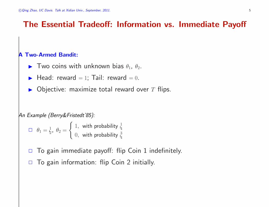
The Essential Tradeoff: Information vs. Immediate Payoff
A Two-Armed Bandit:
◮ Two coins with unknown bias θ1, θ2.
◮ Head: reward = 1; Tail: reward = 0.
◮ Objective: maximize total reward over T flips.
An Example (Berry&Fristedt’85):
2 θ1 =12, θ2 =
{
1, with probability 14
0, with probability 34
2 To gain immediate payoff: flip Coin 1 indefinitely.
2 To gain information: flip Coin 2 initially.

c©Qing Zhao, UC Davis. Talk at Xidian Univ., September, 2011. 6
Two Formulations
Bayesian Formulation:
◮ {θi} are random variables with prior distributions {fθi}.
◮ Policy π: choose an arm based on {fθi} and the observation history.
◮ Objective: policies with good average (over {fθi}) performance.
c©Qing Zhao, UC Davis. Talk at Xidian Univ., September, 2011. 7
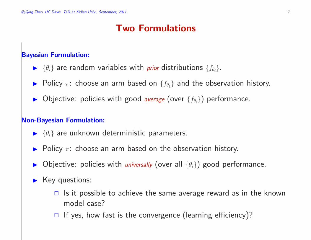
Two Formulations
Bayesian Formulation:
◮ {θi} are random variables with prior distributions {fθi}.
◮ Policy π: choose an arm based on {fθ1} and the observation history.
◮ Objective: policies with good average (over {fθi}) performance.
Non-Bayesian Formulation:
◮ {θi} are unknown deterministic parameters.
◮ Policy π: choose an arm based on the observation history.
◮ Objective: policies with universally (over all {θi}) good performance.
◮ Key questions:
2 Is it possible to achieve the same average reward as in the known
model case?
2 If yes, how fast is the convergence (learning efficiency)?
c©Qing Zhao, UC Davis. Talk at Xidian Univ., September, 2011. 8
Bayesian Formulation
c©Qing Zhao, UC Davis. Talk at Xidian Univ., September, 2011. 9
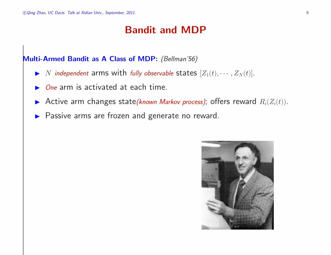
Bandit and MDP
Multi-Armed Bandit as A Class of MDP: (Bellman’56)
◮ N independent arms with fully observable states [Z1(t), · · · , ZN(t)].
◮ One arm is activated at each time.
◮ Active arm changes state(known Markov process); offers reward Ri(Zi(t)).
◮ Passive arms are frozen and generate no reward.
c©Qing Zhao, UC Davis. Talk at Xidian Univ., September, 2011. 10
Bandit and MDP
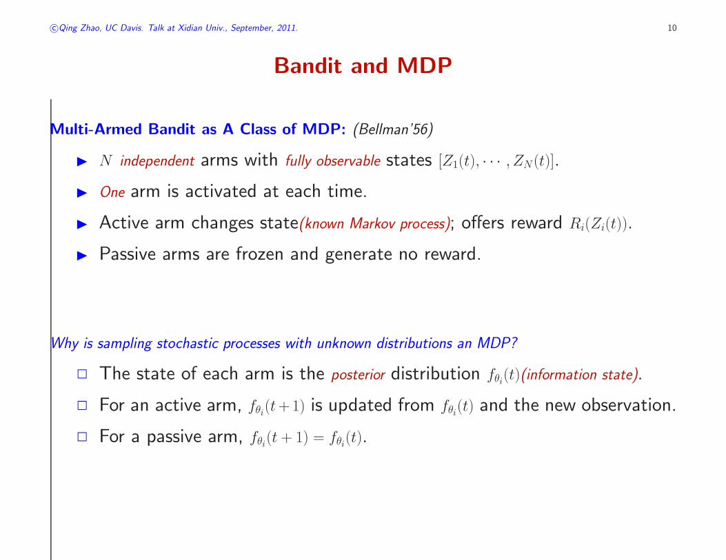
Multi-Armed Bandit as A Class of MDP: (Bellman’56)
◮ N independent arms with fully observable states [Z1(t), · · · , ZN(t)].
◮ One arm is activated at each time.
◮ Active arm changes state(known Markov process); offers reward Ri(Zi(t)).
◮ Passive arms are frozen and generate no reward.
Why is sampling stochastic processes with unknown distributions an MDP?
2 The state of each arm is the posterior distribution fθi(t)(information state).
2 For an active arm, fθi(t+1) is updated from fθi(t) and the new observation.
2 For a passive arm, fθi(t + 1) = fθi(t).

c©Qing Zhao, UC Davis. Talk at Xidian Univ., September, 2011. 11
Bandit and MDP
Multi-Armed Bandit as A Class of MDP: (Bellman’56)
◮ N independent arms with fully observable states [Z1(t), · · · , ZN(t)].
◮ One arm is activated at each time.
◮ Active arm changes state(known Markov process); offers reward Ri(Zi(t)).
◮ Passive arms are frozen and generate no reward.
Solving Multi-Armed Bandit using Dynamic Programming:
◮ Exponential complexity with respect to N .

c©Qing Zhao, UC Davis. Talk at Xidian Univ., September, 2011. 12
Gittins Index
The Index Structure of the Optimal Policy: (Gittins’74)
◮ Assign each state of each arm a priority index.
◮ Activate the arm with highest current index value.
Complexity:
c©Qing Zhao, UC Davis. Talk at Xidian Univ., September, 2011. 13
Gittins Index
The Index Structure of the Optimal Policy: (Gittins’74)
◮ Assign each state of each arm a priority index.
◮ Activate the arm with highest current index value.
Complexity:
◮ Arms are decoupled (1 N-dim to N separate 1-dim problems).
◮ Linear complexity with N .
◮ Polynomial (cubic) with the state space size of a single arm
(Varaiya&Walrand&Buyukkoc’85, Katta&Sethuraman’04).

c©Qing Zhao, UC Davis. Talk at Xidian Univ., September, 2011. 14
Restless Bandit
λ1
λ2

c©Qing Zhao, UC Davis. Talk at Xidian Univ., September, 2011. 15
Restless Bandit
Restless Multi-Armed Bandit: (Whittle’88)
◮ Passive arms also change state and offer reward.
◮ Activate K arms simultaneously.
Structure of the Optimal Policy:
◮ Not yet found.
Complexity:
◮ PSPACE-hard (Papadimitriou&Tsitsiklis’99).
c©Qing Zhao, UC Davis. Talk at Xidian Univ., September, 2011. 16
Whittle Index
Whittle Index: (Whittle’88)
2 Optimal under relaxed constraint on the average number of active arms.
2 Asymptotically (N → ∞) optimal under certain conditions (Weber&Weiss’90).
2 Near optimal performance observed from extensive numerical examples.
Difficulties:
2 Existence (indexability) not guaranteed and difficult to check.
2 Numerical index computation infeasible for infinite state space.
2 Optimality in finite regime difficult to establish.
c©Qing Zhao, UC Davis. Talk at Xidian Univ., September, 2011. 17
Spectrum Opportunity Tracking
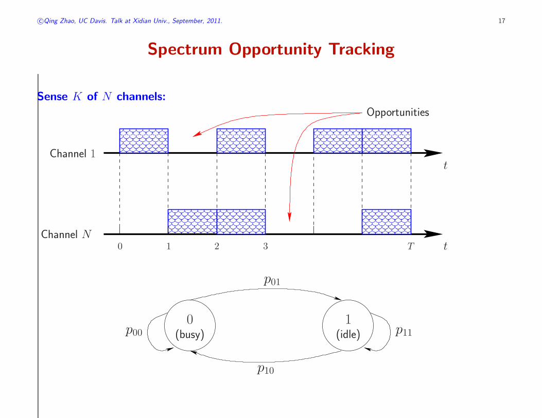
Sense K of N channels:
������������������������������������
������������������������������������
��������������������������������
��������������������������������
������������������������������������
������������������������������������
������������������������������������
������������������������������������
������������������������������������
������������������������������������
��������������������������������
��������������������������������
������������������������������������
������������������������������������
Opportunities
Channel 1
Channel N0 1 2 3 T t
t
0 1(busy) (idle)
p01
p11p00
p10

c©Qing Zhao, UC Davis. Talk at Xidian Univ., September, 2011. 18
Spectrum Opportunity Tracking
������������������������������������
������������������������������������
��������������������������������
��������������������������������
������������������������������������
������������������������������������
������������������������������������
������������������������������������
������������������������������������
������������������������������������
��������������������������������
��������������������������������
������������������������������������
������������������������������������
Opportunities
Channel 1
Channel N0 1 2 3 T t
t
◮ Each channel is considered as an arm.
◮ State of arm i: posterior probability that channel i is idle.
ωi(t) = Pr[channel i is idle in slot t | O(1), · · · , O(t− 1)︸ ︷︷ ︸
observations
]
◮ The expected immediate reward for activating arm i is ωi(t)

c©Qing Zhao, UC Davis. Talk at Xidian Univ., September, 2011. 19
Markovian State Transition
0 1(busy) (idle)
p01
p11p00
p10
◮ If channel i is activated in slot t:
ωi(t + 1) =
{
p11, if Oi(t) = 1
p01, if Oi(t) = 0.
◮ If channel i is made passive in slot t:
ωi(t + 1) = ωi(t)p11 + (1− ωi(t))p01.

c©Qing Zhao, UC Davis. Talk at Xidian Univ., September, 2011. 20
Structure of Whittle Index Policy
The Semi-Universal Structure of Whittle Index Policy:
◮ No need to compute the index.
◮ No need to know {p01, p11} except their order (robust to model mismatch).
p11 ≥ p01 (positive correlation):
������������������������
������������������������
��������������������������������������������������������������������
��������������������������������������������������������������������
��������������������������������������������
��������������������������������������������
p11 < p01 (negative correlation):
������������
������������
������������������������
������������������������
������������������������
������������������������
����������������
����������������
��������������������
��������������������
����������������
����������������
c©Qing Zhao, UC Davis. Talk at Xidian Univ., September, 2011. 21
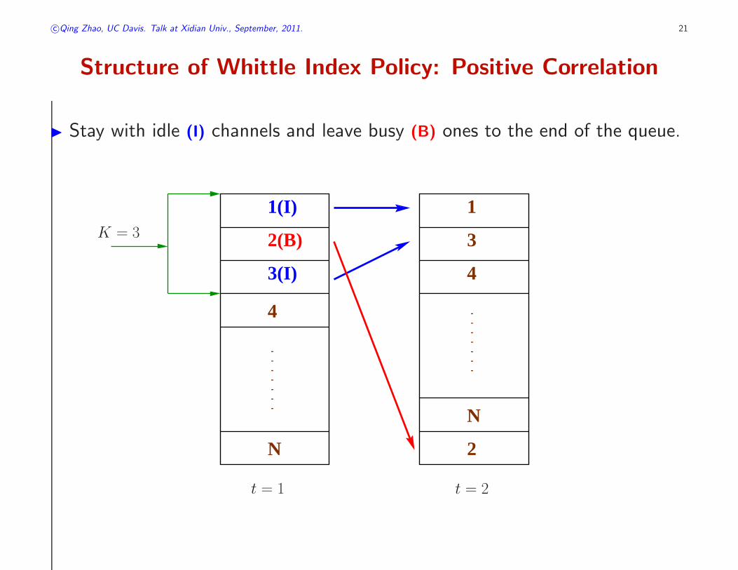
Structure of Whittle Index Policy: Positive Correlation
◮ Stay with idle (I) channels and leave busy (B) ones to the end of the queue.
1(I)
N
2(B)
3(I)
4
2
1
3
4
N
K = 3
t = 1 t = 2

c©Qing Zhao, UC Davis. Talk at Xidian Univ., September, 2011. 22
Structure of Whittle Index Policy: Negative Correlation
◮ Stay with busy (B) channels and leave idle (I) ones to the end of the queue.
◮ Reverse the order of unobserved channels.
reversed
N
2(B)
3(I)
4
3
21(I)
4
1
NK = 3
t = 1 t = 2

c©Qing Zhao, UC Davis. Talk at Xidian Univ., September, 2011. 23
Optimality of Whittle Index Policy
Optimality for positively correlated channels:
◮ holds for general N and K.
◮ holds for both finite and infinite horizon (discounted/average reward).
Optimality for negatively correlated channels:
◮ holds for all N with K = N − 1.
◮ holds for N = 2, 3.
c©Qing Zhao, UC Davis. Talk at Xidian Univ., September, 2011. 24
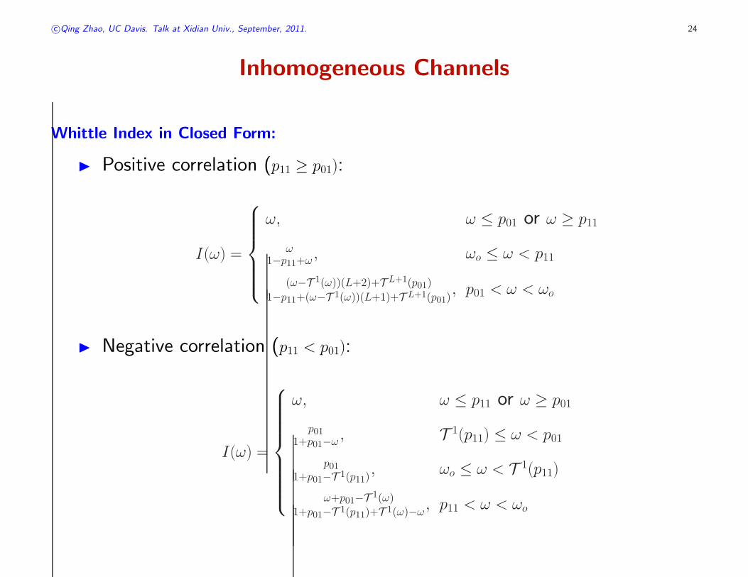
Inhomogeneous Channels
Whittle Index in Closed Form:
◮ Positive correlation (p11 ≥ p01):
I(ω) =
ω, ω ≤ p01 or ω ≥ p11
ω1−p11+ω
, ωo ≤ ω < p11
(ω−T 1(ω))(L+2)+T L+1(p01)
1−p11+(ω−T 1(ω))(L+1)+T L+1(p01), p01 < ω < ωo
◮ Negative correlation (p11 < p01):
I(ω) =
ω, ω ≤ p11 or ω ≥ p01
p011+p01−ω
, T 1(p11) ≤ ω < p01
p011+p01−T 1(p11)
, ωo ≤ ω < T 1(p11)
ω+p01−T 1(ω)1+p01−T 1(p11)+T 1(ω)−ω
, p11 < ω < ωo
c©Qing Zhao, UC Davis. Talk at Xidian Univ., September, 2011. 25
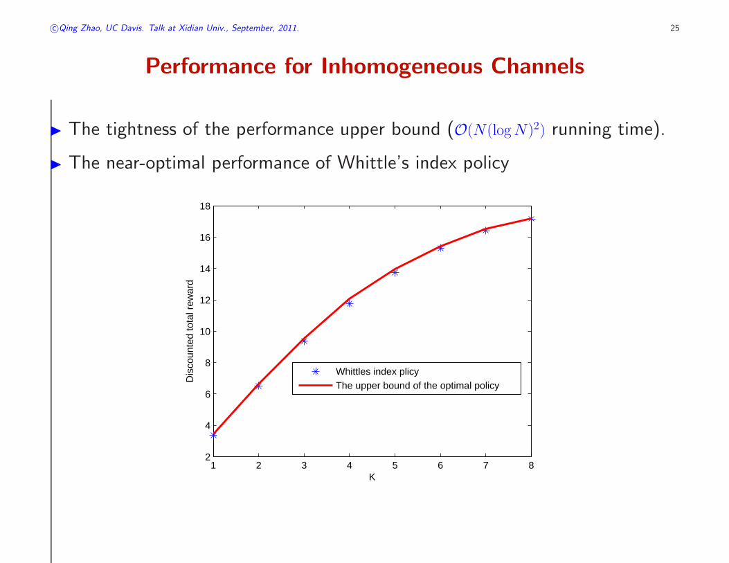
Performance for Inhomogeneous Channels
◮ The tightness of the performance upper bound (O(N(logN)2) running time).
◮ The near-optimal performance of Whittle’s index policy
1 2 3 4 5 6 7 82
4
6
8
10
12
14
16
18
K
Dis
coun
ted
tota
l rew
ard
Whittles index plicyThe upper bound of the optimal policy
c©Qing Zhao, UC Davis. Talk at Xidian Univ., September, 2011. 26
Non-Bayesian Formulation

c©Qing Zhao, UC Davis. Talk at Xidian Univ., September, 2011. 27
Non-Bayesian Formulation
Performance Measure: Regret
◮ Θ∆= (θ1, · · · , θN): unknown reward means.
◮ θ(1)T : max total reward (by time T) if Θ is known.
◮ V πT (Θ): total reward of policy π by time T .
◮ Regret (cost of learning):
RπT (Θ)
∆= θ(1)T − V π
T (Θ) =N∑
i=2
(θ(1) − θ(i))E[time spent on θ(i)].
Objective: minimize the growth rate of RπT (Θ) with T .
sublinear regret =⇒ maximum average reward θ(1)

c©Qing Zhao, UC Davis. Talk at Xidian Univ., September, 2011. 28
Classic Results
◮ Lai&Robbins’85:
R∗T (Θ) ∼
N∑
i=2
θ(1) − θ(i)
I(θ(i), θ(1))︸ ︷︷ ︸
KL divergence
log T as T → ∞.
◮ Agrawal’95, Auer&Cesa-Bianchi&Fischer&Informatik’02:
2 Sample-mean based index policies.
2 UCB policy: index = θ̄i +√
2 log tτi(t)
.

c©Qing Zhao, UC Davis. Talk at Xidian Univ., September, 2011. 29
Classic Results
◮ Lai&Robbins’85:
R∗T (Θ) ∼
N∑
i=2
θ(1) − θ(i)
I(θ(i), θ(1))︸ ︷︷ ︸
KL divergence
log T as T → ∞.
◮ Agrawal’95, Auer&Cesa-Bianchi&Fischer&Informatik’02:
2 Sample-mean based index policies.
2 UCB policy: index = θ̄i +√
2 log tτi(t)
.
◮ Limitations:
2 Reward distributions limited to exponential family or finite support.
2 Assume known distribution type or support range.
2 i.i.d. reward.
2 A single player (equivalently, centralized multiple players).

c©Qing Zhao, UC Davis. Talk at Xidian Univ., September, 2011. 30
General Reward Distributions
c©Qing Zhao, UC Davis. Talk at Xidian Univ., September, 2011. 31
MAB with A General Reward Model
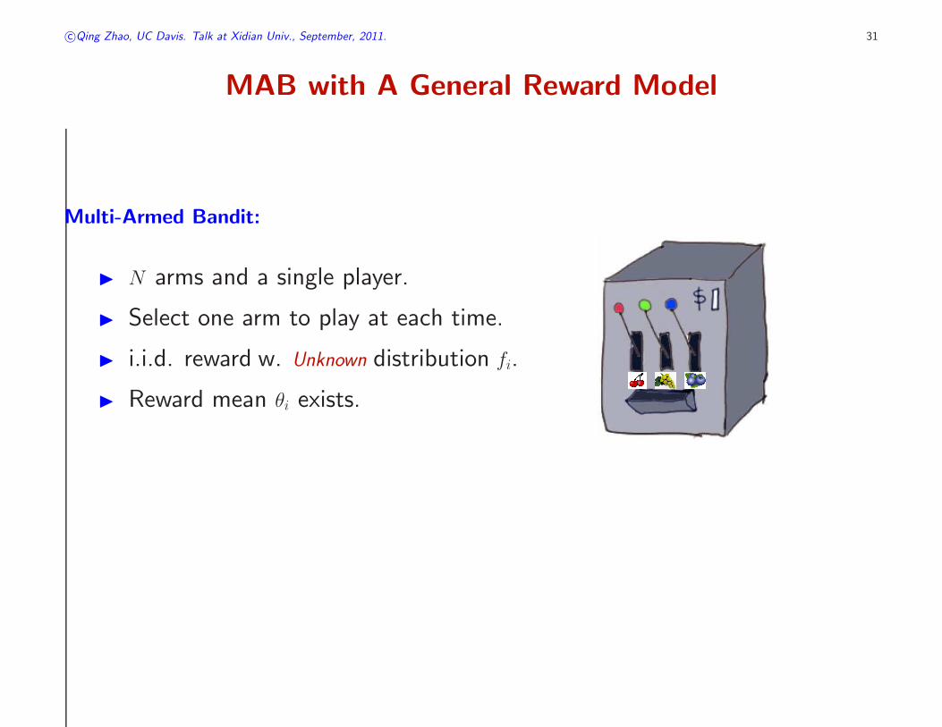
Multi-Armed Bandit:
◮ N arms and a single player.
◮ Select one arm to play at each time.
◮ i.i.d. reward w. Unknown distribution fi.
◮ Reward mean θi exists.

c©Qing Zhao, UC Davis. Talk at Xidian Univ., September, 2011. 32
Sufficient Statistics
Sufficient Statistics:
◮ Sample mean θ̄i(t) (exploitation);
◮ Number of plays τi(t) (exploration);
In the classic policies:
◮ θ̄i(t) and τi(t) are combined together for arm selection at each t:
index = θ̄i +
√
2 log t
τi(t)
◮ A fixed form difficult to adapt to different reward models.

c©Qing Zhao, UC Davis. Talk at Xidian Univ., September, 2011. 33
DSEE
Deterministic Sequencing of Exploration and Exploitation (DSEE):
◮ Time is partitioned into interleaving exploration and exploitation sequences.
��������
��������
������������
������������
������������
������������
��������
��������
��������
��������
��������
��������
������������
������������
t = 1 T
2 Exploration: play all arms in round-robin.
2 Exploitation: play the arm with the largest sample mean.
◮ A tunable parameter: the cardinality of the exploration sequence
2 can be adjusted according to the “hardness” of the reward distributions.
c©Qing Zhao, UC Davis. Talk at Xidian Univ., September, 2011. 34
The Optimal Cardinality of Exploration
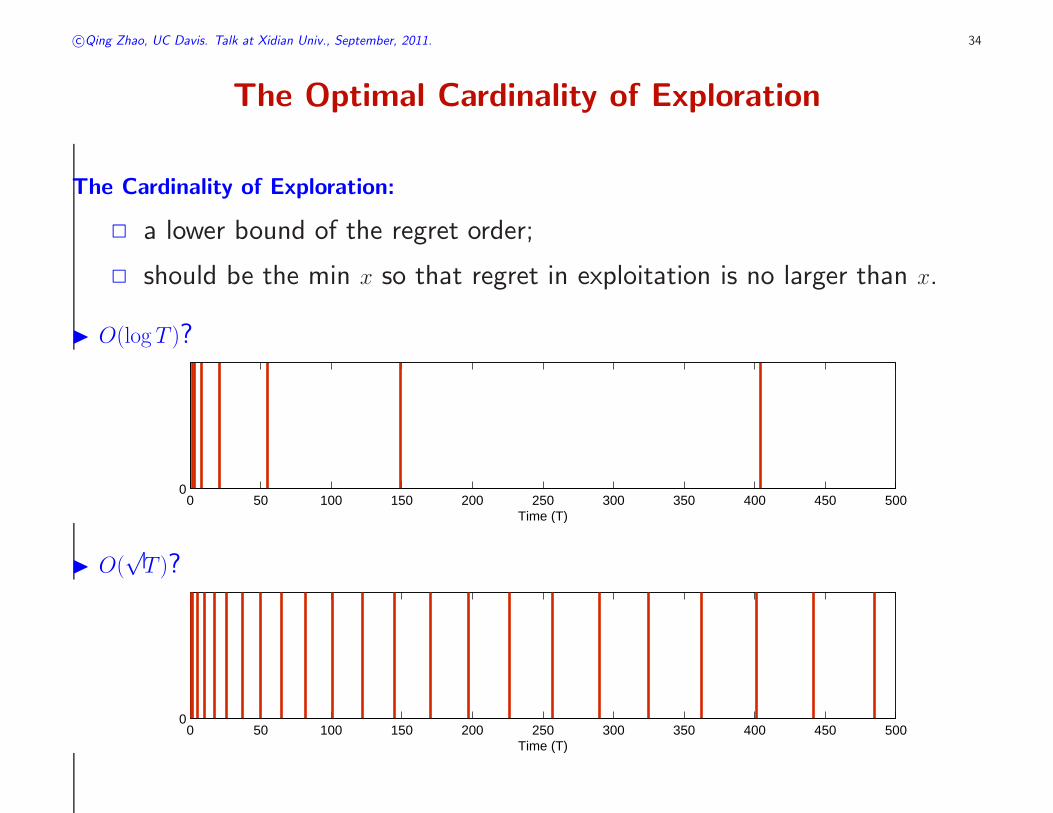
The Cardinality of Exploration:
2 a lower bound of the regret order;
2 should be the min x so that regret in exploitation is no larger than x.
◮ O(log T )?
0 50 100 150 200 250 300 350 400 450 5000
Time (T)
◮ O(√T )?
0 50 100 150 200 250 300 350 400 450 5000
Time (T)

c©Qing Zhao, UC Davis. Talk at Xidian Univ., September, 2011. 35
Performance of DSEE
When moment generating functions of {fi(x)} are properly bounded around 0:
◮ ∃ζ > 0, u0 > 0 s.t. ∀u with |u| ≤ u0,
E[exp((X − θ)u)] ≤ exp(ζu2/2)
◮ DSEE achieves the optimal regret
order O(log T ).
−1 −0.5 0 0.5 11
1.2
1.4
1.6
1.8
2
2.2
2.4
2.6
2.8
u
Mom
ent G
ener
atin
g F
unct
ion
G(u
)
Gaussian (large var.)Gaussian (small var.)Uniform Distribution
When {fi(x)} are heavy-tailed distributions:
◮ The moments of {fi(x)} exist only up to the pth order;
◮ DSEE achieves regret order O(T 1/p).
c©Qing Zhao, UC Davis. Talk at Xidian Univ., September, 2011. 36
Restless Markov Reward Model

c©Qing Zhao, UC Davis. Talk at Xidian Univ., September, 2011. 37
Markov Model
��������������������������������
��������������������������������
������������������������������������
������������������������������������
������������������������������������
������������������������������������
������������������������������������
������������������������������������
��������������������������������
��������������������������������
������������������������������������
������������������������������������
������������������������������������
������������������������������������
Opportunities
Channel 1
Channel N0 1 2 3 T t
t
◮ Channel occupancy: Markovian with unknown transition probabilities:
0 1(busy) (idle)
p01
p11p00
p10
◮ Objective: a channel selection policy to achieve max average reward.

c©Qing Zhao, UC Davis. Talk at Xidian Univ., September, 2011. 38
Markovian Model
Dynamic Spectrum Access under Unknown Model:
��������������������������������
��������������������������������
������������������������������������
������������������������������������
������������������������������������
������������������������������������
������������������������������������
������������������������������������
��������������������������������
��������������������������������
������������������������������������
������������������������������������
������������������������������������
������������������������������������
Opportunities
Channel 1
Channel N0 1 2 3 T t
t
◮ Challenges:
2 The optimal policy under known model is not staying on one channel.
2 Need to learn the best way to switch among channels based on
observations (infinite possibilities).

c©Qing Zhao, UC Davis. Talk at Xidian Univ., September, 2011. 39
Optimal Policy under Known Model
Restless Multi-Armed Bandit:
◮ Whittle index (Whittle:88).
◮ PSPACE-hard in general (Papadimitriou-Tsitsiklis:99).
Optimality of Whittle Index:
(Zhao-Krishnamachari:07,Ahmad-Liu-Javidi-Zhao-Krishnamachari:09,Liu-Zhao:10)
◮ When p11 ≥ p01, holds for all N and K;
◮ When p11 < p01, holds for N = 2, 3 or K = N − 1 (conjectured for all N).
0 1(busy) (idle)
p01
p11p00
p10

c©Qing Zhao, UC Davis. Talk at Xidian Univ., September, 2011. 40
Optimal Policy under Known Model
Semi-Universal Structure of Whittle Index Policy: (Zhao-Krishnamachari:07,Liu-Zhao:10)
◮ When p11 ≥ p01, stay at “idle” and switch at “busy” to the channel visited
longest time ago.
◮ When p11 < p01, stay at “busy” and switch at “idle” to the channel most
recently visited among all channels visited an even number of slots ago
or the channel visited longest time ago.
c©Qing Zhao, UC Davis. Talk at Xidian Univ., September, 2011. 41
Achieving Optimal Throughput under Unknown Model
Achieving Optimal Throughput under Unknown Model:
◮ Treat each way of channel switching as an arm.
◮ Learn which arm is the good arm.
Challenges in Achieving Sublinear Regret:
◮ How long to play each arm: the optimal length L∗ depends on the
transition probabilities.
◮ Rewards are not i.i.d. in time or across arms.
c©Qing Zhao, UC Davis. Talk at Xidian Univ., September, 2011. 42
Achieving Optimal Throughput under Unknown Model
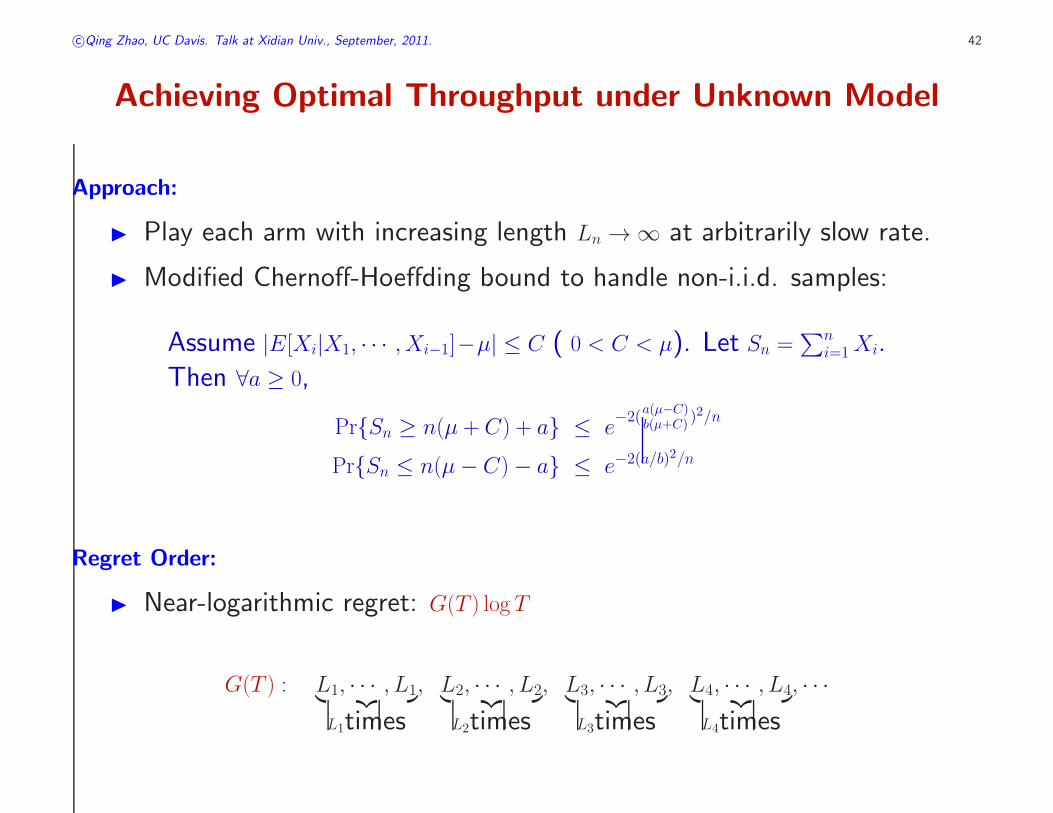
Approach:
◮ Play each arm with increasing length Ln → ∞ at arbitrarily slow rate.
◮ Modified Chernoff-Hoeffding bound to handle non-i.i.d. samples:
Assume |E[Xi|X1, · · · , Xi−1]−µ| ≤ C ( 0 < C < µ). Let Sn =∑n
i=1Xi.
Then ∀a ≥ 0,
Pr{Sn ≥ n(µ + C) + a} ≤ e−2(
a(µ−C)b(µ+C)
)2/n
Pr{Sn ≤ n(µ− C)− a} ≤ e−2(a/b)2/n
Regret Order:
◮ Near-logarithmic regret: G(T ) log T
G(T ) : L1, · · · , L1︸ ︷︷ ︸
L1times
, L2, · · · , L2︸ ︷︷ ︸
L2times
, L3, · · · , L3︸ ︷︷ ︸
L3times
, L4, · · · , L4︸ ︷︷ ︸
L4times
, · · ·
c©Qing Zhao, UC Davis. Talk at Xidian Univ., September, 2011. 43
General Restless MAB with Unknown Dynamics
General Restless MAB with Unknown Dynamics:
◮ Rewards from successive plays form a MC with unknown transition Pi.
◮ When passive, arm evolves a.t. an arbitrary unknown random process.
Difficulty:
◮ Restless MAB under known model itself is intractable in general.
◮ The optimal policy under known model is no longer staying on one arm.
Weak Regret:
◮ Defined with respect to the optimal single-arm policy under known model:
RπT = Tθ(1) − V π
T +O(1).
◮ Best arm: the largest reward mean θ(1) in steady state.
c⃝Qing Zhao, UC Davis. ICASSP, May, 2011. 11
Restless MAB under Unknown Dynamics
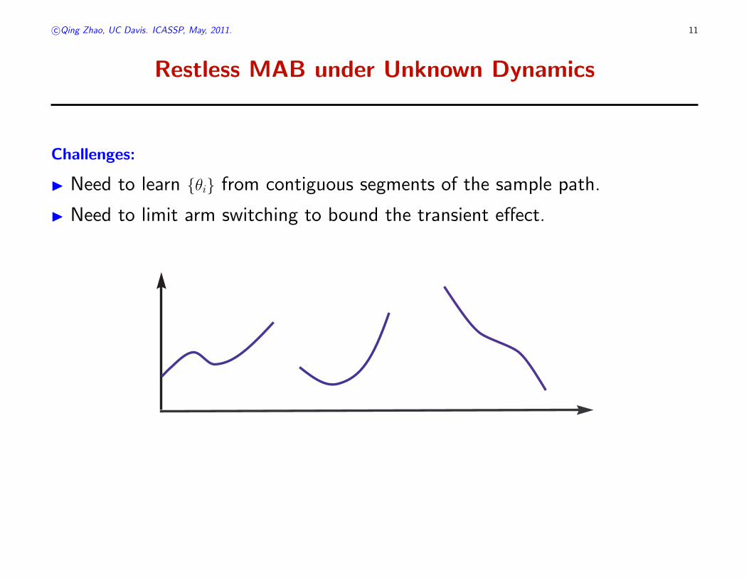
Challenges:
I Need to learn {θi} from contiguous segments of the sample path.
I Need to limit arm switching to bound the transient effect.

c⃝Qing Zhao, UC Davis. ICASSP, May, 2011. 12
Restless UCB Policy
Restless UCB (RUCB):
I Epoch structure with geometrically growing epoch length
I =⇒ arm switching limited to log order.
I Exploration and exploitation epochs interleaving for fast error decay:
2 In exploration epochs, play all arms in turn.
2 In exploitation epochs, play the arm with the largest index s̄i +√
L log tti
.
2 Start an exploration epoch iff total exploration time < D log t.
Exploit "best" arm
Arm 1 Arm 2 Arm 3

c©Qing Zhao, UC Davis. Talk at Xidian Univ., September, 2011. 46
The Logarithmic Regret of RUCB
Logarithmic regret of RUCB:
◮ Uniformly bounded leading constant determined by D and L.
◮ Choosing D and L requires
2 an arbitrary (nontrivial) lower bound on the eigenvalue gaps of Pi.
2 an arbitrary (nontrivial) lower bound on θ(1) − θ(2).
Near logarithmic regret in the absence of system knowledge:
◮ For any increasing sequence f(t),
RRUCB(t) ∼ O(f(t) log t)
◮ by choosing D(t) and L(t) as increasing sequences satisfying
D(t) = f(t),L(t)
D(t)→ 0.

c©Qing Zhao, UC Davis. Talk at Xidian Univ., September, 2011. 47
Decentralized Bandit with Multiple Players
c©Qing Zhao, UC Davis. Talk at Xidian Univ., September, 2011. 48
Decentralized Multi-Armed Bandit
Decentralized Bandit with Multiple Players:
◮ N arms with unknown reward statistics (θ1, · · · , θN).
◮ M (M < N) distributed players.
◮ Each player selects one arm to play and observes the reward.
◮ Distributed decision making using only local observations.
◮ Colliding players either share the reward or receive no reward.
c©Qing Zhao, UC Davis. Talk at Xidian Univ., September, 2011. 49
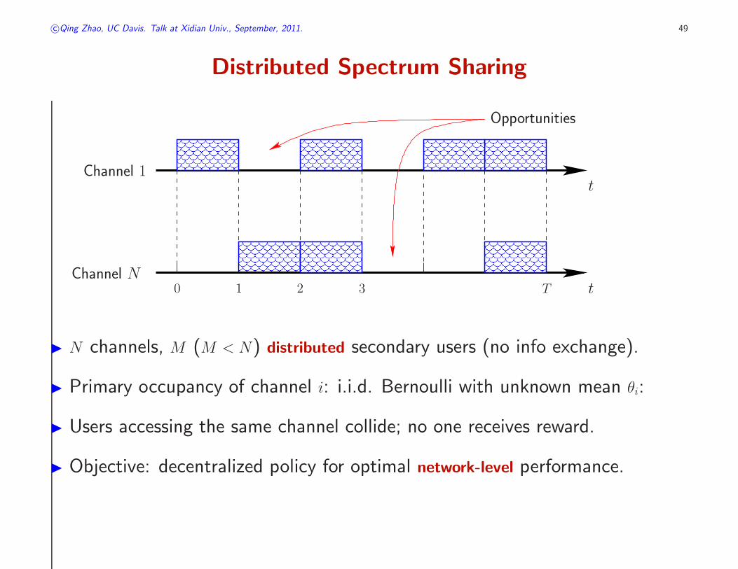
Distributed Spectrum Sharing
��������������������������������
��������������������������������
������������������������������������
������������������������������������
������������������������������������
������������������������������������
������������������������������������
������������������������������������
��������������������������������
��������������������������������
������������������������������������
������������������������������������
������������������������������������
������������������������������������
Opportunities
Channel 1
Channel N0 1 2 3 T t
t
◮ N channels, M (M < N) distributed secondary users (no info exchange).
◮ Primary occupancy of channel i: i.i.d. Bernoulli with unknown mean θi:
◮ Users accessing the same channel collide; no one receives reward.
◮ Objective: decentralized policy for optimal network-level performance.

c©Qing Zhao, UC Davis. Talk at Xidian Univ., September, 2011. 50
Decentralized Multi-Armed Bandit
System Regret:
◮ Total system reward with known (θ1, · · · , θN) and centralized scheduling:
T ΣMi=1 θ(i)︸︷︷︸
ith best
◮ V πT (Θ) : total system reward under a decentralized policy π.
◮ System regret:
RπT (Θ) = TΣM
i=1θ(i) − V π
T (Θ)

c©Qing Zhao, UC Davis. Talk at Xidian Univ., September, 2011. 51
The Minimum Regret Growth Rate
The Minimum regret rate in Decentralized MAB is logarithmic.
R∗T (Θ) ∼ C(Θ) log T
The Key to Achieving log T Order:
◮ Learn from local observations which channels are the most rewarding.
◮ Learn from collisions to achieve efficient sharing with other users.

c©Qing Zhao, UC Davis. Talk at Xidian Univ., September, 2011. 52
Conclusion and Acknowledgement
◮ Bayesian Formulation: A Class of Restless Multi-Armed Bandit:
2 Indexability and optimality of Whittle index: K.Liu&Q.Zhao:08-10.
2 Extension to non-Markovian systems: K.Liu&R.Weber&Q.Zhao:11.
2 Structure and optimality of myopic policy:
Q.Zhao&B.Krishnamachari:07-08,
S.Ahmad&M.Liu&T.Javidi&Q.Zhao&B.Krishnamachari:09.
◮ Non-Bayesian Formulation:
2 From exponential family to general (heavy-tailed) unknown distributions:
K.Liu-Q.Zhao:11.
2 From i.i.d. to restless Markov reward models:
Dai-Gai-Krishnamachari-Zhao:11, H.Liu-K.Liu-Q.Zhao:11.
2 From single player to multiple distributed players:
K.Liu-Q.Zhao:10, H.Liu-K.Liu-Q.Zhao:11