The Multi-Armed Bandit, with ConstraintsEric V. Denardo,1 Eugene A. Feinberg2 and Uriel G. Rothblum3

December 12, 2011

AbstractThe early sections of this paper present an analysis of a Markov decision model that is known as themulti-armed bandit under the assumption that the utility function of the decision maker is either linearor exponential. The analysis includes efficient procedures for computing the expected utility associatedwith the use of a priority policy and for identifying a priority policy that is optimal. The methodologyin these sections is novel, building on the use of elementary row operations. In the later sections of thispaper, the analysis is adapted to accommodate constraints that link the bandits.

1 Introduction

The colorfully-named multi-armed bandit [10] is the following Markov decision problem: At epochs 1, 2, . . . ,a decision maker observes the current state of each of several Markov chains with rewards (bandits) and playsone of them. The Markov chains that are not played remain in their current states. The Markov chain thatis played evolves for one transition according to its transition probabilities, earning an immediate reward(possibly negative) that can depend upon its current state and on the state to which transition occurs. Hence-forth, to distinguish the states of the individual Markov chains from those of the Markov decision problem,the latter are called multi-states; each multi-state prescribes a state for each of the Markov chains.

A key result for the multi-armed bandit is that attention can be restricted to a simple class of decisionprocedures that are based on “labelings.” A labeling is an assignment of a number to each state of eachbandit such that no two states have the same number (label), even if they are in different bandits. A priorityrule is a policy that is determined by a labeling in this way; given each multi-state, the priority rule playsthe Markov chain whose current state has the lowest label. In a seminal 1974 paper, Gittins and Jones [12](followed by [10]) demonstrated the optimality of a priority rule for a model whose objective is to maximizeexpected discounted income with a per-period discount factor c having 0 < c < 1. The (optimal) prioritiesthat they identified are based on a family of stopping times, one for each state of each chain. Given statei of bandit k, the decision maker is imagined to play bandit k for any number τ (τ ≥ 1) of consecutiveepochs, observing the state to which each transition occurs, and stopping whenever he or she wishes to doso. The discounted present value of the (random) income stream that is received during epochs 1 through τ

is denoted X(τ). The stopping times τ for state i are used to assign that state an index I(i) by

I(i) = maxτ

{E[X(τ ]

1− E[cτ ]

}. (1.1)

1Center for Systems Sciences, Yale University, PO Box 208267, New Haven, CT 06520, USA.2Department of Applied Mathematics and Statistics, Stony Brook University, Stony Brook, NY 11794-3600, USA.3Faculty of Industrial Engineering and Management, Technion – Israel Institute of Technology, Haifa 32000, Israel.

1

It was demonstrated in [12, 10] that, given each multi-state, it is optimal to play any Markov chain (bandit)whose current state has the largest index (lowest label).

Following [12, 10], the multi-armed bandit problem has stimulated research in control theory, eco-nomics, probability, and operations research. A sampling of noteworthy papers includes Bergemann andValimakim [2], Bertsimas and Nino-Mora [4], El Karoui and Karatzas [8], Katehakis and Veinott [15],Schlag [17], Sonin [18], Tsisiklis [19], Variaya, Walrand and Buyukkoc [20], Weber [22], and Whittle [24],.Books on the subject (that list many references) include Berry and Fristedt [3], Gittins [11], Gittins, Glaze-brook and Weber [13]. The last and most recent of these books provides a status report on the multi-armedbandit that is almost up-to-date.

An implication of the analysis in [12, 10] is that the largest of all of the indices equals the maximum overall states of the ratio r(i)/(1 − c), where r(i) denotes the expectation of the reward that is earned if statei’s bandit is played once while state i is observed and where c is the discount factor. In 1994, Tsitsiklis [19]observed that repeated play of a bandit while it is in the state i whose ratio is largest leads to a multi-armedbandit with one fewer state and random transition times.

In 2007 Denardo, Park and Rothblum [6] considered a generalization of classic multi-armed banditmodel with the following new features:

• The utility function of the decision maker can be exponential, expressing sensitivity to risk.

• In the case of linear utility functions, the assumption that rewards are discounted is replaced by theintroduction of stopping (which captures discounting).

The analysis of [6] focused on pair-wise comparisons It avoided the use of stopping times, which had beena common feature of the prior analyses of multi-armed bandits. It relied on linear algebra, rather than onprobability theory. It avoided the need to deal, in the more general cases, with ratios that had zeros in theirdenominators. It included efficient algorithms for computing indices and for identifying an optimal priorityrule.

Constraints that link the bandits (for the extension considered in [6]) are dealt with in Sections 7-8 ofthe current paper. An optimal solution to the multi-armed bandit problem with W constraints is shown to bean initial randomization over W +1 priority rules, each of which is the optimal solution to an unconstrainedbandit problem whose rewards are determined by a particular set of prices (multipliers) on the constraints.A column generation algorithm is described for computing such an optimal solution. In each stage, thecoefficients of the column that enters the basis are found by the application of the policy evaluation procedureof Section 4.

As concerns contributions to methodology, the analysis in the earlier sections of this paper rests onelementary row operations. Row operations are used in sections 3-4 to present the first efficient algorithmfor computing the utility function gained when beginning at a given multi-state and using any given priorityrule (solving the optimality equation is inefficient as the number of multi-states can be enormous). Rowoperations are also used in Section 5-6 to determine efficiently an optimal priority policy and to provide aproof for its optimality. The approach in the current paper builds on that of [6], but simplifies the theoreticaldevelopment and the computation. In particular, the computation effort that the method requires matches the

2

best existing bound for computing Gittins indices (obtained in [16], see [13, p.43] (in fact, the same boundapplies to the method developed in [6]).

2 The model

Let K be the number of Markov chains (bandits), and let them be numbered 1 through K. Markov chain k

has a finite set Nk of states. No loss of generality occurs by assuming, as we do, that the states of distinctMarkov chains are disjoint. Thus, each state j identifies the Markov chain b(j) of which it is a member, i.e.,j ∈ Nb(j). The set of all states of all bandits is given by N = N1 ∪ · · · ∪NK .

If bandit k is played while its state is i, this bandit experiences transition to state j with probabilityp(i, j), and it experiences termination of play with probability p(i, 0) given by

p(i, 0) = 1−∑j∈Nk

p(i, j) ∀ i ∈ Nk, ∀ k ∈ {1, 2, . . . ,K} .

If bandit k is played when its state is i and if transition is to occur to state j, payoff x(i, j) is earned at thestart of the period; if termination is to occur instead, payoff x(i, 0) is earned at the start of the period. Eachof these “payoffs” can be positive, negative or zero.

Termination stops the play of all K bandits, not merely of the bandit that is being played. Terminationis modeled as transition to state 0. No action is possible after transition to state 0. For this reason, state 0 isexcluded from Nk for each k, and hence from N .

Each multi-state s is a set that contains, for each k, exactly one state in Nk. When s is a multi-state, thesymbol sk denotes the state of bandit k that is included in s, and the symbol s\k is defined by s\k = s\{sk}.Thus, s\k contains all the states in s other than sk. Let S denote the set of all multi-states. Given any multi-state s, one of the bandits must be played. Hence, for this model, a stationary nonrandomized policy δ isany map that for each multi-state s ∈ S picks a bandit δ(s) ∈ {1, 2, . . . ,K}. Let ∆ denote the set of allstationary nonrandomized policies.

2.1 Utility

The goal is to maximize expected utility. This will be accomplished with a linear utility function u(x) = x,with a risk-averse exponential utility function u(x) = −e−λx where λ is a positive constant that is knownas the coefficient of risk aversion and with a risk-seeking exponential utility function u(x) = eλx where λ isa positive constant.

All three cases are described and analyzed using the local utility function h(s, k, v) whose value equalsthe expectation of the total utility that is earned in the (artificially-truncated) one-transition model if multi-state s is observed now, if bandit k is selected now, and if utility v(t) is earned if transition occurs tomulti-state t.

3

2.2 Linear utility

In the case of linear utility, the local utility function is

h(s, k, v) = r(sk) +∑j∈Nk

q(sk, j)v(s\k ∪ {j}) , (2.1)

with data r(i) and q(i, j) that are specified by

r(i) = p(i, 0)x(i, 0) +∑

j∈Nb(i)

p(i, j)x(i, j) ∀ i ∈ N , (2.2)

q(i, j) = p(i, j) , ∀ i, j ∈ Nk , ∀ k ∈ {1, 2, . . . ,K} . (2.3)

Interpret r(i) as the expectation of the reward that is earned immediately if bandit b(i) is played while itsstate is i, and interpret q(i, j) as the probability that bandit b(i) will experience transition to state j giventhat it is played while its state is i. As noted earlier, playing bandit b(i) while its state is i causes termination(rather than transition to some state j in Nb(i)) with probability p(i, 0), which may be positive. The abovemodel captures the classic discounted model, which has transition probability p(i, j) and discount factor csatisfying 0 < c < 1, by replacing p(i, 0) and p(i, j) in (2.2)-(2.3) by cp(i, 0) and cp(i, j), respectively.Incorporating the discount factor into the transition rates yields a fundamental advantage – it facilitates ananalysis that applies linear algebraic arguments instead of stopping times.

2.3 Exponential utility

With the risk-averse exponential utility function u(x) = −e−λx, one has u(x + y) = −e−λ(x+y) =

e−λxu(y), and the local utility function is given by (2.1) with data r(i) and q(i, j) that are specified, foreach i ∈ N and j ∈ Nb(i), by

r(i) = −p(i, 0) e−λx(i,0) and q(i, j) = p(i, j) e−λx(i,j). (2.4)

With the risk-seeking exponential utility function u(x) = eλx, the local utility function is given by (2.1)with data

r(i) = p(i, 0) eλx(i,0) and q(i, j) = p(i, j) eλx(i,j). (2.5)

With all three utility functions, r(i) is called a reward, and q(i, j) is called a transition rate. In the linear-utility model, q(i, j) is a probability. In the risk-averse exponential-utility model, q(i, j) is the product of aprobability and a disutility.

Bandit k has an |Nk| × |Nk| matrix qk whose ijth entry equals q(i, j) for each ordered pair (i, j) ofstates in Nk. In each case, the entries in qk are nonnegative. In the linear-utility case, qk is substochastic,which is to say that its entries are nonnegative and the entries in each row sum to 1 or less. In the risk-averseexponential case, each state i has reward r(i) ≤ 0. In the risk-seeking exponential case, each state i hasreward r(i) ≥ 0.

4

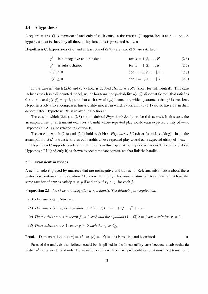
2.4 A hypothesis

A square matrix Q is transient if and only if each entry in the matrix Qt approaches 0 as t → ∞. Ahypothesis that is shared by all three utility functions is presented below as:

Hypothesis C. Expressions (2.6) and at least one of (2.7), (2.8) and (2.9) are satisfied.

qk is nonnegative and transient for k = 1, 2, . . . ,K . (2.6)

qk is substochastic for k = 1, 2, . . . ,K . (2.7)

r(i) ≤ 0 for i = 1, 2, . . . , |N | . (2.8)

r(i) ≥ 0 for i = 1, 2, . . . , |N | . (2.9)

In the case in which (2.6) and (2.7) hold is dubbed Hypothesis RN (short for risk neutral). This caseincludes the classic discounted model, which has transition probability p(i, j), discount factor c that satisfies0 < c < 1 and q(i, j) = cp(i, j), so that each row of (qk)t sums to c, which guarantees that qk is transient.Hypothesis RN also encompasses linear-utility models in which ratios akin to (1.1) would have 0’s in theirdenominator. Hypothesis RN is relaxed in Section 10.

The case in which (2.6) and (2.8) hold is dubbed Hypothesis RA (short for risk-averse). In this case, theassumption that qk is transient excludes a bandit whose repeated play would earn expected utility of −∞.Hypothesis RA is also relaxed in Section 10.

The case in which (2.6) and (2.9) hold is dubbed Hypothesis RS (short for risk-seeking). In it, theassumption that qk is transient rules out bandits whose repeated play would earn expected utility of +∞.

Hypothesis C supports nearly all of the results in this paper. An exception occurs in Sections 7-8, whereHypothesis RN (and only it) is shown to accommodate constraints that link the bandits.

2.5 Transient matrices

A central role is played by matrices that are nonnegative and transient. Relevant information about thesematrices is contained in Proposition 2.1, below. It employs this nomenclature; vectors x and y that have thesame number of entries satisfy x≫ y if and only if xj > yj for each j.

Proposition 2.1. Let Q be a nonnegative n× n matrix. The following are equivalent:

(a) The matrix Q is transient.

(b) The matrix (I −Q) is invertible, and (I −Q)−1 = I +Q+Q2 + · · · .

(c) There exists an n× n vector f ≫ 0 such that the equation (I −Q)x = f has a solution x≫ 0.

(d) There exists an n× 1 vector y ≫ 0 such that y ≫ Qy.

Proof. Demonstration that (a)⇒ (b)⇒ (c)⇒ (d)⇒ (a) is routine and is omitted.

Parts of the analysis that follows could be simplified in the linear-utility case because a substochasticmatrix qk is transient if and only if termination occurs with positive probability after at most |Nk| transitions.

5

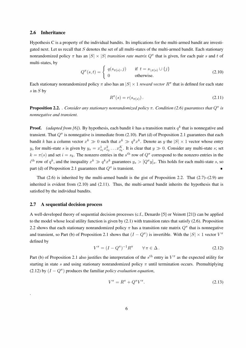
2.6 Inheritance

Hypothesis C is a property of the individual bandits. Its implications for the multi-armed bandit are investi-gated next. Let us recall that S denotes the set of all multi-states of the multi-armed bandit. Each stationarynonrandomized policy π has an |S| × |S| transition rate matrix Qπ that is given, for each pair s and t ofmulti-states, by

Qπ(s, t) =

{q(sπ(s), j) if t = s\π(s) ∪ {j}0 otherwise.

(2.10)

Each stationary nonrandomized policy π also has an |S| × 1 reward vector Rπ that is defined for each states in S by

Rπ(s) = r(sπ(s)) . (2.11)

Proposition 2.2. . Consider any stationary nonrandomized policy π. Condition (2.6) guarantees that Qπ isnonnegative and transient.

Proof. (adapted from [6]). By hypothesis, each bandit k has a transition matrix qk that is nonnegative andtransient. That Qπ is nonnegative is immediate from (2.10). Part (d) of Proposition 2.1 guarantees that eachbandit k has a column vector xk ≫ 0 such that xk ≫ qkxk. Denote as y the |S| × 1 vector whose entryys for multi-state s is given by ys = x1s1x

2s2 . . . x

Ksk

. It is clear that y ≫ 0. Consider any multi-state s; setk = π(s) and set i = sk. The nonzero entries in the sth row of Qπ correspond to the nonzero entries in theith row of qk, and the inequality xk ≫ qkxk guarantees ys > [Qπy]s. This holds for each multi-state s, sopart (d) of Proposition 2.1 guarantees that Qπ is transient.

That (2.6) is inherited by the multi-armed bandit is the gist of Proposition 2.2. That (2.7)–(2.9) areinherited is evident from (2.10) and (2.11). Thus, the multi-armed bandit inherits the hypothesis that issatisfied by the individual bandits.

2.7 A sequential decision process

A well-developed theory of sequential decision processes (c.f., Denardo [5] or Veinott [21]) can be appliedto the model whose local utility function is given by (2.1) with transition rates that satisfy (2.6). Proposition2.2 shows that each stationary nonrandomized policy π has a transition rate matrix Qπ that is nonnegativeand transient, so Part (b) of Proposition 2.1 shows that (I − Qπ) is invertible. With the |S| × 1 vector V π

defined byV π = (I −Qπ)−1Rπ ∀π ∈ ∆ . (2.12)

Part (b) of Proposition 2.1 also justifies the interpretation of the sth entry in V π as the expected utility forstarting in state s and using stationary nonrandomized policy π until termination occurs. Premultiplying(2.12) by (I −Qπ) produces the familiar policy evaluation equation,

V π = Rπ +QπV π. (2.13)

.

6

With the |S| × 1 vector F defined by

F (s) = max{V δ(s) : δ ∈ ∆

}∀ s ∈ S , (2.14)

the number F (s) equals the largest expected utility obtainable from any stationary nonrandomized policy,given starting state s. A policy π is said to be optimal if V π = F . The restriction to stationary nonrandom-ized policies is justified because Hypothesis C has been shown to suffice for such a policy to be optimal overthe class of all history-remembering policies, see [5] or [21]. Further, such a policy can be found by linearprogramming, by policy improvement, or by successive approximation. None of these methods is practicalwhen the number |S| of multi-states is large, however.

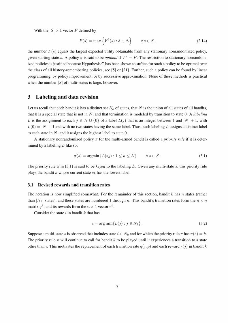
3 Labeling and data revision

Let us recall that each bandit k has a distinct set Nk of states, that N is the union of all states of all bandits,that 0 is a special state that is not in N , and that termination is modeled by transition to state 0. A labelingL is the assignment to each j ∈ N ∪ {0} of a label L(j) that is an integer between 1 and |N | + 1, withL(0) = |N |+1 and with no two states having the same label. Thus, each labeling L assigns a distinct labelto each state in N , and it assigns the highest label to state 0.

A stationary nonrandomized policy π for the multi-armed bandit is called a priority rule if it is deter-mined by a labeling L like so:

π(s) = argmin {L(sk) : 1 ≤ k ≤ K} ∀ s ∈ S . (3.1)

The priority rule π in (3.1) is said to be keyed to the labeling L. Given any multi-state s, this priority ruleplays the bandit k whose current state sk has the lowest label.

3.1 Revised rewards and transition rates

The notation is now simplified somewhat. For the remainder of this section, bandit k has n states (ratherthan |Nk| states), and these states are numbered 1 through n. This bandit’s transition rates form the n × n

matrix qk, and its rewards form the n× 1 vector rk.Consider the state i in bandit k that has

i = argmin{L(j) : j ∈ Nk} . (3.2)

Suppose a multi-state s is observed that includes state i ∈ Nk and for which the priority rule π has π(s) = k.The priority rule π will continue to call for bandit k to be played until it experiences a transition to a stateother than i. This motivates the replacement of each transition rate q(j, p) and each reward r(j) in bandit k

7

by q(j, p) and r(j), where:

q(i, p) = q(i, p)/[1− q(i, i)] if p = i , (3.3)

q(j, p) = q(j, p) + q(j, i)q(i, p) if j = i and p = i , (3.4)

q(j, i) = 0 for each j , (3.5)

r(i) = r(i)/[1− q(i, i)] , (3.6)

r(j) = r(j) + q(j, i)r(i) if j = i . (3.7)

The selection of i borrows from [19], but that reference does not suggest any scheme to update the data asis done in (3.3)-(3.7).

Repeated play replaces the bandit’s transition rate matrix qk by the matrix qk whose entries are givenby (3.3)–(3.5), and it replaces the bandit’s reward vector rk by the vector rk whose entries are given by(3.6)–(3.7). The revised transition matrix and reward vector are for a model in which transitions to state i

do not occur. It will soon be demonstrated that qk and rk inherit the version of Hypothesis C that is satisfiedby qk and rk.

3.2 Elementary row operations

Equations (3.4), (3.5) and (3.7) describe a model in which the data of bandit k has been revised so thatno transitions occur to the state i. This process can be iterated. The second execution of (3.2) occurswith state i removed from Nk, and it selects the state i in Nk whose label is second lowest. And so forth.Algorithmically, the effect of repeated data revision is to begin with the n × (n + 1) matrix (tableau)[(I − qk), rk] and to use elementary row operations to alter the entries in this tableau like so:

Triangularizer (for bandit k in accord with labeling L).

1. Begin with the tableau [(I − qk), rk]. Set M = Nk. While M is nonempty, do Steps 2 and 3.

2. Find the state i ∈M whose label L(i) is smallest. Set α = 1/[1− qk(i, i)].

(a) Replace row i of the tableau [(I − qk), rk] by itself times the constant α.

(b) For each state j ∈M \ {i}, replace row j of this tableau by itself plus the constant q(j, i) times(the updated) row i; this update equates qjt to 0 for t = i and for each t in N \M .

3. Replace M by M \ {i}.

The first execution of Step 2 replaces the tableau [(I − qk), rk] by [(I − qk), rk] where the entries in then × 1 vector rk and in the n × n matrix qk are specified by (3.3)–(3.7) with i as the state whose label islowest. The second execution of Step 2 replaces qk by the transition rate matrix qk for which transitions tostate i are not observed and in which transitions to the state i whose label is second lowest are not observed,except for transition from i to i. And so forth.

Proposition 3.1. Suppose that the data for bandit k satisfy Hypothesis RN, RA, or RS. When the datafor bandit k are triangulated in accord with a labeling L, each iteration of Step 2 produces a tableau[(I − qk), rk] that satisfies the same hypothesis.

8

Proof. By hypothesis, qk is nonnegative and transient. The initial execution of Step 2 of the Triangularizerreplaces [(I − qk), rk] by [(I − qk), rk]. It does so by multiplying row i by the positive number α and thenreplacing each row j other than i by itself plus the nonnegative multiple q(j, i) times the updated row (i).This guarantees qk ≥ 0. It further guarantees that rk ≤ 0 if rk ≤ 0 and that rk ≥ 0 if rk ≥ 0. In particular,(2.8) and (2.9) are preserved.

Since qk is nonnegative and transient, Part (c) of Proposition 2.1 shows that there exists a vector f ≫ 0

such that the equation (I − qk)x = f has a solution x ≫ 0. Let us apply the Triangularizer to the tableau[(I−qk), f ]. The initial execution of Step 2 replaces [(I−qk), f ] by [(I−qk), f ]. Elementary row operationspreserve the solutions to equation systems, so the strictly positive vector x satisfies (I − qk)x = f . Sinceqk ≥ 0, part (c) of Proposition 2.1 also shows that qk is transient, hence that (2.6) is preserved.

Finally, suppose that qk satisfies (2.7). With e as the n × 1 vector of 1’s, note that (I − qk)e = g withg ≥ 0. As noted above, (I − qk)e = g with g ≥ 0, which shows that (2.7) is preserved.

It has been demonstrated that Hypotheses RN, RA and RS are preserved by the first execution of Step 2of the Triangularizer. Iterating this argument completes the proof.

The computational effort for executing the Triangularizer is determined in the next result.

Proposition 3.2. With n ≡ |Nk|, executing the Triangularizer on bandit k entails 23 |n|

3 − 12 |n|

2 + 23 |n|

arithmetic operations.

Proof. The computation of the [1−qk(i, i)]’s is Step 1 requires n subtractions. Next consider the executionof Step 2 when |M | = m. As the entries in row i indexed by the columns of Nk \M are zero and are notchanged in Substep 2(a) and as 1−qk(i,i)

1−qk(i,i)= 1, Substep 2(a) requires m divisions (including the update or

rk(i)). Also, Substep 2(b) requires (m − 1)m additions and (m − 1)m multiplications. Thus, the totalnumber of arithmetic operation needed to execute both substeps is m + 2m(m − 1) = 2m2 − m. As∑n

m=1m2 =

∑nm=1 2

(m2

)+

(m1

)= 2

(n+13

)+

(n+12

)= 1

3n3 + 1

2n2 + 1

6n and∑n

m=1m = n2+n2 , the total

number of arithmetic operations needed to execute the triangularizer is n+ 2[13n3 + 1

2n2 + 1

6n]−n2+n

2 =23n

3 − 12n

2 + 23n.

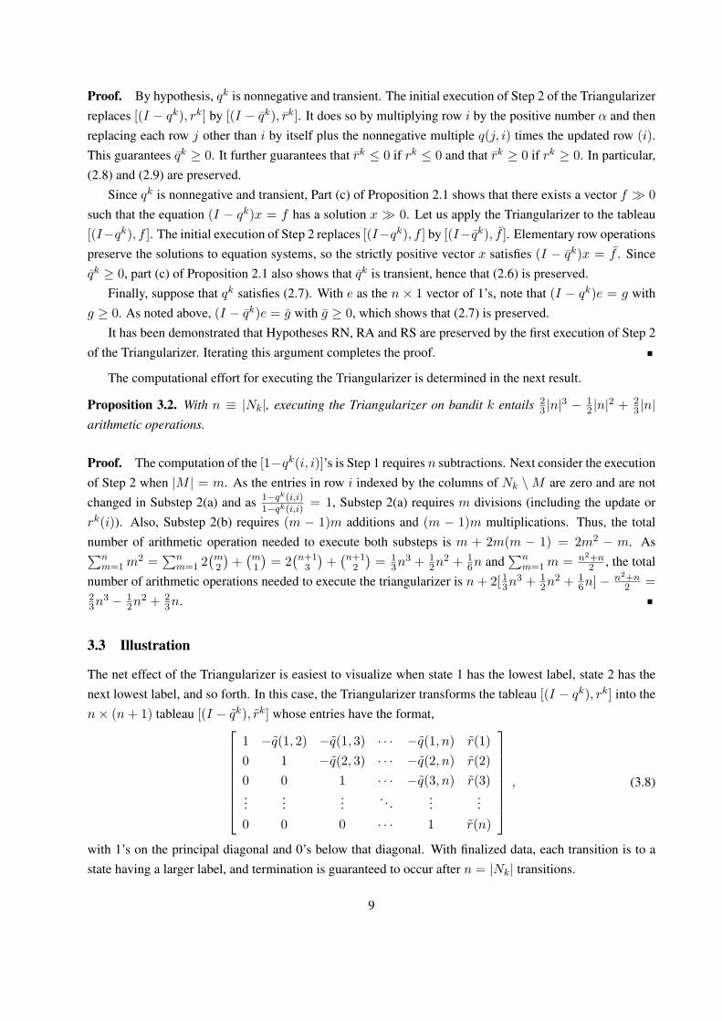
3.3 Illustration

The net effect of the Triangularizer is easiest to visualize when state 1 has the lowest label, state 2 has thenext lowest label, and so forth. In this case, the Triangularizer transforms the tableau [(I − qk), rk] into then× (n+ 1) tableau [(I − qk), rk] whose entries have the format,

1 −q(1, 2) −q(1, 3) · · · −q(1, n) r(1)

0 1 −q(2, 3) · · · −q(2, n) r(2)

0 0 1 · · · −q(3, n) r(3)...

......

. . ....

...0 0 0 · · · 1 r(n)

, (3.8)

with 1’s on the principal diagonal and 0’s below that diagonal. With finalized data, each transition is to astate having a larger label, and termination is guaranteed to occur after n = |Nk| transitions.

9

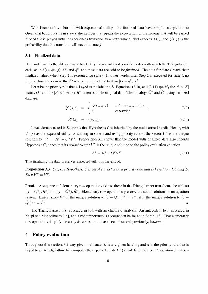
With linear utility—but not with exponential utility—the finalized data have simple interpretations:Given that bandit b(i) is in state i, the number r(i) equals the expectation of the income that will be earnedif bandit k is played until it experiences transition to a state whose label exceeds L(i), and q(i, j) is theprobability that this transition will occur to state j.

3.4 Finalized data

Here and henceforth, tildes are used to identify the rewards and transition rates with which the Triangularizerends, as in r(i), q(i, j), rk, and qk, and these data are said to be finalized. The data for state i reach theirfinalized values when Step 2 is executed for state i. In other words, after Step 2 is executed for state i, nofurther changes occur in the ith row or column of the tableau [(I − qk), rk].

Let π be the priority rule that is keyed to the labeling L. Equations (2.10) and (2.11) specify the |S|×|S|matrix Qπ and the |S| × 1 vector Rπ in terms of the original data. Their analogs Qπ and Rπ using finalizeddata are:

Qπ(s, t) =

{q(sπ(s), j) if t = s\π(s) ∪ {j}0 otherwise

, (3.9)

Rπ(s) = r(sπ(s)) . (3.10)

It was demonstrated in Section 3 that Hypothesis C is inherited by the multi-armed bandit. Hence, withV π(s) as the expected utility for starting in state s and using priority rule π, the vector V π is the uniquesolution to V π = Rπ + QπV π. Proposition 3.1 shows that the model with finalized data also inheritsHypothesis C, hence that its reward vector V π is the unique solution to the policy evaluation equation

V π = Rπ + QπV π . (3.11)

That finalizing the data preserves expected utility is the gist of:

Proposition 3.3. Suppose Hypothesis C is satisfied. Let π be a priority rule that is keyed to a labeling L.Then V π = V π.

Proof. A sequence of elementary row operations akin to those in the Triangularizer transforms the tableau[(I −Qπ), Rπ] into [(I − Qπ), Rπ]. Elementary row operations preserve the set of solutions to an equationsystem. Hence, since V π is the unique solution to (I − Qπ)V π = Rπ, it is the unique solution to (I −Qπ)vπ = Rπ.

The Triangularizer first appeared in [6], with an elaborate analysis. An antecedent to it appeared inKaspi and Mandelbaum [14], and a contemporaneous account can be found in Sonin [18]. That elementaryrow operations simplify the analysis seems not to have been observed previously, however.

4 Policy evaluation

Throughout this section, s is any given multistate, L is any given labeling and π is the priority rule that iskeyed to L. An algorithm that computes the expected utility V π(s) will be presented. Proposition 3.3 shows

10

that V π = V π for which reason V π(s) can - and will be - computed using finalized data. With finalizeddata, for (any given) state i bandit b(i) is played at most once while in state i and the finalized return r(i) isearned if that event occurs. The expected utility V π(s) is then a linear combination of the finalized rewardssay

V π(s) =∑i

z(i)r(i) ; (4.1)

in the case of linear utility, z(i) is the probability that bandit k is played when its state is i, with finalizeddata.

A recursion will be used to compute the z(i)’s. Each step of this recursion updates entries in a set ofvectors, on per bandit. For p = 1, . . . ,K, the vector yp has |Np| entries, one per state, and is initialized by

yp(j) =

{1 if j = sp

0 if j ∈ Np \ {sp}. (4.2)

Successively, for n = 1, 2, . . . , |N |, this procedure selects the state i having L(i) = n, sets k = b(i),updates yk by

yk(j) ← [yk(j) + yk(i)q(i, j)] if j ∈ Nk \ {i} , (4.3)

yk(i) ← 0 , (4.4)

and makes no change in yp for any p = k. Equation (4.3) augments the transition rate yk(j) to state j bythe transition rate yk(i)q(i, j) to state i and then directly to j. Equation (4.4) reflects the fact that no state i

is revisited when finalized data are employed.The analysis of this procedure is eased by defining, for n = 1, 2, . . . , |N |,

Pn = {s ∈ S : n > min{L(sk) : 1 ≤ k ≤ K} . (4.5)

Evidently, Pn contains those multi-states that include a state whose label is less than n.

Proposition 4.1. Suppose Hypothesis C is satisfied. Interrupt the execution of (4.3)–(4.4) just prior tothe iteration in which it selects the state i having L(i) = n. At this moment, the quantity yp(j) equals theaggregate transition rate with finalized data of bandit p from state sp to state j due to play at each multi-statein Pn.

Proof. When n = 1, this result corresponds to the initial conditions. Suppose it holds for n ≥ 1. Expres-sions (4.3) and (4.4) show that it holds for n+ 1.

Proposition 4.1 prepares for the analysis of the:

Evaluator (for starting multi-state s, labeling L and priority rule π that is keyed to L).

1. For each bandit k, define yk by (4.2). Set V = 0 and n = 1. While n ≤ |N |, do Steps 2 and 3.

11

2. Let i be the state whose label L(i) equals n, and set k = b(i). Replace V by

V + r(i)yk(i)∏p=k

∑j∈Np

yp(j)

. (4.6)

3. Execute (4.3) and then (4.4) for bandit k. Then replace n by n+ 1.

The next result shows that the Evaluator determines V π(s).

Proposition 4.2. Suppose Hypothesis C is satisfied. The Evaluator terminates with V = V π(s).

Proof. For i ∈ N , set n = L(i) and k = b(i). The coefficient z(i) in (4.1) equals the aggregate transitionrate from multi-state s to the set of multi-states s that have n = min{L(sp) : 1 ≤ p ≤ K}. From Proposition4.1, we obtain z(i) = yk(i)

∏p =k

[∑j∈Np

yp(j)], which completes the proof.

The computational effort for executing the Evaluator is determined in the next result.

Proposition 4.3. With n ≡∑K

k=1 |Nk|, executing the Evaluator entails∑K

k=132 |Nk|2 + 7

2n− 5 arithmeticoperations (beyond the effort required to apply the Triangularizer on each bandit).

Proof. Augment the evaluator by keeping a record of wp =∑

j∈Npyp(j) for each p and of w =∏|K|

p=1

[∑j∈Np

yp(j)]. The initial value of each of these expressions is 1. Keeping record of these ex-

pression will facilitate the computation of the bracketed terms in (5.5) by a single division.Consider the implementation of Step 2 when i ∈ Nk is selected and m is the number of states in Nk

whose label is lager than L(i). In this case the execution of (5.5) is Step 2 requires one addition, 2 multipli-cations and one division, totalling 4 arithmetic operations. Also, in step 3, (5.2) has to be implemented onlyto the m states in Nk whose label is higher than L(i), requiring m additions and m multiplications, totalling2m arithmetic operations. Next,

∑j∈Np

yp(j) has to be updated only for p = k and this update requires

m − 1 additions. Also, the update of∏|K|

p=1

[∑j∈Np

yp(j)]

requires the multiplication of the old value by

the ratio of the new and old values of∑

j∈Nkyk(j), requiring 2 arithmetic operations. The total number of

arithmetic operation applied to execute steps 2 and 3 over all states i is then

K∑k=1

|Nk|−1∑m=1

(3m+ 5) =K∑k=1

(3|Nk|+ 10)(|Nk| − 1)

2=

K∑k=1

3

2|Nk|2 +

7

2n− 5.

To our knowledge, the computation of V π(s) for a particular priority policy π and particular starting states is new. With a different function (4.2), the Evaluator and its work bound apply to any initial distributionover the multi-states that is in product form (except that the initial values of the wp’s and w of the proof ofTheorem 5.2 will require n-1 additional arithmetic operations).

12

5 Pairwise comparison and preference

In this section, pairwise comparison will be used to identify a state that is “best” amongst a group of states,and the data for that state’s bandit will be revised accordingly. The amplification a(i) of state i is nowdefined by

a(i) =∑

j∈Nb(i)

q(i, j) . (5.1)

Under Hypothesis RN, each amplification is 1 or less. In the risk-averse and risk-seeking cases, some statescan have amplifications that exceed 1, however.

Playing chain b(i) when its state is i earns reward r(i) and multiplies future rewards by the factor a(i).State i is now said to be preferable to state j if

r(i) + a(i)r(j) > r(j) + a(j)r(i) . (5.2)

Suppose that state i is preferable to state j: if a multi-state s is observed that includes states i and j, playingbandit b(i) first and b(j) second is better than the other way around. The definition of preference is appliedeven when states i and j are in the same bandit, however.

It will soon be seen that preference is not transitive, but that it can be refined in a way that is transitive.To this end, states will be grouped into “categories.” The rule by which a category is assigned to each statevaries with the hypothesis.

5.1 Categories under Hypothesis RN

Under Hypothesis RN, each state j has a(j) ≤ 1, and each state is assigned a category by this rule:

• Category 1 consists of each state j that has a(j) = 1 and r(j) ≥ 0.

• Category 2 consists of each state j that has a(j) < 1.

• Category 3 consists of each state j that has a(j) = 1 and r(j) < 0.

It is easy to see that each state j in category 1 that has r(j) > 0 is preferable to every state in category2 and that each state in category 2 is preferable to every state in category 3. But no state in category 1 ispreferable to any state in category 3. For this reason, preference is not transitive. State i is now said to beweakly preferable to state j if the inequality,

r(i) + a(i)r(j) ≥ r(j) + a(j)r(i) , (5.3)

holds strictly or if this inequality holds as an equation and the category of i is at least as small as the categoryof j. Under Hypothesis RN, each state i is assigned a ratio ρ(i) by the following rule:

ρ(i) =

+∞ if state i is in category 1,r(i)/[1− a(i)] if state i is in category 2,−∞ if state i is in category 3.

(5.4)

It is easy to check that state i is weakly preferable to state j if and only if ρ(i) ≥ ρ(j). Evidently,weak preference is transitive. A state i that is weakly preferable to all others can be found with |N | − 1

comparisons.

13

5.2 Categories under Hypothesis RA

Under Hypothesis RA, a state j can have a(j) > 1, but each state j has r(j) ≤ 0, and the states groupthemselves into categories like so:

• Category 1 consists of each state j that has r(j) = 0 and a(j) ≤ 1.

• Category 2 consists of each state j that has r(j) < 0.

• Category 3 consists of each state j that has r(j) = 0 and a(i) > 1.

As before, state i is said to be weakly preferable to state j if (5.3) holds strictly or if (5.3) holds as anequation and the category of state i is at least as small as the category of state j. Under Hypothesis RA, eachstate i is assigned a ratio ρ(i) by this rule:

ρ(i) =

+∞ if state i is in category 1,[1− a(i)] /r(i) if state i is in category 2,−∞ if state i is in category 3.

(5.5)

It is easy to check that i is weakly preferable to state j if and only if ρ(i) ≥ ρ(j).

5.3 Categories under Hypothesis RS

In the risk-seeking case, each state j has r(j) ≥ 0, and the states group themselves into categories by thisrule:

• Category 1 consists of each state j that has r(i) = 0 and a(i) ≥ 1.

• Category 2 consists of each state j that has r(j) > 0.

• Category 3 consists of each state j that has r(j) = 0 and a(j) < 1.

State i’s ratio is now defined by:

ρ(i) =

+∞ if state i is in category 1,[a(i)− 1] /r(i) if state i is in category 2,−∞ if state i is in category 3.

(5.6)

With this categorization, the definition of weak preference does not change. Again, state i is weakly pre-ferred to state j if and only if ρ(i) ≥ ρ(j).

5.4 Finding a weakly preferred state in a set

The characterization of “weakly preferred” under RN, RA and RS by comparing ρ(·) shows that the relationis transitive. Further, if the r(i)’s and the [1 − a(i)]’s for each state i in a set U are available, then (5.4),(5.5) or (5.6), respectively, facilitate the identification of a weakly preferred state in U by applying at most|U | divisions and |U | comparisons.

14

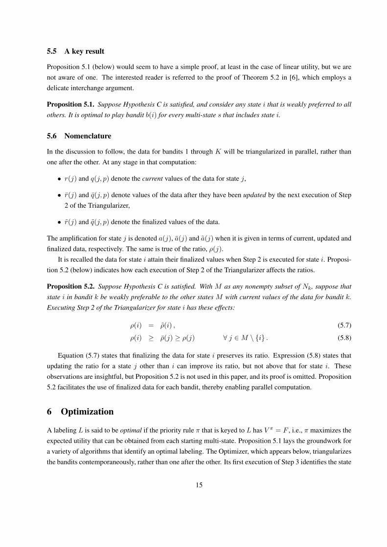
5.5 A key result

Proposition 5.1 (below) would seem to have a simple proof, at least in the case of linear utility, but we arenot aware of one. The interested reader is referred to the proof of Theorem 5.2 in [6], which employs adelicate interchange argument.

Proposition 5.1. Suppose Hypothesis C is satisfied, and consider any state i that is weakly preferred to allothers. It is optimal to play bandit b(i) for every multi-state s that includes state i.

5.6 Nomenclature

In the discussion to follow, the data for bandits 1 through K will be triangularized in parallel, rather thanone after the other. At any stage in that computation:

• r(j) and q(j, p) denote the current values of the data for state j,

• r(j) and q(j, p) denote values of the data after they have been updated by the next execution of Step2 of the Triangularizer,

• r(j) and q(j, p) denote the finalized values of the data.

The amplification for state j is denoted a(j), a(j) and a(j) when it is given in terms of current, updated andfinalized data, respectively. The same is true of the ratio, ρ(j).

It is recalled the data for state i attain their finalized values when Step 2 is executed for state i. Proposi-tion 5.2 (below) indicates how each execution of Step 2 of the Triangularizer affects the ratios.

Proposition 5.2. Suppose Hypothesis C is satisfied. With M as any nonempty subset of Nk, suppose thatstate i in bandit k be weakly preferable to the other states M with current values of the data for bandit k.Executing Step 2 of the Triangularizer for state i has these effects:

ρ(i) = ρ(i) , (5.7)

ρ(i) ≥ ρ(j) ≥ ρ(j) ∀ j ∈M \ {i} . (5.8)

Equation (5.7) states that finalizing the data for state i preserves its ratio. Expression (5.8) states thatupdating the ratio for a state j other than i can improve its ratio, but not above that for state i. Theseobservations are insightful, but Proposition 5.2 is not used in this paper, and its proof is omitted. Proposition5.2 facilitates the use of finalized data for each bandit, thereby enabling parallel computation.

6 Optimization

A labeling L is said to be optimal if the priority rule π that is keyed to L has V π = F , i.e., π maximizes theexpected utility that can be obtained from each starting multi-state. Proposition 5.1 lays the groundwork fora variety of algorithms that identify an optimal labeling. The Optimizer, which appears below, triangularizesthe bandits contemporaneously, rather than one after the other. Its first execution of Step 3 identifies the state

15

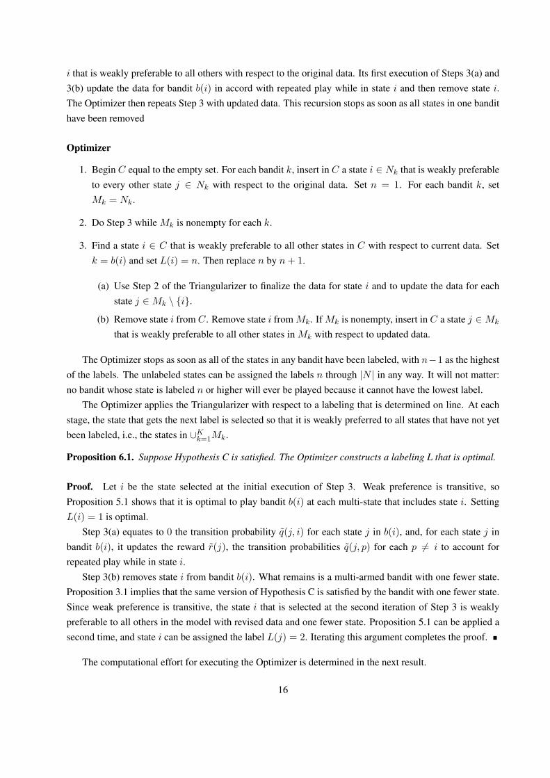
i that is weakly preferable to all others with respect to the original data. Its first execution of Steps 3(a) and3(b) update the data for bandit b(i) in accord with repeated play while in state i and then remove state i.The Optimizer then repeats Step 3 with updated data. This recursion stops as soon as all states in one bandithave been removed

Optimizer

1. Begin C equal to the empty set. For each bandit k, insert in C a state i ∈ Nk that is weakly preferableto every other state j ∈ Nk with respect to the original data. Set n = 1. For each bandit k, setMk = Nk.

2. Do Step 3 while Mk is nonempty for each k.

3. Find a state i ∈ C that is weakly preferable to all other states in C with respect to current data. Setk = b(i) and set L(i) = n. Then replace n by n+ 1.

(a) Use Step 2 of the Triangularizer to finalize the data for state i and to update the data for eachstate j ∈Mk \ {i}.

(b) Remove state i from C. Remove state i from Mk. If Mk is nonempty, insert in C a state j ∈Mk

that is weakly preferable to all other states in Mk with respect to updated data.

The Optimizer stops as soon as all of the states in any bandit have been labeled, with n−1 as the highestof the labels. The unlabeled states can be assigned the labels n through |N | in any way. It will not matter:no bandit whose state is labeled n or higher will ever be played because it cannot have the lowest label.

The Optimizer applies the Triangularizer with respect to a labeling that is determined on line. At eachstage, the state that gets the next label is selected so that it is weakly preferred to all states that have not yetbeen labeled, i.e., the states in ∪Kk=1Mk.

Proposition 6.1. Suppose Hypothesis C is satisfied. The Optimizer constructs a labeling L that is optimal.

Proof. Let i be the state selected at the initial execution of Step 3. Weak preference is transitive, soProposition 5.1 shows that it is optimal to play bandit b(i) at each multi-state that includes state i. SettingL(i) = 1 is optimal.

Step 3(a) equates to 0 the transition probability q(j, i) for each state j in b(i), and, for each state j inbandit b(i), it updates the reward r(j), the transition probabilities q(j, p) for each p = i to account forrepeated play while in state i.

Step 3(b) removes state i from bandit b(i). What remains is a multi-armed bandit with one fewer state.Proposition 3.1 implies that the same version of Hypothesis C is satisfied by the bandit with one fewer state.Since weak preference is transitive, the state i that is selected at the second iteration of Step 3 is weaklypreferable to all others in the model with revised data and one fewer state. Proposition 5.1 can be applied asecond time, and state i can be assigned the label L(j) = 2. Iterating this argument completes the proof.

The computational effort for executing the Optimizer is determined in the next result.

16

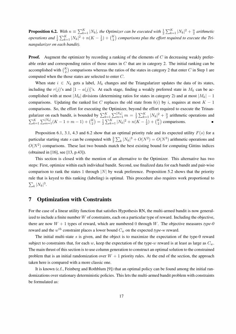
Proposition 6.2. With n ≡∑K

k=1 |Nk|, the Optimizer can be executed with 12

∑Kk=1 |Nk|2 + n

2 arithmeticoperations and 1

2

∑Kk=1 |Nk|2 + n(K − 1

2) +(K2

)comparisons plus the effort required to execute the Tri-

nangularizer on each bandit).

Proof. Augment the optimizer by recording a ranking of the elements of C in decreasing weakly prefer-able order and corresponding ratios of those states in C that are in category 2. The initial ranking can beaccomplished with

(K2

)comparisons whereas the ratios of the states in category 2 that enter C in Step 1 are

computed when the those states are selected to enter C.When state i ∈ Nk gets a label, Mk changes and the Triangularizer updates the data of its states,

including the r(j)’s and [1 − a(j)]’s. At each stage, finding a weakly preferred state in Mk can be ac-complished with at most |Mk| divisions (determining ratios for states in category 2) and at most |Mk| − 1

comparisons. Updating the ranked list C replaces the old state from b(i) by i, requires at most K − 1

comparisons. So, the effort for executing the Optimizer, beyond the effort required to execute the Trinan-gularizer on each bandit, is bounded by

∑Kk=1

∑|Nk|m=1m = 1

2

∑Kk=1 |Nk|2 + n

2 arithmetic operations and∑Kk=1

∑|Nk|m=1(K − 1 +m− 1) +

(K2

)= 1

2

∑Kk=1 |Nk|2 + n(K − 1

2) +(K2

)comparisons.

Proposition 6.1, 3.1, 4.3 and 6.2 show that an optimal priority rule and its expected utility F (s) for aparticular starting state s can be computed with 3

2

∑k |Nk|3 + O(N2) = O(N3) arithmetic operations and

O(N2) comparisons. These last two bounds match the best existing bound for computing Gittins indices(obtained in [16], see [13, p.43]).

This section is closed with the mention of an alternative to the Optimizer. This alternative has twosteps: First, optimize within each individual bandit. Second, use finalized data for each bandit and pair-wisecomparison to rank the states 1 through |N | by weak preference. Proposition 5.2 shows that the priorityrule that is keyed to this ranking (labeling) is optimal. This procedure also requires work proportional to∑

k |Nk|3.

7 Optimization with Constraints

For the case of a linear utility function that satisfies Hypothesis RN, the multi-armed bandit is now general-ized to include a finite number W of constraints, each on a particular type of reward. Including the objective,there are now W + 1 types of reward, which are numbered 0 through W . The objective measures type-0reward and the wth constraint places a lower bound Cw on the expected type-w reward.

The initial multi-state s is given, and the object is to maximize the expectation of the type-0 rewardsubject to constraints that, for each w, keep the expectation of the type-w reward is at least as large as Cw.The main thrust of this section is to use column generation to construct an optimal solution to the constrainedproblem that is an initial randomization over W + 1 priority rules. At the end of the section, the approachtaken here is compared with a more classic one.

It is known (c.f., Feinberg and Rothblum [9]) that an optimal policy can be found among the initial ran-domizations over stationary deterministic policies. This lets the multi-armed bandit problem with constraintsbe formulated as:

17

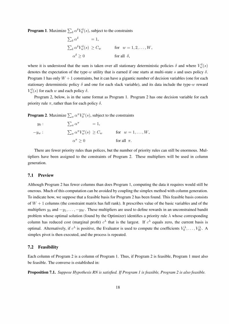
Program 1. Maximize∑

δ αδV δ

0 (s), subject to the constraints∑δ α

δ = 1,∑δ α

δV δw(s) ≥ Cw for w = 1, 2, . . . ,W ,

αδ ≥ 0 for all δ,

where it is understood that the sum is taken over all stationary deterministic policies δ and where V δw(s)

denotes the expectation of the type-w utility that is earned if one starts at multi-state s and uses policy δ.Program 1 has only W +1 constraints, but it can have a gigantic number of decision variables (one for eachstationary deterministic policy δ and one for each slack variable), and its data include the type-w rewardV δw(s) for each w and each policy δ.

Program 2, below, is in the same format as Program 1. Program 2 has one decision variable for eachpriority rule π, rather than for each policy δ.

Program 2. Maximize∑

π απV π

0 (s), subject to the constraints

y0 :∑

π απ = 1,

−yw :∑

π απV π

w (s) ≥ Cw for w = 1, . . . ,W ,

απ ≥ 0 for all π.

There are fewer priority rules than polices, but the number of priority rules can still be enormous. Mul-tipliers have been assigned to the constraints of Program 2. These multipliers will be used in columngeneration.

7.1 Preview

Although Program 2 has fewer columns than does Program 1, computing the data it requires would still beonerous. Much of this computation can be avoided by coupling the simplex method with column generation.To indicate how, we suppose that a feasible basis for Program 2 has been found. This feasible basis consistsof W + 1 columns (the constraint matrix has full rank). It prescribes value of the basic variables and of themultipliers y0 and −y1, . . . ,−yW . These multipliers are used to define rewards in an unconstrained banditproblem whose optimal solution (found by the Optimizer) identifies a priority rule λ whose correspondingcolumn has reduced cost (marginal profit) cλ that is the largest. If cλ equals zero, the current basis isoptimal. Alternatively, if cλ is positive, the Evaluator is used to compute the coefficients V λ

0 , . . . , V λW . A

simplex pivot is then executed, and the process is repeated.

7.2 Feasibility

Each column of Program 2 is a column of Program 1. Thus, if Program 2 is feasible, Program 1 must alsobe feasible. The converse is established in:

Proposition 7.1. Suppose Hypothesis RN is satisfied. If Program 1 is feasible, Program 2 is also feasible.

18

Proof. We will prove the contrapositive. Suppose that Program 2 is not feasible. An application of Farkas’lemma (equivalently of the duality theorem of linear programming) shows that there exist numbers y0 andy1 through yw such that

y0 −W∑w=1

ywVπw (s) ≥ 0 for all π , (7.1)

yw ≥ 0 for w = 1, . . . ,W , (7.2)

y0 −W∑w=1

ywCw < 0 . (7.3)

The numbers y1 through yW will be used as weights for the rewards r1(i) through rW (i). Consideran unconstrained multi-armed bandit in which the reward R(i) for playing bandit b(i) while its state is i isgiven by R(i) = y1r1(i) + · · · + yW rW (i). Expression (7.1) states that with reward R(i) for each state i,no priority rule π has aggregate reward that exceeds y0. Proposition 5.1 shows that a priority rule is optimal.Thus,

y0 −W∑w=1

ywVδw(s) ≥ 0 for all δ . (7.4)

where δ ranges over all stationary deterministic policies. A solution exists to (7.2)–(7.4), so a second appli-cation of Farkas’ lemma shows that no solution exists to the constraints of Program 1.

Thus, Program 1 is feasible if and only if Program 2 is feasible. Phase I of the simplex method will besoon used to determine whether Program 2 is feasible and, if so, to construct a feasible basis with which toinitiate Phase II of the simplex method. For the moment, it is assumed that a feasible basis for Program 2has been found.

7.3 Phase II

The constraint matrix for Program 2 includes a column for each of the W slack variables. These columnsare linearly independent of each other, and they are linearly independent of the other columns. Thus, therank of its constraint matrix equals the number W + 1 of its rows, and each basis for Program 2 consists ofexactly W + 1 columns. Let us consider an iteration of Phase II. At hand at the start of this iteration is afeasible basis, its basic solution and its multipliers. This information includes:

• The data (column) for each of the W + 1 basic variables.

• The basic solution (the απ’s) for this basis.

• The multipliers y0 and y1 through yW for this basis.

The multipliers y1 through yW are nonnegative, and each priority rule λ has reduced cost cλ that is given by

cλ = V λ0 (s) +

W∑w=1

ywVλw (s)− y0 .

19

Computation of the reduced cost of each nonbasic priority rule λ would be an onerous task, but it is notnecessary. To determine whether or not the current basis is optimal and, if not, to find a priority rule has thelargest (most positive) reduced cost, one can solve the unconstrained multi-armed bandit problem with thereward R(i) for playing bandit b(i) when its state is i given by

R(i) = r0(i) +W∑w=1

ywrw(i) . (7.5)

With these rewards, the Optimizer in Section 7 computes a priority rule π that is optimal. Also, theEvaluator in Section 5 computes the expected return V π(s) for starting in multi-state s and using this priorityrule. If V π(s) ≤ y0, no nonbasic variable has a positive reduced cost, so the current basis is optimal.If V π(s) > y0, the column for priority rule π enters the basis. To compute V π

w (s) for each w, use theTriangularizer and Evaluator for priority rule π. In this computation, the finalized rewards vary with w butthe yk(j)’s do not. To complete an iteration of Phase II, execute a feasible pivot with απ as the enteringvariable.

7.4 Phase II recap

Each feasible basis and its basic solution prescribe an initial randomization (with weight απ assigned topriority rule π) over (W +1− p) priority rules, where p equals the number of slack variables that are basic.

The multipliers for the current basis determine the data of an unconstrained bandit problem, and theprocedure in prior sections computes its optimal priority rule π and its expected return, V π(s). If V π(s)

does not exceed y0, the current basis is optimal. If V π(s) exceeds y0, the Evaluator is used to compute thecoefficients V π

0 through V πW of the entering variable. A simplex pivot is then executed.

The pivot itself requires work proportional to (W +1)3. Identifying the entering variable and its columnof coefficients entails work proportional to (W +2)[

∑k |Nk|3]. Only a few iterations may be needed to find

a good basis, or an optimal basis, but that is not guaranteed.

7.5 Phase I

It remains to determine whether or not Program 2 is feasible and, if it is feasible, to construct a feasiblebasis with which to initiate Phase II. These tasks will be accomplished by “bringing in” the constraints ofProgram 2, one at a time. Starting with n = 1, the nth iteration of Phase I is initialized with a randomizationover n− 1 priority rules that satisfy the first n− 1 constraints. The nth iteration maximizes type-n reward,using the Phase II column generation scheme described above. If the type-n income can be made as largeas Cn, a basis has been found with which to initiate the n + 1st iteration. If not, no feasible solution existsto Program 2.

7.6 The classic formulation

An optimal policy for a discounted Markov decision problem with W constraints can be found among thestationary randomized policies (c.f., Altman [1, page 102]). This can be accomplished by a linear program

20

whose constraint matrix has one column per state-action pair, one row per state, and one row per constraint.The multi-armed bandit has J =

∏Kk=1 |Nk|multi-states and K actions per multi-state. Its constraint matrix

has W + J rows and K × J columns. The classic formulation has fewer columns than does Program 2, butit has many more rows.

The classic formulation can also be attacked by column generation, but doing so would be unattractivebecause the formulation would have more columns and many more rows than the one we propose.

7.7 A roadblock

With a linear utility function, multiple types of reward can be handled by column generation and by theclassic method. Both methods utilize the fact that each transition rate q(i, j) is independent of the rewardtype.

Let us consider what occurs when multiple types of rewards are introduced in the model with exponentialutility. Note from (2.4) and (2.5) that the payoff x(i, j) appears in the formula for the transition rate q(i, j).Having multiple types of income causes the transition rate q(i, j) to vary with the reward type. Consequently,our column generation method (and the classical one) can be applied only when the type-w payoff xw(i, j)is independent of w, for instance, this is the case when income is earned only at termination.

8 Structural properties

In the prior section, it was demonstrated that an optimal policy for a constrained bandit problem can befound among the initial randomization over W +1 priority rules. In the current section, the structure of thisoptimal policy is probed.

A transient Markov decision problem (MDP) with W constraints has an optimal solution that is an initialrandomization over W + 1 deterministic policies δ1 through δW+1 each of which differs from the next atprecisely one state of the MDP; see Feinberg and Rothblum [9]. When this MDP is a multi-armed bandit,these deterministic policies need not be priority rules, however.

Two labelings are now said to be adjacent if they are identical except that they exchange the stateshaving labels k and k+1 for exactly one value of k. The aforementioned property raises the question: DoesProgram 2 have an optimal solution that is an initial randomization over priority rules that are keyed to asequence of W + 1 labelings with the property that each labeling is adjacent to the next? This question willbe answered in the affirmative in the case of one constraint and in the negative in the case of more than oneconstraint.

8.1 Adjacency with one constraint

Let us consider a multi-armed bandit with one constraint. We have seen that an optimal basis for Program 2prescribes a randomization over at most two priority rules. If its basic solution for this basis sets αj = 1 forany j, only priority rule is used, and adjacency is trivial.

Let us denote as V p0 and V p

1 as the type-0 and type-1 utility for column p. The case that requires analysisis that in which the optimal basis for Program 2 consists of columns j and k whose priority rules are keyed

21

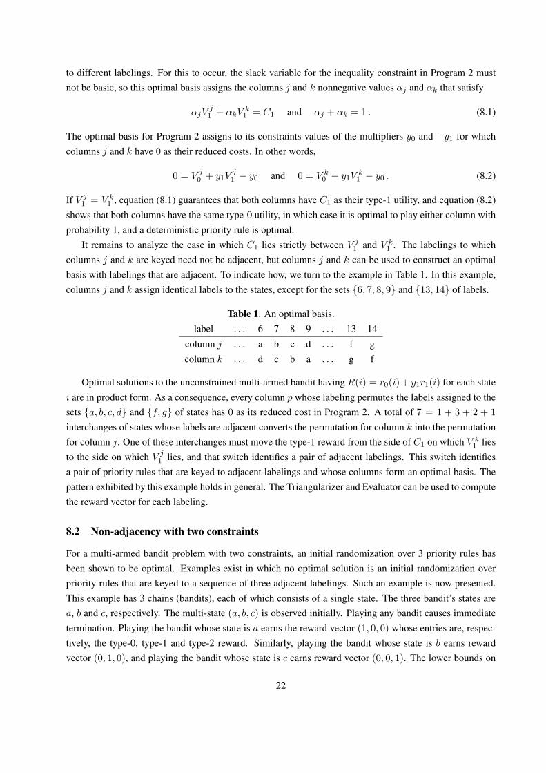
to different labelings. For this to occur, the slack variable for the inequality constraint in Program 2 mustnot be basic, so this optimal basis assigns the columns j and k nonnegative values αj and αk that satisfy

αjVj1 + αkV

k1 = C1 and αj + αk = 1 . (8.1)

The optimal basis for Program 2 assigns to its constraints values of the multipliers y0 and −y1 for whichcolumns j and k have 0 as their reduced costs. In other words,

0 = V j0 + y1V

j1 − y0 and 0 = V k

0 + y1Vk1 − y0 . (8.2)

If V j1 = V k

1 , equation (8.1) guarantees that both columns have C1 as their type-1 utility, and equation (8.2)shows that both columns have the same type-0 utility, in which case it is optimal to play either column withprobability 1, and a deterministic priority rule is optimal.

It remains to analyze the case in which C1 lies strictly between V j1 and V k

1 . The labelings to whichcolumns j and k are keyed need not be adjacent, but columns j and k can be used to construct an optimalbasis with labelings that are adjacent. To indicate how, we turn to the example in Table 1. In this example,columns j and k assign identical labels to the states, except for the sets {6, 7, 8, 9} and {13, 14} of labels.

Table 1. An optimal basis.label . . . 6 7 8 9 . . . 13 14

column j . . . a b c d . . . f gcolumn k . . . d c b a . . . g f

Optimal solutions to the unconstrained multi-armed bandit having R(i) = r0(i)+ y1r1(i) for each statei are in product form. As a consequence, every column p whose labeling permutes the labels assigned to thesets {a, b, c, d} and {f, g} of states has 0 as its reduced cost in Program 2. A total of 7 = 1 + 3 + 2 + 1

interchanges of states whose labels are adjacent converts the permutation for column k into the permutationfor column j. One of these interchanges must move the type-1 reward from the side of C1 on which V k

1 liesto the side on which V j

1 lies, and that switch identifies a pair of adjacent labelings. This switch identifiesa pair of priority rules that are keyed to adjacent labelings and whose columns form an optimal basis. Thepattern exhibited by this example holds in general. The Triangularizer and Evaluator can be used to computethe reward vector for each labeling.

8.2 Non-adjacency with two constraints

For a multi-armed bandit problem with two constraints, an initial randomization over 3 priority rules hasbeen shown to be optimal. Examples exist in which no optimal solution is an initial randomization overpriority rules that are keyed to a sequence of three adjacent labelings. Such an example is now presented.This example has 3 chains (bandits), each of which consists of a single state. The three bandit’s states area, b and c, respectively. The multi-state (a, b, c) is observed initially. Playing any bandit causes immediatetermination. Playing the bandit whose state is a earns the reward vector (1, 0, 0) whose entries are, respec-tively, the type-0, type-1 and type-2 reward. Similarly, playing the bandit whose state is b earns rewardvector (0, 1, 0), and playing the bandit whose state is c earns reward vector (0, 0, 1). The lower bounds on

22

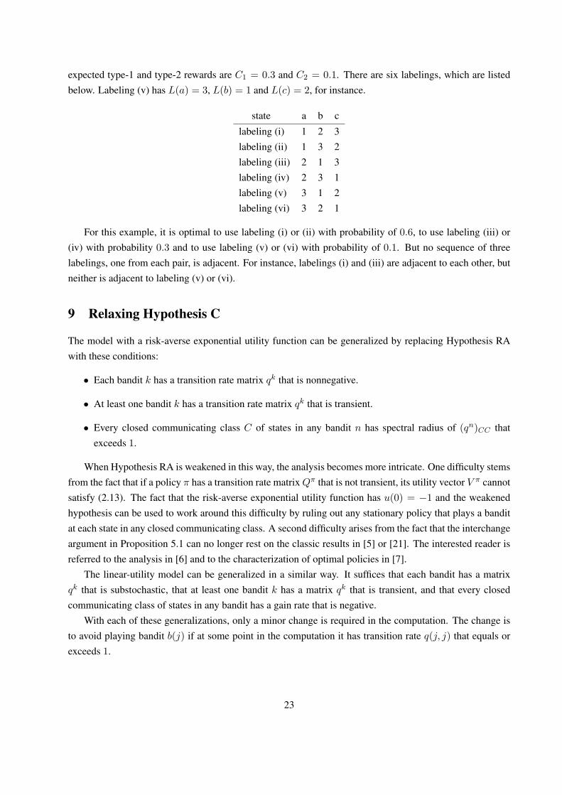
expected type-1 and type-2 rewards are C1 = 0.3 and C2 = 0.1. There are six labelings, which are listedbelow. Labeling (v) has L(a) = 3, L(b) = 1 and L(c) = 2, for instance.

state a b c

labeling (i) 1 2 3labeling (ii) 1 3 2labeling (iii) 2 1 3labeling (iv) 2 3 1labeling (v) 3 1 2labeling (vi) 3 2 1

For this example, it is optimal to use labeling (i) or (ii) with probability of 0.6, to use labeling (iii) or(iv) with probability 0.3 and to use labeling (v) or (vi) with probability of 0.1. But no sequence of threelabelings, one from each pair, is adjacent. For instance, labelings (i) and (iii) are adjacent to each other, butneither is adjacent to labeling (v) or (vi).

9 Relaxing Hypothesis C

The model with a risk-averse exponential utility function can be generalized by replacing Hypothesis RAwith these conditions:

• Each bandit k has a transition rate matrix qk that is nonnegative.

• At least one bandit k has a transition rate matrix qk that is transient.

• Every closed communicating class C of states in any bandit n has spectral radius of (qn)CC thatexceeds 1.

When Hypothesis RA is weakened in this way, the analysis becomes more intricate. One difficulty stemsfrom the fact that if a policy π has a transition rate matrix Qπ that is not transient, its utility vector V π cannotsatisfy (2.13). The fact that the risk-averse exponential utility function has u(0) = −1 and the weakenedhypothesis can be used to work around this difficulty by ruling out any stationary policy that plays a banditat each state in any closed communicating class. A second difficulty arises from the fact that the interchangeargument in Proposition 5.1 can no longer rest on the classic results in [5] or [21]. The interested reader isreferred to the analysis in [6] and to the characterization of optimal policies in [7].

The linear-utility model can be generalized in a similar way. It suffices that each bandit has a matrixqk that is substochastic, that at least one bandit k has a matrix qk that is transient, and that every closedcommunicating class of states in any bandit has a gain rate that is negative.

With each of these generalizations, only a minor change is required in the computation. The change isto avoid playing bandit b(j) if at some point in the computation it has transition rate q(j, j) that equals orexceeds 1.

23

10 Acknowledgements

The authors are pleased to acknowledge that this paper has benefited immensely from the reactions of Dr.Pelin Cambolat to earlier drafts. The contribution of the second author has been supported in part by NSFgrant CMMI-0928490. The contribution of the third author has been supported in part by ISF Israel ScienceFoundation) grant 901/10.

References

[1] Altman, E. 1999. Constrained Markov Decision Processes. Chapman & Hall/CRC, Boca Raton, USA.

[2] Bergemann, D., J. Valimakim. 2008. Bandit problems. S. Durlauf, L. Blume, eds. The New PalgraveDictionary of Economics (2nd edition).

[3] Berry, D. A., B. Friestedt. 1985. Bandit Problems. Chapman Hall.

[4] Bertsimas, D., J. Nino-Mora. 1993. Conservation laws, extended polymatroids and multi-armed banditproblems: a polyhedral approach to indexable systems. Mathematics of Operations Research 21, 257–306.

[5] Denardo, E.V. 1967. Contraction mappings in the theory underlying dynamic programming. SIAMReview 9, 165–177.

[6] Denardo, E.V., H. Park, U.G. Rothblum. 2007. Risk-sensitive and risk-neutral multiarmed bandits.Mathematics of Operations Research 32, 374–394.

[7] Denardo, E.V., U.G. Rothblum. 2006. A turnpike theorem for a risk-sensitive Markov decision problemwith stopping. SIAM J. Control Optim. 45, 414–431.

[8] El Karoui, N., I. Karatzas. 1994. Dynamic allocation indices in continuous time. Annals of AppliedProbability 4, 255–286.

[9] Feinberg, E.A., U.G. Rothblum. 2011. Splitting randomized stationary policies in total-reward Markovdecision processes. Mathematics of Operations Research, to appear.

[10] Gittins, J.C. 1979. Bandit problems and dynamic allocation indices (with discussion). Journal of theRoyal Statistical Society B. 41, 148-177.

[11] Gittins, J.C. 1989. Multi-armed bandit allocation indices. John Wiley and Sons Inc.

[12] Gittins, J.C., D.M. Jones. 1974. A dynamic allocation index for the sequential design experiments.J. Gani, K. Sarkadu, I. Vince, eds. Progress in Statistics, European Meeting of Statisticians I, NorthHolland, Amsterdam, 241–266.

[13] Gittins, J.C., K. Glazebrook, R. Weber. 2011. Multi-armed bandit allocation indices (2nd edition). JohnWiley and Sons Inc.

[14] Kaspi, H., A. Mandelbaum. 1998. Multi-armed bandits in discrete and continuous time. Annals ofApplied Probability 8, 1270–1290.

24

[15] Katehakis, M., A.F. Veinott, Jr. 1987. The multiarmed bandit problem: Decomposition and computa-tion. Mathematics of Operations Research 22, 262–268.

[16] Nino-Mora, J. 2007. A (2/3)n3 fast pivoting algorithm for the Gittins index and optimal stopping of aMarkov chain. INFORMS Journal on Computing 10, 596–606.

[17] Schlag, K. 1998. Why imitate, and if so, how? A bounded rational approach to multi-armed bandits.Journal of Economic Theory 78, 130–156.

[18] Sonin, I. 2008. A generalized Gittins index for Markov chains and its recursive calculation. TechnicalReport. Statistics and Probability Letters 78, 1526–1533.

[19] Tsitsiklis, J. 1994. A short proof of the Gittins index theorem. Annals of Applied Probability 4, 194–199.

[20] Variaya, P., J. Walrand, C. Buyukkoc. 1985. Extensions of the multi-armed bandit problem: The dis-counted case. IEEE Trans. Automat. Control AC-30, 426–439.

[21] Veinott, A.F., Jr. 1969. Discrete dynamic programming with sensitive discount optimality criteria. Ann.Math. Statist. 40, 1635–1660.

[22] Weber, R. 1992. On the Gittins index for multiarmed bandits. Annals of Applied Probability 2, 1024–1033.

[23] Weiss, G. 1988. Branching bandit processes. Probability in the Engineering and Informational Sciences2, 269–278.

[24] Whittle, P. 1980. Multi-armed bandits and the Gittins index. J. Roy. Statist. Soc. B 43, 143–149.

25