1

Multi-criteria risk assessment approach for components risk

ranking– The case study of an offshore Wave Energy Converter

Uzoma Okoro*, Athanasios Kolios 1*, Lin Cui+

*Centre for Offshore Renewable Energy Engineering, School of Energy, Environment and Agrifood,

Cranfield University, Cranfield, MK43 0AL, UK

+National Ocean Technology Centre, Tianjin, China

Abstract

Experts’ judgement is employed in offshore risk assessment because reliable failure data for

quantitative risk analysis are scarce. The challenges with this practice lies with knowledge-

based uncertainties which renders risk expression and estimation, hence components’ risk-

based prioritisation, subjective to the assessor – even for the same case study. In this paper, a

new risk assessment framework is developed to improve the fidelity and consistency of

prioritisation of components of complex offshore engineering systems based on expert

judgement. Unlike other frameworks, such as the Failure Mode and Effect Criticality

Analysis, it introduces two additional dimensions: variables and parameters, to allow more

effective scoring. These additional dimensions provide the much needed and uniform

information that will assist experts with the estimation of probability of occurrence, severity

of consequence and safeguards, herein referred to as 3-D methodology. In so doing, it

achieves a more systematic approach to risk description and estimation compared to the

conventional Risk Priority Number (RPN) of FMECA. Finally, the framework is

demonstrated on a real case study of a wave energy converter (WEC) and conclusions of the

assessment proved well in comparison and prioritization.

Keywords: Condition-based risk assessment, risk estimation, multi-criteria risk assessment,

wave energy converter.

1 Corresponding author. Tel.: +44 (0) 1234 754631; E-mail address: a.kolios@cranfield.ac.uk

2

1. Introduction

The establishment of effective safety routines ensures extended and efficient operations,

increasing production and lowering levelized cost of energy (LCOE), and consequently

increasing the competitive advantage of operators. Defined as “…the ratio of the total cost of

the power source to the total energy output over its life…” LCOE forms a commonly used

metric to compare the costs of various energy generation technologies. Considering that

Capital Expenditure (CAPEX) is distributed over a larger production output, as a result of

more efficient management lower LCOE holds the key to a significant increase in return on

investment (ROI).

Generally, cost of safety processes such as Inspection, Repair and Maintenance (IRM) for

offshore energy structures is abysmally high compared to those in onshore locations. An

effective maintenance plan deploys the limited resources to target the most urgent failure

modes [1,2] but such decision-making is difficult as it is hard to predict what would be the

consequences of a decision, especially when it involves high risk and large uncertainties [3].

It is in this context that risk analysis is adopted as an essential decision support tool to

anticipate all the uncertainties, study the likely outcome and take a guided decision. Risk

analysis techniques identify the possible sources of hazards and quantify/estimate the

attributes of likelihood of occurrence, consequence and possibility of detection [4]. The

challenge of risk analysis approaches for use as a decision support tool lies in the detail to

which it is capable of considering risk contributory factors, the clarity of risk expression and

risk-level estimation [5], and the procedure for risk comparison. In situations where there is

lack of accurate failure data for use in quantitative analysis, these descriptions are carried out

qualitatively by experts who draw from a wealth of long standing experience and common

sense in the subject matter to make judgements. However, these judgements suffer linguistic,

lexical and informal uncertainties [6,7] such that analyses’ conclusions are subjective to the

expert and incomparable [8].

Amongst the various solutions proposed by different authors [1,9–11], FMEA is the most

widely practised [12–19]. FMEA’s simplified semi-quantitative framework possesses the

combined advantages of quantitative and qualitative features it uses to describe the risk

criteria; Occurrence (O), Severity (S) of the effect and Failure detection (D), and integrates

them on a multiplicative scale to give a single-point measure of risk ranking as shown in (1).

3

However, use of FMEA is not without its own criticisms. In fact in [20,21], O, S, and D are

classified as high (system)-level evaluation criteria, i.e., ones that give low-levels of detail,

and end up in top-level estimates of risk level. Such analysis will lead to results that are not

only highly subjective but also non-repeatable [8]. Risk level estimation based on

Multiplicative aggregation models, such as found in Risk Priority Number (RPN), are also

criticised in [6], as always giving an inconsistent variance of risk scores. Still on RPN, [22]

raises questions on a number of issues, such as – i) the use of the ordinal ranking numbers as

numeric quantities (i.e., referring to multiplication), ii) the presence of “holes” constituting a

large part of the RPN measurement scale, iii) duplicate RPN values with very different

combinations of O, S and D scores, and iv) the high sensitivity to small changes. Figure 1

shows the plot of RPN against frequency of a random combination of O, S and D. Holes are

shown as portions of discontinuities between successive RPNs in multiplicative scales. The

direct consequence of ‘sensitivity to small changes’ is that errors due to uncertainties

associated with the judgement of O, S and D becomes exaggerated. This is demonstrated in

(2) and (3). As can be seen in each of the parentheses of (3), the errors in judgement of O, S

and D, denoted as o , s and d respectively, are exaggerated when multiplied. These make

FMEA analysis results non-repeatable and subjective, and their interpretation problematic.

[( ) ( ) ( )]RPN O o S s D d O S D (2)

( ) ( ) ( )

( ) ( ) ( )

RPN S o D s O D s o D

S O d S o d s O d

(3)

Figure 1 Holes shown in Frequency versus RPN plot

0 100 200 300 400 500 600 700 800 900 10000

5

10

15

20

25

RPN Value

Num

ber

of

Occ

urr

ence

A hole

Fre

quen

cy o

f O

ccurr

ence

RPN Value

( )i iRPN O S D (1)

4

This paper develops a framework for prioritising components of offshore structures based on

estimated risk level as a decision support for resource allocation or other forms of

intervention action. Because there will always be more failure modes to mitigate than there

are resources available, this makes the framework a cost-effective risk management tool. The

basic assumptions of the proposed framework are that: a) risk exposure is a listing of failure

modes, variables and parameters, b) the components are exposed differently to different risk

sources, c) failure results from a combination of the listed failure modes/mechanism, and d)

that any two or more assessors given detailed information on the conditions of exposures will

arrive at the same conclusions on frequency of failure, severity of consequence and

“provision of safe guards” for each component.

The above assumptions are actually part of the rationale behind the model. Most known risk

analysis method follow this assumption of finite listing of failure modes/mechanisms,

variables and parameters, whereas in reality, the listing is infinite. This is one of the

shortcoming of risk analysis ideology as a whole because it is not the known failure

modes/mechanisms, variables and parameters that is the problem, but rather the unknown

ones. This is why continuous study of risk is encouraged. The second assumption describes

the structure of the model to accommodate cases where the components are exposed to the

same risk. In such case the performance scores of the components under the rest of risk

sources not considered is set at zero. The third assumption sets the limits of the methodology

to generic failure modes/mechanisms highlighting that not-known risks should also be

included in the analysis through following a similar rationale as the one developed for the

generic ones. Finally, reproducibility of the methodology is a key enabler of this method as it

allows to overcome some of the key barriers of traditional risk assessment methods.

Efforts are concerted on achieving a more systematic expression/description and estimation

of risk for different components under different failure modes/mechanisms. Though

expressions of risk description and estimation broken down to low-levels of detail make risk

assessment and decision making process cumbersome, however, it further helps clear areas of

uncertainty and most importantly provides documented evidence for arriving at operational

decisions, thus reducing errors due to subjectivity. It is in this context that Multi-Criteria

Decision Analysis (MCDA) is often employed to handle issues of incomplete information

and to facilitate systemic understanding. As part of the required analytical steps, the elicited

scores, with parameters’ weight are aggregated to derive an index for rank-ordering. These

5

are demonstrated on the real case study of a wave energy converter (WEC). Furthermore, the

concept of Safeguard is introduced (expanding the concept of Detection in FMEA) to

represent existing failure mitigating measures, recognising the fact that the extent of risk due

to a specific failure mechanism is dependent on the availability and efficiency of relevant

safeguards.

2.0 A Framework for Condition-based Risk assessment model

2.1 Understanding risk

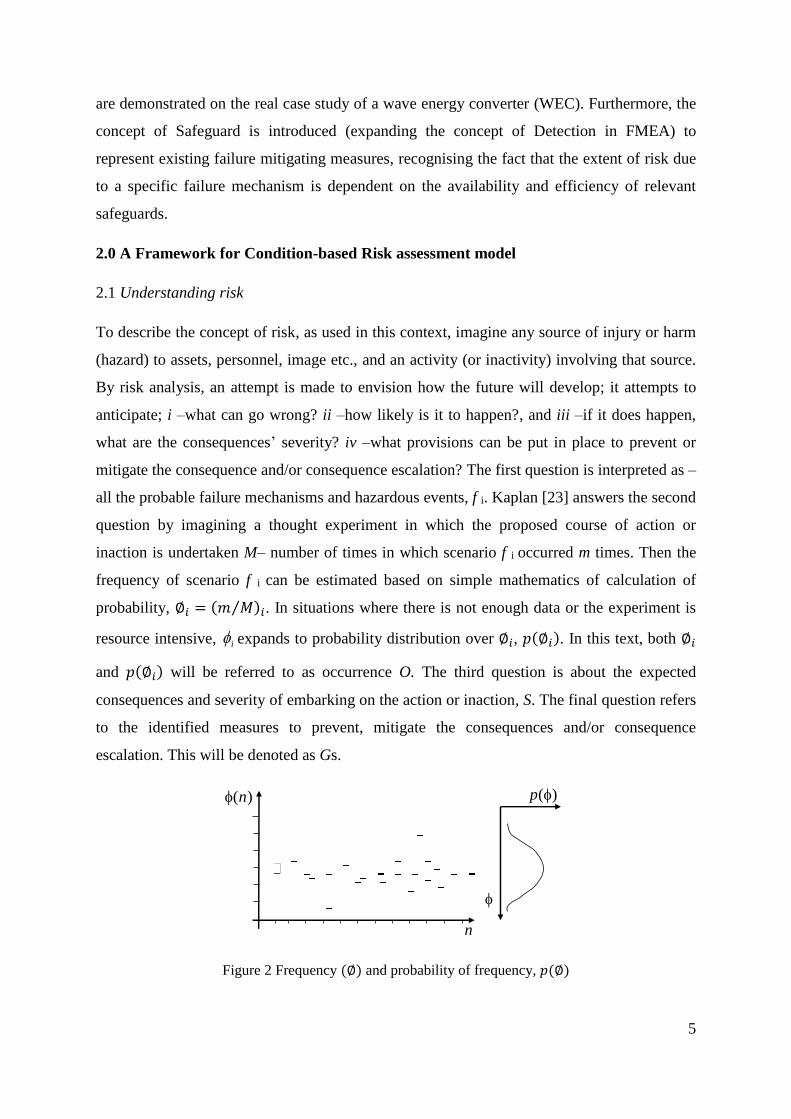
To describe the concept of risk, as used in this context, imagine any source of injury or harm

(hazard) to assets, personnel, image etc., and an activity (or inactivity) involving that source.

By risk analysis, an attempt is made to envision how the future will develop; it attempts to

anticipate; i –what can go wrong? ii –how likely is it to happen?, and iii –if it does happen,

what are the consequences’ severity? iv –what provisions can be put in place to prevent or

mitigate the consequence and/or consequence escalation? The first question is interpreted as –

all the probable failure mechanisms and hazardous events, f i. Kaplan [23] answers the second

question by imagining a thought experiment in which the proposed course of action or

inaction is undertaken M– number of times in which scenario f i occurred m times. Then the

frequency of scenario f i can be estimated based on simple mathematics of calculation of

probability, ∅𝑖 = (𝑚 𝑀⁄ )𝑖. In situations where there is not enough data or the experiment is

resource intensive, i expands to probability distribution over ∅𝑖, 𝑝(∅𝑖). In this text, both ∅𝑖

and 𝑝(∅𝑖) will be referred to as occurrence O. The third question is about the expected

consequences and severity of embarking on the action or inaction, S. The final question refers

to the identified measures to prevent, mitigate the consequences and/or consequence

escalation. This will be denoted as Gs.

Figure 2 Frequency (∅) and probability of frequency, 𝑝(∅)

( )n

( )p

n

6

Complete answers to these questions will contain a set of all the scenarios, probability of

frequency (or just frequency) and measures of damages as well as safeguards as shown in (4).

This is referred to as risk.

1 1 1 1

2 2 2 2

i i i i

N N N N

f O S G

f O S G

Rf O S G

f O S G

(4)

2.2 Description of Framework

The methodology proposed in this paper fundamentally consists of elements of risk

assessment i.e., identification, analysis and evaluation of hazard sources [4]. The contribution

is the systematic approach, depth of analysis and complexity of the systems to which the

method is being applied. The framework shares some common features with FMEA in that

risk is described by O, S and D. However, unlike the latter, it introduces the concept of

Safeguard Gs and further provides more details to assist the Decision Maker (DM) in

judgement of these risk descriptors. Variables (x) and Parameters (p) are defined giving in-

depth information on physical, operational and environmental conditions of the components

necessary for making informed judgement. A “fundament unit” of the evaluation sheet has

the structure shown in Figure 3.

Figure 3 Fundamental unit of analysis model

if

iO

{ }1 1 2 1, ,O Op pg g L

{ }1 2, ,O Ox x L

{ }1 1 2 1, ,S Sp pg g L

iS iG

{ }2 1 2 2, ,O Op pg g L { }2 1 2 2, ,S Sp pg g L

{ }1 2, ,S Sx x L

{ }1 1 2 1, ,G Gp pg g L { }2 1 2 2, ,G Gp pg g L

{ }1 2, ,G Gx x L

111

ov

511

ov

1 2 1

ov

5 2 1

ov

1 2 1

ov

511

ov

111

ov

511

ov

111

Sv

511

Sv

111

Sv

511

Sv

111

Sv

511

Sv

111

Sv

511

Sv

111

Gv

511

Gv

1 2 1

Gv

5 2 1

Gv

11 2

Gv

51 2

Gv

1 2 2

Gv

5 2 2

Gv

7

where x represents the set of variables representing attributes of physical, operational and

environmental conditions that influences O, S, and Gs, and p represents different parameters

used to qualify x.

As an illustration, consider the threat of external corrosion (𝑓𝑖, 𝑖 = 1) on an offshore

component; one of the variables of Occurrence (𝑥𝑗𝑂; 𝑗 = 1) being the “Microbial activity of

exposure to environment” can be qualified by parameters, 𝑝𝑘,1𝑂 ; 𝑘 = 1,2,3, where 1-class of

sediment, 2-organic content of sediment, and 3-availability of nitrogen and phosphorous.

Each parameter is further qualified by a conditions-based class with each class assigned a

marching value in a range of 0 – 5 on the measurement scale [6,20] as shown in Table 1.

The illustration shown in Table 1, using the threat of external corrosion, is only indicative. A

comprehensive table covers all the identified threats to components fi: internal corrosion

(INC), threats from welding assembly and construction (WAC), manufacturing defects

(MAD), fatigue (FTG), overloading and impact (O&I), third-party damage (TPD), climate

and external force (CEF) and incorrect operations (ICO). An example of a typical evaluation

sheet is shown in Figure 4. This usually will contain as many fundamental units (Figure 3) as

there are failure mode/mechanisms.

Table 1 Illustration of framework for analysis of threat of external corrosion

Variable Parameter

Wg

t Evaluation criteria

Microbial activity of

exposure

environment

Class of Sediment

10 N/A 0

Sand or rock 1

Sand-mud 3

Mud 5

Organic content of

sediment 30

N/A 0

Low 1

Medium 3

High 5

Availability of Nitrogen

and Phosphorous (buried)

20 N/A 0

Low N&P 1

Low organic content +N&P 3

High organic content + N&P 5

8

Figure 4 Layout of assessment spreadsheet

The parameters are usually weighted differently according to importance to the variables and

failure modes/mechanisms which they qualify. Different weighting schemes exist; [24–26]

show that each scheme is capable of assigning different sets of weights to the parameter set.

The overall preference values are significantly influenced by these weights. Care should be

taken to ensure that the right weighting scheme is applied to the MCDA technique when

finding a solution to the multi-criteria decision problem. In the context in which it is used,

weighting refers to the relative importance attached to the information carried by each single

parameter of the variable of the failure mode/mechanisms. This should guide the choice of

weighting method as the meaning of weighting differ across the various weighting methods.

More elaboration has been provided in section 2.4. The ideas developed in this framework are

applicable only to structures in the offshore environment and cannot be used out of context.

2.3 Methodology

There are three parts to the 3-D analysis framework: i) information gathering and

documentation, ii) Multi-criteria risk analysis (description and estimation and evaluation),

and iii) risk aggregation to overall preference value. These are discussed in the following sub-

sections.

2.3.1 Database build up: information gathering and documentation

Records of relevant information required for the risk assessment are held in the database.

Such information includes assumptions and justification comments that might have been

utilised. Databases serve to ensure that the views of the assessor at the time of assessment are

captured and documented for future reference and updating. Subsequent assessments of

failure mode and mechanisms, variables and parameters, following further

1_1x 2 _1x

1O 1S 1Gs2O 2S 2Gs

1_1x 2 _1x 1_1x 2 _1x 1_ 2x 2 _ 2x 1_ 2x 2 _ 2x 1_ 2x 2 _ 2x 1_ 3x 2 _ 3x

3O iS iGs

1_ ix 2 _ ix 2 _ ix1_ ix

1f 2f if

Com

pone

nt

9

inspection/monitoring data collection can understand quickly the rationale behind the

previous ones and modify accordingly. Based on characteristics of the variables, they are

classified as belonging to one likelihood of O, S and Gs, in a similar way to that used in [27].

More so, it is worthy to mention here that only risk due to progressive failures alone have

been considered. Reduction of risk due to accidental failure have to consider the availability

of –and effectiveness of –other safety provisions such as emergency exit and evacuation

plans.

2.3.2 Multi-criteria risk analysis: description, evaluation and score elicitation

The risks inherent in each component are described in terms of the parameters of the

variables of the failure modes/mechanisms. In this framework, risk criteria are constituted by

these parameters. Therefore, it is good practice to first get the database ready for application

before commencement of evaluation. This ensures consistency of assessment across all

components of the infrastructure. Figure 5 shows the steps in the application of a 3-D risk

assessment framework.

Figure 5 Framework for 3-D risk assessment model

As can be seen from the framework, the first step in the analysis of a structural system is to

decompose it into constituent components. These components will perform differently across

For each of the failure modes, identify

variables and parameters of risk: a

variable is such that an increase or

decrease influences proportionately the

risk components of Occurrence, Severity,

and Safeguard and ultimately the risk

estimate

Identify all the failure modes, failure

mechanisms, damage mechanisms,

deterioration mechanisms, degradation

mechanisms etc., found in offshore

industries and/or relevant to offshore

assets: here in referred to as simple

Failure mode

Estimate the weight of each parameters.

This is normalized for each variable

Evaluate for each parameter, the

preference scale which is a system of

grading on a scale of 0 to 5 with 5 being

the worst situation and 0 being the

situation where it is not applicable or non

risky.

Choose a subsystem to analyze

Identify the components

Choose a component to analyze

Run the component through every failure

mode/mechanism of the assessment sheet,

identifying the relevant failure modes and

variables. Evaluate and elicit scores

against parameters as deemed appropriate

are all

component

considered?

are all

subsystems

considered?

Go to integration of

scores

Calculate normalized

decision matrix

Calculate weighted

normalized values

Derive the positive and

negative ideal solutions

Calculate the separation

measures; the Euclidean

distances metric

Calculate similarity to the

ideal solution

Choose the alternative in the

decision matrix with the

maximum similarity to the

positive ideal solution (SPIS)

Rank the alternatives from

most to least preferred

according to SPIS in

descending order

Part I Part II Part III

10

various failure modes/mechanisms from a risk perspective. This step is followed by multi-

criteria risk analysis of the structural components – i.e., description and estimation of risk

from the perspective of different variables (of the failure modes) and elicitation of

appropriate parameter –specific performance scores (values) based on evaluation against the

preference scales [11,28]. The outcome multi-criteria risk analysis is decision matrix V, with

rows and columns as components and variables respectively, shown in (5).

1 2

1 2

1 11 12 1

2 21 22 2

1 2

n

n

n

n

m m m mn

p p p

w w w

c v v v

c v v vV

c v v v

(5)

Risk evaluation is strongly reliant on judgements by a team of experts drawn from diverse

disciplines, such as material, corrosion, inspection, production, maintenance, process etc. It is

expected that years of experience, added to provision of detailed information, will better

inform experts in making good judgement of O, S and Gs.

2.3.3 Score aggregation and ranking

In this step, the parameter-specific performance scores are aggregated in a relational way that

makes comparison and ranking of the components possible. By aggregating the parameter-

specific performance scores, an attempt is made to model failure scenarios, described as

listing of, and interaction amongst, failure modes (as well as variables and parameters). Two

aggregation approaches are presented in this paper to demonstrate possible treatments of the

parameter –specific performance scores in the analysis of failure modes/mechanisms of the

fundamental unit(s). As the name implies, a global aggregation approach aggregates all

parameter-specific performance scores of components across all the fundamental units into a

m-dimensional vector of overall preference value [𝑷𝑽]𝑚 based on which ranking of the

components, m can be done. Each element 𝑝𝑣𝑞 of the vector is a solution representing a

measure of risk contribution of component; c𝑞; (𝑞 = 1,2,3, ⋯ 𝑚) to the system risk. Notable

use of the result of this analysis is identification of the weakest link [18]; i.e., the component

with highest score of preference value. On the other hand, local aggregation is performed at

the levels of each fundamental unit (whence the name –local aggregation). This approach

11

aggregates parameter-specific performance scores of the components –within each

fundamental unit – into a m-dimensional vector [𝑷𝑽𝑓𝑚]𝑚

of failure mode-specific preference

values. A complete implementation of local aggregation approach will yield a matrix

[𝑷𝑽𝑓𝑚]𝑚×𝑛

of m–components and n–failure mode/mechanisms. Each element of this matrix

𝑝𝑣𝑞×𝑟 represents the proportion of risk content of component 𝐶𝑞; 𝑞 = 1,2, ⋯ 𝑚, that is

contributed by failure mode/mechanism 𝑓𝑚𝑟; 𝑟 = 1,2, ⋯ 𝑛.

The difference between the two aggregation approaches can be clearly stated in the following

ways; global approach generates a vector [𝑷𝑽]𝑚representing system/overall preference

values used in risk ranking of the components whereas local aggregation approach results a

matrix [𝑷𝑽𝑓𝑚]𝑚×𝑛

of m–components and n–failure mode/mechanisms. Each element of this

matrix 𝑝𝑣𝑞×𝑟 represents the proportion of risk content of component 𝐶𝑞; 𝑞 = 1,2, ⋯ 𝑚, that is

contributed by failure mode/mechanism 𝑓𝑚𝑟; 𝑟 = 1,2, ⋯ 𝑛. The result of local integration can

be used to support such decisions as “what to mitigate” as well as rationalizing the

distribution of the limited resources. It should be noted that it is possible for both analyses to

complement each other; however, in the indicative case study used in section 4, the analysis

has been performed independently.

2.4 Application of TOPSIS in Multi-criteria risk assessment

MCDA have different types of algorithms for aggregating performance scores and weights of

criteria into preference values bases on which the alternatives can be ranked. [30]

recommended the use of additive and/or subtractive algorithms as against multiplicative

and/or divisive algorithms which disproportionately exaggerate inaccuracies inherent in

scores elicitation. A widely used MCDA technique that utilises additive algorithm is TOPSIS

(Technique for Ordered Preferences using Similarity to the Ideal Solution) [31,32]. Also

called “ideal solution” MCDA, TOPSIS generates preference values that order a set of

competing alternatives from the most to least preferred (or desirable) as a function of a

multiple criteria. The positive ideal solution A+ and negative ideal solution A—, represent

hypothetical alternatives that consist of most and least desirable weighted normalized levels

respectively of each criterion across the set of competing alternatives. The TOPSIS

assumption is that the alternative that is simultaneously closest to the positive ideal solution

and farthest from the negative ideal solution performs the best in the set. As can be seen from

the two-criterion comparison of alternatives (Figure 6) it is difficult to pick the best from A1

12

and A2 as each happens to possess just one of the necessary qualities. The preference for

TOPSIS is because it takes advantage of a wider solution search. TOPSIS’ algorithm is able

to derive an ideal point and computes Euclidean distances of the alternatives from both

positive and negative ideal points.

Figure 6 Demonstration of TOPSIS Euclidean distance

The use of TOPSIS in risk analysis of offshore structures stems from a multivariate

consideration of failure modes/mechanisms of components towards an estimation of their risk

contributions. The selection/judgement of the “highest” risk contributor (or the weak-link) is

a process that can be understood and treated under the discipline of MCDA. Similar

applications of TOPSIS have been reported in the literature; [33], [34] presented approaches

to prioritizing failure modes as an alternative to FMEA; [35–38] presented different

approaches to the assessment and selection of support structure configuration for wind

turbine projects, while [39]’s approach studied the influence of knowledge background on

“risks to the development of tidal energy”. In related applications in the construction

industries, TOPSIS has been applied in a risk criticality study and the ranking of a

construction object [40,41].

2.4.1 Steps to implementing TOPSIS

In the context used here, evaluation criteria refer to variables and parameters of failure

modes. TOPSIS is implemented for the decision matrix V (5) in the following steps.

Step (I): Normalization of decision matrix

A+

A

A1

A 2

A3

Criteria_1C

rite

ria

_2

13

The values in the decision matrix of alternatives (5) are normalized based on (6).

2

,

1

1,2,3, ,;

1,2,3, ,

i j

i j m

i j

i

v i mr

j nv

(6)

Step (II): Weighted normalized values

: 1,2,3, , ; 1,2,3, ,i j j i ju w r i m j n (7)

Step (III): Derivation of A* and A— , the positive and negative ideal solutions

where J1 is the set of benefit attributes and J2 is the set of cost attributes.

Step (IV): Calculation of separation measures i.e., n-dim. Euclidean distance metric

The separation from the positive-ideal solution A* is given by

* * 2

1

( ) 1, ,n

i i j j

j

S u u i m

(10)

The separation from the negative-ideal solution Ais given by

2

1

( ) 1, ,n

i i j j

j

S u u i m

(11)

Step (V): Calculate similarities to the positive-ideal solution, as follows:

*  0 1; 1, ,ii

i i

SC i m

S S

(12)

* * * * *

1 2

1 2

{ , , , , , }

{(max ),(min ) 1, }

j n

i j i ji i

A u u u u

u j J u j J i m

(8)

1 2

1 2

{ , , , , , }

{(min ),(max ) 1, }

j n

i j i ji i

A u u u u

u j J u j J i m

(9)

14

Step (VI): Choose the alternatives in the decision matrix with the maximum *

iC and rank these

alternatives from most- to least-preferred according to *

iC in descending order.

2.4.2 Weighting Method

Weighting plays important role in ordering preferences of alternatives. The interpretation of

weight is different for different weighting methods. The weighting method is broadly

classified into Subjective and Objective methods [42] and Hybrid method [43]. Subjective

weight elicitation is solely the discretion of the DM; however, it may draw inference from the

decision matrix. An objective weighting method on the other hand derives weights from the

decision matrix by solving a mathematical model and has no dependence on DM. Some

examples of popular Subjective weighting methods are; Direct rating, Ranking method, Point

allocation, Pairwise comparison –as in Analytical Hierarchical Process(AHP), Ratio method,

Swing method, Graphical weighting, Delphi method, Simple multi-attribute ranking

technique (SMART). Popular Objective weighting methods are the Entropy method, Criteria

importance through inter-criteria correlation (CRITIC), Mean weight, Standard Deviation,

Statistical Variance Procedure [42]. In the direct rating method, the decision maker is asked

to show the importance of each criterion in an ordinal scale. Ranges of scales vary but

commonly used ranges are 1-5, 1-7, or 1-10 [44]. This method puts no constraint on the

expert’s responses, i.e. the weights are not normalized. In addition, the expert has the liberty

to adjust the weight of any criterion without altering the values of others. Criteria weighting

by Ranking method is carried out in three sub-methods; rank sum, rank reciprocal, and rank

exponential [45]. Moving towards class of weighting method known as the direct subjective

method, is Point Allocation [46]. Here, criteria weight is determined by the decision maker

who allocates numbers directly to the criteria from a fixed point to reflect their importance

and such that the sum of all the weights equals that fixed point value. It is a very easy method

of weighting often adopted for demonstrative purposes only as the weights given by this

method are not always precise [42]. This method suits the purpose of this paper which is to

demonstrate the proposed risk assessment methodology and is adopted here.

Besides TOPSIS, other MCDA approaches have been applied in risk assessment processes.

[47] presented a hybrid model to estimate the weight of risk criteria using AHP which were

used in ranking Failure Modes in PROMETHEE. [48] used Measuring Attractiveness by a

Categorical Based Evaluation Technique (MACBETH) to categorise critical sources of risk

15

to ALSTOM power for meditative purposes. [49] presented an approach to the selection of

maintenance strategy industrial plants using the Analytical Hierarchical process (AHP).

These applications show the resourcefulness of MCDA in engineering decision making.

2.5 Generic Failure Mechanisms of Offshore Energy Structures

This section presents a list of failure mechanisms widely applicable in the offshore energy

industry. Records on accidents, incidents, and near misses are valuable industry assets; they

form the basis for improvements and advancement in safety. Much of this information is

reported in technical papers [7,50–55], and databases such as WOAD and SPARTA [56–62].

Because some failures are induced by incorrect operation, knowledge can be gained about

such failures by evaluating practices against relevant standards and recommended practices

such as [63–65]. This information is systematically crystallized out and analysed using

analysis techniques. At present, there are available collections of possible failure

modes/mechanism of offshore energy structures and the underlying factors influencing them.

In the development of this paper, many techniques were used to identify offshore failure

modes and mechanisms. These included but not limited to, questionnaire survey that targeted

foremen and operators of various equipment, experts’ views that targeted consultants and

researchers from academia, and business owners. Reports, Standards and Failure databases

were also reviewed extensively. The search yielded 23 risk parameters from nine failure

modes, as presented in Table 2.

Table 2 Failure Modes, Variables and Parameters

No

(i)

Failure Modes

and Mechanism

(f)

Variables (x) Parameters (p)

1 External

corrosion

1.1-Exposure

(Occurrence variable)

1.1.1-Sediment type; 1.1.2-Organic content in sludge; 1.1.3-

Organic content in sand; 1.1.4-Water depth; 1.1.5-

Availability of N&P; 1.1.6-Background temperature; 1.1.7-

Environment of exposure; 1.1.8-Exposure environment (for

Concrete); 1.1.9-Temperature of surrounding (for water);

1.1.10-Water resistivity; 1.1.11-Exposure environment

chlorine concentration; 1.1.12-Electrical resistivity of

concrete; 1.1.13-Splash zone corrosion rate; 1.1.14-Corrosion

rate of rebar (Icorr); 1.1.15-Corrosion rate in submerged zone

16

and tidal seawater; 1.1.16-External corrosion rate

1.2-Resistance 1.2.1-Age of assets; 1.2.2-Compressional strength of

concrete; 1.2.3-Type of coating.

1.3-Safeguard

1.3.1-Condition of the coating on concrete; 1.3.2-Adhesion of

coating on Structure; 1.3.3-Uniformity of coating condition

on Structure, 1.3.4-Condition for the particular coating;

1.3.5-Adherence to established standard for coating repair &

Maintenance; 1.3.6-Redundancy; 1.3.7-Interval of

Inspection; 1.3.8-Quality of Inspection-Technology; 1.3.9-

Quality of Inspection-Inspectors; 1.3.10-Loss of metal;

1.3.11-Assessment of Structural Condition based on visual

inspection; 1.3.12-Percetage of assets inspected in the last 5

years; 1.3.13-Established Asset’s inspection frequency met;

1.3.14-Failure history

2 Internal

corrosion

2.1-Exposure

2.1.1-Product Corrosivity; 2.1.2-Evidence of MIC; 2.1.3-

Evidence of Erosion; 2.1.4-Presence of dead-leg; 2.1.5-

Corrosion rate; 2.1.6-Percentage loss of metal (ILI).

2.2-Severity

2.2.1-Effect on Structure health; 2.2.3-Effect on product;

2.2.4-Personnel health and safety; 2.2.5-Effect on

environment; 2.2.6-Effect on Image; 2.2.7-Penalty

2.3-Safeguard

2.3.1-Time since the last inspection ; 2.3.2- Failure History;

2.3.3-System inhibition and/or biocidal; 2.3.4-Cleaning

Compliance programme; 2.3.5-Redundancy; 2.3.6-

Emergency Control; 2.3.7-Accessibility & Ease of repair

3

Welding,

Assembly, &

Construction

3.1-Welding 3.1.1-Year of welding; 3.1.2-Certification of quality of the

base material; 3.1.3-Weld quality

3.2-Construction

3.2.1-Design code according to industrial standard; 3.2.2-

Filler Material; 3.2.3-Joint type; 3.2.4-Quality of pipe; 3.2.5-

Number of repairs during construction

17

3.3-Detectability

3.3.1-Percentage compliance of the total number of

inspections to be performed in welding ; 3.3.2-Susceptibility

of state welds; 3.3.3-Construction defects (dents, bends,

notches, marks, folds, etc.); 3.3.4-Qualified and benchmarked

repairmen processes; 3.3.5-Quality control and assurance

during construction

4 Manufacturing

Defects

4.1-Material 4.1.1-Pipe type; 4.1.2-Material; accessories under &

conformable with piping class

4.2-Quality

4.2.1-History of Manufacturing faults; 4.2.2-Material quality

certification; 4.2.3-Active features such as foundation type,

specification, grade, diameter information etc.

5 Fatigue

5.1-Free span 5.1.1-Evaluate undercuts according to “scour analysis”;

5.1.2-Interaction of the free span

5.2-Fatigue 5.2.1-Surge/surf; 5.2.2-Susceptibility to fatigue

5.3-Mitigation 5.3.1-Actions

6 Overloading and

Impact

6.1-Operating

characteristics

6.1.1-Wind condition during berthing/anchoring; 6.1.2-

Currents condition of during berthing/anchoring; 6.1.3-Effect

of interns boats (for docks Maritimes only); 6.1.4-Variation

of ship draft during docking/anchoring; 6.1.5-Percentage of

light weight cargo piles (i.e. under bridges; Pipe Racks)

visually inspected in past 5 years; 6.1.6-Percentage of Heavy

load piles installed ; 6.1.7-Visually inspected in last 5 years;

6.1.8-Permanent loads; 6.1.9-Variable loads; 6.1.10-

Deformations

6.2-Mitigation

measures

6.2.1-Time since last inspection of Piles; 6.2.2-Visual

inspection of the safety critical systems; 6.2.3-Repair piles

affected by impacts/overload; 6.3.4-Proper functioning of

drainage system of Piling docks; 6.3.5-Defence system

ensures absorption of impact energy from ships

7 Third Party

Damage

7.1-Activity Level 7.1.1-Activity area

7.2-Mitigation

7.2.1-Patrol; 7.2.2-Depth covered; 7.2.3-Mechanical

Protection; 7.2.4-Ballast piping; 7.2.5-Parameters meet DNV

OS - F101; 7.2.6-From deep below the water surface to the

active third-party damage region

18

7.3-Past Records

7.3.1-Analysis of objects falling under Annex PoF impacts

party; 7.3.2-Signpost; 7.3.3-Community Education

Programme, Communications Plan; 7.3.4-Abnormalities

(mechanical damage) detected and sized by ILI; 7.3.5-Annex

PoF impacts anchors

8 Climate and

external forces

8.1-Scour on Seabed

8.1.1-Debris flows; 8.1.2-Bed depressions due to gas leaks;

8.1.3-Active faults; 8.1.4-Seismic classification according to

the NSR-10; 8.1.5-Record of failures due to undercuts; 8.1.6-

Stability in the bottom of the sea; vertical stability criterion

and two lateral stability criteria

8.2-Environmental

Features

8.2.1-Soil susceptible to liquefaction of sandy strata during

seismic events; 8.2.2-Earthworks (landslides, erosion); 8.2.3-

Topography and bathymetry conditions; 8.3.4-Heavy rains;

Tides; 8.3.5-Hurricane history

9 Incorrect

operations 9.1-Safeguards

9.1.1-There are established operating procedures and system

maintenance; 9.1.2-There are operators trained in using

procedures; 9.1.3-History of failure caused by incorrect

operations; 9.1.4-Audits; 9.1.5-Actions taken in accordance

with the audit findings

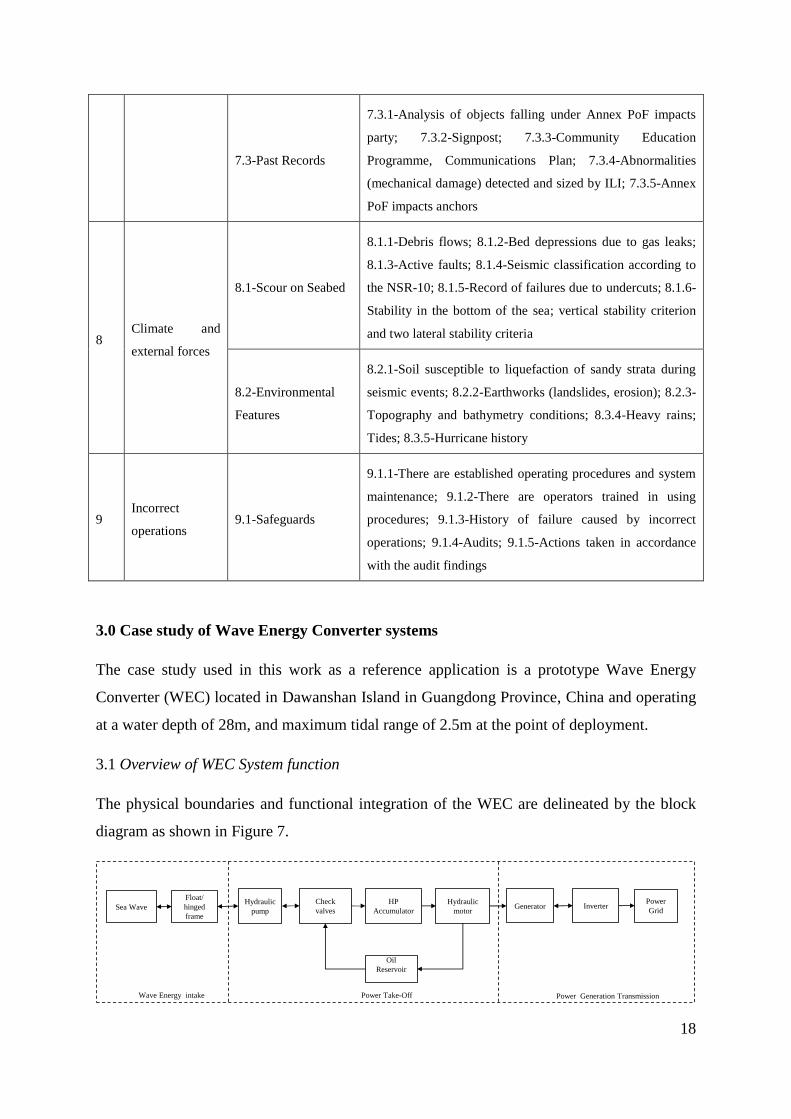
3.0 Case study of Wave Energy Converter systems

The case study used in this work as a reference application is a prototype Wave Energy

Converter (WEC) located in Dawanshan Island in Guangdong Province, China and operating

at a water depth of 28m, and maximum tidal range of 2.5m at the point of deployment.

3.1 Overview of WEC System function

The physical boundaries and functional integration of the WEC are delineated by the block

diagram as shown in Figure 7.

Sea Wave

Float/

hinged

frame

Hydraulic

pump

Hydraulic

motorGenerator Inverter

HP

Accumulator

Oil

Reservoir

Power Generation TransmissionPower Take-OffWave Energy intake

Power

Grid

Check

valves

19

Figure 7 A Simplified Block diagram of a Wave Energy Converter

WEC abstracts energy potential from the sea waves and makes it available to primary users

in the form of electric power through a series of electromechanical conversion processes.

The energy acquisition system is a hemispherical shaped buoy suspended at the tip end of a

hinged frame. When intercepted by an incident wave, the buoy heaves while the frame

observes a revolute motion about an axis (of revolution). The frame itself is held in position

by an arm fixed to the stationary ship, as shown in Figure 8. The revolution of the frame

causes a linear reciprocating motion of the double-acting rod of a hydraulic cylinder which

in turn pumps fluid to the hydraulic motor generator set, through a high pressure gas

accumulator and network of steel pipes. Low-energy hydraulic oil drains into the reservoir

where the oil are temporarily stored and have their remaining residual energy dissipated as

heat before being returned to the cylinder.

Figure 8: Wave Energy Converter

3.2 Analysis of selected subsystems of a WEC

Floating buoy: A floating buoy develops a buoyant force which induces a heave motion

[66]. Wave buoys and boats operate in a similar environment and are made of similar

material (carbon fibre reinforced composites) which should have similar failure modes.

Slamming of waves on the buoy causes overload and impacts which can cause fractures.

Poor fabrication (manufacturing defects) reduces the resistance to loads and makes the

structure susceptible to fatigue loads. Buoys can suffer cracks in the laminated skin seen

where the gel coat has fractured. The impact of waves on stiff buoys also causes fractures

and holing.

20

Figure 9: A fractured buoy (courtesy of Wave Star Energy)

Hinged frame: The hinged frame performs a revolute motion about the (upper) revolute joint

(Figure 10B) of the fixed arm extending from the ship and driving a double-acting rod of the

hydraulic cylinder bolted to lower the revolute joint. The frame is hollow and made of mild

carbon steel and operates in the splash zone. This implies that a high rate of internal and

external corrosion is likely. This however, could be aggravated by biofouling.

Figure 10 A wave energy converter: (A) general description, (B): Hinged frame

In addition, failure could possibly be initiated in the hinged frame due to welding/assembly/

construction activities and/or defects suffered during manufacturing, fatigue, overloading and

impact, and the possibility of third-party damage from fishing trawlers etc.

Hydraulic cylinder and double-acting rod: The rod observes translational reciprocating

motion about the cylinder bore. This pumps oil to the hydraulic motor. The rod is a 40 Ni-Cr

plated material, manufactured and tested based on DIN ISO 6022. Being that Ni-Cr alloy is

highly resistant to corrosion, implies that the rod is least susceptible to corrosion attack,

Revolute joint

Immovable joint

(Bolt & Nut)

Cylinder bore

Double acting rod

Rod extension

Buoy

Immovable joint

(Welded)

BA

Revolute joint

Revolute

joint

Revolute joint

Revolute joint

Hinge frame

21

however, there is the possibility of buckling under slamming waves due to overloading or

impact. Figure 11 shows a schematic of a hydraulic cylinder.

Figure 11 Longitudinal cross-section of double-rod double-acting cylinder

Other damages common to these structures, as reported in [67] are due to O-rings, cracking

of glands, damage to bearings and seals. These damages are associated with misalignment of

the load (e.g., bent rod). They cause poor clearances through which leakages can occur.

Another cause of poor clearance is bad assembly. A split weld around the base and ports of

cylinders is another damage feature commonly observed. These are caused by stress-

increasing mechanisms, such as fatigue, and/or stress-induced, such as manufacturing defect,

welding, assembly and construction. There is the possibility of fracture from being operated

beyond recommended conditions. Such mechanisms are considered here under “Incorrect

operation”. Lastly, contamination of the hydraulic fluid by seawater, and corroded, eroded or

worn out parts, such as the end cap can potentially cause failure in delivering the hydraulic

fluid to the motor. This has a root cause as wrong operations are usually from wrong filter

size or operating at a high case pressure.

Motor and Generator: The hydraulic cylinder transfers the fluid at high pressure to the motor

which turns the turbine. The major failure modes of motor and generator are highlighted in

studies by [68–70]. They include but not restricted to, excessive leakage, seal failure and

noise. At a component level the failure modes are identified as follows; corrosion (in winding

and magnets), spalling, wear (in bearing and blades), overload - impact (seal, blade, shaft and

bearing), adjustment error during welding assembly, construction and/or manufacturing

leading to misalignment of shaft, rotor asymmetry, bearing shells and/or roller element,

fatigue as experienced in shaft, slip ring and blade.

Forward StrokeBackward Stroke

Piston rod Port (A) Chamber (A) PistonPiston seal Chamber (B) Cylinder Bore Port (B)

22

Pipeline: The pipeline serves as a channel through which hydraulic fluid moves from the

cylinder to the motor-generator set. This may suffer crack or burst (in the worst cases) due to

overloading and impact. The occurrence of these failure modes could be further aggravated

by internal and/or external corrosion at a rate that is influenced by parameters such as

ambient temperature and moisture content, corrosivity of hydraulic fluid etc. Fatigue may

result from dynamics associated with fluid flowing in a pipe or from vibration due to

assembly error, i.e., too big a clearance, resulting in misalignment and mostly caused by

errors in welding, assembly and construction and/or manufacturing defects.

Gas accumulator: The gas accumulator is used to maintain stability of flow by keeping the

pressure of the pipeline at the required level. In bladder-type gas accumulators, the flexible

bladder holds the compressible gas at the pre-charged pressure and may rupture in the event

of overloading or impact during pre-charging or an out-of-proportion reduction in system

pressure. Other causes of rupture are incorrect compression ratio, incorrect pre-charge

pressure [71] which are all incorrect operations. Fatigue failure may also be experienced in

the spring and poppet assembly of the gas accumulator.

Valves: A pattern can be drawn between type of valve and failure. However, reference is

made here of generic types as found in [72–74]. Valves used in hydraulic systems, such as a

WEC to control behaviour of the hydraulic fluid, are of three types; Pressure valve, Flow

valve and Directional valve. Valve faults such as abrasion and wear usually have, as a causal

factor, improper assembly which creates uneven loading and tilting of the valve-plate. Valves

may experience other failures, such as internal corrosion, erosion, valve defects, mechanical

failure, fatigue and wear. Mechanical failure results from actions such as welding, assembly

and construction, and incorrect/defective/improper operational procedures (such as wrong

specification, human factor). It is very common to expect incorrect operation where

manufacturing and material defects are observed, where in fact, the problem is not the valve

itself but something that has been done to affect the valve operation. This is said to constitute

50% of the causes of valve incidents [72].

3.3 Demonstration of Implementation of 3-D framework

This section demonstrates the implementation of the 3-D framework, as documented in

section 2, on a real system of a WEC. A single variable – microbial activity level in the

sediment – of the threat of external corrosion (Table 2) is used for demonstrative purposes in

23

order to illustrate the concept of parameters and variables. Table 3 shows the performance of

the components of a WEC exposed to microbial activity. Score has been elicited according to

current conditions of the variables. The weights of the criteria are derived by the point

allocation method [42]. In a more detailed assessment, it is recommended that a more robust

method such a AHP [34,75–77] be used in determining the weights. The evaluation was

carried out by a team of five experts involved in the WEC project and drawn from Cranfield

University, UK and the National Ocean Technology Center, Tianjin, China. Each of the

components of the WEC had been assessed under the parameters and had scores assigned to

them as provided by the evaluation scale.

24

Table 3 Evaluation based on one variable of external corrosion

Variable Parameters

Wei

gh

t (%

)

Evaluation scale

Components list

Wav

e b

uo

y

Hinge frame Hydraulic cylinder

Pip

elin

e

Ho

se

Val

ve

Accumulator Motor and Generator

Fra

me

Rev

olu

te j

oin

t

Wel

d j

oin

t

Pis

ton

Cy

lind

er

Ro

d

Sea

l

Bea

rin

g

Bla

dd

er

Sp

ring

Po

pp

et

Bea

rin

g

Bla

de

Sh

aft

Mag

net

Win

din

g

Sea

l

Microbial

activity

level in

sediment

Class of Sediment 15 Mud 5

5 5 4 4 3 3 2 3 2 4 5 4 2 0 0 2 2 2 0 0 3

Sand-mud 3

Sand or rock 1

Not applicable 0

Organic content in

sediment (sludge)

20 If mud High 3

2 2 2 0 0 0 0 0 0 0 0 0 0 0 0 0 0 0 0 0 0

Medium 2

Low 0

If sand High 5

Medium 3

Low 2

Water depth 15 Superficial (<200 ft) 5

5 5 5 5 0 0 0 0 0 0 0 0 0 0 0 0 0 0 0 0 0 Deeper (>200 ft)) 2

Not applicable 0

Availability of

Nitrogen and

Phosphorous

20 High organic content+

N&P

5

5 5 5 5 0 0 0 0 0 0 2 2 0 0 0 0 0 0 0 0 0 Low organic content +

N&P

2

Low N&P 0

Background

Temperature

30 > 10

o C 5

2 2 2 2 5 5 5 5 5 5 2 2 5 5 5 5 5 5 5 5 5 < 10o C

2

Not applicable 0

25

The set of positive-ideal, 𝐴+and negative-ideal, 𝐴−solutions as derived for the normalized

decision matrix from (8) and (9) respectively are:

A* = {0.014, 0.051, 0.035, 0.039, 0.017} (13)

A- = {0.000, 0.003, 0.001, 0.001, 0.007} (14)

Measures of separation from positive and negative ideal solutions as derived from (10) and

(11) respectively are:

*

iS = {0.010, 0.010, 0.011, 0.050, 0.071, 0.071, 0.071, 0.071, 0.071, 0.071, 0.065, 0.065, 0.071,

0.072, 0.072, 0.071, 0.071, 0.071, 0.072, 0.072, 0.071} (15)

iS = {0.072, 0.072, 0.072, 0.052, 0.013, 0.013, 0.012, 0.013, 0.012, 0.015, 0.020, 0.019, 0.012,

0.010, 0.010, 0.012, 0.012, 0.012, 0.010, 0.010, 0.013} (16)

The similarity to both 𝑆+& 𝑆− solutions is computed as given in (12).

*

iC = {0.874, 0.874, 0.870, 0.512, 0.157, 0.157, 0.141, 0.157, 0.141, 0.175, 0.238, 0.222, 0.141,

0.126, 0.126, 0.141, 0.141, 0.141, 0.126, 0.126, 0.157}. (17)

The risk performance indices for the different components are expressed in (17). This is

presented in bar chart form in Figure 12.

Figure 12 Risk performance indices for different component from exposure to microbial induced

external corrosion

0

0.05

0.1

0.15

A B C D E F G H I J K L M N O P Q R S T U

Components

Wave buoy

Hinge frame

Frame Rev. Joint

Frame Weld. Joint

Cylinder piston

Cylinder

Cylinder rod

Cylinder seal

Cylinder bearing

Pipelines

Hoses

Valves

Acc. bladder

Acc. Spring

Acc. Poppet

Motor bearing

Generator blades

Motor shaft

Generator magnets

Generator windings

Generator seals

A:

B:

C:

D:

E:

F:

G:

H:

I:

J:

K:

L:

M:

N:

O:

P:

Q:

R:

S:

T:

U:

Relative risk

19% 81%

High-risk Low-risk

26

It can be deduced from Figure 12 that 54% of the risk of external corrosion due to activities

of microbial activities lies in just 19% of the components. These components are: wave buoy

and the frame, and the two joints. The results of a full scale implementation of the framework

on the structure and incorporating variables from all the threats and failure modes will be

presented in the next section.

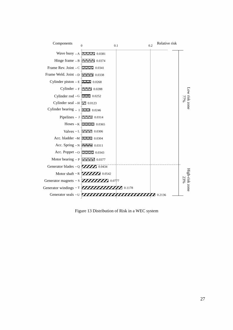
4.0 Result and Discussion

A total of 21 components of the WEC were analysed and evaluated against 112 parameters of

the nine generic failure mechanisms. Figure 13 shows the results of the global aggregation

approach i.e., the plot of [𝑷𝑽]𝑚 as described in 2.3.3. It can be seen from Figure 13 that

about half of the system’s risk is concentrated in just 23% of the components: Generator

components –seals, generator’s windings and magnet, motor shaft, and generator blade. The

implication of this from an IRM perspective is that it would be inefficient to inspect, repair

and maintain all components with the same level of priority. Rather, a recommended IRM

plan should identify the 23% of components and raise their priority level.

The result obtained from full implementation of local aggregation approach; the matrix

[ ]𝑚 𝑛

(see section 2.3.3) is presented in Table 4. The plotted of these values are as

shown in the scatter of Figure 15. It shows the relative activity levels of various failure

modes/mechanisms in each component. As can be seen from Figure 15, errors from welding-

assembly-construction (WAC) constitutes the active threats to components wave buoys,

hinge frame, revolute joints(frame), frame welds, and cylinder piston. From IRM point of

view, these threats should be inspected in those components. Similarly, the first three active

failure modes/ mechanisms for pipeline (component J) are MAD, INC, and error of WAC.

The threats that develop through these failure modes/mechanisms should be monitored

through inspection. Another way the data of Table 4 can be treated is to perform row –sum

which gives the total risk content of the components. This gives an interesting pattern when

normalised (Figure 14) that captures the distributions of failure mode/mechanism –specific

risks for each component of the system. This analysis avails the assets manager/engineer the

knowledge of susceptibility of the various components of the asset to the failure

mode/mechanisms; the results which will serves as a supports tool to the asset

manager/engineer who may be required to defend maintenance decisions from time to time

such as setting priority of failure mode to mitigate for each component.

27

Figure 13 Distribution of Risk in a WEC system

0.0381

0.0374

0.0341

0.0338

0.0268

0.0288

0.0252

0.0123

0.0246

0.0314

0.0365

0.0306

0.0304

0.0311

0.0343

0.0377

0.0434

0.0542

0.0777

0.1178

0.2136

0 0.1 0.2

A

B

C

D

E

F

G

H

I

J

K

L

M

N

O

P

Q

R

S

T

U

Components Relative riskH

igh-risk

zon

e

23

%

Lo

w risk

zon

e

77

%

Wave buoy

Hinge frame

Frame Rev. Joint

Frame Weld. Joint

Cylinder piston

Cylinder

Cylinder rod

Cylinder seal

Cylinder bearing

Pipelines

Hoses

Valves

Acc. bladder

Acc. Spring

Acc. Poppet

Motor bearing

Generator blades

Motor shaft

Generator magnets

Generator windings

Generator seals

28

Table 4 Performance of the components under Failure modes

Component Risk sources and Events

INC ETC WAC MAD FTG O&I TPD ICO CEF

Wave buoy 0.3717 0.6109 0.9857 0.1024 0.7154 0.3365 0.6470 0.4967 0.8651

Hinge frame 0.3802 0.6117 0.9942 0.4503 0.5449 0.4364 0.6454 0.4967 0.3737

Frame Rev. Joint 0.2930 0.6109 0.9848 0.1646 0.3885 0.2123 0.6454 0.4965 0.4305

Frame Weld Joints 0.2927 0.6109 0.9866 0.2178 0.7099 0.3899 0.6454 0.4949 0.3737

Cylinder piston 0.0819 0.2603 0.9995 0.1634 0.3764 0.1401 0.3127 0.1702 0.4531

Cylinder 0.1963 0.1152 0.0682 0.0890 0.3680 0.4757 0.5827 0.1702 0.4080

Cylinder rod 0.1650 0.1246 0.5677 0.1537 0.4580 0.3281 0.5828 0.1702 0.3087

Cylinder seal 0.1465 0.1204 0.5111 0.0859 0.3756 0.4103 0.3222 0.1702 0.1910

Cylinder bearing 0.0746 0.1465 0.5120 0.0890 0.1975 0.4380 0.3897 0.1702 0.1349

Pipeline 0.7573 0.1263 0.7436 0.7797 0.5286 0.4399 0.3582 0.1702 0.3087

Hoses 0.7881 0.2061 0.5482 0.5799 0.7658 0.5276 0.5702 0.5572 0.3737

Valve 0.6955 0.2199 0.5500 0.3197 0.4644 0.1679 0.0786 0.1605 0.3087

Accumulator Bladder 0.0637 0.0168 0.5110 0.2170 0.4580 0.5878 0.0103 0.1605 0.0713

Accumulator Spring 0.0652 0.1022 0.2587 0.3197 0.5815 0.2470 0.0103 0.1605 0.1349

Poppet 0.0652 0.1004 0.5142 0.3230 0.5936 0.3863 0.0103 0.1605 0.0000

Motor Bearing 0.0750 0.4204 0.5122 0.1577 0.2846 0.4413 0.1015 0.5082 0.0713

Generator blades 0.0736 0.4202 0.5539 0.1635 0.0668 0.1562 0.0103 0.5082 0.0000

Motor shaft 0.1424 0.4202 0.6334 0.5803 0.5594 0.7289 0.0103 0.5035 0.1349

Generator magnet 0.0512 0.0164 0.5099 0.0265 0.3885 0.2041 0.0103 0.1605 0.0713

Gen. Windings 0.1359 0.0913 0.5099 0.3207 0.1538 0.2876 0.0103 0.1605 0.0000

Motor seals 0.0759 0.1011 0.5101 0.0276 0.5815 0.4297 0.1015 0.1605 0.0713

INC = Internal corrosion; ETC = External corrosion; WAC = Welding, Assembly, and Construction; MAD =

Manufacturing defect; FTG = Fatigue; O&I = Overloading & Impact; TPD = Third party damage; ICO =

Incorrect operation; CEF = Climate & External forces

29

Figure 14 Normalized sum of component’s failure mode-specific risk score

Figure 15: Contribution of failure modes towards components risk

0% 10% 20% 30% 40% 50% 60% 70% 80% 90% 100%

Wave buoy

Hinge frame

Frame Rev. Joint

Frame Weld Joints

Cylinder piston

Cylinder

Cylinder rod

Cylinder seal

Cylinder bearing

Pipeline

Hoses

Valve

Accumulator Bladder

Accumulator Spring

Poppet

Motor Bearing

Generator blades

Motor shaft

Generator magnet

Gen. Windings

Motor seals

Percentage contribution to component risk of failure

Internal corrosion External corrosion Welding, Assembling & Construction

Manufacturing defect Fatigue Overloading & Impact

Third party damage Incorrect operation Climate & External forces

To

tal risk co

nten

t of th

e com

po

nen

ts2.0592

1.6700

1.4389

3.7133

1.9528

2.5722

2.1534

1.8800

2.0965

2.9651

4.9167

4.2125

2.1525

2.3332

2.8588

2.4733

2.9576

4.7218

4.2264

4.9335

5.1314

A B C D E F G H I J K L M N O P Q R S T U

A: Wave buoy B: Hinge frame C: Frame Rev. Joint D: Frame Weld. Joint E: Cylinder piston F: Cylinder G: Cylinder rod

H: Cylinder seal I: Cylinder bearing J: Pipelines K: Hoses L: Valves M: Acc. Bladder N: Acc. Spring O: Acc. Poppet

P: Motor bearing Q: Generator blades R: Motor shaft S: Generator magnets T: Generator windings U: Generator seals

0.0

0.2

0.4

0.6

0.8

1.0

1.2

INC

EXT

WAC

MAD

FTG

O&I

TPD

IOP

CEF

30

5 Conclusions

In this paper, a framework is developed to support prioritisation of components of offshore

engineering systems based on risk levels for intervention action, leading to inspection, repair

and maintenance. The advantage of this framework is the systematic way it incorporates a

wide range of evaluation criteria and still demonstrates clarity in risk level estimation,

aggregation and prioritisation in a manner that ensures repeatability. Precision of ranking is

enhanced through a combination of actions; firstly, an updatable database is developed for

failure modes, risk variables and parameters. These parameters hold information on operating

conditions –normal and/or upset, current and projected future of the components, required in

order to make informed judgement of occurrence, severity of failure modes and safeguards.

This enhances the traceability of the assessment outcomes to the source data. The direct

implication of this is that the model can easily be updated with the latest information as

obtained from inspection findings. Also, it addresses epistemic uncertainties and ensures

uniformity of application during the evaluation process. Secondly, it minimizes subjectivity

in risk evaluation through consideration of weighting at parameters levels – which qualify the

variables of failure modes. This is in contrast to the practice in FMEA where weights are

considered at the failure mode level resulting in a high subjective model. For demonstrative

purposes, these weights had been derived through a point allocation process. Thirdly, it

provides a systematic way of application of risk assessment across components of complex

engineering systems such that is possible to perform risk assessment of different components

simultaneously with a lower risk of subjectivity, and reduced inaccuracy.

The framework has been implemented on a real offshore structure, a WEC, and the results

obtained showed to have practical implications to efficient IRM management of components

of offshore energy structures. Initial prioritisation of components by global aggregation

approach is usually based on previous inspection records. Subsequent prioritisation requires

up-to-date information via inspections finding that target prioritised components. If a

component shows no sign of developing defect – by maintaining the same relative position in

the priority scale for recurring inspection – it should be credited by increasing the time to the

following inspection. In other words, the question of “how often to inspect” is addressed.

More so, the efficiency of IRM can be further enhanced by suggesting “what to inspect”. This

is where the second analysis –local aggregation approach –finds application. A scatter plot

31

of [ ]𝑚×𝑛

(Figure 15) shows the failure modes/mechanisms arranged in order of

decreasing activity level. This result is vital for defence of decisions on budget allocations for

inspection repair and maintenance.

For the case study presented, it should be noted that the result is validated based on the

experience of the participating researchers in the project. This is due to the fact that the area

of renewable energy is relatively new, as such there are not enough data for validation.

Though an attempt is made in this paper to list as many failure mode/mechanism and

variables and parameters as possible, such analysis inherently is perforce finite; whereas in

reality such list is infinite. However, the model is highly flexible in terms of accommodating

new found failure modes/mechanisms, variables and parameters and can be adapted for many

purposes. Identification and inclusion of new failure modes/mechanisms, variables and

parameters as more knowledge is gained is dependent on the experience assessor.

Acknowledgements: This work was supported by grant EP/M020339/1 for Cranfield

University, from the UK Engineering and Physical Sciences Research Council (EPSRC).

6.0 References

[1] Linares P. Multiple Criteria Decision Making and Risk Analysis as Risk Management

Tools for Power Systems Planning. IEEE Trans Power Syst 2002;17:895–900.

[2] Sakai S. Risk-based Maintenance. East Japan Railw Co 2010:29–44.

[3] Aven T, Vinnem JE, Wiencke HS. A decision framework for risk management, with

application to the offshore oil and gas industry. Reliab Eng Syst Saf 2007;92:433–48.

doi:http://dx.doi.org/10.1016/j.ress.2005.12.009.

[4] ISO. Risk management – Code of practice and guidance for the implementation of BS

ISO 31000. 2011.

[5] Linkov I, Satterstrom FK, Kiker G, Batchelor C, Bridges T, Ferguson E. From

comparative risk assessment to multi-criteria decision analysis and adaptive

management: Recent developments and applications. Environ Risk Manag - State Art

32

2006;32:1072–93. doi:http://dx.doi.org/10.1016/j.envint.2006.06.013.

[6] Pluessa DN, Grosob A, Meyer T. Expert Judgements in Risk Analysis: a Strategy to

Overcome Uncertainties. Chem Eng 2013;31.

[7] Bea RG. Risk Assessment and Management : Challenges of the Macondo Well

Blowout Disaster. 2011.

[8] Geary W. R isk Based Inspection: a Case Study Evaluation of Offshore Process Plant.

vol. HSL/2002/2. Sheffield: Health and Safety Laboratory; 2002.

[9] Chan HK, Chan FT. A comprehensive survey and future trend of simulation study on

FMS scheduling. J Intell Manuf 2004;15:87–102.

[10] Heller S. Managing industrial risk—Having a tested and proven system to prevent and

assess risk. Pap Present 2004 Annu Symp Mary Kay O’Connor Process Saf Cent Pap

Present 2004 Annu Symp Mary Kay O'Connor Process Saf Cent 2006;130:58–63.

doi:http://dx.doi.org/10.1016/j.jhazmat.2005.07.067.

[11] Garvey PR. Analytical methods for risk management.pdf. Bedford, Massachusetts,

USA: CRC Press; 2009.

[12] BS EN 60812. Analysis techniques for system reliabilityProcedure for failure mode

and effects analysis (FMEA). London: British Standards Institute; 2006.

[13] Mikulak R, McDermott R, Beauregard M. The basics of FMEA. 2nd ed. New York,

NY 10016: Taylor & Francis; 2011.

[14] Moore, W, H,, and Bea, R G. Management of Human Error in Operations of Marine

Systems, Report No, HOE-93-1, Final Joint Industry Project Report. California,

Berkeley: 1993.

[15] Bea RG. Quantitative and Qualitative Risk Analyses - The Safety of Offshore

Platforms. Offshore Technol Conf 1996. doi:10.4043/8037-MS.

[16] Stamatis, D.H. Failure Mode and Effect Analysis: FMEA from Theory to Execution.

2003. doi:10.2307/1268911.

[17] Lipol LS, Hag J. Risk analysis method:FMEA/FMECA in the organizations. Int J

33

Basic Appl Sci 2011;11:74–82.

[18] Carlson C. Effective FMEAs: Acheiving safe, reliable economical products and

processes using failure mode effect and analysis. Hoboken, NewJersey, USA: Wiley

and sons inc.; 2012.

[19] Wang Y, Cheng G, Hu H, Wu W. Development of a risk-based maintenance strategy

using FMEA for a continuous catalytic reforming plant. J Loss Prev Process Ind

2012;25:958–65.

[20] Marlow DR, Beale DJ, Mashford JS. Risk-based prioritization and its application to

inspection of valves in the water sector. Reliab Eng Syst Saf 2012;100:67–74.

doi:http://dx.doi.org/10.1016/j.ress.2011.12.014.

[21] Hodges S, Spicer K, Barson R, John G, Oliver K, Tipton E. High level corrosion risk

assessment methodology for oil & gas systems. NACE Int. Corros. 2010. Conf. Expo,

San Antonio, TX, USA.: NACE International; 2010, p. 1–15.

[22] Bowles JB. An assessment of RPN Prioritization in a Failure Modes Effect and

Criticality Analysis. Annu. Reliab. Maintainab. Symp., Tampa, FL. USA: IEEE; 2003,

p. 380.

[23] Kaplan S, Garrick BJ. On the quantitative definition of risk. Risk Anal 1981;1:11–27.

[24] Hobbs BF. A Comparison of Weighting Methods in Power Plant Siting. Decis Sci

1980;11:725–37. doi:10.1111/j.1540-5915.1980.tb01173.x.

[25] Hobbs BF. What can we learn from experiments in multiobjective decision analysis?

IEEE Trans Syst Man Cybern 1986;16:384–94.

[26] Weber M, Borcherding K. Behavioral influences on weight judgments in multiattribute

decision making. Eur J Oper Res 1993;67:1–12. doi:10.1016/0377-2217(93)90318-H.

[27] Pugsley AG. Report on Structural Safety. London, UK: 1955.

[28] Franceschini F, Galetto M. A new approach for evaluation of risk priorities of failure

modes in FMEA. Int J Prod Res 2001;39:2991–3002.

[29] Linkov I, Seager TP. Coupling multi-criteria decision analysis, life-cycle assessment,

34

and risk assessment for emerging threats. Environ Sci Technol 2011;45:5068–74.

doi:10.1021/es100959q.

[30] Reaves CC. Quantitative research for the behavioral sciences. New York, USA: John

Wiley; 1992.

[31] Hwang CL, Yoon K. Multiple attribute decision making. 1981. Lect Notes Econ Math

Syst 1981.

[32] Zeleny M. Multiple criteria decision making. New York, USA: McGraw-Hill; 1982.

[33] Sachdeva A, Kumar D, Kumar P. Multi-factor failure mode critical analysis using

TOPSIS. J Ind Eng 2009;5:1–9.

[34] Kutlu AC, Ekmekçioǧlu M. Fuzzy failure modes and effects analysis by using fuzzy

TOPSIS-based fuzzy AHP. Expert Syst Appl 2012;39:61–7.

doi:10.1016/j.eswa.2011.06.044.

[35] Kolios A, Collu M, Chahardehi A, Brennan FP, Patel MH. A multi-criteria decision

making method to compare support structures for offshore wind turbines. EWEC

Warsaw 2010.

[36] Lozano-Minguez E, Kolios AJ, Brennan FP. Multi-criteria assessment of offshore

wind turbine support structures. Renew Energy 2011;36:2831–7.

doi:http://dx.doi.org/10.1016/j.renene.2011.04.020.

[37] Kolios AJ, Rodriguez-Tsouroukdissian A, Salonitis K. Multi-criteria decision analysis

of offshore wind turbines support structures under stochastic inputs. Ships Offshore

Struct 2014:1–12.

[38] Martin H, Spano G, Küster JF, Collu M, Kolios AJ, Spano G, et al. Application and

extension of the TOPSIS method for the assessment of floating offshore wind turbine

support structures 2012. doi:10.1080/17445302.2012.718957.

[39] Kolios A, Read G, Ioannou A. Application of Multi-Criteria Decision Making to Risk

Prioritization in Tidal Enrgy Developments. Int J Sustain Energy 2013;http://www:1–

17.

[40] Zavadskas EK, Turskis Z, Tamošaitiene J. Risk assessment of construction projects. J

35

Civ Eng Manag 2010;16:33–46. doi:10.3846/jcem.2010.03.

[41] Tamosaitience J, Zavadskas EK, Turskis Z. Multi-criteria risk assessment of a

construction project. Procedia Comput Sci 2013;17:129–33.

doi:10.1016/j.procs.2013.05.018.

[42] Zardari NH, Ahmed K, Shirazi SM, Yusop Z Bin. Weighting Methods and Their

Effect on Multi Criteria Decision Making Model Outcomes in Water Resources

Management. Malaysia: Springer; 2015.

[43] Wang JJ, Jing YY, Zhang CF, Zhao JH. Review on multi-criteria decision analysis aid

in sustainable energy decision-making. Renew Sustain Energy Rev 2009;13:2263–78.

doi:10.1016/j.rser.2009.06.021.

[44] Nijkamp P, Rietveld P, Voogd H. Multicriteria Evaluation in Physical Planning.

Groningen: Elsevier Science Publishers; 1990.

[45] Malczewski J. GIS and Multicriteria Decision Analysis. John Wiley & Sons, Inc.,;

1999.

[46] Mardle SJ. Energy Decisions and the Environment: A Guide to the Use of Multicriteria

Methods. vol. 53. 2002. doi:DOI 10.1057/palgrave.jors.2601379.

[47] Maheswaran K, Loganathan T. A novel approach for prioritisation of failure modes in

FMEA using MCDM. Int J Eng Res Appl 2013;3:733–9.

[48] Figueiredo MS, Oliveira MD. Prioritizing Risks Based on Multicriteria Decision Aid

Methodology: Development of Methods Applied to ALSTOM Power. Ind. Eng. Eng.

Manag., Hong Kong: IEEE; 2009, p. 1568–72.

[49] Bevilacqua M, Braglia M. The analytical hierarchy process applied to maintenance

strategy selection. Reliab Eng Syst Saf 2000;70:71–83.

[50] Moan T. The Alexander L. Kielland accident-30 year Later. Proc 1st Wallace Lect

Rept MITSC 81-8, Sea Grant Coll Program, Dept Ocean Eng MIT Cited Moan,

Torgier Int J Offshore Polar Eng 1981;17:1–21.

[51] Paé-Cornell ME. Learning from the Piper Alpha accident: A postmortem analysis of

technical and organizational factors. Insur Math Econ 1993;13:165. doi:10.1016/0167-

36

6687(93)90921-B.

[52] Bea GR. Accident on 25 July 2000 at La Patte d’Oie in Gonesse (95) to the Concorde

registered F-BTSC operated by Air France (English translation). vol. f-sc000725.

France: Ministry of Equipment, Transportation and Housing-Bureau of Investigation

and Analysis for the Safety of Civil Aviation; 2002.

[53] Nivolianitou Z, Konstandinidou M, Michalis C. Statistical analysis of major accidents

in petrochemical industry notified to the major accident reporting system (MARS). J

Hazard Mater 2006;137:1–7. doi:http://dx.doi.org/10.1016/j.jhazmat.2004.12.042.

[54] NASA Safety Center. The Case for Safety: The Case for Safety. Syst Fail Case Stud

2013;7:11–44.

[55] Graham B, Reilly WK, Beinecke F, Boesch DF, Garcia TD, Murray CA. Deep Water:

The Gulf Oil Disaster and the Future of Offshore Drilling. 2011.

doi:10.3723/ut.30.113.

[56] WOAD. Worldwide Offshore Accident Databank 2016.

[57] International Association of Oil and Gas Producers. Risk Assessment Data Directory:

Major accidents. 2010.

[58] HSE Oil & Gas UK. Accident Statistics for Offshore Units on the UKCS 1990-2007.

vol. part 1. 2009.

[59] Oil and Gas UK. Health & Safety Report 2014. 2014.

[60] Ian S, Ukcs W, Recovery M, Report F. Report by Sir Ian Wood UKCS Maximising

Recovery Review: Final Report 2014:1–18.

[61] SINTEF. OREDA-Offshore Reliability Data Handbook. 4th ed. OREDA Participants;

2002.

[62] Catapult & Crown Estate. SPARTA: System Performance, Availability and Reliability

Trend Analysis n.d. https://www.sparta-offshore.com/spartaweb/login (accessed 1

January 2016).

[63] API 581. Risk-Based Inspection Technology 2008.

37

[64] CEN. Risk-Based Inspection and Maintenance Procedures for European Industries

(RIMAP). vol. CWA 15740: Rue de Stassart,Brussels: European Committee for

Standardisation; 2008.

[65] API. RP 571, Damage Mechanisms Affecting fixed Equipment in the Refining

Industry. 2003.

[66] SI Ocean. Ocean Energy: State of the Art. EU Proj Rep 2012:79. http://si-

ocean.eu/en/upload/docs/WP3/Technology Status Report_FV.pdf. (accessed 18

October 2015).

[67] Wallis KW. The Top 10 Reasons for Hydraulic Cylinder Failures - And What To Do

About Them 2010. http://ezinearticles.com/?The-Top-10-Reasons-for-Hydraulic-

Cylinder-Failures---And-What-To-Do-About-Them&id=5474641 (accessed 19

October 2015).

[68] Tchakoua P, Wamkeue R, Ouhrouche M, Slaoui-Hasnaoui F, Tameghe TA, Ekemb G.

Wind Turbine Condition Monitoring: State-of-the-Art Review, New Trends, and

Future Challenges. Energies 2014;7:2595–630.

[69] Grimwade J, Hails D, Robles E, Salcedo F, Bard J, Kracht P, et al. Review of Relevant

PTO Systems. D2.03. 2012.

[70] BS 5760-5. Reliability of systems, equipment and components. Part 5. Guid to Fail

Modes, Eff Crit Anal (FMEA FMECA) 1991.

[71] Casey B. How to Avoid Hydraulic Accumulator Failure. Hydraul Supermarket.com

2014. http://www.hydraulicsupermarket.com/blog/all/how-to-avoid-hydraulic-

accumulator-failure/.

[72] Peters J. Assessment of valve failures in the offshore oil & gas sector. 2003.

[73] Geary W. Failure analysis of solenoid valve components from a hydraulic roof

support. Case Stud Eng Fail Anal 2013;1:209–16. doi:10.1016/j.csefa.2013.07.004.

[74] Casey B. How to Solve and Prevent Hydraulic Problems. Hydraul Com 2005.

http://www.hydraulicsupermarket.com/books (accessed 29 October 2015).

[75] Seçme NY, Bayrakdaroğlu A, Kahraman C. Fuzzy performance evaluation in Turkish

38

Banking Sector using Analytic Hierarchy Process and TOPSIS. Expert Syst Appl

2009;36:11699–709. doi:http://dx.doi.org/10.1016/j.eswa.2009.03.013.

[76] DAgkinis I, Theodoros L, Nikitakos N. Operational failure prevention methodology

for offshore systems using multiple criteria decision-making process. J Polish Saf

Reliab Assoc 2012;3:15–22.

[77] Perera N, Sutrisna M. The Use of Analytic Hierarchy Process (AHP) in the Analysis of

Delay Claims in Construction Projects in the UAE. Built Hum Environ Rev

2010;3:29–48.