multi degrees of freedom systems - mdof · multidof systems giacomoboffi introductory remarks the...
TRANSCRIPT

Multi DoFSystems
Giacomo Boffi
IntroductoryRemarks
TheHomogeneousProblem
Modal Analysis
Examples
Multi Degrees of Freedom SystemsMDOF
Giacomo Boffi
http://intranet.dica.polimi.it/people/boffi-giacomo
Dipartimento di Ingegneria Civile Ambientale e TerritorialePolitecnico di Milano
March 20, 2018

Multi DoFSystems
Giacomo Boffi
IntroductoryRemarks
TheHomogeneousProblem
Modal Analysis
Examples
Outline
Introductory RemarksAn ExampleThe Equation of Motion, a System of Linear Differential EquationsMatrices are Linear OperatorsProperties of Structural MatricesAn example
The Homogeneous ProblemThe Homogeneous Equation of MotionEigenvalues and EigenvectorsEigenvectors are Orthogonal
Modal AnalysisEigenvectors are a baseEoM in Modal CoordinatesInitial Conditions
Examples2 DOF System

Multi DoFSystems
Giacomo Boffi
IntroductoryRemarksAn Example
The Equation ofMotion
Matrices are LinearOperators
Properties ofStructural Matrices
An example
TheHomogeneousProblem
Modal Analysis
Examples
Introductory Remarks
Consider an undamped system with two masses and two degrees offreedom.
k1 k2 k3m1 m2
x1 x2
p1(t) p2(t)

Multi DoFSystems
Giacomo Boffi
IntroductoryRemarksAn Example
The Equation ofMotion
Matrices are LinearOperators
Properties ofStructural Matrices
An example
TheHomogeneousProblem
Modal Analysis
Examples
Introductory Remarks
We can separate the two masses, single out the spring forces and,using the D’Alembert Principle, the inertial forces and, finally. writean equation of dynamic equilibrium for each mass.
p2
m2x2k3x2k2(x2 − x1)
m2x2 − k2x1 + (k2 + k3)x2 = p2(t)
m1x1k2(x1 − x2)k1x1
p1
m1x1 + (k1 + k2)x1 − k2x2 = p1(t)

Multi DoFSystems
Giacomo Boffi
IntroductoryRemarksAn Example
The Equation ofMotion
Matrices are LinearOperators
Properties ofStructural Matrices
An example
TheHomogeneousProblem
Modal Analysis
Examples
The equation of motion of a 2DOF system
With some little rearrangement we have a system of two lineardifferential equations in two variables, x1(t) and x2(t):{
m1x1 + (k1 + k2)x1 − k2x2 = p1(t),
m2x2 − k2x1 + (k2 + k3)x2 = p2(t).

Multi DoFSystems
Giacomo Boffi
IntroductoryRemarksAn Example
The Equation ofMotion
Matrices are LinearOperators
Properties ofStructural Matrices
An example
TheHomogeneousProblem
Modal Analysis
Examples
The equation of motion of a 2DOF system
Introducing the loading vector p, the vector of inertial forces fI andthe vector of elastic forces fS ,
p =
{p1(t)p2(t)
}, fI =
{fI,1fI,2
}, fS =
{fS,1fS,2
}we can write a vectorial equation of equilibrium:
fI + fS = p(t).

Multi DoFSystems
Giacomo Boffi
IntroductoryRemarksAn Example
The Equation ofMotion
Matrices are LinearOperators
Properties ofStructural Matrices
An example
TheHomogeneousProblem
Modal Analysis
Examples
fS =Kx
It is possible to write the linear relationship between fS and thevector of displacements x =
{x1x2
}T in terms of a matrix product,introducing the so called stiffness matrix K.
In our example it is
fS =
[k1 + k2 −k2−k2 k2 + k3
]x = Kx
The stiffness matrix K has a number of rows equal to the number ofelastic forces, i.e., one force for each DOF and a number of columnsequal to the number of the DOF.The stiffness matrix K is hence a square matrix K
ndof×ndof

Multi DoFSystems
Giacomo Boffi
IntroductoryRemarksAn Example
The Equation ofMotion
Matrices are LinearOperators
Properties ofStructural Matrices
An example
TheHomogeneousProblem
Modal Analysis
Examples
fS =Kx
It is possible to write the linear relationship between fS and thevector of displacements x =
{x1x2
}T in terms of a matrix product,introducing the so called stiffness matrix K.In our example it is
fS =
[k1 + k2 −k2−k2 k2 + k3
]x = Kx
The stiffness matrix K has a number of rows equal to the number ofelastic forces, i.e., one force for each DOF and a number of columnsequal to the number of the DOF.The stiffness matrix K is hence a square matrix K
ndof×ndof

Multi DoFSystems
Giacomo Boffi
IntroductoryRemarksAn Example
The Equation ofMotion
Matrices are LinearOperators
Properties ofStructural Matrices
An example
TheHomogeneousProblem
Modal Analysis
Examples
fI =M x
Analogously, introducing the mass matrix M that, for our example,is
M =
[m1 00 m2
]we can write
fI = M x.
Also the mass matrix M is a square matrix, with number of rowsand columns equal to the number of DOF’s.

Multi DoFSystems
Giacomo Boffi
IntroductoryRemarksAn Example
The Equation ofMotion
Matrices are LinearOperators
Properties ofStructural Matrices
An example
TheHomogeneousProblem
Modal Analysis
Examples
Matrix Equation
Finally it is possible to write the equation of motion in matrix format:
M x+Kx = p(t).
Of course it is possible to take into consideration also the dampingforces, taking into account the velocity vector x and introducinga damping matrix C too, so that we can eventually write
M x+C x+Kx = p(t).
But today we are focused on undamped systems...

Multi DoFSystems
Giacomo Boffi
IntroductoryRemarksAn Example
The Equation ofMotion
Matrices are LinearOperators
Properties ofStructural Matrices
An example
TheHomogeneousProblem
Modal Analysis
Examples
Properties of K
I K is symmetrical.The elastic force exerted on mass i due to an unit displacementof mass j, fS,i = kij is equal to the force kji exerted on mass jdue to an unit diplacement of mass i, in virtue of Betti’stheorem (also known as Maxwell-Betti reciprocal work theorem).
I K is a positive definite matrix.The strain energy V for a discrete system is
V =1
2xTfS ,
and expressing fS in terms of K and x we have
V =1
2xTKx,
and because the strain energy is positive for x 6= 0 it followsthat K is definite positive.

Multi DoFSystems
Giacomo Boffi
IntroductoryRemarksAn Example
The Equation ofMotion
Matrices are LinearOperators
Properties ofStructural Matrices
An example
TheHomogeneousProblem
Modal Analysis
Examples
Properties of M
Restricting our discussion to systems whose degrees of freedom arethe displacements of a set of discrete masses, we have that the massmatrix is a diagonal matrix, with all its diagonal elements greaterthan zero. Such a matrix is symmetrical and definite positive.Both the mass and the stiffness matrix are symmetrical and definitepositive.
Note that the kinetic energy for a discrete system can bewritten
T =1
2xTM x.

Multi DoFSystems
Giacomo Boffi
IntroductoryRemarksAn Example
The Equation ofMotion
Matrices are LinearOperators
Properties ofStructural Matrices
An example
TheHomogeneousProblem
Modal Analysis
Examples
Generalisation of previous results
The findings in the previous two slides can be generalised to thestructural matrices of generic structural systems, with two mainexceptions.
1. For a general structural system, in which not all DOFs arerelated to a mass, M could be semi-definite positive, that is forsome particular displacement vector the kinetic energy is zero.
2. For a general structural system subjected to axial loads, due tothe presence of geometrical stiffness it is possible that for someparticular displacement vector the strain energy is zero and Kis semi-definite positive.

Multi DoFSystems
Giacomo Boffi
IntroductoryRemarksAn Example
The Equation ofMotion
Matrices are LinearOperators
Properties ofStructural Matrices
An example
TheHomogeneousProblem
Modal Analysis
Examples
The problem
Graphical statement of the problem
k1 = 2k, k2 = k; m1 = 2m, m2 = m;
p(t) = p0 sinωt.
k1
x1 x2
m2
k2
m1
p(t)
The equations of motion
m1x1 + k1x1 + k2 (x1 − x2) = p0 sinωt,
m2x2 + k2 (x2 − x1) = 0.
... but we prefer the matrix notation ...

Multi DoFSystems
Giacomo Boffi
IntroductoryRemarksAn Example
The Equation ofMotion
Matrices are LinearOperators
Properties ofStructural Matrices
An example
TheHomogeneousProblem
Modal Analysis
Examples
The steady state solution
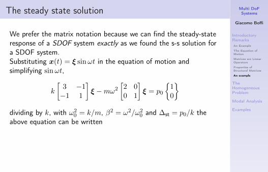
We prefer the matrix notation because we can find the steady-stateresponse of a SDOF system exactly as we found the s-s solution fora SDOF system.Substituting x(t) = ξ sinωt in the equation of motion andsimplifying sinωt,
k
[3 −1−1 1
]ξ −mω2
[2 00 1
]ξ = p0
{10
}
dividing by k, with ω20 = k/m, β2 = ω2/ω2
0 and ∆st = p0/k theabove equation can be written([
3 −1−1 1
]− β2
[2 00 1
])ξ =
[3− 2β2 −1−1 1− β2
]ξ = ∆st
{10
}.
Multi DoFSystems
Giacomo Boffi
IntroductoryRemarksAn Example
The Equation ofMotion
Matrices are LinearOperators
Properties ofStructural Matrices
An example
TheHomogeneousProblem
Modal Analysis
Examples
The steady state solution
We prefer the matrix notation because we can find the steady-stateresponse of a SDOF system exactly as we found the s-s solution fora SDOF system.Substituting x(t) = ξ sinωt in the equation of motion andsimplifying sinωt,
k
[3 −1−1 1
]ξ −mω2
[2 00 1
]ξ = p0
{10
}dividing by k, with ω2
0 = k/m, β2 = ω2/ω20 and ∆st = p0/k the
above equation can be written
([3 −1−1 1
]− β2
[2 00 1
])ξ =
[3− 2β2 −1−1 1− β2
]ξ = ∆st
{10
}.

Multi DoFSystems
Giacomo Boffi
IntroductoryRemarksAn Example
The Equation ofMotion
Matrices are LinearOperators
Properties ofStructural Matrices
An example
TheHomogeneousProblem
Modal Analysis
Examples
The steady state solution
We prefer the matrix notation because we can find the steady-stateresponse of a SDOF system exactly as we found the s-s solution fora SDOF system.Substituting x(t) = ξ sinωt in the equation of motion andsimplifying sinωt,
k
[3 −1−1 1
]ξ −mω2
[2 00 1
]ξ = p0
{10
}dividing by k, with ω2
0 = k/m, β2 = ω2/ω20 and ∆st = p0/k the
above equation can be written([3 −1−1 1
]− β2
[2 00 1
])ξ =
[3− 2β2 −1−1 1− β2
]ξ = ∆st
{10
}.
Multi DoFSystems
Giacomo Boffi
IntroductoryRemarksAn Example
The Equation ofMotion
Matrices are LinearOperators
Properties ofStructural Matrices
An example
TheHomogeneousProblem
Modal Analysis
Examples
The steady state solution
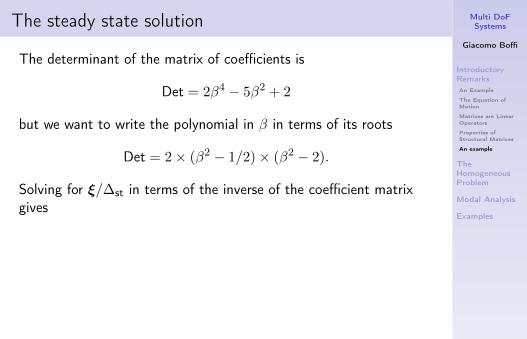
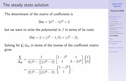
The determinant of the matrix of coefficients is
Det = 2β4 − 5β2 + 2
but we want to write the polynomial in β in terms of its roots
Det = 2× (β2 − 1/2)× (β2 − 2).
Solving for ξ/∆st in terms of the inverse of the coefficient matrixgives
ξ
∆st=
1
2(β2 − 12)(β2 − 2)
[1− β2 1
1 3− 2β2
]{10
}=
1
2(β2 − 12)(β2 − 2)
{1− β2
1
}.
Multi DoFSystems
Giacomo Boffi
IntroductoryRemarksAn Example
The Equation ofMotion
Matrices are LinearOperators
Properties ofStructural Matrices
An example
TheHomogeneousProblem
Modal Analysis
Examples
The steady state solution
The determinant of the matrix of coefficients is
Det = 2β4 − 5β2 + 2
but we want to write the polynomial in β in terms of its roots
Det = 2× (β2 − 1/2)× (β2 − 2).
Solving for ξ/∆st in terms of the inverse of the coefficient matrixgives
ξ
∆st=
1
2(β2 − 12)(β2 − 2)
[1− β2 1
1 3− 2β2
]{10
}=
1
2(β2 − 12)(β2 − 2)
{1− β2
1
}.

Multi DoFSystems
Giacomo Boffi
IntroductoryRemarksAn Example
The Equation ofMotion
Matrices are LinearOperators
Properties ofStructural Matrices
An example
TheHomogeneousProblem
Modal Analysis
Examples
The solution, graphically
0
1
0 0.5 1 2 5
Norm
aliz
ed
dis
pla
cem
ent
β2=ω2/ω2o
steady-state response for a 2 dof system, harmonic load
ξ1/Δstξ2/Δst

Multi DoFSystems
Giacomo Boffi
IntroductoryRemarksAn Example
The Equation ofMotion
Matrices are LinearOperators
Properties ofStructural Matrices
An example
TheHomogeneousProblem
Modal Analysis
Examples
Comment to the Steady State Solution
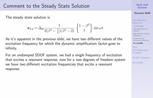
The steady state solution is
xs-s = ∆st1
2(β2 − 12 )(β2 − 2)
{1− β2
1
}sinωt.
As it’s apparent in the previous slide, we have two different values of theexcitation frequency for which the dynamic amplification factor goes toinfinity.
For an undamped SDOF system, we had a single frequency of excitationthat excites a resonant response, now for a two degrees of freedom systemwe have two different excitation frequencies that excite a resonantresponse.
We know how to compute a particular integral for a MDOF system(at least for a harmonic loading), what do we miss to be able todetermine the integral of motion?
Multi DoFSystems
Giacomo Boffi
IntroductoryRemarksAn Example
The Equation ofMotion
Matrices are LinearOperators
Properties ofStructural Matrices
An example
TheHomogeneousProblem
Modal Analysis
Examples
Comment to the Steady State Solution
The steady state solution is
xs-s = ∆st1
2(β2 − 12 )(β2 − 2)
{1− β2
1
}sinωt.
As it’s apparent in the previous slide, we have two different values of theexcitation frequency for which the dynamic amplification factor goes toinfinity.
For an undamped SDOF system, we had a single frequency of excitationthat excites a resonant response, now for a two degrees of freedom systemwe have two different excitation frequencies that excite a resonantresponse.
We know how to compute a particular integral for a MDOF system(at least for a harmonic loading), what do we miss to be able todetermine the integral of motion?

Multi DoFSystems
Giacomo Boffi
IntroductoryRemarks
TheHomogeneousProblemThe HomogeneousEquation of Motion
Eigenvalues andEigenvectors
Eigenvectors areOrthogonal
Modal Analysis
Examples
Homogeneous equation of motion
To understand the behaviour of a MDOF system, we have to studythe homogeneous solution.Let’s start writing the homogeneous equation of motion,
M x+Kx = 0.
The solution, in analogy with the SDOF case, can be written interms of a harmonic function of unknown frequency and, using theconcept of separation of variables, of a constant vector, the so calledshape vector ψ:
x(t) = ψ(A sinωt+B cosωt).
Substituting in the equation of motion, we have(K − ω2M
)ψ(A sinωt+B cosωt) = 0

Multi DoFSystems
Giacomo Boffi
IntroductoryRemarks
TheHomogeneousProblemThe HomogeneousEquation of Motion
Eigenvalues andEigenvectors
Eigenvectors areOrthogonal
Modal Analysis
Examples
Eigenvalues
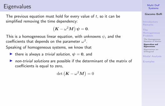
The previous equation must hold for every value of t, so it can besimplified removing the time dependency:(
K − ω2M)ψ = 0.
This is a homogeneous linear equation, with unknowns ψi and thecoefficients that depends on the parameter ω2.
Speaking of homogeneous systems, we know thatI there is always a trivial solution, ψ = 0, andI non-trivial solutions are possible if the determinant of the matrix of
coefficients is equal to zero,
det(K − ω2M
)= 0
The eigenvalues of the MDOF system are the values of ω2 for which theabove equation (the equation of frequencies) is verified or, in other words,the frequencies of vibration associated with the shapes for which
Kψ sinωt = ω2Mψ sinωt.
Multi DoFSystems
Giacomo Boffi
IntroductoryRemarks
TheHomogeneousProblemThe HomogeneousEquation of Motion
Eigenvalues andEigenvectors
Eigenvectors areOrthogonal
Modal Analysis
Examples
Eigenvalues
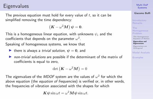
The previous equation must hold for every value of t, so it can besimplified removing the time dependency:(
K − ω2M)ψ = 0.
This is a homogeneous linear equation, with unknowns ψi and thecoefficients that depends on the parameter ω2.Speaking of homogeneous systems, we know thatI there is always a trivial solution, ψ = 0, andI non-trivial solutions are possible if the determinant of the matrix of
coefficients is equal to zero,
det(K − ω2M
)= 0
The eigenvalues of the MDOF system are the values of ω2 for which theabove equation (the equation of frequencies) is verified or, in other words,the frequencies of vibration associated with the shapes for which
Kψ sinωt = ω2Mψ sinωt.
Multi DoFSystems
Giacomo Boffi
IntroductoryRemarks
TheHomogeneousProblemThe HomogeneousEquation of Motion
Eigenvalues andEigenvectors
Eigenvectors areOrthogonal
Modal Analysis
Examples
Eigenvalues
The previous equation must hold for every value of t, so it can besimplified removing the time dependency:(
K − ω2M)ψ = 0.
This is a homogeneous linear equation, with unknowns ψi and thecoefficients that depends on the parameter ω2.Speaking of homogeneous systems, we know thatI there is always a trivial solution, ψ = 0, andI non-trivial solutions are possible if the determinant of the matrix of
coefficients is equal to zero,
det(K − ω2M
)= 0
The eigenvalues of the MDOF system are the values of ω2 for which theabove equation (the equation of frequencies) is verified or, in other words,the frequencies of vibration associated with the shapes for which
Kψ sinωt = ω2Mψ sinωt.
Multi DoFSystems
Giacomo Boffi
IntroductoryRemarks
TheHomogeneousProblemThe HomogeneousEquation of Motion
Eigenvalues andEigenvectors
Eigenvectors areOrthogonal
Modal Analysis
Examples
Eigenvalues, cont.
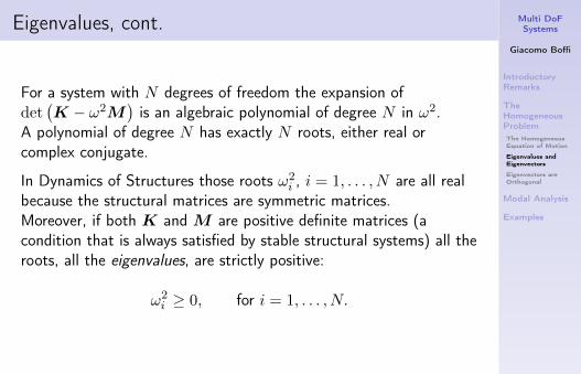
For a system with N degrees of freedom the expansion ofdet(K − ω2M
)is an algebraic polynomial of degree N in ω2.
A polynomial of degree N has exactly N roots, either real orcomplex conjugate.
In Dynamics of Structures those roots ω2i , i = 1, . . . , N are all real
because the structural matrices are symmetric matrices.Moreover, if both K and M are positive definite matrices (acondition that is always satisfied by stable structural systems) all theroots, all the eigenvalues, are strictly positive:
ω2i ≥ 0, for i = 1, . . . , N.
Multi DoFSystems
Giacomo Boffi
IntroductoryRemarks
TheHomogeneousProblemThe HomogeneousEquation of Motion
Eigenvalues andEigenvectors
Eigenvectors areOrthogonal
Modal Analysis
Examples
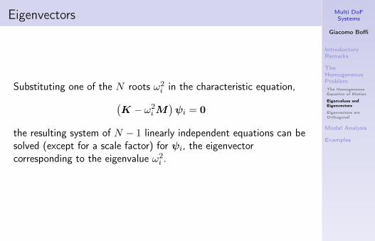
Eigenvectors
Substituting one of the N roots ω2i in the characteristic equation,(
K − ω2iM
)ψi = 0
the resulting system of N − 1 linearly independent equations can besolved (except for a scale factor) for ψi, the eigenvectorcorresponding to the eigenvalue ω2
i .

Multi DoFSystems
Giacomo Boffi
IntroductoryRemarks
TheHomogeneousProblemThe HomogeneousEquation of Motion
Eigenvalues andEigenvectors
Eigenvectors areOrthogonal
Modal Analysis
Examples
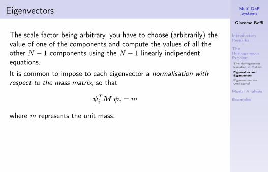
Eigenvectors
The scale factor being arbitrary, you have to choose (arbitrarily) thevalue of one of the components and compute the values of all theother N − 1 components using the N − 1 linearly indipendentequations.
It is common to impose to each eigenvector a normalisation withrespect to the mass matrix, so that
ψTi Mψi = m
where m represents the unit mass.
Please consider that, substituting different eigenvalues in theequation of free vibrations, you have different linear systems,leading to different eigenvectors.
Multi DoFSystems
Giacomo Boffi
IntroductoryRemarks
TheHomogeneousProblemThe HomogeneousEquation of Motion
Eigenvalues andEigenvectors
Eigenvectors areOrthogonal
Modal Analysis
Examples
Eigenvectors
The scale factor being arbitrary, you have to choose (arbitrarily) thevalue of one of the components and compute the values of all theother N − 1 components using the N − 1 linearly indipendentequations.It is common to impose to each eigenvector a normalisation withrespect to the mass matrix, so that
ψTi Mψi = m
where m represents the unit mass.
Please consider that, substituting different eigenvalues in theequation of free vibrations, you have different linear systems,leading to different eigenvectors.

Multi DoFSystems
Giacomo Boffi
IntroductoryRemarks
TheHomogeneousProblemThe HomogeneousEquation of Motion
Eigenvalues andEigenvectors
Eigenvectors areOrthogonal
Modal Analysis
Examples
Initial Conditions
The most general expression (the general integral) for thedisplacement of a homogeneous system is
x(t) =
N∑i=1
ψi(Ai sinωit+Bi cosωit).
In the general integral there are 2N unknown constants ofintegration, that must be determined in terms of the initialconditions.

Multi DoFSystems
Giacomo Boffi
IntroductoryRemarks
TheHomogeneousProblemThe HomogeneousEquation of Motion
Eigenvalues andEigenvectors
Eigenvectors areOrthogonal
Modal Analysis
Examples
Initial Conditions
Usually the initial conditions are expressed in terms of initial displacementsand initial velocities x0 and x0, so we start deriving the expression ofdisplacement with respect to time to obtain
x(t) =
N∑i=1
ψiωi(Ai cosωit−Bi sinωit)
and evaluating the displacement and velocity for t = 0 it is
x(0) =
N∑i=1
ψiBi = x0, x(0) =
N∑i=1
ψiωiAi = x0.
The above equations are vector equations, each one corresponding to asystem of N equations, so we can compute the 2N constants ofintegration solving the 2N equations
N∑i=1
ψjiBi = x0,j ,
N∑i=1
ψjiωiAi = x0,j , j = 1, . . . , N.

Multi DoFSystems
Giacomo Boffi
IntroductoryRemarks
TheHomogeneousProblemThe HomogeneousEquation of Motion
Eigenvalues andEigenvectors
Eigenvectors areOrthogonal
Modal Analysis
Examples
Orthogonality - 1
Take into consideration two distinct eigenvalues, ω2r and ω2
s , andwrite the characteristic equation for each eigenvalue:
Kψr = ω2rMψr
Kψs = ω2sMψs
premultiply each equation member by the transpose of the othereigenvector
ψTs Kψr = ω2
rψTs Mψr
ψTr Kψs = ω2
sψTr Mψs
Multi DoFSystems
Giacomo Boffi
IntroductoryRemarks
TheHomogeneousProblemThe HomogeneousEquation of Motion
Eigenvalues andEigenvectors
Eigenvectors areOrthogonal
Modal Analysis
Examples
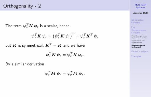
Orthogonality - 2
The term ψTs Kψr is a scalar, hence
ψTs Kψr =
(ψT
s Kψr
)T= ψT
r KT ψs
but K is symmetrical, KT = K and we have
ψTs Kψr = ψT
r Kψs.
By a similar derivation
ψTs Mψr = ψT
r Mψs.

Multi DoFSystems
Giacomo Boffi
IntroductoryRemarks
TheHomogeneousProblemThe HomogeneousEquation of Motion
Eigenvalues andEigenvectors
Eigenvectors areOrthogonal
Modal Analysis
Examples
Orthogonality - 3
Substituting our last identities in the previous equations, we have
ψTr Kψs = ω2
rψTr Mψs
ψTr Kψs = ω2
sψTr Mψs
subtracting member by member we find that
(ω2r − ω2
s) ψTr Mψs = 0
We started with the hypothesis that ω2r 6= ω2
s , so for every r 6= s wehave that the corresponding eigenvectors are orthogonal with respectto the mass matrix
ψTr Mψs = 0, for r 6= s.
Multi DoFSystems
Giacomo Boffi
IntroductoryRemarks
TheHomogeneousProblemThe HomogeneousEquation of Motion
Eigenvalues andEigenvectors
Eigenvectors areOrthogonal
Modal Analysis
Examples
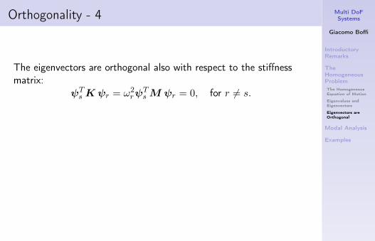
Orthogonality - 4
The eigenvectors are orthogonal also with respect to the stiffnessmatrix:
ψTs Kψr = ω2
rψTs Mψr = 0, for r 6= s.
By definitionMi = ψT
i Mψi
and consequentlyψT
i Kψi = ω2iMi.
Mi is the modal mass associated with mode no. i while Ki ≡ ω2iMi
is the respective modal stiffness.

Multi DoFSystems
Giacomo Boffi
IntroductoryRemarks
TheHomogeneousProblemThe HomogeneousEquation of Motion
Eigenvalues andEigenvectors
Eigenvectors areOrthogonal
Modal Analysis
Examples
Orthogonality - 4
The eigenvectors are orthogonal also with respect to the stiffnessmatrix:
ψTs Kψr = ω2
rψTs Mψr = 0, for r 6= s.
By definitionMi = ψT
i Mψi
and consequentlyψT
i Kψi = ω2iMi.
Mi is the modal mass associated with mode no. i while Ki ≡ ω2iMi
is the respective modal stiffness.

Multi DoFSystems
Giacomo Boffi
IntroductoryRemarks
TheHomogeneousProblem
Modal AnalysisEigenvectors are a base
EoM in ModalCoordinates
Initial Conditions
Examples
Eigenvectors are a base
The eigenvectors are linearly independent, so for every vector x wecan write
x =
N∑j=1
ψjqj .
The coefficients are readily given by premultiplication of x by ψTi M ,
because
ψTi M x =
N∑j=1
ψTi Mψjqj = ψT
i Mψiqi = Miqi
in virtue of the ortogonality of the eigenvectors with respect to themass matrix, and the above relationship gives
qj =ψT
j M x
Mj.

Multi DoFSystems
Giacomo Boffi
IntroductoryRemarks
TheHomogeneousProblem
Modal AnalysisEigenvectors are a base
EoM in ModalCoordinates
Initial Conditions
Examples
Eigenvectors are a base
Generalising our results for the displacement vector to theacceleration vector and expliciting the time dependency, it is
x(t) =
N∑j=1
ψjqj(t), x(t) =
N∑j=1
ψj qj(t),
xi(t) =
N∑j=1
Ψijqj(t), xi(t) =
N∑j=1
ψij qj(t).
Introducing q(t), the vector of modal coordinates and Ψ, theeigenvector matrix, whose columns are the eigenvectors, we can write
x(t) = Ψ q(t), x(t) = Ψ q(t).

Multi DoFSystems
Giacomo Boffi
IntroductoryRemarks
TheHomogeneousProblem
Modal AnalysisEigenvectors are a base
EoM in ModalCoordinates
Initial Conditions
Examples
EoM in Modal Coordinates...
Substituting the last two equations in the equation of motion,
M Ψ q +KΨ q = p(t)
premultiplying by ΨT
ΨTM Ψ q + ΨTKΨ q = ΨTp(t)
introducing the so called starred matrices, with p?(t) = ΨTp(t), wecan finally write
M? q +K? q = p?(t)
The vector equation above corresponds to the set of scalar equations
p?i =∑
m?ij qj +
∑k?ijqj , i = 1, . . . , N.

Multi DoFSystems
Giacomo Boffi
IntroductoryRemarks
TheHomogeneousProblem
Modal AnalysisEigenvectors are a base
EoM in ModalCoordinates
Initial Conditions
Examples
... are N independent equations!
We must examine the structure of the starred symbols.The generic element, with indexes i and j, of the starred matricescan be expressed in terms of single eigenvectors,
m?ij = ψT
i Mψj = δijMi,
k?ij = ψTi Kψj = ω2
i δijMi.
where δij is the Kroneker symbol,
δij =
{1 i = j
0 i 6= j
Substituting in the equation of motion, with p?i = ψTi p(t) we have
a set of uncoupled equations
Miqi + ω2iMiqi = p?i (t), i = 1, . . . , N

Multi DoFSystems
Giacomo Boffi
IntroductoryRemarks
TheHomogeneousProblem
Modal AnalysisEigenvectors are a base
EoM in ModalCoordinates
Initial Conditions
Examples
Initial Conditions Revisited
The initial displacements can be written in modal coordinates,
x0 = Ψ q0
and premultiplying both members by ΨTM we have the followingrelationship:
ΨTM x0 = ΨTM Ψ q0 = M?q0.
Premultiplying by the inverse of M? and taking into account thatM? is diagonal,
q0 = (M?)−1 ΨTM x0 ⇒ qi0 =ψT
i M x0
Mi
and, analogously,
qi0 =ψi
TM x0
Mi

Multi DoFSystems
Giacomo Boffi
IntroductoryRemarks
TheHomogeneousProblem
Modal Analysis
Examples2 DOF System
2 DOF System
k1 = k, k2 = 2k; m1 = 2m, m2 = m;
p(t) = p0 sinωt.
k1
x1 x2
m2
k2
m1
p(t)
x =
{x1x2
}, p(t) =
{0p0
}sinωt,
M = m
[2 00 1
], K = k
[3 −2−2 2
].

Multi DoFSystems
Giacomo Boffi
IntroductoryRemarks
TheHomogeneousProblem
Modal Analysis
Examples2 DOF System
Equation of frequencies
The equation of frequencies is
∥∥K − ω2M∥∥ =
∥∥∥∥3k − 2ω2m −2k−2k 2k − ω2m
∥∥∥∥ = 0.
Developing the determinant
(2m2)ω4 − (7mk)ω2 + (2k2)ω0 = 0
Solving the algebraic equation in ω2
ω21 =
k
m
7−√
33
4ω22 =
k
m
7 +√
33
4
ω21 = 0.31386
k
mω22 = 3.18614
k
m

Multi DoFSystems
Giacomo Boffi
IntroductoryRemarks
TheHomogeneousProblem
Modal Analysis
Examples2 DOF System
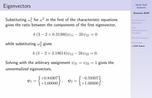
Eigenvectors
Substituting ω21 for ω2 in the first of the characteristic equations
gives the ratio between the components of the first eigenvector,
k (3− 2× 0.31386)ψ11 − 2kψ21 = 0
while substituting ω22 gives
k (3− 2× 3.18614)ψ12 − 2kψ22 = 0.
Solving with the arbitrary assignment ψ21 = ψ22 = 1 gives theunnormalized eigenvectors,
ψ1 =
{+0.84307+1.00000
}, ψ2 =
{−0.59307+1.00000
}.
Multi DoFSystems
Giacomo Boffi
IntroductoryRemarks
TheHomogeneousProblem
Modal Analysis
Examples2 DOF System
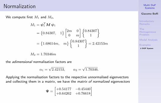
Normalization
We compute first M1 and M2,
M1 = ψT1 Mψ1
={
0.84307, 1}[2m 0
0 m
]{0.84307
1
}={
1.68614m, m}{0.84307
1
}= 2.42153m
M2 = 1.70346m
the adimensional normalisation factors are
α1 =√
2.42153, α2 =√
1.70346.
Applying the normalisation factors to the respective unnormalised eigenvectorsand collecting them in a matrix, we have the matrix of normalized eigenvectors
Ψ =
[+0.54177 −0.45440+0.64262 +0.76618
]

Multi DoFSystems
Giacomo Boffi
IntroductoryRemarks
TheHomogeneousProblem
Modal Analysis
Examples2 DOF System
Modal Loadings
The modal loading is
p?(t) = ΨT p(t)
= p0
[+0.54177 +0.64262−0.45440 +0.76618
] {01
}sinωt
= p0
{+0.64262+0.76618
}sinωt

Multi DoFSystems
Giacomo Boffi
IntroductoryRemarks
TheHomogeneousProblem
Modal Analysis
Examples2 DOF System
Modal EoM
Substituting its modal expansion for x into the equation of motionand premultiplying by ΨT we have the uncoupled modal equation ofmotion {
mq1 + 0.31386k q1 = +0.64262 p0 sinωt
mq2 + 3.18614k q2 = +0.76618 p0 sinωt
Note that all the terms are dimensionally correct. Dividing by mboth equations, we haveq1 + ω2
1q1 = +0.64262p0m
sinωt
q2 + ω22q2 = +0.76618
p0m
sinωt

Multi DoFSystems
Giacomo Boffi
IntroductoryRemarks
TheHomogeneousProblem
Modal Analysis
Examples2 DOF System
Particular Integral
We setξ1 = C1 sinωt, ξ = −ω2C1 sinωt
and substitute in the first modal EoM:
C1
(ω21 − ω2) sinωt =
p?1m
sinωt
solving for C1
C1 =p?1m
1
ω21 − ω2
with ω21 = K1/m ⇒ m = K1/ω
21 :
C1 =p?1K1
ω21
ω21 − ω2
= ∆(1)st
1
1− β21
with ∆(1)st =
p?1K1
= 2.047p0k
and β1 =ω
ω1
of course
C2 = ∆(2)st
1
1− β22
with ∆(2)st =
p?2K2
= 0.2404p0k
and β2 =ω
ω2
Multi DoFSystems
Giacomo Boffi
IntroductoryRemarks
TheHomogeneousProblem
Modal Analysis
Examples2 DOF System
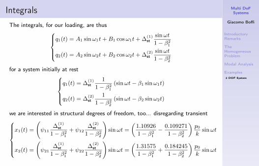
IntegralsThe integrals, for our loading, are thus
q1(t) = A1 sinω1t+B1 cosω1t+ ∆(1)st
sinωt
1− β21
q2(t) = A2 sinω2t+B2 cosω2t+ ∆(2)st
sinωt
1− β22
for a system initially at restq1(t) = ∆
(1)st
1
1− β21
(sinωt− β1 sinω1t)
q2(t) = ∆(2)st
1
1− β22
(sinωt− β2 sinω2t)
we are interested in structural degrees of freedom, too... disregarding transientx1(t) =
(ψ11
∆(1)st
1− β21
+ ψ12∆
(2)st
1− β22
)sinωt =
(1.10926
1− β21
− 0.109271
1− β22
)p0k
sinωt
x2(t) =
(ψ21
∆(1)st
1− β21
+ ψ22∆
(2)st
1− β22
)sinωt =
(1.31575
1− β21
+0.184245
1− β22
)p0k
sinωt

Multi DoFSystems
Giacomo Boffi
IntroductoryRemarks
TheHomogeneousProblem
Modal Analysis
Examples2 DOF System
The response in modal coordinates
To have a feeling of the response in modal coordinates, let’s say that thefrequency of the load is ω = 2ω0, hence β1 = 2.0√
0.31386= 6.37226 and
β2 = 2.0√3.18614
= 0.62771.
-2-1.5
-1-0.5
0 0.5
1 1.5
2 2.5
0 5 10 15 20 25 30
qi/Δ
st
α = ωo t
q1(α)/Δst q2(α)/Δst
In the graph above, the responses are plotted against an adimensional timecoordinate α with α = ω0t, while the ordinates are adimensionalised withrespect to ∆st = p0
k

Multi DoFSystems
Giacomo Boffi
IntroductoryRemarks
TheHomogeneousProblem
Modal Analysis
Examples2 DOF System
The response in structural coordinates
Using the same normalisation factors, here are the response functions interms of x1 = ψ11q1 + ψ12q2 and x2 = ψ21q1 + ψ22q2:
-2-1.5
-1-0.5
0 0.5
1 1.5
2 2.5
0 5 10 15 20 25 30
xi/Δ
st
α = ωo t
x1(α)/Δst x2(α)/Δst