multi-objective optimal sensor deployment under ... library/events/2015/crosscutting... ·...
TRANSCRIPT

Multi-Objective Optimal Sensor Deployment Under Uncertainty for
Advanced Power Systems
Pallabi Sen, Kinnar Sen, and Urmila DiwekarCenter for Uncertain Systems: Tools for Optimization and Management
(CUSTOM)University of Illinois at Chicago
Federal Grant #: DE-FE0011227

Sensor Placement Problem• Advanced Power Systems
– Integrated Gasification Combined Cycle (IGCC)• Objectives
– Determine optimal location of network of sensors– Minimize number of sensors in network– Maximize Efficiency, Maximize Observability, Minimize Cost
• Constraints– Mass and Energy Balances– Environmental factors– Sensor accuracy
2

Main Elements of IGCC Plant
3
Gasification Plant
Air Separation Unit
Syngas Cleanup Process(Radiant Syngas Cooler)
Power Generation Block

Model Uncertainties• Variations to process variables lead directly to variations
in the gasification performance• Plant with no sensors use models to control variations
– Soft sensing– Introduces large errors in control resulting in large variations in
output variables– Reduced observability
• Sensors reduce errors in control• Cost of sensors is linked to errors in sensing
– High cost sensors, less variation– Low cost sensors, high variation
4

Model Uncertainties
5
7.5 8 8.5 9 9.5 10 10.5 11 11.5 12 12.5
softsensing 25% errorlow quality sensors 5% errormedium quality sensors 2% errorhigh quality sensors 1% error

Mixed Integer Nonlinear, Stochastic Optimization Problem
• Determine location of on‐line sensors to maximize observability of system, maximize efficiency subject to budget constraint
• = network of on‐line sensors; • fj,() = level of observability resulting from the
placement of sensor type at location j; • E,( , yj) = efficiency as a nonlinear function of placement of sensor type
at location j
Plant thearound BalancesEnergy and Mass
,...,2,1,,...,2,1,1,0
,...,2,1,1
s.t.
,,max
,
1,
,1 1
,
1 1,,,
1 1,
,
TSjy
Sjy
ByC
yEyf
outj
outT
j
j
T S
jj
T S
jjjj
T S
jjYy
out
outout
j

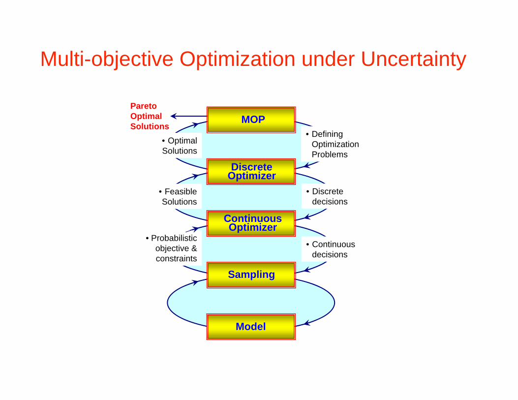
Pareto Optimal Solutions
MOP
Discrete Optimizer
Model
• Discrete decisions
• Optimal Solutions
• Probabilistic objective & constraints
• Defining Optimization Problems
Continuous Optimizer
• Continuous decisions
• Feasible Solutions
Sampling
Multi-objective Optimization under Uncertainty

Optimization under Uncertainty
Stochastic Optimization
Sampling Loop
Optimization Loop
Model
StochasticModeler
Optimizer
OptimalDesign
DecisionVariables
Stochastic Modeling
Sampling Loop
Model
StochasticModeler
OutputCDFs
UncertainVariables

Important Properties of Sampling Techniques• Independence / Randomness• Uniformity
In most applications, the actual relationship between successive points in a sample has no physical significance, hence, randomness of the sample for approximating a uniform distribution is not critical (Knuth, 1973).
Once it is apparent that the uniformity properties are critical to the design of sampling techniques, constrained or stratified sampling becomes appealing (Morgan and Henrion, 1990).

•
•
••
• •
••
•
•
•
••
•
••
•
•
••
•
•
•
••
•
•
•
•
•
• •
•
•
•
•
•
••
•
•
•
•
•
••
•
•
•
• •
•
•
•
•••
•
••
••
•
••
•
•
•
•
•
•
•
•
•
•
••
••
••
•
•
•
••
••
• •
•
•
•
••
•
••
••
x
0.0 0.4 0.8
A: Monte Carlo
•
•••
••
••
•
•
•• •
•
••
•
•
•
•
•
•
•
••
•
•
•
•
•
• •
•
•
•
•
•
••
•
•
•
•
•
•
••
•
•
• •
•
•
•
•••
•
• •
• ••
••
•
••
•
•
•
•
•
•
•
••
••
••
•
•
•
••
••
• •
•
•
•
••
•
••
••
x
0.0 0.4 0.8
B: Latin Hypercube
•
•
••
••
•
• ••
•
•
•
•
•
•
••
•
•
•
••
•
•
•
••
•
•
••
•
•
•
••
••
•
•
• •
••
••
•
•
•
•
•
••
•••
•
•
•
••
••
•
•
•
•
•
•
••
•
••
•
••
•
• •
• •
•
••
••
•
•
•
•
•
•
•
•
••
•
•
x
0.0 0.4 0.8
C: Median Latin Hypercube
•
•
•
•
•
•
•
•
•
•
•
•
•
•
•
•
•
•
•
•
•
•
•
•
•
•
•
•
•
•
•
•
•
•
•
•
•
•
•
•
•
•
•
•
•
•
•
•
•
•
•
•
•
•
•
•
•
•
•
•
•
•
•
•
•
•
•
•
•
•
•
•
•
•
•
•
•
•
•
•
•
•
•
•
•
•
•
•
•
•
•
•
•
•
•
•
•
•
•
•
x
0.0 0.4 0.8
D: Hammersley SequenceWozniakowski-Hammersley

Novel Sampling Technique• Hammersley Sequence Sampling (HSS) based on a
Quasi-random number generator
• HSS sampling is at least 3 to 100 times faster than LHS or MCS.
• HSS is preferred sampling for stochastic modeling and/or stochastic optimization.
HSS LHHS HSS2

Pareto Optimal Solutions
MOP
Discrete Optimizer
Model
• Discrete decisions
• Optimal Solutions
• Probabilistic objective & constraints
• Defining Optimization Problems
Continuous Optimizer
• Continuous decisions
• Feasible Solutions
Sampling
Multi-objective Optimization under Uncertainty

Simulation Technique
• Simulate IGCC process Ns times– Comprehensive plant model in ASPEN Plus environment
– Hammersley sequence sampling used to generate uniform spaced samples across d‐dimensional sample space
• Better Optimization for Nonlinear Uncertain Systems (BONUS) (Sahin and Diwekar, 2004)
13

Better Optimization of Nonlinear Uncertain Systems (BONUS)
14
Stochastic Modeler
Model
SAMPLING LOOP
Cumulative Distribution
Base Case OutputZ(Xi)
Probability DistributionBase Case Input
f (Xi)
probability probability
ReweightingScheme
Changed Input Probability Distribution
probability
Estimated Output Cumulative Distribution
Z(xi)
probability
f (xi)

Model Uncertainties
15
7.5 8 8.5 9 9.5 10 10.5 11 11.5 12 12.5
softsensing 25% error low quality sensors 5% error
medium quality sensors 2% error high quality sensors 1% error
Pareto Optimal Solutions
MOP
Discrete Optimizer
Model
• Discrete decisions
• Optimal Solutions
• Probabilistic objective & constraints
• Defining Optimization Problems
Continuous Optimizer
• Continuous decisions
• Feasible Solutions
Sampling
Multi-objective Optimization under Uncertainty

A Simple Multi-objective Linear Example
Max Z1 = 6x1 + x2Z2 = - x1 + 3x2
subject to:3x1 + 2x2 123x1 + 6x2 24x1 3x1, x2 0

Weighting Method: Max.Y=1*Z1+2*Z2
Objective Space
-4
-2
0
2
4
6
8
10
12
14
0 5 10 15 20 25
Z1
Z2
Max. Z1= 6x1+x2Max. Z2=-x1+3x2
A
B
C
D
E
Pareto set
Z1=6x1+x2 Z2=-x1+3x2A(0,0) 0 0B(3,0) 18 -3C(3,1.5) 19.5 0D(2,3) 15 7E(0,4) 4 12

Weighting Method: Max.Y=1*Z1+2*Z2
Objective Space
-4
-2
0
2
4
6
8
10
12
14
0 5 10 15 20 25
Z1
Z2
Max. Z1= 6x1+x2Max. Z2=-x1+3x2
A
B
C
D
E
Pareto set
Z1=6x1+x2 Z2=-x1+3x2A(0,0) 0 0B(3,0) 18 -3C(3,1.5) 19.5 0D(2,3) 15 7E(0,4) 4 12
2 +
1 +

Comparison of the New MINSOOP Algorithm with the Conventional Method
1
10
100
1000
10000
100000
2 3 4 5
Number of objective functions
Num
ber o
f Opt
imiz
atio
n Pr
oble
ms
solv
ed
Conventional Method
New Method

IGCC Process Flowchart & Sensor Placement
• Generate flowchart to determine downstream variables• Define i,j = 1 (0) if variable j is downstream of variable i• Distribution
21
inS
i i
itjijjt xf
xfyfyf1 0
,0 11

Important Input, Intermediate and Output Variables• Input process variables
– 8 variables, including• Oxygen, coal slurry, air flow rates• Recycled HRSG steam temperature & pressure• Gasifier temperature & pressure
• Intermediate and output process variables– 24 variables, including
• Syngas flow rate, temperature, pressure• CO, CO2 flow rates• Gas turbine combustor, high & low pressure exhaust temperature
• Oxygen, coal, air flow rates into gasifier• Slag & fines flow ratesAugust 16-20, 2010 12th International Conference on
Stochastic Programming22

23
Position\ Accuracy ->1 Gasificer syngas flowrate2 Syngas CO flowrate3 Syngas CO2 flowrate4 Syngas temp.5 Syngas pressure6 LP steam turbine temp.7 Gas turbine burn temp.8 Gas turbine exit temp.9 Gas turbine HP stream temp.10 Gas turbine LP stream temp.11 Gas turbine expand. out temp.12 Oxygen flowrate exit expan.13 Syngas flow solids removal14 Coal slurry flowrate gasifier15 Oxygen flowrate gasifier16 Oxygen flowrate exit ASU17 Acid gas flowrate FUEL118 Gas turbine compre. flowrate19 HP steam turbine flowrate20 Coal feed flow rate 21 Slag from syngas22 Fines from syngas23 Gasifier heat output24 HRSG steam heat output

Sample Space• Ns = 800, uniformly distributed using Hammersley sequence sampling method
• Sensors placed on input variables with six‐sigma variation spanning +/‐20% of the nominal value
• Resulting Fisher information about the downstream variables obtained when no sensors are placed in the network, IYjns(yj) and reweighting
• Resulting efficiency is obtained by reweighting
24
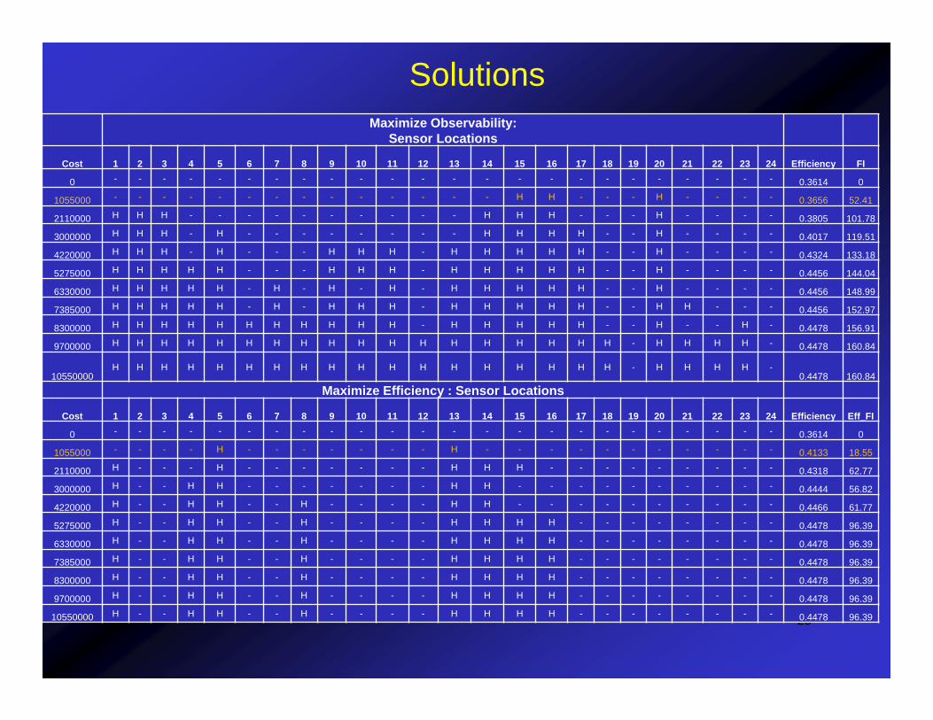
Solutions
25
Maximize Observability:Sensor Locations
Cost 1 2 3 4 5 6 7 8 9 10 11 12 13 14 15 16 17 18 19 20 21 22 23 24 Efficiency FI
0 - - - - - - - - - - - - - - - - - - - - - - - - 0.3614 0
1055000 - - - - - - - - - - - - - - H H - - - H - - - - 0.3656 52.41
2110000 H H H - - - - - - - - - - H H H - - - H - - - - 0.3805 101.78
3000000 H H H - H - - - - - - - - H H H H - - H - - - - 0.4017 119.51
4220000 H H H - H - - - H H H - H H H H H - - H - - - - 0.4324 133.18
5275000 H H H H H - - - H H H - H H H H H - - H - - - - 0.4456 144.04
6330000 H H H H H - H - H - H - H H H H H - - H - - - - 0.4456 148.99
7385000 H H H H H - H - H H H - H H H H H - - H H - - - 0.4456 152.97
8300000 H H H H H H H H H H H - H H H H H - - H - - H - 0.4478 156.91
9700000 H H H H H H H H H H H H H H H H H H - H H H H - 0.4478 160.84
10550000H H H H H H H H H H H H H H H H H H - H H H H -
0.4478 160.84Maximize Efficiency : Sensor Locations
Cost 1 2 3 4 5 6 7 8 9 10 11 12 13 14 15 16 17 18 19 20 21 22 23 24 Efficiency Eff_FI
0 - - - - - - - - - - - - - - - - - - - - - - - - 0.3614 0
1055000 - - - - H - - - - - - - H - - - - - - - - - - - 0.4133 18.55
2110000 H - - - H - - - - - - - H H H - - - - - - - - - 0.4318 62.77
3000000 H - - H H - - - - - - - H H - - - - - - - - - - 0.4444 56.82
4220000 H - - H H - - H - - - - H H - - - - - - - - - - 0.4466 61.77
5275000 H - - H H - - H - - - - H H H H - - - - - - - - 0.4478 96.39
6330000 H - - H H - - H - - - - H H H H - - - - - - - - 0.4478 96.39
7385000 H - - H H - - H - - - - H H H H - - - - - - - - 0.4478 96.39
8300000 H - - H H - - H - - - - H H H H - - - - - - - - 0.4478 96.39
9700000 H - - H H - - H - - - - H H H H - - - - - - - - 0.4478 96.39
10550000 H - - H H - - H - - - - H H H H - - - - - - - - 0.4478 96.39


Conclusions
• Sensor placement in power plant is a stochastic mixed integer nonlinear programming problem
• Novel sampling approach and BONUS algorithm can solve this large scale stochastic programming problem
• Maximize efficiency, maximize observability and minimize cost for good performance coverts the problem into multi‐objective stochastic programming problem
• Novel algorithmic framework can provide solution to this real world problem.
27