multi-procesor systems and scheduling · multiprocessor scheduling – static and dynamic task...
TRANSCRIPT

Interesting topics • Why multiprocessor?
– energy, performance and predictability
• What are multiprocessor systems – Architectures, OS etc
• Design RT systems on multiprocessors – Task Assigment
• Multiprocessor scheduling – (semi-)partitioned scheduling
– global scheduling

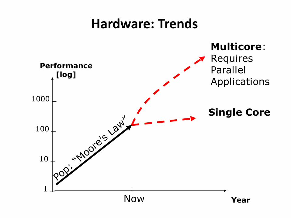
Why multiprocessor systems?
To get high performance and to reduce energy consumption
1
10
100
1000
Now
Performance [log]
Year
Single Core
Multicore: Requires Parallel Applications
Hardware: Trends

Theoretically you may get:
• Higher Performance
– Increasing the cores -- unlimited computing power !
• Lower Power Consumption
– Increasing the cores, decreasing the frequency • Performance (IPC) = Cores * F 2* Cores * F/2 Cores * F
• Power = C * V2 * F 2* C * (V /2)2 * F/2 C * V2 /4 * F
Keep the “same performance” using ¼ of the energy (by doubling the cores)
4
This sounds great for embedded & real-time applications!

What are multiprocessor systems?
“Tightly connected” processors by a “high-speed” interconnect e.g. cross-bar, bus, NoC etc.

6
CPU
L1
CPU
L1
CPU
L1
CPU
L1
CPU
L1
CPU
L1
CPU
L1
CPU
L1
Ban
dw
idth
Typical Multicore Architecture
6
L2 Cache
Off-chip memory

Key Challenges
• New programming models, languages – Ada, Erlang run on multiprocessor systems
• Legacy software migration – Parallelization, synchronization, memory layouts
• New operating systems – Different strategies
• Real-time guarantees for embedded apps – Cache interferences
– Multiprocessor scheduling

mcol cnt mcol mcol mcol sha mcol susane mcol susans
0
50000
100000
150000
200000
250000
300000
350000
Exe
cu
tio
n tim
e (
uS
)
without cache partitioning
An Experiment on a LINUX machine with 2 cores
WCET (vary 10 – 50%)
mcol runs with different programs
8

An Example Architecture
core 1 core 2 core 3 core 4
Private L1 cache
Private L1 cache
Private L1 cache
Private L1 cache
9
Shared L2 cache

Cache analysis on multicore
• L2 cache contents of task 1 may be over-written by task 2
Task 1 Task 2 Task 3 Task 4
10

Cache analysis on multicore
• L2 cache contents of task 1 may be over-written by task 2
Task 1 Task 2 Task 3 Task 4
11

Cache analysis on multicore
Private L1
cache Private L1
cache Private L1
cache Private L1
cache
Shared L2 cache
12
Task 1 Task 2 Task 3 Task 4

Cache-Coloring: partitioning and isolation
Task 1 Task 2 Task 3 Task 4
13

Cache-Coloring: partitioning and isolation
Task 1 Task 2 Task 3 Task 4
14
WCET can be estimated using static techniques for single processor platforms (for the given portion L2 cache)

Cache-Coloring: partitioning and isolation
• E.g. LINUX – Power5 (16 colors)
… …
Logical Pages of Task A Logical Pages of Task B
Physical Pages
… … … …
L2 Cache
controlled by software (OS)
indexed by hardware
15

mcol cnt mcol mcol mcol sha mcol susane mcol susans
0
50000
100000
150000
200000
250000
300000
350000
Exe
cu
tio
n tim
e (
uS
)
without cache partitioning
mcol cnt mcol mcol mcol sha mcol susane mcol susans
0
20000
40000
60000
80000
100000
120000
140000
160000
180000
200000
220000
240000
260000
280000
300000
320000
340000
Exe
cu
tio
n tim
e (
uS
)
with cache partitioning
An Experiment on a LINUX machine with 2 cores
with Cache Coloring/Partitioning [ZhangYi et al]
16

What to do when #tasks > #cores ?
17

The multicore challenge: Schedulability analysis
• #cores < #tasks
Task 1 Task 2 Task 3 Task 4 Task 5
18

Multiprocessor scheduling
• "Given a set J of jobs where job ji has length li and a number of processors mi, what is the minimum possible time required to schedule all jobs in J on
m processors such that none overlap?" – Wikipedia
– That is, design a schedule such that the response time of
the last task is minimized
• The problem is NP-complete
• It is also known as the “load balancing problem”

Multiprocessor scheduling – static and dynamic task assignment
• Partitioned scheduling – Static task assignment
• Each task may only execute on a fixed processor
• No task migration
• Semi-partitioned scheduling – Static task assignment
• Each instance (or part of it) of a task is assigned to a fixed processor
• task instance or part of it may migrate
• Global scheduling
– Dynamic task assignment • Any instance of any task may execute on any processor
• Task migration

Multiprocessor Scheduling
5 2
1 6
8
4
new task
waiting queue
cpu 1 cpu 2 cpu 3
Global Scheduling
cpu 1 cpu 2 cpu 3
5
1
2
8
6
3
9
7
4
cpu 1 cpu 2 cpu 3
2
5
2
1
2 2
3
6
7
4
2 3
Partitioned Scheduling Partitioned Scheduling
with Task Splitting

Global Scheduling
5 2
1 6
8
4
new task
waiting queue
cpu 1 cpu 2 cpu 3
Global Scheduling
• All ready tasks are kept in a global queue
• When selected for execution, a task can be dispatched to any processor, even after being preempted

Global scheduling Algorithms
Any algorithm for single processor scheduling may work, but schedulability analysis is non-trivial
• EDF – Unfortunately not optimal!
– No simple schedulability test known (only sufficient)
• Fixed Priority Scheduling e.g. RM
– Difficult to find the optimal priority order
– Difficult to check the schedulability

Global Scheduling: + and -
• Advantages: – Supported by most multiprocessor operating systems
• Windows NT, Solaris, Linux, ...
– Effective utilization of processing resources (if it works) • Unused processor time can easily be reclaimed at run-time (mixture of hard
and soft RT tasks to optimize resource utilization)
• Disadvantages: – Few results from single-processor scheduling can be used – No “optimal” algorithms known except idealized assumption (Pfair sch) – Poor resource utilization for hard timing constraints
• No more than 50% resource utilization can be guaranteed for hard RT tasks
– Suffers from scheduling anomalies • Adding processors and reducing computation times and other parameters can
actually decrease optimal performance in some scenarios!

Partition-Based Scheduling
cpu 1 cpu 2 cpu 3
5
1
2
8
6
3
9
7
4
Partitioned Scheduling

Bin-packing algorithms
• The problem concerns packing objects of varying sizes in boxes (”bins”) with the objective of minimizing number of used boxes.
– Solutions (Heuristics): Next Fit and First Fit
• Application to multiprocessor systems:
– Bins are represented by processors and objects by tasks.
– The decision whether a processor is ”full” or not is derived from a utilization-based schedulability test.

Partitioned scheduling
• Two steps:
– Determine a mapping of tasks to processors
– Perform run-time scheduling
• Example: Partitioned with EDF
– Assign tasks to the processors such that no processor’s capacity is exceeded (utilization bounded by 1.0)
– Schedule each processor using EDF

Example: Partitioned with RMS Rate-Monotonic-First-Fit (RMFF): [Dhall and Liu, 1978]
• First, sort the tasks in the order of increasing periods.
• Task Assignment
– All tasks are assigned in the First Fit manner starting from the task with highest priority
– A task can be assigned to a processor if all the tasks assigned to the processor are RM-schedulable i.e.
• the total utilization of tasks assigned on that processor is bounded by n(21/n-1) where n is the number of tasks assigned.
(One may also use the Precise test to get a better assignment!)
– Add a new processor if needed for the RM-test.

Partitioned scheduling
• Advantages:
– Most techniques for single-processor scheduling are also applicable here
• Partitioning of tasks can be automated
– Solving a bin-packing algorithm
• Disadvantages:
– Cannot exploit/share all unused processor time
– May have very low utilization, bounded by 50%

Partition-Based Scheduling with Task-Splitting
cpu 1 cpu 2 cpu 3
2
5
2
1
2 2
3
6
7
4
2 3
Partitioned Scheduling with Task Splitting

Partition-Based scheduling with Task Splitting
• High resource utilization
• High overhead (due to task migration)
Fixed-Priority Multiprocessor Scheduling