multidisciplinary system design optimization of fiber
TRANSCRIPT
1
Multidisciplinary System Design Optimization
of Fiber-Optic Networks within Data Centers By
Rany Polany
M.S. Technology and Information Management, University of California, Santa Cruz, 2012
M.B.A., San Diego State University, 2001
M.A. Educational Technology, San Diego State University, 1998
B.S. Cellular and Molecular Biology, San Diego State University, 1996
Submitted to the System Design and Management Program
in Partial Fulfillment of the Requirements for the Degree of
Master of Science in Engineering and Management
at the
MASSACHUSETTS INSTITUTE OF TECHNOLOGY
June, 2016
© 2016 Rany Polany, MMXVI. All Rights Reserved.
The author hereby grants to MIT permission to reproduce and to distribute publicly paper and electronic
copies of this thesis document in whole or in part in any medium now known or hereafter created.
Author: ……………………………………………………………………………………………………
Rany Polany
System Design and Management Program
Certified by: ………………………………………………………………………………………………
Oliver L. de Weck, PhD
Professor of Aeronautics and Astronautics and Engineering Systems
Thesis Supervisor
Certified by: ………………………………………………………………………………………………
Jeremy Kepner, PhD
Lincoln Laboratory Fellow
Thesis Supervisor
Accepted by: ……………………………………………………………………………………………..
Patrick Hale
Senior Lecturer, Engineering Systems Division
Executive Director, System Design and Management Program

2
(THIS PAGE INTENTIONALLY LEFT BLANK)

3
Multidisciplinary System Design Optimization
of Fiber-Optic Networks within Data Centers
By
Rany Polany
Submitted to the System Design and Management Program on May 6, 2016
In Partial Fulfillment of the Requirements for the Degree of
Master of Science in Engineering and Management
Abstract
The growth of the Internet and the vast amount of cloud-based data have created a need to develop data
centers that can respond to market dynamics. The role of a data center designer, whom is responsible for
scoping, building, and managing the infrastructure design is becoming increasingly complex. This work
presents a new analytical systems approach to modeling fiber-optic network design within data centers.
Multidisciplinary system design optimization (MSDO) is utilized to integrate seven disciplines into a
unified software framework for modeling 10G, 40G, and 100G multi-mode fiber-optics networks: 1) market
and industry analysis, 2) fiber-optic technology, 3) data center infrastructure, 4) systems analysis, 5) multi-
objective optimization using genetic algorithms, 6) parallel computing, and 7) simulation research using
MATLAB and OptiSystem. The framework is applied to four theoretical data center case studies to
simultaneously evaluate the Pareto optimal trade-offs of (a) minimizing life-cycle costs, (b) maximizing
user capacity, and (c) maximizing optical transmission quality (Q-factor). The results demonstrate that data
center life-cycle costs are most sensitive to power costs, 10G OM4 multi-mode optical fiber is Pareto
optimal for long reach and low user capacity needs, and 100G OM4 multi-mode optical fiber is Pareto
optimal for short reach and high user capacity needs.
Thesis Supervisor: Oliver L. de Weck, PhD
Title: Professor of Aeronautics and Astronautics and Engineering Systems
Thesis Supervisor: Jeremy Kepner, PhD
Title: Lincoln Laboratory Fellow

4
(THIS PAGE INTENTIONALLY LEFT BLANK)

5
Acknowledgments
To Professor O. de Weck and Dr. J. Kepner, for their direction, thoughts, sharing of industry contacts,
facilitating the collaboration with others to promote my research skills, and the encouragement to pursue
this topic. Thank you.
To the MIT professors that have influenced change in the way I think: S. Eppinger, M. Cusmano, R. de
Neufville, D. Geltner, B. Cameron, E. Crawley, B. Moser, D. Dori, D. Rosenfield, Z. Ton, H. Weil, K.
Wilcox, A. Sanchez, B. Williams, C. Holmes, N. Levenson, F. Murray, L. Perez-Breva, N. Afeyan, D.
Rhodes, S. Saar, M. Davies, and G. Westerman. Thank you.
I am grateful to J. Goodhue at the Massachusetts Green High Performance Computing Center
(MGHPCC) for the tour at the data center and helping me gain an appreciation of a LEED platinum data
center; M. Hubbell at MIT Lincoln Lab for the POD data center tour and research discussions to think about
practical network configurations; M. Silis at MIT Information Systems & Technology for the interview and
discussion about the strategies of forward-thinking in IT planning; A. Hamilton for the interview discussing
Microsoft data center practices and management; K. Bazarnick, Master Engineer, HP POD Systems, for
the tour of the HP POD at the IEEE-HPEC New England conference and the discussions about power and
cooling considerations; and lastly, to K. Friesen for the academics pass to the DataCenter Dynamics 2015
conference in San Francisco, CA, whereby I was able to meet and learn from industry experts. Thank you
for enriching my background with real-world insights.
I extend my gratitude towards two members of OptiWave Incorporated: M. Verreault for the numerous
technical exchanges about using OptiSystem and the help in configuring the simulation frameworks; and
B. Tipper for facilitating the academic licensing.
To the System Design and Management (SDM) program administration team, P. Hale, B. Foley, T.
Nguyen, J. Rubin, J. Pratt, M. Parrillo, N. Gutierrez, D. Schultz, L. Perera, L. Slavin, and D. Erikson, for
operating an exemplary educational platform that has changed me completely. Thank you.
R.Kijewski, thank you for being a great friend and your contributions in helping me think about this
work.
To my wife and daughter, that have sacrificed time together to allow me to further develop myself, my
deepest gratitude. I love you.
This work is dedicated to my children. I hope it serves as inspiration for you to design a meaningful
future.

6
(THIS PAGE INTENTIONALLY LEFT BLANK)

7
Abbreviations and Acronyms APD Avalanche Photodiode
BER Bit Error Rate
CPU Central Processing Unit
dB Decibel
EMBc Calculated Effective Modal Bandwidth
EOR End of Row
Gb Gigabit
Gbps Gigabit per Second
GB Gigabyte
GBps Gigabyte per Second
GFLOPS Giga FLOPS (Floating Point Operations Per Second)
GPU Graphic Processing Unit
HDA Horizontal Distribution Application
HPC High Performance Computing
IP Internet Protocol
ISO International Organization for Standardization
LAN Local Area Network
LEED Leadership in Energy and Environmental Design
MB/s Megabyte per Second
Mbps Megabit per Second
MDA Main Distribution Area
MFD Mode-Field Diameter
MMF Multimode Fiber
MOGA Multi-Objective Genetic Algorithm
MSDO Multi-Disciplinary System Design Optimization
NA Numerical Aperture
NAICS North American Industry Classification System
OM1 Optical Multimode 1
OM2 Optical Multimode 2
OM3 Optical Multimode 3 – Laser Optimized
OM4 Optical Multimode 4 – Laser Optimized
OPD Object-Process Diagram
OPL Object-Process Language
OPM Object-Process Methodology
OS1 Optical Singlemode 1
OS2 Optical Singlemode 2
OSNR Optical Signal to Noise Ratio
OSNR Optical Signal to Noise Ration
PIN Intrinsic Photodiode
PUE Power Usage Effectiveness
Q-factor Ratio of signal power to noise power at the receiver to describe overall system quality.
RX Receiver
SMF Singlemode fiber
SPO Single-Parameter Optimization
TIA-942A Telecommunications Industry Association Standard for Data Centers 942-A
TIR Total Internal Reflections
TOR Top of Rack
TX Transmitter
VCSEL Vertical-Cavity Surface-Emitting Laser
WAN Wide Area Network

8
(THIS PAGE INTENTIONALLY LEFT BLANK)

9
Table of Contents Abstract 3
Acknowledgements 5
Abbreviations and Acronyms 7
Table of Contents 9
Lift of Figures 12
List of Tables 14
1 INTRODUCTION ........................................................................................................................ 15 1.1 MOTIVATION ..................................................................................................................................... 15 1.2 RESEARCH OBJECTIVES ........................................................................................................................ 16 1.3 THESIS STATEMENT ............................................................................................................................. 16 1.4 RESEARCH METHODS .......................................................................................................................... 17
1.4.1 Phase 1: Qualitative analysis ................................................................................................................. 17 1.4.2 Phase 2: Integrated Decision Support Framework ................................................................................ 17 1.4.3 Phase 3: Case Study Analysis ................................................................................................................. 17
1.5 PROBLEM STATEMENT ......................................................................................................................... 18 1.6 SUMMARY OF RESEARCH CONTRIBUTIONS .............................................................................................. 18 1.7 MATRIX OF RELATED WORK ................................................................................................................. 19 1.8 ORGANIZATION OF THE WORK .............................................................................................................. 20
2 THEORY AND INTEGRATED FRAMEWORK .................................................................................. 21 2.1 MARKET ANALYSIS .............................................................................................................................. 21
2.1.1 Data Center: Traffic Classes ................................................................................................................... 21 2.1.2 Regulation and Standards ...................................................................................................................... 22 2.1.3 Growth ................................................................................................................................................... 25 2.1.4 Technology Adoption Life-Cycle (TALC) ................................................................................................. 30 2.1.5 Direction of the Future .......................................................................................................................... 30 2.1.6 The Zettabyte Era—Trends and Analysis ............................................................................................... 31 2.1.7 Summary of Market Analysis ................................................................................................................. 31
2.2 FIBER OPTIC TECHNOLOGY ................................................................................................................... 32 2.2.1 Optical Wave Theory ............................................................................................................................. 32 2.2.2 Optical Fiber Types ................................................................................................................................ 33
2.2.2.1 Overview ....................................................................................................................................... 33 2.2.2.2 Single-Mode .................................................................................................................................. 34 2.2.2.3 Multi-Mode ................................................................................................................................... 34
2.2.3 Optical Bandwidth ................................................................................................................................. 35 2.2.3.1 Index Types ................................................................................................................................... 35 2.2.3.2 EMBc Methodology ....................................................................................................................... 35 2.2.3.3 Bit Error Rate (BER) ....................................................................................................................... 35 2.2.3.4 Q-factor from OSNR ...................................................................................................................... 36
2.2.4 Optical Communication System ............................................................................................................. 37 2.2.4.1 Transmitters .................................................................................................................................. 37 2.2.4.2 Receivers ....................................................................................................................................... 38 2.2.4.3 Bit Error Rate (BER) Analysis ......................................................................................................... 38
2.2.5 Parallel Optics ........................................................................................................................................ 39 2.2.5.1 Experiments Framework ............................................................................................................... 40 2.2.5.2 Power vs. Length ........................................................................................................................... 42 2.2.5.3 Q-factor vs. Length ........................................................................................................................ 46

10
2.2.6 Summary of Fiber Optic Technology ...................................................................................................... 50 2.3 DATA CENTER .................................................................................................................................... 51
2.3.1 Facilities ................................................................................................................................................. 51 2.3.2 Segmented Floor Plan ............................................................................................................................ 52 2.3.3 Data Center Design Considerations ....................................................................................................... 53
2.3.3.1 Tiered Service Levels ..................................................................................................................... 53 2.3.3.2 Power Usage Effectiveness (PUE) ................................................................................................. 54 2.3.3.3 Power Cost Modeling .................................................................................................................... 55 2.3.3.4 Economic comparison of TOR vs. EOR .......................................................................................... 56
2.3.4 Summary of Data Center ....................................................................................................................... 56 2.4 SYSTEMS ANALYSIS ............................................................................................................................. 57
2.4.1 Overview ................................................................................................................................................ 57 2.4.2 Topology ................................................................................................................................................ 58 2.4.3 Hierarchy ................................................................................................................................................ 59
2.4.3.1 Top of Rack (TOR) .......................................................................................................................... 60 2.4.3.2 End of Rack (EOR) .......................................................................................................................... 61
2.4.4 Object-Process Methodology (OPM) and Diagrams (OPD) .................................................................... 63 2.4.5 Summary on Systems Analysis ............................................................................................................... 65
2.5 MOGA: MULTI-OBJECTIVE OPTIMIZATION WITH GENETIC ALGORITHMS..................................................... 66 2.5.1 MSDO: Multi-Disciplinary System Design Optimization Framework ..................................................... 66 2.5.2 Design Variables..................................................................................................................................... 68 2.5.3 Objective Functions ............................................................................................................................... 68 2.5.4 Multi-Objective Optimization ................................................................................................................ 69 2.5.5 Multi-Objective Heuristics with Genetic Algorithms ............................................................................. 70
2.5.5.1 Encoding and Decoding Chromosomes ........................................................................................ 71 2.5.5.2 Initialize Population ...................................................................................................................... 72 2.5.5.3 Fitness ........................................................................................................................................... 72 2.5.5.4 Cross-over ..................................................................................................................................... 72 2.5.5.5 Mutation ....................................................................................................................................... 73 2.5.5.6 Elitistism and Insertion .................................................................................................................. 73
2.5.6 Pareto Front ........................................................................................................................................... 73 2.5.7 Summary of MOGA ................................................................................................................................ 74
2.6 PARALLEL COMPUTING WITH CPU AND GPU .......................................................................................... 75 2.6.1 Vectorized of Functions on the CPU ...................................................................................................... 75 2.6.2 Analysis of Vectorization on Computation Time with CPU .................................................................... 75 2.6.3 Analysis of Vectorized on Computation Time with GPU ........................................................................ 77 2.6.4 CPU versus GPU performance ............................................................................................................... 78 2.6.5 Double vs. Single Precision .................................................................................................................... 78 2.6.6 Summary of Parallel Computing with CPU and GPU.............................................................................. 79
2.7 AN INTEGRATED FRAMEWORK FOR FIBER-OPTIC NETWORK DESIGN ........................................................... 80 2.7.1 Framework Architecture ........................................................................................................................ 80 2.7.2 Flow of Integrated Framework Simulation Operation ........................................................................... 80 2.7.3 Ecosystem and Tools for the Analysis .................................................................................................... 81 2.7.4 Software Dashboard Automation .......................................................................................................... 82 2.7.5 Summary of the Theory and Framework ............................................................................................... 83
3 SIMULATION AND NUMERICAL ANALYSIS .................................................................................. 84 3.1 IMPLEMENTATION APPROACH .............................................................................................................. 84 3.2 PROBLEM FORMULATION ..................................................................................................................... 86 3.3 DEFINITION OF DESIGN VECTORS .......................................................................................................... 86 3.4 GENERALIZED OPTISYSTEM SIMULATION FRAMEWORK FOR STAR TOPOLOGY ............................................... 87 3.5 CASE STUDY SIMULATION PARAMETERS ................................................................................................. 88

11
3.6 CASE 1: 1S.1R.1C.............................................................................................................................. 89 3.6.1 Results .................................................................................................................................................... 89 3.6.2 Discussion .............................................................................................................................................. 90 3.6.3 Observations .......................................................................................................................................... 90
3.7 CASE 2: 1S.1R.10C............................................................................................................................ 91 3.7.1 Results .................................................................................................................................................... 91 3.7.2 Discussions ............................................................................................................................................. 92 3.7.3 Observations .......................................................................................................................................... 92
3.8 CASE 3: 1S.10R.10C ......................................................................................................................... 93 3.8.1 Results .................................................................................................................................................... 93 3.8.2 Discussions ............................................................................................................................................. 94 3.8.3 Observations .......................................................................................................................................... 94
3.9 CASE 4: 2S.10R.10C ......................................................................................................................... 95 3.9.1 Results .................................................................................................................................................... 95 3.9.2 Discussion .............................................................................................................................................. 96 3.9.3 Observations .......................................................................................................................................... 96
3.10 SENSITIVITY ANALYSIS ......................................................................................................................... 97 3.10.1 Framework ............................................................................................................................................. 97 3.10.2 Facility Costs, Power Costs, and PUE ..................................................................................................... 97 3.10.3 Genetic Algorithm Parameters .............................................................................................................. 99
3.11 SUMMARY OF SIMULATION AND NUMERICAL ANALYSIS .......................................................................... 100
4 CONCLUSION AND RECOMMENDATIONS ................................................................................ 101 4.1 Q1: WHAT ARE THE KEY ATTRIBUTES NEEDED TO BUILD A DATA CENTER FIBER-OPTIC NETWORK? ................... 101 4.2 Q2: WHAT ARE THE IMPORTANT FACTORS FOR CONSIDERING PARETO OPTIMAL DATA CENTER FIBER-OPTIC
NETWORKS? ............................................................................................................................................. 102 4.3 Q3: HOW SHOULD DATA CENTER VENDOR’S BEST RESPOND TO NEW TECHNOLOGY PLATFORMS? ................... 103 4.4 Q4: HOW CAN DATA CENTER PROVIDERS ADDRESS FUTURE COMMODITIZATION OF THE INFRASTRUCTURE? ..... 103 4.5 Q5: WHAT SKILLS WILL BE IMPORTANT FOR THE FUTURE-OF-WORK TO MANAGE DATA CENTER SERVICES? ....... 104 4.6 Q6: WHAT IS THE NEXT PHASE OF EVOLUTION FOR DATA CENTER OPTICAL NETWORK DESIGN? ...................... 104 4.7 SUMMARY OF CONTRIBUTIONS ........................................................................................................... 106 4.8 FUTURE WORK................................................................................................................................. 107
5 APPENDIX ............................................................................................................................... 108 5.1 MATLAB CODE ............................................................................................................................... 108
5.1.1 function Optimize_Callback ................................................................................................................. 108 5.1.2 function [LCC] = computeLCC .............................................................................................................. 129 5.1.3 function[Capacity] = computeCapacity ................................................................................................ 131 5.1.4 function [Qfactor] = computeQfactor .................................................................................................. 132 5.1.5 function [Population] = int_pop .......................................................................................................... 133 5.1.6 function [mutationChildren] = int_mutation ....................................................................................... 134 5.1.7 function [xoverKids] = int_crossoverarithemtic................................................................................... 135
6 REFERENCES ........................................................................................................................... 136

12
Table of Figures FIGURE 1.1: MULTI-OBJECTIVE GOALS FOR FIBER-OPTIC NETWORK PLANNING ................................. 15
FIGURE 1.2: REPRESENTATION OF THE PROBLEM STATEMENT ................................................................. 18
FIGURE 2.1: SUMMARY OF THE LITERATURE REVIEW ................................................................................. 21
FIGURE 2.2: BROAD CLASSES OF TRAFFIC FLOW ........................................................................................... 21
FIGURE 2.3: FOUR LEVELS OF LEED CERTIFICATION .................................................................................... 23
FIGURE 2.4: TIA-942 TELECOMMUNICATIONS DATA CENTER INFRASTRUCTURE STANDARD .......... 24
FIGURE 2.5: DENSITY OF DATA CENTER FACILITIES (CONUS, N=1133) ..................................................... 25
FIGURE 2.6: DENSITY OF BROADBAND, WEIGHTED BY DOWNLOAD SPEED (CONUS, N=5758) .......... 25
FIGURE 2.7: LEVEL3 COMMUNICATIONS INC. FIBER OPTIC NETWORK .................................................... 27
FIGURE 2.8: US COUNTY & ZIP CODE BUSINESS PATTERNS: NAICS 518210 ............................................. 28
FIGURE 2.9: MAGIC QUADRANT FOR CLOUD INFRASTRUCTURE AS A SERVICE ................................... 28
FIGURE 2.10: HYPE CYCLE FOR COMMUNICATIONS SERVICE PROVIDER INFRASTRUCTURE, 2014 . 29
FIGURE 2.11: TECHNOLOGY ADOPTION LIFE-CYCLE ANALYSIS OF BROADBAND TECHNOLOGY.... 30
FIGURE 2.12: FIBER-OPTIC MARKET DECOMPOSITION (TOP VIEW) ........................................................... 30
FIGURE 2.13: CISCO VNI FORECASTS 168 EXABYTES PER MONTH OF IP TRAFFIC BY 2019.................. 31
FIGURE 2.14: MODE-FIELD DISTRIBUTION ........................................................................................................ 32
FIGURE 2.15: TOTAL INTERNAL REFLECTIONS ............................................................................................... 32
FIGURE 2.16: NUMERICAL APERTURE................................................................................................................ 32
FIGURE 2.17: ATTENUATION ................................................................................................................................ 32
FIGURE 2.18: DISPERSION ...................................................................................................................................... 32
FIGURE 2.19: COMPARISON OF OPTICAL FIBER CROSS-SECTIONS ............................................................. 33
FIGURE 2.20: COMPARISON OF OPTICAL FIBER INTERNAL LIGHT TRAVEL PATH ................................. 33
FIGURE 2.21: BIT ERROR RATE VERSUS Q-FACTOR ........................................................................................ 36
FIGURE 2.22: FIBER-OPTIC COMMUNICATION SYSTEM DESIGN ................................................................. 37
FIGURE 2.23: TRANSMITTER COMPONENTS ..................................................................................................... 37
FIGURE 2.24: RECEIVER COMPONENTS ............................................................................................................. 38
FIGURE 2.25: BIT ERROR RATE (BER) ANALYZER AT Q ≈ 7 ........................................................................... 38
FIGURE 2.26: 40G AND 100G PARALLEL OPTICS .............................................................................................. 39
FIGURE 2.27: FRAMEWORK FOR PARALLEL OPTICS EXPERIMENTS .......................................................... 40
FIGURE 2.28: OPTISYSTEM SINGLE-PARAMETER OPTIMIZATION (SPO) TO Q-FACTOR= 7±.1 .............. 41
FIGURE 2.29: EXAMPLE OF OPTISYSTEM VISUALIZATION REPORT OUTPUT .......................................... 41
FIGURE 2.30: 10G OM3: POWER (DBM) VERSUS Q-FACTOR ........................................................................... 42
FIGURE 2.31: 10G OM4: POWER (DBM) VERSUS Q-FACTOR ........................................................................... 43
FIGURE 2.32: 40G OM3: POWER (DBM) VERSUS Q-FACTOR ........................................................................... 43
FIGURE 2.33: 40G OM4: POWER (DBM) VERSUS Q-FACTOR ........................................................................... 44
FIGURE 2.34: 100G OM3: POWER (DBM) VERSUS Q-FACTOR ......................................................................... 44
FIGURE 2.35: 100G OM4: POWER (DBM) VERSUS Q-FACTOR ......................................................................... 45
FIGURE 2.36: 10G OM4 VS. OM3: Q-FACTOR VERSUS LENGTH ..................................................................... 46
FIGURE 2.37: 40G OM4 VS. OM3: Q-FACTOR VERSUS LENGTH ..................................................................... 47
FIGURE 2.38: 100G OM4 VS. OM3: Q-FACTOR VERSUS LENGTH ................................................................... 48
FIGURE 2.39: GENERIC DATA CENTER FACILITIES DIAGRAM ..................................................................... 51
FIGURE 2.40: GENERIC REPRESENTATION OF A DATA CENTER FLOOR PLAN ........................................ 52
FIGURE 2.41: TIA-942 DATA CENTER INFRASTRUCTURE REDUNDANCY TOPOLOGY ........................... 53
FIGURE 2.42: A BREAKDOWN OF DATACENTER ENERGY OVERHEAD COSTS ........................................ 54

13
FIGURE 2.43: MAPPING FUNCTION TO FORM ................................................................................................... 57
FIGURE 2.44: SYSTEMS ANALYSIS PROCESS (TOPOLOGY>HIERARCHY>OPM) ....................................... 57
FIGURE 2.45: GENERIC FORMAT FOR A TOPOLOGICAL REPRESENTATION ............................................. 58
FIGURE 2.46: TIA-942 STAR TOPOLOGY ............................................................................................................. 58
FIGURE 2.47: A GENERALIZED HIERARCHICAL DECOMPOSITION ............................................................. 59
FIGURE 2.48: HIERARCHICAL ARCHITECTURE OF A MULTI-TIER DATA CENTER .................................. 59
FIGURE 2.49: RACK LAYOUT AND POWER REQUIREMENTS ........................................................................ 60
FIGURE 2.50: TOR CONFIGURATION ................................................................................................................... 60
FIGURE 2.51: 144-CABINET TOR CONFIGURATION IN A DATA CENTER .................................................... 61
FIGURE 2.52: EOR CONFIGURATION ................................................................................................................... 61
FIGURE 2.53: 144-CABINET EOR CONFIGURATION IN A DATA CENTER .................................................... 62
FIGURE 2.54: GENERIC FORMAT FOR AN OPD REPRESENTATION .............................................................. 63
FIGURE 2.55: OPD OF A DATA CENTER REPRESENTING PROCESS PROJECTED ONTO FORM .............. 64
FIGURE 2.56: MULTIDISCIPLINARY SYSTEM DESIGN OPTIMIZATION FRAMEWORK ............................ 66
FIGURE 2.57: CONSIDERING CHALLENGES OF INCREASING COMPUTATIONAL DIFFICULTY ............ 67
FIGURE 2.58: GLOBAL MAX AND GLOBAL MIN OF THE PEAKS OBJECTIVE FUNCTION ....................... 69
FIGURE 2.59: MAPPING CHROMOSOMES TO BINARY ..................................................................................... 70
FIGURE 2.60: PROCEDURE FOR GENETIC ALGORITHM.................................................................................. 71
FIGURE 2.61: GENETIC ALGORITHM CROSS-OVER ......................................................................................... 72
FIGURE 2.62: GENETIC ALGORITHM MUTATION ............................................................................................. 73
FIGURE 2.63: EXAMPLE OF A PARETO FRONTIER ........................................................................................... 73
FIGURE 2.64: IMPACT OF THREE VECTORIZATION APPROACHES ON CPU COMPUTATION TIME ...... 75
FIGURE 2.65: GPU DATA TRANSFER BANDWIDTH (NVIDIA GTX970) ......................................................... 77
FIGURE 2.66: ACHIEVED PEAK READ+WRITE AND CALCULATION RATES WITH GPU VERSUS CPU . 78
FIGURE 2.67: DOUBLE VS. SINGLE PRECISION WITH GPU COMPUTING .................................................... 79
FIGURE 2.68: MSDO FRAMEWORK APPLIED TO FIBER-OPTIC NETWORK DESIGN ................................. 80
FIGURE 2.69: FLOW OF FRAMEWORK OPERATION ......................................................................................... 80
FIGURE 2.70: ECOSYSTEM AND TOOLS FOR NUMERICAL ANALYSIS ........................................................ 81
FIGURE 2.71: SOFTWARE DASHBOARD ............................................................................................................. 82
FIGURE 3.1: NESTED IMPLEMENTATION APPROACH ..................................................................................... 84
FIGURE 3.2: INPUT AND OUTPUT OF THE MODEL ........................................................................................... 86
FIGURE 3.3: BI-DIRECTIONAL MULTI-MODE FIBER OPTIC STAR TOPOLOGY NETWORK ..................... 87
FIGURE 3.4: CASE STUDY 1 INPUTS AND PARETO FRONTIER RESULTS .................................................... 89
FIGURE 3.5: CASE STUDY 2 INPUTS AND PARETO FRONTIER RESULTS .................................................... 91
FIGURE 3.6: CASE STUDY 3 INPUTS AND PARETO FRONTIER RESULTS .................................................... 93
FIGURE 3.7: CASE STUDY 4 INPUTS AND PARETO FRONTIER RESULTS .................................................... 95
FIGURE 3.8: PARAMETERS EXPLORED FOR SENSITIVITY ANALYSIS ........................................................ 97
FIGURE 3.9: SENSITIVITY ANALYSIS FOR FACILITY COSTS, POWER COSTS, AND PUE ........................ 97
FIGURE 3.10: SENSITIVITY ANALYSIS FOR BANDWIDTH PER USER [10, 20, 30, 40, 50] MB/S ................ 98
FIGURE 4.1: DATA CENTER MESH FABRIC ...................................................................................................... 105

14
Table of Tables TABLE 1.1: NOTATION FOR PROBLEM STATEMENT ....................................................................................... 18
TABLE 1.2: SUMMARY MATRIX OF THE LITERATURE REVIEW .................................................................. 19
TABLE 2.1: CITIES WITH HIGHEST DATA CENTER DENSITY AND CITIES WITH FASTEST INTERNET
SPEEDS .............................................................................................................................................................. 26
TABLE 2.2: SINGLE-MODE FIBER-OPTIC CHARACTERISTICS ....................................................................... 34
TABLE 2.3: MULTI-MODE FIBER-OPTIC CHARACTERISTICS ........................................................................ 34
TABLE 2.4: OM3 VS. OM4: POWER AT MAX DISTANCE, OPTIMIZED FOR Q = 7 ........................................ 45
TABLE 2.5 OM3: EQUATIONS FOR Q-FACTOR VS. LENGTH (TX POWER (DBM) Q = 7 ± .1 AT MAX
DISTANCE) ....................................................................................................................................................... 49
TABLE 2.6: OM4: EQUATIONS FOR Q-FACTOR VS. LENGTH (TX POWER (DBM) Q = 7 ± .1 AT MAX
DISTANCE) ....................................................................................................................................................... 49
TABLE 2.7: SUMMARY OF DATA CENTER INFRASTRUCTURE COMPONENTS ......................................... 51
TABLE 2.8: OPTICAL COMPONENTS IN A DATA CENTER FLOOR PLAN ..................................................... 52
TABLE 2.9: DATA CENTER REDUNDANCY TIER LEVELS .............................................................................. 54
TABLE 2.10: TOR VS. EOR: ECONOMIC COMPARISON OF LOW AND HIGH DENSITY (144 SERVER
CABINETS) ....................................................................................................................................................... 56
TABLE 2.11: PROS AND CONS OF TOP OF RACK (TOR) ................................................................................... 61
TABLE 2.12: PROS AND CONS OF END OF RACK (EOR) .................................................................................. 62
TABLE 2.13: OPL SPECIFICATION FOR A DATA CENTER ............................................................................... 65
TABLE 2.14: NOTATION FOR NUMBER TYPES .................................................................................................. 68
TABLE 2.15: PERFORMANCE OF A VECTORIZED GA FOR AN OBJECTIVE FUNCTION USING
GAOPTIONSDEMO ........................................................................................................................................... 76
TABLE 2.16: AMAZON EC2 INSTANCES GPU VERSUS CPU ............................................................................ 78
TABLE 2.17: GPU: DATA-TYPE PRECISION GIGAFLOPS ................................................................................. 79
TABLE 2.18: DESCRIPTION OF SOFTWARE TOOLS FOR THE NUMERICAL ANALYSIS ........................... 81
TABLE 3.1: SUMMARY OF THE STEP-WISE APPROACH FOR CASE STUDIES ............................................ 84
TABLE 3.2: MAX DISTANCE FOR SINGLE-PARAMETER OPTIMIZATION OF POWER TO Q-FACTOR = 7
± .1 ...................................................................................................................................................................... 85
TABLE 3.3: CASE STUDY PARAMETERS............................................................................................................. 88
TABLE 3.4: SENSITIVITY ANALYSIS FOR FACILITY COSTS, POWER COSTS, AND PUE .......................... 97
TABLE 3.5: SENSITIVITY ANALYSIS OF GENETIC ALGORITHM POPULATION SIZE ON CPUTIME ...... 99
TABLE 3.6: SENSITIVITY ANALYSIS OF GENETIC ALGORITHM GENERATIONS ON CPUTIME ............ 99
TABLE 3.7: SUMMARY OF CASE STUDY DATA CENTER COSTS (%).......................................................... 100
TABLE 3.8: SUMMARY OF PARETO FRONTIER FREQUENCY FOR SENSITIVITY OF BANDWIDTH PER
USER ................................................................................................................................................................ 100

15
1 Introduction
At the time of writing this work, the US President has signed a new executive order, referred to as the
National Strategic Computing Initiative (NSCI) [1], to build an exascale super-computer system [2]. The
primary mandate of the NSCI initiative is to: “Establish hardware technology for future High-Performance
System (HPC) systems.” It is the goal of this thesis to make a contribution in this field by considering a
new multi-disciplinary and systems approach towards the design of the fiber-optic intra-connection network
within data centers for the HPC systems to enable the optimized transport of data.
1.1 Motivation
The growth of the Internet and the vast amount of cloud-based data has created a need to build data centers
that can respond to market, customer and technology dynamics, which includes: variability in demand,
capacity planning, commoditization of hardware and services, globally accessible customers, political
influences, and advances in new technology. The role of a decision maker, whom is responsible for scoping,
building, and managing the data center infrastructure design is becoming increasingly complex. Yet, the
practical resources for gaining insights into the possible design options are lacking; only those with
exceptional computational and critical analytical skills are able to develop the foresight for the planning
options. As shown by a 2005 Massachusetts Institute of Technology (MIT) data center planning study [3],
the approaches to future data center design requires new ways of thinking about trade-offs and planning. In
this work, I consider at a broad level, the data center design, and more specifically, the optical network
within a data center.
Figure 1.1: Multi-Objective Goals for Fiber-Optic Network Planning

16
Shown in Figure 1.1 above is an example of a representation of three business dimensions that a
business decision manager might consider when planning for a fiber-optic network. In the provided
example, the x-axis is tracking the Capacity of the system in terms of simultaneous users; the y-axis is
tracking the Costs ($); and the z-axis is tracking the Optical Transmission Quality in terms of Q-factor, a
ratio of optical signal to noise estimation. The ‘Current’ vector represents the performance state of a current
system and the ‘Goal’ vector represents the desired outcome of an implementation; in the provided example,
the goal for Cost reduction is 30%, the Optical transmission quality is improved by 10%, and the Capacity
increased by 20%. Performing this type of multi-objective goal mapping empowers the decision maker to
understand the overall business direction and the potential changes required to the system life-cycle, which
are not myopically focused on one aspect. The Utopia point represents the ideal (yet hypothetical) state,
which in the example of Figure 1.1 above would represent zero optical loss, zero cost, and unlimited users—
clearly not feasible, but worthwhile to consider in which direction and magnitude the decision maker should
be optimizing the objectives.
1.2 Research Objectives
The main objective of this work is to develop a new and improved approach to modeling data center fiber-
optic infrastructures system designs that can be used to address the following business operations concerns:
1. What are the key attributes needed to build a data center fiber-optic network?
2. What are the important factors for considering Pareto optimal data center fiber-optic networks?
3. How should data center vendor’s best respond to new technology platforms?
4. How can data center providers address future commoditization of the infrastructure?
5. What skills will be important for the future-of-work to manage data center services?
6. What is the next phase of evolution for data center optical network design?
This work yields a practical decision support framework and computational process that can model the
key parameters of a data center fiber-optic systems network design and facilitate a decision manager’s
ability to analytically consider the long-term life-cycle planning of resources.
1.3 Thesis statement
Utilizing a multidisciplinary systems design optimization (MSDO) [4] approach by integrating fiber-optic
technology, systems-based analysis, multi-objective genetic algorithms, and parallel computation, provides
enhanced insight towards considering trade-offs for minimizing life-cycle costs, maximizing capacity, and
maximizing optical network performance of data center fiber-optic infrastructure design.

17
1.4 Research Methods
This work is divided into three phases: 1) Qualitative analysis consisting of interviews and background
literature review, 2) Development of an integrated framework which builds up the framework and modeling
approach, and 3) Case study analysis which explores four different ecosystems.
1.4.1 Phase 1: Qualitative analysis
A literature review of published information develops the underlying theory and approach for the thesis.
Industry experts are interviewed to learn about the evolution of the data center and to understand more
about the short-term and long-term concerns. The goal of this phase is to synthesize the background review
and ascertain the design parameters to consider.
1.4.2 Phase 2: Integrated Decision Support Framework
Utilizing a holistic and integrative approach, the output of this phase is a new framework for engineers and
management to use towards making practical decisions about data centers fiber-optic network design. The
framework is developed using multi-objective genetic algorithms [5], and implemented in MATLAB [6]
and OptiSystem [7]. The new software framework enables a decision-maker to run simulations and gain
new insights about data center costs and optical network design.
1.4.3 Phase 3: Case Study Analysis
In this phase, four theoretical case studies, which increase in complexity, will be analyzed to determine
which parameters are most important towards system life-cycle costs, user capacity, and optical
performance. This work applies the integrated decision support framework as follows:
A) Case Study 1: One cabinet within a data center (1 Cabinet).
B) Case Study 2: One row of 10 cabinets within a data-center (10 Cabinets).
C) Case Study 3: 10 rows of 10 cabinets within a data center (100 Cabinets).
D) Case Study 4: Two sections of 10 rows of 10 cabinets within a data center (200 Cabinets).
The generalization behind utilizing the four configurations is to emulate potential groupings of cabinets,
also known as Pods, and allow a data center manager to evaluate different potential designs.

18
1.5 Problem Statement
Table 1.1: Notation for Problem Statement
𝑶𝑻𝒊 ≜ Fiber-optic from Optical Transmitter
𝑻𝑭𝒋 ≜ Fiber-optic from Optical Transmitter
𝑶𝑹𝒌 ≜ Fiber-optic from Optical Transmitter
𝑴𝒍 ≜ Optical Switch
𝑫𝒏 ≜ Optical Switch
𝑹 ≜ Data Rate Requirement
𝑻𝑳𝑪 ≜ Total Lifecycle Cost
𝑼𝑪 ≜ User Capacity
𝑶𝑻𝑸 ≜ Optical Transmission Quality
The problem statement, represented visually in Figure 1.2 below, is defined as:
How should 𝑂𝑇𝑖, 𝑇𝐹𝑗, 𝑂𝑅𝑘, 𝑀𝑙, and 𝐷𝑛, be sized (a) and chosen (b), such that the data rate requirement 𝑅
of the network is met, while minimizing total cost (𝑇𝐿𝐶), maximizing user capacity (𝑈𝐶), and maximizing
optical transmission quality (𝑂𝑇𝑄).
Figure 1.2: Representation of the Problem Statement
Adapted from [8], [9]
1.6 Summary of Research Contributions
This work provides a new approach to consider fiber-optic network systems design within data centers by:
1) Developing and presenting a new multidisciplinary system design optimization (MSDO)
approach to considering multiple business objectives.
2) Defining a process to perform simulation using the new integrated MSDO approach.
3) Using the new approach to yield a Pareto front output to aid the decision manager towards
developing an optimal strategy for system life-cycle planning.
Utilizing the approach developed in this work can help address the following business operational concerns:
1) What are the trade-offs between life-cycle cost, system capacity, and optical system quality?
2) What are the most sensitive parameters in the analysis?

19
1.7 Matrix of Related Work
Presented in Table 1.2 below is a matrix which systematically categorizes the literature that have influenced
this thesis. The matrix is categorized horizontally by subject discipline and vertically by research topic. The
numeric format of each citation, [##], is mapped to the Bibliography in Section 5.1.7.
Table 1.2: Summary Matrix of the Literature Review
Subject
Discipline
Research
Topics
Fiber-Optic
Network
Systems
Data Centers Systems
Analysis
Multi-
Objective
Optimization
with Genetic
Algorithms
Parallel
Computing
Simulation
Tools
Introduction [1][2][8][9] [2][3] [4][9] [4][5] [2] [6][7][8]
Market
Analysis
[10][11][12]
[13][14][15]
[16][17][18]
[19][20][21]
[22][23][24]
[25][26][27]
[28][29][30]
[3][31][32]
[33][34][35]
Topology [36][37][38] [39][40][41]
[96][97]
[42][43][44][45]
[46][47][48][49]
[49][50][51][52]
[53][54][55][56]
[57][58][59][60]
[61][62][63][64]
[65][66][67][68]
[69]
Hierarchy [47][48][70]
[71][72]
[71][73][74][75]
[76]
OPM [42][73][77]
Design
Optimization
[78][79][80]
[81][82][83] [3] [84]
[4][6][84][85]
[86][87][88]
[89][90]
Genetic
Algorithms
[4][5][6][87]
[89][91][92]
[93][94][95]
[96][97][98]
Sensitivity
Analysis [4][6]
Pareto
Frontier [4][6]
GPU
Computing
[99][100][101]
[102][103]
Vectorized
Functions
[86][91][92]
[104][105]
[106][107]
CPU vs.
GPU
[91][92][108]
[109]
OptiSystem [7][110][111] [110][111]
MATLAB [6][8] [85] [8][103]
Conclusion [112][113][114][115][116][117][118][119][120][121]

20
1.8 Organization of the Work
Section 2 presents the literature review of the requisite background information and discussion about the
prior research that have influenced the integrated framework developed in this work. Section 3 presents the
implementation of the work with a discussion of the problem statement, problem formulation, definition of
the design vector, definition of the simulation model, representation of the ecosystem and tools for the
analysis, and presents the numerical case study analysis with Pareto front analysis. Lastly, Section 4
presents the conclusions and a discussion about the findings, insights, and recommendations to the future
of data center optical network system.

21
2 Theory and Integrated Framework
The review of the literature synthesizes seven disciplines domains into an integrated framework:
1. Market and industry analysis;
2. Fiber optic technology;
3. Data Center Infrastructure;
4. Systems analysis;
5. Multi-objective optimization using genetic algorithms;
6. Parallel computing; and
7. Simulation research and tools using MATLAB and OptiSystem
Figure 2.1: Summary of the Literature Review
The literature review and corresponding theories for each subject domain is presented independently in the
subsequent sub-sections. The value this section provides is that it extracts the theories from the literature
review and sets up the basis for the integrated software tool in Section 2.7.4 below.
2.1 Market Analysis
There are several important aspects to understand about the role of fiber-optics and the influence the US
domestic market has on the growth of this technology. In the following Sections 2.1.1 - 2.1.7, is a discussion
about the market drivers for fiber-optics telecommunications.
2.1.1 Data Center: Traffic Classes
Figure 2.2: Broad Classes of Traffic Flow
Source: [33]

22
Driven by the large market demand for "Within Data Center” (76%) connectivity, as shown in Figure 2.2
above, the interest of this work to develop a better understanding of the challenges and make a contribution
to a new approach to helping improve the overall efficiency of data center operations.
2.1.2 Regulation and Standards
There are several regulatory and standards organizations that currently drive the regulation of data centers.
These standards are important to understand because they drive the infrastructure design considerations:
Hardware Safety:
Optical lasers standards for safety are defined by the International Electrotechnical Commission (IEC). The
standards for the cables, which include fire safety for building codes and electrical interference are managed
by the Underwriters Laboratories (UL) and Restriction of the Use of Certain Hazardous Substances in
Electrical and Electronic Equipment (RoHS).
SSAE16 Compliance:
These standards provide guidance to external auditors on Generally Accepted Auditing Standards (GAAS)
in regards to auditing an entity and issuing a report.” [10] [11]
ISO Certification:
“ISO (International Organization for Standardization) is an independent, non-governmental membership
organization and the world's largest developer of voluntary International Standards. It is made up of over
162 member countries who are the national standards bodies around the world, with a Central Secretariat
that is based in Geneva, Switzerland. ISO International Standards ensure that products and services are safe,
reliable and of good quality. For business, they are strategic tools that reduce costs by minimizing waste
and errors and increasing productivity. They help companies to access new markets, level the playing field
for developing countries and facilitate free and fair global trade.”[12]
LEED Certification:
“LEED certification is the most widely recognized, and widely used, green building program across the
globe. LEED is a certification program for buildings, homes and communities that guides the design,
construction, operations and maintenance. More than 54,000 projects are currently participating in LEED,
comprising more than 10.1 billion square feet of space. There are four levels of certification - the number
of points a project earns determines the level of LEED certification that the project will receive. Shown in
Figure 2.3 below are the typical certification thresholds: Certified, Silver, Gold, and Platinum.” [13]

23
Figure 2.3: Four Levels of LEED Certification
Source: [13]
Uptime Institute:
“Uptime Institute is recognized globally for the creation and administration of the Tier Standards &
Certifications for Data Center Design, Construction, and Operational Sustainability along with its
Management & Operations reviews, FORCSS™ methodology, and energy efficiency initiatives.” [14]
Telecom Infrastructure Standard for Data Center:
“Standards projects and technical documents initiated by TIA's engineering committees are formulated
according to the guidelines established by the TIA Engineering Committee Operating Procedures (ECOP)
and the ANSI Essential Requirements. ANSI/TIA-942-A-1 was created by TIA Engineering Subcommittee
TR-42.1 in response to switch manufacturers’ concerns about the structured cabling described in TIA-942-
A. The traditional three-tier switch architecture needed additional content to fully enable the newer switch
fabric architectures for data centers that support cloud computing to provide the low-latency, high
bandwidth, any-to-any device network that cloud computing requires.” [15]
The ANSI-TIA standard:
“The Telecommunications Industry Association's TIA-942 Telecommunications Infrastructure Standard
for Data Centers is an American National Standard that specifies the minimum requirements for
telecommunications infrastructure of data centers and computer rooms including single tenant enterprise
data centers and multi-tenant Internet hosting data centers. The topology proposed in the standard was
intended to be applicable to any size data center. The standard was first published in 2005, following on the
structured cabling work defined in TIA/EIA-568, and is often cited by companies such as ADC
Telecommunications and Cisco Systems. The standard was updated with an addendum ANSI/TIA-942-A-
1 in April 2013 from the TR-42.1 engineering subcommittee.” [34] The TIA-942 defines the type of
infrastructure cabling, horizontal or backbone, in the different areas of a data center.
SILVER
CERTIFIED
GOLD
PLATINUM

24
Figure 2.4: TIA-942 Telecommunications Data Center Infrastructure Standard
Source: [40] [41]
National Telecommunications and Information Administration (NTIA):
“The NTIA is located within the Department of Commerce, is the Executive Branch agency that is
principally responsible by law for advising the President on telecommunications and information policy
issues. NTIA’s programs and policymaking focus largely on expanding broadband Internet access and
adoption in America, expanding the use of spectrum by all users, and ensuring that the Internet remains an
engine for continued innovation and economic growth. These goals are critical to America’s
competitiveness in the 21st century global economy and to addressing many of the nation’s most pressing
needs, such as improving education, health care, and public safety.” [16]
Specific NTIA activities include [16]:
Administering grant programs that further the deployment and use of broadband and other
technologies in America;
Developing policy on issues related to the Internet economy, including online privacy, copyright
protection, cybersecurity, and the global free flow of information online;
Promoting the stability and security of the Internet’s domain name system through its
participation on behalf of the U.S. government in Internet Corporation for Assigned Names and
Numbers (ICANN) activities; and
Performing cutting-edge telecommunications research and engineering with both Federal
government and private sector partners.
NTIA is a leading source of research and data on the status of broadband adoption in America.

25
2.1.3 Growth
Figure 2.5: Density of Data Center Facilities (conus, n=1133)
Shown in Figure 2.5 above is a heat map representation of the geographic density of data center facilities
in the continental USA. The source data was mined from publically available sources [35][17] and plotted
using the Google Fusion tables developer service. The regions with the strongest density of facilities are
indicated with the visual red-heat signature, include: Seattle, Portland, Silicon Valley, Los Angeles,
Phoenix, Denver, Dallas, Minneapolis, Chicago, Atlanta, Miami, Washington D.C., New York, and Boston.
Figure 2.6: Density of Broadband, Weighted by Download Speed (conus, n=5758)
Seattle
Portland
Silicon Valley
Los Angeles
Phoenix
Denver
Minneapolis
Chicago
Atlanta Charlotte
Washington D.C. New York
Boston
Miami
Dallas

26
To understand the relationship that data centers have on Wide Area Network (WAN) interconnections, we
can evaluate broadband speeds, as reported on the Federal Communications Commission “Measuring Fixed
Broadband Report - 2014” download speed dataset (n=5758) [18], weighted by the influence of download
speed, and mapped, as shown in Figure 2.6 above, using the Google Fusion tables. Presented in Table 2.1
below we observe that the fastest interconnection speeds (red heat signature of Figure 2.6) closely parallel
the dominant locations of the data centers of Figure 2.5.
Table 2.1: Cities with Highest Data Center Density and Cities with Fastest Internet Speeds Highest Data Center Density
[Figure 2.5]
Fastest Internet Speeds
[Figure 2.6]
Seattle Seattle
Portland
Silicon Valley Silicon Valley
Los Angeles Los Angeles
Phoenix Phoenix
Denver Denver
Dallas Dallas
Minneapolis Minneapolis
Chicago Chicago
Atlanta Atlanta
Miami
Washington D.C., Washington D.C.,
New York New York
Boston Boston
From the comparative analysis of Table 2.1 above, we come to understand that a data center not only
plays an important role for the distributed storage and continuous operations of computer servers, but also
provides a connection point nexus for a Wide Area Network. To illustrate the role of the data center as an
interconnection point, presented in Figure 2.7 below is the fiber-optic network for Level3 Communications,
Inc., a dominant leader in network services.

27
Figure 2.7: Level3 Communications Inc. Fiber Optic Network
Source: [19]
The fiber-optic routes are all interconnected at data center facilities that are common to Figure 2.5 and
Figure 2.6. Therefore, we come to realize that the data center has become a critical component of
infrastructure for sustaining our modern nationwide telecommunications infrastructure and the importance
of proper planning within the data center plays a significant role in overall cost management.
To expand our understanding further about the role that data centers have on our society, we can
evaluate the impact that data centers have on our economy by analysis of the U.S. Census Bureau Labor
and Statistic NAICS Code 518210 [20], a widely used standard that the US Federal government uses for
procurement of data center services, defined as:
518210 Data Processing, Hosting, and Related Services - 2007 NAICS Code
“This industry comprises establishments primarily engaged in providing infrastructure for hosting or
data processing services. These establishments may provide specialized hosting activities, such as
web hosting, streaming services or application hosting, provide application service provisioning, or
may provide general time-share mainframe facilities to clients. Data processing establishments
provide complete processing and specialized reports from data supplied by clients or provide
automated data processing and data entry services.”
Presented in Figure 2.8 below is the NAICS 518210 U.S. Census Zip Code Business Pattern data for
the number of establishments, employing at least 19 individuals for years 2004 to 2013 [21]. From this
analysis, we observe that the trend for the data center industry is economic growth.

28
Figure 2.8: US County & Zip Code Business Patterns: NAICS 518210
Lastly, to understand the growth, we look to the Gartner Magic Quadrant Cloud Infrastructure as a
Service [26], Figure 2.9 below, to learn about the current players in the market with clear identification of
world-class companies like Amazon, Microsoft, Google, and VMWare on the leading edge.
Figure 2.9: Magic Quadrant for Cloud Infrastructure as a Service
Source: [26]
2500
2700
2900
3100
3300
3500
3700
3900
2004 2005 2006 2007 2008 2009 2010 2011 2012 2013
US Census Zip Code Business Patterns: NAICS (518210)# of Establishments (2004 - 2013)
(>19 employees)
#_Establishments
AMAZON WEB
MICROSOFT
VMWARE

29
To understand in which direction to develop the research, we turn to the Gartner Hype Cycle for
Communication Service Provider Infrastructure [27], Figure 2.10 below, to understand how a technology
is expected to perform, with a past-present-future perspective.
Figure 2.10: Hype Cycle for Communications Service Provider Infrastructure, 2014
Source: [27]
Shown in Figure 2.10 above is a Gartner Hype Cycle plot with technological expectation on the y-axis
and time along the x-axis, which is divided into five epochs: Technology Triggers, Peak of Inflated
Expectations, Trough of Disillusionment, Slope of Enlightenment, and Plateau of Productivity. We observe
in [1], [2], [3], and [4] that 10G, 40G, and 100G speeds are technologies of the current era and that 400G
[5] has now entered the timeline. These fiber-optic based technologies represent the current and future fiber-
optic technologies that will be driving the critical infrastructure for data center telecommunications. This
Gartner study helps us further understand the trends for optical communications are shifting towards 100G
and beyond.
[1]
[2] [3]
[4]
[5]

30
2.1.4 Technology Adoption Life-Cycle (TALC)
Figure 2.11: Technology Adoption Life-Cycle Analysis of Broadband Technology
Shown in Figure 2.11 above is the mapping of the current technology onto the Technology Adoption Life-
Cycle [28], with the early adopters differentiated between five of the leading industry hardware
manufactures and four of the leading industry service providers. We see that the 100Gb+ networks are
forthcoming and being developed by the world’s best hardware manufacturers and service providers.
2.1.5 Direction of the Future
As shown in Figure 2.12 below, mankind has already achieve a 100 Gb transatlantic connection.
Figure 2.12: Fiber-Optic Market Decomposition (Top View)
Source: [29]
The achievement of the transatlantic 100 Gb demonstrates that the technological progression of the fiber-
optics is poised to further revolutionize the global telecommunications speeds by orders of magnitude.
Google Fiber: FTTH
Kansas
Austin
Provo
Innovators
1Mb
DSL
23Mb
Cable
1Gb
Fiber
19962013
56K
Dial-up
Late Majority LagersEarly Majority
10Gb
Fiber100Gb+
Early
Adopters
28K
Dial-up
Cisco, Intel
Comcast
Verizon
AT&T
Verizon
AOL
Comcast
Verizon
2017
The Chasm:
Shift from Hardware to Service
Alcatel-LucentCiscoBrocadeExtreme
Networks
HuaweiJuniper Verizon
SERVICEHARDWARE
Google Level3Juniper Huawei Extreme Networks
Brocade Cisco Verizon Alcatel-Lucent Google Level3
SERVICE HARDWARE
Early Adopters
2017
Innovators
2013
Early Majority Late Majority Lagers
1996
28K Dial-up
56K Dial-up
1Mb DSL
6Mb Cable
23Mb Cable
1Gb Fiber
The Chasm: Shift from Hardware
to Service
10Gb Fiber
100Gb+
Comcast Verizon
Google Fiber: FTTH Kansas Austin Provo
Comcast Verizon
AT&T Verizon
AOL Cisco, Intel

31
2.1.6 The Zettabyte Era—Trends and Analysis
Shown in Figure 2.13 below is a forecast for global Internet Protocol (IP) traffic reaching 168 Exabyte’s
per month (2 x 1021 bytes per year) by 2019, growing at a 23% Compound Annual Growth Rate (CAGR).
Figure 2.13: Cisco VNI Forecasts 168 Exabytes per Month of IP Traffic by 2019
Source: [30]
We see that the future is geared to reach speeds that are orders of magnitude larger than at the time of
writing this work, and it will be driven by technology rooted in optical networking. This magnitude of IP
traffic will all be enabled by fiber-optic networks infrastructure that is rooted within the data centers.
2.1.7 Summary of Market Analysis
The purpose of beginning this research with a market analysis was to establish the high level importance
that data centers and optical networks play in our society. From this study, we draw four observations about
the market analysis for data centers and fiber-optic network technology:
1. Provide a critical nexus of services to our national telecommunications infrastructure;
2. Have a positive and growing impact on the economy;
3. Creates differentiated platform services for new product offerings; and
4. Enables the future telecommunications to scale by orders of magnitude.
With these broad insights gained from the market study on data centers and fiber-optics networks, it is
the motivation of this thesis to focus on considering data center design and focus on the optical networks.
In the next section, is a discussion about the the approach to considering a systems analysis of fiber-optic
networks.
23% CAGR 2014-2019

32
2.2 Fiber Optic Technology
Discussed below is theory leading to a discussion about computing optical transmission quality, Q-factor.
2.2.1 Optical Wave Theory
The premise of optical-fiber is that a transmitting (TX) light source (e.g., laser, LED) is emitted on one end
of the fiber and that the lightwave, 𝜆, travels through the material to reach the other side, at close to the
speed of light, 𝑐, of approximately 2 x 10⁸ m/s [56]. Fluctuating the light source in a pulse manner results
in a binary communication that a receiver (RX) can translate into communication.
In the consideration of fiber-optic network systems design, there are five parameters and their optical
wave theory, which are important to understand, and defined by [57]:
[1] Mode-Field Diameter (MFD): Not all light that enters the
optical fiber reaches the end receiver. The distribution of the light
through the center core is referred to as “mode field”. As shown
in Figure 2.14, the MFD is a distribution of size of the power,
with the greatest intensity in the center.
Figure 2.14: Mode-Field Distribution
[2] Total Internal Reflections (TIR): As shown in Figure 2.15,
light is propagated because the refractive index of the inner core,
n1, is greater than of the outer cladding, n2.
Figure 2.15: Total Internal Reflections
[3] Numerical Aperture (NA): As shown in Figure 2.16, the
lightwave must enter the optical-fiber through an aperture. The
numerical aperture is a measure of acceptable angle that should
minimize the refraction of light. The NA is defined by the
refractive index of the cladding and core:
𝑁𝐴 = 𝑆𝑖𝑛 𝜃 = √(𝑛2)2 − (𝑛1)
2 ( 2.1 )
Figure 2.16: Numerical Aperture
[4] Attenuation: The reduction in signal power decibels (dB) is
defined by a logarithm unit of measure of the ratio between
output-to-input power. Each optical fiber has attenuation,
measured in dB per kilometers (dB/km).
Figure 2.17: Attenuation
[5] Dispersion: The measurement of the spread of the light pulses
from the fluctuating pulses is captured as Dispersion, which can
cause bit errors and data loss. Mode conditioning or regenerating
the signal can compensate for dispersion.
Figure 2.18: Dispersion
n2
n1
Cladding Core
Distance
Distance
Core
Cladding
Light Intensity Distribution
Amplitude
Core
MFD
r
n1

33
2.2.2 Optical Fiber Types
2.2.2.1 Overview
Shown in Figure 2.19 below, the manufacturing of optical-fiber consists of the three primary layers: an
innermost core layer consisting of the optical fiber, the middle cladding layer which is typically a denser
material than the optical fiber to cause refraction, and the outer most buffer layer which provides protection
from the environment. Three main core layer sizes exist, represented by 9, 50, and 62.5, micro-meters (µm).
Figure 2.19: Comparison of Optical Fiber Cross-Sections
Source: [55]
Shown in Figure 2.20 below is a longitudinal cross-section comparing the generalized light path within
single-mode (A) and multi-mode optical (B) fiber; in reality, the light-wave paths are non-linear.
(A) Single-Mode optical fiber (B) Multi-Mode Optical Fiber
Figure 2.20: Comparison of Optical Fiber Internal Light Travel Path
The smallest, 9/125µm, referred to as OS1, is used for single-mode communication, in which only one
wavelength is passed in one direction. The 9/125µm single-mode optical fiber has a buffer color that is
typically colored yellow. The 62.5/125µm, referred to as OM1, and 50/125µm, referred to as OM2, OM3
or OM4, are multi-mode fibers (MMF) which have a larger aperture diameter for the core and use
“…parallel-optics transmission instead of serial transmission due to the 850-nm vertical-cavity surface-
emitting laser (VCSEL) modulation limits at the time the guidance was developed.” [36] The multi-mode
fiber have a buffer layer that is typically colored orange for 62.5/125µm (OM1) and 50/125µm (OM2),
aqua for 50/125µm (OM3) which is laser-optimized, supporting 10G, 40G, and 100G speeds, and purple
for 50/125µm (OM4) is laser-optimized, supporting 10G, 40G and 100G speeds at longer distances.
In the next sections is a specific discussion about the single-mode and multi-mode optical-cables
characteristics, as it pertains to: bandwidth, attenuation, 1 Gb, 10 Gb, 40 Gb, and 100 Gb data rate speeds.
CORE
Laser or
LED
BUFFER
BUFFER
CLADDING
CLADDING
CORE
Laser or
LED
BUFFER
BUFFER
CLADDING
CLADDING
62.5 /125 Multimode
50 /125 Multimode
9 /125 Singlemode
CORE
CLADDING
BUFFER COATING (diameters vary)
62.5 50 9
125 125 125

34
2.2.2.2 Single-Mode
As shown in Table 2.2 below, the use of a single-mode fiber optic is designed for long range distance,
typically measured in kilometers. “OS1 and OS2 are standard single-mode optical fiber used with
wavelengths 1310 nm and 1550 nm [5] (size 9/125 µm) with a maximum attenuation of 1 dB/km (OS1)
and .4 dB/km (OS2). OS1 is defined in ISO/IEC 11801 and OS2 is defined in ISO/IEC 24702.” [58] The
typical use for the OS1 is for indoor solutions. The typical appropriate use for OS2 is for outdoor solutions.
Table 2.2: Single-Mode Fiber-Optic Characteristics
Source: [58] [68]
Category Minimum modal
bandwidth
1310 nm / 1550 nm
Maximum
Attenuation
1Gb Ethernet
1000BASE-SX
(max distance)
10Gb Ethernet
10GBASE-SR
(max distance)
40 Gb
Ethernet (max distance)
100 Gb
Ethernet (max distance)
OS1
9/125 1 dB/km 2000 m
Not
supported
Not
supported
OS2
9/125 .4 db/km 5000 m
10000m (1310nm)
40000m (1550m) 10 km
10km (1310nm)
40km (1510nm)
2.2.2.3 Multi-Mode
The multi-mode optical optic is designed for the 850 nm / 1310 nm modal bandwidth, operating at the short
distances, measured in meters, as shown in Table 2.3 below.
Table 2.3: Multi-Mode Fiber-Optic Characteristics
Source: [58] [68]
Category Laser
Optimized
Attenuation
dBm/km
Minimum modal
bandwidth
850 nm / 1310 nm
100 Mb Ethernet
100BASE-FX (max distance)
1Gb Ethernet
1000BASE-SX
(max distance)
10Gb Ethernet
10GBASE-SR
(max distance)
40 Gb
Ethernet (max distance)
100 Gb
Ethernet (max distance)
OM1
62.5/125 NO 3.5 200 / 500 MHz-km 2000 meters 275 meters 33 meters
Not
supported
Not
supported
OM2
50/125 NO 3.5 500/- MHz-km 2000 meters 550 meters 82 meters
Not
supported
Not
supported
OM3
50/125 YES 2.8 2000 MHz-km 2000 meters 550 meters 300 meters
100 meters
330 meters/
QSFP+eSR4
100 meters
OM4
50/125 YES 2 4700 MHz-km 2000 meters 1000 meters 550 meters
150 meters
550 meters/
QSFP+eSR4
150 meters
The categories are based on 62.5/125 µm (OM1) and the 50/125 µm (OM2, OM3, and OM4). Each
fiber type category supports different frequencies, speeds, and maximum lengths.

35
2.2.3 Optical Bandwidth
Understanding the influence of the physical characteristics of the optical fiber on the propagation of optical
light wavelength is vital to systems design planning. The measurement of how much data is transmitted
along optical-fiber is referred to as bandwidth, which in simple terms, is a measure of “how square the input
pulse remains (‘0’ and ‘1’) and how far down the fiber.” [37] Higher bandwidth is capable of preserving
the transmitter pulses so the receiver is able to discern more of the state transitions between ‘0’ and ‘1’.
To understand how to measure bandwidth, an understanding of: index type, modal delay, bit error rate
(BER), and optical signal-to-noise ratio (OSNR) is discussed below:
2.2.3.1 Index Types
There are two index types which influence the refractive nature of optical fiber [37]:
1) Step and 2) Graded. The Step-index follows a uniform ‘step-wise’ decrease in refractive index from the
axis. The Graded-Index (aka, Gradient-index), has a ‘continuous’ decreasing refractive index from the axis.
The effect of the index type on bandwidth is that it causes light to travel in different paths, resulting in the
different modes to arrive at the receiver at different time and leads to errors. This effect is referred to as
Differential Modal Delay (DMD).
2.2.3.2 EMBc Methodology
“The superior method for measuring the bandwidth capability of an optical-fiber is the: Calculated
Minimum Effective Bandwidth (EMBc). The EMBc proves the most trusted measure in the industry to
ensure high performance operation as a standards compliant (TIA FOTP 22, IEC 60793-2-10 Ed 2.0)
measurement.” [37] The process compares the fibers over a broad range of testing, measuring at several
VCSEL sources at the extremes of the available sources. Optical fiber that has passed EMBc testing will
operate properly at the disclosed specifications.
2.2.3.3 Bit Error Rate (BER)
Optical system performance is characterized using the bit error rate (BER), which is the measurement of
error bits received relative the number of good bits [78, Ch. 7.4.6]. For most optical-systems, the minimum
error rate is 10-12, with faster systems needing lower error rates.

36
2.2.3.4 Q-factor from OSNR
An important parameter in the design of optical networks is the Optical Signal to Noise Ratio (OSNR).
From [79, pp. 222–223], [80, Sec. Appendix B] we gain an understanding that optical system performance
is characterized using the minimum bit error rate (BER) by using a ratio of optical signal to noise estimation,
𝑄 =|𝐼1 − 𝐼0|
𝜎1 + 𝜎0
( 2.2 )
in which 𝐼1 and 𝐼0 are the levels of the transmitted data of ‘1’s and ‘0’s, and the 𝜎1 and 𝜎0 are the standard
deviations of the noise on of the ‘1’s and ‘0’s, respectively.
Furthermore, the BER is approximately related to Q as follows [79] :
𝐵𝐸𝑅 =1
2𝑒𝑟𝑓𝑐
𝑄
√2
≈ exp (−𝑄2
2)/𝑄√2𝜋
( 2.3 )
The relationship between BER and Q-Factor is illustrated in Figure 2.21 below.
Figure 2.21: Bit Error Rate versus Q-factor
From [81, p. 7], we learn that the approximated measure of BER provides a simplified and valid
approach to considering the BER. As noted by [82], [83, p. 95], optical systems operate with a guaranteed
level of service defined by BER of 10-12, or less.
This thesis bases the approach on achieving a minimum BER < 1e-12, which is Q-factor ≈ 7.

37
2.2.4 Optical Communication System
Figure 2.22: Fiber-Optic Communication System Design
Shown in Figure 2.22 above is a representation of the essential components in an optical network system
consisting of a transmitter (TX), the channel consisting of the optical fiber, and the receiver (RX). An
optical BER analyzer is attached onto the receiver to monitor the quality of the signal and facilitate
optimizing the downstream adjustments.
2.2.4.1 Transmitters
Shown in Figure 2.23 below, the transmitter has five fundamental components: 1) Bit sequence generator,
2) Pulse Generator, 3) Filter, 4) Modulator, and 5) Laser.
Figure 2.23: Transmitter Components
The bit sequence generator feeds into the pulse generator, which may have a filter applied, then the
pulse is fed into a modulator to control the signal. The laser the powers the modulator signal into the optical
fiber (channel).
TRANSMITTER COMPONENTS
TRANSMITTER CHANNEL RECEIVER
Pseudo-Random Bit Sequence Generator
NRZ Pulse Generator
Low Pass Bessel Filter
Laser Mach-Zehnder Modulator
Transmitter Optical Fiber
Optical Receiver BER Analyzer

38
2.2.4.2 Receivers
Figure 2.24: Receiver Components
The receiver consists of a photo-detector, of which there are two options, Intrinsic Photodiode (PIN) and
Avalanche Photodiode (ADP); each has different attributes for detection and signal amplification that may
be considered. To measure the signal requires passing through a low pass filter and into an electrical 3R
Regenerator, which is coupled to a BER Analyzer.
2.2.4.3 Bit Error Rate (BER) Analysis
Figure 2.25: Bit Error Rate (BER) Analyzer at Q ≈ 7
Shown in Figure 2.25 above is an example of a BER analysis illustrating a Q-factor ≈ 7, BER < 1e-012,
and the iso-performance BER patterns for five gradient levels of BER from 1e-012 to 1-008 within the eye-
chart of a well-formed multi-mode signal.
RECEIVER COMPONENTS
Photodetector Low Pass Bessel Filter 3R Regenerator BER Analyzer

39
2.2.5 Parallel Optics
In order to achieve transmission beyond 10G, technology has been developed that utilizes parallel optical
signals, Figure 2.26 below, between the transceivers and the receiver [49]. In this work, I consider three
forms:
10G = 1 x 10G
40G = 4 x 10G
100G = 10 x 10G
4 x 10G 10 x 10G
Figure 2.26: 40G and 100G Parallel Optics
Image Source: [40]
To gain an understanding of the parallel optical performance, two experiments are developed. The goal
is to understand the relationship between TX power, optical fiber length, and RX sensitivity, with an
intended outcome of a set of equations that represent the relationship.
The first experiment evaluates the Q-factor when sweeping the power at the max distance. The second
experiment evaluates the relationship between Q-factor and sweeping the fiber length, with the TX power
fixed at the optimized power setting of the max distance, as determined from experiment 1.

40
2.2.5.1 Experiments Framework
The experiments are conducted using OptiSystem 14, Figure 2.27 below, to emulate the 1 x 10G, 4 x 10G
and 10 x 10G parallel configuration. The simulation was set at a Bit Rate of 10e+009 bits/s, Sequence
Length of 512 bits, Samples per Bit of 256, and the CUDA GPU enabled.
Figure 2.27: Framework for Parallel Optics Experiments
The configuration has 10 transceivers (TX) set to 849 nm with 1 nm increments, each configured into the
Ideal Mux, Splitter, Linear Multi-mode Fiber at the corresponding optical spectrum as the transceiver,
Combiner, and Demux ES configuration to emulate parallel optics transmission. There is one receiver (RX)
to measure performance with a BER analyzer, though in reality there would be one RX for each TX.
However, for speed of simulation, one was utilized. The Bandwidth on the Demux is set at 10 GHz, starting
at 849 nm with 1 nm spacing. The Receiver Photodetector PIN Thermal Power Density is set at 100e-024
W/Hz. Optical Power Meters are enabled to collect power measurements. The OM3 fiber was configured
at 2.8 dB/km, modal bandwidth of 2000 MHz.km, and max distance of 100 meters. The OM4 fiber was
configured at 2 dB/km, modal bandwidth of 4700 MHz.km, and max distance of 150 meters. In the 1 x 10G
TX RX CHANNEL
Ideal
Mux Power
Splitter
Power
Combiner
Demux ES
Frequency = 849 nm
Frequency spacing = 1 nm Bandwidth = 10 GHz

41
simulation, only 1 transceiver was enabled, in the 4 x 10G simulation, four transceivers were enabled, and
in the 10 x 10G simulation all ten transceivers are enabled.
Utilizing the Parameter Sweeps and Single-Parameter Optimization (SPO) features of Optisystem,
iterative optimization was performed towards goal attaining values. The SPO is used to perform an analysis
for goal attaining Q-factor=7±.1 by sweeping power and sweeping distance. Shown in Figure 2.28 below
is an example of one such experiment, illustrating the convergence of the result to Q-factor =7:
Figure 2.28: OptiSystem Single-Parameter Optimization (SPO) to Q-factor= 7±.1
Lastly, the output of the simulations is collected utilizing the built-in report generator, which facilitates
visualizations, such as Figure 2.29 below, and export of the data to MATLAB compatible formats.
3D BER Patterns Eye-Chart Q-factor
Figure 2.29: Example of OptiSystem Visualization Report Output

42
2.2.5.2 Power vs. Length
The procedure for the Power versus Length experiment is:
Step 1: Sweep a power range for the OM3 and OM4 at the maximum distance.
Step 2: Plot the Power versus the Q-factor in MATLAB.
Step 3: Determine the coefficients of the best-fit line, using a two-factor exponential fitting in MATLAB:
𝑦 = 𝑎 ∗ 𝑒𝑥𝑝(𝑏 ∗ 𝑥) + 𝑐 ∗ 𝑒𝑥𝑝(𝑑 ∗ 𝑥) ( 2.4 )
Step 4: Solve using the equation of the fitted line to determine the power at Q-factor = 7.
2.2.5.2.1 10G = 1 x 10 Gbps
In Figure 2.30 and Figure 2.31 below are the results of the Steps 1 – 4.
OM3
Q-factor = 7 determined at -20.3269 dBm
Figure 2.30: 10G OM3: Power (dBm) versus Q-factor

43
OM4
Q-factor = 7 determined at -20.6012 dBm
Figure 2.31: 10G OM4: Power (dBm) versus Q-factor
2.2.5.2.2 40G = 4 x 10 Gpbs
In Figure 2.32 and Figure 2.33 below are the results of the Steps 1 – 4.
OM3
Q-factor = 7 determined at -8.7757 dBm
Figure 2.32: 40G OM3: Power (dBm) versus Q-factor

44
OM4
Q-factor = 7 determined at -8.767 dBm
Figure 2.33: 40G OM4: Power (dBm) versus Q-factor
2.2.5.2.3 100G = 10 x 10 Gpbs
In Figure 2.34 and Figure 2.35 below are the results of the Steps 1 – 4.
OM3
Q-factor = 7 determined at -5.0241 dBm
Figure 2.34: 100G OM3: Power (dBm) versus Q-factor

45
OM4
Q-factor=7 determined at -5.035 dBm
Figure 2.35: 100G OM4: Power (dBm) versus Q-Factor
2.2.5.2.4 Summary of Power vs. Length experiments
Table 2.4: OM3 vs. OM4: Power at Max Distance, Optimized for Q = 7 OM3 OM4
10 Gbps -20.3269 dBm -20.6012 dBm
40 Gbps -8.7757 dBm -8.767 dBm
100 Gbps -5.0241 dBm -5.035 dBm
From the first set of experiments, we observe in the summary Table 2.4 above that the power requirements
for OM4 and OM3 are nearly similar. We also observe that the incremental power requirements for 10G to
40G to 100G are substantial.

46
2.2.5.3 Q-factor vs. Length
Extending the procedure, these experiments now utilized the Single-Parameter Optimization (SPO) within
OptiSystem to automatically determine the Power at the TX to yield Q = 7 through an iterative optimization.
In these experiments, OptiSystem was utilized to optimize the power at the maximum distance, then that
value was fixed and the length was swept using the power.
2.2.5.3.1 10G = 1 x 10 Gbps
Step 1: OM4 SPO at max distance for 1 x 10G.
Max Distance Attenuation Modal Bandwidth SPO determined Power at Tx to yield Q = 7
OM4 550 2 dBm/km 4700 MHz.km -20.5 dBm
Step 2: Then sweep from 2 to 550 meters at -20.5 dBm. Save results to MATLAB.
Step 3: OM3 SPO at max distance for 1 x 10G
Max Distance Attenuation Modal Bandwidth SPO determined Power at Tx to yield Q = 7
OM3 300 2.8 dBm/km 2000 MHz.km -20.45 dBm
Step 4: Sweep from 2 to 300 at -20.45 dBm. Save results to MATLAB.
Step 5: Determine and plot the fitted equations using two-term exponential format.
Figure 2.36: 10G OM4 vs. OM3: Q-factor versus Length
From Figure 2.36 above, we observe that the OM4 is outperforming the OM3 at longer distances.
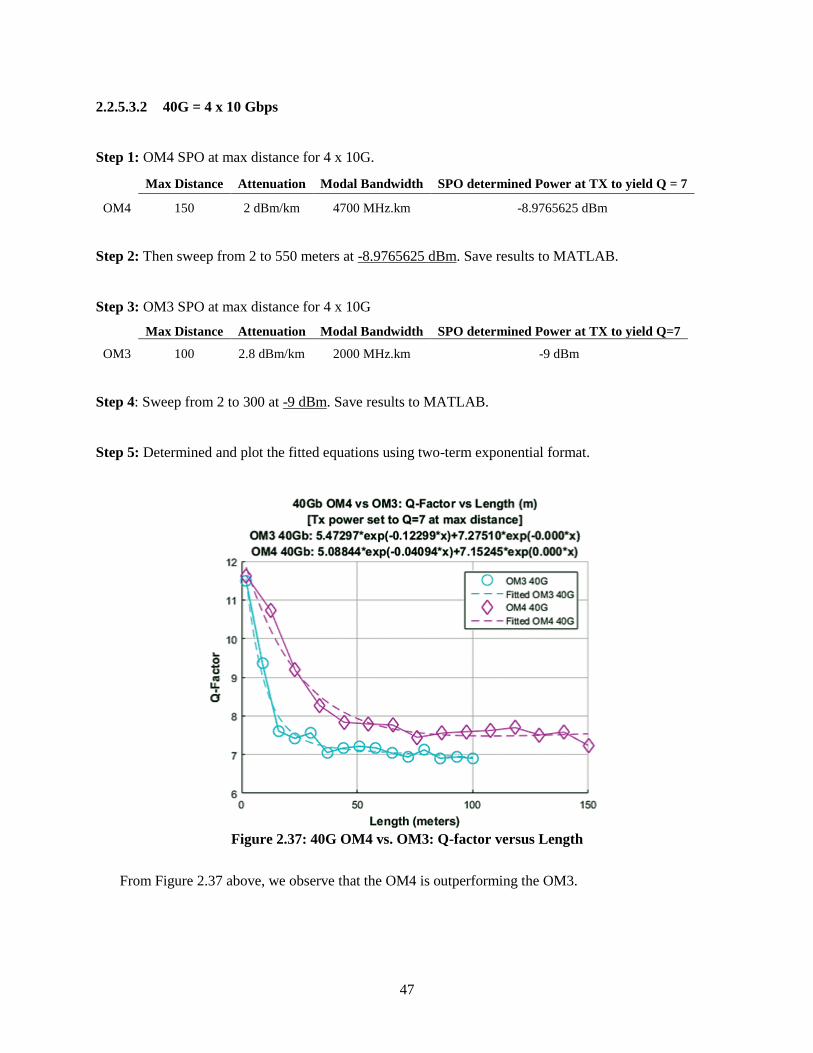
47
2.2.5.3.2 40G = 4 x 10 Gbps
Step 1: OM4 SPO at max distance for 4 x 10G.
Max Distance Attenuation Modal Bandwidth SPO determined Power at TX to yield Q = 7
OM4 150 2 dBm/km 4700 MHz.km -8.9765625 dBm
Step 2: Then sweep from 2 to 550 meters at -8.9765625 dBm. Save results to MATLAB.
Step 3: OM3 SPO at max distance for 4 x 10G
Max Distance Attenuation Modal Bandwidth SPO determined Power at TX to yield Q=7
OM3 100 2.8 dBm/km 2000 MHz.km -9 dBm
Step 4: Sweep from 2 to 300 at -9 dBm. Save results to MATLAB.
Step 5: Determined and plot the fitted equations using two-term exponential format.
Figure 2.37: 40G OM4 vs. OM3: Q-factor versus Length
From Figure 2.37 above, we observe that the OM4 is outperforming the OM3.

48
2.2.5.3.3 100G = 10 x 10 Gbps
Step 1: OM4 SPO at max distance for 10 x 10G.
Max Distance Attenuation Modal Bandwidth SPO determined Power at Tx to yield Q=7
OM4 150 2 dBm/km 4700 MHz.km -5.0 dBm
Step 2: Then sweep from 2 to 150 meters at -5.0 dBm. Save results to MATLAB.
Step 3: OM3 SPO at max distance for 10 x 10G
Max Distance Attenuation Modal Bandwidth SPO determined Power at Tx to yield Q=7
OM3 100 2.8 dBm/km 2000 MHz.km -5.05 dBm
Step 4: Sweep from 2 to 100 at -5.05 dBm. Save results to MATLAB.
Step 5: Determined and plot the fitted equations using two-term exponential format.
Figure 2.38: 100G OM4 vs. OM3: Q-factor versus Length
From Figure 2.38, we observe that the OM4 is outperforming the OM3.
Length (meters)
Q-F
acto
r

49
2.2.5.3.4 Summary of Q-factor vs Length experiments
In Table 2.5 and Table 2.6 are presented the results of the parallel optics experiments.
Table 2.5 OM3: Equations for Q-factor vs. Length (TX Power (dBm) Q = 7 ± .1 at Max Distance) (A) (B) (C) (D)
Power
Fitted
Eqn.
Q=7.0
Power
SPO
Optimized
Q=7 ± .1
Δ Eqn. Based on SPO
(automated)
10G* -20.3269 -20.45 .6% y = 7.37968.*exp(-.000215) (2.5)
40G -8.7757 -9 2.6% y = 5.47297*exp(-0.12299*x)+7.27510*exp(-0.0004*x) (2.6)
100G -5.0241 -5.05 .5%
y = 5.59373292*exp(-0.12927862*x)+7.28378306*exp(-
0.00042308*x) (2.7)
*10G was fitted using 1-term exponential
Table 2.6: OM4: Equations for Q-factor vs. Length (TX Power (dBm) Q = 7 ± .1 at Max Distance) (A) (B) (C) (D)
Power
(dBm)
Fitted
Eqn.
Q=7.0
Power
(dBm)
SPO
Optimized
Q=7 ± .1
Δ Eqn. Based on SPO
(automated)
10G -20.6012 -20.5 .6% y=7.77941*exp(-0.00015*x)+-0.000001*exp(0.021*x) (2.8)
40G -8.767 -8.9765625 2.4% y=5.08844*exp(-0.04094*x)+7.15245*exp(0.00001*x) (2.9)
100G -5.035 -5.0 .5%
y=4.89846*exp(-0.04601*x)+7.22401*exp(0.0001*x)
(2.10)
In Column A, the Power (dBm) fitted values were computed analytically by plotting the sweep of the
power settings in MATLAB, solving for the coefficients of the best-fit of the line using a two-term
exponential equation, and then solving for the power at Q=7 using the equation of the best-fit line. Column
B represents the results from an alternative approach that utilized the Single-Parameter Optimization (SPO)
features of Optisystem, which automatically solved for the optimal power at Q-factor = 7 ± .1. Thus, in
this work are demonstrated two approaches: first is the approach to determine the Q-factor analytically,
and, secondly is the approach for utilizing an automated simulation approach. Column C represents the
delta difference (%) between the two approaches. Column D provides the resulting equation of Q-factor vs
Length, based on the SPO optimization approach. The automated SPO approach was used primarily because
the results are close to the more time-consuming analytical approach. The equations in Column D were the
goal of the experiments, and as such, will be utilized in the system design optimization when evaluating the
trade-offs of optical quality and distance within the design options.

50
2.2.6 Summary of Fiber Optic Technology
In summary, we draw several observations about fiber-optic technology:
1. Optical wavelengths can be focused in glass fibers to span short and long distances;
2. The performance of the optical bandwidth is determined using the measurement for the
Calculated Effective Modal Bandwidth (EMBc);
3. The optical communication design requires a transmitter (TX), channel, and receiver (RX). A
BER analyzer can be attached on the optical receiver to observe and optimize the Q-factor;
4. The quality of the optical signal at the receiver (RX) can be measured with a Q-factor value,
with a Q-factor ≈ 7 representing a Bit Error Rate = 1e-12 which is the minimum value for
guaranteed optical performance. The Q-factor is the Dual of the BER, meaning the optimization
can be either to minimize the BER, or, maximize the Q-factor;
5. Parallel optical channels enables transmission of 10G (1 x 10 Gbps), 40G (4 x 10 Gbps), and
100G (10 x 10 Gbps). The future innovations of optical-networks will rely on parallelism;
6. A target Q-factor can be discovered by sweeping power settings and utilizing a two-term
exponential fitting to determine the coefficients of the best-fit equation. Then using this
equation, it is possible to analytically solve for the target values;
7. Utilizing the OptiSystem simulation Single-Parameter Optimization (SPO) features can rapidly
compute the optimal power through automated simulation; and
8. The fitted equations of Power vs Length in Columns D of Table 2.5 and Table 2.6 above are
generated from theoretical experimentation of OM3 and OM4 multi-mode optical fiber at 10G,
40G, and 100G. These equations are used in the multi-objective fiber-optic system design
optimizations.
In the next section 2.3 is a discussion about data centers.

51
2.3 Data Center
2.3.1 Facilities
Shown in Figure 2.40 below is a representation of the main components of a data center which is useful to
understand the complexity of the infrastructure and will be important in the design of the network and
power requirements to operate the facility:
Figure 2.39: Generic Data Center Facilities Diagram
Source: [47]
The data center facility contains multiple areas of operations, as summarized in Table 2.7 below:
Table 2.7: Summary of Data Center Infrastructure Components
Work Area/Office Spaces
Space Planning/Relocation Area
High-reliable air conditioning system
High head generation countermeasures
Standby-generators
Uninterrupted Power Supply (UPS)
Cable Route/Ducts
Servers/Router Rack
Networking cables
DC Power Supply System
Battery
Commercial Power
Lightning trouble/EMC
Grounding
Security System
7x24 monitoring
Aseismic counter measures
Raised Floors
Overhead raceways
Mobile Generators
Power Receiving Facility
Loading dock facility

52
2.3.2 Segmented Floor Plan
Shown in Figure 2.40 below is a generalized data center fiber-optic network, illustrating the standard’s
based division of three areas: Entrance, Main Distribution, and Horizontal Distribution Area.
Figure 2.40: Generic Representation of a Data Center Floor Plan
Source: [48]
The optical network components for each area are defined in Table 2.8 below:
Table 2.8: Optical Components in a Data Center Floor Plan Section # Name Purpose
Entrance
Facility
1 Splice Frame Organizing optical fiber
2 Optical Raceway Organizing fiber overhead
3 Termination/Splice Fiber Panel Splicing fiber
4 Termination Blocks Terminating connection’s
5 Termination/Splice Fiber Panel Splicing/Terminating
Main
Distribution
Area
(MDA)
6 Optical Distribution Frame Backbone interconnections
7 High-Density Fiber Panel Interconnections of optical cable
8 Storage Area Vertical blade SAN directors
9 Pre-terminated Fiber Optic Cabling Intra-connections
Horizontal
And
Equipment
Distribution
Area
(HDA)
9 Raceway Fiber-Optic multi-mode
10 Angle Left/Right Fiber Panel Cassettes for easy access to ports.
11 Universal Connectivity Platform Enables mix of fiber and cooper cabling
12 Pre-terminated Copper Solutions Factory testing cooper cables
13 Copper Cabling Horizontal cabling
14 Copper Patch Panels Connecting copper
15 Direct Attach Cabled (DAC) Passive and active copper
16 Fiber Patch Panels Patching and splicing

53
2.3.3 Data Center Design Considerations
There are four data center design considerations that are relevant to this thesis work: 1) Tiered Service
Levels, 2) Power Usage Effectiveness (PUE), 3) Power Cost Modeling, and 4) Economics of TOR vs EOR.
2.3.3.1 Tiered Service Levels
In Figure 2.41 below is shown the TIA-942 standard for redundant data center topology.
Figure 2.41: TIA-942 Data Center Infrastructure Redundancy Topology
Source: [15]
Based on the redundant infrastructure levels, Table 2.9 below, data centers are certified into one of four
tiers levels [39]. The tiered service level is increased through redundancy of infrastructure that minimizes
the annual downtime.

54
Table 2.9: Data Center Redundancy Tier Levels
Sources: [70]–[72]
LEVEL Tier 1
Basic Site Tier 2
Redundant Tier 3
Concurrently Maintainable Tier 4
Fault Tolerant
SCOPE
[1] Single path
for power/cooling
distribution
[2] No redundant
components
[1] Single path for
power/cooling
distribution
[2] Redundant
components
[1] Multiple power/ cooling
distribution-- one path active
[2] Redundant components
[3] Concurrently
maintainable
[1] Multiple active
power/cooling
paths
[2] Redundant
components
[3] Fault tolerant
DOWNTIME <28.8 hr/yr < 22.0 hrs/yr < 1.6 hrs/yr <.4 hrs/yr
UPTIME 99.671% 99.749% 99.928% 99.995%
DELIVERY PATHS 1 1 1 Active, 1 Passive 2 Active
REDUNDANCY NO N+1 N+1 S+S, or 2(N+1) COMPARTMENT-
ALIZATION NO NO NO YES
CONCURRENTLY
MAINTAINABLE NO NO YES YES
FAULT TOLERANT
TO WORST EVENTS NO NO NO YES
Due to the financial cost of each escalating tier there are limited Tier 4 facilities. Only two US facilities are
currently Tier IV Gold certified: one in Las Vegas, NV and the second in Olathe, KS [39].
2.3.3.2 Power Usage Effectiveness (PUE)
The most common metric used to express the power efficiency in data centers is defined by [54]:
𝑃𝑈𝐸 = Total power consumed by a datacenter
Power consumed by servers ( 2.11 )
The ratio value of 1.0 is the lowest value that can be attained for Equation 2.11 above. Shown in Figure
2.42 below is an example of the power consumption from a data center power utilization study [54].
Figure 2.42: A Breakdown of Datacenter Energy Overhead Costs
Source: [54, p. 863]
The managers of data centers have to consider the PUE value because it summarizes the costs that drive
the operations of the facility. The study of environmental cooling is a significant area of importance in data
center research. This work takes into consideration the PUE towards the life-cycle cost management.

55
2.3.3.3 Power Cost Modeling
The equations 2.12 - 2.18 below are adapted from [84] for power cost modeling:
Nomenclature:
Rate ≜ Annual cost of money
Facility_Amortize_Periods ≜ Years for amortization
Cost_of_Facility ≜ Total cost of the facility
Infrastructure ≜ Monthly cost of the amortized facility
Num_Servers ≜ Quantity
Cost_Per_Server ≜ Total cost
Server_Amortize_Periods ≜ Years for amortization
Servers ≜ Monthly cost of the amortized servers
Power_Cooling_Infrastructure Percentage ≜ Power cooling of infrastructure as percentage
Power_Cooling_Infrastructure ≜ Power cooling of infrastructure as dollars
Mega_WattsCritical_Load ≜ Critical load for the facility
Average_Power_Usage ≜ Average power usage
PUE ≜ Power usage effectiveness
PowerCost_kwh ≜ Cost per kilowatt hour
Power ≜ Monthly power costs
Other_Infrastructure ≜ Monthly cost of other infrastructure
Full_Burdened_Power ≜ Power for cooling and power for systems
Total_Cost ≜ Total cost of power
Infrastructure = payper (Rate
12, Facility_Amortize_Periods ∗ 12, Cost_of_Facility, 0,0) ( 2.12 )
Servers = payper (Rate
12, Server_Amoritze_Periods ∗ 12, Num_Servers ∗ Cost_Per_Server, 0,0) ( 2.13 )
Power_Cooling_Infrastructure = (Infrastructure ∗ Power_Cooling_Infrastructure_Percentage) ( 2.14 )
Power = (Mega_WattsCritical_Load ∗Average_Power_Usage
1000∗ PUE ∗ PowerCost_kwh ∗ 24 ∗
365
12) ( 2.15 )
Other_Infrastructure = (Infrastructure − Power_Cooling_Infrastructure) ( 2.16 )
Full_Burdened_Power = (Power_Cooling_Infrastructure + Power) ( 2.17 )
Total_Cost = (Infrastructure + Servers + Power) ( 2.18 )
The formulation of these equations is adapted into the MATLAB code (see Appendix 5.1).

56
2.3.3.4 Economic comparison of TOR vs. EOR
An important aspect of each data center cabinet is the switching equipment within the rack, of which there
are two dominant approaches: Top of Rack (TOR) and End of Row (EOR). To understand the impact of
choosing TOR versus EOR on life-cycle costs, an economic study was developed by [76] comparing a 144-
Server configuration (see Figure 2.51 and Figure 2.53 below), as summarized in Table 2.10 below:
Table 2.10: TOR vs. EOR: Economic Comparison of Low and High Density (144 Server Cabinets)
Source: [76]
CASE A CASE B
Low-Density, 144 Server Cabinets
14 Servers Per Cabinet High-Density, 144 Server Cabinets
40 Servers Per Cabinet
Material, Power
& Maintenance
ToR
(SFP+)
EOR
(10BASE-1)
Material, Power
& Maintenance
ToR
(SFP+)
EOR
(10BASE-1)
Material Cost $ 11.78M $ 8.64M Material Cost $ 26.39M $ 21.6M
Annual Maintenance Cost $ 1.66M $ 1.28M Annual Maintenance Cost $ 3.37M $ 2.74M
Annual Energy Cost $ .1M $ .04M Annual Energy Cost $ .18M $.11M
Total Cabling
(including in Material Cost) $ 1.22M $ .70M
Total Cabling
(including in Material Cost) $ 5.12M $ 2.08M
Total Cost of Ownership $ 13.5M $9.97M Total Cost of Ownership $ 35.06M $24.44M
The example provides a good illustration of how two different architectures can dramatically impact
the density and the total costs. In the Low Density Case A, the EOR Total Cost of Ownership (TCO) was
$9.97M; while in the High Density Case B, the EOR TCO increased to $24.4M. Similarly, the TOR
configuration increased and remained larger than EOR in both cases. In considering the different
architecture types, the problem becomes dramatically more complex and trade-offs between infrastructure
design, cost, and flexibility begin to present options to the data center decision manager.
2.3.4 Summary of Data Center
In summary, we can draw the following observations about data centers:
1. The topology of data center facilities are segmented into standards-based zones.
2. The design of data centers needs to consider: Redundancy tiers levels of key infrastructure,
Power Usage Effectiveness, Power cost modeling; and Economics of using Top of Rack versus
End of Row networking configurations.
3. The Total Cost needs to consider both the long-term amortized facility costs and the monthly
power costs. Though the initial facility cost will be amortized over 15 to 20 years, and the
server/network equipment over 3 to 5 years, the incurred power cost incurred is a monthly rate,
and may experience fluctuations due to changes in kilowatt per hour market rates.
In the next section, is the discussion on the approach to considering Systems Analysis.

57
2.4 Systems Analysis
In this work, the goal is evaluate a system, specifically, a fiber-optic system within data centers. To perform
this systems-based evaluation, we need to understand: how the influences that drive ‘functionality’ of the
architecture translate to the ‘form’ of the system. In the following sections is a review, and synthesis, of the
corresponding literature.
2.4.1 Overview
Shown in Figure 2.43 below is the mapping of what are considered upstream influences that map to systems
architecture. In this work, I consider the influences within the context of an analytical and heuristic
approach, and therefore, rely mostly on the translation of the Beneficiary/Customer Needs to Goals and the
optimization of the Technology, as highlighted in red.
Figure 2.43: Mapping Function to Form
Source: [69]
To develop a holistic view of a system, I propose in this thesis, that we can employ a set of systems
analysis tools in a sequence as shown in Figure 2.44 below as an approach to build-up the systems
knowledge in a step-wise and layered manner:
Figure 2.44: Systems Analysis Process (Topology>Hierarchy>OPM)
Shown in Figure 2.44 above, is a proposed sequence for developing an isometric systems perspective,
defined in the following step-wise manner:
Define the Topological relationships of form and function for the components. [73]
Specify the Hierarchical relationships. [73]
Model the Objects and processes with Object-Process Methodology (OPM). [42]

58
2.4.2 Topology
The three main elements of a topological representations are illustrated in Figure 2.45: (1) The components
of the system, represented by {A,B,C,D,E}, (2) the connection types between the components (e.g.,
physical, logical, etc.), and (3) the boundary of the relationship. [69], [73]
Figure 2.45: Generic Format for a Topological Representation
Utilizing the topological representations, shown in Figure 2.22 and Figure 2.40 above, is important for
evaluating the physical relationships between the components. [46]
In this work, I apply the analysis towards evaluating the TIA-942 Star Topology, Figure 2.46 below,
for collocation data center fiber-optic networks.
Figure 2.46: TIA-942 Star Topology
Source: [38]
A B
EC
D
[2] Physical Connection
[3] Sub-system boundary
[1] System Component

59
2.4.3 Hierarchy
The generic format for representing a hierarchal structure, as in Figure 2.47 below, identifies the
dependences for a vertically integrated system. The use of defining hierarchical relationships in the design
of data centers and fiber-optic networks is essential to consider the entire system and how data will flow.
Figure 2.47: A Generalized Hierarchical Decomposition
Shown in Figure 2.48 below is an example of a hierarchical representation of one example for a data center
architecture which is divided into 7 layers: Core, Aggregation, Access, Server Farms, Edge, Core, and
Storage/Tape/Media Farms. The cross-connections create horizontal integration of Server Clusters.
Figure 2.48: Hierarchical Architecture of a Multi-tier Data Center
Source: Adapted from Cisco Systems, Inc.
One of the most dominant hierarchical structure currently used is referred to as the FatTree [54], referring
to the tree, and root structure design.
As shown in Figure 2.49 below, the floor layout of a data center is arranged in a grid configuration,
with rows of rack (aka, cabinets), configured in columns, and separated by walking ailseways. In Figure
2.49 below is shown two alternatives of the configuration, and different power requirements configurations.
This grid configuration is an industry format for physical configuration of the rack.

60
Figure 2.49: Rack Layout and Power Requirements
Source: [71]
The grid configuration for the racks is an important characteristic for the network design because it relates
to the type of network hierarchical architecture that will exist in the data center to interconnect the cabinets.
2.4.3.1 Top of Rack (TOR)
The Top of the Rack (TOR) configuration shown in Figure 2.50 below utilizes one switch, typically placed
at the top of the cabinet, which is connected via a fiber-optic uplink to the Aggregation Layer Switch.
Figure 2.50: TOR Configuration
Source: [75]
In a top-down view of a data center floor plan shown in Figure 2.51 below, we can observe that the
complexity and manageability quickly escalates to include cost of installation costs, maintainability,
operating cost, and utilization. In the example of Figure 2.51, each row represents 14 Server Cabinets with
redundant fiber (yellow and green) running from core to EOR distribution points and from there to the TOR
Access Switches in each server cabinet. Point-to-Point cabling is confined to within the cabinet from TOR
Switches to servers [76].
Fiber Uplinks
Patch Panel Top of Rack
Switches
Cooper
Patch Cables
Servers Aggregation
Layer Switch
Rack – Rack Interconnect

61
Figure 2.51: 144-Cabinet TOR Configuration in a Data Center
Source: [76]
In Table 2.11 below is summarized several of the Pros and Cons of using the TOR configuration.
Notably, this hierarchy is easy to upgrade and typically known for lower cost of cabling, but higher
investment in the Aggregation Layer Switch.
Table 2.11: Pros and Cons of Top of Rack (TOR)
Source: [74]
Pros Cons
1. Per rack architecture which is easy to
upgrade.
2. Problem of one switch affects lower
number of servers.
3. Most of the wiring is in rack.
4. Cleaner cable management, lower costs of
cables (because of length, although more is
needed to aggregation level).
1. More switches to manage.
2. Worse scalability (number of STP
instances, STP scalability, connections
to aggregation level).
3. Increases costs of hardware, because of
number of switches.
4. Single point of failure with the
Aggregation Layer Switch to the entire
row.
2.4.3.2 End of Rack (EOR)
The End of Row (EOR) configuration shown in Figure 2.52 below utilizes a patch panel, typically placed
at the top of the cabinet, which is then interconnected to the patch panel at the End of the Row cabinet
where the End of Row Switch will reside.
Figure 2.52: EOR Configuration
Source: [75]
Patch Panel
Rack – Rack Interconnect
Cooper
Patch Cable
Servers Servers End of Row
Switch
Patch
Panel

62
In a top-down view of a data center floor plan shown in Figure 2.53 below, each row represents 14 Server
Cabinets with redundant fiber (yellow and green) running from core to EOR access switches and redundant
Category 6a 10GBASE-T Cooper Cabling (Red and Blue) from EOR to each Server Cabinet [76].
Figure 2.53: 144-Cabinet EOR Configuration in a Data Center
Source: [76]
In Table 2.12 below is presented a summary for consideration about the EOR approach to data center.
Table 2.12: Pros and Cons of End of Rack (EOR)
Source: [58]
Pros Cons
1. Lower number of switches (less expensive
hardware).
2. Better manageability of switches (lower
costs to manage them).
3. Fewer ports required to distribution layer.
4. Less STP instances, better scalability on
logical level.
5. Usually higher availability for servers.
6. Easy to replace module or line card (In
TOR, usually whole switch must be
replaced).
1. Challenges in cable management and
installation, more expensive because of
lengths--- much longer wiring from all the
racks.
2. Worse scalability in the future, when
switching to higher speeds. Worse
scalability on physical level.
3. Challenges in replace or upgrade of
switches – multiple racks can be affected
(doesn’t has to be disadvantage, if
redundancy and high availability is well
designed).
4. Careful planning on high availability and
redundancy.

63
2.4.4 Object-Process Methodology (OPM) and Diagrams (OPD)
As defined by [77, p. 104], “Object-Process Methodology (OPM) is a language that describes function in a
general approach that can span disciplines, and simultaneously provide precision the semantics and
representations. OPM is a powerful way that captures exogenous influences, internal functions, functional
attributes, subsystems, design variables, and the role of actors in the system.”
Figure 2.54: Generic Format for an OPD Representation
Reference: [42], [73], [69]
As represented in Figure 2.55 below, the OPD method is especially useful in this thesis because it helped
the author to conceptualize and map the multi-layered processes (function) and objects (forms) of a complex
data center system and define the boundaries of the system and scope of this thesis.
.

64
Figure 2.55: OPD of a Data Center representing Process Projected onto Form
Reference: [42], [73], [69]
Da
ta C
en
ter
Wh
ole
Sy
ste
m B
ou
nd
ary
Co
nstr
uctin
g
Co
nn
ectin
g
Sto
rin
g
De
cis
ion
Ma
na
ge
r
Use
r
Su
pp
ort
ing
Ob
jec
ts a
nd
Inte
rfa
ce
s
Su
pp
ort
ing
Pro
ce
ss
es
Co
olin
g
Po
we
rin
g
Arc
hiv
ing
Co
mm
un
ica
tin
g
Co
nta
inin
g
Va
lue
Pro
ce
ss
Ins
tru
me
nts
Co
mp
utin
g
Se
cu
rin
g
Ele
ctr
ifyin
g
Co
pp
er
Ca
ble
s
Pro
ce
sso
rs
Mu
lti-M
od
e
Fib
er
Ne
two
rkin
g
Po
rts
Ch
ille
rs
Re
so
urc
es
Sin
gle
-Mo
de
Fib
er
Sto
rag
e D
rive
s
Th
es
is F
oc
us
Bo
un
da
ry
Hyd
ro-E
lectr
ic
Nu
cle
ar
So
lar
Ga
sW
ind
Grid
La
nd
Pla
ns
Fu
nd
ing
Ma
teria
lsC
on
tra
cto
rs
10
0 M
bp
s1
Gb
ps
10
Gb
ps
40
Gb
ps
10
0 G
bp
s4
00
Gb
ps
9/1
25
OM
1
50/1
25
OM
2
50/1
25
OM
3
50/1
25
OM
4
62
.5/1
25
OM
2
CA
T.5
CA
T.5
e
CA
T.6
CA
T.7
CP
UG
PU
SS
DS
AT
AS
CS
I
Lic
en
se
s
Wa
ter
Po
we
r
Co
ol W
ate
rA
irO
il
Co
olin
g
Ag
en
t L
ink
Instr
um
en
t L
ink
Effe
ct L
ink
Pro
ce
ss
Instr
um
en
t
Sp
ecia
lize
s to
LE
GE
ND
Ca
bin
ets
Se
rve
rs
Ca
blin
g
Inte
rne
t
Sw
itch
es
Ro
ute
rs
Bu
ildin
g
Air
Co
nd
itio
ne
rs
UP
S
Ge
ne
rato
rs
Po
we
r
Lin
es

65
From the Figure 2.55 above, the OPL specification is generated, Table 2.13 below, which helps define the
multi-layered architecture of process and objects of the data center fiber-optic network system.
Table 2.13: OPL Specification for a Data Center
Reference: (Dori 2002) [42]. Generated using OPCAT II. Generators is physical.
Building is physical.
Power Lines is physical.
Air Conditioners is physical.
Cabinets is physical.
Cabinets handles Storing.
Servers is physical.
Servers handles Computing.
Switches is physical.
Switches handles Connecting.
Cabling is physical.
Cabling handles Connecting.
Single-Mode Fiber is physical.
Multi-mode Fiber is physical.
UPS is physical.
50/125 MM OM2 is physical.
50/125 MM OM3 is physical.
50/125 MM OM4 is physical.
Storage Drives is physical.
Processors is physical.
Copper is physical.
Routers is physical.
Routers handles Connecting.
Networking Ports is physical.
Utility is physical.
Internet is physical.
Internet handles Connecting.
100 Mbps is physical.
100 Mbps is a Networking Ports.
1 Gbps is physical.
1 Gbps is a Networking Ports.
10 Gbps is physical.
10 Gbps is a Networking Ports.
40 Gbps is physical.
40 Gbps is a Networking Ports.
100 Gbps is physical.
100 Gbps is a Networking Ports.
9/125 OM1 is physical.
9/125 OM1 is a Single-Mode Fiber.
62.5/125 MM is a Multi-mode Fiber.
CAT.5 is physical.
CAT.5 is a Copper.
CAT.6A is physical.
CAT.6A is a Copper.
CAT.7 is physical.
CAT.7 is a Copper.
CAT.5e is physical.
CAT.5e is a Copper.
SSD is physical.
SSD is a Storage Drives.
SCSI is physical.
SCSI is a Storage Drives.
SATA is physical.
SATA is a Storage Drives.
CPU is physical.
CPU is a Processors.
GPU is physical.
GPU is a Processors.
NPU is physical.
NPU is a Processors.
Hydro-Electric is physical.
Hydro-Electric is an Utility.
Solar is physical.
Solar is an Utility.
Nuclear is physical.
Nuclear is an Utility.
Gas is physical.
Gas is an Utility.
Wind is physical.
Wind is an Utility.
Grid is physical.
Grid is an Utility.
Land is a Resources.
Funding is a Resources.
Licenses is a Resources.
Plans is a Resources.
Materials is a Resources.
Contractors is a Resources.
400 Gbps is a Networking Ports.
Electrifying is physical.
Electrifying requires Utility.
Electrifying affects Building, Servers,
Switches, Routers, and Air Conditioners.
Electrifying yields UPS, Generators, and
Power Lines.
Containing is physical.
Containing requires Building.
Communicating is physical.
Communicating requires Servers, Internet,
Routers, Switches, and Cabling.
Archiving is physical.
Archiving requires Servers.
Securing is physical.
Securing requires Building and Cabinets.
Storing is physical.
Storing requires Servers and Storage Drives.
Connecting requires Networking Ports,
Copper, Multi-mode Fiber, and Single-mode
Fiber.
Computing is physical.
Computing requires Processors.
Powering is physical.
Powering requires Generators, Power Lines,
and UPS.
Constructing is physical.
Constructing requires Utility and Resources.
Constructing yields Building.
Cooling is physical.
Cooling occurs if Building is in existent.
Cooling requires Air Conditioners.
With the OPL, we can gain an understanding of the multi-layered processes and forms of the system.
2.4.5 Summary on Systems Analysis
The implementation of the system’s thinking based approaches has enabled a methodology to deconstruct
a complex system and define the interacting components. Through the SA analysis, we can develop a focus
on the primary aspects of interest and study the relationship of the form and function of the system. The
unified language of OPM/OPD allows us to thoroughly represent the system and the boundaries of focus.
Based on the research between TOR vs EOR, the model in this work is based only on TOR configurations.

66
2.5 MOGA: Multi-Objective Optimization with Genetic Algorithms
In this work, I aim to consider an existing optimization approach and then develop a holistic framework
that will consider the systematic definition of the design vector inputs into a model, and then empower a
decision manager with an automated analysis of the trade-offs between life-cycle cost, system user capacity,
and optical transmission performance (Q-factor).
In the following Sections 2.5.1 - 2.5.7 is presented a discussion on the heuristic optimization approach
of Multi-objective Optimization with Genetic Algorithms (MOGA) within the Multidisciplinary System
Design Optimization (MSDO) framework [4].
2.5.1 MSDO: Multi-Disciplinary System Design Optimization Framework
Shown in Figure 2.56 below is the MSDO Framework [4], which is composed of five elements: Design
Vector of inputs, Simulation Model that considers inputs and outputs of the specific disciplines of the
research, an Objective Vector of outputs, a coupling stage gate with various Output Evaluations methods,
Optimization Algorithms, and another coupling that includes the Tradespace Exploration.
Figure 2.56: Multidisciplinary System Design Optimization Framework
Source: [4]

67
The two main components of the framework are the (1) Simulation Model, which evaluates for optimal
designs, and the (2) Optimization Algorithms, which define the movement pattern and search approach
through the design space.
To execute the process, a general process is proposed [4]:
Step 1: Define overall system requirements.
Step 2: Define design vector x, objective J and constraints.
Step 3: System decomposition into modules.
Step 4: Modeling of physics via governing equations at the module level.
Step 5: Model integration into an overall system simulation.
Step 6: Benchmarking of model with respect to a known system from past experience, if available.
Step 7: Design space exploration to find sensitive and important design variables xi.
Step 8: Formal optimization to find min J(x).
Step 9: Post-optimality analysis to explore sensitivity and tradeoffs: sensitivity analysis,
approximation methods, isoperformance, including uncertainty.
However, MSDO is a highly interactive practice, and in true practice, Steps 1 – 8 may not occur linearly,
in which a branch in the process may occur. There may be an error that precipitates a solution that is
unreasonable, or a feasible solution will not be found. In either case, the interaction of the research is
required to make adjustments and use practical logic to adjust the research direction.
Lastly, an important aspect of this framework is to consider trade-offs for increasing difficulty. The
plots shown in Figure 2.57 below represent how we should consider the level of effort for achieving high
accuracy versus fidelity, and the breadth of the analysis versus the depth.
Figure 2.57: Considering Challenges of Increasing Computational Difficulty
Source:[4] (adapted from Giesing and Barthelemy 1998)
The role of the research architect is to find the proper balance for the analysis at hand.

68
2.5.2 Design Variables
The design space is composed of a vector 𝐱 of 𝑛 variables that forms the design space for exploration in
which the values for the entries of x are changed in a rational manner towards a desired effect; the variables,
which can have different units and types, are the controls by which the designer sets the parameters for
exploring the trade-space [4].
In a fiber-optic network, a design vector can be represented as:
𝐱 =
[ 𝑥1
𝑥2
𝑥3
𝑥4
𝑥𝑖
⋮𝑥𝑛]
=
[
core sizetransmit power
lengthfrequency
attentuationbit rate
modal bandwidththermal power density
Rx Sensitivitytarget Q-factor
cost ]
( 2.19 )
The values for 𝑥𝑖 can be expressed as various types [85]:
Table 2.14: Notation for Number Types Type Name Example
Real 𝑥𝑖 ∈ ℝ -10.1, 3.1, 5.8, 8
Integer 𝑥𝑖 ∈ ℤ -3, 0, 125
Binary 𝑥𝑖 ∈ {0,1} 11111011111
Boolean 𝑥𝑖 ∈ 𝔹 false (0), true (1)
Complex 𝑥𝑖 ∈ ℂ 4 + 8.2√−1
2.5.3 Objective Functions
The process for performing a global optimization begins with the definition of the problem [6]:
𝑚𝑖𝑛𝑥
𝐽(𝑥) ( 2.20 )
subject to
𝑔(𝑥) ≤ 0 ( 2.21 )
ℎ(𝑥) = 0 ( 2.22 )
𝑥𝐿𝐵 ≤ 𝑥 ≤ 𝑥𝑈𝐵 ( 2.23 )
The objective function 𝐽(𝑥) is represented by Equation 2.20. In Equation 2.21 is defined the inequality
constraint 𝑔(𝑥) and the equality constraint ℎ(𝑥) by Equation 2.22. The lower bound 𝑥𝐿𝐵 and the upper-
bound 𝑥𝑈𝐵 for 𝑥 are defined by Equation 2.23.
Shown in Figure 2.58 below is a common example for discussing global maximum and minimum using
the multivariate MATLAB “Peaks” objective function, Equation 2.24, [88]:
z = 3*(1-x).^2.*exp(-(x.^2) - (y+1).^2) ...
- 10*(x/5 - x.^3 - y.^5).*exp(-x.^2-y.^2) ...
- 1/3*exp(-(x+1).^2 - y.^2)
( 2.24 )

69
The global minimum is discovered by minimizing z, and the global maximum can be discovered by
minimizing (-1).*z. The solution is:
Global Min = [X1 X2 Z] = [0.2328 −1.6135 −6.5490] Global Max = [X1 X2 Z] = [−0.0127 1.5827 8.1061]
( 2.25 )
Figure 2.58: Global Max and Global Min of the Peaks Objective Function
While the Peaks example is a simple one, and can be solved fairly quickly (i.e., seconds) with modern
day software, the complexity of more sophisticated problems becomes computationally too expensive,
especially when solving for multiple objective functions simultaneously. Therein lies the need for
developing efficient algorithms that can facilitate the discovery of the trade-space characteristics.
2.5.4 Multi-Objective Optimization
As proposed in Section 1.1 Figure 1.1 above: in managing real systems we must frequently consider
multiple business objectives. The objective is a vector 𝐉 of z system responses which we aim to maximize,
or minimize, and defined as [4]:
𝐉 =
[
𝐽1
𝐽2
𝐽i
⋮
𝐽𝑍
]
=
[
cost ($)
noise (dB)
capacity (users)
⋮
power (W)
]
( 2.26 )
In Equation 2.26 is presented an example vector 𝐉 of system-level metrics that are used when considering
fiber-optics network design.

70
The problem formulation is then updated to reflect the multi-objective approach, with vector notation:
𝑚𝑖𝑛𝐱
𝐉(𝐱) ( 2.27 )
subject to
𝐠(𝐱) ≤ 0 ( 2.28 )
𝐡(𝐱) = 0 ( 2.29 )
𝑥𝑖,𝐿𝐵 ≤ 𝑥𝑖 ≤ 𝑥𝑖,𝑈𝐵
𝑖 = 1,… , 𝑛 ( 2.30 )
𝐉 = [𝐽1(𝐱) ⋯ 𝐽𝑧(𝐱)]𝑻 ( 2.31 )
𝐱 = [𝑥1 ⋯ 𝑥𝑖 ⋯ 𝑥𝑛]𝑻 ( 2.32 )
𝐠 = [𝑔1(𝐱) ⋯ 𝑔𝑚1(𝐱)]𝑻 ( 2.33 )
𝐡 = [ℎ1(𝐱) ⋯ ℎ𝑚2(𝐱)]𝑻 ( 2.34 )
The Equations 2.27 - 2.34 form the foundation for the multi-objective optimization utilized in this work.
2.5.5 Multi-Objective Heuristics with Genetic Algorithms
The motivation for heuristic optimization techniques is to develop a means for analytical computation to:
1) address local optima getting trapped and resulting in the global minimum not being accurately discovered
and 2) allow continuous and discrete, 𝑥𝑖 ∉ ℝ, design variables [89]. By invoking a rules-based randomness
into the techniques, heuristics allow for better discovery of the global optimums in situations which might
otherwise not be found with the classical (i.e., gradient/calculus-based hill climbing) techniques.
Throughout time, scientists and engineers have looked to nature for inspiration in many aspects of
product development, with a prime example in the field of Aeronautics and Aviation is the airplane— a by-
product of bird wing designs. Similarly, in the field of global optimization, an evolutionary algorithm, called
Genetic Algorithms (GA), was developed by [94], in which biological abstractions are applied to a new
paradigm: “population-based metaheuristics optimizations.” [6]
In the spirit of following Darwin’s theory, [5] defined an algorithm, which utilizes the concept of
survival of the fittest in natural selection by considering five parameters: 1) Variation, 2) Competition, 3)
Offspring, 4) Genetics, and 5) Natural Selection [95]. The variation introduces the mutation, competition
considers scarcity of resources, offspring are the result of fertile parents, genetics are the traits which are
passed-on between generations, and natural selection is the process by which only those with the most
effective traits survive. The premise of the GA is to represent a solution in binary format as a chromosome,
and then mutate and crossover the alleles to re-evaluate towards convergence of the fittest solution.
Figure 2.59: Mapping Chromosomes to Binary
Source: [89]

71
By adapting the principles of genetics and natural selection into optimization methods, we are able to
develop computational approaches, Figure 2.60 below, that iteratively solve for optimal solutions. [96]
Figure 2.60: Procedure for Genetic Algorithm
Adapted from: [6], [96]
2.5.5.1 Encoding and Decoding Chromosomes
The process for encoding refers to the conversion of a string (i.e., chromosome) into binary format. In
MATLAB, the ‘dec2bin’, ‘encode’, and ‘decode’ functions may be used. Alternatively, the MATLAB
Optimization Toolbox will perform this process with the built-in procedures when used with ‘gaoptimset’.
Below are examples of encoding, Equation 2.35, and decoding, Equation 2.36, for the number: 2016.
ENCODING EXAMPLE: 2016 to binary
Divide by 2 Value Remainder Binary
1/2 0 R1 > 1
3/2 1 R1 > 1
7/2 3 R1 > 1
15/2 7 R1 > 1
31/2 15 R1 > 1
63/2 31 R1 > 1
126/2 63 R0 > 0
252/2 126 R0 > 0
504/2 252 R0 > 0
1008/2 504 R0 > 0
2016/2 1008 R0 > 0
2016 in binary is 11111100000
Check using MATLAB:
≫ dec2bin(2016) = 11111100000
( 2.35 )

72
The decoding is the conversion from the binary number to the decimal number. DECODING EXAMPLE: 11111100000 to decimal
Binary 1 1 1 1 1 1 0 0 0 0 0
Base2 10 9 8 7 6 5 4 3 2 1 0
≫ decode = 𝟏 ∗ 2.𝟏𝟎+ 𝟏 ∗ 2.𝟗+ 𝟏 ∗ 2.𝟖+ 𝟏 ∗ 2.𝟕+ 𝟏 ∗ 2.𝟔+ 𝟏 ∗ 2.𝟓+ 𝟎 ∗ 2.𝟒+ 𝟎 ∗ 2.𝟑
+ 𝟎 ∗ 2. ^𝟐 + 𝟎 ∗ 2. ^𝟏 + 𝟎 ∗ 2. ^𝟎
≫ decode = 2016
( 2.36 )
2.5.5.2 Initialize Population
The start of the algorithm requires an initial starting point, which requires the definition of the encoding
parameters, size of the population, both in quantity and bits for encoding. These design decisions have a
strong influence on algorithm efficiency, and therefore, careful considered is need to set these values.
2.5.5.3 Fitness
The assignment of fitness is performed on the objective value, with stronger bias towards more fitness, but
ensuring diversity in the population. There are numerous methods for selecting the fitness level criteria,
such a Ranking, Proportionality, Top levels, and Roulette Wheel, to name a few. With each iteration, only
a select subset of parents will be selected to continue to create off-spring.
2.5.5.4 Cross-over
At a cross-over point in the chromosome, binary values of the two parents are swapped to create off-spring.
PARENT 1 1 1 1 1 1 1 0 0 0 0 0
PARENT 2 1 1 1 0 1 1 1 1 1 0 0
OFFSPRING 1 1 1 1 1 1 1 1 1 1 0 0
OFFSPRING 2 1 1 1 0 1 1 0 0 0 0 0
Figure 2.61: Genetic Algorithm Cross-Over
The OFFSPRING 1 contains the first half of the PARENT 1 and second half of PARENT 2. The
OFFSPRING 2 contain the first half of the PARENT 2 and second half of PARENT 1. Next, based on an
insertion strategy, the two OFFSPRING will then return into the algorithm and be evaluated.

73
2.5.5.5 Mutation
Mutation can be introduced by then flipping one of the binary values, using a random probability.
OFFSPRING1 1 1 1 1 1 1 1 1 1 0 0
MUTATED_OFFSPRING1 1 1 1 1 1 1 1 1 1 0 1
Figure 2.62: Genetic Algorithm Mutation
2.5.5.6 Elitistism and Insertion
A small percentage of the fittest individual will be guaranteed survival to the next iteration without any
change in the current iteration. Other strategies for insertion include “Hall of Fame”, in which past
individuals are remembered and not used for the progeny.
2.5.6 Pareto Front
When considering multiple objective functions, it is useful to understand that more than one optimal
solution may be achieved, which is referred to as: Pareto Optimal Solutions. To understand the trade-offs
between the competing objective functions, for example, Obj1 and Obj2 in Figure 2.63 below, we generate
a plot of the dominated and non-dominated solutions, and then look for the line at the edge, called a Parteo
Frontier. This Pareto Front represents the optimal solutions “… for which any improvement in one objective
will result in the worsening of at least one other objective.” [6, p. 125]
Figure 2.63: Example of a Pareto Frontier
Adapted from [4] Leo Satellite Constellation Project
With an understanding of the Pareto front, we are able to consider the trade-offs between the objective
functions and select the point along the Pareto to determine the corresponding design variables that were
used to yield that non-dominated solution.
DOMINATED
NON-DOMINATED

74
2.5.7 Summary of MOGA
In summary, we draw the following observations about multi-objective optimization with genetic
algorithms:
1. We can look to nature for bio-inspired approaches to optimize system designs;
2. Charles Darwin’s theory of evolution and natural selection, and Gregor Mendel’s discoveries of
genetic inheritance have been applied to optimization theory, yielding an evolutionary
algorithm to facilitate discovery of optimal solutions;
3. Encoding solutions into binary format allows for selecting cross-over, mutation, and insertion
strategies for iterative evaluation;
4. Achieving more than one optimal solution leads to a tradespace evaluation of solutions;
5. In evaluating the tradespace, the solutions that are non-inferior (aka, non-dominated) will be
represented along the edge of solution space, which is referred to as the Pareto frontier;
6. A Nadir is the idealized worst solution, and the Utopia is the idealized best solution; and
7. Visualizing the Pareto frontier allows a decision maker to evaluate trade-offs, and thereby
improve the decision making process for evaluating system design.
In the next section, is a discussion of the approach to considering parallel computing with CPU and GPU.

75
2.6 Parallel Computing with CPU and GPU
The growth of computing resources as demonstrated by Moore’s law [109] has brought substantial
computing resources the user’s desktop that once were limited to organizations with large financial
resources. Enabling clusters of parallel processors has become a mainstay resource. The latest trend is
shifting computational resources to harness the multi-core capabilities of Graphic Processing Units (GPU)
to coincide with CPU’s in parallel processing toolboxes. These parallel computing resources enable rapid
computational analysis, which are implemented into the framework of this work.
2.6.1 Vectorized of Functions on the CPU
To improve the performance of the computations within MATLAB, it is best to develop the code to use
arrays or matrices because MATLAB was engineered to perform optimally when using matrix-based (i.e.,
linear algebra) calculations. To help the researcher develop the optimal code towards functions that
‘vectorize’ the data, MATLAB provides built-in methods that offer sophisticated approaches to perform
the vectorization of a function, which include ‘meshgrids’ and ‘bsxfun’. To understand the benefit of coding
one ‘vectorize’ format method over the other, a benchmarking experiment was setup to compare the cputime
for execution of a vectorization, using three approaches: FORLOOP, MESHGRIDS, and BSXFUN.
2.6.2 Analysis of Vectorization on Computation Time with CPU
Figure 2.64: Impact of Three Vectorization Approaches on CPU Computation Time
From Figure 2.64 above, we can draw an observation that for small matrix sizes (<5), the approaches are
relatively equal in time performance. For the range between ~4 to ~35, the ‘for loop’ should be avoided,
and the ‘mesh’ performs best. For the matrix sizes greater than ~36, the ‘bsxfun’ provided the best response.
Understanding the scope of the matrix size for the associated MATLAB code will help the researcher
balance between the exertion of developing sophisticated coding and the performance gain. For small
matrices and quick prototyping the ‘for loop’ is adequate; mid-size matrices, ‘mesh’ works well; and for
the large matrices, the ‘bsxfun’ is best.

76
To increase the speed of a Genetic Algorithm optimization, the fitness function needs to be programmed
in a ‘vectorize’ format [105]. There are several methods to vectorize a function, provided by the following
adopted example [104]:
𝑓(𝑥1, 𝑥2) = 𝑥12 − 2𝑥1 𝑥2 + 6𝑥1 + 𝑥2 − 6𝑥1 ( 2.37 )
Step 1: Vectorized Format of Function:
𝑧 = 𝑥(: ,1). ^2 − 2 ∗ 𝑥(: ,1).∗ 𝑥(: ,2) + 6 ∗ 𝑥(: ,1) + 𝑥(: ,2). ^2 − 6 ∗ 𝑥(: ,2) ( 2.38 )
The colon in the first entry of 𝑥 indicates all the rows of 𝑥, so that 𝑥(: ,1) is a vector.
The .^ and .* operators perform elementwise operations on the vectors.
Step 2: Set the gaoptimset options 'Vectorize’ to on:
options = gaoptimset(options,'Vectorize','on');
To understand the computational benefit of the Vectorized fitness on the GA, a benchmark comparison of
a genetic algorithm [91] is performed, with a starting point of the MATLAB provided demo file:
gaoptionsdemo.m [92]. Two versions of the file were branched and the output of the GA solver were
compared.
Step 0) Modify three options to saturate the computer system
opts = gaoptimset(opts,'PopulationSize',100); Population = rand(10,2); opts = gaoptimset(opts,'Generations',500,'StallGenLimit', 100);
Step 1A) gaoptionsdemo_Vectorize_OFF.m
%% File with the Vectorize OFF by commenting off the option %opts=gaoptimset('Vectorize','on');
Step 1B) gaoptionsdemo_Vectorize_ON.m
%% Vectorize is enabled ON Opts = gaoptimset('Vectorize','on');
Presented in Table 2.15 below is shown the results of the two simulations. We observe that the
‘Vectorize’ option reduces the number of generations and evaluations, while yielding a better result of the
objective function, all within a faster speed. For a single objective function, the performance benefit of
enabling the ‘Vectorize’ option provides substantial benefit to the computation.
Table 2.15: Performance of a Vectorized GA for an Objective Function using gaoptionsdemo Vectorize OFF Vectorize ON Improvement
Number of generations: 500 138 72%
Number of evaluations: 50100 13900 72%
Best function found: -186.731 -186.665 0%
Elapsed time (seconds): 20.064052 7.046333 65%

77
The number of generation and evaluations is reduced by 72% and the elapsed time by 65%, while attaining
the value Best function value for the 'Vectorize','on'.
One limitation to working with GPU’s is that data must be sent and gathered after processing. The time
required for this back and forth overhead transfer must be considered when evaluating the use of a GPU.
To minimize the overhead transfer time, it is recommended that arrays be created directly on the GPU.
2.6.3 Analysis of Vectorized on Computation Time with GPU
In Figure 2.65 below is shown a comparison between the ‘send’ and ‘gather’ transfer speed for various
arrays sizes to an nVidia GTX970 GPU.
Figure 2.65: GPU Data Transfer Bandwidth (nVidia GTX970)
For arrays sizes less than 105 bytes, the ‘sending’ transfer time is greater than the gathering transfer time,
and from greater than 105 bytes the ‘gathering’ time is most. From this analysis, we understand that GPU’s
can be useful to reduce overall computational time, but require overhead time to transfer (i.e., sending and
gathering) that needs to be considered in the design of the simulations. This leads to the need of
understanding when to use a GPU versus a CPU, and is discussed in the next section.

78
2.6.4 CPU versus GPU performance
To compare the performance of CPU and GPU, a benchmarking experiment [108] was performed with four
different GPU-enabled computing instances using the Amazon EC2 GPU infrastructure:
Table 2.16: Amazon EC2 Instances GPU versus CPU
Source Name
GPU CPU
Type Qty Total
Cores
R/W
GB/S
CALC
GB/S Type Cores
R/W
GB/S
CALC
GB/S
Amazon EC2 cg1.4xlarge M2050 2 3072 328.24 327.2 E5-2670 16 14.14 76.2
Amazon EC2 g2.2xlarge GRID K520 1 1536 116.7 93.5 E5-2670 8 16.61 76.1
Amazon EC2 g2.8xlarge GRID K520 4 6144 471.54 374.8 E5-2670 32 17.23 134.1
Personal workstation GTX 970 1 1664 137.35 115.7 x5365 8 6.89 31.6
Figure 2.66: Achieved Peak Read+Write and Calculation Rates with GPU versus CPU
The results of the comparative analysis, shown in Figure 2.66 above, indicates that in all cases, the GPU
outperforms the CPU. Additionally, we observer that the consumer grade GTX 970 performs well in the
achieve peak read+write speeds for the GPU, which would be sufficient for low-cost desktop level
processing. However, the K520 4-GPU outperforms all the other GPU because of the quad GPU and
superior capability to handle double-precision computations.
2.6.5 Double vs. Single Precision
Another important aspect when considering the GPU computing is the ability to perform computations with
double (greater than 10^34 decimals) and single precision (less than 10^34 decimals). Every simulation
requires consideration for the precision of the computation and the corresponding values that are generated.
Presented in Figure 2.67 below are the results of an analysis performed in MATLAB of the four instances
comparing ‘Double’ and ‘Single’ precision for MTimes, Backslash and FFT computations.

79
Table 2.17: GPU: Data-Type Precision GigaFLOPS
Source Name Type Qty Total
Cores
DOUBLE SINGLE
MTimes Backslash FFT MTimes Backslash FFT
Amazon EC2 cg1.4xlarge M2050 2 3072 373.68 288.8 179.64 3017.89 831.15 334.22
Amazon EC2 g2.2xlarge GRID K520 1 1536 93.34 65.37 44.82 4839.4 2000.28 772.88
Amazon EC2 g2.8xlarge GRID K520 4 6144 328.32 265.81 67.31 1210.07 438.12 190.26
Personal workstation GTX 970 1 1664 117.97 16.87 60.16 3779.1 .02 .1
Figure 2.67: Double vs. Single Precision with GPU Computing
From the results in Figure 2.67 above, the K520 4-GPU performs the best with the largest Floating
Point Operations Per Section (FLOPS), due to the four K520 GPU. The GTX970, a consumer grade GPU,
performs almost as well as the K520 quad GPU for the Single Precision MTimes.
2.6.6 Summary of Parallel Computing with CPU and GPU
We draw several conclusions for this study on CPU versus GPU computing:
1) Implementing ‘Vectorize’ methods on a GPU provides performance improvement over CPU;
2) GPU computing environment provides substantial computational resources but does have an
overhead in the ‘send’ and ‘gather’ transfer cputime;
3) The consumer grade GPU cards, such as the GTX 970 or Quadro business class series, can
provide useful prototyping resources on a local workstations for certain computations; and
4) The Amazon EC2 g2.8xlarge instance provides a robust quad GPU configuration;
5) Researchers should consider the numerical experiments to make the proper decision for
selecting the proper GPU that fits the computational size of the matrices at the lowest cost.
Drawing on these conclusions, it is a goal of this work to implement this analysis in a computational
ecosystem that is enabled with the nVIDIA Cuda GPU, multi-core CPU’s, and MATLAB with the
Optimization and Parallel computing toolboxes.

80
2.7 An Integrated Framework for Fiber-Optic Network Design
2.7.1 Framework Architecture
Figure 2.68: MSDO Framework Applied to Fiber-Optic Network Design
Source: Adapted from [4]
The integrated MSDO framework in this work, Figure 2.68 above, utilizes the inputs from a System
Analysis (Section 2.4 above), consisting of the topology, hierarchy and OPM studies, to develop the
relevant design vector input. The simulation model contains three disciplines, Fiber-Optic Networking
Technology (Section 2.2 above), Data Centers Design and Financial Modeling (Section 2.3 above), each
with a set of relevant equations and constraints. The output of the simulation is an objective vector, which
is evaluated using a sensitivity analysis and coupled to an optimization using multi-objective genetic
heuristic algorithm (Section 2.5.5 above). Lastly, an exploration is performed to discover the non-
dominated Pareto frontier (2.5.6 above) and plotted.
2.7.2 Flow of Integrated Framework Simulation Operation
Shown in Figure 2.69 below is the flow of operating the framework.
Objective Optimization Description Units Equations
J1 Minimize Lifecycle Cost $ [84]
J2 Maximize Capacity Users [90], Appendix 5.1
J3 Maximize Optical Transmission Q-factor OptiSystem Analysis
MATLAB:
Genetic Algorithm Optimization, Pareto Frontier Analysis, Sensitivity Analysis
Figure 2.69: Flow of Framework Operation

81
2.7.3 Ecosystem and Tools for the Analysis
Figure 2.70: Ecosystem and Tools for Numerical Analysis
As shown in Figure 2.70, this work utilizes four hardware technologies to perform the analysis: 8 x5365
CPU processors, 256 SSD Hard-drive, nVidia GTX970 GPU, and 32 GB EEC RAM.
The software technologies utilized in this thesis are summarized in Table 2.18 below:
Table 2.18: Description of Software Tools for the Numerical Analysis SOFTWARE DESCRIPTION ACCESS FUNCTION
Windows
8.1 x64 Operating system
Academic
License
Manage software and computation
resources.
MATLAB
2015b
Matrix based computational
and numerical programming
Academic
License
Optimization and numerical analysis with
Genetic Algorithms.
OptiSystem
14
Fiber-optic network
simulation
Academic
License
Study the BER and Q-Factors performance
for optical networks. [50], [51]

82
2.7.4 Software Dashboard Automation
To meet one the objectives of this thesis in creating a tool for decision managers, a MATLAB-based
software GUI, Figure 2.71 below, is programmed (Appendix 5.1) to facilitate the selection of parameters
for a data center, multi-mode optical fiber, bandwidth, and the multi-objective genetic algorithm solver.
The MATLAB code in this work utilizes a GPU, therefore a GPU with compute capability above 2.0 is
required [103]. The output yields a pie chart, table of life-cycle costs, and Pareto frontiers trade-off curves
for the optical network with color and shaped coded optimal solution markers.
Figure 2.71: Software Dashboard
[MATLAB code provided in Appendix 5.1, GPU with compute capability 2.0 required]
100G OM4
10G OM3
10G OM4
100G OM4
10G OM4
100G OM4
10G OM4
40G OM4

83
In Plot A is the Pareto frontier for Q-factor versus Capacity (users) versus Cost ($), and in Plots B, C,
and D, are the plots of each aspect versus distance (meters), with the corresponding Pareto optimal identified
inside a red square. For Plot B we minimize Cost and in Plots C and D, we maximize the Capacity and Q-
factor. To read the plots, the Pareto markers are characterized by color (100G is magenta, 40G is blue, and
10G is black), and by shape (X is OM4 and O is OM3). For example, in the Figure 2.71: Plot C, observe
magenta X (100G OM4) at high capacity and shorter distance, and black X (10G OM4) at lower capacity
and longer distance. We expect to see steep descents in the 40G and 100G solutions due to distance
constraints (Table 2.3 above).
2.7.5 Summary of the Theory and Framework
In this section was synthesized the theories from the literature review into an integrated framework for data
center and fiber-optic network system design, which was then programmed into a MATLAB-based GUI
(Appendix 5.1). In the following section, the framework is applied with simulation and numerical analysis.

84
3 Simulation and Numerical Analysis
3.1 Implementation Approach
This work implements the numerical and simulation analysis in an 8-step process:
Configure the simulation platform for a bidirectional optical network with a Star topology.
Apply to multi-mode OM3 and OM4.
Branch the framework to four case studies, using OM3 and OM4 multimode fiber for three
network speeds: 10G, 40G, and 100G.
Nomenclature:
{#}S ≜ Quantity, {#}, of sections being evaluated
{#}R ≜ Quantity, {#}, of rows being evaluated
{#}C ≜ Quantity, {#}, of cabinets being evaluated
1S.1R.1C ≜ One section by one rows by one cabinet
1S.1R.10C ≜ One section by one row by 10 cabinets
1S.10R.10C ≜ One section by 10 rows by 10 cabinets
2S.10R.10C ≜ Two sections by 10 rows by 10 cabinets
Table 3.1: Summary of the Step-wise Approach for Case Studies
10G 40G 100G
Case# Config. OM3 OM4 OM3 OM4 OM3 OM4
1 1S.1R.1C Step 3.1A Step 3.1B Step 3.1C Step 3.1D Step 3.1E Step 3.1F
2 1S.1R.10C Step 3.2A Step 3.2B Step 3.2C Step 3.2D Step 3.2E Step 3.2F
3 1S.10R.10C Step 3.3A Step 3.3B Step 3.3C Step 3.3D Step 3.3E Step 3.3F
4 2S.10R.10C Step 3.4A Step 3.4B Step 3.4C Step 3.4D Step 3.4E Step 3.4F
In Figure 3.1 is a representation of Steps 4 - 7, which begins with evaluating one cabinet (1S.1R.1C) and
expands to a two sections configuration of 200 total cabinets (2S.10R.10C). The case study analysis is
performed on 10G, 40G, and 100G networks, using OM3 and OM4 multi-mode optical-fiber.
Figure 3.1: Nested Implementation Approach

85
Step 4: Calibrate the TX Power using the Single-Parameter-Optimization (SPO) to Q-factor = 7 ± .1 at the
max distance (see Table 2.3 above) using the Optisystem simulator.
Table 3.2: Max Distance for Single-Parameter Optimization of Power to Q-factor = 7 ± .1
10G 40G 100G
OM3 300 meters 100 meters 100 meters
OM4 550 meters 150 meters 150 meters
In this work, the total distance sweeps are linearly distributed to 25 iterations. To minimize error, distance
was started at 2 meters. The SPO is performed on Iteration#25, so the maximum distance is Q=7.
Step 5: Setup the nested parameter sweeps for the length for the configuration.
Step 5.1: Configure the sweep lengths to the Aggregation switch.
Step 5.2: Configure the sweep lengths from the Aggregation switch to the TOR cabinet switches.
Step 5.3: Configure the nested parameter sweeps.
Step 6: Perform the simulation for each case study.
Step 5: Export the results to MATLAB.
Step 6: Determine the fitted curve of the line for the Q-factor vs Length. To build the integrated framework
and the life-cycle costs of optical-fiber in data centers, we need to understand the relationship between the
Power (Watts) versus the length and the Q-factor versus length of the optical-fiber. By utilizing the
OptiSystem simulation tool, we develop the data for the fitted equations, with the goal of minimizing the
power requirements such that Q-factor = 7 +/- .1.
Step 7: With the fitted equations functions, perform the MOGA analysis to determine the optimal design
of life-cycle costs, user capacity, optical transmission loss.
Step 8: Perform sensitivity analysis.
Step 9: Review and discuss the results.

86
3.2 Problem Formulation
Focusing on minimizing Life-cycle Cost ($), maximizing System Capacity (users), maximizing Optical
Quality (Q-factor), the problem is formulated in Equation 3.1 below:
𝑚𝑖𝑛𝑥
𝐽(𝐱, 𝐩) = [
𝐽1(𝐱, 𝐩)
𝐽2(𝐱, 𝐩)
𝐽3(𝐱, 𝐩)
] = [
𝐿𝑖𝑓𝑒𝐶𝑦𝑐𝑙𝑒𝐶𝑜𝑠𝑡(𝐱, 𝐩) [$𝑀]
−𝑆𝑦𝑠𝑡𝑒𝑚𝐶𝑎𝑝𝑎𝑐𝑖𝑡𝑦(𝐱, 𝐩) [𝑢𝑠𝑒𝑟𝑠]
−𝑂𝑝𝑡𝑖𝑐𝑎𝑙𝑄𝑢𝑎𝑙𝑖𝑡𝑦(𝐱, 𝐩) [𝑄-𝑓𝑎𝑐𝑡𝑜𝑟]
] ( 3.1 )
𝑠. 𝑡. 𝐠(𝐱, 𝐩) ≤ 0
𝐡(𝐱, 𝐩) = 0
𝐱 = [𝑥1𝑟 𝑥2
𝑟 𝑥3𝑟 𝑥4
𝑟 𝑥5𝑟 𝑥6
𝑟 𝑥7𝑟 𝑥8
𝑟 𝑥9𝑟 𝑥10
𝑟 𝑥11𝑟 ]𝑇
𝑟 = 1,2,3, …6
𝑟 = 1 is Multimode 50/125 10G OM3 𝑟 = 2 is Multimode 50/125 10G OM4 𝑟 = 3 is Multimode 50/125 40G OM3 𝑟 = 4 is Multimode 50/125 40G OM4 𝑟 = 5 is Multimode 50/125 100G OM3 𝑟 = 6 is Multimode 50/125 100G OM4
3.3 Definition of Design Vectors
Presented in Figure 3.2 below is a summary of the input and outputs of the model for the fiber-optic network
design optimization problem. The design vector, x, is comprised of eleven design variables. The design
vector has six parameters: 2 cable types (OM3 and OM4) at three speeds (10G, 40G, and 100G) each. The
constraints are defined by 𝑔𝑗(𝑥, 𝑝) and ℎ𝑘(𝑥, 𝑝). The upper-bound and lower-bound are defined by, 𝑈𝐵
and 𝐿𝐵, respectively. To maximize we multiple by (-1). The output yields a vector, 𝐽(𝐱∗), of optimal values.
Design Vector
Model
Output
𝐱 =
[ 𝑥1
𝑟
𝑥2𝑟
𝑥3𝑟
𝑥4𝑟
𝑥5𝑟
𝑥6𝑟
𝑥7𝑟
𝑥8𝑟
𝑥9𝑟
𝑥10𝑟
𝑥11𝑟 ]
=
[
TX: bit rateTX: transmit power
TX: frequencyCH: length
CH: attentuationCH: core size
CH:modal bandwidthCH: cost
RX: thermal densityRX: sensitivity
RX: target Q-Factor ]
𝑟 = 1,2,3,4,5,6
min𝑥
𝐉(𝐱, 𝐩) = [
𝐽1
𝐽2
𝐽3
]
= [
cost
(-1)*capacity
(-1)*Q-factor
]
𝑔𝑗(𝑥, 𝑝) ≤ 0 𝑗 = 1,2, …𝑚1
ℎ𝑘(𝑥, 𝑝) = 0 𝑘 = 1,2, … 𝑚2
𝑥𝑖,𝐿𝐵 ≤ 𝑥𝑖 ≤ 𝑥𝑖,𝑈𝐵 𝑖 = 1,2, …𝑛
𝐉(𝐱∗) = [
life-cycle cost[$]
capacity[users]
optical quality[Q-factor]
]
Figure 3.2: Input and Output of the Model
In the design vector: “TX:” refers to Transmitter, “CH:” refers to Channel, and “RX:” refers to Receiver.

87
3.4 Generalized OptiSystem Simulation Framework for Star Topology
The control diagram for a bi-directional multi-mode optical network, Figure 3.3 below, is developed with
OptiSystem to emulate the TIA-942 Star Topology (refer to Section 2.4.2, Figure 2.46 above):
{A} is optical transmitter
{B1} & {B2} are bidirectional splitters to emulate a aggregation switch
{C} is a cabinet with a Top of Rack (TOR) switch
Figure 3.3: Bi-Directional Multi-Mode Fiber Optic Star Topology Network
[note: Star TIA-942 image is purposely flipped to more easily align with the Optisystem layout]
With the proposed framework, the nested distanced lengths of multi-mode fiber are sweeped, and additional
{B’s} may be added to emulate {D} in the TIA topology.
{A}
{A}
{B}
{B1}
{C}
{C}
{B2}

88
3.5 Case Study Simulation Parameters
In Table 3.3 below are the configurations settings utilized in the MSDO- GUI for the four theoretical case
studies. The input parameters are based on assumed values of the potential size of the corresponding data
center and the network, as garnered from the interviews, data center tours, literature review, and [3].
Table 3.3: Case Study Parameters
Case 1 Case 2 Case 3 Case 4
1S.1R.1C 1S.1R.10C 1S.10R.10C 2S.10R.10C
Facility
Configuration
Facility Costs: $5 M $10M $20M $40M
PUE: 1.6 1.6 1.4 1.2
Power Cost: .08 $/kwh .08 $/kwh .07 $/kwh .07 $/kwh
Critical Load: 5 MW 5 MW 10 MW 10 MW
P&C Infrastructure: 60% 60% 60% 82%
Average Power Usage: 60% 60% 60% 80%
Project
Budget
Integration: $5 M $5 M $10 M $15 M
Maintenance: $5 M $5 M $10 M $15 M
Amortize (Yrs): 20 yrs 20 yrs 20 yrs 20 yrs
Cost of $ (%): 6% 6% 6% 5%
Floor
Layout
Sections: 1 1 1 2
Rows per Section: 1 1 10 10
Cabinets per Row: 1 10 10 10
Server
Qty/Cabinet: 40 40 40 40
Avg $ each: $6000 $6000 $4000 $4000
Amortize (Yrs): 5 5 3 3
Network
and
Optical-cable
Costs
Network Type TOR TOR TOR TOR
Qty/Cabinet: =(Sections * Rows/Sections * Cabinets/Row)
TOR Switch avg $/ea.: $5000 $5000 $2500 $2500
Amortize (Yrs): 5 5 3 3
Gbps: 10, 40, 100 10, 40, 100 10, 40, 100 10, 40, 100
Max Bandwidth/User 10 Mbps 25 Mbps 50 Mbps 100 Mbps
Network efficiency: 60% 60% 60% 60%
50/125 OM3 $/m: [10G@$1.25/m , 40G@$2.5/m, 100G@$3.25/m]
50/125 OM4 $/m: [10G@$2.00/m , 40G@$4.25/m, 100G@$6.50/m]
Genetic
Algorithm
Parameters
Population: 50 50 100 150
Max Generations: 100 100 150 200
Stall Generations Limit 150 150 150 200
Cross over Fraction: 60% 70% 70% 80%
Pareto Fraction: 60% 70% 70% 80%
Mutation @Gaussian Distribution function (Appendix 5.1)
Crossover Function: @Arithmetic function (Appendix 5.1)
The model assumes 2 fiber-optics ports per server, with each port supporting the corresponding 10G, 40G,
and 100G bandwidth, two TOR switches per cabinet, and each server utilizing the same optical fiber as the
network design. The Parteo front results are shown in a 3D space view and presented with a bi-objective
projection of the X-Y, X-Z, and Y-Z axes of each parameter versus measures of distance. Costs are sourced
from industry leading solution providers [31], [32].
In the following section is presented the results and discussion of the four case studies.

89
3.6 Case 1: 1S.1R.1C
3.6.1 Results
Shown in Figure 3.4 below is the result of the analysis for Case Study 1 with the table of results for the data
center costs and four Parteo Frontier subplots consisting of one 3D view and three bi-objective views.
Figure 3.4: Case Study 1 Inputs and Pareto Frontier Results
10G
OM4
100G
OM4
10G
OM3
10G
OM4
100G OM4
10G OM4

90
3.6.2 Discussion
In Figure 3.4 above, evaluating the Case 1 pie chart for data center costs and the table of results, we observe
that the cost of power and cooling dominates at cumulative 87% of the monthly budget. This is to be
expected given that the entire infrastructure for this case is supporting only cabinet. These results illustrate
the overwhelming impact that the cost of power has on an empty data center. With a $5M million amortized
facility cost, the overwhelming long-term cost is that of the power cooling and burdened power, while the
amortized cost of the servers and networking equipment is negligible relative to the overall cost.
From the optical network Pareto analysis presented in the subplots, several observations are drawn:
Subplot (A) - Q-factor vs Capacity vs Cost: The general trend is a decreasing and winding Parteo front
with an initial steep descent and then a longer wiggling taper.
Subplot (B) – Cost ($) vs Distance (m): The objective function is to minimize cost (y-axis), therefore the
Pareto front is determined on the underside of the bi-objective solution space. We observe that the 10G
OM4 dominates at the long distances and trade-off for higher costs ($5.875 x 10⁵ to $5.865 x 10⁵), and that
10G OM3 dominates at lower distance with a trade-off for lower cost (<$5.86 x 10⁵).
Subplot (C) – Q-factor vs. Cost: The objective function is to maximize capacity of users (y-axis), therefore
the Pareto front is determined on the topside of the bi-objective solution space. We observe that the 100G
OM4 dominates at the shorter distances with a trade-off for higher capacity (6000 to 750), and that 10G
OM3 dominates at longer distance with a trade-off for lower capacity (<750).
Subplot (D) – Q-factor vs. Capacity: The objective function is to maximize Q-factor (y-axis), therefore
the Pareto front is determined on the topside of the bi-objective solution space. We observe that at 10 Mbps
per user (.01 Gbps), the 100G OM4 dominates at the shorter distances with trade-off for higher Q-factor
(12.5 to 7.75), and that 10G OM3 dominates at longer distance with a trade-off for lower Q-factor (<7.75).
3.6.3 Observations
For considerations of lower cost, the 10G OM4 and 10G OM3 are optimal. For consideration of capacity
and Q-factor, the 100G OM4 dominates at shorter distance and the 10G OM4 at longer distance. Lastly,
the GPU-enabled vectorized multi-objective genetic algorithm solved the problem in 2.76 seconds.

91
3.7 Case 2: 1S.1R.10C
3.7.1 Results
Shown in Figure 3.5 below is the result of the analysis for Case Study 2 with the table of results for the data
center costs and four Parteo Frontier subplots consisting of one 3D view and three bi-objective views.
Figure 3.5: Case Study 2 Inputs and Pareto Frontier Results
100G OM4
10G OM4
10G OM4
100G
OM4
10G
OM4
10G
OM3

92
3.7.2 Discussions
In Figure 3.5 above, evaluating the Case 2 pie chart for data center costs and the table of results, once again,
the dominant cost to run the data center is the power, which is driven by the 1.6 PUE requirement and the
$.08 kWh rate to power 10 cabinets loaded with 40 servers in each cabinet. The power is consuming in
excess of 77% of the monthly budget and followed by the cost of the servers, 10%, when amortized over a
5 year time. The cost for the switches, the optical network, and the other infrastructure is at ~13%. These
results demonstrate the significant impact that power exerts on the financial budget.
From the optical network Pareto analysis presented in the subplots, several observations are drawn:
Subplot (A) - Q-factor vs Capacity vs Cost: The general trend is a decreasing and winding Parteo front
with an initial steep descent and then a longer wiggling taper.
Subplot (B) – Cost ($) vs Distance (m): The objective function is to minimize cost (y-axis), therefore the
Pareto front is determined on the underside of the bi-objective solution space. We observe that the 10G
OM4 dominates at the long distances and trade-off for higher costs ($2.79 x 10⁵ to $2.783 x 10⁵), and that
10G OM3 dominates at lower distance with a trade-off for lower cost (<$2.78 x 10⁵) .
Subplot (C) – Q-factor vs. Cost: The objective function is to maximize capacity of users (y-axis), therefore
the Pareto front is determined on the topside of the bi-objective solution space. We observe that at 25 Mbps
per user (.025 Gbps), the 100G OM4 dominates at the shorter distances with a trade-off for higher capacity
(2400 to 250), and that 10G OM3 dominates at longer distance with a trade-off for lower capacity (<250).
Subplot (D) – Q-factor vs. Capacity: The objective function is to maximize Q-factor (y-axis), therefore
the Pareto front is determined on the topside of the bi-objective solution space. We observe that the 100G
OM4 dominates at the shorter distances with trade-off for higher Q-factor (12.25 to 7.8), and that 10G OM3
dominates at longer distance with a trade-off for lower Q-factor (<7.8).
3.7.3 Observations
For considerations of lower cost, the 10G OM4 and 10G OM3 are optimal. For consideration of capacity
and Q-factor, the 100G OM4 dominates at shorter distance and the 10G OM4 at longer distance. Lastly,
the GPU-enabled vectorized multi-objective genetic algorithm solved the problem in 4.2792 seconds.

93
3.8 Case 3: 1S.10R.10C
3.8.1 Results
Shown in Figure 3.6 below is the result of the analysis for Case Study 3 with the table of results for the data
center costs and four Parteo Frontier subplots consisting of one 3D view and three bi-objective views.
Figure 3.6: Case Study 3 Inputs and Pareto Frontier Results
100G
OM4
10G
OM4
10G
OM4
100G
OM4
10G
OM4
10G
OM3

94
3.8.2 Discussions
In Figure 3.6 above, evaluating the Case 3 pie chart for data center costs and the table of results, the
dominant cost continues to be the power to run the facility which is driven by the 1.4 PUE requirement and
the $.07 kWh rate to power 100 cabinets loaded with 40 servers in each cabinet. The power and cooling
costs are consuming 49% of the monthly budget and followed by the cost of the servers, 40%, when
amortized over 3 years. The cost for the switches, the optical network, and the other infrastructure are at
11%. These results show the importance of considering the long-term aspect of the recurring power costs.
From the optical network Pareto analysis presented in the subplots, several observations are drawn:
Subplot (A) - Q-factor vs Capacity vs Cost: The general trend is a decreasing and winding Parteo front
with an initial steep descent and then a longer wiggling taper.
Subplot (B) – Cost ($) vs Distance (m): The objective function is to minimize cost (y-axis), therefore the
Pareto front is determined on the underside of the bi-objective solution space. We observe that the 10G
OM4 dominates at the long distances and trade-off for higher costs ($1.688 x 10⁵ to $1.673 x 10⁵), and that
10G OM3 dominates at lower distance with a trade-off for lower cost (<$1.673 x 10⁵),.
Subplot (C) – Q-factor vs. Cost: The objective function is to maximize capacity of users (y-axis), therefore
the Pareto front is determined on the topside of the bi-objective solution space. We observe that at 50 Mbps
per user (.05 Gbps), the 100G OM4 dominates at the shorter distances with a trade-off for higher capacity
(1200 to 100), and that 10G OM3 dominates at longer distance with a trade-off for lower capacity (<100).
Subplot (D) - Qfactor vs. Capacity: The objective function is to maximize Q-factor (y-axis), therefore the
Pareto front is determined on the topside of the bi-objective solution space. We observe that the 100G OM4
dominates at the shorter distances with trade-off for higher Q-factor (12.5 to 7.5), and that 10G OM3
dominates at longer distance with a trade-off for lower Q-factor (<7.5).
3.8.3 Observations
For considerations of lower cost, the 10G OM4 and 10G OM3 are optimal. For consideration of capacity
and Qfactor, the 100G OM4 dominates at shorter distance and the 10G OM4 at longer distance. Lastly, the
GPU-enabled vectorized multi-objective genetic algorithm solved the problem in 4.5069 seconds.

95
3.9 Case 4: 2S.10R.10C
3.9.1 Results
Shown in Figure 3.7 below is the result of the analysis for Case Study 4 with the table of results for the data
center costs and four Parteo Frontier subplots consisting of one 3D view and three bi-objective views.
Figure 3.7: Case Study 4 Inputs and Pareto Frontier Results
100G
OM4
10G
OM4
10G
OM4
100G
OM4
10G
OM4
10G
OM3

96
3.9.2 Discussion
In Figure 3.7 above, evaluating the Case 4 pie chart for data center costs and the table of results, the
dominant cost is the power to run the facility which is driven by the 1.2 PUE requirement and the $.07 kWh
rate to power 200 cabinets loaded with 40 servers in each cabinet. The cumulative power and cooling is
consuming 50% of the monthly budget and followed by the cost of the servers, 44%, when amortized over
a 3 year time. The cost for the switches, the optical network, and the other infrastructure is relatively low,
at 6%. These results demonstrate the importance of considering the long-term aspect of the recurring power
costs for a large data center, which appears to overcome the initial infrastructure and project management
costs. It is apparent that when considering the site selection for a data center, that the long-term negotiated
market rate for power needs to be at the forefront of the strategy.
From the optical network allocating 100 megabits/s to each user, several observations are drawn:
Subplot (A) - Q-factor vs Capacity vs Cost: The general trend is a decreasing and winding Parteo front
with an initial steep descent and then a longer wiggling taper.
Subplot (B) – Cost ($) vs Distance (m): The objective function is to minimize cost (y-axis), therefore the
Pareto front is determined on the underside of the bi-objective solution space. We observe that the 10G
OM4 dominates at the long distances and trade-off for higher costs ($3.37 x 10⁵ to $3.35 x 10⁵), and that
10G OM3 dominates at lower distance with a trade-off for lower cost (<$3.335 x 10⁵),.
Subplot (C) – Q-factor vs. Cost: The objective function is to maximize capacity of users (y-axis), therefore
the Pareto front is determined on the topside of the bi-objective solution space. We observe that at 100
Mbps per user (.1 Gbps), the 100G OM4 dominates at the shorter distances with a trade-off for higher
capacity of simultaneous users saturating the network (600 to 75), and that 10G OM3 dominates at longer
distance with a trade-off for lower simultaneous users (<75) saturating the network.
Subplot (D) - Qfactor vs. Capacity: The objective function is to maximize Q-factor (y-axis), therefore the
Pareto front is determined on the topside of the bi-objective solution space. We observe that the 100G OM4
dominates at the shorter distances with trade-off for higher Q-factor (12.5 to 7.5), and that 10G OM3
dominates at longer distance with a trade-off for lower Q-factor (<7.5).
3.9.3 Observations
For considerations of lower cost, the 10G OM4 and 10G OM3 are optimal. For consideration of capacity
and Qfactor, the 100G OM4 dominates at shorter distance and the 10G OM4 at longer distance. Lastly, the
GPU-enabled vectorized multi-objective genetic algorithm solved the problem in 7.2526 seconds.

97
3.10 Sensitivity Analysis
3.10.1 Framework
Utilizing the Case 4 parameters as the base for performing sensitivity analysis, the following parameters
were studied: 1) Facility Costs, 2) Power Cost, 3) PUE, and, 4) Bandwidth per User on the Life-Cycle
Costs, and 5) Genetic Algorithm Population and 6) Genetic Algorithm Maximum Generations on cputime.
Figure 3.8: Parameters explored for Sensitivity Analysis
3.10.2 Facility Costs, Power Costs, and PUE
In Table 3.4 below is presented the results for the sensitivity analysis study of the facility costs, powers
costs and the PUE. Each of the parameters was individually explored as a single independent variable to
study the effect on the mothly life-cycle costs.
Table 3.4: Sensitivity Analysis for Facility Costs, Power Costs, and PUE
Facility %
Change
LCC $
[monthly]
%
Change
$ 5 -80% 1.97E+06 -6%
$ 10 -60% 2.00E+06 -5%
$ 20 -20% 2.07E+06 -2%
$ 25 0% 2.10E+06 0%
$ 30 20% 2.13E+06 2%
$ 40 60% 2.20E+06 5%
$ 45 80% 2.23E+06 6%
Power
Cost
%
Change
LCC $
[monthly]
%
Change
.04 -33% 1.89E+06 -10%
.05 -17% 1.99E+06 -5%
.06 0% 2.10E+06 0%
.07 17% 2.20E+06 5%
.08 33% 2.31E+06 10%
PUE %
Change
LCC $
[monthly]
%
Change
1.0 -33% 2.08E+06 -13%
1.2 -20% 2.20E+06 -8%
1.4 -7% 2.32E+06 -3%
1.5 0 2.38E+06 0
1.6 7% 2.45E+06 3%
1.8 20% 2.57E+06 8%
2.0 33% 2.69E+06 13%
Figure 3.9: Sensitivity Analysis for Facility Costs, Power Costs, and PUE
As shown in Figure 3.9 above, small changes in PUE and Power Costs yield the most impact to LCC.
-15%
-10%
-5%
0%
5%
10%
15%
-80% -60% -40% -20% 0% 20% 40% 60% 80%
ΔL
CC
( %
)
Δ % CHANGE
PUE
Power Costs
Facility Costs
1
2
3
4
5
6

98
Presented in Figure 3.10 below are the sensitivity analysis results for evaluating the effects of increasing
Bandwidth per User at 10, 20, 30, 40, and 50 MB/s – recall that 50 Megabyte/s = .4 Gigabit per second
(Gbps) = 400 Megabit per second (Mbps). The 3D Pareto frontier is displayed, along with the optimal
solutions versus measures of distance (X=OM4, O=OM3, magenta=100G, blue=40G, and black=10G).
Figure 3.10: Sensitivity Analysis for Bandwidth per User [10, 20, 30, 40, 50] MB/s
We observe two key aspects of the bandwidth sensitivity: 1) 100G OM4 is a dominant solution with respect
to capacity and Q-factor; and 2) 10G OM4 and OM3 prevail at lower cost and at longer distance reach .

99
3.10.3 Genetic Algorithm Parameters
The genetic algorithm heuristic relies on a probabilistic distribution for random selection and mutation. The
consequences for using genetic algorithms are two-fold: 1) Numerical results will vary for each run, and 2)
Cputime will increase with the growing sample size for the Population and Max Generations.
Presented in Table 3.5 and Table 3.6 below are the results of the sensitivity analysis for evaluating the
change in genetic algorithm (1) Population Size and (2) Max Generations on the impact of computation
time. Each table includes the cputime for three sequential runs and the average of the runs is plotted. The
purpose for the three runs is to demonstrate that variance influences not only in the numerical results, but
also in the computational time, as a result of the randomness of the algorithm.
Table 3.5: Sensitivity Analysis of Genetic Algorithm Population Size on CPUtime
Population CPUtime1 CPUtime2 CPUtime3 Average
50 4.3481 4.232 4.2154 4.2652
100 5.4870 5.4648 5.4406 5.4641
150 7.0222 7.081 7.0393 7.0475
200 8.9566 8.9932 8.9893 8.9797
Table 3.6: Sensitivity Analysis of Genetic Algorithm Generations on CPUtime
Generations CPUtime1 CPUtime2 CPUtime3 Average
100 4.3111 4.3248 4.3620 4.3326
150 5.8284 5.8128 5.8044 5.8152
200 7.3737 7.4326 7.3202 7.3755
250 9.0424 8.9530 9.0606 9.0187
From Table 3.5 and Table 3.6, as the size of Population and Max Generation increase, we observe steep
increases in cputime. In this work, vectorization and a GPU (discussed in Section 2.6 above) are both
utilized to help reduce the processing time of the ranking and indexing of the Pareto frontier fitness values
using the MATLAB Arrayfun and Bxsfun functions (Appendix 5.1). The increase in Population Size
increases cputime exponentially, while the increase in max generation is shown to increase cputime linearly.
In summary, the sensitivity analysis of two genetic algorithm parameter shows that increasing
Population Size has the steepest impact to cputime and the randomness of the heuristic permeates to
cputime. Therefore, it is important to run the analysis several times and utilize an average of result values.
y = 3.3271e0.005x
R² = 0.9999
4.0000
4.5000
5.0000
5.5000
6.0000
6.5000
7.0000
7.5000
8.0000
8.5000
9.0000
50 100 150 200
y = 0.0312x + 1.1691R² = 0.9995
4.0000
5.0000
6.0000
7.0000
8.0000
9.0000
10.0000
100 150 200 250

100
3.11 Summary of Simulation and Numerical Analysis
In Table 3.7 below is presented a summary of the data center costs analysis from the four case studies. We
observe that as the data center increases in size (i.e., number of cabinets), the cost for the power outweighs
the cumulative amortized cost of the infrastructure, servers in the racks, and networking infrastructure.
Table 3.7: Summary of Case Study Data Center Costs (%)
Case 1 Case 2 Case 3 Case 4
1S.1R.1C 1S.1R.10C 1S.10R.10C 2S.10R.10C
Power: 85% 76% 56% 47%
Power
Cooling
Infrastructure:
9% 10% 12% 12%
Servers: <1% 6% 22% 30%
TOR: <1% 1% 2% 2%
Other: 6% 7% 8% 8%
As the size of the data center increases, efficiency is gained from economies of scale for the Power and
Cooling Infrastructure investments. In the model developed in this work, the cost of servers filling the racks
grows at such a rate that, through a regression forecast, will cost as much as the power at 238 fully loaded
cabinets. We learn that data center managers should not only consider the cost of the infrastructure and
power, but also forecast the costs of saturating the cabinets with equipment to forecast break-even.
The Pareto frontier is a trade-off curve of the non-dominated solutions, meaning that one solution along
the curve is not better than another, allowing a decision-manager to evaluate the trade-offs. In Table 3.8
below is presented a summary of the ‘frequency count’ for the optical fiber-type from the Pareto optimal
solutions from the bandwidth per user sensitivity analysis, defined in Figure 3.10 above.
Table 3.8: Summary of Pareto Frontier Frequency for Sensitivity of Bandwidth per User
Solution
Class Marker
Cost vs Distance Capacity vs. Distance Qfactor vs Distance
10 20 30 40 50 10 20 30 40 50 10 20 30 40 50 Freq. %
10G OM3 O 22 22 22 24 22 -- 0 0 0 0 0 -- 0 0 0 0 0 -- 112 20%
40G OM3 O 0 0 0 0 0 0 0 0 0 0 0 0 0 0 0 0 0%
100G OM3 O 0 0 0 0 0 2 2 2 0 3 1 1 0 0 1 12 2%
10G OM4 X 11 13 9 8 10 14 16 18 14 15 18 12 11 14 16 119 35%
40G OM4 X 0 0 0 0 0 0 0 1 0 0 1 2 3 2 6 15 3%
100G OM4 X 0 0 0 0 0 22 23 21 23 23 24 24 24 24 24 232 41%
The intent of presenting frequency count is to help elicit which of the Pareto optimal solution classes
are the most dominant of the non-dominated solutions; in the spirit of Darwin’s theory of natural selection
[97] and Mendel’s theory on genetics [98], these are the ‘alpha-males’ on the MOGA Pareto curve. In this
work, the 100G OM4 is shown to be the alpha-male, with a 41% overall frequency on the Pareto curves.
The 10G OM4 solutions are useful for low user capacity and long-reach requirements, and show up 35%.
In the next section, is a discussion on the concluding thoughts and recommendations for the future.
y = 1.1082x0.6528
R² = 0.9933
y = 79.4e-0.003x
R² = 0.911
0%
10%
20%
30%
40%
50%
60%
70%
80%
90%
-50 50 150 250
Servers
Power
+
Cabinets
Pow
er (
%)

101
4 Conclusion and Recommendations
Presented henceforth is the summary of the findings, insights, and recommendations, as they pertain to the
questions posed in Section 1.2: Research Objectives of this thesis, and restated below:
1. What are the key attributes needed to build a data center fiber-optic network?
2. What are the important factors for considering Pareto optimal data center fiber-optic networks?
3. How should data center vendor’s best respond to new technology platforms?
4. How can data center providers address future commoditization of the infrastructure?
5. What skills will be important for the future-of-work to manage data center services?
6. What is the next phase of evolution for data center optical network design?
4.1 Q1: What are the key attributes needed to build a data center fiber-optic network?
Findings: One of the most interesting and relative findings is understanding the impact of PUE and
power costs ($/kWh) on the total life-cycle costs. We identify through the simulation that small changes in
PUE and Power Cost can have steep impact to the life-cycle costs, far exceeding those incurred from the
initial infrastructure costs. The key results that we learn from the numerical analysis of the data center cost
modeling is that an impactful parameter that data center decision-makers must contend with is: cost of
power. Another finding is that when evaluated simultaneously for capacity, Q-factor, and cost, the 100G
OM4 provides a champion solution. The 40G solution is shown to be useful as a gap-fill, and in most cases,
pursuing the 100G solution is more optimal. For longer distances, or needs requiring low user capacity, the
10G solution is optimal.
Insights: The research performed in this thesis leads us to understand that from a strategic perspective
we need to migrate towards TOR in order to facilitate the expansion towards 100G and 400G. This will
become especially important once the tipping point for the economic value of the OM3 multi-mode fiber
shifts to OM4 multi-mode fiber, and even more so should single-mode fiber become the new norm for
short-reach applications using a Wavelength Multi-plexing method [61].
Recommendation: From the perspective of cost savings from the power, it is recommended to
maintain the data center temperature calibrated to operate as close as possible to the maximum temperature
specification of the equipment. Just a few percentage points in cost savings incurred from power can have
substantial long-term benefit on the life-cycle costs. The shift towards 4x25G and 10x10G is evident in the
forward product roadmaps so ensuring that the data center designs of infrastructure will support the
forthcoming software-defined parallel-optical networks is vital to the long-term success of the strategy.

102
4.2 Q2: What are the important factors for considering Pareto optimal data center fiber-optic
networks?
Findings: The use of TOR networks is most efficient towards expanding to 100G and 400G overcoming
the messy and complicated cabling of EOR which contributes to higher operational expenses in the data
center as the staff hours required to manage the cabling increase. As the quantity of servers grows, not only
the cost escalates but also the chance for errors in the inter-connections, causing network downtime.
The optimal network should be designed to a minimal Q-factor of 7 to ensure less than a 10-12 bit error
rate. Optical fiber supports different tiers of user capacity and maximum distance, with 10G supporting
lower capacity and longer distances, up to the 100G which supports high capacity and short distances.
Though evaluating the 100G, from a myopic point of view of $/meter, is concerning due to a high per unit
cost, expanding the view to consider a multi-objective perspective, we observe that the bandwidth capacity
is orders of magnitude higher than other solutions while sustaining >7 Q-factor. Therefore, we find that
effective evaluation of data center optical networks is performed with simultaneous trade-off analysis of
life-cycle costs, capacity, and Q-factor; which is efficiently conducted using 3D Pareto frontier analysis.
For the short reach and high capacity needs, implementing the 100G OM4 is the current ‘alpha-male’. This
work did not find Parteo optimal placement for the 40G solutions.
Insights: Using an integrated design with MSDO provides additional insights into evaluating optimal (i.e.,
non-dominated) solutions when considering three simultaneous objective functions: minimizing cost,
maximizing capacity (users), and maximizing optical transmission quality (Q-factor). The important factors
affecting total cost is power, capacity is the bandwidth, and Q-factor the optical fiber modal characteristics.
Recommendations: The main recommendation to consider is that the driving force for data center design
should be predicated on obtaining the lowest kWh rate possible, as this will have the strongest long term
benefit for minimizing the life-cycle costs. A strategy that seeks out and establishes stable and low cost
rates for power will have the most benefit towards data center life-cycle reduction.
In terms of optical networks, for long reach and low user capacity needs, the 10G OM4 is an ideal
implementation, while at short reach and high user capacity needs the recommendation is 100G OM4.

103
4.3 Q3: How should data center vendor’s best respond to new technology platforms?
Findings: New technology follows an adoption lifecycle that is related to demand and cost. The most
valuable technology are the ones that provide a rich ecosystem for the product platform, which includes not
only the most energy efficient technology, but also the community of users to share ideas, technical support,
warranty service, and case study example for implementation. The vendors that demonstrate the most
success (e.g., Intel, Cisco, Corning, IBM, APC) are the ones that build ecosystems, not just products [120].
Insights: It has been demonstrated in this work that one of the major influences to data center life-cycle
management is the cost of the power. Great efforts are exerted to keep the ambient temperature within the
data center at the threshold of the equipment temperature specifications. It is understandable that vendors
are constantly on the verge of the next great technology to reduce heat and/or be more energy efficient; the
utopia point for a data center is one with zero heat.
Recommendations: The main recommendation for data center vendors is to understand that manager’s
need, besides technology that aims to keeps things cool, is access to data. The key to facilitating the role of
data center managers is to develop hardware that is more energy efficient through improved cooling design,
and, is more tightly integrated to software monitoring that allows data analysis from the logs. The products
that give more control for automation and gaining insights from data analysis are the most useful.
4.4 Q4: How can data center providers address future commoditization of the infrastructure?
Findings: In this work, it has been demonstrated that initial costs for a data center, even when amortized
over 20 years, requires substantial upfront capital. Data center designers will build-in optionality to expand
and only develop the initial phases, allowing managers to exercise the expansion option in the future [121].
Insights: Vendors that are in business of selling computer/IT hardware, need to adapt the business models
to providing leases of infrastructure, also known as Infrastructure as a Servers (IaaS), in which customers
will no longer have to physically own the equipment, but rather may lease it based on the pro-rata amount
of data that is moved, or another form of utilization.
Recommendations: Data center providers that shift towards an Infrastructure as a Servers (IaaS) can help:
1) move the budgeting from capital expenditures to operating expenditures which eases cost accounting, 2)
allow for increased response to usage spikes, and 3) make growth more scalable. In the words of Infor’s
CEO Charles Phillips: “Friends don’t let friends build data centers anymore.”[112]

104
4.5 Q5: What skills will be important for the future-of-work to manage data center services?
Findings: The future will see more need for skills related to automation of services and to developing tools
that assist in visualizing the systems utilization occurring within the data center. One of the most interesting
findings to apply towards the future-of-work was identified during the IEEE-HPEC 2015 conference, which
demonstrated the use of a virtual reality 3D game to visualize the utilization of a data center [113]. This
trend identifies that the skills are shifting towards data analytics and programming of automatic services.
Insights: The managers of the data center will no longer need to be physically present like in the past, with
many of the routine maintenance and management aspects controlled remotely. The two key skills that
individuals will need include: 1) capabilities for scripting languages to automate tasks and 2) data analysis
skills to mine data rich logs towards developing capacity planning insights.
Recommendations: Individuals interested in gaining employment or managing data centers will need to
gain expertise with systems design, programming, multi-disciplinary optimization, and data visualization.
The data center is quickly becoming a unified infrastructure that is almost entirely automated for control.
To succeed in a role of managing a data center, gaining experience with systems automation is paramount.
4.6 Q6: What is the next phase of evolution for data center optical network design?
Findings: As originally introduced to the author of this work during an interview with Mark Silis, Associate
VP of MIT IS&T (April 8th, 2015), the future of the optical networking will move to software defined
networks. This finding was further substantiated by Neela Jacques, Executive Director, OpenDaylight at
the DatacenterDynamics Converged conference, in which he identified that software-defined networking
will allow for easier identification and tracking of issues through an open framework of development [114].
To add to this future trend, John Hudson, Principal Engineer, Office of the CTO, Brocade, also identified
that the future of optical routing will be based on “routing by reality and programmatic networking through
virtualization” [115], giving more control to the data center manager based on the current state of affairs.
The “routing by reality” allow networks to direct traffic based on real-time energy awareness, power
minimization, PUE optimization, security protocols, tiered level of redundancy, and per-user allocation.
Additionally, there is continued development to utilize biologically-inspired engineering. In the case of
optical networks, a new type of data center is emerging based on a 100% optical network with a Jellyfish
hierarchy utilizing “a high-capacity of network connections by adopting random graph topology” [116] as
well as new developments in Mesh Fabric designs [117], creating a spider web of connections.

105
Figure 4.1: Data Center Mesh Fabric
Source: [117]
Insights: Data centers will get smaller, faster, and more portable. We already observe this trend in motion
with HP modular POD [118] and Cluster Engineering "Orange Box” [119], which aims to bring the data
center down to the size of a suitcase. The other aspect we observe is that data centers may even become a
commodity utility service, bundled with our utility bill, and providing key infrastructure services for data
storage and communication provided by the local Telco. These two insights point to a possible future
whereby we see micro data centers located on a utility grid and providing commoditized services to regional
territories. A second insight shows us that the future will see all-optical networks that operate in virtualized
environments and relying on software to provide optimized services: the days of using copper are fleeting.
Recommendations: Investing in software-defined optical networks is going to yield a more efficient and
controllable data center network than currently available. The benefit of moving to software-define
networks will be augmented by the ability to perform robust data analysis and the ability to develop
automated algorithms that can optimize various functions in real-time on complex Jellyfish and Mesh
Fabric networks.

106
4.7 Summary of Contributions
This work has provided seven main contributions:
1) A literature review and synthesis of seven subject domains into one integrated framework, as
defined in Section 1.7:
a. Data center market analysis;
b. Theory on fiber-optic technology;
c. Internal data center infrastructure;
d. Systems analysis methods;
e. Multi-objective system design optimization with genetic algorithms;
f. Parallel computing with CPU and GPU using vectorization; and
g. Software development in MATLAB.
2) Experiments, results, and analysis on comparing OM3 and OM4 multi-mode optical fiber at
10G, 40G, and 100G bandwidth, with simulated parallel optics, which is presented in Section
2.2.5. This work yields six equations (Table 2.5 and Table 2.6 above) for modeling: Q-factor
versus distance.
3) Experiments, results, and analysis on CPU and GPU performance, with and without
vectorization, presented in Section 2.6. This work presents the approaches that significantly
reduce cputime for computation by up to 65% (Table 2.15 above).
4) MATLAB based software to facilitate simulation of data center costs and Pareto frontier
analysis, which is presented in Section 0 and Section 5.1. This work provides the approach and
programming code (Appendix 5.1) for execution of theory into a software-based tool. The
software tool performs data center life-cycle cost modeling and yields 3-Dimensional Pareto
front visualization of Q-factor versus Capacity vs Life-Cycle Cost, with bi-objective
visualizations with color and shape coded Pareto front markers to identify the corresponding
solutions.
5) Four theoretical case study’s that apply the integrated framework to present Pareto optimal
solutions aimed at facilitating augmented decision-making with data center and optical network
design, which is presented in Sections 3.6 - 3.9 above. This work demonstrates the application
of the theories to simulate multi-objective optimization by simultaneously minimizing life-
cycle costs, maximizing capacity of users, and maximizing optical transmission quality (Q-
factor).

107
6) Sensitive analysis on parameters of power costs, PUE, user bandwidth, and genetic algorithm
Population Sizes and Maximum Generations, which is presented in Section 3.10 above. This
work demonstrates that data centers are most sensitive to the power costs, and, that
computational time is most sensitive to the genetic algorithm Population Size. Furthermore, we
demonstrate a forecasting method for predicating when power cost will break-even with cabinet
server saturation costs. Lastly, we show that when concerned with Q-factor and large capacity
needs, the 100G OM4 is the ‘alpha-male’ solution (i.e., the most dominant non-dominated
solution), and for low costs and low-user capacity needs the 10G OM4 is ideal.
7) This work concludes with a summary of the findings, insights, and recommendations for the
future, which is presented in Section 4:
a. A data strategy that seeks out and establishes stable and low cost rates for power will
have the most benefit towards data center life-cycle cost reduction;
b. Calibrating the facility temperature to operate as close as possible to the maximum
equipment temperature specifications will have long-term benefit to minimizing costs;
c. Software-defined parallel-optical networks may yield a more controllable data center
network. The benefit of shifting to software-define networks will be augmented by the
ability to perform robust data analysis and develop automated algorithms that can
optimize various functions in real-time on sophisticated network topologies;
d. Within the data center, for long reach and low user capacity needs, the 10G OM4 is
Pareto optimal and at short reach and high user capacity needs the 100G OM4 is
optimal. The 100G OM4 is shown to be the ‘alpha-male’ of the current technology;
e. Gaining quantitatively driven insight into the utilization of a data center and optical
network helps managers. Vendors need to augment access to data analytics; and
f. Employment in data centers is growing. The future-of-work will require expertise with
systems design, programming, multi-disciplinary optimization, and data visualization.
4.8 Future Work
The scope of this work is rooted in the integration and implementation of theory into a new software tool.
Future research can expand the framework into a real-world environment that supports 10G, 40G, 100G,
400G+ networks. Furthermore, the research can also consider building in options to evaluate single-mode
fiber to evaluate long reach communication between data centers across geographic distances. Lastly, other
evolutionary methods, such as Ant Colony, Tabu Search, Particle Swarm, and Simulated Annealing can be
explored to see if these methods provide new insights to solving problems in this field of study.

108
5 Appendix
5.1 MATLAB code
5.1.1 function Optimize_Callback
%%%%%%%%%%%%%%%%%%%%%%%%%%%%%%%%%%%%%%%%%%%%%%%%%%%%%%%%%%%%%%%%%%%%%%%%%%%%
%R.Polany, MIT System Design and Management, Thesis, 2016.
%%%%%%%%%%%%%%%%%%%%%%%%%%%%%%%%%%%%%%%%%%%%%%%%%%%%%%%%%%%%%%%%%%%%%%%%%%%%
% --- Executes on button press in Optimize.
function Optimize_Callback(hObject, eventdata, handles)
% hObject handle to Optimize (see GCBO)
% eventdata reserved - to be defined in a future version of MATLAB
% handles structure with handles and user data (see GUIDATA)
clc;
%%%%%%%%%%%%%%%%%%%%%%%%%%%%%%%%%%%%%%%%%%%%%%%%%%%%%%%%%%%%%%%%%%%%%%%%%%%
% FACILITY
% Power Cost per kwh
% Variable: PowerCost_kwh
val_PowerCost_kwh = get(handles.PowerCost_kwh,'Value');
if val_PowerCost_kwh == 1;
values.PowerCost_kwh = .04;
elseif val_PowerCost_kwh == 2;
values.PowerCost_kwh = .05;
elseif val_PowerCost_kwh == 3;
values.PowerCost_kwh = .06;
elseif val_PowerCost_kwh == 4;
values.PowerCost_kwh = .07;
elseif val_PowerCost_kwh == 5;
values.PowerCost_kwh = .08;
end
PowerCost_kwh = values.PowerCost_kwh;
assignin('base','PowerCost_kwh',PowerCost_kwh);
%Facility Cost
% Variable: Cost_of_Facility
val_Cost_of_Facility = get(handles.Cost_of_Facility,'Value');
if val_Cost_of_Facility == 1;
values.Cost_of_Facility = 05*10^6;
elseif val_Cost_of_Facility == 2;
values.Cost_of_Facility = 10*10^6;
elseif val_Cost_of_Facility == 3;
values.Cost_of_Facility = 20*10^6;
elseif val_Cost_of_Facility == 4;
values.Cost_of_Facility = 30*10^6;
elseif val_Cost_of_Facility == 5;
values.Cost_of_Facility = 40*10^6;
elseif val_Cost_of_Facility == 6;
values.Cost_of_Facility = 50*10^6;
end
Cost_of_Facility=values.Cost_of_Facility;
assignin('base','Cost_of_Facility',Cost_of_Facility);

109
%Critical Load
% Variable: MegaWatts_Critical_Load
val_critical_load = get(handles.critical_load,'Value');
if val_critical_load == 1;
values.critical_load = 05*10^6;
elseif val_critical_load == 2;
values.critical_load = 10*10^6;
elseif val_critical_load == 3;
values.critical_load = 15*10^6;
elseif val_critical_load == 4;
values.critical_load = 20*10^6;
end;
Mega_WattsCritical_Load = values.critical_load;
assignin('base','MegaWatts_Critical_Load',Mega_WattsCritical_Load);
% Average Power Usage
% Variable: Average_Power_Usage
val_avg_power_usage = get(handles.avg_power_usage,'Value');
if val_avg_power_usage == 1;
values.avg_power_usage= 0.0;
elseif val_avg_power_usage == 2;
values.avg_power_usage= 0.2;
elseif val_avg_power_usage== 3;
values.avg_power_usage= 0.4;
elseif val_avg_power_usage == 4;
values.avg_power_usage= .6;
elseif val_avg_power_usage == 5;
values.avg_power_usage= .8;
elseif val_avg_power_usage == 6;
values.avg_power_usage= 1.0;
end;
Average_Power_Usage=values.avg_power_usage;
assignin('base','Average_Power_Usage',Average_Power_Usage);
% Power Utilization Effectiveness
% Variable: PUE
val_PUE = get(handles.PUE,'Value');
if val_PUE == 1;
values.pue = 1.0;
elseif val_PUE == 2;
values.pue = 1.2;
elseif val_PUE == 3;
values.pue = 1.4;
elseif val_PUE == 4;
values.pue = 1.5;
elseif val_PUE == 5;
values.pue = 1.6;
elseif val_PUE == 6;
values.pue = 1.8;
elseif val_PUE == 7;
values.pue = 2.0;
end;
PUE=values.pue;
assignin('base','PUE',PUE);
% Power and Cooling Infrastructure (%)
% Variable: Power_Cooling_Infrastructure

110
val_Power_Cooling_Infrastructure_Percentage = ....
get(handles.Power_Cooling_Infrastructure_Percentage,'Value');
if val_Power_Cooling_Infrastructure_Percentage == 1;
values.p_c_infra = 0.0;
elseif val_Power_Cooling_Infrastructure_Percentage == 2;
values.p_c_infra = 0.2;
elseif val_Power_Cooling_Infrastructure_Percentage == 3;
values.p_c_infra = 0.4;
elseif val_Power_Cooling_Infrastructure_Percentage == 4;
values.p_c_infra = 0.6;
elseif val_Power_Cooling_Infrastructure_Percentage == 5;
values.p_c_infra = 0.82;
elseif val_Power_Cooling_Infrastructure_Percentage == 6;
values.p_c_infra = 1.0;
end;
Power_Cooling_Infrastructure_Percentage = values.p_c_infra ;
assignin('base','Power_Cooling_Infrastructure_Percentage',...
Power_Cooling_Infrastructure_Percentage);
% Facility Amortization (years) --> divide by 12 to get monthly
% Variable: Facility_Amortize_Periods
val_popupmenu38 = get(handles.popupmenu38,'Value');
if val_popupmenu38 == 1;
values.fac_amortize = 15;
elseif val_popupmenu38 == 2;
values.fac_amortize = 20;
elseif val_popupmenu38== 3;
values.fac_amortize = 25;
end;
Facility_Amortize_Periods =values.fac_amortize;
assignin('base','Facility_Amortize_Periods',Facility_Amortize_Periods);
% Sections
% Variable: Sections
val_sections= get(handles.sections_qty,'Value');
if val_sections == 1;
values.sections = 1;
elseif val_sections == 2;
values.sections = 2;
end;
Sections = values.sections;
assignin('base','Sections',Sections);
str_sections= sprintf('%d',round(Sections));
% Rows per Sections
% Variable: Rows_Per_Section
val_rows_section = get(handles.rows_qty,'Value');
if val_rows_section == 1;
values.rows_section = 1;
elseif val_rows_section == 2;
values.rows_section = 5;
elseif val_rows_section == 3;
values.rows_section = 10;
end;
Rows_Per_Section = values.rows_section;
assignin('base','Rows_Per_Section',Rows_Per_Section);
str_rows= sprintf('%d',round(Rows_Per_Section));

111
% cabinets_qty per Row
% Variable: Cabinets_Per_Row
val_cabinets = get(handles.cabinets_qty,'Value');
if val_cabinets == 1;
values.cabinets_row = 1;
elseif val_cabinets == 2;
values.cabinets_row = 5;
elseif val_cabinets == 3;
values.cabinets_row = 10;
end;
Cabinets_Per_Row = values.cabinets_row;
assignin('base','Cabinets_Per_Row',Cabinets_Per_Row);
str_cabinets= sprintf('%d',round(Cabinets_Per_Row));
%%%%%%%%%%%%%%%%%%%%%%%%%%%%%%%%%%%%%%%%%%%%%%%%%%%%%%%%%%%%%%%%%%%%%%%%%%%
%%%%%%%%%%%%%%%%%%%%%%%%%%%%%%%%%%%%%%%%%%%%%%%%%%%%%%%%%%%%%%%%%%%%%%%%%%%
%%% Financial Parameters
% Integration
% Variable: Integration_Cost
val_integration = get(handles.integration,'Value');
if val_integration == 1;
values.integration = 05*10^6;
elseif val_integration == 2;
values.integration = 10*10^6;
elseif val_integration == 3;
values.integration = 15*10^6;
elseif val_integration == 4;
values.integration = 20*10^6;
elseif val_integration == 5;
values.integration = 25*10^6;
end;
Integration_Cost = values.integration;
assignin('base','Integration_Cost',Integration_Cost);
% Maintenance costs
% Variable: Maintenance_Cost
val_maintenance = get(handles.maintenance,'Value');
if val_maintenance == 1;
values.maintenance = 05*10^6;
elseif val_maintenance == 2;
values.maintenance = 10*10^6;
elseif val_maintenance == 3;
values.maintenance = 15*10^6;
elseif val_maintenance == 4;
values.maintenance = 20*10^6;
elseif val_maintenance == 5;
values.maintenance = 25*10^6;
end;
Maintenance_Cost = values.maintenance;
assignin('base','Maintenance_Cost',Maintenance_Cost);
% Interest Rate (%)
% Variable: Rate
val_interest_rate = get(handles.interest_rate,'Value');
if val_interest_rate == 1;
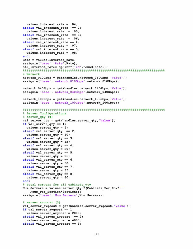
112
values.interest_rate = .04;
elseif val_interest_rate == 2;
values.interest_rate = .05;
elseif val_interest_rate == 3;
values.interest_rate = .06;
elseif val_interest_rate == 4;
values.interest_rate = .07;
elseif val_interest_rate == 5;
values.interest_rate = .08;
end;
Rate = values.interest_rate;
assignin('base','Rate',Rate);
str_interest_rate= sprintf('%d',round(Rate));
%%%%%%%%%%%%%%%%%%%%%%%%%%%%%%%%%%%%%%%%%%%%%%%%%%%%%%%%%%%%%%%%%%%%%%%%%%%
% Network
network_010Gbps = get(handles.network_010Gbps,'Value');
assignin('base','network_010Gbps',network_010Gbps);
network_040Gbps = get(handles.network_040Gbps,'Value');
assignin('base','network_040Gbps',network_040Gbps);
network_100Gbps = get(handles.network_100Gbps,'Value');
assignin('base','network_100Gbps',network_100Gbps);
%%%%%%%%%%%%%%%%%%%%%%%%%%%%%%%%%%%%%%%%%%%%%%%%%%%%%%%%%%%%%%%%%%%%%%%%%%%
% Server Configurations
% server_qty (#)
val_server_qty = get(handles.server_qty,'Value');
if val_server_qty == 1;
values.server_qty = 5;
elseif val_server_qty == 2;
values.server_qty = 10;
elseif val_server_qty == 3;
values.server_qty = 15;
elseif val_server_qty == 4;
values.server_qty = 20;
elseif val_server_qty == 5;
values.server_qty = 25;
elseif val_server_qty == 6;
values.server_qty = 30;
elseif val_server_qty == 7;
values.server_qty = 35;
elseif val_server_qty == 8;
values.server_qty = 40;
end;
% total servers for all cabinets_qty
Num_Servers = values.server_qty.*(Cabinets_Per_Row*...
Rows_Per_Section*Sections);
assignin('base','Num_Servers',Num_Servers);
% server_avgcost ($)
val_server_avgcost = get(handles.server_avgcost,'Value');
if val_server_avgcost == 1;
values.server_avgcost = 2000;
elseif val_server_avgcost == 2;
values.server_avgcost = 4000;
elseif val_server_avgcost == 3;
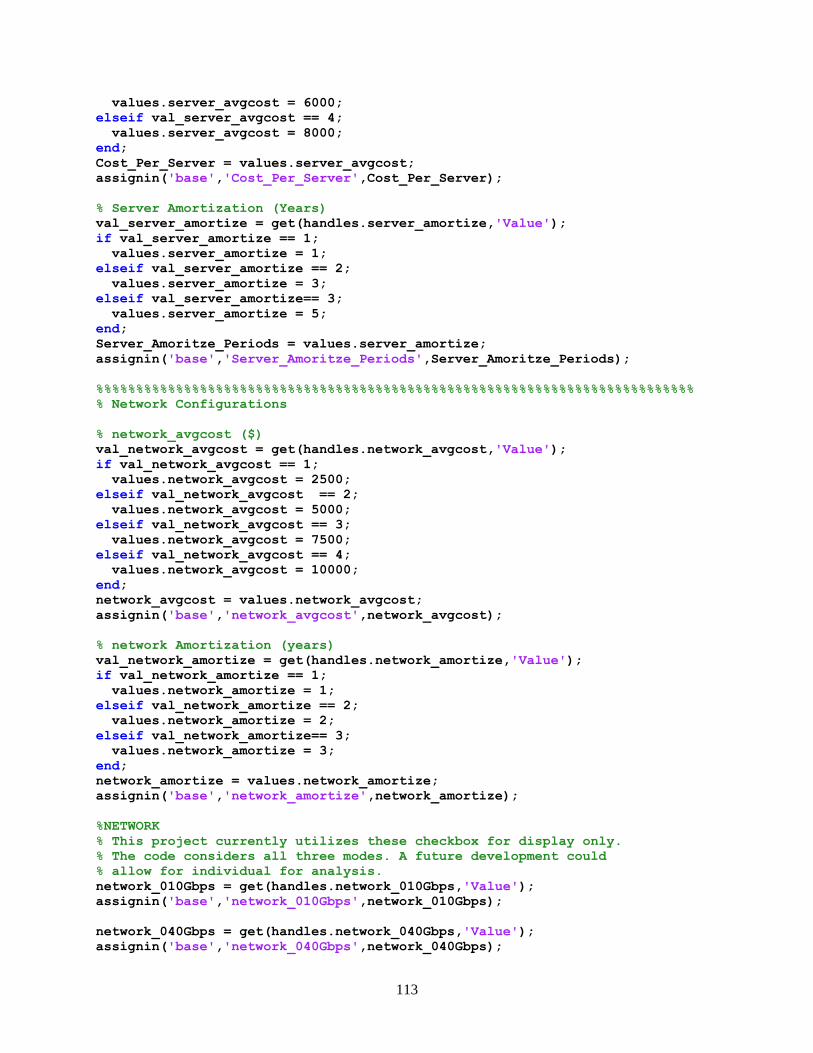
113
values.server_avgcost = 6000;
elseif val_server_avgcost == 4;
values.server_avgcost = 8000;
end;
Cost_Per_Server = values.server_avgcost;
assignin('base','Cost_Per_Server',Cost_Per_Server);
% Server Amortization (Years)
val_server_amortize = get(handles.server_amortize,'Value');
if val_server_amortize == 1;
values.server_amortize = 1;
elseif val_server_amortize == 2;
values.server_amortize = 3;
elseif val_server_amortize== 3;
values.server_amortize = 5;
end;
Server_Amoritze_Periods = values.server_amortize;
assignin('base','Server_Amoritze_Periods',Server_Amoritze_Periods);
%%%%%%%%%%%%%%%%%%%%%%%%%%%%%%%%%%%%%%%%%%%%%%%%%%%%%%%%%%%%%%%%%%%%%%%%%%%
% Network Configurations
% network_avgcost ($)
val_network_avgcost = get(handles.network_avgcost,'Value');
if val_network_avgcost == 1;
values.network_avgcost = 2500;
elseif val_network_avgcost == 2;
values.network_avgcost = 5000;
elseif val_network_avgcost == 3;
values.network_avgcost = 7500;
elseif val_network_avgcost == 4;
values.network_avgcost = 10000;
end;
network_avgcost = values.network_avgcost;
assignin('base','network_avgcost',network_avgcost);
% network Amortization (years)
val_network_amortize = get(handles.network_amortize,'Value');
if val_network_amortize == 1;
values.network_amortize = 1;
elseif val_network_amortize == 2;
values.network_amortize = 2;
elseif val_network_amortize== 3;
values.network_amortize = 3;
end;
network_amortize = values.network_amortize;
assignin('base','network_amortize',network_amortize);
%NETWORK
% This project currently utilizes these checkbox for display only.
% The code considers all three modes. A future development could
% allow for individual for analysis.
network_010Gbps = get(handles.network_010Gbps,'Value');
assignin('base','network_010Gbps',network_010Gbps);
network_040Gbps = get(handles.network_040Gbps,'Value');
assignin('base','network_040Gbps',network_040Gbps);

114
network_100Gbps = get(handles.network_100Gbps,'Value');
assignin('base','network_100Gbps',network_100Gbps);
%%%%%%%%%%%%%%%%%%%%%%%%%%%%%%%%%%%%%%%%%%%%%%%%%%%%%%%%%%%%%%%%%%%%%%%%%%%
% Data Configurations
% bandwidth_per_user
val_bandwidth_per_user = get(handles.bandwidth_per_user,'Value');
if val_bandwidth_per_user == 1;
values.bandwidth_per_user = 1;
elseif val_bandwidth_per_user == 2;
values.bandwidth_per_user = 2;
elseif val_bandwidth_per_user == 3;
values.bandwidth_per_user = 10;
elseif val_bandwidth_per_user == 4;
values.bandwidth_per_user = 25;
elseif val_bandwidth_per_user == 5;
values.bandwidth_per_user = 50;
elseif val_bandwidth_per_user == 6;
values.bandwidth_per_user = 100;
end;
bandwidth_per_user = values.bandwidth_per_user;
assignin('base','bandwidth_per_user',bandwidth_per_user);
% Users Load -- How many users expected during regular use
val_efficiency = get(handles.efficiency,'Value');
if val_efficiency == 1;
values.efficiency = .20;
elseif val_efficiency == 2;
values.efficiency = .40;
elseif val_efficiency == 3;
values.efficiency = .60;
elseif val_efficiency == 4;
values.efficiency = .80;
end;
efficiency = values.efficiency;
assignin('base','efficiency',efficiency);
% Price Per Meter for OM3_010G
val_OM3_PricePerMeter_010G = get(handles.OM3_PricePerMeter_010G,'Value');
if val_OM3_PricePerMeter_010G == 1;
values.OM3_PricePerMeter_010G = 1.00;
elseif val_OM3_PricePerMeter_010G == 2;
values.OM3_PricePerMeter_010G = 1.25;
elseif val_OM3_PricePerMeter_010G == 3
values.OM3_PricePerMeter_010G = 1.50;
end;
price_per_meter_010G_OM3 = values.OM3_PricePerMeter_010G;
assignin('base','price_per_meter_010G_OM3',price_per_meter_010G_OM3);
str_price_per_meter_010G_OM3 = sprintf('%d',price_per_meter_010G_OM3);
% Price Per Meter for OM3_040G
val_OM3_PricePerMeter_040G = get(handles.OM3_PricePerMeter_040G,'Value');
if val_OM3_PricePerMeter_040G == 1;
values.OM3_PricePerMeter_040G = 2.00;
elseif val_OM3_PricePerMeter_040G == 2;
values.OM3_PricePerMeter_040G = 2.25;

115
elseif val_OM3_PricePerMeter_040G == 3
values.OM3_PricePerMeter_040G = 2.50;
end;
price_per_meter_040G_OM3 = values.OM3_PricePerMeter_040G;
assignin('base','price_per_meter_040G_OM3',price_per_meter_040G_OM3);
str_price_per_meter_040G_OM3 = sprintf('%d',price_per_meter_040G_OM3);
% Price Per Meter for OM3_100G
val_OM3_PricePerMeter_100G = get(handles.OM3_PricePerMeter_100G,'Value');
if val_OM3_PricePerMeter_100G == 1;
values.OM3_PricePerMeter_100G = 1.00;
elseif val_OM3_PricePerMeter_100G == 2;
values.OM3_PricePerMeter_100G = 2.50;
elseif val_OM3_PricePerMeter_100G == 3
values.OM3_PricePerMeter_100G = 3.50;
end;
price_per_meter_100G_OM3 = values.OM3_PricePerMeter_100G;
assignin('base','price_per_meter_100G_OM3',price_per_meter_100G_OM3);
str_price_per_meter_100G_OM3 = sprintf('%d',price_per_meter_100G_OM3);
% Price Per Meter for OM4_10G
val_OM4_PricePerMeter_010G = get(handles.OM4_PricePerMeter_010G,'Value');
if val_OM4_PricePerMeter_010G == 1;
values.OM4_PricePerMeter_010G = 2.00;
elseif val_OM4_PricePerMeter_010G == 2;
values.OM4_PricePerMeter_010G = 4.50;
elseif val_OM4_PricePerMeter_010G == 3
values.OM4_PricePerMeter_010G = 6.25;
end;
price_per_meter_010G_OM4 = values.OM4_PricePerMeter_010G;
assignin('base','price_per_meter_010G_OM4',price_per_meter_010G_OM4);
str_price_per_meter_010G_OM4 = sprintf('%d',price_per_meter_010G_OM4);
% Price Per Meter for OM4_40G
val_OM4_PricePerMeter_040G = get(handles.OM4_PricePerMeter_040G,'Value');
if val_OM4_PricePerMeter_040G == 1;
values.OM4_PricePerMeter_040G = 2.00;
elseif val_OM4_PricePerMeter_040G == 2;
values.OM4_PricePerMeter_040G = 4.50;
elseif val_OM4_PricePerMeter_040G == 3
values.OM4_PricePerMeter_040G = 6.25;
end;
price_per_meter_040G_OM4 = values.OM4_PricePerMeter_040G;
assignin('base','price_per_meter_040G_OM4',price_per_meter_040G_OM4);
str_price_per_meter_040G_OM4 = sprintf('%d',price_per_meter_040G_OM4);
% Price Per Meter for OM4_10G
val_OM4_PricePerMeter_100G = get(handles.OM4_PricePerMeter_100G,'Value');
if val_OM4_PricePerMeter_100G == 1;
values.OM4_PricePerMeter_100G = 2.00;
elseif val_OM4_PricePerMeter_100G == 2;
values.OM4_PricePerMeter_100G = 4.50;
elseif val_OM4_PricePerMeter_100G == 3
values.OM4_PricePerMeter_100G = 6.25;
end;
price_per_meter_100G_OM4 = values.OM4_PricePerMeter_100G;
assignin('base','price_per_meter_100G_OM4',price_per_meter_100G_OM4);

116
str_price_per_meter_100G_OM4 = sprintf('%d',price_per_meter_100G_OM4);
%%%%%%%%%%%%%%%%%%%%%%%%%%%%%%%%%%%%%%%%%%%%%%%%%%%%%%%%%%%%%%%%%%%%%%%%%%%
%%% Genetic Algorithm Parameters
val_gaparam_popsize = get(handles.gaparam_popsize,'Value');
if val_gaparam_popsize == 1;
values.gaparam_popsize = 50;
elseif val_gaparam_popsize == 2;
values.gaparam_popsize = 100;
elseif val_gaparam_popsize == 3;
values.gaparam_popsize = 150;
elseif val_gaparam_popsize == 4;
values.gaparam_popsize = 200;
end;
gaparam_popsize = values.gaparam_popsize;
assignin('base','gaparam_popsize',gaparam_popsize);
% gaparam_max_gen defines the maximum generations for the GA algorithm
val_gaparam_max_gen = get(handles.gaparam_max_gen,'Value');
if val_gaparam_max_gen == 1;
values.gaparam_max_gen = 100;
elseif val_gaparam_max_gen == 2;
values.gaparam_max_gen = 150;
elseif val_gaparam_max_gen == 3;
values.gaparam_max_gen = 200;
elseif val_gaparam_max_gen == 4;
values.gaparam_max_gen = 250;
end;
gaparam_max_gen = values.gaparam_max_gen;
assignin('base','gaparam_max_gen',gaparam_max_gen);
% gaparam_max_gen defines the maximum generations for the GA algorithm
val_gaparam_stall_gen = get(handles.gaparam_stall_gen,'Value');
if val_gaparam_stall_gen == 1;
values.gaparam_stall_gen = 100;
elseif val_gaparam_stall_gen == 2;
values.gaparam_stall_gen = 150;
elseif val_gaparam_stall_gen == 3;
values.gaparam_stall_gen = 200;
elseif val_gaparam_stall_gen == 4;
values.gaparam_stall_gen = 250;
end;
gaparam_stall_gen = values.gaparam_stall_gen;
assignin('base','gaparam_stall_gen',gaparam_stall_gen);
% gaparam_prob_crossoverfraction (%)
val_gaparam_prob_crossoverfraction = get...
(handles.gaparam_prob_crossoverfraction,'Value');
if val_gaparam_prob_crossoverfraction == 1;
values.gaparam_prob_crossoverfraction = .6;
elseif val_gaparam_prob_crossoverfraction == 2;
values.gaparam_prob_crossoverfraction = 0.7;
elseif val_gaparam_prob_crossoverfraction == 3;
values.gaparam_prob_crossoverfraction = 0.8;
end;
gaparam_prob_crossoverfraction = values.gaparam_prob_crossoverfraction;

117
assignin('base','gaparam_prob_crossoverfraction',...
gaparam_prob_crossoverfraction);
% gaparam_prob_paretofraction (%)
val_gaparam_prob_paretofraction = ...
get(handles.gaparam_prob_paretofraction,'Value');
if val_gaparam_prob_paretofraction == 1;
values.gaparam_prob_paretofraction = .60;
elseif val_gaparam_prob_paretofraction == 2;
values.gaparam_prob_paretofraction = .70;
elseif val_gaparam_prob_paretofraction == 3;
values.gaparam_prob_paretofraction = .80;
end;
gaparam_prob_paretofraction = values.gaparam_prob_paretofraction;
assignin('base','gaparam_prob_paretofraction',gaparam_prob_paretofraction);
%% %%%%%%%%%%%%%%%%%%%%%%%%%%%%%%%%%%%%%%%%%%%%%%%%%%%%%%%%%%%%%%%%%%%%%%%%
%%%%%%%%%%%%%%%%%%%%%%%%%%%%%%%%%%%%%%%%%%%%%%%%%%%%%%%%%%%%%%%%%%%%%%%%%%%
% COMPUTE THE DATA CENTER
%%%%%%%%%%%%%%%%%%%%%%%%%%%%%%%%%%%%%%%%%%%%%%%%%%%%%%%%%%%%%%%%%%%%%%%%%%%
%%%%%%%%%%%%%%%%%%%%%%%%%%%%%%%%%%%%%%%%%%%%%%%%%%%%%%%%%%%%%%%%%%%%%%%%%%%
%%%DATA CENTER COSTS%%%%%%%%%%%%%%%%%%%%%%%%%%%%%%%%%%%%%%%%%%%%%%%%%%%%%%%
% Equations sourced from: James Hamilton
% http://perspectives.mvdirona.com/2008/11...
% /cost-of-power-in-large-scale-data-centers/
% *****************************************************************
% Infrastructure
% [=-PMT(CostOfMoney/12,FacilityAmortization,FacilityCost,0)]
% Add the Project Integraton Costs and Maintenance Costs
Infrastructure = payper(Rate./12, Facility_Amortize_Periods.*12,...
(Cost_of_Facility + Integration_Cost + Maintenance_Cost),0,0);
str_Infrastructure= sprintf('%d',round(Infrastructure));
str_Infrastructure = fliplr(regexprep(fliplr(str_Infrastructure),...
'(\d+\.)?(\d{3})(?=\S+)', '$1$2,'));
% Servers
% [=-PMT(CostOfMoney/12, ServerAmortization, ServerCount*ServerCost, 0)]
Servers = payper(Rate/12, Server_Amoritze_Periods.*12,...
Num_Servers.*Cost_Per_Server, 0,0);
str_Servers= sprintf('%d',round(Servers));
str_Servers = fliplr(regexprep(fliplr(str_Servers),...
'(\d+\.)?(\d{3})(?=\S+)', '$1$2,'));
% TOR Switches Networking
% [=-PMT(CostOfMoney/12, TORSwitchAmortization,...
%TORSwitchCount*TORSwitchCost, 0)]
Num_TOR_Switches = (Sections.*Rows_Per_Section.*...
Cabinets_Per_Row).*2; % two at top of each cabinet
TOR_Switches = payper(Rate./12, network_amortize.*12, ...
Num_TOR_Switches.*network_avgcost, 0,0);
str_TOR_Switches = sprintf('%d',round(TOR_Switches));
str_TOR_Switches = fliplr(regexprep(fliplr(str_TOR_Switches),...
'(\d+\.)?(\d{3})(?=\S+)', '$1$2,'));
% Power & Cooling Infrastructure
% [=InfrastructureMonthly*PowerAndCoolikngInfrastructurePercentage]
Power_Cooling_Infrastructure= (Infrastructure.*...
Power_Cooling_Infrastructure_Percentage);

118
str_Power_Cooling_Infrastructure= sprintf('%d',...
round(Power_Cooling_Infrastructure));
str_Power_Cooling_Infrastructure = ...
fliplr(regexprep(fliplr(str_Power_Cooling_Infrastructure),...
'(\d+\.)?(\d{3})(?=\S+)', '$1$2,'));
% Power
% [=MegaWattsCriticalLoad*AveragePowerUsage/1000*PUE*PowerCost*24*365/12]
Power= Mega_WattsCritical_Load*Average_Power_Usage/1000*PUE*...
PowerCost_kwh*24*(365/12);
str_Power= sprintf('%d',round(Power));
str_Power = fliplr(regexprep(fliplr(str_Power), ...
'(\d+\.)?(\d{3})(?=\S+)', '$1$2,'));
% Other Infrastructure
% [=+InfrastructureMonthly-PowerAndCoolingInfrastructureMonthly]
Other_Infrastructure= Infrastructure-Power_Cooling_Infrastructure;
str_Other_Infrastructure= sprintf('%d',round(Other_Infrastructure));
str_Other_Infrastructure = fliplr(regexprep(fliplr...
(str_Other_Infrastructure), '(\d+\.)?(\d{3})(?=\S+)', '$1$2,'));
% Full burdened Power
% [=+PowerAndCoingInfrastructureMonthly+PowerMonthly]
Full_Burdened_Power = Power_Cooling_Infrastructure + Power;
str_Full_Burdened_Power= sprintf('%d',round(Full_Burdened_Power));
str_Full_Burdened_Power = fliplr(regexprep(fliplr...
(str_Full_Burdened_Power), '(\d+\.)?(\d{3})(?=\S+)', '$1$2,'));
assignin('base','Full_Burdened_Power',Full_Burdened_Power);
% Total
Total_Cost = Infrastructure + Servers + TOR_Switches + Power;
str_Total= sprintf('%d',round(Total_Cost));
str_Total = fliplr(regexprep(fliplr(str_Total),...
'(\d+\.)?(\d{3})(?=\S+)', '$1$2,'));
assignin('base','Servers',Servers);
assignin('base','TOR_Switches',TOR_Switches);
assignin('base','Power_Cooling_Infrastructure',...
Power_Cooling_Infrastructure);
assignin('base','Power',Power);
assignin('base','Other_Infrastructure',Other_Infrastructure);
X = [Servers;TOR_Switches;Power_Cooling_Infrastructure;...
Power;Other_Infrastructure];
assignin('base','X',X);
%% %% %%%%%%%%%%%%%%%%%%%%%%%%%%%%%%%%%%%%%%%%%%%%%%%%%%%%%%%%%%%%%%%%%%%%%
% % RUN THE GA CODE HERE %%%%%%%%%%%%%%%%%%%%%%%%%%%%%%%%%%%%%%%%%%%%%%%%%%
% %%%%%%%%%%%%%%%%%%%%%%%%%%%%%%%%%%%%%%%%%%%%%%%%%%%%%%%%%%%%%%%%%%%%%%%%%
%%
% Problem setup
numberOfVariables = 6; % Number of decision variables
% Bound Constraints
lb = [1, 1, 1, 1, 1, 1]; % Lower bound
ub = [300, 100, 100, 550, 150, 150]; % Upper bound
Bound = [lb; ub];
VLB=lb;

119
VUB=ub;
% i=1;
% j=1;
% k=1;
%%Solve the problem without integer constraints
options = gaoptimset('PopulationSize',gaparam_popsize,...
'CreationFcn', @int_pop,...
'MutationFcn', @int_mutation,...
'CrossoverFcn', @int_crossoverarithmetic,...
'StallGenLimit', gaparam_stall_gen,...
'Generations', gaparam_max_gen,...
'PopInitRange', Bound,...
'Display','none',...
'ParetoFraction',gaparam_prob_paretofraction,...
'CrossoverFraction',gaparam_prob_crossoverfraction);
%%%%% DEFINE PARAMETERS%%%%%%%%%%%%%%%%%%%%%%%%%%%%%%%%%%%%%%%%%%%%%%%%
sections = Sections; %% GUI INPUT
rows = Rows_Per_Section; %% GUI INPUT
cabs_per_row = Cabinets_Per_Row; %% GUI INPUT
user_Mbps = bandwidth_per_user; %% GUI INPUT
servers_per_cabinet = values.server_qty; %% GUI INPUT
TOR_switch_cost = payper(Rate./12,network_amortize.*12,...
network_avgcost,0,0); %% GUI INPUT
users_bw = bandwidth_per_user; % measure of MBps %% GUI INPUT
efficiency = efficiency; % efficiency of load relative to max capacity.
distance_from_core = 10;
horizontal = 4 ;
cabinet_width = 4;
vertical = 3;
aisle_width = 5;
%%%%%%%%%
max_distance_010G_OM3 = 330; % meters as defined per Corning
max_distance_040G_OM3 = 100; % meters as defined per Corning
max_distance_100G_OM3 = 100; % meters as defined per Corning
max_distance_010G_OM4 = 550; % meters as defined per Corning
max_distance_040G_OM4 = 150; % meters as defined per Corning
max_distance_100G_OM4 = 150; % meters as defined per Corning
%%%%%%%%%
gigabit2bit = 10^9; % 1 giga(bit) to bits
speed_010G_OM3_Bits = 10*gigabit2bit;
speed_040G_OM3_Bits = 40*gigabit2bit;
speed_100G_OM3_Bits = 100*gigabit2bit;
speed_010G_OM4_Bits = 10*gigabit2bit;
speed_040G_OM4_Bits = 40*gigabit2bit;
speed_100G_OM4_Bits = 100*gigabit2bit;
%%%%%%%%%
intercabinet_distance = 2; % assume 2 meters of fiber inside the cabinets
ports_per_server = 2; % assume 2 ports per server
TOR_per_cabinet = 2; % assume 2 TOR switches at Top of Rack (TOR)
%%%%%%%%%%END PARAMETERS DEFINITION%%%%%%%%%%%%%%%%%%%%%%%%%%%%%%%%%%%%%%%
% Define the functions for LifeCycle Costs, Capacity and QFactor
funLCC = @(x)compute_Fitness_v44_LCC(x,sections,rows,...
cabs_per_row,Full_Burdened_Power,price_per_meter_010G_OM3,...
price_per_meter_040G_OM3,price_per_meter_100G_OM3,...

120
price_per_meter_010G_OM4,price_per_meter_040G_OM4,...
price_per_meter_100G_OM4,servers_per_cabinet,...
Cost_Per_Server, ports_per_server,intercabinet_distance,...
TOR_per_cabinet,TOR_switch_cost)
funCapacity = @(x)compute_Fitness_v44_Capacity(x,...
efficiency,max_distance_010G_OM3,max_distance_040G_OM3,...
max_distance_100G_OM3,max_distance_010G_OM4,max_distance_040G_OM4,...
max_distance_100G_OM4,users_bw);
funQfactor = @(x)compute_Fitness_v44_Qfactor(x);
%% Run the MOGA
tic;
fprintf('Processing...\n');
[x1,fval1] = gamultiobj(funLCC,...
numberOfVariables, [], [], [], [], lb, ub, options);
fprintf('Processing...\n');
[x2,fval2] = gamultiobj(funCapacity,...
numberOfVariables, [], [], [], [], lb, ub, options);
fprintf('Processing...\n');
[x3,fval3] = gamultiobj(funQfactor,...
numberOfVariables, [], [], [], [], lb, ub, options);
%%
%Process to ensure FVALS are the same size.
while size(fval1(:),1 )~= size(fval2(:),1) || size(fval1(:),1)...
~= size(fval3(:),1) || size(fval2(:),1) ~= size(fval3(:),1);
fprintf('Processing...\n');
[x1,fval1] = gamultiobj(funLCC,...
numberOfVariables, [], [], [], [], lb, ub, options);
fprintf('Processing...\n');
[x2,fval2] = gamultiobj(funCapacity,...
numberOfVariables, [], [], [], [], lb, ub, options);
fprintf('Processing...\n');
[x3,fval3] = gamultiobj(funQfactor,...
numberOfVariables, [], [], [], [], lb, ub, options);
end
%
%% Setup the Pareto Matrix
OM3_10G = [fval1(:,1) -fval2(:,1) -fval3(:,1)];
OM3_40G = [fval1(:,2) -fval2(:,2) -fval3(:,2)];
OM3_100G = [fval1(:,3) -fval2(:,3) -fval3(:,3)];
OM4_10G = [fval1(:,4) -fval2(:,4) -fval3(:,4)];
OM4_40G = [fval1(:,5) -fval2(:,5) -fval3(:,5)];
OM4_100G = [fval1(:,6) -fval2(:,6) -fval3(:,6)];
Pareto = [OM3_10G;OM3_40G;OM3_100G;OM4_10G;OM4_40G;OM4_100G];
%% Clear and reset the axes
handles.axes32 = gca; % essential to remind otherwise lost with subplots.
%http://www.mathworks.com/matlabcentral/answers/...
% 48256-axes-problem-in-matlab-gui

121
cla(handles.axes32,'reset');
axes(handles.axes32);
%% %%%%%%%%%%%%%%%%%%%%%%%%%%%%%%%%%%%%%%%%%%%%%%%%%%%%%%%%%%%%%%%%%%%%%%%%
% %Plot B: Cost vs Distance
%%%%%%%%%%%%%%%%%%%%%%%%%%%%%%%%%%%%%%%%%%%%%%%%%%%%%%%%%%%%%%%%%%%%%%%%%%%
h233 = subplot(2,3,3);
cla(h233,'reset');
subplot(2,3,3);
p = get(h233,'position');
p(1) = p(1)*1.02; % Add 0 percent to x
p(2) = p(2)*1.0; % Add 0 percent to y
p(3) = p(3)*1.35; % Add 20 percent to width
p(4) = p(4)*1.10; % Add 10 percent to height
set(h233, 'position', p);
% Cost vs Distance
fval1Pareto(:,1)= [x1(:,1);x1(:,2);x1(:,3);x1(:,4);x1(:,5);x1(:,6)];
fval1Pareto(:,2)= -[fval1(:,1);fval1(:,2);fval1(:,3);fval1(:,4);...
fval1(:,5);fval1(:,6)];
Pareto_x1_vs_fval1 = zeros(size(fval1Pareto,1),2);
Pareto_x1_vs_fval1_sorted= zeros(size(fval1Pareto,1),2);
a=zeros(size(fval1Pareto,1),2);
x=zeros(size(fval1Pareto,1),1);
y=zeros(size(fval1Pareto,1),1);
Pareto_x1_vs_fval1 = [fval1Pareto(:,1) fval1Pareto(:,2)];
Pareto_x1_vs_fval1_sorted = sortrows(Pareto_x1_vs_fval1,2);
a=Pareto_x1_vs_fval1_sorted ;
x= fval1Pareto(:,1);
y= fval1Pareto(:,2);
N = size(Pareto_x1_vs_fval1_sorted,1);
compare_matrix= gpuArray(size(N,N)); % GPU array
compare_matrix = cell2mat(arrayfun(@(ii) all(bsxfun(@(x,y)... % RUN GPU
x<=min(y),a,a(ii,:)),2),1:N,'uni',false)); % RUN GPU
compare_matrix(1:N+1:N^2)=false; % set diagonal to false
dominated_idxs = size(size(fval1Pareto,1),1);
dominated_idxs = any(compare_matrix,2);
a(dominated_idxs ,:) = [];
hold on;
plot(a(:,1),-a(:,2),...
'MarkerFaceColor',[1 1 1],'MarkerEdgeColor',[0 .8 0],...
'MarkerSize',10,...
'Marker','square',...
'LineWidth',1,...
'Color',[1 0 0]);
set(gca,'XScale','log');
ParetoLCC_X = a(:,1);
ParetoLCC_Y = -a(:,2);
hold on;
scatter(x1(:,1),fval1(:,1),'ok','Display','10G OM3',...
'MarkerEdgeColor',[0 0 0]); %black
scatter(x1(:,2),fval1(:,2),'ob','Display','40G OM3',...
'MarkerEdgeColor',[0 0 1]); %blue

122
scatter(x1(:,3),fval1(:,3),'om','Display','100G OM3',...
'MarkerEdgeColor',[1 0 1]); %magenta
scatter(x1(:,4),fval1(:,4),'Xk','Display','10G OM4',...
'MarkerEdgeColor',[0 0 0]); %black
scatter(x1(:,5),fval1(:,5),'Xb','Display','40G OM4',...
'MarkerEdgeColor',[0 0 1]); %blue
scatter(x1(:,6),fval1(:,6),'Xm','Display','100G OM4',...
'MarkerEdgeColor',[1 0 1]); %magenta
title({'Cost ($) vs Distance(m)'},'Color','blue');
xlabel({'Distance (m)'});
ylabel({'Cost ($)'});
text(-.11,1.04,'(B)','Units', 'Normalized', 'VerticalAlignment',...
'Bottom','color','k','fontw','b','FontSize',8)
set(gca,'XScale','log');
set(gca,'FontSize',7);
set(gcf,'Color','w');
legendsize= legend('Pareto','OM3 10G','OM3 40G','OM3 100G','OM4 10G',...
'OM4 40G','OM4 100G', 'Location','northwest');
set(legendsize,'FontSize',7)
grid on;
box on;
%
%% %%%%%%%%%%%%%%%%%%%%%%%%%%%%%%%%%%%%%%%%%%%%%%%%%%%%%%%%%%%%%%%%%%%%%%%%
% Plot C: Capacity vs Distance
%%%%%%%%%%%%%%%%%%%%%%%%%%%%%%%%%%%%%%%%%%%%%%%%%%%%%%%%%%%%%%%%%%%%%%%%%%%
h235 = subplot(2,3,5);
cla(h235,'reset');
subplot(2,3,5);
p = get(h235,'position');
p(1) = p(1)*(.85); % Substract 15% to x
p(2) = p(2)*.7; % Substract 30% to y
p(3) = p(3)*1.4; % Add 40% to width
p(4) = p(4)*1.1; % Add 10% to height
set(h235, 'position', p);
% Capacity vs Distance
fval2Pareto(:,1)= [x2(:,1);x2(:,2);x2(:,3);x2(:,4);x2(:,5);x2(:,6)];
fval2Pareto(:,2)= [fval2(:,1);fval2(:,2);fval2(:,3);fval2(:,4);...
fval2(:,5);fval2(:,6)];
Pareto_x2_vs_fval2 = zeros(size(fval2Pareto,1),2);
Pareto_x2_vs_fval2_sorted= zeros(size(fval2Pareto,1),2);
a=zeros(size(fval2Pareto,1),2);
x=zeros(size(fval2Pareto,1),1);
y=zeros(size(fval2Pareto,1),1);
Pareto_x2_vs_fval2 = [fval2Pareto(:,1) -fval2Pareto(:,2)];
Pareto_x2_vs_fval2_sorted = sortrows(Pareto_x2_vs_fval2,1);
a=Pareto_x2_vs_fval2_sorted ;

123
x= fval2Pareto(:,1);
y= -fval2Pareto(:,2);
N = size(Pareto_x2_vs_fval2_sorted,1);
compare_matrix= gpuArray(size(N,N)); % GPU array
compare_matrix = cell2mat(arrayfun(@(ii) all(bsxfun(@(x,y)... % RUN GPU
x<=min(y),a,a(ii,:)),2),1:N,'uni',false)); % RUN GPU
compare_matrix(1:N+1:N^2)=false; % set diagonal to false
dominated_idxs = size(size(fval2Pareto,1),1);
dominated_idxs = any(compare_matrix,2);
a(dominated_idxs ,:) = [];
hold on;
plot(a(:,1),a(:,2),...
'MarkerFaceColor',[1 1 1],'MarkerEdgeColor',[0 .8 0],...
'MarkerSize',10,...
'Marker','square',...
'LineWidth',1,...
'Color',[1 0 0]);
ParetoCapacity_X = a(:,1);
ParetoCapacity_Y = a(:,2);
hold on;
scatter(x2(:,1),-fval2(:,1),'ok','Display','10G OM3',...
'MarkerEdgeColor',[0 0 0]);%black
scatter(x2(:,2),-fval2(:,2),'ob','Display','40G OM3',...
'MarkerEdgeColor',[0 0 1]);%blue
scatter(x2(:,3),-fval2(:,3),'om','Display','100G OM3',...
'MarkerEdgeColor',[1 0 1]); %magenta
scatter(x2(:,4),-fval2(:,4),'Xk','Display','10G OM4',...
'MarkerEdgeColor',[0 0 0]);%black
scatter(x2(:,5),-fval2(:,5),'Xb','Display','40G OM4',...
'MarkerEdgeColor',[0 0 1]);%blue
scatter(x2(:,6),-fval2(:,6),'Xm','Display','100G OM4',...
'MarkerEdgeColor',[1 0 1]); %magenta
title({'Capacity (users) vs. Distance(m)'},'Color','blue');
xlabel({'Distance (m)'});
ylabel({'Capacity (users)'});
text(-.11,1.04,'(C)','Units', 'Normalized', 'VerticalAlignment',...
'Bottom','color','k','fontw','b','FontSize',8)
set(gca,'XScale','log');
set(gca,'FontSize',7);
set(gcf,'Color','w');
grid on;
box on;
%
%% %%%%%%%%%%%%%%%%%%%%%%%%%%%%%%%%%%%%%%%%%%%%%%%%%%%%%%%%%%%%%%%%%%%%%%%%
% Plot D: Qfactor vs Distance
%%%%%%%%%%%%%%%%%%%%%%%%%%%%%%%%%%%%%%%%%%%%%%%%%%%%%%%%%%%%%%%%%%%%%%%%%%%
h236 = subplot(2,3,6);
cla(h236);
p = get(h236,'position');
p(1) = p(1)*1.02; % Add 2 percent to x
p(2) = p(2)*.7; % Add -30 percent to y
p(3) = p(3)*1.35; % Add 35 percent to width

124
p(4) = p(4)*1.10; % Add 10 percent to height
set(h236, 'position', p);
% Qfactor vs Distance
fval3Pareto(:,1)= [x3(:,1);x3(:,2);x3(:,3);x3(:,4);x3(:,5);x3(:,6)];
fval3Pareto(:,2)= -[fval3(:,1);fval3(:,2);fval3(:,3);fval3(:,4);...
fval3(:,5);fval3(:,6)];
Pareto_x3_vs_fval3 = zeros(size(fval3Pareto,1),2);
Pareto_x3_vs_fval3_sorted= zeros(size(fval3Pareto,1),2);
a=zeros(size(fval3Pareto,1),2);
x=zeros(size(fval3Pareto,1),1);
y=zeros(size(fval3Pareto,1),1);
Pareto_x3_vs_fval3 = [fval3Pareto(:,1) fval3Pareto(:,2)];
Pareto_x3_vs_fval3_sorted = sortrows(Pareto_x3_vs_fval3,2);
a=Pareto_x3_vs_fval3_sorted ;
x= fval3Pareto(:,1);
y= fval3Pareto(:,2);
N = size(Pareto_x3_vs_fval3_sorted,1);
compare_matrix= gpuArray(size(N,N)); % GPU array
compare_matrix = cell2mat(arrayfun(@(ii) all(bsxfun(@(x,y)... % RUN GPU
x<=min(y),a,a(ii,:)),2),1:N,'uni',false)); % RUN GPU
compare_matrix(1:N+1:N^2)=false; % set diagonal to false
dominated_idxs = size(size(fval3Pareto,1),1);
dominated_idxs = any(compare_matrix,2);
a(dominated_idxs ,:) = [];
hold on;
plot(a(:,1),a(:,2),...
'MarkerFaceColor',[1 1 1],'MarkerEdgeColor',[0 .8 0],...
'MarkerSize',10,...
'Marker','square',...
'LineWidth',1,...
'Color',[1 0 0]);
ParetoQfactor_X = a(:,1);
ParetoQfactor_Y = a(:,2);
hold on;
scatter(x3(:,1),-fval3(:,1),'ok','Display','10G OM3',...
'MarkerEdgeColor',[0 0 0]);
scatter(x3(:,2),-fval3(:,2),'ob','Display','40G OM3',...
'MarkerEdgeColor',[0 0 1]);
scatter(x3(:,3),-fval3(:,3),'om','Display','100G OM3',...
'MarkerEdgeColor',[1 0 1]);
scatter(x3(:,4),-fval3(:,4),'Xk','Display','10G OM4',...
'MarkerEdgeColor',[0 0 0]);
scatter(x3(:,5),-fval3(:,5),'Xb','Display','40G OM4',...
'MarkerEdgeColor',[0 0 1]);
scatter(x3(:,6),-fval3(:,6),'Xm','Display','100G OM4',...
'MarkerEdgeColor',[1 0 1]);
title({'Qfactor vs Distance(m)'},'Color','blue');
xlabel({'Distance (m)'});
ylabel({'Qfactor'});
text(-.11,1.04,'(D)','Units', 'Normalized', 'VerticalAlignment',...

125
'Bottom','color','k','fontw','b','FontSize',8)
set(gca,'XScale','log');
set(gca,'FontSize',7);
set(gcf,'Color','w');
grid on;
box on;
%
%% %%%%%%%%%%%%%%%%%%%%%%%%%%%%%%%%%%%%%%%%%%%%%%%%%%%%%%%%%%%%%%%%%%%%%%%%
% Plot A: Pareto Fronter for Qfactor vs Capacity vs Cost
%%%%%%%%%%%%%%%%%%%%%%%%%%%%%%%%%%%%%%%%%%%%%%%%%%%%%%%%%%%%%%%%%%%%%%%%%%%
h232 = subplot(2,3,2);
cla(h232);
subplot(2,3,2);
p = get(h232,'position');
p(1) = p(1)*(.85); % Substract 5 percent to x
p(2) = p(2)*1.0; % Add 0 percent to y
p(3) = p(3)*1.2; % Add 0 percent to width
p(4) = p(4)*1.1; % Add 0 percent to height
set(h232, 'position', p);
set(h232,'xlim',[min(+fval1(:)) max(+fval1(:))]);
set(h232,'ylim',[min(-fval2(:)) max(-fval2(:))]);
set(h232,'zlim',[min(-fval3(:)) max(-fval3(:))]);
gvx = ParetoLCC_Y;
gvy = ParetoCapacity_Y;
gvz = ParetoQfactor_Y;
m = size(gvx,1);
n = size(gvy,1);
q = size(gvz,1);
A = [m n q];
scale_gvx = size(gvx,1)/ min(A); % SCALE FACTOR FOR HORZCAT PURPOSES
scale_gvy = size(gvy,1)/ min(A); % SCALE FACTOR FOR HORZCAT PURPOSES
scale_gvz = size(gvz,1)/ min(A); % SCALE FACTOR FOR HORZCAT PURPOSES
gvxA = gvx;
gvyA = gvy;
gvzA = gvz;
gvxA = gvx(1:scale_gvx:end); %RESCALE THE MATRIX
gvyA = gvy(1:scale_gvy:end); %RESCALE THE MATRIX
gvzA = gvz(1:scale_gvz:end); %RESCALE THE MATRIX
hold on
plot3(gvxA,gvyA,gvzA,'-s','Color','red','Display','Pareto')
title({'Pareto: Qfactor vs. Capacity vs. Cost'},'Color','blue');
xlabel({'Cost'},'FontWeight','bold');
ylabel({'Capacity'},'FontWeight','bold');
zlabel({'Qfactor'},'FontWeight','bold');
set(gca,'FontSize',7);
set(gcf,'Color','w');

126
set(gca,'LooseInset',get(gca,'TightInset'))
text(-.11,1.04,'(A)','Units', 'Normalized', 'VerticalAlignment',...
'Bottom','color','k','fontw','b','FontSize',8)
legend('Pareto');
legendPlotA = legend('Pareto','Location','northeast');
set(legendPlotA,'FontSize',10)
grid on;
box on;
view([120 10]);
%%%%%%%%%%%%%%%%%%%%%%%%%%%%%%%%%%%%%%%%%%%%%%%%%%%%%%%%%%%%%%%%%%%%%%%%%%%
% PIE CHART %%%%%%%%%%%%%%%%%%%%%%%%%%%%%%%%%%%
% in row 1 position 1
h231 = subaxis(2,3,1,'MarginTop',-.01,'MarginBottom',.02,...
'PaddingBottom',.1,'ML',.1,'MR',.2,'SpacingHoriz',.125,...
'SpacingVert',.125);
cla(h231);
subaxis(2,3,1,'MarginTop',-.01,'MarginBottom',.02,'PaddingBottom',.1,...
'ML',.1,'MR',.2,'SpacingHoriz',.125,'SpacingVert',.125);
h = pie(X);
hText = findobj(h,'Type','text'); % text object handles
set(hText(1),'Fontsize',7);
set(hText(2),'Fontsize',7);
set(hText(3),'Fontsize',7);
set(hText(4),'Fontsize',7);
set(hText(5),'Fontsize',7);
percentValues = get(hText,'String'); % percent values
str = {'Servers: ';'Switches: ';'P&C: ';'Power: ';'Other: '}; % strings
combinedstrings = strcat(str,percentValues); % strings and percent values
oldExtents_cell = get(hText,'Extent'); % cell array
oldExtents = cell2mat(oldExtents_cell); % numeric array
hText(1).String = combinedstrings(1);
hText(2).String = combinedstrings(2);
hText(3).String = combinedstrings(3);
hText(4).String = combinedstrings(4);
hText(5).String = combinedstrings(5);
newExtents_cell = get(hText,'Extent'); % cell array
newExtents = cell2mat(newExtents_cell); % numeric array
width_change = newExtents(:,3)-oldExtents(:,3);
signValues = sign(oldExtents(:,1));
offset = signValues.*(width_change/2);
textPositions_cell = get(hText,{'Position'}); % cell array
textPositions = cell2mat(textPositions_cell); % numeric array
textPositions(:,1) = textPositions(:,1) + offset; % add offset
hText(1).Position = textPositions(1,:);
hText(2).Position = textPositions(2,:);
hText(3).Position = textPositions(3,:);
hText(4).Position = textPositions(4,:);
hText(5).Position = textPositions(5,:);
title('Data Center Costs','FontSize',8,'Color','blue','FontWeight','bold')

127
%% %%%%%%%%%%%%%%%%%%%%%%%%%%%%%%%%%%%%%%%%%%%%%%%%%%%%%%%%%%%%%%%%%%%%%%%%
%%%%Organize the results to command window
fprintf('******************************\n')
disp(['Total (monthly): $',str_Total])
fprintf('******************************\n')
disp(['Infrastructure $',str_Infrastructure])
disp(['Servers: $',str_Servers])
disp(['Power Cooling_Infrastructure: $',str_Power_Cooling_Infrastructure])
disp(['Power: $',str_Power])
disp(['Other Infrastructure: $',str_Other_Infrastructure])
disp(['Fully Burdened Power: $',str_Full_Burdened_Power])
fprintf('******************************\n')
%%%%%%%%%%%%%%%%%%%%%%%%%%%%%%%%%%%%%%%%%%%%%%%%%%%%%%%%%%%%%%%%%%%%%%%%%%%
%DATA TABLE GUI
%%%%%%%%%%%%%%%%%%%%%%%%%%%%%%%%%%%%%%%%%%%%%%%%%%%%%%%%%%%%%%%%%%%%%%%%%%%
colnames = {'Parameter','Result'};
%Table Table_GUI
x01={'Total LCC($)[monthly]'};
y01=str_Total;
x02={'Infra.($)'};
y02=str_Infrastructure;
x03={'Servers($)'};
y03=str_Servers;
x04={'Power Cooling($)'};
y04=str_Power;
x05={'Other Infra.($)'};
y05= str_Other_Infrastructure;
x06= {'Burdened Power ($)'};
y06= str_Full_Burdened_Power;
x07 = {'PUE'};
y07 = PUE;
x08 = {'$/kwh'};
y08 = PowerCost_kwh;
x09 = {'Critical Load (MW)'};
y09 = Mega_WattsCritical_Load./10^6;
x10 = {'Amortize (Yrs)'};
y10 = Facility_Amortize_Periods;
x11 = {'----------'};
y11 = {'---'};
x12 = {'Sections'};
y12= str_sections;
x13 = {'Rows'};
y13 = str_rows;

128
x14 = {'Cabinet/Row'};
y14 = str_cabinets;
x15 = {'Architecture'};
y15 = 'TOR';
%
x16 = {'----------'};
y16 = {'---'};
cputime = toc;
x17 = {'CPUtime (s)'};
y17 = cputime;
% Build GUI Tables
Data1=[x01,y01;x02,y02;x03,y03;x04,y04;x05,y05;x06,y06;x07,y07;...
x08,y08;x09,y09;x10,y10;x11,y11;x12,y12;x13,y13;x14,y14;x15,y15;...
x16,y16;x17,y17];
% Display the results to the GUI table
set(handles.output_table_GUI_01,'data',...
[x01,y01;x02,y02;x03,y03;x04,y04;...
x05,y05;x06,y06;x07,y07;x08,y08;x09,y09;x10,y10;...
x11,y11;x12,y12;x13,y13;x14,y14;x15,y15;x16,y16;...
x17,y17],'ColumnName',colnames);
%%%%%%%%%%%%%%%%%%%%%%%%%%%%%%%%%%%%%%%%%%%%%%%%%%%%%%%%%%%%%%%%%%%%%%%%%%%
%%%%%%%%%%%%%%%%%%%%%%%%%%%%%%%%%%%%%%%%%%%%%%%%%%%%%%%%%%%%%%%%%%%%%%%%%%%

129
5.1.2 function [LCC] = computeLCC
function [J1_LCC] = compute_Fitness_v44_LCC(x,sections,rows,...
cabs_per_row,Full_Burdened_Power,price_per_meter_010G_OM3,...
price_per_meter_040G_OM3,price_per_meter_100G_OM3,...
price_per_meter_010G_OM4,price_per_meter_040G_OM4,...
price_per_meter_100G_OM4,servers_per_cabinet,...
Cost_Per_Server, ports_per_server,intercabinet_distance,...
TOR_per_cabinet,TOR_switch_cost)
x(1) = x(:,1); % Vectorize using columns
x(2) = x(:,2); % Vectorize using columns
x(3) = x(:,3); % Vectorize using columns
x(4) = x(:,4); % Vectorize using columns
x(5) = x(:,5); % Vectorize using columns
x(6) = x(:,6); % Vectorize using columns
AvgPowerPerCabinetCost = Full_Burdened_Power./(sections.*rows.*cabs_per_row);
ServerCosts = servers_per_cabinet.*Cost_Per_Server;
CabinetCableCosts = servers_per_cabinet.*ports_per_server.*...
intercabinet_distance;
%010G_OM3
J1_LCC(1) = sections.*(...
x(1).*price_per_meter_010G_OM3.*TOR_per_cabinet + ...
TOR_per_cabinet.*TOR_switch_cost + ...
CabinetCableCosts.*price_per_meter_010G_OM3 +...
ServerCosts + ...
AvgPowerPerCabinetCost);
%040_OM3
J1_LCC(2) = sections.*(...
x(2).*price_per_meter_040G_OM3.*TOR_per_cabinet + ...
TOR_per_cabinet.*TOR_switch_cost + ...
CabinetCableCosts.*price_per_meter_040G_OM3 +...
ServerCosts + ...
AvgPowerPerCabinetCost);
%100G_OM3
J1_LCC(3) = sections.*(...
x(3).*price_per_meter_100G_OM3.*TOR_per_cabinet + ...
TOR_per_cabinet.*TOR_switch_cost + ...
CabinetCableCosts.*price_per_meter_100G_OM3 +...
ServerCosts + ...
AvgPowerPerCabinetCost);
%010G_OM4
J1_LCC(4) = sections.*(...
x(4).*price_per_meter_010G_OM4.*TOR_per_cabinet + ...
TOR_per_cabinet.*TOR_switch_cost + ...
CabinetCableCosts.*price_per_meter_010G_OM4 +...
ServerCosts + ...
AvgPowerPerCabinetCost);
%040G_OM4
J1_LCC(5) = sections.*(...
130
x(5).*price_per_meter_040G_OM4.*TOR_per_cabinet + ...
TOR_per_cabinet.*TOR_switch_cost + ...
CabinetCableCosts.*price_per_meter_040G_OM4 +...
ServerCosts + ...
AvgPowerPerCabinetCost);
%100G_OM4
J1_LCC(6) = sections.*(...
x(6).*price_per_meter_100G_OM4.*TOR_per_cabinet + ...
TOR_per_cabinet.*TOR_switch_cost + ...
CabinetCableCosts.*price_per_meter_100G_OM4 +...
ServerCosts + ...
AvgPowerPerCabinetCost);

131
5.1.3 function[Capacity] = computeCapacity
function [J2_Capacity] = compute_Fitness_v42_Capacity(x,...
efficiency,max_distance_010G_OM3,max_distance_040G_OM3,...
max_distance_100G_OM3,max_distance_010G_OM4,max_distance_040G_OM4,...
max_distance_100G_OM4,users_bw);
x(1) = x(:,1); % Vectorize using columns
x(2) = x(:,2); % Vectorize using columns
x(3) = x(:,3); % Vectorize using columns
x(4) = x(:,4); % Vectorize using columns
x(5) = x(:,5); % Vectorize using columns
x(6) = x(:,6); % Vectorize using columns
% Max capacity of users at network efficiency
users_Gbps = users_bw./10^3;
Max_Capacity_010G_OM3 = (010/users_Gbps).*efficiency;
Max_Capacity_040G_OM3 = (040/users_Gbps).*efficiency;
Max_Capacity_100G_OM3 = (100/users_Gbps).*efficiency;
Max_Capacity_010G_OM4 = (010/users_Gbps).*efficiency;
Max_Capacity_040G_OM4 = (040/users_Gbps).*efficiency;
Max_Capacity_100G_OM4 = (100/users_Gbps).*efficiency;
%OM3 10G
J2_Capacity(1) = -1.*(Max_Capacity_010G_OM3.*(max_distance_010G_OM3-x(1))...
./max_distance_010G_OM3);
%OM3 40G
J2_Capacity(2) = -1.*(Max_Capacity_040G_OM3.*(max_distance_040G_OM3-x(2))...
./max_distance_040G_OM3);
%OM3 100G
J2_Capacity(3) = -1.*(Max_Capacity_100G_OM3.*(max_distance_100G_OM3-x(3))...
./max_distance_100G_OM3);
%OM4 10G
J2_Capacity(4) = -1.*(Max_Capacity_010G_OM4.*(max_distance_010G_OM4-x(4))...
./max_distance_010G_OM4);
%OM4 40G
J2_Capacity(5) = -1.*(Max_Capacity_040G_OM4.*(max_distance_040G_OM4-x(5))...
./max_distance_040G_OM4);
%OM4 100G
J2_Capacity(6) = -1.*(Max_Capacity_100G_OM4.*(max_distance_100G_OM4-x(6))...
./max_distance_100G_OM4);

132
5.1.4 function [Qfactor] = computeQfactor
function [J3_Qfactor] = compute_Fitness_v42_Qfactor(x);
x(1) = x(:,1); % Vectorize using columns
x(2) = x(:,2); % Vectorize using columns
x(3) = x(:,3); % Vectorize using columns
x(4) = x(:,4); % Vectorize using columns
x(5) = x(:,5); % Vectorize using columns
x(6) = x(:,6); % Vectorize using columns
%%% OM3, Equations 2.5 - 2.7
% Eqn. 2.5, y =.00000*exp(0.07584*x) + 7.87968*exp(-.0001*x)
% Eqn. 2.6, y = 5.47297*exp(-0.12299*x)+7.27510*exp(-0.0004*x)
% Eqn. 2.7, y = 5.59373292*exp(-0.12927862*x)+7.28378306*exp(-0.00042308*x)
%%%%%%%%%
%OM3 10G
%y = 7.37968.*exp(-.000215) Eqn.(2.5)
J3_Qfactor(1) = -1.*(7.37968.*exp(-.000215*x(1)));
%OM3 40G
%y = 5.47297*exp(-0.12299*x) + 7.27510*exp(-0.0004*x) Eqn. 2.6
J3_Qfactor(2) = -1.*((5.47297.*exp(-0.12299.*x(2))...
+7.27510.*exp(-0.0004.*x(2))));
%OM3 100G
%y = 5.59373292*exp(-0.12927862*x)+7.28378306*exp(-0.00042308*x) Eqn 2.7
J3_Qfactor(3) = -1.*((5.59373292.*exp(-0.12927862.*x(3)) ...
+ 7.28378306.*exp(-0.00042308.*x(3))));
%%% OM4, Equations 2.8 - 2.9
% Eqn. 2.8, y = 7.77941*exp(-0.00015*x)+-0.000001*exp(0.021*x)
% Eqn. 2.9, y = 5.08844*exp(-0.04094*x)+7.15245*exp(0.00001*x)
% Eqn. 2.10, y = 4.89846*exp(-0.04601*x)+7.22401*exp(0.0001*x)
%%%%%%%%%
%OM4 10G
%y = 7.77941*exp(-0.00015*x)-0.000001*exp(0.021*x) Eqn. 2.8
J3_Qfactor(4) = -1.*(7.77941.*exp(-0.00015.*x(4)) ...
- 0.000001.*exp(0.021.*x(4)));
%OM4 40G
%y = 5.08844*exp(-0.04094*x) + 7.15245*exp(0.0000004*x) Eqn. 2.9
J3_Qfactor(5) = -1.*(5.08844.*exp(-0.04094.*x(5)) ...
+ 7.15245.*exp(0.0000004.*x(5)));
%OM4 100G
%y = 4.89846*exp(-0.04601*x)+7.22401*exp(-.0000001*x)) Eqn 2.10
J3_Qfactor(6) = -1.*(4.89846.*exp(-0.04601.*x(6)) ...
+ 7.72401.*exp(-0.0000001.*x(6)));

133
5.1.5 function [Population] = int_pop
% File reference: exampleIntGAMULTIOBJ.zip
% http://www.mathworks.com/matlabcentral/answers/103369-is-it-possible-to
% -solve-a-mixed-integer-multi-objective-optimization-...
% -problem-using-global-optimizati
%
% MATLAB Answers™
% Is it possible to solve a mixed-integer multi-objective optimization ...
% problem using Global Optimization Toolbox 3.2.4 (R2013b)?
% Asked by MathWorks Support Team on 25 Oct 2013
function Population = int_pop(GenomeLength, ~, options)
% INT_POP Function that creates an initial population satisfying bounds and
% integer constraints
totalPopulation = sum(options.PopulationSize);
%IntCon constraints
IntCon = [1, 2];
range = options.PopInitRange;
lower = range(1,:);
span = range(2,:) - lower;
Population = repmat(lower,totalPopulation,1 )+ ...
repmat(span,totalPopulation,1) .* rand(totalPopulation, GenomeLength);
x = rand;
if x>=0.5
Population(:,IntCon) = floor(Population(:, IntCon));
else
Population(:,IntCon) = ceil(Population(:, IntCon));
end
Population = checkbounds(Population, range);

134
5.1.6 function [mutationChildren] = int_mutation
% File reference: exampleIntGAMULTIOBJ.zip
% http://www.mathworks.com/matlabcentral/answers/103369-is-it-possible-to
% -solve-a-mixed-integer-multi-objective-optimization-...
% -problem-using-global-optimizati
%
% MATLAB Answers™
% Is it possible to solve a mixed-integer multi-objective optimization ...
% problem using Global Optimization Toolbox 3.2.4 (R2013b)?
% Asked by MathWorks Support Team on 25 Oct 2013
function mutationChildren = int_mutation(parents, options, GenomeLength, ...
~, state, ~, ~)
% Creates the mutated children using the Gaussian distribution.
%IntCon constraints
IntCon = [1, 2];
shrink = 0.01;
scale = 1;
scale = scale - shrink * scale * state.Generation/options.Generations;
range = options.PopInitRange;
lower = range(1,:);
upper = range(2,:);
scale = scale * (upper - lower);
mutationPop = length(parents);
mutationChildren = repmat(lower,mutationPop,1) + ...
repmat(scale, mutationPop,1) .* rand(mutationPop, GenomeLength);
x = rand;
if x>=0.5
mutationChildren(:, IntCon) = floor(mutationChildren(:,IntCon));
else
mutationChildren(:, IntCon) = ceil(mutationChildren(:,IntCon));
end
mutationChildren = checkbounds(mutationChildren, range);

135
5.1.7 function [xoverKids] = int_crossoverarithemtic
% File reference: exampleIntGAMULTIOBJ.zip
% http://www.mathworks.com/matlabcentral/answers/103369-is-it-possible-to
% -solve-a-mixed-integer-multi-objective-optimization-...
% -problem-using-global-optimizati
%
% MATLAB Answers™
% Is it possible to solve a mixed-integer multi-objective optimization ...
% problem using Global Optimization Toolbox 3.2.4 (R2013b)?
% Asked by MathWorks Support Team on 25 Oct 2013
function xoverKids =
int_crossoverarithmetic(parents,options,GenomeLength,...
FitnessFcn,unused,thisPopulation)
%IntCon constraints
IntCon = [1, 2];
% How many children to produce?
nKids = length(parents)/2;
% Allocate space for the kids
xoverKids = zeros(nKids,GenomeLength);
% To move through the parents twice as fast as the kids are
% being produced, a separate index for the parents is needed
index = 1;
% for each kid...
for i=1:nKids
% get parents
r1 = parents(index);
index = index + 1;
r2 = parents(index);
index = index + 1;
% Children are arithmetic mean of two parents
% ROUND will guarantee that they are integer.
alpha = rand;
xoverKids(i,:) = alpha*thisPopulation(r1,:) + ...
(1-alpha)*thisPopulation(r2,:);
end
x = rand;
if x>=0.5
xoverKids(:, IntCon) = floor(xoverKids(:, IntCon));
else
xoverKids(:, IntCon) = ceil(xoverKids(:, IntCon));
end
range = options.PopInitRange;
xoverKids = checkbounds(xoverKids, range);

136
6 References
[1] B. Obama, “Creating a National Strategic Computing Initiative,” U.S. Whitehouse, Washington,
D.C., Executive Order, Jul. 2015.
[2] J. Hsu, “Obama Orders Speedy Delivery of First Exascale Supercomputer,” 31-Jul-2015. [Online].
Available: http://spectrum.ieee.org/tech-talk/computing/hardware/obama-orders-speedy-delivery-
of-first-exascale-supercomputer-. [Accessed: 01-Aug-2015].
[3] J. Kepner, “MIT Data Center Trade Off Analysis.” 09-Dec-2005.
[4] O. de Weck and K. Wilcox, “ESD.77 Multidisciplinary System Design Optimization.”
Massachusetts Institute of Technology, 2014.
[5] K. Deb, A. Pratap, S. Agarwal, and T. Meyarivan, “A fast and elitist multiobjective genetic
algorithm: NSGA-II,” Evolutionary Computation, IEEE Transactions on, vol. 6, no. 2, pp. 182–
197, 2002.
[6] A. Messac, Optimization in Practice with MATLAB®. Cambridge University Press, 2015.
[7] Optiwave Inc., “Optical System Tutorials,” Optical System Tutorials, 2015. [Online]. Available:
http://optiwave.com/resources/applications-resources/optical-system-optical-transmitters/.
[Accessed: 06-Feb-2016].
[8] B. Le Nguyen, “MATLAB Simulink simulation platform for photonic transmission systems,” Int’l
J. of Communications, Network and System Sciences, vol. 2009, 2009.
[9] C. F. Lam, Hong Liu, B. Koley, Xiaoxue Zhao, V. Kamalov, and V. Gill, “Fiber optic
communication technologies: What’s needed for datacenter network operations,” Communications
Magazine, IEEE, vol. 48, no. 7, pp. 32–39, Jul. 2010.
[10] American Institute of CPAs, “Statements on Standards for Attestation Engagements (SSAE),”
Statements on Standards for Attestation Engagements (SSAE), 01-Aug-2015. [Online]. Available:
http://www.aicpa.org/Research/Standards/AuditAttest/Pages/SSAE.aspx. [Accessed: 02-Aug-
2015].
[11] Equinix Inc., “International Standards Compliance (ISO)-Certified Data Centers,” International
Standards Compliance (ISO)-Certified Data Centers, 02-Aug-2015. [Online]. Available:
http://www.equinix.com/services/data-centers-colocation/standards-compliance/iso/. [Accessed:
02-Aug-2015].
[12] International Organization for Standardization, “ISO Certification,” Geneve, Switzerland, Aug.
2015.
[13] U.S. Green Building Council, “LEED Certification,” LEED Certification with U.S. Green Building
Council, 02-Aug-2015. [Online]. Available: http://www.usgbc.org/leed. [Accessed: 02-Aug-2015].
[14] Uptime Institute, LLC, “Uptime Institute, LLC,” Uptime Institute, LLC, 02-Aug-2015. [Online].
Available: https://uptimeinstitute.com/. [Accessed: 02-Aug-2015].
[15] TIA, “ANSI/TIA-942-A: Telecommunications Infrastructure Standards for Data Centers,”
Telecommunications Industry Association (TIA), 02-Aug-2015. [Online]. Available:
http://www.tiaonline.org/. [Accessed: 02-Aug-2015].
[16] NTIA, “National Telecommunications & Information Administration (NTIA),” National
Telecommunications & Information Administration, 02-Aug-2015. [Online]. Available:
http://www.ntia.doc.gov/. [Accessed: 02-Aug-2015].

137
[17] Data Center Map ApS, “Colocation Data Centers,” 11-Apr-2015. [Online]. Available:
http://www.datacentermap.com/datacenters.html. [Accessed: 12-Apr-2015].
[18] FCC, “Validated Data - Measuring Broadband America,” 2014. [Online]. Available:
https://www.fcc.gov/measuring-broadband-america/2014/validated-data-fixed-2014. [Accessed:
22-Jul-2015].
[19] Level3 Inc., “Dark Fiber - Managed Fiber Channel | Products | Level 3,” 2015. [Online].
Available: http://www.level3.com/en/products/managed-dedicated-fiber/. [Accessed: 22-Jul-2015].
[20] Bureau of the Census, “Industry Statistics Portal: NAICS,” 2012. [Online]. Available:
http://www.census.gov/econ/isp/sampler.php?naicscode=518210&naicslevel=6. [Accessed: 22-
Jul-2015].
[21] Bureau of the Census, “County Business Patterns: 2013,” Census.gov, dataset zbp13detail.zip,
Apr. 2015.
[22] L. Leong, D. Toombs, B. Gill, G. Petri, and T. Haynes, “Magic quadrant for cloud infrastructure as
a service,” Gartner,[Online], p. 50, 2013.
[23] Accenture, “Anything as a Service (XaaS): Building Successful Cloud Business Models –
Accenture,” 02-Mar-2015. [Online]. Available: http://www.accenture.com/us-en/Pages/insight-
cloud-meets-reality-scaling-succeed-new-business-models.aspx. [Accessed: 02-Mar-2015].
[24] Gartner, “Critical Capabilities for Public Cloud Infrastructure as a Service,” Apr. 2015.
[25] R. Plant, “The Disappearing Data Center,” Harvard Business Review (July 01, 2009), 2009.
[26] L. Leong, D. Toombs, B. Gill, G. Petri, and T. Haynes, “Magic Quadrant for Cloud Infrastructure
as a Service,” Gartner, G00261698, May 2014.
[27] I. Keene, “Hype Cycle for Communications Service Provider Infrastructure, 2014,” Gartner,
G00260862, Jul. 2014.
[28] G. A. Moore, Crossing the Chasm: Marketing and Selling Disruptive Products to Mainstream
Customers. HarperCollins, 2002.
[29] R. Farjadrad, “What’s the Difference Between Optical and Electrical Technology for 100-Gbit/s
Connectivity in Future Systems?,” Electronic Design, 25-Jul-2014. [Online]. Available:
http://electronicdesign.com/communications/what-s-difference-between-optical-and-electrical-
technology-100-gbits-connectivity-fu. [Accessed: 02-Aug-2015].
[30] Cisco Systems, Inc., “The Zettabyte Era—Trends and Analysis,” www.cisco.com, 25-Jul-2015.
[Online]. Available: http://www.cisco.com/c/en/us/solutions/collateral/service-provider/visual-
networking-index-vni/VNI_Hyperconnectivity_WP.html. [Accessed: 25-Jul-2015].
[31] Black Box Network Services, “Fiber Bulk Cables | Black Box Network Services,” Fiber Bulk
Cables, 13-Nov-2015. [Online]. Available: https://www.blackbox.com/us/products/black-box-
brand-products/cables/fiber-bulk-cables. [Accessed: 13-Nov-2015].
[32] Anixter Inc., “Corning Distributor | Fiber Optic Cable | Connectors |,” 15-Nov-2015. [Online].
Available: https://www.anixter.com/en_us/manufacturers/c/corning.html. [Accessed: 15-Nov-
2015].
[33] C. McLellan, “The 21st Century Data Center: An overview,” ZDNet, 02-Apr-2013. [Online].
Available: http://www.zdnet.com/article/the-21st-century-data-center-an-overview/. [Accessed:
02-Feb-2016].
[34] Wikipedia, “TIA-942,” Wikipedia, the free encyclopedia. 10-Nov-2015.

138
[35] WiredRE, “Cloud, Colocation, Data Center: Plan, Design, Lease, Finance,” 2015. [Online].
Available: http://wiredre.com/. [Accessed: 06-Feb-2016].
[36] Cableinstall.com, “Migrating to 40 and 100G with OM3 and OM4 connectivity - Cabling Install,”
01-Nov-2010. [Online]. Available: http://www.cablinginstall.com/articles/print/volume-18/issue-
11/features/data-center-migrating-to-40-and-100g-with-om3-and-om4-connectivity.html.
[Accessed: 28-Oct-2015].
[37] Corning Inc., “Multimode Fiber Bandwidth Explained,” Apr-2011. [Online]. Available:
https://www.youtube.com/watch?v=zTS89eLLILc. [Accessed: 07-Feb-2016].
[38] D. Eckell, “Optical solutions for the collocation data center,” Cabinginstall.com, 01-Jun-2010.
[Online]. Available: http://www.cablinginstall.com/articles/print/volume-18/issue-
6/features/optical-solutions.html. [Accessed: 11-Feb-2016].
[39] Uptime Institute, “Tier Certification,” 2015. [Online]. Available:
https://uptimeinstitute.com/TierCertification/. [Accessed: 08-Feb-2016].
[40] D. Kozischek and D. Coleman, “Migrating to 40 and 100G with OM3 and OM4 connectivity,” 01-
Nov-2010. [Online]. Available: http://www.cablinginstall.com/articles/print/volume-18/issue-
11/features/data-center-migrating-to-40-and-100g-with-om3-and-om4-connectivity.html.
[Accessed: 06-Aug-2015].
[41] N. Le, “TIA-942-Infrastructure standard for Data center,” Data centre and Virtualization, 20-Jul-
2012. .
[42] D. Dori, Object-Process Methodology: A Holistic Systems Paradigm; with CD-ROM, vol. 1.
Springer Science & Business Media, 2002.
[43] B. G. Cameron, “Value network modeling: a quantitative method for comparing benefit across
exploration architectures,” Doctoral dissertation, Massachusetts Institute of Technology,
Cambridge, MA, 2007.
[44] S. D. Eppinger and T. R. Browning, Design structure matrix methods and applications. MIT press,
2012.
[45] K. Ulrich and S. Eppinger, Product Design and Development, 5th ed. McGraw-Hill, 2011.
[46] L. A. Barroso, J. Clidaras, and U. Hölzle, “The datacenter as a computer: An introduction to the
design of warehouse-scale machines,” Synthesis lectures on computer architecture, vol. 8, no. 3,
pp. 1–154, 2013.
[47] NTT Facilities, “NTT Facilities - service - F Data Center,” 07-Aug-2015. [Online]. Available:
http://www.ntt-f.co.jp/english/service/data_cor/. [Accessed: 07-Aug-2015].
[48] Accu-Tech and TE connectivity, “TE Connectivity in the Horizontal Distribution Area,” 17-Mar-
2014. [Online]. Available: http://www.accu-tech.com/accu-insider/101827/te-connectivity-in-the-
horizontal-distribution-area. [Accessed: 04-Aug-2015].
[49] Corning Inc., Ed., “Data Center Design Guide (LAN-1160-EN).” Corning Inc., 2015.
[50] H. A. Bakarman, S. Shaari, and M. Ismail, “Simulation of 1.25 Gb/s downstream transmission
performance of GPON-FTTx,” in Photonics (ICP), 2010 International Conference on, 2010, pp.
1–5.
[51] G. L. Louët and J.-M. Menaud, “OptiPlace: designing cloud management with flexible power
models through constraint programing,” in Proceedings of the 2013 IEEE/ACM 6th International
Conference on Utility and Cloud Computing, 2013, pp. 211–218.

139
[52] J. Tate, P. Beck, P. Clemens, S. Freitas, J. Gatz, M. Girola, J. Gmitter, H. Mueller, R. O’Hanlon,
and V. Para, IBM and Cisco: Together for a World Class Data Center. IBM Redbooks, 2013.
[53] The Fiber Optic Association, Inc., “The FOA Reference For Fiber Optics - Termination,” The
FOA Guide To Fiber Optics & Premises Cabling, 2015. [Online]. Available:
http://www.thefoa.org/tech/ref/basic/term.html. [Accessed: 01-Aug-2015].
[54] S. U. Khan and A. Y. Zomaya, Handbook on data centers. New York, NY : Springer, 2015., 2015.
[55] l-com.com, “What do the fiber terms 9/125, 50/125 and 62.5/125 refer to?,” http://www.l-
com.com, Jul-2015. [Online]. Available: http://www.l-
com.com/content/Article.aspx?Type=L&ID=400. [Accessed: 02-Aug-2015].
[56] R. Ramaswami, K. Sivarajan, and G. Sasaki, Optical networks: a practical perspective. Morgan
Kaufmann, 2009.
[57] Corning Inc., “Fiber 101 select concepts,” Corning Optical Fiber’s fiber 101, 2008. [Online].
Available: media.corning.com/flash/opticalfiber/2008/fiber101/fiber101.html. [Accessed: 29-Oct-
2015].
[58] Wikipedia, “Multi-mode optical fiber,” Wikipedia, 23-Jun-2015. [Online]. Available:
https://en.wikipedia.org/wiki/Multi-mode_optical_fiber. [Accessed: 01-Aug-2015].
[59] I. T. Kandilov and M. Renkow, “Infrastructure Investment and Rural Economic Development: An
Evaluation of USDA’s Broadband Loan Program.,” Growth & Change, vol. 41, no. 2, pp. 165–
191, Jun. 2010.
[60] “Introduction to Fiber Optic Broadband Access Networks and Technologies.,” Broadband Access,
p. 15, Jan. 2014.
[61] M. Rouse, “What is dense wavelength division multiplexing (DWDM)?,” 2015. [Online].
Available: http://searchtelecom.techtarget.com/definition/dense-wavelength-division-multiplexing.
[Accessed: 01-May-2015].
[62] S. Sudo and K. Okamoto, New photonics technologies for the information age : the dream of
ubiquitious services. Boston, MA : Artech House, c2004., 2004.
[63] G. Keiser, FTTX concepts and applications, vol. 91. John Wiley & Sons, 2006.
[64] I. P. Chochliouros, Optical Access Networks and Advanced Photonics: Technologies and
Deployment Strategies: Technologies and Deployment Strategies. IGI Global, 2009.
[65] C. Wu and R. Buyya, Cloud Data Centers and Cost Modeling: A Complete Guide To Planning,
Designing and Building a Cloud Data Center. Elsevier Science, 2015.
[66] S. Dolev and M. Oltean, Optical Supercomputing: Second International Workshop, OSC 2009,
Bertinoro, Italy, November 18-20, 2009, Proceedings. Springer, 2009.
[67] R. Ramaswami, K. Sivarajan, and G. Sasaki, Optical Networks: A Practical Perspective. Elsevier
Science, 2009.
[68] The Fiber Optic Association, Inc., “Specifications For Fiber Optic Networks,” 2015. [Online].
Available: http://www.thefoa.org/tech/Linkspec.htm. [Accessed: 05-Aug-2015].
[69] B. G. Cameron and E. F. Crawley, “ESD.34: System’s Architecture,” MIT, Sep-2013.
[70] TIA, “TIA-942 Data Center Certification | Tier Level | TIA-942.org.” [Online]. Available:
http://www.tia-942.org/content/162/289/About_Data_Centers. [Accessed: 11-Feb-2016].
[71] M. A. Bell, “Use best practices to design data center facilities,” Gartner Research. April, vol. 22,
2005.

140
[72] Cableinstall.com, “Data center tier classifications and five-nines availability - Cabling Install,”
2015. [Online]. Available: http://www.cablinginstall.com/articles/print/volume-18/issue-
2/features/data-center-tier-classifications.html. [Accessed: 28-Oct-2015].
[73] E. Crawley, B. Cameron, and D. Selva, Systems Architecture: Strategy and Product Development
for Complex Systems. Prentice Hall, 2015.
[74] F. Burda, “TOR vs. EOR vs. Fabric Extender Designs - Make Your Rack Clean,” rekrowteN |
Networker, 01-Oct-2012. .
[75] Juniper Networks, “Data Center Design Guide,” 06-Aug-2015.
[76] Siemon, “Advanced Network Infrastructure E-book 2015,” 06-Aug-2015. [Online]. Available:
http://go.siemon.com/l/10432/twork-infrastructure-ebook-pdf/423rvc. [Accessed: 06-Aug-2015].
[77] O. L. De Weck, D. Roos, and C. L. Magee, Engineering Systems: Meeting Human Needs in a
Complex Technological World. MIT Press, 2011.
[78] IBM Redbooks, Understanding Optical Communications:Optical Communication Systems. IBM
Corporation, 1998.
[79] G. Agrawal, “Optical Communication Systems (OPT 428): Chapters 5&6,” University of
Rochester, Institute of Optics, Rochester, NY, 2007.
[80] F. Wang, “Picosecond Pulse Generation and Its Applications in High-Speed Optical Time Division
Multiplexing Systems,” Master of Philosophy, University of Cambridge, Cambridge, England,
2015.
[81] Maxim Integrated, Inc., “Optical Signal-to-Noise Ratio and the Q-Factor in Fiber-Optic
Communication Systems.” 2002.
[82] M. Fleischer, “BER measurements for 100GbE: IEEE 802.3 Higher Speed Study Group,” Jan-
2007. [Online]. Available: www.ieee802.org/3/hssg/public/jan07/fleischer_reumann_01_0107.pdf.
[Accessed: 15-Nov-2015].
[83] Y. S. Kavian, Intelligent Systems for Optical Networks Design: Advancing Techniques: Advancing
Techniques. Information Science Reference, 2013.
[84] J. Hamilton, “Cost of Power in Large-Scale Data Centers | Perspectives,” Cost of Power in Large-
Scale Data Centers, 28-Nov-2008. .
[85] J. Kepner, Parallel MATLAB for Multicore and Multinode Computers. Society for Industrial and
Applied Mathematics (SIAM, 3600 Market Street, Floor 6, Philadelphia, PA 19104), 2009.
[86] The MathWorks, Inc., “Performing a Multiobjective Optimization Using the Genetic Algorithm -
MATLAB & Simulink Example,” 11-Jul-2015. [Online]. Available:
http://www.mathworks.com/help/gads/examples/performing-a-multiobjective-optimization-using-
the-genetic-algorithm.html. [Accessed: 11-Jul-2015].
[87] J. P. Giesing and J. M. Barthelemy, “A summary of industry MDO applications and needs,” AIAA
White Paper, 1998.
[88] The MathWorks, Inc., “Example function of two variables - MATLAB peaks,” 06-Aug-2015.
[Online]. Available: http://www.mathworks.com/help/matlab/ref/peaks.html. [Accessed: 07-Aug-
2015].
[89] O. de Weck and K. Wilcox, “Multidisplinary System Design Optimization: A Basic Introduction
to Genetic Algorithms,” presented at the ESD.77/16.88: Lecture 9, Massachusetts Institute of
Technology, Cambridge, MA, 06-Mar-2014.

141
[90] Cisco Systems, Inc., “Network Management Case Study: How Cisco IT Uses NetFlow to Improve
Network Capacity Planning,” Cisco, 2007. [Online]. Available:
http://cisco.com/c/en/us/about/cisco-on-cisco/enterprise-networks/network-capacity-planning-
web.html. [Accessed: 11-Feb-2016].
[91] The MathWorks, Inc., “Genetic Algorithm Options,” 06-Aug-2015. [Online]. Available:
http://www.mathworks.com/examples/global-optimization/363-genetic-algorithm-options.
[Accessed: 07-Aug-2015].
[92] The MathWorks, Inc., “MATLAB Command: gaoptionsdemo,” 01-Jul-2015. [Online]. Available:
http://www.mathworks.com/help/gads/examples/genetic-algorithm-options.html. [Accessed: 14-
Jul-2015].
[93] C. F. Tan, A. Ma, and Z. Xing, “Research on the parallel implementation of genetic algorithm on
CUDA platform,” Computer Engineering & Science, p. S1, 2009.
[94] J. H. Holland, Adaptation in Natural and Artificial Systems: An Introductory Analysis with
Applications to Biology, Control, and Artificial Intelligence. MIT Press, 1992.
[95] S. Sumathi, T. Hamsapriya, and P. Surekha, Evolutionary Intelligence: An Introduction to Theory
and Applications with Matlab. Springer, 2008.
[96] D. E. Goldberg, Genetic algorithms in search and machine learning, 1st ed. Addison Wesley,
1989.
[97] C. Darwin, The Origin of Species. P. F. Collier & Son, 1909.
[98] G. Mendel, “Experiments in Plant Hybridization (1865).” [Online]. Available:
http://www.mendelweb.org/Mendel.html.
[99] The MathWorks, Inc., “Number of GPU devices present - MATLAB gpuDeviceCount,” 05-Aug-
2015. [Online]. Available:
http://www.mathworks.com/help/distcomp/gpudevicecount.html#responsive_offcanvas.
[Accessed: 06-Aug-2015].
[100] S. El-Regaily, M. A. El-Aziz, H. El-Messiry, and M. Roushdy, “Using GPU-accelerated Genetic
Algorithm for non-linear motion deblurring in a single image,” in Informatics and Systems
(INFOS), 2012 8th International Conference on, 2012, p. BIO-174-BIO-180.
[101] Amazon Inc., “Spot Instance Requests - Amazon Elastic Compute Cloud,” 06-Aug-2015. [Online].
Available: https://docs.aws.amazon.com/AWSEC2/latest/UserGuide/spot-
requests.html?console_help=true. [Accessed: 07-Aug-2015].
[102] Amazon Inc., “Amazon Machine Images (AMI) - Amazon Elastic Compute Cloud,” 05-Aug-2015.
[Online]. Available: https://docs.aws.amazon.com/AWSEC2/latest/UserGuide/AMIs.html.
[Accessed: 07-Aug-2015].
[103] Mathworks, Inc., “MATLAB GPU Computing Support for NVIDIA CUDA-Enabled GPUs -
MATLAB,” 15-Nov-2015. [Online]. Available: http://www.mathworks.com/discovery/matlab-
gpu.html. [Accessed: 15-Nov-2015].
[104] The MathWorks, Inc., “Genetic Algorithm: User’s Guide (2015a).” 01-Jul-2015.
[105] The MathWorks, Inc., “Vectorize the Fitness Function - MATLAB & Simulink,” 05-Aug-2015.
[Online]. Available: http://www.mathworks.com/help/gads/vectorizing-the-fitness-function.html.
[Accessed: 06-Aug-2015].
[106] D. Dalle, “Vectorization in MATLAB - And other minor tips and tricks,” University of Michigan,
Ann Arbor, MI 48109, 28-Mar-2012.
142
[107] V. Teverovsky, “New Functions for Vectorizing Operations on Any Data Type,” 14-Jul-2015.
[Online]. Available: http://www.mathworks.com/company/newsletters/articles/new-functions-for-
vectorizing-operations-on-any-data-type.html.
[108] The MathWorks, Inc., “Measuring GPU Performance - MATLAB & Simulink Example,” 05-Aug-
2015. [Online]. Available: http://www.mathworks.com/help/distcomp/examples/measuring-gpu-
performance.html. [Accessed: 05-Aug-2015].
[109] Mooreslaw.org, “Moore’s Law.” [Online]. Available: http://www.mooreslaw.org/. [Accessed: 15-
Apr-2016].
[110] S. Silva, “Long-haul high capacity optical fiber communications link with DWDM technology,”
California State University, Northridge, 2015.
[111] P. Cheemaladinne, “Full duplex transmission of radio over fiber using WDM and OADM
technology,” California State University, Northridge, 2016.
[112] Q. Hardy, “Cloud Computing’s Watershed Week,” Bits Blog, 29-Mar-2014. [Online]. Available:
http://bits.blogs.nytimes.com/2014/03/29/cloud-computings-watershed-week/.
[113] M. Hubbell, A. Moran, W. Arcand, D. Bestor, B. Bergeron, C. Byun, V. Gadepally, P. Michaleas,
J. Mullen, A. Prout, A. Reuther, A. Rosa, C. Yee, and J. Kepner, “Big Data strategies for Data
Center Infrastructure management using a 3D gaming platform,” High Performance Extreme
Computing Conference (HPEC), 2015 IEEE, pp. 1–6, Sep. 2015.
[114] N. Jacques, “SDN/NFV: Stitching Together the Network Fabric,” presented at the Datacenter
Dynamics Converged Conference, San Francisco, CA, 30-Jul-2015.
[115] J. Hudon, “SDN/NFV: Stitching Together the Network Fabric,” presented at the Datacenter
Dynamics Converged Conference, San Francisco, CA, 30-Jul-2015.
[116] A. Singla, C.-Y. Hong, L. Popa, and P. B. Godfrey, “Jellyfish: Networking Data Centers
Randomly.,” in Presented as part of the 9th USENIX Symposium on Networked Systems Design
and Implementation (NSDI 12), 2012, pp. 225–238.
[117] M. Kassner, “Facebook Fabric: An innovative network topology for data centers,” Techrepublic,
25-Nov-2014. [Online]. Available: http://www.techrepublic.com/article/facebook-fabric-an-
innovative-network-topology-for-data-centers/. [Accessed: 02-Feb-2016].
[118] Hewlett Packard Enterprise Development LP, “Performance Optimized Data Centers (POD) -
Modular Solutions Hewlett Packard Enterprise (HPE).” [Online]. Available:
https://www.hpe.com/us/en/integrated-systems/pods.html. [Accessed: 24-Mar-2016].
[119] Cluster Engineering, “Ubuntu Orange Box,” 15-Nov-2015. [Online]. Available:
http://cluster.engineering/ubuntu-orange-box/. [Accessed: 24-Mar-2016].
[120] M. A. Cusumano, Staying power: Six enduring principles for managing strategy and innovation in
an uncertain world (lessons from Microsoft, Apple, Intel, Google, Toyota and more). Oxford
University Press, 2010.
[121] R. de Neufville, O. de Weck, J. Lin, and S. Scholtes, “Identifying real options to improve the
design of engineering systems,” Real Options in Engineering Design, Operations, and
Management, pp. 75–98, 2009.