Multigrid and Multilevel Preconditioners for Computational Photography

Dilip Krishnan ∗

Department of Computer ScienceNew York University

Richard Szeliski †

Interactive Visual Media GroupMicrosoft Research

(a) (b) (c) (d) (e)

Figure 1: Colorization using a variety of multilevel techniques: (a) input gray image with color strokes overlaid; (b) “gold” (final) solution;(c) after one iteration of adaptive basis preconditioners (ABF) with partial sparsification; (d) after one iteration of regular coarseningalgebraic multigrid (AMG) with Jacobi smoothing and (e) with four-color smoothing. The computational cost for the ABF approach is lessthan half of the AMG variants and the error with respect to the gold solution is lower (zoom in to see the differences). Four-color smoothingprovides faster convergence (lower error) than Jacobi.

AbstractThis paper unifies multigrid and multilevel (hierarchical) precon-ditioners, two widely-used approaches for solving computationalphotography and other computer graphics simulation problems. Itprovides detailed experimental comparisons of these techniquesand their variants, including an analysis of relative computationalcosts and how these impact practical algorithm performance. Wederive both theoretical convergence rates based on the conditionnumbers of the systems and their preconditioners, and empiricalconvergence rates drawn from real-world problems. We also de-velop new techniques for sparsifying higher connectivity problems,and compare our techniques to existing and newly developed vari-ants such as algebraic and combinatorial multigrid. Our experimen-tal results demonstrate that, except for highly irregular problems,adaptive hierarchical basis function preconditioners generally out-perform alternative multigrid techniques, especially when compu-tational complexity is taken into account.

Keywords: Computational photography, Poisson blending, col-orization, multilevel techniques, fast PDE solution, parallel algo-rithms Links: DL PDF

1 IntroductionMultigrid and multilevel preconditioning techniques have long beenwidely used in computer graphics and computational photography

∗dilip@cs.nyu.edu†szeliski@microsoft.com

as a means of accelerating the solution of large gridded optimizationproblems such as geometric modeling [Gortler and Cohen 1995],high-dynamic range tone mapping [Fattal et al. 2002], Poisson andgradient-domain blending [Perez et al. 2003; Levin et al. 2004b;Agarwala et al. 2004], colorization [Levin et al. 2004a] (Fig. 1), andnatural image matting [Levin et al. 2008]. They have also foundwidespread application in the solution of computer vision prob-lems such as surface interpolation, stereo matching, optical flow,and shape from shading [Terzopoulos 1986; Szeliski 1990; Pent-land 1994], as well as large-scale finite element and finite differencemodeling [Briggs et al. 2000; Trottenberg et al. 2000].

While the locally adaptive hierarchical basis function technique de-veloped by Szeliski [Szeliski 2006] showed impressive speedupsover earlier non-adaptive basis functions [Szeliski 1990], it wasnever adequately compared to state-of-the art multigrid techniquessuch as algebraic multigrid [Briggs et al. 2000; Trottenberg et al.2000] or to newer techniques such as combinatorial multigrid[Koutis et al. 2009]. Furthermore, the original technique was re-stricted to problems defined on four neighbor (N4) grids.

In this paper, we generalize the sparsification method introduced in[Szeliski 2006] to handle a larger class of grid topologies, and showhow multi-level preconditioners can be enhanced with smoothing tocreate hybrid algorithms that accrue the advantages of both adap-tive basis preconditioning and multigrid relaxation. We also pro-vide a detailed study of the convergence properties of all of thesealgorithms using both condition number analysis and empirical ob-servations of convergence rates on real-world problems in computergraphics and computational photography.

Our experimental results demonstrate that locally adaptive hierar-chical basis functions (ABF) [Szeliski 2006] combined with the ex-tensions proposed in this paper generally outperform algebraic andcombinatorial multigrid techniques, especially once computationalcomplexity is taken into account. However, for highly irregular andinhomogeneous problems, techniques that use adaptive coarseningstrategies (Section 3), which our approach does not currently use,may perform better.

In this paper, we consider general spatially varying quadratic costfunctions. This allows the algorithms presented here to be applied

to a variety of problems. In the existing literature, a number of opti-mized schemes have been developed focusing on specific problems.We give a brief survey of such schemes here.

[Agarwala 2007] considers the problem of Poisson blending whenapplied to the seamless stitching of very large images. The opti-mization proceeds by defining a variable-sized grid (large spacingin smooth regions and small spacing in non-smooth regions), result-ing in a much smaller linear system. [McCann and Pollard 2008]use a standard V-cycle geometric multigrid method on a GPU, toachieve near real-time gradient field integration. [Farbman et al.2009] solve the image cloning problem by replacing the linear sys-tem solver with an adaptive interpolation and mesh refinement strat-egy. This is similar in spirit to the work of [Agarwala 2007]. How-ever, this approach cannot work for problems such as HDR imagecompression or Poisson blending with mixed gradients.

The algorithm in [Roberts 2001] is similar to that of [Szeliski 1990]but with some important differences in the preconditioner con-struction (there is no diagonal preconditioning of fine-level vari-ables and Jacobi smoothing is used). This preconditioner-basedsolver shows better performance than geometric multigrid and ex-tensions to 3D problems are given. However, since the interpolantsaren’t adapted to the problem, for inhomogeneous problems, both[Roberts 2001] and [Szeliski 1990] will underperform the adaptivebasis functions presented in [Szeliski 2006] and this paper. [Wanget al. 2004] use the solver of [Roberts 2001] to solve a 3D ver-sion of the Poisson blending problem for video. [Jeschke et al.2009] present a GPU solver for the integration of a homogeneousPoisson equation; this method uses Jacobi iterations with modifiedstencil sizes. [McAdams et al. 2010] present a parallelized Poissonsolver for fluid simulation problems. This solver is based on ge-ometric multigrid. The algorithms in [Wang et al. 2004; Jeschkeet al. 2009; McAdams et al. 2010] are all restricted to homo-geneous Poisson problems and their extension to inhomogeneousproblems does not seem straightforward. [Kazhdan et al. 2010]develop a high-performance solver where their key technical con-tribution is to parallelize the raster-order Gauss-Seidel smoothing.Our ABF preconditioner and four-color Gauss-Seidel smoothers donot require such streaming implementations, as simpler overlapped(multi-resolution) tiles can be used to perform out-of-core compu-tations.

The remainder of this paper is structured as follows. Section 2presents the general class of regular gridded problems that we study,along with the associated quadratic energy we minimize and thelinear systems of equations we aim to solve. In Section 3, wedescribe the various solvers we evaluate and qualitatively com-pare their characteristics. Section 4 describes how the the eigen-values of the iterative solvers and condition numbers of the pre-conditioned solvers can be used to predict the convergence ratesof various algorithms. In Section 5, we show how to extend thesparsification step introduced in [Szeliski 2006] to a wider rangeof problems. In Section 6, we give descriptions of the sampleproblems that we study. Section 7 summarizes our experimentalanalysis of both the theoretical (condition number) and empiricalconvergence rates of the various algorithms and variants we con-sider. Section 8 contains conclusions and recommendations. Toallow the community to better understand and use these solvers,we provide a MATLAB implementation of these algorithms atwww.cs.nyu.edu/˜dilip/research/abf

2 Problem formulationFollowing [Szeliski 2006], we consider two-dimensional varia-tional problems discretized on a regular grid. We seek to reconstructa function f on a discrete domain Ω given data d and, optionally,gradient terms gx and gy . Let (i, j) ∈ Ω represent a point in this

domain. The problems we study involve finding the solution f thatminimizes the quadratic energy

E5 =∑i,j∈Ω

wi,j(fi,j − di,j)2 + sxi,j(fi+1,j − fi,j − gxi,j)2

+ syi,j(fi,j+1 − fi,j − gyi,j)2. (1)

The wi,j are (non-negative, potentially spatially-varying) dataterm weights and the sxi,j and syi,j are (non-negative, potentiallyspatially-varying) gradient term weights corresponding to the x andy directions respectively. These weights are used to balance thecloseness of the values of f to d and the values of the gradients off to gx and gy . The target gradient values gx and gy can be set to 0if only smoothing is desired. (See Section 6 on how these weightsmap to various computer graphics and computational photographyproblems.)

If we represent the values in the function f by a vector x, we canthen re-write Eqn. 1 as a quadratic energy,

E = xTAx− 2bTx+ c, (2)

where A is a sparse symmetric positive definite (SPD) and sym-metric diagonally dominant (SDD) matrix with only non-positiveoff-diagonal terms. Taking the derivative of this energy with re-spect to x and setting it to 0 gives us the linear systems of equationsto be solved,

Ax = b. (3)

The horizontal and vertical finite differences in Eqn. 1 give A a5-banded structure.

If we add xy cross-derivatives, A has a 9-banded structure. Theenergy function becomes

E9 = E5 +∑i,j∈Ω

sxyi,j(fi+1,j−1 − fi,j − gxyi,j)2

+ syxi,j(fi+1,j+1 − fi,j − gyxi,j)2. (4)

In this paper, we consider the solution of linear systems involvingboth 5-banded and 9-banded matrices. We often refer to these sys-tems as 5-point stencils and 9-point stencils, respectively.

3 Solution techniques

In this section, we provide a summary of the methods used to solvesystems of equations of the form Ax = b when A is a sparse,banded, symmetric positive definite matrix. For more details onthese algorithms, please see [Krishnan and Szeliski 2011].

Traditional dense direct techniques such as Cholesky decomposi-tion and Gaussian elimination have a cost of O(n3), where n is thenumber of variables. For gridded two-dimensional problems suchas the ones we study in this paper, sparse direct methods such asnested dissection [Davis 2006] cost O(n3/2). When n becomeslarge, such direct solvers incur too much memory and computa-tional cost to be practical.

In many graphics and vision applications, it is not necessary to solvethe linear systems exactly. Approximate solutions with a mediumlevel of accuracy are often sufficient, owing to the eventual dis-cretization of the output value f (e.g., a color image) into integralvalues. Hence, we can use iterative methods, which have the advan-tage of allowing termination when a pre-specified level of accuracyhas been reached [Saad 2003].

Simple iterative methods such as Jacobi and Gauss-Seidel haveO(n) cost per iteration. The number of iterations depends on the

Figure 2: Multilevel pyramid with half-octave sampling [Szeliski2006].

condition number κ of A and on the desired level of accuracy (Sec-tion 4). For the kinds of reconstruction and interpolation problemsstudied in this paper, the condition numbers can be very large, re-quiring far too many iterations to be practical. However, iterativemethods such as Jacobi and Gauss-Seidel, when used as smoothers,are an inexpensive way to discover high-frequency components ofthe correction in very few iterations. Hence they are used in multi-grid methods in conjunction with a pyramid of grids. The tradeoffin using simple iterative methods as smoothers is their computa-tional load versus their ability to discover high frequency compo-nents of the correction. Smoothers that best satisfy this tradeoffare the Gauss-Seidel family, including four-color Gauss-Seidel andraster-order Gauss-Seidel. See [Krishnan and Szeliski 2011] fordetails.

Conjugate Gradient (CG) algorithms typically exhibit much fasterconvergence than Jacobi or Gauss-Seidel methods for SPD prob-lems [Shewchuk 1994; Saad 2003]. CG is almost always used witha preconditioner, and preconditioned CG (PCG) usually requiresmany fewer iterations than Jacobi to reach the same accuracy. Themain challenge with PCG is the design of preconditioners that arecomputationally efficient and yet achieve a significant accelerationover unpreconditioned CG.

Hierarchical basis preconditioners [Szeliski 1990; Szeliski 2006]involve re-writing the original nodal variables x as a combinationof hierarchical variables y that live on a multi-resolution pyramidwith L levels. The relationship between x and y can be written asx = Sy, where the reconstruction matrix S consists of recursivelyinterpolating variables at a coarser level and adding in the finer-levelvariables. The original paper [Szeliski 1990] used a fixed set offull-octave interpolants, while the later paper [Szeliski 2006] usedhalf-octave locally adaptive interpolants (Fig. 2), whose values arederived from the structure of the Hessian matrix A (in combinationwith the sparsification rules discussed in Section 5). In this paper,rather than simply using SST or SD−1ST (where D is the diag-onal of the per-level Hessians) as the preconditioner, as in theseprevious publications, we invert the coarse-level Hessian using asparse direct solver, as is commonly the case with multigrid tech-niques. More detailed descriptions of these techniques can be foundin the extended version of this paper [Krishnan and Szeliski 2011].

Multigrid (MG) methods [Briggs et al. 2000; Trottenberg et al.2000] are an alternative family of numerically stable and compu-tationally efficient methods for iteratively solving SPD linear sys-tems. Originally developed for homogeneous elliptic differential

equations, MG methods now constitute a family of methods undera common framework that can be used to solve both inhomoge-neous elliptic and non-elliptic differential equations. This familyincludes algebraic multigrid (AMG) [Briggs et al. 2000; Trotten-berg et al. 2000; Kushnir et al. 2010; Napov and Notay 2011] andcombinatorial multigrid (CMG) techniques [Koutis et al. 2009].

Like hierarchical (multilevel) preconditioners, multigrid techniquesuse a pyramid to accelerate the reduction of low-frequency errors.However, in order to ensure that both high- and low-frequency er-rors are reduced, multigrid techniques perform additional smooth-ing at each level in the pyramid.

Geometric multigrid (GMG) approaches, like the original hierar-chical basis technique, use fixed full-octave coarsening and inter-polation schemes. Algebraic multigrid (AMG) techniques, like lo-cally adaptive basis functions, derive their interpolation weightsfrom the structure of the Hessian A, giving more weight to neigh-bors that have larger |aij | values. Algebraic multigrid techniquesalso use an adaptive subsampling of variables to define the coarse-level grid. Combinatorial multigrid (CMG) techniques resemblealgebraic multigrid but use an agglomerative coarsening schemein which clusters of fine-level variables get replaced by a singlecoarse-level variable [Koutis et al. 2009]. This has the advantage ofsimpler and faster interpolation and also supports deriving boundson the growth in relative condition numbers as the number of levelsincreases.

While multigrid techniques can be used as stand-alone iterativesolvers (like Jacobi and Gauss-Seidel), it is now common to use cer-tain forms (those whose effects are equivalent to SPD transforms)as preconditioners in conjugate gradient. We evaluate both variantsin this paper.

In Appendix A, we describe an algorithm that contains as specialcases all of the algorithms described above. The input to the algo-rithm is the current residual rk, and the output is a correction termek, which is added to the current iterate xk to give the next iterate.rk and xk are related as rk = b − Axk. The algorithm consists ofpre-smoothing steps, a coarse level solve, fine-level diagonal pre-conditioning, and post-smoothing steps. Except for the coarse levelsolve, the other steps are optional. Setting νpre = νpost = 0 andd = 1 gives the multilevel ABF and HBF preconditioners; settingd = 0 and νpre = νpost = 1 gives the multigrid AMG, GMG andCMG algorithms.

Looking at the algorithm in Appendix A, one can see that it ispossible to combine the smoothing elements of multigrid with thefine-level subspace solution (diagonal preconditioning) in multi-level preconditioners. This produces a new algorithm that bene-fits from both previous approaches, albeit at a higher computationalcost. If we set νpre = νpost = 1 and d = 1, we get a hybrid algo-rithm that performs pre-smoothing, followed by a coarse-level split-ting and preconditioning of the coarse-level and fine-level variables,followed by another step of post-smoothing. The performance ofthis new algorithm is analyzed in Section 7.

In our experiments, we use the implementation of CMG providedby the authors of [Koutis et al. 2009]. Because we have been unableto find a public domain implementation of algebraic multigrid, wehave only implemented the adaptive interpolant portion of AMG,but still use a fixed regular full-octave coarsening scheme. Moredetails about multigrid techniques and our own re-implementationscan be found in [Briggs et al. 2000; Trottenberg et al. 2000; Kushniret al. 2010; Koutis et al. 2009; Krishnan and Szeliski 2011].

4 Convergence analysis

To estimate or bound the asymptotic rate at which an iterative algo-rithm will converge, we can compute the convergence rate, whichis the expected decrease in error per iteration.

For simple iterative algorithms such as Jacobi and Gauss Seidel[Saad 2003; Krishnan and Szeliski 2011], we get a general recur-rence of the form

xk = Rkb+Hkx0 (5)

= x∗ +Hk(x0 − x∗), (6)

where x0 is the initial solution, xk is the current solution, Rk =(I − Hk)A−1 is defined in [Krishnan and Szeliski 2011, Ap-pendix A], x∗ = A−1b is the optimal (final) solution, and H isthe algorithm-dependent iteration matrix. The spectral radius ofthe iteration matrix

ρ(H) = maxλ∈σ(H)

|λ| (7)

is the eigenvalue of H that has the largest absolute value.

As the iteration progresses, the component of the error e = x0 −x∗ in the direction of the associated “largest” eigenvector vmax ofH , e = vTmaxe, gets reduced by a convergence factor of ρ at eachiteration,

ek = ρke0. (8)

To reduce the error by a factor ε (say ε = 0.1) from its currentvalue, we require

ρk < ε or k > logε ρ = − log1/ε ρ. (9)

It is more common [Saad 2003, p.113] to define the convergencerate τ using the natural logarithm,

τ = − ln ρ, (10)

which corresponds to how many iterations it takes to reduce theerror by a factor ε = 1/e ≈ 0.37.

The convergence rate allows us to compare the efficiency of two al-ternative algorithms while taking their computational cost into ac-count. We define the effective convergence rate of an algorithm as

τ = 100 τ/C, (11)

where C is the amount of computational cost required per itera-tion.1

The details on how to compute the computational costC for each ofthe algorithms we evaluate are given in our companion paper [Kr-ishnan and Szeliski 2011] and exact numbers are presented in theexperimental results section. Roughly speaking, we find that be-cause of the need for smoothing, traditional geometric and algebraicmultigrid techniques (GMG, AMG) have about twice the computa-tional cost of hierarchical basis techniques (HBF, ABF). Combina-torial multigrid (CMG) only uses additions in the restriction andprolongation steps but still does smoothing, and so its computationcost is between that of HBF/ABF and GMG/AMG techniques.

1To make these numbers more similar across problems and independentof grid size, we define C as the number of floating point operations per gridpoint in the fine grid. The scale factor of 100 makes τ easier to print andcorresponds roughly to how many flops it takes to perform one multigridcycle.

For conjugate gradient descent [Shewchuk 1994; Saad 2003], theasymptotic convergence rate is

ρCG ≤(√

κ− 1√κ+ 1

), (12)

where κ is the condition number of A,

κ(A) =λmax

λmin, (13)

i.e., the ratio of the largest and smallest eigenvalues ofA. When theeigenvalues of A are highly clustered, the convergence rate can beeven faster [Shewchuk 1994].

For preconditioned conjugate gradient, the convergence factor inEqn. 12 depends on the condition number of B−1A, where B =M−1 is the simple-to-invert approximation of A corresponding tothe preconditioner M . The derivations of the formulas for M cor-responding to various preconditioners and multigrid techniques aregiven in our longer companion report [Krishnan and Szeliski 2011].

An intuitive way to compute the generalized condition number is touse generalized Rayleigh quotients

κ(B−1A) = κ(A,B) ≡ maxx

xTAx

xTBx·max

x

xTBx

xTAx(14)

[Koutis et al. 2009]. Each of the quadratic forms xTAx can beinterpreted as the power dissipated by network A, where the edgeweights aij give the conductances and the vector x specifies theinput voltages.

Thus, a good preconditioner B is one that dissipates neither signif-icantly more nor significantly less power than the original matrixA across all possible voltages (both smooth and non-smooth). Weuse this observation to develop better sparsification rules in the nextsection.

To summarize, the convergence factor ρ for a standard iterative al-gorithm such as Jacobi, Gauss-Seidel, or multigrid, depends on thespectral radius of the associated iteration matrix H . For precondi-tioned conjugate gradient, it depends on the generalized conditionnumber κ(A,B), which can be thought of as the ratio of the greatestincrease and decrease in relative power dissipation of the precondi-tioner matrix B with respect to the original matrix A. In our ex-perimental results section, we compute the theoretical convergencefactor ρ, the convergence rate τ , and the effective convergence rateτ for problems that are sufficiently small to permit easy compu-tation of their eigenvalues. For all problems, we also estimate anempirical convergence rate τ by dividing the logarithmic decreasein the error |ek| by the number of iterations,

τ = − 1

Nln|eN ||e0|

. (15)

5 Sparsification

The adaptive hierarchical basis function algorithm of [Szeliski2006] relies on removing unwanted “diagonal” links after eachround of red-black multi-elimination, as shown in Fig. 3. The rulefor re-distributing an unwanted connection ajl to its neighbors is

a′jk ← ajk + sN ajkajl/S, (16)

where S = ajk + akl + ajm + alm is the sum of the edge weightsadjacent to ajl and sN = 2 is a constant chosen to reproduce the fi-nite element discretization at the coarser level. The diagonal entries

aij

i

j

k

l

m

ajk

j

k

l

m

ajl

ajm

akl aml

(a) (b)

→

ajk

Vj=1

k majl

ajm

akl aml

(c)

→

→ →

→

Vl=0

akm

Figure 3: Sparsification: (a) after the black node i is eliminated,the extra “diagonal” links ajl and akm shown in (b) are introduced.(c) Since nodes j and l (now shown in black) are eliminated atthe next round, only the ajl edge needs to be eliminated and redis-tributed to the adjacent edges ajk, akl, ajm, and aml.

corresponding to the edges being eliminated and those being “fat-tened” are modified appropriately to maintain the same row sumsas before, thereby resulting in the same energy for constant-valuedsolutions.2

In this paper, we introduce several extensions and improvements tothis original formulation:

N8 grid sparsification. Although the original paper only de-scribed how to handle 4-neighbor (5-point stencil) discretizations,it is straightforward to apply the same sparsification rule used toeliminate unwanted diagonal elements from an 8-neighbor (9-pointstencil) discretization. We demonstrate this in our experiments withcolorization algorithms.

Fine-fine sparsification. The original algorithm eliminates bothsets of “diagonal links”, i.e., ajl and akm in Fig. 3b. Closer in-spection reveals that this is unnecessary. At the next level of coars-ening, only two out of the four nodes, say j and l (shown as darkred nodes in Fig. 3b and black in Fig. 3c), will be themselves elim-inated. Therefore, it is only necessary to sparsify the links con-necting such nodes, which results in a lower approximation errorbetween the original and sparsified network. The other akm link isleft untouched and does not participate in the computation of theadaptive interpolants or cause the coarse-level Hessian matrix togrow in bandwidth. In the subsequent text, we refer to this spar-sification as the “7-point stencil” sparsification, since the Hessianmatrix after sparsification is on average 7-banded.

Pre-sparsification. The original algorithm in [Szeliski 2006]performs sparsification (elimination of “diagonal links”) each timea coarse-level Hessian is computed using the Galerkin condition[Szeliski 2006, Eqn. (13)]. However, unless the system is going tobe further coarsened, i.e., unless another set of adaptive interpolantsneeds to be computed, this is unnecessary. The higher-bandwidthcoarse-level matrix can be used as-is in the direct solver, at a slightincrease in computational cost but potentially significant increasein accuracy (preconditioning efficacy). We call deferring the spar-sification step to just before the interpolant construction as pre-sparsification and call the original approach post-sparsification.Both variants are evaluated in our experimental results section.

The limits of sparsification. Given that our sparsification rulesare based on a sensible approximation of the low-frequency modesof one matrix with a sparser version, we can ask if this always re-sult in a reasonably good approximation of the original problem.Unfortunately, this is not always the case. Consider the case where

2The modified incomplete LU (Cholesky) or MILU algorithm also main-tains row sums, but it simply drops off-diagonal entries instead of re-distributing them to adjacent edges [Saad 2003; Szeliski 2006].

(a) (b) (c) (d)Figure 4: Two examples of High Dynamic Range compression[Fattal et al. 2002]: “Belgium” (a) Input and (b) Compressed;“Memorial” (c) Input and (d) Compressed.

the value of |ajl| is much larger than all of the adjacent edge valuesin Fig. 3c. In this case, the sparsification rule (Eqn. 16) can in-crease the values of the adjacent edges by an arbitrarily large ratiosNajl/S 1. The problem with this is that while the power dis-sipation of the sparsified system to the 0/1 voltage shown in Fig. 3ccan be kept constant, if we then set all but one (say Vj = 1) of thevoltages in our network to zero, the power dissipated by the originaland sparsified network can have an arbitrarily large Rayleigh quo-tient (Eqn. 14) and hence an arbitrarily bad generalized conditionnumber.

A more intuitive way of describing this problem is to imagine a gridwhere neighbors are connected in long parallel chains (say a tightspiral structure, or two interleaved spirals with strongly differingvalues or voltages). If we use regular two-dimensional coarsening,there is no way to represent a reasonable approximation to this dis-tribution over a coarser grid. Adaptive coarsening schemes such asCMG or full AMG, on the other hand, have no trouble determin-ing that a good coarsening strategy is to drop every other elementalong the long linear chains. Therefore, an approach that combinessparsification rules with adaptive coarsening may perform better forsuch problems, and is an interesting area for future work.

6 Sample problemsTo measure the performance of the various techniques, we analyzea number of quadratic minimization problems that arise from thesolution of two-dimensional computer graphics and computationalphotography problems.

The problems in this section are ordered from most regular to mostirregular, which corresponds roughly to the level of difficulty insolving them. Regular problems have spatially uniform (homoge-neous) data (wi,j) and smoothness (si,j) weights and are well suitedfor traditional multigrid techniques. Moderately regular problemsmay have irregular data constraints and occasional tears or discon-tinuities in the solution. The most challenging problems are thosewhere the smoothness can be very irregular and where elongatedone-dimensional structures may arise. Techniques based on regularcoarsening strategies generally do not fare well on such problems.

High Dynamic Range (HDR) Compression HDR image com-pression [Fattal et al. 2002] (also known as tone mapping) maps aninput image whose values have a high dynamic range into an 8-bitoutput suitable for display on a monitor. The gradients of the log ofthe input luminance are compressed in a non-linear manner. An im-age is then reconstructed from the compressed gradients gxi,j , gyi,jby minimizing Eqn. 1. We follow the formulation given in [Fattalet al. 2002] to perform the HDR compression. Fig. 4 shows the twoimages used for our HDR compression tests.

Poisson Blending In Poisson blending [Perez et al. 2003; Levinet al. 2004b; Agarwala et al. 2004], gradient domain operations areused to reduce visible discontinuities across seams when stitchingtogether images with different exposures. There are a few differ-

(a) (b) (c)

(d) (e) (f)Figure 5: Two examples of Poisson blending: (a,d) first sourceimage; (b,e) second source image; (c,f) blended results.

ent variants of Poisson blending. In our implementation, we blendeach of the RGB channels separately, using the formulas providedin Section 2 of [Szeliski et al. 2011]. Fig. 5 gives two examplesof Poisson blending, where two input images of the same scene arestitched together along a seam. The seam is almost unnoticeablebecause the stitching is done in the gradient domain.

2D membrane A membrane refers to an energy-minimizing 2Dpiecewise smooth function used to interpolate a set of discrete datapoints [Terzopoulos 1986]. It is a good canonical problem to testthe performance of techniques for solving spatially-varying (inho-mogeneous) SPD linear systems. Our current test problem, mod-eled after those previously used in [Szeliski 1990; Szeliski 2006],uses four data points at different heights and a single tear (zeros inthe sxi,j weights at appropriate locations) running halfway up themiddle of the surface.

Colorization In colorization [Levin et al. 2004a], a gray-scale im-age is converted to color by propagating user-defined color strokes.In order to prevent color bleeding across edges, the propagation ofthe color is controlled by the strength of edges in the gray-scaleimage. Let Y be the gray-scale luminance image and S the strokeimage. As in [Levin et al. 2004a], we work in YIQ color space. Thesystem Eqn. 2 or Eqn. 4 is solved to recover both the I and Q colorchannels. This is combined with Y to give the output YIQ image.If sxy and syx are set to 0, a 5-band system results, otherwise wehave a 9-band system. Fig. 1 gives an example of colorization.

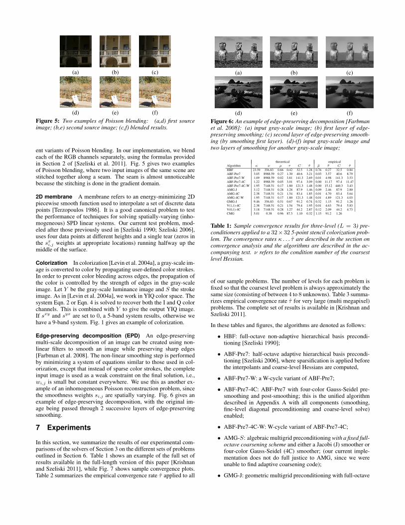
Edge-preserving decomposition (EPD) An edge-preservingmulti-scale decomposition of an image can be created using non-linear filters to smooth an image while preserving sharp edges[Farbman et al. 2008]. The non-linear smoothing step is performedby minimizing a system of equations similar to those used in col-orization, except that instead of sparse color strokes, the completeinput image is used as a weak constraint on the final solution, i.e.,wi,j is small but constant everywhere. We use this as another ex-ample of an inhomogeneous Poisson reconstruction problem, sincethe smoothness weights si,j are spatially varying. Fig. 6 gives anexample of edge-preserving decomposition, with the original im-age being passed through 2 successive layers of edge-preservingsmoothing.

7 Experiments

In this section, we summarize the results of our experimental com-parisons of the solvers of Section 3 on the different sets of problemsoutlined in Section 6. Table 1 shows an example of the full set ofresults available in the full-length version of this paper [Krishnanand Szeliski 2011], while Fig. 7 shows sample convergence plots.Table 2 summarizes the empirical convergence rate τ applied to all

(a) (b) (c)

(d) (e) (f)Figure 6: An example of edge-preserving decomposition [Farbmanet al. 2008]: (a) input gray-scale image; (b) first layer of edge-preserving smoothing; (c) second layer of edge-preserving smooth-ing (by smoothing first layer). (d)-(f) input gray-scale image andtwo layers of smoothing for another gray-scale image;

theoretical empiricalAlgorithm κ ν ρ τ C τ ρ τ C τ

HBF 23.59 356.83 0.66 0.42 32.5 1.28 0.76 0.27 32.5 0.84ABF-Pre7 3.05 8988.59 0.27 1.30 40.6 3.21 0.03 3.57 40.6 8.79ABF-Pre7-W 1.09 8988.59 0.02 3.81 141.3 2.69 0.01 4.98 141.3 3.53ABF-Pre7-4C 1.22 8988.59 0.05 3.01 97.4 3.09 0.00 11.17 97.4 11.47ABF-Pre7-4C-W 1.95 7148.51 0.17 1.80 121.3 1.48 0.00 15.12 440.3 3.43AMG-J 3.12 7148.51 0.28 1.28 87.9 1.46 0.09 2.46 87.9 2.80AMG-4C 2.38 7148.51 0.21 1.54 83.4 1.85 0.01 4.70 83.4 5.64AMG-4C-W 1.95 7148.51 0.17 1.80 121.3 1.48 0.01 4.89 121.3 4.03GMG-J 9.46 356.83 0.51 0.67 91.2 0.74 0.32 1.15 91.2 1.26V(1,1)-4C 2.38 7148.51 0.21 1.54 79.4 1.95 0.01 4.63 79.4 5.83V(0,1)-4C 3.18 7148.51 0.28 1.27 44.2 2.87 0.12 2.09 44.2 4.73CMG 5.01 0.38 0.96 87.3 1.10 0.32 1.15 91.2 1.26

Table 1: Sample convergence results for three-level (L = 3) pre-conditioners applied to a 32×32 5-point stencil colorization prob-lem. The convergence rates κ . . . τ are described in the section onconvergence analysis and the algorithms are described in the ac-companying text. ν refers to the condition number of the coarsestlevel Hessian.

of our sample problems. The number of levels for each problem isfixed so that the coarsest level problem is always approximately thesame size (consisting of between 4 to 8 unknowns). Table 3 summa-rizes empirical convergence rate τ for very large (multi megapixel)problems. The complete set of results is available in [Krishnan andSzeliski 2011].

In these tables and figures, the algorithms are denoted as follows:

• HBF: full-octave non-adaptive hierarchical basis precondi-tioning [Szeliski 1990];

• ABF-Pre7: half-octave adaptive hierarchical basis precondi-tioning [Szeliski 2006], where sparsification is applied beforethe interpolants and coarse-level Hessians are computed,

• ABF-Pre7-W: a W-cycle variant of ABF-Pre7;

• ABF-Pre7-4C: ABF-Pre7 with four-color Gauss-Seidel pre-smoothing and post-smoothing; this is the unified algorithmdescribed in Appendix A with all components (smoothing,fine-level diagonal preconditioning and coarse-level solve)enabled;

• ABF-Pre7-4C-W: W-cycle variant of ABF-Pre7-4C;

• AMG-S: algebraic multigrid preconditioning with a fixed full-octave coarsening scheme and either a Jacobi (J) smoother orfour-color Gauss-Seidel (4C) smoother; (our current imple-mentation does not do full justice to AMG, since we wereunable to find adaptive coarsening code);

• GMG-J: geometric multigrid preconditioning with full-octave

HDR Poisson Membrane Color. 5-pt Color. 9-pt EPD33 512 768 33 128 512 33 256 32 256 239 32 256 239 33 800 535(4) (8) (7) (4) (6) (7) (4) (7) (4) (7) (6) (4) (7) (6) (4) (8) (7)

HBF 3.35 2.09 2.78 3.54 2.80 2.41 0.94 0.7 0.92 1.18 0.93 0.96 1.06 0.82 1.97 1.78 1.37ABF-Pre7 5.42 2.81 2.88 5.39 4.48 4.83 6.41 5.19 8.75 9.97 5.65 4.55 4.17 3.68 3.82 3.09 2.54ABF-Pre7-W 3.15 2.42 2.56 3.41 2.86 2.42 3.98 3.15 2.72 3.43 0.39 1.22 0.65 0.43 0.57 0.25 0.26ABF-Pre7-4C 7.15 5.55 4.75 8.01 7.77 8.49 4.64 4.29 11.29 5.90 3.28 2.65 2.85 2.18 4.03 2.23 1.93ABF-Pre7-4C-W 2.55 1.69 1.91 2.41 1.80 1.74 1.44 0.77 2.51 1.03 0.88 0.71 0.44 0.39 1.14 0.14 0.15AMG-J 4.37 3.20 3.73 4.82 4.40 4.46 3.99 3.32 2.77 2.23 1.10 3.13 1.83 1.07 1.47 0.93 0.72AMG-4C 7.53 4.56 4.95 8.25 6.73 7.21 5.35 4.29 5.58 3.30 1.68 4.02 2.75 1.17 1.91 1.19 0.92AMG-4C-W 4.66 5.32 5.16 5.21 5.25 5.19 3.94 3.30 3.74 2.95 1.81 3.34 2.68 1.70 1.57 1.28 1.16GMG-J 4.65 3.48 4.17 5.09 4.41 4.41 1.06 0.33 1.39 1.14 0.78 1.87 1.21 0.83 0.99 0.89 0.71V(1,1)-4C 6.95 4.59 4.93 7.67 5.03 6.34 2.93 3.68 5.76 2.93 1.43 3.97 2.22 1.00 0.93 0.82 0.39V(0,1)-4C 4.74 2.74 4.28 6.30 3.96 5.36 5.49 5.12 4.68 3.66 2.52 5.09 2.76 1.55 1.48 1.35 0.62CMG 1.36 1.16 1.25 1.92 1.87 2.18 1.82 1.97 - 2.82 2.39 1.56 1.81 1.89 4.87 4.44 4.24

Table 2: Empirical effective convergence rates τ for preconditioners applied to all of our sample problems. The boldface numbers are the“winners” (fastest empirical convergence rate) in each column. For each problem, test results on two image sets and a small version of oneof the sets are provided. The number of rows in the tested image is at the top of each column. Below that is the number of levels is given inparentheses.

HDR Poisson Membrane Color. 5-pt Color. 9-pt EPD2048 × 1365 2048 × 2048 2048 × 2048 1854 × 2048 1854 × 2048 1365 × 2048

(10) (10) (10) (8) (8) (8)

HBF 2.23 2.58 0.96 0.41 0.56 1.65ABF-Pre7 2.61 5.52 3.97 20.35 16.48 2.60ABF-Pre7-4C 5.75 9.52 3.00 12.17 7.56 1.74AMG-J 2.93 5.15 3.35 3.00 2.71 0.60AMG-4C 4.16 7.69 3.33 8.62 4.16 0.87GMG-J 3.21 4.98 0.57 1.05 0.98 0.91V(1,1)-4C 4.06 6.72 3.45 8.94 4.29 0.37V(0,1)-4C 3.55 5.48 4.02 1.41 2.42 0.59CMG - 2.29 1.75 5.58 3.55 4.18

Table 3: Empirical effective convergence rates τ for preconditioners applied to all of our sample problems for multi-megapixel images. Nextto problem size, the number of levels is given in parentheses. The boldface numbers are the “winners” (fastest empirical convergence rate)in each column. The size of the tested image is at the top of each column. Below that is the number of levels in parentheses.

bilinear interpolants and Jacobi smoothing;

• V(m,n)-4C: V-cycle multigrid with a fixed step size and four-color Gauss-Seidel m pre-smoothing and n post-smoothingsteps; the interpolants and Hessians are computed using thesame logic as for AMG-S; this variant tests the effectivenessof using stand-along multigrid cycles instead of PCG;

• CMG: combinatorial multigrid, using the code provided bythe authors of [Koutis et al. 2009].

There are other possible variants such as the original ABF 5-bandedsparsification algorithm from [Szeliski 2006]. The new partial spar-sification we introduce always works better than the original spar-sification both empirically and theoretically, so we do not includethese runs in our results.

Looking at the complete set of results available in the supplemen-tary materials [Krishnan and Szeliski 2011], we see that the relativebehavior of the various algorithms depends both on the amount ofsmoothness and the amount of inhomogeneity in the sample prob-lems, i.e., how regular they are.

HDR and Poisson blending are homogeneous problems, ideallysuited to geometric multigrid. Indeed GMG (and AMG, which re-verts to GMG on uniform problems) have very fast convergence rateτ . Furthermore, τ is independent of the number of levels, as is pre-dicted by multigrid theory. However, when we factor in the compu-tational cost C, the effective convergence rate τ for the ABF-Pre7-4C is significantly better. Using the new partial (7-point stencil)sparsification rule consistently lowers the condition numbers andusually helps the empirical performance. Comparing the empiricalrates for AMG-J and AMG-4C shows that the four-color smootheris a much better choice than Jacobi smoothing for all problems, buthas an especially dramatic effect for the homogeneous problems.

The 2D membrane exhibits a moderate amount of inhomogene-ity, including scattered data constraints and a strong discontinuity.Here, non-adaptive techniques such as HBF and GMG-J start to fallapart. ABF-Pre7 starts to pull away, with the additional smoothing

of ABF-Pre7-4C not providing significant improvement. AMG-4Cis still competitive if we ignore computational costs. CMG, eventhough it’s designed for irregular problems, has slower convergencebecause it uses a piecewise-constant interpolator for what is essen-tially a mostly smooth problem.

The results on colorization (for both 5-point and 9-point fine-levelstencil formulations) are similar to the 2D membrane, even thoughthe number of discontinuities is quite a bit larger. Here, we wouldexpect a full (adaptive coarsening) implementation of AMG-4C todo better, but we currently don’t have such an implementation totest. In terms of theoretical effective convergence rates, CMG isstarting to look competitive, but still doesn’t do as well empirically.

The edge-preserving decomposition is much more challenging. Be-cause of the large number of discontinuities and thinner elongatedstructures, CMG starts to perform very well, both in terms of the-oretical condition numbers, and in terms of practical convergencerates. It will be interesting to compare its performance against true(adaptive coarsening) algebraic multigrid, and also to future ex-tensions of our sparsifying approach that use adaptive coarseningschemes.

Note that for these problems, the theoretical convergence rates pre-dicted by condition number analysis are much worse than the actualempirical convergence rates we observe. We believe the reason forthis is the clustering of eigenvalues after preconditioning, whereasthe theoretical condition number is computed using the largest andsmallest eigenvalues, which may be outliers.

The unified algorithm ABF-Pre7-4C performs well on all the prob-lems, even after taking into account computational load. Furtherresearch into combining adaptive coarsening with the unified algo-rithm may result in better performance for the less smooth problemssuch as edge-preserving decomposition.

0 50 100 150 200 250 300 350 400 450 500−25

−20

−15

−10

−5

0Colorization−2 Levels = 3

Cumulative Flop Count

Err

or (

log)

HBFABF−Pre7ABF−Pre7−4CAMG−JAMG−4CGMG−JV(1,1)−4CV(0,1)−4CCMGABF−Pre7−WABF−Pre7−4C−WAMG−4C−W

0 50 100 150 200 250 300 350 400 450 500−25

−20

−15

−10

−5

0Colorization−2 Levels = 3

Cumulative Flop Count

A−

Err

or (

log)

HBFABF−Pre7ABF−Pre7−4CAMG−JAMG−4CGMG−JV(1,1)−4CV(0,1)−4CCMGABF−Pre7−WABF−Pre7−4C−WAMG−4C−W

Figure 7: Sample convergence plot for three-level (L = 3) precon-ditioners applied to a 32× 32 5-point stencil colorization problem.Top: The horizontal axis plots the number of floating point oper-ations (flops) performed per input (fine-level) variable, while thevertical axis plots the log error between the current and optimalsolutions; Bottom: plot of flops against A-norm of error (defined aseTAe where e is error and A is the Hessian).

8 Discussion and ConclusionsOur experimental results demonstrate that with our new extensionto partial sparsification, adaptive hierarchical basis function precon-ditioning (ABF) outperforms traditional multigrid techniques on awide range of computer graphics and computational photographyproblems. This runs contrary to the usual belief in the multigridcommunity that appropriate smoothing between level transfers isnecessary for reasonable performance. Traditional adaptive hierar-chical basis functions achieve slower (but still reasonable) conver-gence rates without using any smoothing steps, but use many fewercomputations per level because they do not require any smoothing(other than that implicit in the recomputation of the residual at thebeginning of each iteration).

For irregular problems, such as edge-preserving decomposition,adaptive coarsening schemes such as combinatorial and (adaptive)algebraic multigrid start to become important. Our experimentsalso show that taking into account only the number of iterationswithout incorporating flop counts gives a misleading picture of rel-ative performance. However, we note that flop counts are them-selves not a complete predictor of actual performance, since issuessuch as caching and memory access patterns will be important in

high-performance implementations of these algorithms.

Recently, a number of fast edge-aware smoothing techniques havebeen developed for solving tone mapping and colorization problems[Fattal 2009; Gastal and Oliveira 2011]. These techniques havelinear complexity in the number of pixels and have extremely fastcomputational performance. However, the best-performing precon-ditioning methods in our paper also converge in a single iterationfor tone mapping and colorization. Therefore the effective time forprocessing is the multilevel pyramid setup time and a single itera-tion of (preconditioned) conjugate gradient. Both these steps are asmall constant multiple of the number of pixels in the image and arehighly parallel operations. This leads us to believe that a carefullyoptimized GPU version of our MATLAB code would give very fastcomputational performance as well for the tone mapping and col-orization algorithms.

For the other algorithms such as Poisson blending and edge-preserving decomposition, solving a large linear system is a ne-cessity. Our MATLAB code has been written explicitly with GPUimplementation in mind, since such an implementation would beof significant practical interest to the graphics and computer visioncommunities.

Currently, our adaptive hierarchical bases are defined on a fixedhalf-octave grid. However, we believe that the coarsening heuristicsused in AMG could be adapted to our bases. The sparsification stepused in constructing the adaptive interpolants requires a decomposi-tion into coarse and fine variables, where the connections betweenfine variables (which need to be sparsified) are no stronger thanthose to their corresponding coarse-level “parents”. AMG coarsen-ing strategies perform a very similar selection of nodes.

Another promising direction for future research is the extension tothree-dimensional and more unstructured meshes. The advancesavailable by combining all of these ideas together should lead toeven more efficient techniques for the solution of large-scale two-and three-dimensional computer graphics and computational pho-tography problems.

References

AGARWALA, A., ET AL. 2004. Interactive digital photomontage.ACM Transactions on Graphics (Proc. SIGGRAPH 2004) 23, 3(August), 292–300.

AGARWALA, A. 2007. Efficient gradient-domain compositingusing quadtrees. ACM Transactions on Graphics (Proc. SIG-GRAPH 2007) 26, 3 (August), 94:1–94:5.

BRIGGS, W. L., HENSON, V. E., AND MCCORMICK, S. F. 2000.A Multigrid Tutorial, second ed. Society for Industrial and Ap-plied Mathematics, Philadelphia.

DAVIS, T. A. 2006. Direct Methods for Sparse Linear Systems.SIAM.

FARBMAN, Z., FATTAL, R., LISCHINSKI, D., AND SZELISKI, R.2008. Edge-preserving decompositions for multi-scale tone anddetail manipulation. ACM Transactions on Graphics (Proc. SIG-GRAPH 2008) 27, 3 (August).

FARBMAN, Z., HOFFER, G., LIPMAN, Y., COHEN-OR, D., ANDLISCHINSKI, D. 2009. Coordinates for instant image cloning.ACM Transactions on Graphics (Proc. SIGGRAPH 2009) 28, 3(August).

FATTAL, R., LISCHINSKI, D., AND WERMAN, M. 2002. Gradientdomain high dynamic range compression. ACM Transactions onGraphics 21, 3 (July), 249–256.

FATTAL, R. 2009. Edge-avoiding wavelets and their applications.ACM Transactions on Graphics (Proc. SIGGRAPH 2009) 28, 3(August).

GASTAL, E. S. L., AND OLIVEIRA, M. M. 2011. Domain trans-form for edge-aware image and video processing. ACM Trans-actions on Graphics (Proc. SIGGRAPH 2011) 30, 4 (July).

GORTLER, S. J., AND COHEN, M. F. 1995. Hierarchical andvariational geometric modeling with wavelets. In Symposium onInteractive 3D Graphics, 35–43.

JESCHKE, S., CLINE, D., AND WONKA, P. 2009. A GPU Lapla-cian solver for diffusion curves and Poisson image editing. ACMTransactions on Graphics (Proc. SIGGRAPH Asia 2009) 28, 5(December).

KAZHDAN, M., SURENDRAN, D., AND HOPPE, H. 2010. Dis-tributed gradient-domain processing of planar and spherical im-ages. ACM Transactions on Graphics 29, 2 (April).

KOUTIS, I., MILLER, G. L., AND TOLLIVER, D. 2009. Com-binatorial preconditioners and multilevel solvers for problems incomputer vision and image processing. In 5th International Sym-posium on Visual Computing (ISVC09), Springer.

KRISHNAN, D., AND SZELISKI, R. 2011. Multigrid and multi-level preconditioners for computational photography. Tech. Rep.NYU-TR-941, New York University, October.

KUSHNIR, D., GALUN, M., AND BRANDT, A. 2010. Efficientmultilevel eigensolvers with applications to data analysis tasks.IEEE Transactions on Pattern Analysis and Machine Intelligence32, 8 (August), 1377–1391.

LEVIN, A., LISCHINSKI, D., AND WEISS, Y. 2004. Coloriza-tion using optimization. ACM Transactions on Graphics 23, 3(August), 689–694.

LEVIN, A., ZOMET, A., PELEG, S., AND WEISS, Y. 2004. Seam-less image stitching in the gradient domain. In Eighth EuropeanConference on Computer Vision (ECCV 2004), Springer-Verlag,vol. IV, 377–389.

LEVIN, A., LISCHINSKI, D., AND WEISS, Y. 2008. A closed-form solution to natural image matting. IEEE Trans. on PatternAnalysis and Machine Intelligence 30, 2 (Feb.), 228–242.

MCADAMS, A., SIFAKIS, E., AND TERAN, J. 2010. A paral-lel multigrid Poisson solver for fluids simulation on large grids.ACM SIGGRAPH/Eurographics Symposium on Computer Ani-mation, 65–74.

MCCANN, J., AND POLLARD, N. 2008. Real-time gradientdomain painting. ACM Transactions on Graphics (Proc. SIG-GRAPH 2008) 27, 3 (August).

NAPOV, A., AND NOTAY, Y. 2011. Algebraic analysis ofaggregation-based multigrid. Numerical Linear Algebra withApplications 18, 3 (May), 539–564.

PENTLAND, A. P. 1994. Interpolation using wavelet bases. IEEETransactions on Pattern Analysis and Machine Intelligence 16,4 (April), 410–414.

PEREZ, P., GANGNET, M., AND BLAKE, A. 2003. Poisson im-age editing. ACM Transactions on Graphics (Proc. SIGGRAPH2003) 22, 3 (July), 313–318.

ROBERTS, A. 2001. Simple and fast multigrid solutions of Pois-son’s equation using diagonally oriented grids. ANZIAM J. 43(July), E1–E36.

SAAD, Y. 2003. Iterative Methods for Sparse Linear Systems,second ed. Society for Industrial and Applied Mathematics.

SHEWCHUK, J. R. 1994. An introduction to the conjugate gra-dient method without the agonizing pain. http://www.cs.berkeley.edu/˜jrs/, August.

SZELISKI, R., UYTTENDAELE, M., AND STEEDLY, D. 2011. FastPoisson blending using multi-splines. In International Confer-ence on Computational Photography (ICCP 11).

SZELISKI, R. 1990. Fast surface interpolation using hierarchicalbasis functions. IEEE Transactions on Pattern Analysis and Ma-chine Intelligence 12, 6 (June), 513–528.

SZELISKI, R. 2006. Locally adapted hierarchical basis precon-ditioning. ACM Transactions on Graphics (Proc. SIGGRAPH2006) 25, 3 (August), 1135–1143.

TERZOPOULOS, D. 1986. Image analysis using multigrid relax-ation methods. IEEE Transactions on Pattern Analysis and Ma-chine Intelligence PAMI-8, 2 (March), 129–139.

TROTTENBERG, U., OOSTERLEE, C. W., AND SCHULLER, A.2000. Multigrid. Academic Press.

WANG, H., RASKAR, R., AND AHUJA, N. 2004. Seamless videoediting. Proceedings of the International Conference on PatternRecognition, 858–861.

A Unified multilevel multigrid preconditioner

Algorithm 1 Unified multigrid/multilevel algorithm[el] = MGCYC(l, rl, A1 . . . AL, S1 . . . SL,MG)INPUT: Current level l, residual rl , per-level HessiansAl ,per-level interpolation matrices Sl ,MG is a parameter structure that contains:number of levelsMG.L, damping factorMG.ω,pre- and post-smoothing iterationsMG.νpre

andMG.νpost , number of cyclesMG.γ,flag for optional diagonal preconditioningMG.dOUTPUT: Correction at level l el

1. // Pre-smoothing correctioneprel

= Smooth (0, Al, rl, ω, νpre)

2. // Update the residualrl = rl − Ale

prel

3. // Restrict residual to coarse levelrl+1 = STl rl

4. if l = L − 1

5. el+1 = A−1L

rl+16. else7. el+1 = 0

8. //γ = 1 is V-cycle; γ = 2 is W-cyclefor j = 1, . . . γ

9. // Update the residualrl+1 = rl+1 − Al+1el+1

10. el+1 = MGCYC(l + 1, rl+1, A1 . . . AL,S1 . . . SL,MG)

11. // Add up corrections over the cyclesel+1 ← el+1 + el+1

12. endfor13. endif14. // Prolong coarse-grid correction

ecgcl

= Slel+115. // Optional fine-level diagonal preconditioning

if (d = 1)16. // Precondition with inverse diagonal elements ofAl .

edl = DiagPrecond(rl ,Al )17. else18. // No diagonal preconditioning

edl = 019. endif20. // Add up corrections: pre-smooth, coarse-level, and diagonal

esuml = eprel

+ ecgcl

+ edl21. // Post-smoothing

el = Smooth(esuml ,Al, rl, ω, νpost)