www.oeaw.ac.at

www.ricam.oeaw.ac.at

Overlapping Additive Schwarzpreconditioners for

degenerated elliptic problems:Part I- isotropic problems

S. Beuchler, S.V. Nepomnyaschikh

RICAM-Report 2006-32

Overlapping Additive Schwarz preconditioners fordegenerated elliptic problems: Part I isotropic problems

Sven BeuchlerInstitute for Computational Mathematics

University of LinzAltenberger Strasse 69A-4040 Linz, Austria

sven.beuchler@jku.at

Sergey V. NepomnyaschikhInstitute for Computational Mathematics

and Computational GeophysicsSD Russian Academy of Sciences

Novosibirsk, Russiasvnep@oapmg.sscc.ru

November 8, 2006

Abstract

In this paper, we consider the degenerated isotropic boundary value problem−∇(ω2(x)∇u(x, y)) =f(x, y) on the unit square(0, 1)2. The weight function is assumed to be of the formω2(ξ) = ξα, whereα ≥ 0. This problem is discretized by piecewise linear finite elements on a triangular mesh of isoscelesright-angled triangles. The system of linear algebraic equations is solved by a preconditioned gradientmethod using a domain decomposition preconditioner with overlap. Two different preconditioners arepresented and the optimality of the condition number for the preconditioned system is proved forα 6= 1.The preoconditioning operation requiresO(N) operations, whereN is the number of unknowns. Severalnumerical experiments show the preformance of the proposed method.

1 Introduction

In this paper, we investigate the degenerated and isotropic boundary value problem

−(ω2(x)ux)x − (ω2(x)uy)y = f, in Ω = (0, 1)2

u = 0, on ∂Ω (1.1)

with some strongly monotonic increasing and bounded weight functionω : [0, 1] 7→ R satisfyingω(0) = 0.In the past, degenerated problems have been considered relatively rarely. One reason is the unphysicalbehavior of the partial differential equation (pde) which is quite unusual in technical applications. Onework focusing on this type of partial differential equation is the book of Kufner and Sandig [17]. Nowa-days, problems of this type become more and more popular because there are stochastic pde’s of a similarstructure. An example of an isotropic degenerated stochastic pde is the Black-Scholes pde, [21].

1

Moreover, there are examples of locally anisotropic degenerated elliptic problems. One of them is the solverrelated to the problem of the sub-domains for thep-version of the finite element method using quadrilateralelements. This matrix can be interpreted ash-version fem-discretization matrix of the problem−y2uxx −x2uyy = f . We refer to [1], [2] for more details.The discretization of (1.1) using theh-version of the finite element method (fem) leads to a linear systemof algebraic equations

Ku = f. (1.2)

It is well known from the literature that preconditioned conjugate gradient-methods (pcg-methods) withdomain decomposition preconditioners are among the most efficient iterative solvers for systems of thetype (1.2), see e.g. [7], [8], [9], [10], [23], [18]. In this paper, we will propose and analyze overlappingDomain Decomposition (DD) preconditioners.The type of overlapping DD-preconditioners presented in this paper is originally developed for problemswith jumping coefficients in [20], see also [13], [22] for the case of highly variying coefficients. In a sec-ond paper [3], we will analyze these overlappingDD preconditioners for a locally anisotropic degeneratedproblems. Here, we adapt the techniques of [20] to problem (1.1). To keep the notation and the proofs sim-ple, we will prove the optimality of this method only for tensor product discretizations in two dimensions.The generalization of the method to three dimensional tensor product discretizations is straightforward.Moreover, this method can be extended to more generalh-version fem discretizations, using the ficticousspace lemma, [19].Only a limited number of papers have investigated fast solvers for degenerated elliptic problems. The paper[6] deals with the Laplacian in2D in polar coordinates. In the paper [12], multigrid methods for someother types of degenerated problems are proposed. Multigrid solvers for FE-discretizations of the problemsin [3] have been investigated in [1], see also [5] and [16]. The paper [4] proposes wavelet methods forseveral classes of degenerated elliptic problems on the unit square. One of them is problem (1.1) under the

restriction limξ→0+

ξ

ω2(ξ)= 0 to the weight functions. Moreover, a fast direct solver based on eigenvalue

computations combined with fast Fourier transform can be designed if a tensor product discretization isused.The remaining part of this paper is organized as follows. In Section 2, we introduce the reader into ourproblem and into our notation. The preconditioners are defined in Section 3. Moreover, the main theoremswith the condition number estimates are stated. The efficient solution of the preconditioned systems willbe presented in Section 4. In Section 5, we formulate some auxiliary results from the Additive SchwarzMethod (ASM), which are required for the proofs of our main theorems given in Section 6. In Section 7, wepresent some numerical experiments which show the performance of the presented methods. Finally, wepresent some concluding remarks and generalizations to a general domain using the Ficticous space lemma.Throughout this paper, the integerk denotes the level number. For two real symmetric and positive definiten × n matricesA,B, the relationA B means thatA − cB is negative definite, wherec > 0 is aconstant independent ofn. The relationA ∼ B meansA B andB A, i.e. the matricesA andB arespectrally equivalent. The parameterc denotes a generic constant. The isomorphism between a functionu =

∑i uiψi ∈ L2 and the corresponding vector of coefficientsu = [ui]i in the basis[Ψ] = [ψ1, ψ2, . . .] is

denoted byu = [Ψ]u.

2 Setting of the problem

In this paper, we investigate the following boundary value problem: LetΩ = (0, 1)2. Findu ∈ Hω,0 :=u ∈ L2(Ω) :

∫Ωω2(x)(∇u)T∇u d(x, y) <∞, u |∂Ω= 0 such that

a(u, v) :=∫

Ω

ω2(x)(∇v)T (x, y)∇u(x, y) d(x, y) = (f, v) ∀v ∈ Hω,0. (2.1)

2

We point out that the diffusion matrixD = ω2(x)I of (2.1), whereI denoted the unity matrix, is notnecessarily uniformly positive definite inΩ.To be specific, we consider the weight functionω2(x) = xα, α > 0.

Lemma 2.1. The functionω : [0, 1] 7→ R given byω2(x) = xα, α > 0 satisfies the following assertions:

• the functionω is monotonic increasing,

• the functionω is continuous,

• the estimate

ω(2ξ) ≤ cωω(ξ) ∀ξ ∈(

0,12

](2.2)

holds with some constantcω = 2−α/2 > 0.

Problems of the type (2.1) are called degenerated problems. In the past, degenerated problems have beenconsidered relatively rarely. One reason is the unphysical behavior of the partial differential equation whichis quite unusual in technical applications. Nowadays, problems of this type become more and more popularbecause there are stochastic pde’s which have a similar structure. Settingω(ξ) = ξ, one obtains a degener-ated stochastic partial differential equation, i.e. the Black-Scholes partial differential equation, [21].We discretize problem (2.1) by piecewise linear finite elements on the regular Cartesian grid consisting ofcongruent, isosceles, right-angled triangles. For this purpose, some notation is introduced. Letk be thelevel of approximation andn = 2k. Let xk

ij = ( in ,

jn ), wherei, j = 0, . . . , n. The domainΩ is divided

into congruent, isosceles, right-angled trianglesτ s,kij , where0 ≤ i, j < n ands = 1, 2, see Figure 1. The

triangleτ1,kij has the three verticesxk

ij , xki+1,j+1 andxk

i,j+1, τ2,kij has the three verticesxk

ij , xki+1,j+1 and

xki+1,j , see Figure 1. Piecewise linear finite elements are used on the meshTk = τ s,k

ij n−1,n−1,2i=0,j=0,s=1. The

6

-

(0, 0) (1, 0)

(0, 1)

xkij

xki,j+1

xki+1,j

xki+1,j+1

τ1,kij

τ2,kij

Figure 1: Mesh for the finite element method (left), Notation within a macro-elementEkij (right).

subspace of piecewise linear functionsφkij with

φkij ∈ H1

0 (Ω), φkij |τs,k

lm∈ P1(τ

s,klm )

is denoted byVk, whereP1 is the space of polynomials of degree≤ 1. A basis ofVk is the system of theusual hat-functionsΦk = φk

ijn−1i,j=1 uniquely defined by

φkij(x

klm) = δilδjm

3

andφkij ∈ Vk, whereδil is the Kronecker delta. Now, we can formulate the discretized problem.

Finduk ∈ Vk such thata(uk, vk) = (f, vk) ∀vk ∈ Vk (2.3)

holds. Problem (2.3) is equivalent to solving the system of linear algebraic equations

Kkuk = fk, (2.4)

whereKk =[a(φk

ij , φklm)

]n−1

i,j,l,m=1, uk = [uij ]

n−1i,j=1 andf

k=

[(f, φk

lm)〉]n−1

l,m=1. The size of the matrix

Kk isN ×N with N = (n− 1)2.

3 Definition of the preconditioners

In this section, we define the preconditioners for the matrixKk (2.3). We introduce the following notation.Let

• Ωi,x =(x, y) ∈ R2, 2−1−i < x < 2−i, 0 < y < 1

, i = 0, . . . , k − 2,

• Ωk−1,x =(x, y) ∈ R2, 0 < x < 2−k, 0 < y < 1

,

• Γi,x =(x, y) ∈ R2, x = 2−i, 0 < y < 1

, i = 1, . . . , k − 1,

• Ωj,x = int(⋃k−1

i=j Ωi,x

), and

• nj = 2k−j − 1 be the number of interior grid points inΩj,x in x-direction andNj = (n − 1)nj bethe total number of interior grid points.

• Moreover, letεj = ω2

(2−j

).

Figure 2 displays a sketch with the notation in the casek = 4. On Ωj,x, we introduce the bilinear form

ΩΩΩ 0,xΩ1,x2,x3,x Ω1,x

~

Γ1,xΓ2,x3,xΓ

Figure 2: Notation fork = 4.

aj(u, v) =∫

Ωj,x

∇u · ∇v, j = 0, . . . , k − 1.

4

Moreover, let

Cj,D = [aj(φii′ , φll′)]nj ,n0i,l=1; i′,l′=1 , j = 0, . . . , k − 1, and

Cj,N = [aj(φii′ , φll′)]nj ,n0i,l=nj+1+1;i′,l′=1 , j = 0, . . . , k − 2.

These matrices correspond to the Laplacian onΩj,x with Dirchlet boundary conditions at the left boundaryx = 0 and to the Laplacian onΩj,x with Neumann boundary conditions at the left boundaryΓj+1,x. At theremaining three edges, we have Dirichlet boundary conditions. Finally, let

∆j,D =[Cj,D 00 0N−Nj

]∈ RN×N and ∆j,N =

0Nj+1 0 00 Cj,N 00 0 0N−Nj

∈ RN×N (3.1)

be the global assembled stiffness matrices.Then, we define a first preconditioner

C−1 =k−1∑j=0

ε−1j ∆+

j,D, (3.2)

whereB+ denotes the pseudo-inverse inverse of a matrixB. Then, we can prove the following result.

Theorem 3.1. Let C be defined via(3.2) and letω2(ξ) = ξα. If α > 0, then we haveKk C. If0 ≤ α < 1

2 , then we have alsoC Kk.

Proof. A detailed proof is presented in subsection 6.4.

Since Theorem 3.1 can be proved only forα < 12 directly, we introduce a second preconditioner. Let

Cj,D =

[∫Ωj,x∪Ωj+1,x

∇φii′ · ∇φll′

]nj ,n0

i,j=nj+2+2; i′,l′=1

be the Laplacian onΩj+1,x ∪ Ωj,x with Dirichlet boundary conditions at all edges and

∆j,D =

0Nj+2+n0 0 00 Cj,D 00 0 0N−Nj

∈ RN×N , j = 0, . . . , k − 2, (3.3)

be the corresponding assembled matrix. Then, we introduce a second overlapping preconditioner forKk as

C−1mod =

k−2∑j=0

ε−1j ∆+

j,D + ε−1k−1∆

+k−1,D. (3.4)

Theorem 3.2. Let Cmod be defined via(3.4). Let ω2(ξ) = ξα with α 6= 1. Then, the matrixCmod issymmetric positive definite and satisfiesKk ∼ Cmod.

Proof. A detailed proof is given in subsection 6.1 forα > 1 and in subsection 6.2 forα < 1.

Remark 3.3. From the definition of the preconditioners, the relationCmod ≤ C follows directly. Combin-ing Theorem 3.1 and Theorem 3.2, the estimateC ∼ Kk holds ifα 6= 1 andα > 0. In the caseα = 1, weare not able to prove an optimal result. Here, only the weaker estimatek−2C Kk C can be proved.This behavior can also be seen in the numerical experiments of section 7.

5

4 Computational aspects

In this section, we investigate the preconditioning operationC−1w for the two preconditioners of pro-ceeding section. We present algorithms to perform this preconditioning operation in optimal arithmeticalcomplexity.We have developed the preconditioners

C−1 =k−1∑j=0

ε−1j ∆+

j,D,

see (3.2) and

C−1mod =

k−2∑j=0

ε−1j ∆+

j,D + ε−1k−1∆

+k−1,D,

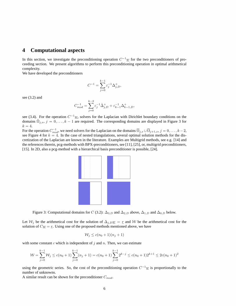
see (3.4). For the operationC−1w, solvers for the Laplacian with Dirichlet boundary conditions on thedomainsΩj,x, j = 0, . . . , k − 1 are required. The corresponding domains are displayed in Figure 3 fork = 4.For the operationC−1

mod, we need solvers for the Laplacian on the domainsΩj,x∪Ωj+1,x, j = 0, . . . , k−2,see Figure 4 fork = 4. In the case of nested triangulations, several optimal solution methods for the dis-cretization of the Laplacian are known in the literature. Examples are Multigrid methods, see e.g. [14] andthe references therein, pcg-methods with BPX-preconditioners, see [11], [25], or, multigrid preconditioners,[15]. In 2D, also a pcg-method with a hierarchical basis preconditioner is possible, [24].

Figure 3: Computational domains forC (3.2): ∆3,D and∆2,D above,∆1,D and∆0,D below.

Let Wj be the arithmetical cost for the solution of∆j,Dw = r andW be the arithmetical cost for thesolution ofCw = r. Using one of the proposed methods mentioned above, we have

Wj ≤ c(n0 + 1)(nj + 1)

with some constantc which is independent ofj andn. Then, we can estimate

W =k−1∑j=0

Wj ≤ c(n0 + 1)k−1∑j=0

(nj + 1) = c(n0 + 1)k−1∑j=0

2k−j ≤ c(n0 + 1)2k+1 ≤ 2c(n0 + 1)2

using the geometric series. So, the cost of the preconditioning operationC−1w is proportionally to thenumber of unknowns.A similar result can be shown for the preconditionerCmod.

6

Figure 4: Computational domains forCmod (3.4): ˆDelta3,D and∆2,D above,∆1,D and∆0,D below.

5 Preliminaries

In this section, we will formulate some auxiliary results.

5.1 Preliminaries from the Additive Schwarz Method

We start this subsection with the formulation of two results about the additive Schwarz method with inexactsubproblem solvers. These results are developed in [19].

Lemma 5.1. LetH be a Hilbert space with the scalar product(·, ·). Moreover, letHi, i = 1, . . . ,msubspaces ofH such that

H = H1 +H2 + . . .+Hm.

LetA : H 7→ H be a linear, self adjoint, bounded and positive definite operator and let

(u, v)A = (Au, v) ∀u, v ∈ H.

We denote byPi, i = 1, . . . ,m, the orthogonal projection operators fromH ontoHi with respect to thescalar product(·, ·)A. We assume that for anyu ∈ H there exists a decompositionu = u1 + . . .+ um suchthat

c1

m∑i=1

(ui, ui)A ≤ (u, u)A (5.1)

with a positive constantc1. Moreover, letc2 some positive constant such that

m∑i=1

(Piu, u)A ≤ c2 (u, u)A ∀u ∈ H. (5.2)

Also, letBi : H 7→ Hi, i = 1, . . . ,m be some selfadjoint operators such that

c3 (Biui, ui) ≤ (Aui, ui) ≤ c4 (Biui, ui) , ∀ui ∈ Hi, i = 1, . . . ,m. (5.3)

LetB−1 = B+1 + . . .+ B+

m, whereB+i denotes the pseudo-inverse operator forBi. Then,

c1c3(A−1u, u

)≤

(B−1u, u

)≤ c2c4

(A−1u, u

)∀u ∈ H.

7

Lemma 5.2. LetV andW be two Hilbert spaces with scalar products(·, ·)V

and(·, ·)W

. Moreover, letΣandS be selfadjoint, positive definite operators inV andW, respectively. We denote by

(φ, ψ)Σ = (Σφ, ψ)V

and (u, v)S = (Su, v)W

the scalar products inV andW generated by the operatorsΣ andS. LetE : V 7→W be a linear operatorsuch that

α (φ, φ)Σ ≤ (Eφ, Eφ)S ≤ β (φ, φ)Σ ∀φ ∈ V.

Finally, we setC+ = EΣ−1E∗,

whereE∗ is the adjoint to the operator with respect to the scalar products(·, ·)V

and(·, ·)W

. Then,

α (Cu, u)W≤ (Su, u)

W≤ β (Cu, u)

W∀u ∈ Im(E) := u ∈W;∃v ∈ V : u = Ev.

5.2 Algebraic Analysis of an overlapping DD-preconditioner

In this subsection, we prove an auxiliary result for an overlapping domain decomposition preconditioner inwhich the domainΩ is decomposed into stripesΩi. We consider the following situation:

• Let

Ω =k−1⋃j=0

Ωj

be a domainΩ which is decomposed into stripesΩi, i.e.

Ωi ∩ Ωj = ∅ for i 6= j, Ωi ∩ Ωj =

Γi i = j + 1Γj i = j − 1Ωi i = j∅ |i− j| ≥ 2

and letΩk−1 ∩ ∂Ω = Γk.

• Let τk be a triangulation ofΩ which is admissible with the decomposition ofΩ into Ωi.

• Let Φk = [φi]Ni=1 be the basis of hat functions according to the triangulationτk andVk = spanΦk

be the corresponding finite element space.

• Let a(·, ·) : Vk ×Vk 7→ R be a symmetric and positive definite bilinear form and let

‖ u ‖a,Ω= a(u, u)

be the energetic norm. In the same way, let

‖ u ‖a,Ω= a |Ω (u, u)

be the restriction of the norm onto a subdomainΩ ⊂ Ω.

• For j = 0, . . . , k − 2, letYj = u ∈ Vk : supp u ⊂ Ωj ∪ Ωj+1 be the restriction of the finiteelement spaceVk ontoΩj∪Ωj+1 with Dirichlet boundary conditions at the boundariesΓj andΓj+2.For j = k − 1, we setYk−1 = u ∈ Vk : supp u ⊂ Ωk−1.

8

• Let

‖ w ‖2Γj ,left= minu ∈ Vk

u |Γj = wu |Γj+1= 0

‖ u ‖2a,Ωjand ‖ w ‖2Γj ,right= min

u ∈ Vk

u |Γj = wu |Γj−1= 0

‖ u ‖2a,Ωj−1(5.4)

be the left and right trace norm onΓj .

Theorem 5.3. Let all assumptions be satisfied. Then, for all decompositions ofu into uj , the assertion

a(u, u) ≤ 2k−1∑j=0

a(uj , uj) ∀u =k−1∑j=0

uj , whereuj ∈ Yj

holds.

Proof. The proof is simple. Due to the construction of the spacesYj , we have

a(u, v) = 0 ∀u ∈ Yj , v ∈ Yj′ , |j − j′| > 1.

Using the Cauchy inequality and the arithmetical-geometrical mean value, we can conclude that

a(u, u) =k−1∑

j,j′=1

a(uj , uj′) =k−1∑j=0

a(uj , uj) + 2k−2∑j=0

a(uj , uj+1)

≤k−1∑j=0

a(uj , uj) + 2k−2∑j=0

√‖ uj ‖2a,Ωj+1

‖ uj+1 ‖2a,Ωj+1

≤k−1∑j=0

a(uj , uj) +k−2∑j=0

(‖ uj ‖2a,Ωj+1+ ‖ uj+1 ‖2a,Ωj+1

)

≤ 2k−1∑j=0

a(uj , uj).

This proves the assertion.

Theorem 5.4. In addition to the above assumptions, let us assume the following:There exists a integerj0 such that

• There exists a constantγ < 1 which is independent of the discretization parameter andj such that

a(u, v) ≤ γ ‖ u ‖a,Ωj+1‖ v ‖a,Ωj+1 ∀j = 0, . . . , j0, ∀u ∈ Yj ,∀v ∈ Yj+1. (5.5)

• There exists a constantq < 1 and a constantc2 which are independent ofj and the discretizationparameter such that

q−1 ‖ w ‖2Γj ,left≤‖ w ‖2Γj ,right≤ c2 ‖ w ‖2Γj ,left ∀w, j = j0 + 1, . . . , k − 1. (5.6)

• There exists a constantc1 which is independent of discretization parameter such that

c−11 ‖ w ‖2Γj ,left≤‖ w ‖2Γj ,right≤ c2 ‖ w ‖2Γj ,left ∀w, j = j0. (5.7)

9

Then, there exists a decompositionu =∑k−1

j=0 uj with uj ∈ Yj such that

c2L

k−1∑j=0

a(uj , uj) ≤ a(u, u) ∀u ∈ Vk.

The constantcL > 0 depends only onγ, c1, c2 andq.

Proof. We construct an explicit decomposition using extension operatorsTj,left/right and start the proof withthe definition of extension operatorsTj,left. For a given functionw ∈ Vk |Γj

, let Tj,left : Vk |Γj7→ Vk |Ωj

be defined by the following conditions:

Tj,leftw ∈ Vk |Ωj, Tj,leftw |Γj

= w

supp Tj,leftw ⊂ Ωj a(Tj,leftw, v) = 0 ∀v ∈ Vk, supp v ⊂ Ωj . (5.8)

Due to this definition, the operatorTj,left is the discrete energetic extension fromΓj+1 to Ωj+1. Moreover,let Tj,right : Vk |Γj

7→ Vk |Ωj−1 be defined by the following conditions:

Tj,rightw ∈ Vk |Ωj−1, Tj,rightw |Γj = w

supp Tj,rightw ⊂ Ωj−1 a(Tj,rightw, v) = 0 ∀v ∈ Vk, supp v ⊂ Ωj . (5.9)

Due to this definition, the operatorTj,right is the discrete energetic extension fromΓj to Ωj−1.We decompose a givenu ∈ Vk into the functionsuj ∈ Yj into the following way:

u0 =

u in Ω0

T0,leftw1 in Ω1

0 else,

uj =

u− uj−1 in Ωj

Tj,leftwj+1 in Ωj+1

0 else, j = 1, . . . , k − 2, (5.10)

uk−1 =u− uk−2 in Ωk−1

0 else

withwj = u |Γj , j = 1, . . . , k − 1, and wk = 0.

Due to the construction of the functionsuj , the functionuj belongs toYj . We consider now the strength-ened Cauchy inequality between the spacesYj andYj+1, i.e.

γ2j = max

uj ∈ Yj

uj+1 ∈ Yj+1

uj , uj+1 6= 0

a2(uj , uj+1)a(uj , uj)a(uj+1, uj+1)

. (5.11)

We will prove that it is possible to restrict ourselves to the traces of the functionsuj on Γj+1. For a giventrace functionwj , let

gj =

Tj,leftwj in Ωj

Tj,rightwj in Ωj−1

0 else

∈ Yj−1, j = 1, . . . , k,

10

with Tj,right of (5.9). Due to the construction of the functiongj , we can conclude that

‖ gj ‖a,Ωj=‖ wj ‖Γj ,left and ‖ gj ‖a,Ωj−1=‖ wj ‖Γj ,right, j = 1, . . . , k. (5.12)

Moreover,

uj+1 = uj+1,I + gj+2, where

uj+1,I |Γj+2= 0, uj+1 |Γj+2= gj+2, a(gj+2, uj+1,I) = 0, j = 0, . . . , k − 2.

A direct consequence ofa(gj+2, uj+1,I) = 0 and (5.12) is the relation

a(uj+1, uj+1) = a(gj+2, gj+2) + a(uj+1,I , uj+1,I)= ‖ gj+2 ‖2a,Ωj+2

+ ‖ gj+2 ‖2a,Ωj+1+a(uj+1,I , uj+1,I) (5.13)

= ‖ wj+2 ‖2Γj+2,left + ‖ wj+2 ‖2Γj+2,right +a(uj+1,I , uj+1,I), j = 0, . . . , k − 2.

With the same arguments, we obtain

a(uj , uj) = a(gj+1, gj+1) + a(uj,I , uj,I) (5.14)

= ‖ wj+1 ‖2Γj+1,left + ‖ wj+1 ‖2Γj+1,right +a(uj,I , uj,I), j = 0, . . . , k − 1.

Sincea(Tj+1w, uj+1,I) = 0, we can conclude with the strengthened Cauchy inequality and (5.12) that

2|a(uj , uj+1)| = 2∣∣a |Ωj+1 (uj , uj+1)

∣∣ = 2∣∣a |Ωj+1 (Tj+1wj , uj+1)

∣∣= 2

∣∣a |Ωj+1 (gj+1, gj+2 + uj+1,I)∣∣

= 2∣∣a |Ωj+1 (gj+1, gj+2)

∣∣ (5.15)

≤ 2γj ‖ gj+1 ‖a,Ωj+1‖ gj+2 ‖a,Ωj+1

= 2γj

√βj ‖ wj+1 ‖Γj+1,left

√β−1

j ‖ wj+2 ‖Γj+2,right

≤ βjγj ‖ wj+1 ‖2Γj+1,left +β−1j γj ‖ wj+2 ‖2Γj+2,right, j = 0, . . . , k − 2

with some positive parametersβj specified later. The constantγj denotes the constant of strengthenedCauchy inequality, which satisfies the estimateγj ≤ 1, j = 0, . . . , k − 2.We use now the estimates (5.13), (5.14) and (5.15) and can conclude

a(u, u) =k−1∑j=0

a(uj , uj) + 2k−2∑j=0

a(uj , uj+1) (5.16)

≥k−1∑j=0

a(uj,I , uj,I) +k−2∑j=0

‖ wj+1 ‖2Γj+1,left + ‖ wj+1 ‖2Γj+1,right

−

k−2∑j=0

βjγj ‖ wj+1 ‖2Γj+1,left +β−1j γj ‖ wj+2 ‖2Γj+2,right

≥

k−2∑j=0

(1− βjγj) ‖ wj+1 ‖2Γj+1,left +(1− β−1j−1γj−1) ‖ wj+1 ‖2Γj+1,right +

k−1∑j=0

a(uj,I , uj,I).

11

In the above estimate, we have setγ−1 = 0 per definition and usedwk = 0. Let

s0 :=j0−1∑j=0

(1− βjγj) ‖ wj+1 ‖2Γj+1,left +(1− β−1j−1γj−1) ‖ wj+1 ‖2Γj+1,right,

s1 := (1− βj0γj0) ‖ wj0+1 ‖2Γj0+1,left +(1− β−1j0−1γj0−1) ‖ wj0+1 ‖2Γj0+1,right,

s2 :=k−2∑

j=j0+1

(1− βjγj) ‖ wj+1 ‖2Γj+1,left +(1− β−1j−1γj−1) ‖ wj+1 ‖2Γj+1,right . (5.17)

We define now

βj =

1 j ≤ j0 − 1β j ≥ j0

with β = min√

q−1, 1 +1− γ

2c1

.

The assumption (5.5) impliesγj ≤ γ < 1 for j ≤ j0. Hence, we obtain the estimate

s0 ≥ (1− γ)j0−1∑j=0

‖ wj+1 ‖2Γj+1,left + ‖ wj+1 ‖2Γj+1,right . (5.18)

The estimatesq < 1, γ < 1 andc1 > 0 imply β > 1 and

(1− γ) + c1(1− β) ≥ 12(1− γ).

Using assumption (5.7), we can estimate

s1 ≥((1− βj0γj0) + c−1

1 (1− β−1j0−1γj0−1)

)‖ wj0+1 ‖2Γj0+1,left

≥ 1c1

((1− γ) + c1(1− β)) ‖ wj0+1 ‖2Γj0+1,left

≥ 1− γ

2c1‖ wj0+1 ‖2Γj0+1,left≥

1− γ

2c11

1 + c2

(‖ wj0+1 ‖2Γj0+1,left + ‖ wj0+1 ‖2Γj0+1,right

).

Finally, we estimates2. The assumption (5.6),β > 1 andγj ≤ 1 imply

s2 ≥(

1− β + (1− β−1)1q

) k−2∑j=j0+1

‖ wj+1 ‖2Γj+1,left . (5.19)

The estimateβ ≤√q−1 implies 1

q ≥ β2 ≥ 1. Hence, we can estimate(1− β + (1− β−1)

1q

)≥ (1− β) + (1− β−1)β2 = (1− β)2 > 0.

Inserting this estimate into (5.19) and using (5.7) yields

s2 ≥(1− β)2

1 + c2

k−2∑j=j0+1

(‖ wj+1 ‖2Γj+1,left + ‖ wj+1 ‖2Γj+1,right

). (5.20)

12

Now, we insert (5.18), (5.19) and (5.20) into (5.16) and obtain

a(u, u) ≥ min

(1− β)2

1 + c2,1− γ

2c11

1 + c2

k−2∑j=0

(‖ wj+1 ‖2Γj+1,left + ‖ wj+1 ‖2Γj+1,right

)

+k−1∑j=0

a(uj,I , uj,I)

≥ min

(1− β)2

1 + c2,1− γ

2c11

1 + c2, 1

k−1∑j=0

(a(gj , gj) + a(uj,I , uj,I))

= min

(1− β)2

1 + c2,1− γ

2c11

1 + c2, 1

k−1∑j=0

a(uj , uj).

This proves the theorem.

Remark 5.5. The proof shows that the constantcL can be chosen as

c2L = min

(1−min

√q−1, 1 + 1−γ

2c1

)2

1 + c2,1− γ

2c11

1 + c2, 1

.

We will finish this subsection with two generalizations of Theorem 5.4 in which we have replaced theassumptions (5.5)-(5.7) by another ones.

Remark 5.6. The result of Theorem 5.4 remains valid if the assumptions(5.5)-(5.7) are replaced by thefollowing assumption. There exists a constantq < 1 and a constantc2 which are independent ofj and thediscretization parameter such that

q−1 ‖ w ‖2Γj ,right≤‖ w ‖2Γj ,left≤ c2 ‖ w ‖2Γj ,right ∀w, j = 1, . . . , k − 1. (5.21)

Proof. The only difference in the proof is the estimate fors2 in (5.20). Using the definition ofs2 given(5.17), we can conclude that

s2 =k−2∑j=1

(1− βj) ‖ wj+1 ‖2Γj+1,left +(1− β−1j−1) ‖ wj+1 ‖2Γj+1,right .

In contrast to (5.19), we choose nowβj = β < 1 and estimate‖ wj+1 ‖2Γj+1,left by the left inequality of(5.21). This gives

s2 ≥ (1− β)q−1 + 1− β−1) ‖ wj+1 ‖2Γj+1,right .

We choose nowβ =√q and obtain

s2 ≥ (1− β)2 ‖ wj+1 ‖2Γj+1,right .

This result is similar to (5.20) and finishes the proof.

Remark 5.7. Let us assume that instead of assumption(5.6)and (5.7) the following assumption holds. Leta2(·, ·) be another bilinear form which satisfies the relation

c3 a2 |Ωj (u, u) ≤ a |Ωj (u, u) ≤ c4 a2 |Ωj (u, u) ∀u ∈ Xn, j = j0 + 1, . . . , k − 1. (5.22)

13

Moreover, there exists a decomposition ofu =k−1∑j=j0

uj , uj ∈ Yj such that

a2 |Ωl(u, u) = c25

k−1∑j=j0

a2 |Ωl(uj , uj) ∀u ∈ Xn (5.23)

with ΩL =⋃k−1

j=j0+1 Ωj . The constantsc3 > 0, c4 > 0 and c5 > 0 do not depend on the discretization

parameter orj. Then, there exists a decompositionu =∑k−1

j=0 uj with uj ∈ Yj such that

c2L

k−1∑j=0

a(uj , uj) ≤ a(u, u) ∀u ∈ Vk.

The constantcL > 0 depends only onγ, c3, c4 andc5.

Proof. Instead of the decompositionu =∑k−1

j=0 uj given in (5.10), we take the decomposition

u =j0−1∑j=0

uj +k−1∑j=j0

uj

with uj be defined via (5.23). Using (5.5), we can estimate

a(u, u) ≥ (1− γ)j0−2∑j=0

a(uj , uj) + (1− γ)a |Ωj0(uj0 , uj0) + a |ΩL

(u, u). (5.24)

Sinceu ∈ Yj0+1 ⊕ . . .⊕Yk−1, we can estimate the right sum in (5.24) and obtain

a |ΩL(u, u) ≥ c3a2 |ΩL

(u, u) ≥ c3c25

k−1∑j=j0+1

a2(uj , uj) + a2 |Ωj0+1 (uj0 , uj0)

(5.25)

≥ c3c25c−14

k−1∑j=j0+1

a(uj , uj) + a |Ωj0+1 (uj0 , uj0)

by using the left inequality of (5.22), (5.23) and the right inequality of (5.22). Inserting (5.25) into (5.24)proves the assertion withc2L = min1− γ, c3c

25c−14 .

5.3 Transformation of the continuous bilinear form to a bilinear form with piece-wise constant coefficients

We define now a bilinear formap(·, ·) with piecewise constant coefficients. The energetic norm of thisbilinear form will define a spectrally equivalent norm to the energetic norm of the original bilinear forma(·, ·) (2.1). Let

κ2(ξ) =εj , ξ ∈ (2−j−1, 2−j) with εj := ω2(2−j) (5.26)

be an piecewise constant coefficient function and

ap(u, v) :=∫

Ω

(∇v)T ·[κ2(x) 0

0 κ2(x)

]∇u (5.27)

14

be the corresponding bilinear form. Moreover, let

‖ u ‖2p:= ap(u, u) ∀u ∈ Vk (5.28)

be the energetic norm with respect to the bilinear formap(·, ·). The stiffness matrix with respect to the basisΦk is denoted byKk,p, i.e.

Kk,p = [ap(φil, φi′l′)]n0,n0i,l=1; i′,l′=1 . (5.29)

Lemma 5.8. Let us assume that the weight functionω satisfies Assumption 2.1. Then, we have

a(u, u) ≤ ap(u, u) ≤ 2c2ωa(u, u) ∀u ∈ Vl.

The constantcω is from(2.4).

Proof. Using the definition of the weight functionκ and the monotonicity ofω, we have

ω(ξ) ≤ κ(ξ) ∀ξ ∈ (0, 1).

This gives the lower estimate. To prove the upper estimate, we can conclude

κ(2ξ) ≤ cωκ(ξ) ≤ cωω(2ξ) (5.30)

from the monotonicity ofω and (2.2). This gives the upper estimate withc = c2ω for x > 2−k.On the left strip withx < 2−k, all functionsu ∈ Vk are linear. Hence, the gradient is constant. We use theestimate (5.30) again and obtain

a |x<2−k (u, u) ≥ a |2−k−1<x<2−k (u, u) ≥ c−2ω ap |2−k−1<x<2−k (u, u) ≥ 1

2c−2ω ap |x<2−k (u, u).

This finishes the proof.

Remark 5.9. • In the case of the weight functionω2(ξ) = ξα with α > 0, we havec2ω = 2α.

• A direct consequence of(2.4), (5.29)and Lemma 5.8 is the eigenvalue estimate

12c−2ω Kk,p ≤ Kk ≤ Kk,p.

5.4 A result for tridiagonal matrices

Finally, an estimate for tridiagonal matrices with constant main- and subdiagonals is required. For a fixedintegerm and some positive parameterκ, we introduce

Fm = m

2 + κ −1 0−1 2 + κ −1

......

...

0 −1 2 + κ −1−1 2 + κ

∈ Rm−1×m−1

Fm = m

[1 + κ

2 eT1

e1 Fm

]∈ Rm×m, e1 = (1, 0 . . . , 0)T ∈ Rm−1×1. (5.31)

Then, the following result holds.

15

Lemma 5.10. LetFm andFm be defined via(5.31). Letsm = 1+ κ2 − e

T1 F

−1m e1 be the Schur complement

of Fm with respect to the first row and column andsm = eT1 F

−1m em, em = (0, . . . , 0, 1)T andγm = |sm|

sm.

For m ≥ 1√κ, 2, the estimate

γm ≤ 2021

(5.32)

is valid.

Proof. The proof is elementary and given in [3].

6 Condition number estimates

In this section, we will prove the main results. We start with the proof of Theorem 3.2 in subsections 6.1and 6.2 forα > 1 andα < 1, respectively.After that, we prove Theorem 3.1. Here, we introduce a nonoverlapping preconditionerCnon for Kk andproveCnon ∼ Kk in subsection 6.3. In subsection 6.4, we simplify this preconditioner and obtain the mainresult.All results will be proved for the matrixKk,p (5.29). By Lemma 5.8, the result follows for the matrixKk.

6.1 The modified overlapping preconditioner forα > 1

In this subsection, we give the proof of Theorem 3.2 forα > 1. We will apply Lemma 5.1. Therefore, wehave to verify the assumptions (5.1), (5.2) and (5.3).In a first step, we introduce two trace norms for functions onΓj,x. Let

‖ w ‖2Γj,x,left= minu ∈ Vk

u |Γj,x= wu |Γj+1,x

= 0

|u|21,Ωj,xand ‖ w ‖2Γj,x,right= min

u ∈ Vk

u |Γj,x= w

u |Γj−1,x= 0

|u|21,Ωj−1,x. (6.1)

Now, we prove the following result.

Lemma 6.1. The spectral equivalence relations

‖ w ‖2Γj,x,left≤ 2 ‖ w ‖2Γj,x,right≤ 2 ‖ w ‖2Γj,x,left ∀w ∈ Vk |Γj,x . (6.2)

hold.

Proof. Let us start with the following observation. On the left domainΩj,x, we have a layer ofm trianglesand on the right domainΩj−1,x we have a layer of2m triangles. LetTleft and Tright be the discreteharmonic extension of a function onΓj,x to Ωj,x andΩj−1,x respectively. The functionu = Tleftw isuniquely defined by its values at the nodes2−k(i, s), i = 2k−j−1, . . . , 2k−j , s = 0, . . . , 2k. We writesimply urs with r = 2k−j − i′, r = 0, 1, . . . ,m for this value. So, the first indexr corresponds to thedistance of layers inx-direction toΓj,x. In the same way, we introducevrs, r = 0, . . . , 2m, s = 0, . . . , 2k

for the nodal values which correspond tov = Trightw. Again, the first indexr corresponds to the distanceof layers toΓj,x. Then, we can conclude

‖ w ‖2Γj,x,left= |u|21,Ωj,x= 2−2k

2k−1∑s=0

m−1∑r=0

(ur+1,s − ur,s)2 + (ur,s+1 − ur,s)2

≤ 2−2k2k−1∑s=0

m−1∑r=0

(v2r+2,s − v2r,s)2 + (v2r,s+1 − v2r,s)2

16

using the optimality of the extensionTleft. Next, we use the simple inequality(a+ b)2 ≤ 2a2 + 2b2 for thefirst sum of the right hand side and obtain

2k−1∑s=0

m−1∑r=0

(v2r+2,s−v2r,s)2 =2k−1∑s=0

m−1∑r=0

(v2r+2,s−v2r+1,s+v2r+1−v2r,s)2 ≤ 22k−1∑s=0

2m−1∑r=0

(vr+1,s−vr,s)2.

Hence, we can conclude that

‖ w ‖2Γj,x,left≤ 2 2−2k2k−1∑s=0

2m−1∑r=0

(vr+1,s − vr,s)2 + (v2r,s+1 − v2r,s)2 = 2 ‖ w ‖2Γj,x,right .

This proves the lower inequality in (6.2). The upper inequality is proved in the same way starting with theminimality for theH1-seminorm ofTright.

Now, we able to prove Theorem 3.2 forα > 1.

Proof. Using Lemma 5.8 it suffices to prove the result for the matrixKk,p (5.29). We apply Lemma 5.1and verify the assumptions. For the weight functionω2(ξ) = ξα, α > 1, assumption (5.3) is valid withc = 2−α andc = 1. Due to Lemma 5.3, assumption (5.2) is valid withβ = 2.Let ω2(ξ) = ξα with α > 1. By (6.2), assumption (5.5) holds withq = 21−α < 1 for all j. Therefore, wecan apply Theorem 5.4, which gives us (5.1). This proves Theorem 3.2.

6.2 The modified overlapping preconditioner forα < 1.

In the caseα < 1, we have to modify the proof. This proof will use the tensor-product-structure directlyand requires three steps,

1. the stability of a decomposition in the 1D-case,

2. the stability of a decomposition with possibly dominating mass term in the 1D case,

3. the proof of the two dimensional case based on tensor product arguments and 2.

In order to prove the two-dimensional result by tensor-product arguments, we have to investigate the follow-ing model problem: Forn = 2k, let τn

s =(

sn ,

s+1n

), s = 0, . . . , n− 1, be a partition of the interval(0, 1).

Let Xn = span[φns ]n−1

s=1 = span[Φ1] be the basis of the one-dimensional hat functions on this partitiongiven by

φns (x) =

nx− (s− 1) on τns−1,

(s+ 1)− nx on τns ,

0 otherwise,s = 1, . . . , n− 1. (6.3)

Moreover, let

a1,λ =∫ 1

0

κ2(x)u′(x)v′(x) dx+ λ nn−1∑i=1

ρsu( sn

)v

( sn

)and ‖ u ‖1,λ= a1,λ(u, u) (6.4)

with ρs = 12

[κ2(x) |τn

s−1+κ2(x) |τn

s

]and some nonnegative parameterλ be a bilinear form onXn×Xn,

and the energetic norm, respectively. Due toκ2(x) > 0 for x ∈ (0, 1), this bilinear form is symmetric andcoercive.

17

For j = 0, . . . , k − 2, let Ωj =(2−j+1, 2−j

)andΩk−1 = (0, 2k−1). Moreover, we introduce

Wj = spanφni

nj

i=nj+1+2, j = 0, . . . , k − 1, and

Wj = spanφni

nj

i=nj+2+2, j = 0, . . . , k − 2, Wk−1 = Wk−1.

Due to this definition, the spacesWj andWj are formed by those hat functions (6.3) which have a supportin Ωj+1 ∪ Ωj , andΩj , respectively.Now, we prove the following result forλ = 0. This result is key for the proof in the one-dimensional case.

Lemma 6.2. There exists a decompositionu =∑k−1

j=0 uj with uj ∈Wj such that

a1,0(u, u) ≥ c2k−1∑j=0

a1,0(uj , uj) ∀u ∈ Xn.

The constantc2 > 0 is constant which does not depend onn.

Proof. We will use Theorem 5.4 and Remark 5.6. So we adapt the notation of this theorem, i.e. letΓj+1 =Ωj+1 ∪ Ωj and

‖ w ‖2Γj ,left= minu ∈ Xn

u |Γj = wu |Γj+1= 0

‖ u ‖2a1,0,Ωjand ‖ w ‖2Γj ,right= min

u ∈ Xn

u |Γj= w

u |Γj−1= 0

‖ u ‖2a1,0,Ωj−1. (6.5)

We will verify now assumption (5.21) Sinceκ2(x) |Ωj = εj , i.e. the coefficient function is constant, it ispossible to compute the norms in (6.5) explicitly. A straightforward computation shows that

‖ w ‖2Γj ,left= εj2k2j−k+1w2 and ‖ w ‖2Γj ,right= εj−12k2j−k+1w2, w ∈ R.

Therefore,‖ w ‖2Γj ,left

‖ w ‖2Γj ,right

= 2εj

εj−1= 21−α > 1, α < 1.

This gives (5.21) withq = 2α−1 < 1 andc2 = q−1.

With the help of this lemma, one can finish the proof of Theorem 3.2 in the 1D-case. For the two-dimensional case, this result is required for arbitraryλ ∈ R. This will be done in

Lemma 6.3. There exists a decompositionu =∑k−1

j=0 uj with uj ∈Wj such that

a1,λ(u, u) ≥ c2k−1∑j=0

a1,λ(uj , uj) ∀u ∈ Xn, λ > 0.

The constantc2 > 0 is a constant which does not depend onn andλ.

Proof. Again, we adapt the notation of Theorem 5.4.Moreover, letmj = 2k−j+1 be the number of elements insideΩj . Then, the seriesmjj is monotonicdecreasing. Therefore is exists aj0 such thatm−2

j0−1 ≤ λ ≤ m−2j0

. Now, we verify the assumptions (5.5),(5.22) and (5.23).

18

If j ≤ j0, we haveλ ≥ m−2j . Since the coefficient functions before mass and stiffness term of the bilinear

form a1,λ (6.4) are constant insideΩj , we can use the results of Lemma 5.10. Due to the properties of theSchur-complement, we have

‖ w ‖2Γj ,left=‖ w ‖2Γj+1,right= w2smj ∀w ∈ R

with smj of Lemma 5.10. A simple computation shows

a1(Tj,leftu, Tj+1,rightv) = usmjv ∀u, v ∈ R

with sm of Lemma 5.10. Hence, we can conclude that

γ2mj

= maxu, v ∈ Ru, v 6= 0

a1(Tj,leftu, Tj+1,rightv)‖ u ‖Γj ,left‖ v ‖Γj+1,right

=smj

smj

<2021.

Then, we obtain

a1,λ |Ωj (u, u) ≥ (1− γ)[a1,λ |Ωj (uj , uj) + a1,λ |Ωj (uj−1, uj−1)

], (6.6)

u = uj−1 + uj , uj ∈Wj , uj−1 ∈Wj−1, λ ≥ m−2j

with γ = 2021 . This gives (5.5).

If j ≥ j0, we haveλ ≤ m−2j . We use the constant coefficients before both terms of the bilinear term again.

Then, we obtain

32a1,0 |Ωj

(u, u) ≥ a1,λ |Ωj(u, u) ≥ a1,0 |Ωj

(u, u), ∀u ∈ Xn, ∀λ ≤ m−2j (6.7)

by a simple explicit computation. This gives (5.22) witha2(·, ·) = a1,0(·, ·). Relation (5.23) is a conse-quence of Lemma 6.2.Using Theorem 5.4 in combination with Remark 5.7, the assertion follows.

We define now an overlapping preconditioner of the type (3.4) for the stiffness matrix which correspondsto the bilinear forma1,λ(·, ·) (6.4). This matrix is expressed by the relation

uTAλu = a1,λ([Φ1]u, [Φ1]u). (6.8)

Moreover, we denote the mass and stiffness part of the bilinear form (6.4) by

uTTωu =∫ 1

0

κ2(x)u′(x)u′(x) dx, uTMωu =1n

n−1∑i=1

ρsu( sn

)u

( sn

), u = [Φ1]u. (6.9)

Then, we have

Aλ = λn2Mω + Tω (6.10)

In order to define the overlapping preconditioner forAλ, we have to introduce some auxiliary matrices. LetIn ∈ Rn×n be the identity matrix and

Tn−1 =

2 −1 0−1 2 −1

......

...

0 −1 2 −1−1 2

∈ Rn−1×n−1 (6.11)

19

be the one-dimensional Laplacian.For j = 0, . . . , k − 2, let

Mj =

0nj+2+1 0 00 εjInj−nj+2−1 00 0 0n0−nj

∈ Rn0×n0 , i = 1, 2,

∆j,1 =

0nj+2+1 0 00 εjTnj−nj+2−1 00 0 0n0−nj

∈ Rn0×n0 ,

whereεj is defined via (5.26). Forj = k − 1, we set

Mk−1 =[εk−1 00 0n0−1

]∈ Rn0×n0 , i = 1, 2, ∆k−1,1 =

[2εk−1 0

0 0n0−1

]∈ Rn0×n0 .

Now, we can define

C−11 =

k−1∑j=0

(λMj + ∆j,1)+ (6.12)

as preconditioner forAλ. Now, we are able to formulate a summarizing lemma.

Lemma 6.4. For λ > 0, let Aλ and C1 be defined via(6.10) and (6.12), respectively. Moreover, letω2(ξ) = ξα, 0 ≤ α < 1. Then,c1C1 ≤ Aλ ≤ c2C1. The constants do not depend on the parameterλ andthe discretization parameter.

Proof. We apply Lemma 5.1 with the bilinear form(·, ·)A = a1,λ(·, ·) and verify the assumptions (5.1),(5.2) and (5.3). The space splitting impliesβ = 2, cf. Theorem 5.4, which proves (5.2). Relation (5.1)follows from Lemma 6.3.The bilinear forma1,λ(·, ·) (6.4) is the sum of two terms, a stiffness term and a mass term. The coefficientbefore both terms are piecewise constant, i.e.εj onΩj . So, the maximum of the coefficients onΩj ∪Ωj+1

is εj and the minimum isεj+1. In the preconditionerC1 (6.12), the coefficient onΩj ∪Ωj+1 is replaced byεj . Assumption 2.1 implies that the ratio of coefficientsε−1

j+1εj is bounded. This gives (5.3) and proves thelemma for the matrixC1.

Finally, we prove Theorem 3.2 forα < 1.

Proof. Due to Lemma 5.8, it suffices to show the result for the matrixKk,p (5.29). A simple computationshows that

Kk,p = Tn0 ⊗Mω + In0 ⊗ Tω,

where the matricesTn,Mω andTω are defined via (6.11) and (6.9). Since the matrixTn0 is symmetric andpositive definite, we have

Tn0 = QT ΛQ with QTQ = In0 , Λ = diag[λi]i, λi > 0

Hence,

Kk,p = (QT ⊗ In0)(Λ⊗Mω + In0 ⊗ Tω)(Q⊗ In0)= (QT ⊗ In0)blockdiag [λiMω + Tω]i (Q⊗ In0).

20

We apply now Lemma 6.4 and obtain

K−1k,p = (QT ⊗ In0)blockdiag

[(λiMω + Tω)−1

]i(Q⊗ In0)

∼ (QT ⊗ In0)blockdiag

k−1∑j=0

(λiMj + ∆j,1)+

i

(Q⊗ In0)

= (QT ⊗ In0)k−1∑j=0

(Λ⊗Mj + In0 ⊗∆j,1)+(Q⊗ In0)

=k−1∑j=0

((QT ⊗ In0)(Λ⊗Mj + In0 ⊗∆j,1)(Q⊗ In0)

)+

=k−1∑j=0

(Tn0 ⊗Mj + In0 ⊗∆j,1)+ = C−1

mod,

which proves the result.

6.3 A nonoverlapping preconditioner

In a first step, we define an nonoverlapping preconditionerCnov. Forj ≤ k − 1, let

Vj = u ∈ Vk, u(x) = 0 ∀x 6∈ Ωj,x and Wj = Vj |Ωj,x.

Moreover, we introduce a discrete energetic extension operatorEj :Wj 7→ Vj

Eju = v ∀u ∈Wj , j = 0, . . . , k − 2, (6.13)

such thatap(v, w) = 0 ∀w ∈ Vj+1. (6.14)

The matrix representation of the extension operatorEj with respect to the canonical basisΦk is denoted bythe matrixEj ∈ RN×N . The space of the discrete harmonic functions is denoted byHj , i.e.

Hj = EjWj , j = 0, . . . , k − 2 and Hk−1 = Vk−1. (6.15)

We investigate now the space splitting

Vk = H0 +H1 + . . .+Hk−1. (6.16)

Lemma 6.5. The splitting(6.16)is an orthogonal splitting with respect to the bilinearformap(·, ·), i.e.

Vk = H0 ⊕H1 ⊕ . . .⊕Hk−1.

Moreover, there exists exactly oneuj ∈ Hj such that

u =k−1∑j=0

uj andk−1∑j=0

ap(uj , uj) = ap(u, u) ∀u ∈ Vk.

Proof. The orthogonality is a consequence of the construction of the operatorEj and the spacesHj , see(6.14) and (6.15). This gives the first assertion. The second assertion follows from the first one.

21

Lemma 6.6. The spectral equivalence relation

εj |u|21,Ωj,x≤‖ u ‖2p≤ 2εj |u|21,Ωj,x

∀u ∈ Hj .

is valid.

Proof. We start with the first assertion. By (5.28), we have

‖ u ‖2p=k∑

m=j

εm|u|21,Ωm,x= εj |u|21,Ωj,x

+k∑

m=j+1

εm|u|21,Ωm,x∀u ∈ Hj . (6.17)

This gives the lower estimate. By construction of the spaceHj , we can conclude

k∑m=j+1

εm|u|21,Ωm,x≤

k∑m=j+1

εm|v|21,Ωm,x∀v ∈ Vk, v(2−j−1, y) = u(2−j−1, y), 0 ≤ y ≤ 1.

Settingv the symmetric reflection, i.e.v(2j−1 − x, y) = u(2−j−1 + x, y), we obtain

k∑m=j+1

εm|u|21,Ωm,x≤

k∑m=j+1

εj |v|21,Ωm,x≤ εj |v|21,Ωj+1,x

= εj |u|2Ωj,x(6.18)

using the monotonicity ofκ. Combining (6.17) and (6.18) gives the upper estimate. The proof of the secondassertion uses the same arguments.

Now, we are able to introduce a nonoverlapping preconditionerCnon. Using the matrices (3.1), we introducethe matrices

Bj = ε−1j Ej∆+

j,NETj , j = 0, . . . , k − 2, and Bk−1 = ε−1

k−1∆+k−1,D. (6.19)

Then, we define the preconditioner

C−1non = B0 + B1 + . . .+ Bk−1. (6.20)

To solveCnonw = r, we have to solve systems with the matrix∆j,N and to multiply with the extensionoperatorEj ↔ Ej . We note that

ap(φil, φi′l′) = εj

∫Ωj,x

∇φil · ∇φi′l′ , 2k−j−1 ≤ i, i′ ≤ 2k−j − 1 (6.21)

by definition of the bilinear formap(·, ·). Thus, we have to solve systems with the Laplacian.

Theorem 6.7. LetCnon be defined via(6.20). Moreover, letKk,p be defined via(5.29). Then,Kk,p ∼ Cnon.

Proof. The proof is a collection of the previous results.We apply Lemma 5.1 for the space splitting (6.16). We verify now the assumptions (5.1), (5.2), (5.3). ByLemma 6.5, we can conclude that

k−1∑j=0

ap(uj , uj) = ap

k−1∑j=0

uj ,k−1∑j=0

uj

.

Thus,c1 = c2 = 1 in (5.1) and (5.2). By Lemma 6.6, 5.2 and (6.21), relation (5.3) is valid withc4 = 2 andc3 = 1. This proves the assertion.

Summarizing, we have constructed an optimal preconditioner for the stiffness matrixKk,p. To prove theoptimality ofCnon, we don not use tensor product product arguments. We can change the matrix∆+

j,N in(6.19) by any preconditioner for this matrix, but, however, we have to do multiplications with the discreteenergetic extension operatorEj . In the next subsection, we will investigate a preconditioner without discreteenergetic extensions. This leads us to the overlapping preconditioner (3.2).

22

6.4 The overlapping preconditionerC for α < 12

Now, we will prove Theorem 3.1 for the preconditioner (3.2). The starting point is the preconditionerCnon

(6.20) which will be simplified.In a first step, we prove the stability of the energetic extension inH1 for α < 1

2 on tensor product meshes.Two auxiliary results in one dimension are required for the proof of this result. The first one is a result aboutthe local distribution of the energy of an extended function with minimal energy. This result might be of aparticular interest. The second result is about the stability of the energetic extension in 1D for a weightedbilinear form with mass term. Leta1,λ(·, ·) be the bilinear form (6.4) onXn In addition, let

aλ(u, v) = aλ(Φ1u,Φ1v) :=∫ 1

0

u′(x)v′(x) dx+ λ nn−1∑s=1

u( sn

)v

( sn

)and ‖ · ‖2λ= aλ(·, ·).

(6.22)

Lemma 6.8. In addition to the above assumptions, let us assume thatv∗ is the solution of

minv ∈ Xn v(1) = g v(0) = 0

a1,λ(v, v).

Moreover, lets ands′ be two integer which satisfy2j−1 < s ≤ 2j and2j′−1 < s′ ≤ 2j′ . Then,

aλ |τns

(v∗, v∗) ≤ 2α(j−j′)aλ |τ ′ns(v∗, v∗) for j < j′.

Proof. The functionv∗ = [Φ1]v is expressed by the solution of the following system of equations

(2 + λ)vs − vs−1 − vs+1 = 0 if s 6= 2j , (6.23)

(q + 1)(1 +λ

2)vs − vs−1 − qvs+1 = 0 if s = 2j .

with v0 = 1, vn = g andq = εk−j−1εk−j

= 2α.Without loss of generality, letg ≥ 0. A direct consequence of the minimal energy extension is the inequalitychain

0 = v0 ≤ v1 ≤ v2 ≤ . . . ≤ vn−1 ≤ vn = g. (6.24)

Using (6.23), we can conclude that

vs+1 − vs = vs − vs−1 + λvs ≥ vs − vs−1 > 0 for s 6= 2j

andvs+1 − vs ≥ q−1vs − vs−1 > 0 for s = 2j .

Hence, we can estimate theH1-part of the norm‖ · ‖λ (6.22) and obtain∫τs

(v′∗)2 ≤ q2j−2j′

∫τs′

(v′∗)2 = 22α(j−j′)

∫τ ′s

(v′∗)2 s ≤ s′,

which is equivalent to ∫τs

ω2(ξ)(v′∗(ξ))2 dξ ≤ 2α(j−j′)

∫τs′

ω2(ξ)(v′∗(ξ))2 dξ

The result for theL2-part of the norm‖ · ‖λ (6.22) follows directly from (6.24). This proves the assertion.

23

Remark 6.9. The proof shows that the estimates are sharp forλ = 0.

The mapE1 : R 7→ Xn given byv∗ = E1g defines an energetic extension operator with respect to theenergetic norm‖ · ‖1,λ (6.4). Now, we investigate the stability of this extension in the norm‖ · ‖λ (6.22).

Lemma 6.10. Letω2(ξ) = ξα, 0 ≤ α < 12 . Moreover, letE1 be the discrete energetic extension operator

defined above. Then, the operatorE1 is stable in‖ · ‖λ (6.22), i.e.

ε0 ‖ E1u ‖2λ≤1

1− 2αε0 min

v ∈ Xn,v(1) = u,v(0) = 0

‖ v ‖2λ

Proof. Recall thatΩj = (2−j−1, 2−j) andΩk−1 = (0, 2−k+1).By summation of the result of Lemma 6.8 over all elementsτs insideΩl andΩ0, we have

εl ‖ E1u ‖2λ,Ωl≤ 2(α−1)lε0 ‖ E1u ‖λ,Ω0

or, equivalently,‖ E1u ‖2λ,Ωl

≤ 2(2α−1)l ‖ E1u ‖λ,Ω0 .

In the caseα < 12 , we obtain

ε0 ‖ E1u ‖2λ,(0,1)= ε0

k−1∑l=0

‖ E1u ‖2λ,Ωl≤ 1

1− 2αε0 ‖ E1u ‖2λ,Ω0

=1

1− 2αaλ |Ω0 (E1u, E1u)

by the geometric series. By the definition of the operatorE1,

ap,λ |Ω0 (E1u, E1u) = minv ∈ Xn,v(0) = 0,v(1) = u

a1,λ |Ω0 (v, v).

By the monotonicity of the valuesεj , we can conclude that

ap,λ |Ω0 (u, u) ≤ ε0 ‖ u ‖2λ .

This gives

εj+1 ‖ E1u ‖2λ≤1

1− 2αεj+1 min

v ∈ Xn,v(1) = u,v(0) = 0

‖ v ‖2λ,

which proves the assertion.

Remark 6.11. In the caseω2(ξ) = ξα with α = 12 , one obtains a constantc which proportionally to the

level numberk. For α > 12 , we have to use another estimate.

Remark 6.12. By a scaling argument, the result can be extended to

εj+1 ‖ E1,ju ‖2λ,Ωj+1≤ 1

1− 2αεj+1 min

v ∈ Xn,v(2−j−1) = u,v(0) = 0

‖ v ‖2λ,Ωj+1.

24

In a second step, we consider now the corresponding two dimensional result.

Lemma 6.13. Let ω2(ξ) = ξα with 0 ≤ α < 12 . Moreover, letEj be the discrete energetic extension

operator defined via(6.13). Then, the extension is stable inH1, i.e.

εj+1|Eju|2H1(Ωj+1,x) ≤1

1− 2αmin

v ∈ Vk

v |Γj+1,x

|v|2H1(Ωj+1,x)

Proof. Since the weight function depends only on thex-direction, they-direction does not depend onthe weight. Moreover, we use a tensor-product discretization and transform the problem into the basiseigenfunctionsvr with respect to they-direction. Hence, the extension (6.13) can be encoupled into theone-dimensional problems with the bilinear forma1,λr

(·, ·) (6.4), whereλr > 0 denotes the correspondingeigenvalues. Now, the assertion is a direct consequence of the one dimensional result in Lemma 6.10.

A consequence of this result, Lemma 5.1 and Lemma 5.2 is the following

Corollary 6.14. Let ∆j,D and ∆j,N be defined via(3.1). Let Ej be the matrix representation of theextension operatorEj (6.13). Moreover, letω2(ξ) = ξα with 0 ≤ α < 1

2 . Then,(ε−1j ∆+

j,Dv, v)≤

((ε−1

j Ej∆+j,NE

Tj + ε−1

j ∆+j+1,D)v, v

)≤ c

(ε−1

j ∆+j,Dv, v

)∀v.

The constant is independent ofj and the discretization parameterh.

Proof. We consider the Additive Schwarz splitting for∆j,D into ∆+j+1,D andEj∆j,NE

Tj . Then, the proof

is consequence of Lemma 6.13.

Now, we introduce an overlapping preconditioner

C−1ov =

k−2∑j=0

(ε−1

j Ej∆+j,NE

Tj + ε−1

j ∆+j+1,D

)+ ε−1

k−1∆+k−1,D. (6.25)

Using (6.20) and the positive semidefinitness of∆+j+1,D, we can estimate

C−1non =

k−2∑j=0

ε−1j Ej∆+

j,NETj + ε−1

k−1∆+k−1,D

≤k−2∑j=0

ε−1j Ej∆+

j,NETj + ε−1

k−1∆+k−1,D +

k−2∑j=0

ε−1j ∆+

j+1,D = C−1ov (6.26)

Moreover,

(C−1

ov v, v)

=k−1∑j=0

ε−1j

(∆−1

j,NETj v,E

Tj v

)+

k−2∑j=0

ε−1j

(∆+

j+1,Dv, v)

+ ε−1k−1

(∆+

k−1,Dv, v)

=k−2∑j=0

uj +k−2∑j=0

vj + vk−1

withuj = ε−1

j

(∆−1

j,NETj v,E

Tj v

)and vj = ε−1

j

(∆+

j+1,Dv, v).

25

Applying Corollary 6.14 to the weight functionω(ξ) = ξα with α ∈ (0, 0.5), we have the estimate

vj ≤ q(vj+1 + uj+1) with q = 2−α.

Hence,

(C−1

ov v, v)

=k−2∑j=0

(uj + vj) + vk−1

≤k−2∑j=0

j∑l=0

qluj +k−1∑j=0

qjvk−1

≤ 11− q

k−2∑j=0

uj + vk−1 =1

1− 2α

(C−1

nonv, v)

∀v. (6.27)

Using (6.26) and (6.27), we have shown the following result.

Lemma 6.15. Letω(ξ) = ξα with α > 0. LetCnon andCov be defined via(6.20)and (6.25). Then,(C−1

nonv, v)≤

(C−1

ov v, v)≤ 1

1− 2−α

(C−1

nonv, v)

∀v.

Now, we are able to prove Theorem 3.1.

Proof. Due to Lemma 6.15, Lemma 5.8 and Theorem 6.7, it suffices to show

Cov ∼ C.

The relationC−1 ≤ C−1ov is trivial. This provesKk ≤ C. By Corollary 6.14, we can conclude that

C−1ov =

k−2∑j=0

(ε−1

j Ej∆+j,NE

Tj + ε−1

j ∆+j+1,D

)+ ε−1

k−1∆+k−1,D

k−1∑j=0

ε−1j ∆+

j,D = C,

which proves the second assertion of Theorem 3.1.

7 Numerical Examples

In this section, we present some numerical examples.In the first two examples, we consider the bilinearformap(·, ·) for d = 1. Figure 5 displays the maximaland minimal eigenvalue for the matrixC−1

modKk,p with the modified preconditionerCmod (3.4) for differentweight functions.The minimal eigenvalue of the matrixC−1

modKk,p is bounded from below by a positive constant in the casesω2(ξ) = ξα iff α 6= 1. A logarithmic growth can be seen forα = 1. The maximal eigenvalue is boundedfrom above by a constant of2 for all investigated weight functions.Moreover, we investigated the preconditionerC (3.2). Figure 6 displays the maximal and minimal eigen-value for the matrixC−1Kk,p for different weight functions. The minimal eigenvalue of the matrixC−1Kk,p is bounded from below by a positive constant in the casesω2(ξ) = ξα iff α 6= 1. A loga-rithmic growth can be seen forα = 0. So, the asymptotic behavior is similar for both preconditioners ifω2(ξ) = ξα with α > 0. However, the minimal eigenvalue ofC−1Kk,p is greater for the preconditionerC than for the preconditionerCmod. So, the preconditionerC (3.2) should be preferred. The maximaleigenvalue in bounded from above forα > 0 and growths logarithmically forα = 0.

26

100

101

102

103

2

4

6

8

10

12

14

16

18

20

Grid points

1/m

inim

al e

igen

valu

e

ω2(x)=x

ω2(x)=x2

ω2(x)=1

ω2(x)=x10

101

102

1.1

1.2

1.3

1.4

1.5

1.6

1.7

1.8

1.9

2

Grid points

max

imal

eig

enva

lue

ω2(x)=x

ω2(x)=x2

ω2(x)=1

ω2(x)=x10

Figure 5: Eigenvalue bounds forC−1modKk,p with the modified preconditioner (3.4): minimal eigenvalue

left, maximal eigenvalue right ford = 1.

101

102

103

1

1.5

2

2.5

3

3.5

4

4.5

Grid points

1/m

inim

al e

igen

valu

e

ω2(x)=x

ω2(x)=x2

ω2(x)=1

ω2(x)=x10

101

102

2

3

4

5

6

7

Grid points

max

imal

eig

enva

lue

ω2(x)=x

ω2(x)=x2

ω2(x)=1

ω2(x)=x10

Figure 6: Eigenvalue bounds forC−1Kk,p with the preconditioner (3.2), minimal eigenvalue left, maximaleigenvalue right ford = 1.

101

102

103

10

20

30

40

50

60

70

Grid points

1/m

inim

al e

igen

valu

e

ω2(x)=x

ω2(x)=x2

ω2(x)=1

ω2(x)=x10

101

102

103

0.5

1

1.5

2

Grid points

max

imal

eig

enva

lue

ω2(x)=x

ω2(x)=x2

ω2(x)=1

ω2(x)=x10

Figure 7: Eigenvalue bounds forC−1Kk with the modified preconditioner (3.4), minimal eigenvalue left,maximal eigenvalue right ford = 1.

27

101

102

103

5

10

15

20

25

30

Grid points

1/m

inim

al e

igen

valu

e

ω2(x)=x

ω2(x)=x2

ω2(x)=1

ω2(x)=x10

101

102

103

1

2

3

4

5

6

7

8

9

10

11

Grid points

max

imal

eig

enva

lue

ω2(x)=x

ω2(x)=x2

ω2(x)=1

ω2(x)=x10

Figure 8: Eigenvalue bounds forC−1Kk with the modified preconditioner (3.2), minimal eigenvalue left,maximal eigenvalue right ford = 1.

In the next examples, we investigate the preconditioner for the original matrixKk. Figure 7 displayseigenvalue bounds ofC−1

modKk and Figure 8 displays eigenvalue bounds ofC−1Kk. The results areworse than for the matrixKk,p. The maximal eigenvalues are about the same as forC−1Kk,p, whereasthe minimal eigenvalues get the additional factor2α of Lemma 5.8. In particular for the weight functionω2(ξ) = ξ10, the results are not satisfying. Hence, the approximation of this weight function with apiecewise constant coefficient function, see the definition of the bilinear formsap (5.27) and (5.26), only inthe interval(2−j , 2−j+1) might be the reason for these results. With a more accurate approximation of theweight function, the results could be improved.In a next example, we investigate the quality of the preconditionerC for two dimensional problems. Figure9 displays the maximal and minimal eigenvalue for the matrixC−1Kk,p with the modified preconditioner(3.2) for different weight functions. The results are slightly better than in the one-dimensional case. The

101

102

103

1

1.5

2

2.5

3

3.5

4

Grid points

1/m

inim

al e

igen

valu

e

ω2(x)=x

ω2(x)=x2

ω2(x)=1

ω2(x)=x10

101

102

103

2

3

4

5

6

7

8

9

Grid points

max

imal

eig

enva

lue

ω2(x)=x

ω2(x)=x2

ω2(x)=1

ω2(x)=x10

Figure 9: Eigenvalue bounds with the preconditioner (3.2), minimal eigenvalue left, maximal eigenvalueright for d = 2.

general behavior is similar to the 1D-case, cf. Figure 6.

8 Concluding remarks and possible generalizations

We will conclude the paper with the following remarks.

28

We analyzed overlapping DD-preconditioners for finite element discretizations for degenerated problems ofthe type−∇ · (ω2(x)∇u) = f with ω2(x) = xα. The optimality of the preconditioner has been shown forα 6= 1. The analysis is based on algebraic arguments, relation (6.2) forα > 1 and tensor product argumentsfor α < 1.The proposed methods can be directly applied to the three-dimensional case, i.e. to the finite elementdiscretization of degenerated elliptic boundary value problem inΩ = (0, 1)3. The corresponding weakformulation is Findu ∈ Hω,0 := u ∈ L2(Ω) :

∫Ω(∇u)Tω2(x)∇u d(x, y, z) <∞, u |∂Ω= 0 such that

a(u, v) :=∫

Ω

(∇v)T · ω2(x)∇u d(x, y, z) = (f, v) ∀v ∈ Hω,0. (8.1)

In the case of a tensor product discretization, the presented proofs can directly be applied. Forα > 1, onlyrelation (6.2) has to be verified. The proof of this relation can also be done in the three-dimensional case.The presented proofs have been done for tensor-product discretizations on the unit square. On a generaldomainΩ ⊂ R2, the corresponding problem reads

−∇ · (ω2(d(x, y))∇u) = f, (8.2)

whered(x, y) denotes the distance to the boundary ofΩ, or the distance to one part ofΩ. Since the weightfunction is continuous, we can apply the ficticous space lemma, [19]. We transfer the discretized problemto a tensor product discretization on the unit squareΩf as decribed in Section 2. Here, not more than onenode of the finite-element mesh ofΩ is contained in one triangle of the finite element mesh of our ficticousdomainΩf . For the problem onΩf , we apply the results of our paper. This gives us a fast solver for thediscretized problem of the pde (8.2) inΩ.Acknowlegdement: The paper was written during the Special Semester on Computational Mechanics inLinz 2005. The second author thanks the RICAM for the hospitality during his stay in Linz.

References[1] S. Beuchler. Multi-grid solver for the inner problem in domain decomposition methods forp-FEM. SIAM J.

Numer. Anal., 40(3):928–944, 2002.

[2] S. Beuchler. AMLI preconditioner for thep-version of the FEM.Num. Lin. Alg. Appl., 10(8):721–732, 2003.

[3] S. Beuchler and S. Nepomnyaschikh. Overlapping additiv schwarz preconditioners for degenerated elliptic prob-lems: Part ii locally anisotropic problems. Technical report, RICAM, 2006.

[4] S. Beuchler, R. Schneider, and C. Schwab. Multiresolution weighted norm equivalences and applications.Numer.Math., 98(1):67–97, 2004.

[5] Sven Beuchler. Multilevel solvers for a finite element discretization of a degenerate problem.SIAM J. Numer.Anal., 42(3):1342–1356 (electronic), 2004.

[6] S. Borm and R. Hiptmair. Analysis of tensor product multigrid.Numer. Algorithms, 26(3):219–234, 2001.

[7] J. Bramble, J. Pasciak, and A. Schatz. The construction of preconditioners for elliptic problems by substructuringI. Math. Comp., 47(175):103–134, 1986.

[8] J. Bramble, J. Pasciak, and A. Schatz. The construction of preconditioners for elliptic problems by substructuringII. Math. Comp., 49(179):1–16, 1987.

[9] J. Bramble, J. Pasciak, and A. Schatz:. The construction of preconditioners for elliptic problems by substructuringIII. Math. Comp., 51(184):415–430, 1988.

[10] J. Bramble, J. Pasciak, and A. Schatz. The construction of preconditioners for elliptic problems by substructuringIV. Math. Comp., 53(187):1–24, 1989.

[11] J. Bramble, J. Pasciak, and J. Xu. Parallel multilevel preconditioners.Math. Comp., 55(191):1–22, 1991.

29

[12] J. Bramble and X. Zhang. Uniform convergence of the multigrid V-cycle for an anisotropic problem.Math.Comp., 70(234):453–470, 2001.

[13] I. G. Graham, P. Lechner, and R. Scheichl. Domain decomposition for multiscale pdes. Technical report, Univer-sity of Bath, 2006.

[14] W. Hackbusch.Multigrid Methods and Applications. Springer-Verlag. Heidelberg, 1985.

[15] M. Jung, U. Langer, A. Meyer, W. Queck, and M. Schneider. Multigrid preconditioners and their applications.Technical Report 03/89, Akad. Wiss. DDR, Karl-Weierstraß-Inst., 1989.

[16] V. G. Korneev.Poqti optimal~nyi metod rexeni zadaq Dirihle na podoblasth dekomposiciiierarhiqeskoi hp-versii. Differential~nye Uravneni, 37(7):1008–1018, 2001. An almost optimalmethod for Dirichlet problems on decomposition subdomains of the hierarchicalhp-version.

[17] A. Kufner and A.M. Sandig. Some applications of weighted Sobolev spaces. B.G.Teubner Verlagsgesellschaft.Leipzig, 1987.

[18] A. M. Matsokin and S. V. Nepomnyaschikh. The Schwarz alternation method in a subspace.Iz. VUZ Mat.,29(10):61–66, 1985.

[19] S. V. Nepomnyaschikh. Fictitious space method on unstructured meshes.East-West J. Numer. Math., 3(1):71–79,1995.

[20] S. V. Nepomnyaschikh. Preconditioning operators for elliptic problems with bad parameters. InEleventh Inter-national Conference on Domain Decomposition Methods (London, 1998), pages 82–88 (electronic). DDM.org,Augsburg, 1999.

[21] O. Pironneau and F. Hecht. Mesh adaption for the Black and Scholes equations.East-West Journal of NumericalMathematics, 8(1):25–36, 2000.

[22] R. Scheichl and E. Vainikko. Additive schwarz and aggregation-based coarsening for elliptic problems with highlyvariable coefficients. Technical report, University of Bath, 2006.

[23] A. Toselli and O. Widlund.Domain Decomposition Methods- Algorithms and Theory. Springer, 2005.

[24] H. Yserentant. On the multi-level-splitting of the finite element spaces.Numer. Math., 49:379–412, 1986.

[25] X. Zhang. Multilevel Schwarz methods.Numer. Math., 63:521–539, 1992.

30