Multimedia- and Web-based Information Systems

Lecture 5

Multimedia: Color- and Video-technology

Video-Technology

Television- and Video-Technology form the basis of the medium motion picture

Generation– Recording from the real world– Synthesis on the basis of a description

Analogous and digital technology

Representation of the video signal

Representation of the video signal contains– Visual representation– Transmission– Digitalization

Visual Representation

Presentation of the video signal trough a CRT (Cathode Ray Tube)– In television and computer screens

Representation of a scene as realistic as possible– Delivery of the space and time content of a scene

Fundamentals of visual representation

Resolution– Width W– Height H– E.g. W=833, H=625

Width/height-relation– 4:3 or 16:9

Perception of depth– In the natural preception trough the use of both eyes

(different view angles onto one scene)– Focus-depth of the camera, appearance of the material of

an object

Fundamentals of visual representation

Luminance / Chrominance Motion picture resolution / continuity

– Discreet sequence of single pictures can be perceived as a continually sequence

– Boundary of motion picture resolution– 15 pictures/sec (video used 30 pictures/sec)– No boundary with acoustic signals

Fundamentals of visual representation

Flicker– With small refresh rate– Eg. 50 or 60 Hz– Full and half pictures (interlacing)

RGB Color Coding

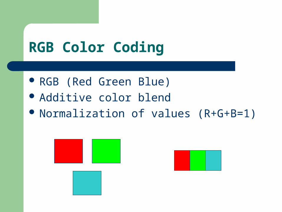
RGB (Red Green Blue) Additive color blend Normalization of values (R+G+B=1)

YUV Color Coding

For the human eye, brightness is more important than color information

Brightnessinformation (Luminance)– 1 channel of luminance (Y)

Color Information (Chrominance)– 2 channels of chrominance (U and V)

Component Coding YUV

Y = 0.30 R + 0.59 G + 0.11 B U = 0.493 (B-Y) V = 0.877 (R-Y) Errors in Y are more severe

– Y to be encoded with high bandwidth

YUV Coding often specified with a raito of the channels (4:2:2)

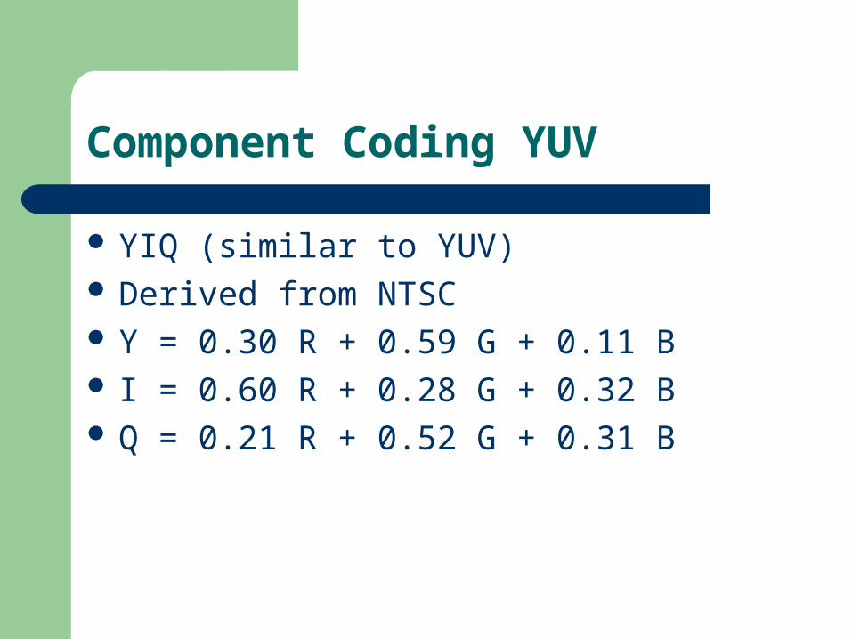
Component Coding YUV

YIQ (similar to YUV) Derived from NTSC Y = 0.30 R + 0.59 G + 0.11 B I = 0.60 R + 0.28 G + 0.32 B Q = 0.21 R + 0.52 G + 0.31 B

Shared Signal

Individual components (RGB, YUV, YIQ) need to be combined to one signal

Methods of modulation to avoid interference

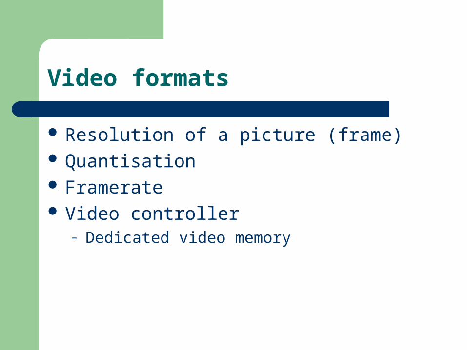
Video formats

Resolution of a picture (frame) Quantisation Framerate Video controller

– Dedicated video memory

Video formats

CGA (Color Graphics Adapter)– 320x200, 4 colors, 16.000 bytes

EGA (Enhanced Graphic Adapter)– 640x350, 16 colors, 112.000 bytes

VGA (Video Graphic Array)– 640x480, 256 colors, 307.200 bytes

XVGA (eXtended Video Graphic Array)– 1024x768, 256 colors, 768.423 bytes

XGA (eXtended Graphic Array)– 1024x768, 16M colors, 2304 kbytes

Many more

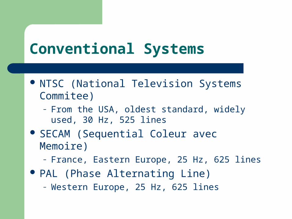
Conventional Systems

NTSC (National Television Systems Commitee)– From the USA, oldest standard, widely used, 30

Hz, 525 lines

SECAM (Sequential Coleur avec Memoire)– France, Eastern Europe, 25 Hz, 625 lines

PAL (Phase Alternating Line)– Western Europe, 25 Hz, 625 lines

High-Definition Television (HDTV)

Resolution– 1440x1152 / 1920x1152

Frame rate– 50 or 60 Hz

No longer interlaced

Digitalisation of video signals

Conversion into a digital representation Nyquist-Theorem (bandwidth = half the

sampling rate)– Of the components

Quantisation 2 Alternatives

– Shared Coding– Component Coding

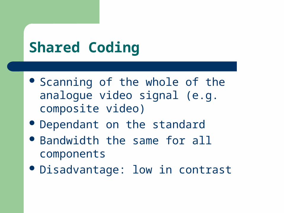
Shared Coding

Scanning of the whole of the analogue video signal (e.g. composite video)

Dependant on the standard Bandwidth the same for all components Disadvantage: low in contrast

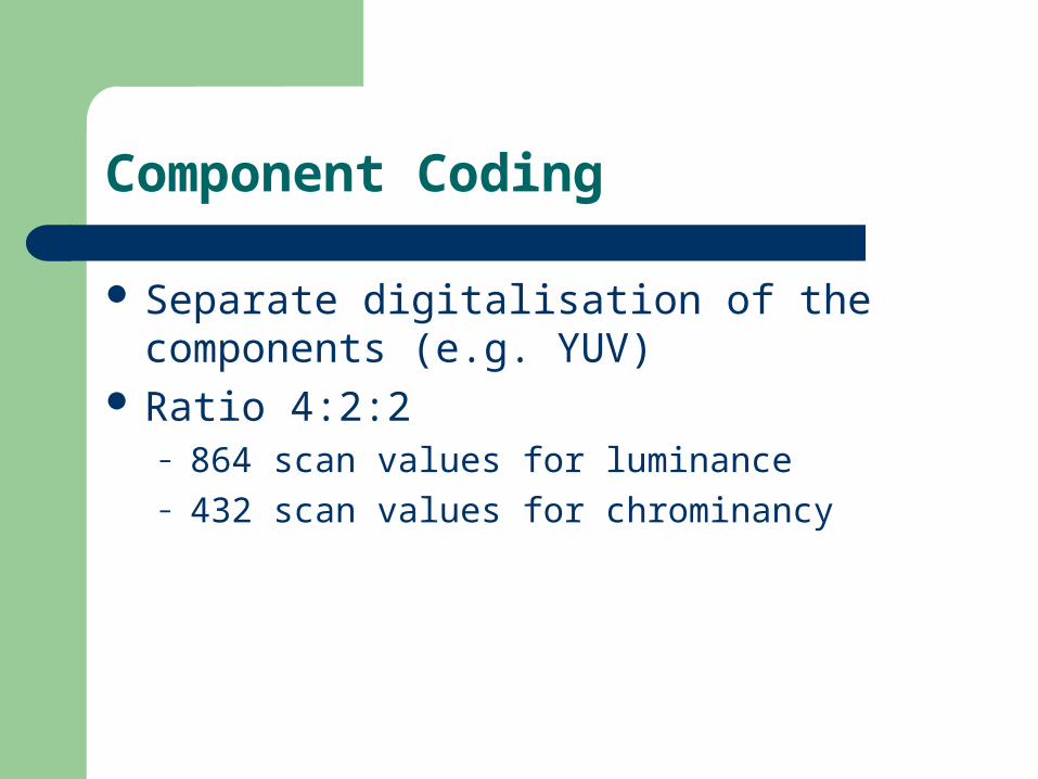
Component Coding

Separate digitalisation of the components (e.g. YUV)

Ratio 4:2:2– 864 scan values for luminance– 432 scan values for chrominancy

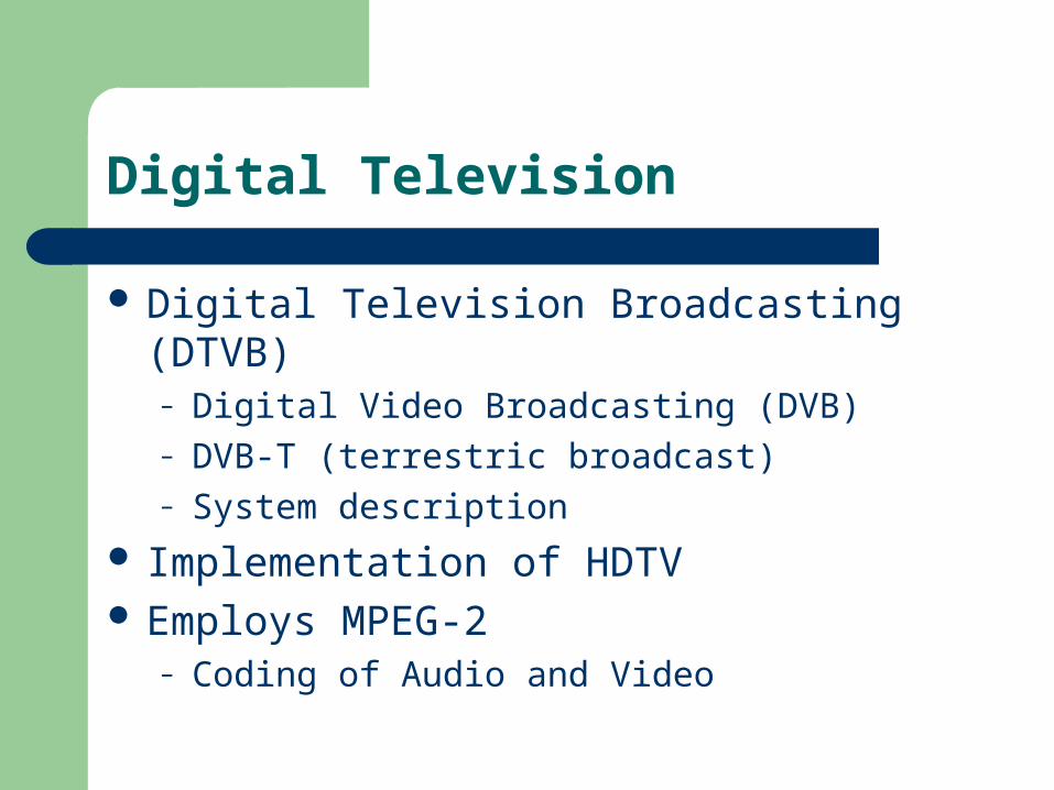
Digital Television

Digital Television Broadcasting (DTVB)– Digital Video Broadcasting (DVB)– DVB-T (terrestric broadcast)– System description

Implementation of HDTV Employs MPEG-2

– Coding of Audio and Video

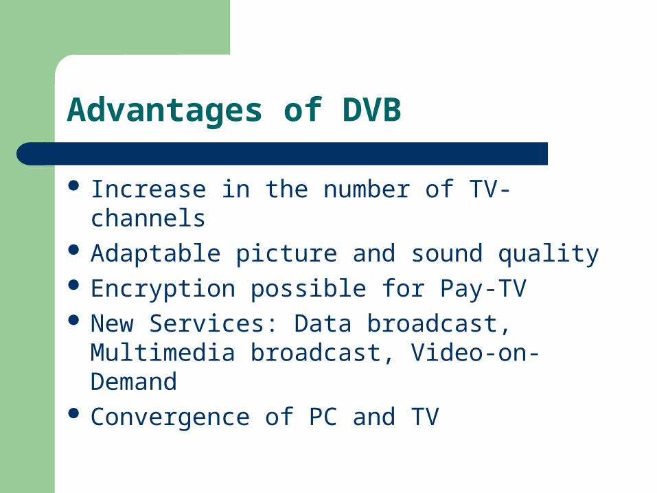
Advantages of DVB

Increase in the number of TV-channels Adaptable picture and sound quality Encryption possible for Pay-TV New Services: Data broadcast, Multimedia

broadcast, Video-on-Demand Convergence of PC and TV

Multimedia: Data Compression

Data Compression

Audio and Video require lots of storage space– Increasing Demand

Text – Single Pictures – Audio – Motion Picture

Data rates influence– Transmission– Processing

Efficient Compression– Theory– Standards

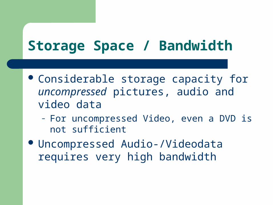
Storage Space / Bandwidth

Considerable storage capacity for uncompressed pictures, audio and video data– For uncompressed Video, even a DVD is not

sufficient

Uncompressed Audio-/Videodata requires very high bandwidth

Required Storage Space

Text– 80 x 60 * 2 bytes = 9600 bytes = 9,4 KByte

Figures– 500 primitives * 5 Bytes for properties = 2500 bytes

Voice– 8 kHz, 8 bit quantisation = 8 kByte / s

Audio– 2 x 44100*16 bit / 8 bit * 1 byte = 172 Kbyte / s

Video– 640 x 480 * 3 x 25 frames = 22,500 Kbyte /s

Important Methods

JPEG (JPEG 2000)– For single pictures

H.261 and H.263– Video sequences of small resolution

MPEG 1,2 and 4– Motion Picture and Audio (MPEG Layer 3)

Demands on Methods

Good quality Small complexity

– Effective implementation

Time boundaries with decompression (and compression)– MPEG-1: high effort with compression

Demands in Dialogue mode

End-to-End latency– Part of the (De-)Compression < 150 ms– 50 ms -> natural dialogue– Additionally all latencies of the network,

communication protocols and of the in- and output devices

Demands in Query mode

Fast Forward / Rewind with simoultaneuos display of the data

Random access to single frames– < 0.5 s– Decompression of single pictures without

interpretation of all the frames before them

Demands in Dialogue and Query mode

Format independent of screen size and refresh rate

Audio and video in different qualities (to adapt to the respective circumstances)

Synchronisation of Audio and Video Implementation in software

Classification of compression methods

Entropy coding– Lossless methods

Source coding– Often lossy

Hybrid coding– Combined application of both of the methods

above for a specific scenario

Entropy coding

Independent of media specific properties Data to compress is a sequence of digital

data values Losslessness

– Data before and after the compression/decompression are identical

Source coding

Usage of the semantics of the information Compression ratio depends on the specific

medium Data before and after the

compressen/decompression are very similar to each other but no longer identical

Hybrid coding

Combination of entroy and souce coding, used e.g. In– JPEG– MPEG– H.263

Decompression

Inverse function of the compression Decompression possible in real time? Symmetric methods

– Similar effort for coding and decoding

Assymetric method– Decoding possible with smaller effort

Run length encoding

Sequence of identical bytes Number of repeating bytes Mark M (e.g. „!“) Stuffing if M is in the data space Example 1: 0, „!“, 256 Example 2: „!“, „!“ (Stuffing) In what cases does it help? Maximum

saving?

Suppression of null values

Special case of run length encoding Selection of a single character that is

repeated often (e.g. „0“) Mark M, after that number of repetitions In what cases does it help? Maximum

saving?

Vector quantisation

Splitting of the data stream into blocks of n bytes

Table with patterns for blocks Index into the table to the entry most similar

to the block Multi-dimensional table -> vector Approximation of the original data stream Example

Pattern Substitution

Patterns of frequent occurence replaced by one byte

Mark M, then index into a table Well suited for text e.g. keywords in programming languages

Diatomic Encoding

Putting together of two bytes of data at a time Determination of the byte-pairs occuring

most frequently e.g. in the English language

– „E“, „T“, „TH“, „RE“, „IN“, ... (8 in total) Special bytes not occuring in the text used to

represent 2 letters Reduction in data of ca. 10%

Static encoding

Frequency of occurence of a character Different coding length for characters Basis of the Morse code Important: unambigous decompression

Huffmann coding

Regards the probability of occurence Minimum number of bits for given probability

of occurence Characters occuring most often get the

shortest code words Binary tree (Nodes contain probabilities,

edges bit 0 or 1)

Huffmann coding

P(A)=0.16, P(B)=0.51, P(C)=0.09, P(D)=0.13 and P(E)=0.11

Huffmann Coding

w(A)=001, w(B)=1, w(C)=011, w(D)=000, w(E)=010

P(ADCEB)=1.0

P(B)=0.51P(ADCE)

P(CE)=0.20 P(AD)=0.29

P(C)=0.09 P(E)=0.11 P(D)=0.13 P(A)=0.16

0 1

10

1 0 0 1

Transformation coding

Data transformed into a better suited mathematical space

Inverse Transformation needs to be possible Discrete Cosine-Transformation (DCT) Fast-Fourier-Transformation (FFT) See example in the JPEG lecture

Prediction or relative encoding

Forming the difference to the previous value Data do not differ much Combination of methods

– e.g. homogenous areas in pictures

DPCM, DM and ADPCM

Further Methods

Color tables– with pictures (video)

Muting– Threshold for sound volume