multiple criteria decision analysis: classification problems … … · · 2006-09-25multiple...
TRANSCRIPT
Multiple Criteria Decision Analysis: Classification
Problems and Solutions
by
Ye Chen
A thesispresented to the University of Waterloo
in fulfilment of thethesis requirement for the degree of
Doctor of Philosophyin
Systems Design Engineering
Waterloo, Ontario, Canada, 2006c© Ye Chen 2006

I hereby declare that I am the sole author of this thesis. This is a true copy ofthe thesis, including any required final revisions, as accepted by my examiners.
I understand that my thesis may be made electronically available to the public.
ii
Abstract
Multiple criteria decision analysis (MCDA) techniques are developed to addresschallenging classification problems arising in engineering management and else-where. MCDA consists of a set of principles and tools to assist a decision maker(DM) to solve a decision problem with a finite set of alternatives compared ac-cording to two or more criteria, which are usually conflicting. The three types ofclassification problems to which original research contributions are made are
(1) Screening: Reduce a large set of alternatives to a smaller set that most likelycontains the best choice.
(2) Sorting: Arrange the alternatives into a few groups in preference order, sothat the DM can manage them more effectively.
(3) Nominal classification: Assign alternatives to nominal groups structured bythe DM, so that the number of groups, and the characteristics of each group,seem appropriate to the DM.
Research on screening is divided into two parts: the design of a sequentialscreening procedure that is then applied to water resource planning in the Region ofWaterloo, Ontario, Canada; and the development of a case-based distance methodfor screening that is then demonstrated using a numerical example.
Sorting problems are studied extensively under three headings. Case-baseddistance sorting is carried out with Model I, which is optimized for use with cardinalcriteria only, and Model II, which is designed for both cardinal and ordinal criteria;both sorting approaches are applied to a case study in Canadian municipal waterusage analysis. Sorting in inventory management is studied using a case-baseddistance method designed for multiple criteria ABC analysis, and then applied to acase study involving hospital inventory management. Finally sorting is applied tobilateral negotiation using a case-based distance model to assist negotiators that isthen demonstrated on a negotiation regarding the supply of bicycle components.
A new kind of decision analysis problem, called multiple criteria nominal classi-fication (MCNC), is addressed. Traditional classification methods in MCDA focuson sorting alternatives into groups ordered by preference. MCNC is the classifi-cation of alternatives into nominal groups, structured by the DM, who specifiesmultiple characteristics for each group. The features, definitions and structures ofMCNC are presented, emphasizing criterion and alternative flexibility. An analysisprocedure is proposed to solve MCNC problems systematically and applied to awater resources planning problem.
iii
Acknowledgments
I would like to give sincere thanks to my thesis supervisors, Drs. Keith W.Hipel and D. Marc Kilgour, for their guidance and financial support. Withouttheir confidence in me, their continuing assistance and encouragement, construc-tive guidance, kind patience, and moral support, I would not have been able toaccomplish this work. It is my great honour to work under their supervision andhave my self-confidence strengthened through this experience.
My thanks also go to my committee members, Drs. David Clausi, DavidFuller and Kumaraswamy Ponnambalam for their constructive comments in thefinal stages of the work. They have been abundantly helpful to me in numerousways. Special thanks are due to my external examiner Dr. Rudolf Vetschera fromUniversity of Vienna for his valuable suggestions that enabled me to improve mythesis.
I cannot end without thanking my parents and my wife for their constant en-couragement and love, on which I have relied throughout the period of this work.
iv

Dedication
This is dedicated to Ms. Xin Su, my beloved wife.
v
Contents
1 Motivation and Objectives 1
1.1 Motivation . . . . . . . . . . . . . . . . . . . . . . . . . . . . . . . . 2
1.2 Objectives . . . . . . . . . . . . . . . . . . . . . . . . . . . . . . . . 4
1.2.1 Screening Problems in MCDA . . . . . . . . . . . . . . . . . 4
1.2.2 Sorting Problems in MCDA . . . . . . . . . . . . . . . . . . 5
1.2.3 Multiple Criteria Nominal Classification . . . . . . . . . . . 6
1.3 Overview of the Thesis . . . . . . . . . . . . . . . . . . . . . . . . . 7
2 Background and Literature Review of Multiple Criteria DecisionAnalysis 10
2.1 Introduction . . . . . . . . . . . . . . . . . . . . . . . . . . . . . . . 10
2.2 MCDA and Relevant Research Topics . . . . . . . . . . . . . . . . . 10
2.3 Analysis Procedures in MCDA . . . . . . . . . . . . . . . . . . . . . 12
2.3.1 The Structure of MCDA Problems . . . . . . . . . . . . . . 12
2.3.2 Decision Maker’s Preference Expressions . . . . . . . . . . . 15
2.4 Summary of MCDA Methods . . . . . . . . . . . . . . . . . . . . . 18
2.4.1 Value Construction Methods . . . . . . . . . . . . . . . . . . 18
2.4.2 Weighting Techniques . . . . . . . . . . . . . . . . . . . . . 19
2.4.3 Aggregation Methods . . . . . . . . . . . . . . . . . . . . . . 20
2.5 Conclusions . . . . . . . . . . . . . . . . . . . . . . . . . . . . . . . 22
vi
3 Screening Problems in Multiple Criteria Decision Analysis 23
3.1 Introduction . . . . . . . . . . . . . . . . . . . . . . . . . . . . . . . 23
3.2 General Description of Screening Problems . . . . . . . . . . . . . . 23
3.3 A Sequential Screening Procedure . . . . . . . . . . . . . . . . . . . 24
3.3.1 Basic Properties . . . . . . . . . . . . . . . . . . . . . . . . . 24
3.3.2 Sequential Screening . . . . . . . . . . . . . . . . . . . . . . 25
3.3.3 Decision Information Based Screening . . . . . . . . . . . . . 26
3.3.4 Pareto Optimality (PO) Based Screening . . . . . . . . . . . 27
3.3.5 Tradeoff Weights (TW) Based Screening . . . . . . . . . . . 28
3.3.6 Non-tradeoff Weights (NTW) Based Screening . . . . . . . . 30
3.3.7 Aspiration Levels (AL) Based Screening . . . . . . . . . . . 32
3.3.8 Data Envelopment Analysis (DEA) Based Screening . . . . . 34
3.3.9 Implementation of Sequential Screening . . . . . . . . . . . . 35
3.4 Case Study: Waterloo Water Supply Planning (WWSP) . . . . . . 36
3.4.1 Screening Procedure . . . . . . . . . . . . . . . . . . . . . . 38
3.4.2 Practical Implementation of WWSP . . . . . . . . . . . . . 40
3.5 Conclusions . . . . . . . . . . . . . . . . . . . . . . . . . . . . . . . 41
4 A Case-based Distance Method for Screening 42
4.1 Introduction . . . . . . . . . . . . . . . . . . . . . . . . . . . . . . . 42
4.2 Case-based Reasoning . . . . . . . . . . . . . . . . . . . . . . . . . 42
4.3 Model Assumptions . . . . . . . . . . . . . . . . . . . . . . . . . . . 43
4.3.1 Case Set Assumptions . . . . . . . . . . . . . . . . . . . . . 43
4.3.2 Distance Assumptions . . . . . . . . . . . . . . . . . . . . . 45
4.4 Model Construction . . . . . . . . . . . . . . . . . . . . . . . . . . . 46
4.5 Distance-based Screening . . . . . . . . . . . . . . . . . . . . . . . . 49
4.5.1 Different Screening Processes . . . . . . . . . . . . . . . . . 49
4.5.2 The Framework of Screening . . . . . . . . . . . . . . . . . . 50
4.6 Numerical Example . . . . . . . . . . . . . . . . . . . . . . . . . . . 52
vii
4.6.1 Background . . . . . . . . . . . . . . . . . . . . . . . . . . . 52
4.6.2 Screening Procedure . . . . . . . . . . . . . . . . . . . . . . 52
4.7 Conclusions . . . . . . . . . . . . . . . . . . . . . . . . . . . . . . . 55
5 Sorting Problems in Multiple Criteria Decision Analysis 57
5.1 Introduction . . . . . . . . . . . . . . . . . . . . . . . . . . . . . . . 57
5.2 General Description of Sorting Problems . . . . . . . . . . . . . . . 57
5.3 Case-based Distance Sorting Model I: Cardinal Criteria . . . . . . . 58
5.3.1 Case Set Assumptions . . . . . . . . . . . . . . . . . . . . . 58
5.3.2 Distance Assumptions . . . . . . . . . . . . . . . . . . . . . 61
5.3.3 Model Construction . . . . . . . . . . . . . . . . . . . . . . . 62
5.3.4 Distance-based Sorting . . . . . . . . . . . . . . . . . . . . . 65
5.3.5 Sorting Consistency . . . . . . . . . . . . . . . . . . . . . . . 66
5.4 Case-based Sorting Model II: Ordinal and Cardinal Criteria . . . . 67
5.4.1 Ordinal Criteria in MCDA . . . . . . . . . . . . . . . . . . . 67
5.4.2 Ordinal Criteria Expressions . . . . . . . . . . . . . . . . . . 68
5.4.3 Case-based Sorting Model Incorporating Ordinal Criteria . . 69
5.4.4 Distance-based Sorting . . . . . . . . . . . . . . . . . . . . . 70
5.4.5 Analysis Procedure for Case-based Distance Sorting . . . . . 70
5.5 Case Study: Canadian Municipal Water Usage Analysis . . . . . . . 71
5.5.1 Background . . . . . . . . . . . . . . . . . . . . . . . . . . . 72
5.5.2 Sorting Procedures . . . . . . . . . . . . . . . . . . . . . . . 75
5.6 Conclusions . . . . . . . . . . . . . . . . . . . . . . . . . . . . . . . 79
6 Sorting Problem Application in Inventory Management 80
6.1 Introduction . . . . . . . . . . . . . . . . . . . . . . . . . . . . . . . 80
6.2 Motivation . . . . . . . . . . . . . . . . . . . . . . . . . . . . . . . . 80
6.3 Multiple Criteria ABC Analysis (MCABC) . . . . . . . . . . . . . . 82
6.4 A Case-based Distance Model for MCABC . . . . . . . . . . . . . . 83
viii
6.4.1 Case Set Definitions for MCABC . . . . . . . . . . . . . . . 83
6.4.2 Distance Assumptions . . . . . . . . . . . . . . . . . . . . . 84
6.4.3 Model Construction . . . . . . . . . . . . . . . . . . . . . . . 86
6.4.4 Distance-based Sorting . . . . . . . . . . . . . . . . . . . . . 90
6.4.5 Post-optimality Analyses . . . . . . . . . . . . . . . . . . . . 91
6.5 A Case Study in Hospital Inventory Management . . . . . . . . . . 93
6.5.1 Background . . . . . . . . . . . . . . . . . . . . . . . . . . . 93
6.5.2 Selection of Case Sets . . . . . . . . . . . . . . . . . . . . . . 94
6.5.3 Model Construction . . . . . . . . . . . . . . . . . . . . . . . 94
6.5.4 Post-optimality Analyses . . . . . . . . . . . . . . . . . . . . 100
6.5.5 Comparisons and Explanation . . . . . . . . . . . . . . . . . 105
6.6 Conclusions . . . . . . . . . . . . . . . . . . . . . . . . . . . . . . . 106
7 Sorting Problem Extension in Negotiation 107
7.1 Introduction . . . . . . . . . . . . . . . . . . . . . . . . . . . . . . . 107
7.2 Motivation . . . . . . . . . . . . . . . . . . . . . . . . . . . . . . . . 107
7.3 Multiple Issue Bilateral Negotiations . . . . . . . . . . . . . . . . . 109
7.4 A Case-based Distance Model for Bilateral Negotiation . . . . . . . 110
7.4.1 Case Set Assumptions . . . . . . . . . . . . . . . . . . . . . 110
7.4.2 Distance Assumptions . . . . . . . . . . . . . . . . . . . . . 110
7.4.3 Distance Intervals for Linguistic Grades . . . . . . . . . . . . 111
7.4.4 Weight Determination and Distance Construction . . . . . . 112
7.4.5 Post-optimality Analyses . . . . . . . . . . . . . . . . . . . . 115
7.4.6 Distance-based Bilateral Negotiation Support System . . . . 116
7.4.7 Generating the Suggested Alternative Set . . . . . . . . . . . 118
7.4.8 Representing Preferences and Negotiating Using Distances . 118
7.4.9 Checking the Efficiency of the Compromise . . . . . . . . . . 121
7.5 Case Study: A Bicycle Component Negotiations . . . . . . . . . . . 121
7.5.1 Background . . . . . . . . . . . . . . . . . . . . . . . . . . . 121
ix
7.5.2 Initial Parameter Settings . . . . . . . . . . . . . . . . . . . 122
7.5.3 Case Set Acquisition and Computations for DM1 . . . . . . 123
7.5.4 Post-optimality Analyses for DM1 . . . . . . . . . . . . . . . 124
7.5.5 Case Set Acquisition and Computations for DM2 . . . . . . 125
7.5.6 Generating Suggested Alternative Set . . . . . . . . . . . . . 127
7.5.7 Checking the Efficiency of the Compromise Alternative . . . 127
7.6 Conclusions . . . . . . . . . . . . . . . . . . . . . . . . . . . . . . . 128
8 Multiple Criteria Nominal Classification 129
8.1 Introduction . . . . . . . . . . . . . . . . . . . . . . . . . . . . . . . 129
8.2 Motivation . . . . . . . . . . . . . . . . . . . . . . . . . . . . . . . . 129
8.3 Features, Definition, Structures, and Properties of MCNC . . . . . . 130
8.3.1 Illustrative Examples of MCNC . . . . . . . . . . . . . . . . 130
8.3.2 Features of MCNC . . . . . . . . . . . . . . . . . . . . . . . 131
8.3.3 Preliminary Definitions . . . . . . . . . . . . . . . . . . . . . 132
8.3.4 Definition and Structures of MCNC . . . . . . . . . . . . . . 132
8.3.5 Properties of MCNC . . . . . . . . . . . . . . . . . . . . . . 135
8.3.6 Types of Classification . . . . . . . . . . . . . . . . . . . . . 139
8.4 MCNC Analysis Procedure . . . . . . . . . . . . . . . . . . . . . . . 140
8.4.1 Analysis Procedure for MCNC . . . . . . . . . . . . . . . . . 140
8.5 A Linear Additive Value Function Approach to MCNC . . . . . . . 142
8.5.1 Model Assumptions . . . . . . . . . . . . . . . . . . . . . . . 142
8.5.2 Objective Function . . . . . . . . . . . . . . . . . . . . . . . 143
8.5.3 Constraints . . . . . . . . . . . . . . . . . . . . . . . . . . . 143
8.6 Numerical Example: Water Supply Planning . . . . . . . . . . . . . 145
8.6.1 Problem Descriptions . . . . . . . . . . . . . . . . . . . . . . 145
8.6.2 Post-criteria Assessment . . . . . . . . . . . . . . . . . . . . 146
8.6.3 Alternative Identification . . . . . . . . . . . . . . . . . . . . 147
8.6.4 Decision Maker’s Preferences . . . . . . . . . . . . . . . . . . 148
x
8.6.5 Value Function . . . . . . . . . . . . . . . . . . . . . . . . . 150
8.6.6 Classification Analysis . . . . . . . . . . . . . . . . . . . . . 150
8.7 Conclusions . . . . . . . . . . . . . . . . . . . . . . . . . . . . . . . 152
9 Contributions and Future Research 153
9.1 Main Contributions of the Thesis . . . . . . . . . . . . . . . . . . . 153
9.2 Suggestions for Future Research . . . . . . . . . . . . . . . . . . . . 155
Bibliography 157
xi
List of Figures
1.1 Problematiques in MCDA, adapted from Doumpos and Zopouidis(2002) . . . . . . . . . . . . . . . . . . . . . . . . . . . . . . . . . . 4
1.2 Contents of This Thesis . . . . . . . . . . . . . . . . . . . . . . . . 8
2.1 The Structure of an MCDA Problem . . . . . . . . . . . . . . . . . 13
2.2 Different Approaches to Obtaining Values . . . . . . . . . . . . . . 18
2.3 Methods of Weight Construction . . . . . . . . . . . . . . . . . . . 20
2.4 Preference Acquisition and Aggregation in MCDA . . . . . . . . . . 21
3.1 The Relationship among Screening, Sorting and Choice . . . . . . . 24
3.2 Screening Methods and Decision Information . . . . . . . . . . . . . 26
3.3 Frontier Analyst Based DEA Screening . . . . . . . . . . . . . . . . 39
3.4 Screening Methods and Information Available . . . . . . . . . . . . 41
4.1 The Idea of Case-based Screening . . . . . . . . . . . . . . . . . . . 44
4.2 Distances and the Case Set . . . . . . . . . . . . . . . . . . . . . . . 47
4.3 Analysis Procedure for Case-based Distance Screening . . . . . . . . 51
5.1 Relationships Among A and S . . . . . . . . . . . . . . . . . . . . . 59
5.2 The Idea of Case-based Sorting . . . . . . . . . . . . . . . . . . . . 60
5.3 The Distances R and D(Ai)+ . . . . . . . . . . . . . . . . . . . . . 63
5.4 Analysis Procedure for Case-based Distance Sorting . . . . . . . . . 71
5.5 z+ Method Results . . . . . . . . . . . . . . . . . . . . . . . . . . . 78
xii
5.6 z− Method Results . . . . . . . . . . . . . . . . . . . . . . . . . . . 78
6.1 Example of Dollar Usage Distribution Curve . . . . . . . . . . . . . 82
6.2 The Joint Matrix for Two Criteria . . . . . . . . . . . . . . . . . . . 83
6.3 The Idea of Case-based Distance model . . . . . . . . . . . . . . . . 85
6.4 Relationships Among R+A, R+
B and D(Ai)+ . . . . . . . . . . . . . . 87
6.5 The Joint Matrix for Two MCABC Methods . . . . . . . . . . . . . 91
7.1 Relationships Among Zrk , A+
k and A−k . . . . . . . . . . . . . . . . . . 113
7.2 The Procedure of Negotiation Support System. . . . . . . . . . . . 117
7.3 Obtaining Alternatives When 8 ≤ |A1 ∩ A2| ≤ 10. . . . . . . . . . . 119
7.4 Obtaining Alternatives When |A1 ∩ A2| < 8. . . . . . . . . . . . . . 119
7.5 Obtaining Alternatives When |A1 ∩ A2| > 10. . . . . . . . . . . . . 120
7.6 Negotiating Using Distances. . . . . . . . . . . . . . . . . . . . . . . 120
7.7 A∗ is An Efficient Alternative. . . . . . . . . . . . . . . . . . . . . . 121
7.8 A∗ is An Inefficient Alternative. . . . . . . . . . . . . . . . . . . . . 122
7.9 The Proportions of Different Alternatives for DM1. . . . . . . . . . 125
7.10 The Proportions of Different Alternatives for DM2. . . . . . . . . . 127
8.1 Criteria Sets for the Two Groups . . . . . . . . . . . . . . . . . . . 131
8.2 The Classification of Ten Applicants . . . . . . . . . . . . . . . . . 131
8.3 The Structures of MCNC . . . . . . . . . . . . . . . . . . . . . . . . 133
8.4 Analysis Procedure for MCNC Problems . . . . . . . . . . . . . . . 141
8.5 The Criteria Set of WWSP . . . . . . . . . . . . . . . . . . . . . . . 146
xiii
List of Tables
2.1 MCDA and Relevant Research Topics . . . . . . . . . . . . . . . . . 11
3.1 Information Requirements for Different Screening Methods . . . . . 35
3.2 The Basic Structure of the WWSP . . . . . . . . . . . . . . . . . . 37
3.3 Value Data of Reduced WWSP . . . . . . . . . . . . . . . . . . . . 38
3.4 Tradeoff Weights Based Screening . . . . . . . . . . . . . . . . . . . 40
4.1 The Basic Information of Alternatives . . . . . . . . . . . . . . . . . 53
4.2 The case set for screening . . . . . . . . . . . . . . . . . . . . . . . 53
4.3 The Distances on Each Criterion in the Case Set . . . . . . . . . . . 54
4.4 Distances of Alternatives to the Centroid on Each Criterion . . . . 55
4.5 Distances of Alternatives from the Centroid . . . . . . . . . . . . . 55
4.6 Threshold Screening for Each Alternative . . . . . . . . . . . . . . . 56
5.1 Linguistic Evaluation Grade and Value Interval for z+ Sorting Method 68
5.2 Case Set for MWUA . . . . . . . . . . . . . . . . . . . . . . . . . . 74
5.3 Consequences of Cardinal Criteria in the Case Set . . . . . . . . . . 74
5.4 Linguistic Evaluations in the Case Set . . . . . . . . . . . . . . . . 75
5.5 Centroid of the Case Set . . . . . . . . . . . . . . . . . . . . . . . . 75
5.6 The Distances on Each Criterion . . . . . . . . . . . . . . . . . . . 76
6.1 Listing of SKUs with Multiple Criteria, adapted from Flore et al.(1992) . . . . . . . . . . . . . . . . . . . . . . . . . . . . . . . . . . 95
xiv
6.2 The Basic Information Settings . . . . . . . . . . . . . . . . . . . . 96
6.3 The Normalized Consequence Data of Case Sets for A+MCABC . . 96
6.4 The Normalized Consequence Data of Case Sets for A−MCABC . . 97
6.5 The Results of A+ABC and A−ABC Classification . . . . . . . . . . 99
6.6 Post-optimality Analyses and Final Solutions for A+MCABC . . . . 100
6.7 Percentage Value Method Based Post-optimality Analyses for A+ABC101
6.8 Post-optimality Analyses and Final Solutions for A−MCABC . . . . 102
6.9 Percentage Value Method Based Post-optimality Analyses for A−ABC103
6.10 The Final Sorting Results for the Percentage Value Method . . . . 104
6.11 Comparison of Results with the Flores et al. Method (Flore et al.,1992) . . . . . . . . . . . . . . . . . . . . . . . . . . . . . . . . . . 105
7.1 Negotiation Initial Settings . . . . . . . . . . . . . . . . . . . . . . . 122
7.2 The Case Set Provided by DM1 . . . . . . . . . . . . . . . . . . . . 123
7.3 Normalized Distances for DM1 . . . . . . . . . . . . . . . . . . . . 123
7.4 Post-optimality Analyses and Final Solutions DM1 . . . . . . . . . 125
7.5 The Case Set Provided by DM2 . . . . . . . . . . . . . . . . . . . . 125
7.6 Normalized Distances for DM2 . . . . . . . . . . . . . . . . . . . . 126
7.7 Initial Suggested Alternative Set T . . . . . . . . . . . . . . . . . . 127
7.8 Updated Suggested Alternative Set T . . . . . . . . . . . . . . . . . 128
8.1 MCNC Problems Classification . . . . . . . . . . . . . . . . . . . . 139
8.2 The Basic Structure of the WWSP . . . . . . . . . . . . . . . . . . 148
8.3 The Values of Alternatives for Near-future project . . . . . . . . . . 148
8.4 The Values of Alternatives for Mid-term and Long-term project . . 149
xv
Chapter 1
Motivation and Objectives
The study of decision making is part of many of disciplines, including psychology,business, engineering, operations research, systems engineering, and managementscience. As society becomes more complex, the need for decisions that balanceconflicting objectives (criteria) has grown. Government policy decisions, for exam-ple, which regulate growth, employment, and general welfare, have always facedthis problem. Businesses encountering strategic decisions must consider multipleobjectives as well; although short-run profit is important, long-run factors such asmarket position, product quality, and development of production capability oftenconflict with it.
Decision has attracted the attention of many thinkers since ancient times. Thegreat philosophers Aristotle, Plato, and Thomas Aquinas, discussed the capacityof humans to decide and claimed that contemplation is what distinguishes humansfrom animals (Figueira et al., 2005). To illustrate some important aspects of deci-sion, consider a quote a letter from Benjamin Franklin to Joseph Priestley whichhas been taken from a paper by MacCrimmon (1973).
London, Sept 19, 1772Dear Sir,In the affair of so much importance to you, wherein you ask my advice, I cannot,for what of sufficient premise, advise you want to determine, but if you please Iwill tell you how. [· · · ] When I have thus columns; writing over the one Pro, andover the other Con. [· · · ] When I have thus got them all together in one view, Iendeavor to estimate their respective weights; and where I find two, one on eachside, that seem equal, I strike them both out. If I find a reason pro equal to sometwo reasons con, I strike out the three. If I judge some two reasons con, equal tothree reasons pro, I strike out the five; and thus proceeding I find at length where
1
the balance lies; and if, after a day or two of further consideration, nothing newthat is of importance occurs on either side, I come to a determination accordingly.[· · · ] I have found great advantage from this kind of equation, and what might becalled moral or prudential algebra. Wishing sincerely that you may determine forthe best, I am ever, my dear friend, yours most affectionately.B. Franklin
What is of interest in the above quotation is the fact that decision is stronglyrelated to the comparison of different points of view, for which some are in favorand some are against. During the last forty years, systematic methodologies tolook at such decision problems have caught the attention of many researchers. Theapproach recommended by Franklin, which explicitly takes into account the prosand the cons of different points of view, is the domain of multiple criteria decisionanalysis (MCDA).
Similar terms for describing this type of decision assistance include “multiplecriteria decision aid” which comes from Europe (Roy, 1985; Vincke, 1992) and “mul-tiple objective decision making” which is more widely used in the North America.The field of MCDA refers to the wide variety of tools and methodologies devel-oped for the purpose of helping a decision maker (DM) to select from finite sets ofalternatives according to two or more criteria, which are usually conflicting.
1.1 Motivation
The first and the most important step for studying a multiple criteria decisionproblem is the identification of a problematique, which was first introduced intoMCDA by Roy (1985). The French word, “problematique” means fundamentalproblems and been translated as problematics in English by some researchers.The following was written by Roy (1996) as an explanation of problematics inMCDA.
The analyst must now determine in what terms he will pose the problem. Whattypes of results does he envision and how does he see himself fitting into the de-cision process to aid in arriving at these results? Towards what will he direct hisinvestigation? What form does he foresee his recommendation taking? ...We usethe word problematic to describe the analyst’s conception of the way he envisionsthe aid he will supply in the problem at hand based on answers to these questions.
Furthermore, Roy (1985, p.57) proposed four different kinds of problems asproblematiques in MCDA — P. α, P. β, P. γ, P. δ.
2
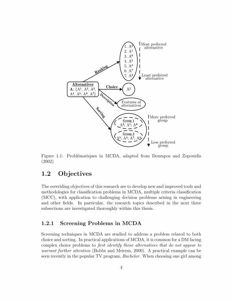
Definition 1. • P. α, choice. Choosing one alternative from a set of alternative,A.
• P. β, sorting. Sorting alternatives in predefined homogenous groups whichare given in a preference order.
• P. γ, ranking. Ranking alternatives from best to worst.
• P. δ, description. Describing alternatives in terms of their major distin-guishing features.
Figure 1.1 provides an intuitive example of problematiques in MCDA. In theexample, there are seven alternatives available for a particular multiple criteriadecision analysis. In ranking analysis, the whole ordering sequence of alternativesA1 to A7, from most to least preferred, is listed as A2 ≻ A1 ≻ A6 ≻ A5 ≻ A4 ≻A7 ≻ A3, where ≻ means preferred to. For choice analysis, the best alternativeis chosen as A2. Under the category of description, one can describe features ofalternatives. Within sorting analysis, one classifies all alternatives into two groupsin which Group 1 (A1, A2, A6) is preferred to Group 2 (A3, A4, A5, A7).
Three problematiques consisting of choice, sorting and ranking can lead to spe-cific results implying regarding evaluations of alternatives. Some of these problematiqueshave been widely studied during the last thirty years. For example, methods forsolving choice and ranking problems are so common that many researchers (forexample, Olson (1996) in the book Decision Aids for Selection Problems) assumethat they are the only problems of MCDA and do not distinguish problematiquesexplicitly, while substantial research on the sorting problem has not been carriedout until recently.
Some new methods (Doumpos and Zopounidis, 1998; Slowinski and Zopounidis,1995; Zopounidis and Doumpos, 2002) or revisions of well-known methods (Belacel,2000; Yu, 1992) have recently been put forward to solve sorting problems. However,a systematic analysis of classification problems including sorting has not been wellstudied. For example, relationships among choice, sorting and ranking problemshave never been investigated. In this thesis, a general research scheme involvingclassification problems in MCDA is systematically addressed and some practicalapplications are studied to demonstrate the proposed methodologies. The key ob-jectives are outlined in the next section.
3
Most preferred alternative
Least preferred alternative
Alternatives
A: {A1, A2, A3,A4, A5, A6, A7}
1. A2
2. A1
3. A6
4. A5
5. A4
6. A7
7. A3
A2
Features of alternatives
Group 1
A2; A1; A6
Group 2
A5; A4; A7; A3
More preferred group
Less preferred group
Rankin
g
Choice
Description
Sorting
Figure 1.1: Problematiques in MCDA, adapted from Doumpos and Zopouidis(2002)
1.2 Objectives
The overriding objectives of this research are to develop new and improved tools andmethodologies for classification problems in MCDA, multiple criteria classification(MCC), with application to challenging decision problems arising in engineeringand other fields. In particular, the research topics described in the next threesubsections are investigated thoroughly within this thesis.
1.2.1 Screening Problems in MCDA
Screening techniques in MCDA are studied to address a problem related to bothchoice and sorting. In practical applications of MCDA, it is common for a DM facingcomplex choice problems to first identify those alternatives that do not appear towarrant further attention (Bobbs and Meierm, 2000). A practical example can beseen recently in the popular TV program, Bachelor. When choosing one girl among
4
several, a young man solves it by sequential elimination (screening) of one girl fromfurther consideration. The choice is expressed by not assigning this girl a rose,while the others each get one.
Screening techniques can be regarded as useful MCDA methods, leading toa final choice. They apply when not enough information is available to reach afinal choice directly, or too many alternatives must be considered. The number ofalternatives to be taken into account further is dramatically reduced if screening iscarried out properly reducing the work load for the DM. Screening techniques aredesigned to solve some sorting problems, and can help the DM simplify the finalchoice problem.
During the past few decades several different methods have been separatelyput forward to deal with screening problems. But there has been no systematicexploration of this topic in the literature, and researchers on sorting have paidlittle attention to it.
In summary, in this research topic the screening problem will be investigatedsystemically. Feasible screening methods are summarized according to the infor-mation provided by the DM, and are integrated into a unified framework, thesequential screening procedure (Chen et al., 2005b). The efficacy of this structureis demonstrated using a water resources planning problem. Also, a new and usefulmethod, the case-based distance model, is proposed to solve screening problemsand illustrated with a numerical example (Chen et al., 2005c).
1.2.2 Sorting Problems in MCDA
Practical applications of sorting include financial management such as businesscredit risk assessment; marketing analysis, such as customer satisfaction measure-ment; environmental and energy management, such as the analysis, measurementand classification of environmental impacts of different policies (Zopounidis andDoumpos, 2002). This rich range of potential real world applications has encour-aged researchers to develop innovative methodologies for sorting. With the evolu-tion of MCDA and the appearance of powerful new tools to deal with classifica-tion, research on sorting in MCDA is now receiving more attention. For exampleDoumpos and Zopouidis (2002) wrote the first book on sorting in MCDA. Kilgouret al. (2003) studied the problem of screening (two-group sorting) alternatives insubset selection problems. Zopounidis and Doumpos (2002) gave a comprehensiveliterature review of sorting in MCDA.
Generally speaking, there are two kinds of sorting methods: direct judgment
5
methods and case-based reasoning methods. In direct judgement methods, a par-ticular decision model is employed and the DM directly provides enough informationto evaluate all preferential parameters in the model. In case-based reasoning meth-ods, the DM furnishes decisions for selected cases, which determine preferentialparameters to calibrate a chosen procedure as consistently as possible.
Direct judgement methods include ELECTRE TRI (Yu, 1992) and N-TOMIC(Massaglia and Ostanello, 1991). Both belong to the family of ELECTRE methodsinitially introduced by Roy (1968), but feature some theoretical modifications to ad-dress sorting. Case-based reasoning methods include UTADIS, MHDIS (Doumposand Zopouidis, 2002) and the rough set method (Slowinski, 2001). UTADIS andMHDIS use the UTA (UTilites Additives) (Jacquet-Lagreze and Siskos, 1982) tech-nique to sort alternatives; the rough set method employs rough set theory, as de-veloped by Slowinski (2001), for sorting.
In summary, within this research topic new techniques, case-based distancemethods for sorting, are developed to solve problems (Chen et al., 2005d, 2004).The advantages of this method include (1) clear geometric meaning, so the DM caneasily understand the method; (2) expeditious and accurate elicitation of the DM’spreferences, which is much more efficient than direct inquiry. Then the applica-tions of this method in inventory management (Chen et al., 2005e), and bilateralnegotiation (Chen et al., 2005f) are investigated.
1.2.3 Multiple Criteria Nominal Classification
Current research on classification problems in MCDA mainly focuses on sorting,in which alternatives are assigned to groups defined ordinally by the DM. Anotherpractical decision problem is to assign alternatives to homogeneous groups definednominally. For example, in human resources management, some job applicantsshould be assigned to appropriate occupation groups according to their multiplequalifications (criteria). This kind of problem is called Multiple Criteria NominalClassification (MCNC) to distinguish it from the sorting problem in MCDA.
To date, only a few papers are relevant to MCNC, such as those of Perny (1998),Scarelli and Narula (2000), and Malakooti and Yang (2004). One reason may bethat distinctions between MCNC and other classification areas have not been clar-ified. Note that similar multiple criteria (multidimensional) classification problems(which can be termed multiple attribute classification, MAC) have been widelystudied in other research areas such as statistical learning and pattern recogni-tion, medical diagnosis, handwriting and voice recognition (Zervakis et al., 2004).
6
But there are great differences between sorting and MAC. As a decision analysismethod, sorting is a prescriptive approach to assist individuals to make wise classi-fication decisions, while MAC is a descriptive approach to detect and characterizegeneral similarities within a large set of data. Sorting involves determining theDM’s preferences in decision situations; MAC does not have this function.
Overall, this research area focuses on the theoretical extension of sorting prob-lems (Chen et al., 2006), as follows: (1) the systematic modelling of the MCNCproblems is presented including their features, definition and structures; and (2)the development of techniques to solve MCNC problems is addressed and a wa-ter resources planning problem is studied to demonstrate the proposed analysisprocedure.
1.3 Overview of the Thesis
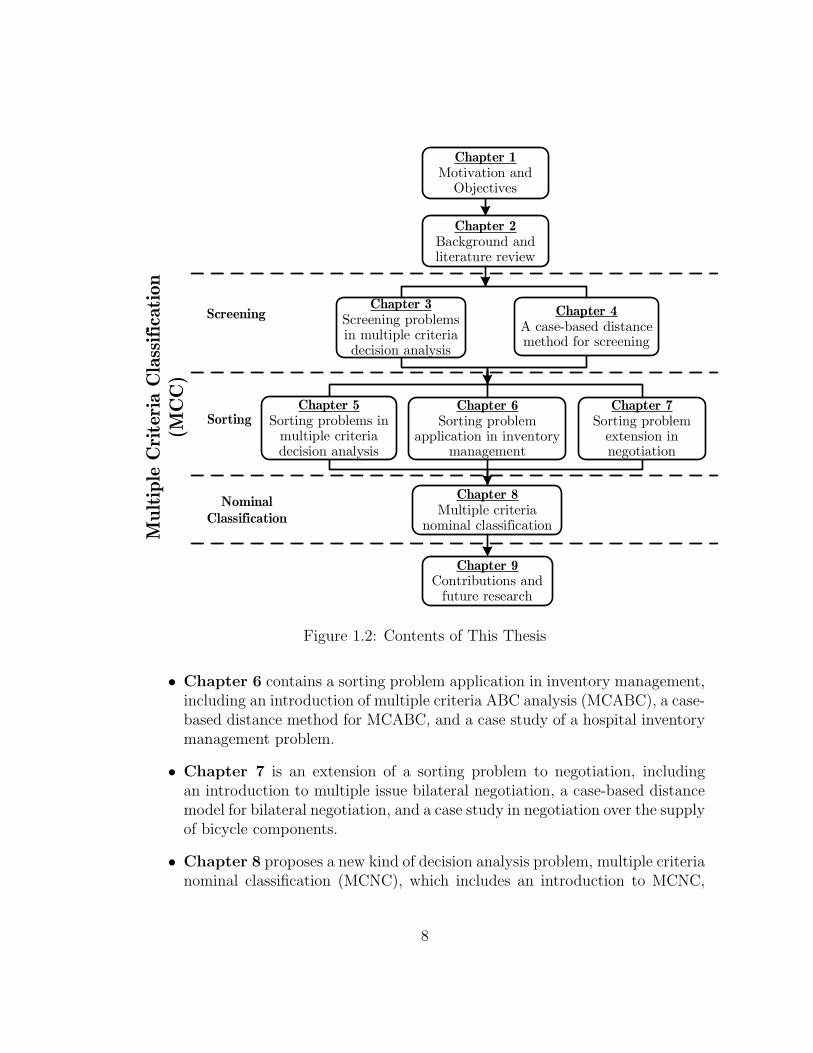
Figure 1.2 summarizes of the organization of the thesis. A detailed explanationfollows:
• Chapter 1 describes the motivation and objectives of this thesis, includinga discussion of problematiques in MCDA and the organization of the thesis.
• Chapter 2 is a background and literature review of MCDA, including thefollowing: MCDA and relevant research topics, analysis procedures in MCDA,and a summary of MCDA methods.
• Chapter 3 addresses screening problems in MCDA, including general de-scriptions of screening problem, a systematic sequential screening procedure,and a case study of water resource planning in the Regional Municipality ofWaterloo.
• Chapter 4 introduces a case-based distance model for screening and a nu-merical example to demonstrate the proposed procedure.
• Chapter 5 focuses on sorting problems in MCDA, including general descrip-tions of the sorting problem, case-based distance model I for cardinal criteria,case-base distance model II for both cardinal and ordinal criteria, and a casestudy analyzing Canadian municipal water usage.
7
Chapter 1Motivation and
Objectives
Chapter 2Background and literature review
Chapter 3Screening problems in multiple criteria decision analysis
Chapter 4A case-based distance method for screening
Chapter 5Sorting problems in
multiple criteria decision analysis
Chapter 6Sorting problem
application in inventory management
Chapter 7Sorting problem
extension in negotiation
Chapter 8Multiple criteria
nominal classification
Chapter 9Contributions and
future research
Screening
Sorting
Nominal Classification
Multip
le C
rite
ria C
lass
ific
atio
n(M
CC
)
Figure 1.2: Contents of This Thesis
• Chapter 6 contains a sorting problem application in inventory management,including an introduction of multiple criteria ABC analysis (MCABC), a case-based distance method for MCABC, and a case study of a hospital inventorymanagement problem.
• Chapter 7 is an extension of a sorting problem to negotiation, includingan introduction to multiple issue bilateral negotiation, a case-based distancemodel for bilateral negotiation, and a case study in negotiation over the supplyof bicycle components.
• Chapter 8 proposes a new kind of decision analysis problem, multiple criterianominal classification (MCNC), which includes an introduction to MCNC,
8

an MCNC analysis procedure, a linear additive value function approach toMCNC, and a numerical example to demonstrate the procedure.
• Chapter 9 contains a summary of the main contributions of the researchand suggestions for future research.
9
Chapter 2
Background and LiteratureReview of Multiple CriteriaDecision Analysis
2.1 Introduction
In this chapter, a background and literature review of MCDA are presented toprovide a foundation for the research in this thesis. MCDA and relevant researchtopics are first explained briefly, and then an analysis procedure is proposed thatprovides a systematic framework for MCDA. This permits many approaches toMCDA to be summarized and integrated into one system. This chapter is basedupon the research of Chen et al. (2004).
2.2 MCDA and Relevant Research Topics
Every decision situation exists within a context. This environment consists of aset of circumstances and conditions that affect the manner in which the decisionmaking problem can be resolved. Radford (1989) and Hipel et al. (1993) suggestedfour major factors that determine the context, namely:
1. Whether or not uncertainty is present,
2. Whether or not the benefits and costs resulting from the implementation ofpotential courses of actions can be entirely assessed in quantitative terms,
10
3. Whether one criterion or multiple criteria must be taken into account,
4. Whether the power to make the decision is under the control of one organi-zation, individual or group, or whether two or more of the participants havepower to influence the decision.
Based on these factors, Radford (1989) and Hipel et al. (1993) focused on threedecision analysis scenarios: single participant-multiple criteria, multiple participant-single criterion, and multiple participant-multiple criteria situations. Here, thisclassification is extended and a systematic discussion of the relationship of MCDAand its related research topics is presented.
Table 2.1: MCDA and Relevant Research Topics
Single Criterion Multiple Criteria
Single DM SDSC SDMC
Multiple DMs MDSC MDMC
Infinitely Many DMs IDSC IDMC
Finite Alternatives FASC FAMC
Infinitely Many Alternatives IASC IAMC
Table 2.1 presents the acronyms used for the various decision situations thatarise in practice. The characteristics or commonalities of these decision situationsare discussed below.
• SDSC and FASC: a single DM a single criterion, and finite alternativesproblem. SDSC and FASC are simple decision problems, in which a DMsolely considers one criterion to make decisions. SDSC related research top-ics include cost-benefit analysis in engineering economics and traditional oneobjective optimization based decision in operation research.
• SDMC and FAMC: a single DM with multiple criteria, and finite alterna-tives problem. Here one categorizes SDMC and FAMC as the MCDA studiedin this thesis. The areas of SDMC and FAMC overlap with much of theMCDA research presented in this thesis.
• MDSC and MDMC: a multiple DM with single criterion or multiple criteriaproblem. MDSC and MDMC have a finite number of DMs who are involved in
11
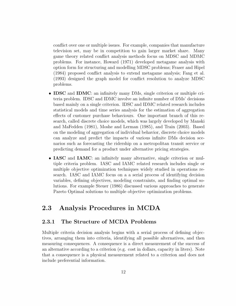
conflict over one or multiple issues. For example, companies that manufacturetelevision set, may be in competition to gain larger market share. Manygame theory related conflict analysis methods focus on MDSC and MDMCproblems. For instance, Howard (1971) developed metagame analysis withoption form for structuring and modelling MDSC problems; Fraser and Hipel(1984) proposed conflict analysis to extend metagame analysis; Fang et al.(1993) designed the graph model for conflict resolution to analyze MDSCproblems.
• IDSC and IDMC: an infinitely many DMs, single criterion or multiple cri-teria problem. IDSC and IDMC involve an infinite number of DMs’ decisionsbased mainly on a single criterion. IDSC and IDMC related research includesstatistical models and time series analysis for the estimation of aggregationeffects of customer purchase behaviours. One important branch of this re-search, called discrete choice models, which was largely developed by Manskiand MaFedden (1981), Moshe and Lerman (1985), and Train (2003). Basedon the modeling of aggregation of individual behavior, discrete choice modelscan analyze and predict the impacts of various infinite DMs decision sce-narios such as forecasting the ridership on a metropolitan transit service orpredicting demand for a product under alternative pricing strategies.
• IASC and IAMC: an infinitely many alternative, single criterion or mul-tiple criteria problem. IASC and IAMC related research includes single ormultiple objective optimization techniques widely studied in operations re-search. IASC and IAMC focus on a a serial process of identifying decisionvariables, defining objectives, modeling constraints, and finding optimal so-lutions. For example Steuer (1986) discussed various approaches to generatePareto Optimal solutions to multiple objective optimization problems.
2.3 Analysis Procedures in MCDA
2.3.1 The Structure of MCDA Problems
Multiple criteria decision analysis begins with a serial process of defining objec-tives, arranging them into criteria, identifying all possible alternatives, and thenmeasuring consequences. A consequence is a direct measurement of the success ofan alternative according to a criterion (e.g. cost in dollars, capacity in liters). Notethat a consequence is a physical measurement related to a criterion and does notinclude preferential information.
12
The process of structuring MCDA problems has received a great deal of atten-tion. von Winterfeldt (1980) called problem structuring the most difficult part ofdecision aid. Keeney (1992) and Hammond et al. (1999) proposed a systematicanalysis method, value-focused thinking, which provided an excellent approachto this aspect of MCDA.
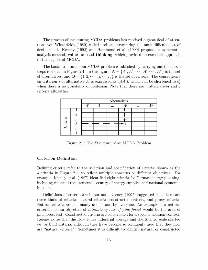
The basic structure of an MCDA problem established by carrying out the abovesteps is shown in Figure 2.1. In this figure, A = {A1, A2, · · · , Ai, · · · , An} is the setof alternatives, and Q = {1, 2, · · · , j, · · · , q} is the set of criteria. The consequenceon criterion j of alternative Ai is expressed as cj(A
i), which can be shortened to cij
when there is no possibility of confusion. Note that there are n alternatives and qcriteria altogether.
A1 A2 ... Ai ... An
2
...
...Cri
teri
a
Alternatives
1
j
q
icj
Figure 2.1: The Structure of an MCDA Problem
Criterion Definition
Defining criteria refer to the selection and specification of criteria, shown as theq criteria in Figure 2.1, to reflect multiple concerns or different objectives. Forexample, Keeney et al. (1987) identified eight criteria for German energy planning,including financial requirements, security of energy supplies and national economicimpacts.
Definitions of criteria are important. Keeney (1992) suggested that there arethree kinds of criteria, natural criteria, constructed criteria, and proxy criteria.Natural criteria are commonly understood by everyone. An example of a naturalcriterion for an objective of minimizing loss of pine forest would be the area ofpine forest lost. Constructed criteria are constructed for a specific decision context.Keeney notes that the Dow Jones industrial average and the Richter scale startedout as built criteria, although they have become so commonly used that they noware “natural criteria”. Sometimes it is difficult to identify natural or constructed
13

criteria for particular objectives; then proxy criteria or indirect measures are used.For instance, it is difficult to find a direct criterion for the objective minimizedamage to historic buildings from acid rain, but a useful proxy criterion couldbe sulphur dioxide concentration in rain water (measured in parts per million).Of course the selection of criteria must satisfy some requirements; for example,Keeney and Raiffa (1976), Roy (1996) and Bobbs and Meierm (2000) have putforward different approaches.
Alternative Identification
Alternative identification means finding suitable alternatives to be modelled, evalu-ated and analyzed. The value-focused thinking approach of Keeney (1992) providesseveral valuable suggestions which can lead to the identification of decision oppor-tunities and the creation of better alternatives. The habitual domain theory ofYu (1995) discusses the human decision mechanism from the psychology perspec-tive, and proposed innovative ways to liberate thinking from the limitations of arigid habitual domain and to find creative alternatives.
Most DMs would like to limit the number of alternatives for analysis. The num-ber that is reasonable may vary greatly according to the circumstances. “Twentymay be too many, and two is likely to be too few” (Bobbs and Meierm, 2000). Infact, the number of alternatives to be identified may depend on the Problematique.For ranking and sorting problems, all possible alternatives within pre-specifiedboundaries should be considered. For example, in water resources planning, eachlake within a specified area should be identified and classified. For choice problems,it may not be necessary to give comprehensive evaluations of all possible alterna-tives, because some inferior alternatives are not worth further consideration.
Consequence Measurement
Consequence measurement means measurement or estimation of the effect or con-sequence ci
j of an alternative Ai on criterion j. Opinions or preferences of the DMplay no role in consequences. The first task of analysts is to collect these datahonestly and fairly, and not to evaluate immediately whether or not they are goodor bad.
Different kinds of consequence data include:
• Cardinal data: The most common format for consequences is as cardinal data,for which ci
j is a real number. For example, in a nuclear dump site selection, cardinal
14
criteria can be construction cost, expected lives lost, risk of catastrophe and civicimprovement (Olson, 1996). The consequence of construction cost can be expressedin monetary units like millions of US dollars.
• Ordinal data: In the above example, if DMs feel it is hard to obtain cardinaldata or probabilistic data for civic improvement measurements, it may be measuredordinally. For example, linguistic grades can be used by DMs to assess alternativesfor the criterion of civic improvement measurements.
• Interval data; • Probabilistic data; • Fuzzy data: Sometimes uncertaintymust be considered in consequence measurement; the data may then be expressedas interval data, probabilistic data, fuzzy data or in some other suitable fashionreflecting uncertainty. In the above example, the criterion number of lives lost canbe expressed probabilistically, since it is not easy to give precise data for mortalityin nuclear dump accidents.
2.3.2 Decision Maker’s Preference Expressions
An essential feature of decision problems is the DM’s preferences. Different waysof expressing preferences may lead to different final results for the same MCDAproblem. Generally speaking, there are two kinds of preference expressions: valuedata (preferences on consequence data) and weights (preferences on criteria).
Preferences on Consequence Data
A DM may have preferences based directly on consequence data, which can beexpressed in several ways. Among them, the most famous are utility theory-baseddefinitions (Fishburn, 1970; Keeney and Raiffa, 1976) and outranking-based def-initions (Roy, 1968, 1985). Note that some MCDA methods do not distinguishconsequence data from preferences on consequence data. For example, Nijkamp etal. (1983) gave criterion scores the same meaning as preferences on consequencedata and do not explicitly differentiate consequence data from preferences on them.In fact, they used standardized methods for criterion scores, which were transfor-mations from consequence data to preferences on that data. In this document, forthe sake of easier modelling of the preferences of the DM, definitions of values aspreferences on consequences are proposed.
Definition 2. The DM’s preference on consequence for criterion j and alternativeAi is a value datum vj
(
cj(Ai))
= vj(Ai), written vi
j when no confusion can result.
15
The DM’s preference on consequences over all criteria for alternative Ai is the valuevector v(Ai) =
(
v1(Ai), v2(A
i), ..., vq(Ai))
.
Values are refined data obtained by processing consequences according to theneeds and objectives of the DM. The relationship between consequences and valuescan be expressed as
vij = fj(c
ij) (2.1)
where vij and ci
j are a value and a consequence, respectively, and fj(·) is a mapping.
MCDA techniques may place different requirements on the preference informa-tion provided by the DM. Specifically in some situations it may be necessary toassume the following properties in order to be able to use certain MCDA methods:
• Preference availability: the DM can express which of two different consequencedata on a criterion is preferred.
• Preference independence: the DM’s preferences on one criterion have no rela-tionship with preferences on any other criterion;
• Preference monotonicity: criterion j is a positive preference criterion ifflarger consequences are preferred, i.e., ∀Al and Am ∈ A, vj(A
l) ≥ vj(Am)
for cj(Al) > cj(A
m); it is a negative preference criterion iff smallerconsequences are preferred, i.e., ∀Al and Am ∈ A, vj(A
l) ≥ vj(Am) for
cj(Al) < cj(A
m); it is monotonic iff it is either positive or negative.
Many methods are available to obtain value transformation functions, such asmultiattribute utility theory (MAUT) (Keeney and Raiffa, 1976) and the analytichierarchy process (AHP) (Saaty, 1980). Two simple but frequently used transfor-mation functions are linear normalization functions:
vij =
cij
maxl=1,2,...,n
{clj}
(2.2)
for a positive preference criterion; and
vij =
minl=1,2,...,n
{clj}
cij
(2.3)
for a negative preference criterion. Both (2.2) and (2.3) assume that all conse-quences are positive real numbers.
16
Preferences on Criteria
Preferences on criteria refer to expressions of the relative importance of criteria.They are generally called weights; the weight for criterion j ∈ Q is wj ∈ R. It isusually assumed that wj > 0 for all criteria, j. Usually weights are normalized tosum to 1,
∑
j∈Q wj = 1. Such normalization can help DMs to interpret the relativeimportance of each criterion. A weight vector is denoted w = (w1, w2, ..., wj, ..., wq),and the set of all possible weight vectors is denoted W ⊆ Rq. Other methods ofexpressing preferences over criteria include ranking criteria (from most to least pre-ferred, with ties allowed) and determining intervals for weights. Still more methodsbased on probability or fuzzy sets, for example, are available if uncertainty is to beconsidered.
Aggregation Models in MCDA
After the construction of a basic MCDA problem and the acquisition of preferencesfrom the DM, a global model to aggregate preferences and solve a specified problem(choose, rank or sort) may be constructed. For all Ai ∈ A,
V (Ai) = F(
v(Ai),w)
(2.4)
where V (Ai) ∈ R is the evaluation of alternative Ai (V i when no confusion canresult), and F (·) is a real function mapping the value vector v(Ai) and the weightvector w to the evaluation result. A typical example is the linear additive valuefunction, which can be expressed as
V (Ai) =∑
j∈Q
wj · vj(Ai) (2.5)
This step has been called amalgamation (Janssen, 1992), and arithmetic multi-criteria evaluation (Bobbs and Meierm, 2000). It is a necessary step for differentmethodologies in MCDA.
Most aggregation methods in MCDA require three steps:
1. Obtain values and weights.
2. Aggregate values using weights.
3. Apply the aggregate values to carry out the specified task (choice, ranking,or sorting).
17
2.4 Summary of MCDA Methods
During the last thirty years, a multitude of aggregation models has been devel-oped, including MAUT, AHP and Outranking. New methods or improvements onexisting methods continue to appear in international journals like the Journal ofMulti-Criteria Decision Analysis, European Journal of Operational Research, andComputer and Operations Research. Olson (1996) provided a comprehensive bibli-ography for these methods. The purpose of this section is to classify and summarizepopular MCDA methods, based on Chen et al. (2004).
2.4.1 Value Construction Methods
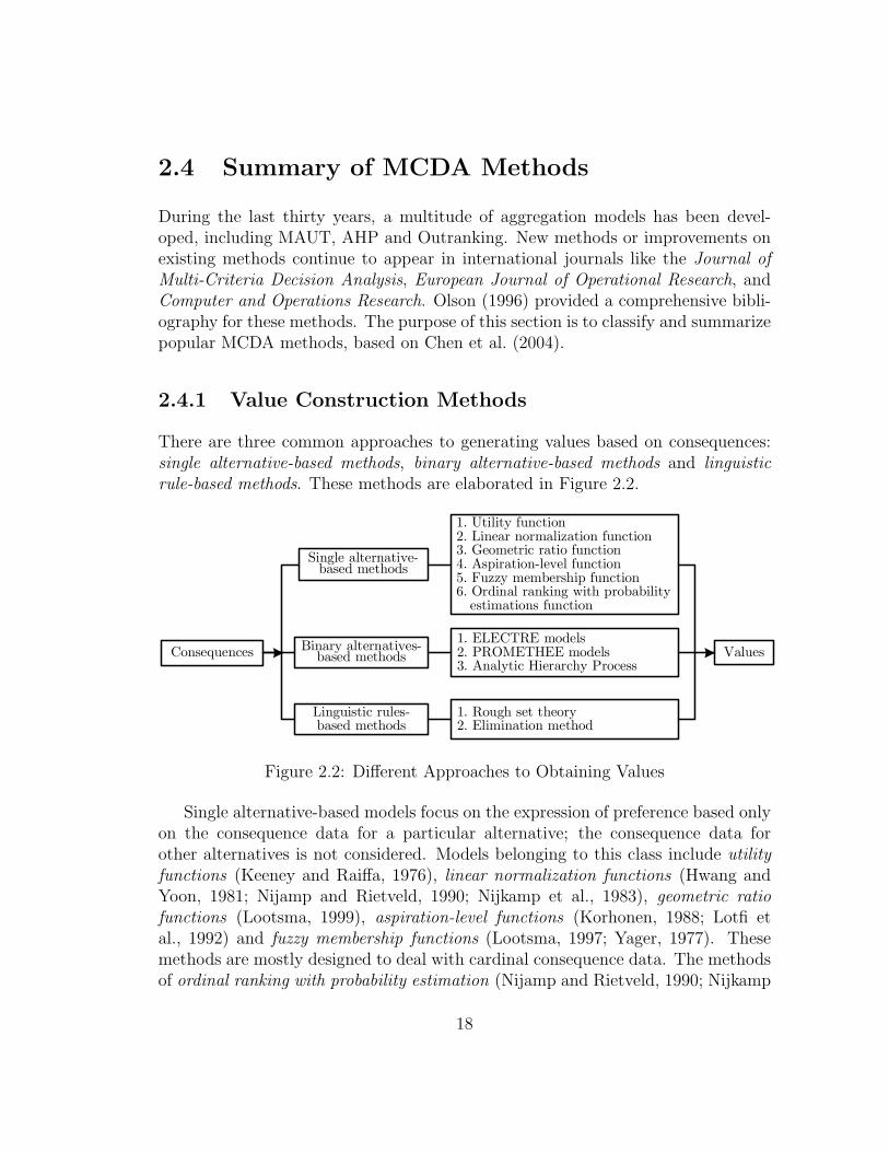
There are three common approaches to generating values based on consequences:single alternative-based methods, binary alternative-based methods and linguisticrule-based methods. These methods are elaborated in Figure 2.2.
Consequences
1. Utility function2. Linear normalization function3. Geometric ratio function4. Aspiration-level function5. Fuzzy membership function6. Ordinal ranking with probability estimations function
Single alternative-based methods
1. ELECTRE models2. PROMETHEE models3. Analytic Hierarchy Process
Binary alternatives-based methods
1. Rough set theory2. Elimination method
Linguistic rules-based methods
Values
Figure 2.2: Different Approaches to Obtaining Values
Single alternative-based models focus on the expression of preference based onlyon the consequence data for a particular alternative; the consequence data forother alternatives is not considered. Models belonging to this class include utilityfunctions (Keeney and Raiffa, 1976), linear normalization functions (Hwang andYoon, 1981; Nijamp and Rietveld, 1990; Nijkamp et al., 1983), geometric ratiofunctions (Lootsma, 1999), aspiration-level functions (Korhonen, 1988; Lotfi etal., 1992) and fuzzy membership functions (Lootsma, 1997; Yager, 1977). Thesemethods are mostly designed to deal with cardinal consequence data. The methodsof ordinal ranking with probability estimation (Nijamp and Rietveld, 1990; Nijkamp
18
et al., 1983) (since Nijkamp et al. (1983),and (Nijamp and Rietveld, 1990) did notgive a clear name for this method, in this document it is named according to itsmost distinguishing feature) and data envelopment analysis (Cook and Kress, 1991)apply to ordinal consequence data.
Most single alternative-based methods represent preferences using real numbers.In some methods, such as fuzzy membership, an interval of real numbers is obtainedfirst, and then aggregation methods are applied to obtain a single real number asrepresentative of this interval.
Binary relation-based models focus on expressions of preferences on criteriavia comparisons of two alternatives. They include ELECTRE (Roy, 1968, 1985),PROMETHEE (Brans et al., 1986; Brans and Vincke, 1985), and the AnalyticHierarchy Process (AHP) (Saaty, 1980). In AHP, binary relationships betweenalternatives are described by cardinal or ordinal numbers (usually relative scoreson a 1-9 scale), which represent the degree of preference between the alternatives,while in Outranking methods (ELECTRE or PROMETHEE) binary relations ofalternatives are represented by concordance and discordance matrices. Of course,difference exists between AHP and Outranking methods to obtain the final results.
Linguistic rules-based models focus on expressions of preferences on criteria viasome linguistic rules, mostly expressed as “If ..., then ...”. The advantage of thiskind of preference data is that people make decisions by searching for rules thatprovide good justification of their choices. Rough set methods (Slowinski, 1992)and the elimination method (MacCrimmon, 1973; Radford, 1989) are based on thiskind of preference representation.
2.4.2 Weighting Techniques
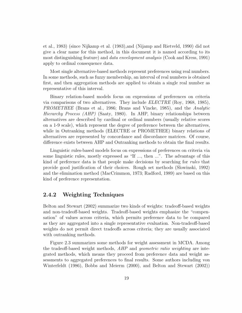
Belton and Stewart (2002) summarize two kinds of weights: tradeoff-based weightsand non-tradeoff-based weights. Tradeoff-based weights emphasize the “compen-sation” of values across criteria, which permits preference data to be comparedas they are aggregated into a single representative evaluation. Non-tradeoff-basedweights do not permit direct tradeoffs across criteria; they are usually associatedwith outranking methods.
Figure 2.3 summarizes some methods for weight assessment in MCDA. Amongthe tradeoff-based weight methods, AHP and geometric ratio weighting are inte-grated methods, which means they proceed from preference data and weight as-sessments to aggregated preferences to final results. Some authors including vonWinterfeldt (1986), Bobbs and Meierm (2000), and Belton and Stewart (2002))
19
Criteria
Tradeoff-based weights
Non-tradeoff-based weights
1. AHP2. Swing weights3. Geometric ratio weighting4. Ordinal ranking with probability estimations5. Data envelopment analysis
1. ELECTRE2. PROMETHEE
Figure 2.3: Methods of Weight Construction
prefer swing weights to other methods for direct estimation of weights. Ordinalranking with probability estimation was introduced by Nijkamp et al. (1983) to ex-press weights ordinally. Data envelopment analysis, proposed by Cook et al. (1996),possesses the unique feature that the values of weights are determined by prefer-ences to optimize the measure of each alternative. Note that Outranking methodsfocus on the employment of weights and do not provide procedures to obtain weightswhile other methods can generate the weight information.
2.4.3 Aggregation Methods
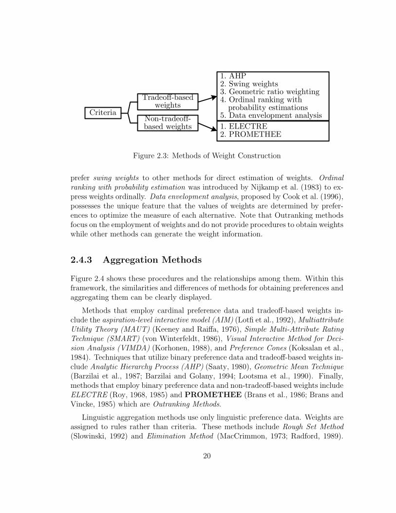
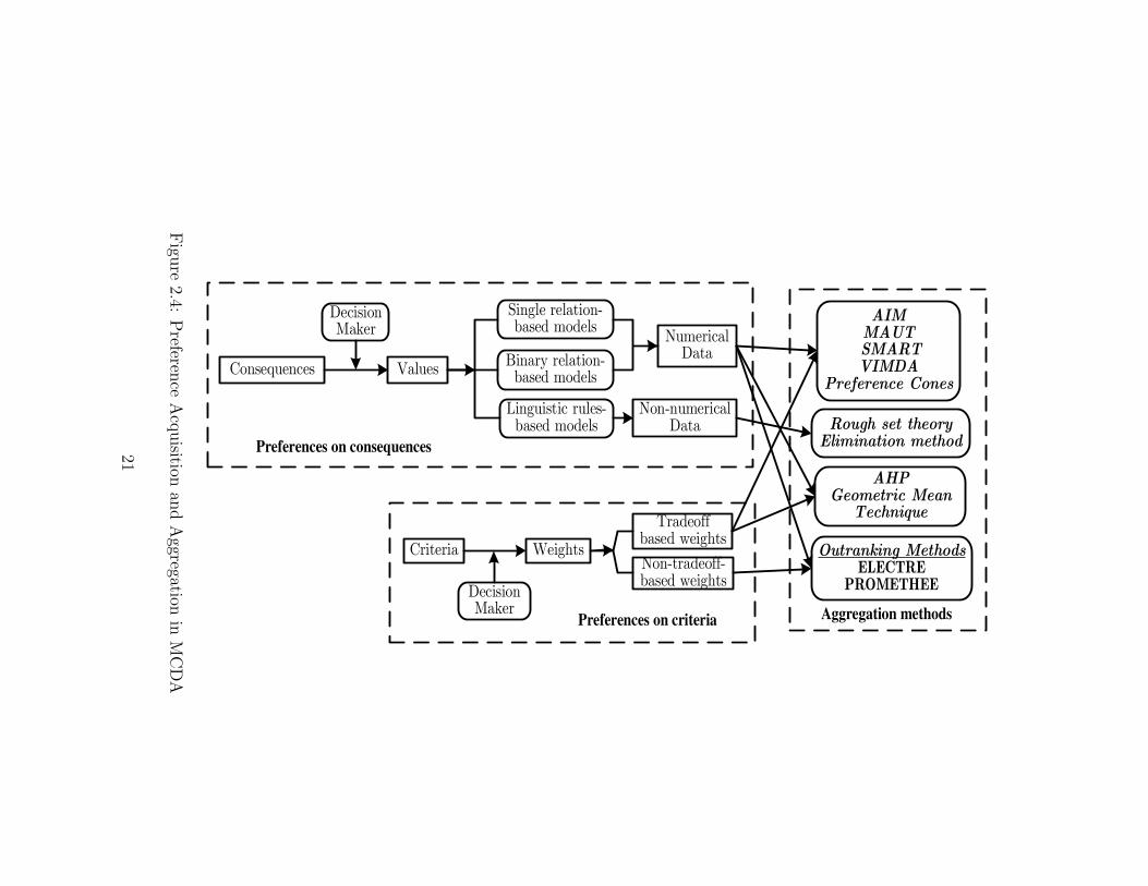
Figure 2.4 shows these procedures and the relationships among them. Within thisframework, the similarities and differences of methods for obtaining preferences andaggregating them can be clearly displayed.
Methods that employ cardinal preference data and tradeoff-based weights in-clude the aspiration-level interactive model (AIM) (Lotfi et al., 1992), MultiattributeUtility Theory (MAUT) (Keeney and Raiffa, 1976), Simple Multi-Attribute RatingTechnique (SMART) (von Winterfeldt, 1986), Visual Interactive Method for Deci-sion Analysis (VIMDA) (Korhonen, 1988), and Preference Cones (Koksalan et al.,1984). Techniques that utilize binary preference data and tradeoff-based weights in-clude Analytic Hierarchy Process (AHP) (Saaty, 1980), Geometric Mean Technique(Barzilai et al., 1987; Barzilai and Golany, 1994; Lootsma et al., 1990). Finally,methods that employ binary preference data and non-tradeoff-based weights includeELECTRE (Roy, 1968, 1985) and PROMETHEE (Brans et al., 1986; Brans andVincke, 1985) which are Outranking Methods.
Linguistic aggregation methods use only linguistic preference data. Weights areassigned to rules rather than criteria. These methods include Rough Set Method(Slowinski, 1992) and Elimination Method (MacCrimmon, 1973; Radford, 1989).
20
Criteria Weights
Decision Maker
Tradeoff based weights
Non-tradeoff-based weights
Consequences
Decision Maker
Values
Preferences on consequences
Preferences on criteria
AIMMAUTSMARTVIMDA
Preference Cones
AHPGeometric Mean
Technique
Outranking MethodsELECTRE
PROMETHEE
Aggregation methods
Single relation-based models
Rough set theoryElimination method
Numerical Data
Non-numerical Data
Linguistic rules-based models
Binary relation-based models
Figu
re2.4:
Preferen
ceA
cquisition
and
Aggregation
inM
CD
A
21
Greco et al. (2001) argue that “The rules explain the preferential attitude of thedecision maker and enable his/her understanding of the reasons of his/her prefer-ences.”
2.5 Conclusions
In this chapter, the basic context of MCDA is explained as follows:
• MCDA and relevant research topics: MCDA and its related research arediscussed and summarized in detail.
• Analysis procedures in MCDA: An analysis procedure for MCDA, conse-quence based preference aggregation, is explained in detail to establish ageneral framework for MCDA.
• Summary of methods in MCDA: Based upon the aforementioned analysis pro-cedure, many methods in MCDA are summarized and integrated into a sys-tematic framework to demonstrate the essence of these different approaches.
22
Chapter 3
Screening Problems in MultipleCriteria Decision Analysis
3.1 Introduction
In this chapter, screening problems are systematically addressed. Firstly a gen-eral description of screening problems is presented. Next, a sequential screeningprocedure is proposed to solve screening problem and the properties of sequentialscreening are discussed; then several popular MCDA methods are applied to screen-ing by using only partial decision information. Finally, the systematic use of thisprocedure is demonstrated in a case study of the Waterloo water supply planningin Southern Ontario, Canada. This Chapter is based on earlier research by Chenet al. (2005b).
3.2 General Description of Screening Problems
First a formal definition of screening for a decision problem in MCDA is presented.
Definition 3. A screening procedure is any procedure Scr that always selects anon-empty subset of an alternative set A,
∅ 6= Scr(A) ⊂ A, (3.1)
where Scr denotes a screening procedure (sometimes subscripts are used to dis-tinguish among different types of screening procedures), and Scr(A) denotes the
23
screened set (the remaining alternatives) after the procedure Scr was applied tothe alternative set A.
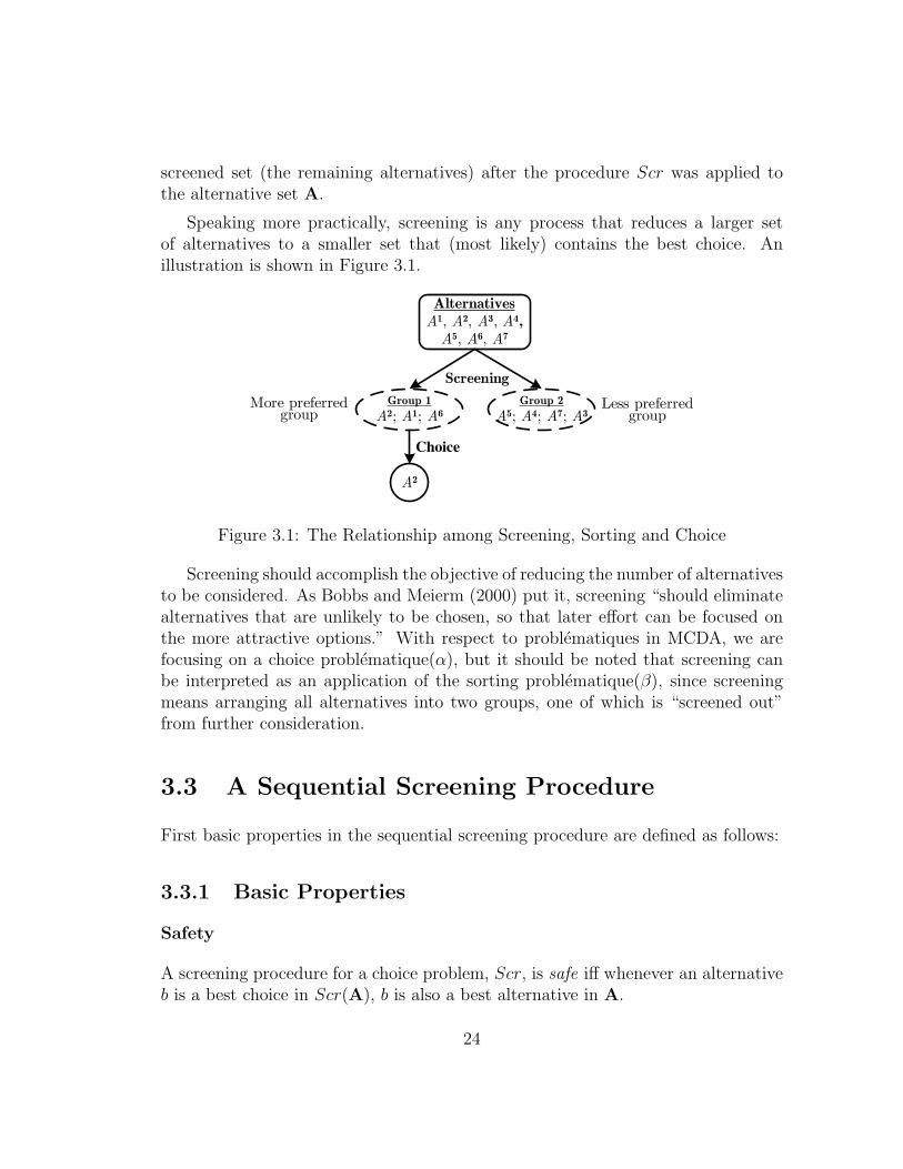
Speaking more practically, screening is any process that reduces a larger setof alternatives to a smaller set that (most likely) contains the best choice. Anillustration is shown in Figure 3.1.
Alternatives
A1, A2, A3, A4,
A5, A6, A7
A2
Group 1
A2; A1; A6
Group 2
A5; A4; A7; A3More preferred
groupLess preferred
group
Choice
Screening
Figure 3.1: The Relationship among Screening, Sorting and Choice
Screening should accomplish the objective of reducing the number of alternativesto be considered. As Bobbs and Meierm (2000) put it, screening “should eliminatealternatives that are unlikely to be chosen, so that later effort can be focused onthe more attractive options.” With respect to problematiques in MCDA, we arefocusing on a choice problematique(α), but it should be noted that screening canbe interpreted as an application of the sorting problematique(β), since screeningmeans arranging all alternatives into two groups, one of which is “screened out”from further consideration.
3.3 A Sequential Screening Procedure
First basic properties in the sequential screening procedure are defined as follows:
3.3.1 Basic Properties
Safety
A screening procedure for a choice problem, Scr, is safe iff whenever an alternativeb is a best choice in Scr(A), b is also a best alternative in A.
24
Efficiency
If Scr1 and Scr2 are distinct screening procedures, then Scr1 is more efficient thanScr2, or a refinement of Scr2, iff Scr1(A) ⊆ Scr2(A) is always true.
Information
In a screening procedure, information refers to preference information providedby the DM. For example, some aspects of the DM’s preference may be confirmedwithout providing complete information. Generally speaking, the more preferenceinformation included in a screening procedure, the more alternatives it can screenout. In the extreme case, information may be so strong that only one alternativeis left after screening.
Based on the description of consequences, values, weights and aggregation mod-els in Chapter 2, there are four types of screening information as follows:
• I1: the validation of basic preference properties;
• I2: the application of preference information on consequences;
• I3: the application of preference information on criteria;
• I4: the integration of aggregation models.
It is assumed that if Scr1 is a refinement of Scr2, then Scr1 is based on moreinformation than Scr2.
3.3.2 Sequential Screening
The DM may not be satisfied with the result of an initial screening. If so, otherscreening procedures may be applied to the screened set. Typically these follow-up procedures are based on more detailed preference information. This process iscalled sequential screening.
Definition 4. Sequential screening is the application of a series of screening pro-cedures in sequence to an alternative set A,
Scrh,h−1,...,1(A) = Scrh
(
Scrh−1
(
· · ·(
Scr1(A))
· · ·)
)
, (3.2)
25
where Scrk, k = 1, 2, ..., h are screening procedures. Scrh is the final screeningprocedure in this sequential screening.
Theorem 1. Sequential screening Scrh,h−1,...,1 is safe iff Scrk is safe for k =1, 2, · · · , h.
Proof: By hypothesis, Scr1 is safe. Now assume Scrk−1,k−2,...,1 is safe and considerScrk,k−1,...,1. Because Scrk is safe, a best alternative in Scrk,k−1,...,1(A) is a bestalternative in Scrk−1,k−2,...,1(A), which by assumption is a best alternative in A.Therefore, Theorem 1 is true by induction. ¤
3.3.3 Decision Information Based Screening
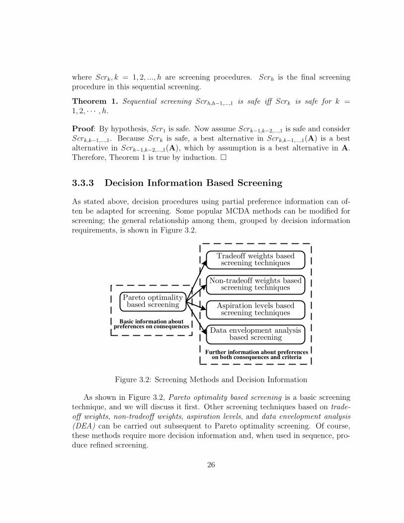
As stated above, decision procedures using partial preference information can of-ten be adapted for screening. Some popular MCDA methods can be modified forscreening; the general relationship among them, grouped by decision informationrequirements, is shown in Figure 3.2.
Pareto optimality based screening Aspiration levels based
screening techniques
Data envelopment analysis based screening
Non-tradeoff weights based screening techniques
Tradeoff weights based screening techniques
Basic information about preferences on consequences
Further information about preferences on both consequences and criteria
Figure 3.2: Screening Methods and Decision Information
As shown in Figure 3.2, Pareto optimality based screening is a basic screeningtechnique, and we will discuss it first. Other screening techniques based on trade-off weights, non-tradeoff weights, aspiration levels, and data envelopment analysis(DEA) can be carried out subsequent to Pareto optimality screening. Of course,these methods require more decision information and, when used in sequence, pro-duce refined screening.
26
3.3.4 Pareto Optimality (PO) Based Screening
Pareto optimality is a famous concept put forward by Pareto (1909) and is widelyused in economics and elsewhere. It provides a very useful definition of optimalityin MCDA because it can be interpreted to take account of multiple aspects (criteria)for overall optimality. Definitions of Pareto optimality in Multiple Objective Math-ematical Programming (MOMP) (Steuer, 1986) do not explain well the relationsbetween consequence data and preference data and are not suitable as screeningtechniques in MCDA. So we re-define the concept of Pareto optimality in MCDA.
Domination and Pareto Optimality
Domination is a relation that might or might not hold between two alternatives.
Definition 5. B ∈ A dominates A ∈ A, denoted B ≻ A, iff ∀j ∈ Q, vj(B) ≥ vj(A)with at least one strict inequality.
Using domination, we define Pareto optimality.
Definition 6. A ∈ A is a Pareto Optimal (PO) alternative, also called an efficientalternative, iff ∄ B ∈ A such that B ≻ A. The set of all Pareto optimal alternativesin A is denoted PO(A).
Usually, the information provided by the DM during the screening phrase islimited and the DM may prefer not to spend too much energy on comprehen-sive preference expressions. Then the following theorem shows that by identifyingPO(A), we carry out PO based direct screening in MCDA based on consequences,provided some properties of preference data hold.
Theorem 2. Assume the preference directions over criteria are available. A 6∈PO(A) iff ∃ B ∈ A such that ∀j ∈ Q, cj(A) ≤ cj(B) when j is a positive preferencecriterion and cj(A) ≥ cj(B) when j is a negative preference criterion, with at leastone strict inequality. For a choice problem, if A 6∈ PO(A), then A can be safelyscreened out.
Proof : Suppose that A ∈ A and ∃ B ∈ A such that ∀j ∈ Q, either cj(A) ≤ cj(B)and j is a positive preference criterion, or cj(A) ≥ cj(B) and j is negative preferencecriterion, with at least one strict inequality for some j ∈ Q. Taking into account theavailable information on preference directions over criteria, vj(A) ≤ vj(B) wheneverj is a positive preference criterion or a negative preference criterion. Therefore
27

∃ B ∈ A such that vj(A) ≤ vj(B) ∀j ∈ Q with at least one strict inequality.Therefore, according to Definition 5, B ≻ A and by Definition 6, A 6∈ PO(A). Thereverse implication is easy to verify directly.
As stated, the choice problem is to select the best alternative from A. If A /∈PO(A), then ∃B ≻ A. It is unknown whether B is the best alternative, but A canbe safely screened out since B is better than A, so that A cannot be best. ¤
Theorem 2 clarifies both the relation between preference data and consequencedata for the determination of Pareto optimality and the relation between Paretooptimality and screening for choice problems. We can safely use consequence datato screen out alternatives that are not Pareto optimal, as long as we are sure thebasic preference properties are satisfied.
Although many researchers had assumed the idea of Theorem 2 (checking Paretooptimality by consequence data), it is important to clarify the relation betweenPareto optimality in consequence data and preference data; otherwise improperscreening of alternatives may result.
PO Based Screening Procedure
• Identify preference direction (positive or negative) for each criterion;
• Compare alternatives based on their consequence data;
• Determine dominated alternatives based on Theorem 2;
• Remove dominated alternatives and retain non-dominated alternatives.
3.3.5 Tradeoff Weights (TW) Based Screening
PO based screening removes some alternatives. But DMs may not be satisfiedif many alternatives remain. Moreover, the power of PO based screening usuallydecreases as the number of criteria increases. Further information is needed in orderthat more efficient screening can be carried out.
TW based screening techniques are related to the research areas such as sensi-tivity analysis (Insua, 1990; Insua and French, 1991) and dominance and potentialoptimality (Athanassopoulos and Podinovski, 1997; Hazen, 1986). Although thesemethods focused on different questions, they all screen alternatives in choice prob-lems since they classify alternatives as either dominated (and therefore screened
28
out) or non-dominated. Here, we summarize these methods and put forward asystematic screening method, tradeoff weights (TW) based screening, that underliesthe existence of tradeoff weights.
Basic Concepts and Information Requirements
With TW based screening, the following further information from the DM is needed:
(1) The preference vector v(Ai) ∈ Rq, ∀Ai ∈ A.
(2) The final aggregation model.
Since most of these methods use a linear additive value function as the aggrega-tion model, we also adopt it. The linear additive value function model, introducedin (2.5), is given by
V (Ai) =⟨
v(Ai),w⟩
=∑
j∈Q
wj · vj(Ai)
where V (Ai) is the evaluation of alternative Ai and w is the weight vector.
Potential Optimality (PotOp) and Screening
Based on the linear additive value model, we define potential optimality and considerthe relationship between potential optimality and screening.
Definition 7. An alternative Ai ∈ A is potentially optimal (PotOp) iff there existsw such that
⟨
v(Ai),w⟩
= maxAk∈A
⟨
v(Ak),w⟩
. The set of all PotOp alternatives is
denoted as ScrPotOp(A) = PotOp(A) ⊆ A.
Theorem 3. Suppose Ai ∈ PotOp(A) and w ∈ W. If⟨
v(Ai),w⟩
≥⟨
v(Ak),w⟩
for all Ak ∈ PotOp(A), then⟨
v(Ai),w⟩
≥⟨
v(Ak),w⟩
∀Ak ∈ A.
Proof : Assume that⟨
v(Ai),w⟩
≥⟨
v(Ak),w⟩
for all Ak ∈ PotOp(A). If the the-orem fails, then there exists Aj /∈ PotOp(A) such that
⟨
v(Aj),w⟩
>⟨
v(Ai),w⟩
.Therefore, from Definition 7 there exists Ah ∈ PotOp(A) such that
⟨
v(Ah),w⟩
≥⟨
v(Ak),w⟩
for all Ak ∈ A. In particular,⟨
v(Ah),w⟩
≥⟨
v(Aj),w⟩
, andhence,
⟨
v(Ah),w⟩
>⟨
v(Ai),w⟩
, contradicting the hypothesis that⟨
v(Ai),w⟩
≥⟨
v(Ak),w⟩
for all Ak ∈ PotOp(A), which proves the theorem. ¤
From this theorem, it follows that if Ai is best with respect to w in PotOp(A),then Ai is best with respect to w in A. Therefore, PotOp screening is safe.
29
The following mathematical program can be used to determine whether alter-native Ai is potentially optimal (Geoffrion, 1968).
SCR.1(Ai) Minimize: δ
Subject to:⟨
w,(
v(Ai) − v(B))
⟩
+ δ ≥ 0, ∀ B ∈ A
w ∈ Wδ ≥ 0
The inputs of SCR.1(Ai) are v(Ai), v(B), and outputs are δ and w. If δ∗ = 0,then Ai ∈ PotOp(A). If δ∗ > 0, then Ai is not potentially optimal. Unlesscomputational considerations intervene, ScrPotOp can be implemented using thisprogram as the fundamental step.
TW Based Screening Procedure
• Check the validity of the linear additive preference function (SMART) as-sumption;
• Obtain the preference functions and get the preference data from the conse-quence data;
• For each Ai ∈ A, apply SCR.1(Ai) to identify PotOp(A);
• Retain only the potential optimal alternatives.
3.3.6 Non-tradeoff Weights (NTW) Based Screening
Since non-tradeoff weights based techniques belong to the family of outrankingmethods, they can also be called outranking based screening. Roy (1968) is con-sidered to have originated these methods.
Definition 8. Vincke (1992, p.58) An outranking relation is a binary relation Sdefined on A, with the interpretation that ASB if, given what is known about theDM’s preferences and values, the alternatives and the nature of the problem, thereare enough arguments to decide that A is at least as good as B, while there is noessential reason to refute that statement.
Many screening methods are based on an outranking relation.
Outranking methods are suitable for screening in MCDA, as Vincke (1992, p.57)notes: “Considering a choice problem, for example: if it is known that some action
30
(alternative) a is better than b and c, it becomes irrelevant to analyze preferencesbetween b and c. Those two actions can perfectly remain incomparable withoutendangering the decision-aid procedure.”
The major families of outranking methods are the ELECTRE methods and thePROME-THEE methods. ELECTRE I and PROMETHEE I are the best knownand most widely used methods within their respective families.
ELECTRE Technique for Screening
ELECTRE seeks to reduce the set of nondominated alternatives. The DM is askedto provide a set of weights reflecting relative importance (but they are not fortradeoffs purposes). Alternatives are eliminated if they are dominated by other al-ternatives to a specified degree defined by the DM. The system uses a concordanceindex to measure the relative advantage of an alternative over all other alterna-tives and a discordance index to measure its relative disadvantage. These indicesdetermine a dominated set, which is then screened out.
PROMETHEE Technique for Screening
PROMETHEE is an offshoot of ELECTRE. PROMETHEE methods begin with avalued outranking function, the outranking degree π(A,B), defined for each orderedpair of alternatives (A, B ∈ A × A, A 6= B). Hence π(A,B) represents a measureof how much better A is than B; 0 ≤ π(A,B) ≤ 1. For the details about the formof π(A,B), see Vincke (1992).
The overall outranking degree for alternative A is defined by the values of twofunctions: Φ+(A) (outgoing flow, which refers to the intensity of preference forA over other alternatives) and Φ−(A) (incoming flow, the intensity of preferencefor other alternatives relative to A). The definitions of Φ+(A) and Φ−(A) are asfollows:
Φ+(A) =∑
B∈A
π(A,B), (3.3)
Φ−(A) =∑
B∈A
π(B,A) (3.4)
The final step is the generation of the outranking relations over all alternatives.
Definition 9. AP+B iff Φ+(A) > Φ+(B); AP−B iff Φ−(A) < Φ−(B).
AI+B iff Φ+(A) = Φ+(B); AI−B iff Φ−(A) = Φ−(B).
31
A outranks B if 〈AP+B and AP−B〉 or 〈AP+B and AI−B〉 or 〈AI+B and AP−B〉.
All alternatives that are outranked by any alternative are then screened out.
3.3.7 Aspiration Levels (AL) Based Screening
Aspiration-level based screening techniques are techniques employing desired or ac-ceptable consequence levels of criteria to identify better alternatives (these methodsare also called reference point approaches (Hanne, 2001), but we prefer the name as-piration levels based screening, as proposed by Lotfi et al. (1992). Techniques suchas Goal Programming (Charnes and Cooper, 1961), Compromise Programming (Ze-leny, 1982) and the Reference Point Approach (Wierzbicki, 1982) can be regardedas the inspirations of aspiration-based screening. To introduce these methods, weclassify them into two categories, simple linguistic methods and distance-based mod-els.
Simple Linguistic Screening
Simple linguistic screening techniques use linguistic expressions on criteria as con-straints (standards), eliminating alternatives that do not satisfy these constraints.The advantage of this method is that expressions are simple and there are fewermodel parameters to specify. We can further classify constraints into lexicographicand conjunctive/disjunctive (Hwang and Yoon, 1981), or Elimination method (Mac-Crimmon, 1973).
• Lexicographic Constraints: Criteria are ranked in order of the relative im-portance. For each criterion, a constraint (goal) is set as a standard. Then allalternatives are examined, one at a time, to assess whether the first criterionis satisfied. All alternatives that fail are screened out. Then proceed to thesecond criterion, etc.
• Disjunctive and Conjunctive Constraints: Disjunctive/conjunctive con-straints express conditions involving more than one criterion. In conjunctiveform, characterized by “and”, all the constraints (goals) must be satisfied inorder for an alternative not to be screened. In disjunctive form, characterizedby “or”, any alternative can remain as long as it meets at least one of theconstraints. Conjunctive constraints are more powerful for screening since analternative must pass all the standards, so relatively few alternatives will suc-ceed unless the standards are set at a low level. In the disjunctive form, only
32
one standard must be met, so most alternatives will pass unless all standardsare set very high.
Distance-based Screening
Distance-based screening employs a measure of distance between an alternativeand some reference point (ideal alternative or aspiration level) as an index to screenout the alternatives that are too far away. Here we briefly introduce the aspiration-level interactive model (AIM) for screening, proposed by Lotfi et al. (1992).Its main steps are listed below.
Problem Definition: Three attainment levels for consequences must be estab-lished for each criterion j:
• The “want” level ASj expresses the aspiration level on each criterion;
• The “ideal” level (Ij) and “nadir” levels (Nj) express the largest and smallestconsequence data for each criterion.
Solution Process:
• Order the consequence data, {cj(A) : A ∈ A}, from least to most preferredfor each criterion j. Then inform the DM of the current aspiration level ASj
for each criterion, and the proportion of alternatives that achieve it;
• For every alternative, identify the “nearest nondominated alternative”, de-fined to be the closest alternative according to a scalarizing function proposedby Wierzbicki (1986) (see Lotfi et al. (1992) for more details) with the weighton criterion j given by wj = (ASj − Nj)/(Ij − Nj). The weights are setto reflect the increasing importance attached to criterion j as the aspirationlevel is moved closer to the ideal. Notice that these weights serve only fortemporary rankings and not any other purpose.
Screening Process: To screen alternatives, two options are available to the DM.
• First, the DM can reset one or several aspiration levels. This is useful whenthe DM is not sure about his aspiration level. Updated nearest nondominatedalternatives (perhaps the same, perhaps not) are obtained based on theseaspiration levels. Then only these nearest alternatives remain for furtherconsideration; all others are screened out.
33
• Second, if the DM prefers not to express aspiration levels, he or she canrequest a set of “neighboring” alternatives based on single aspiration levels.All alternatives other than these “neighboring” ones are then screened out.Lotfi et al. (1992) propose the use of ELECTRE-based outranking to find theneighbors of the nearest alternative.
3.3.8 Data Envelopment Analysis (DEA) Based Screening
Data Envelopment Analysis (DEA) is a technique used to measure the relativeefficiency of a number of similar units performing essentially the same task. DEAwas first put forward by Charnes et al. (1978) who proposed the basic DEA model,called CCR.
Within the past few decades, research into the relation between DEA andMCDA has carried out by authors including Belton and Vickers (1993), Stew-art (1996), Cook and Kress (1991), and Cook et al. (1996). Stewart comparedand contrasted the goals of DEA and MCDA: DEA arises from situations wherethe goal is to determine the productive efficiency of a system or ‘decision makingunit’ (DMU) by comparing how well the unit converts inputs into outputs, whileMCDA models have arisen from the need to analyze a set of alternatives accordingto conflicting criteria. A ‘methodological connection’ between MCDA and DEA isthat if all criteria in an MCDA problem can be classified as either benefit criteria(benefits or output) or cost criteria (costs or inputs), then DEA is equivalent toMCDA using additive linear value functions (Stewart, 1996).
The basic function of DEA is to ascertain which units are efficient and whichare not; in MCDA, these can be regarded as non-dominated and dominated al-ternatives, respectively. Cook and Kress (1991); Cook et al. (1996) applied someDEA-based models to deal with MCDA problems with both cardinal and ordinalcriteria. All dominated alternatives identified by the DEA-based model can bescreened out.
DEA Software: Frontier Analyst
Frontier Analyst is commercial software based on DEA theory to measure andimprove the performance of organizations. Below, Frontier Analyst is employed forexecuting DEA computations in an illustrative example.
34
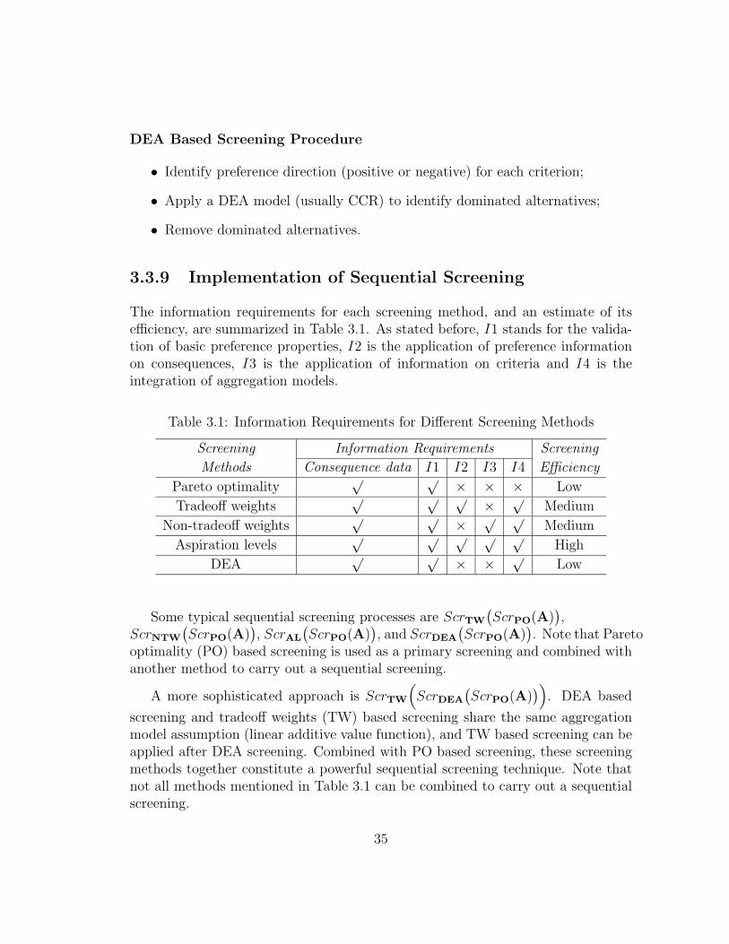
DEA Based Screening Procedure
• Identify preference direction (positive or negative) for each criterion;
• Apply a DEA model (usually CCR) to identify dominated alternatives;
• Remove dominated alternatives.
3.3.9 Implementation of Sequential Screening
The information requirements for each screening method, and an estimate of itsefficiency, are summarized in Table 3.1. As stated before, I1 stands for the valida-tion of basic preference properties, I2 is the application of preference informationon consequences, I3 is the application of information on criteria and I4 is theintegration of aggregation models.
Table 3.1: Information Requirements for Different Screening Methods
Screening Information Requirements Screening
Methods Consequence data I1 I2 I3 I4 Efficiency
Pareto optimality√ √ × × × Low
Tradeoff weights√ √ √ × √
Medium
Non-tradeoff weights√ √ × √ √
Medium
Aspiration levels√ √ √ √ √
High
DEA√ √ × × √
Low
Some typical sequential screening processes are ScrTW
(
ScrPO(A))
,ScrNTW
(
ScrPO(A))
, ScrAL
(
ScrPO(A))
, and ScrDEA
(
ScrPO(A))
. Note that Paretooptimality (PO) based screening is used as a primary screening and combined withanother method to carry out a sequential screening.
A more sophisticated approach is ScrTW
(
ScrDEA
(
ScrPO(A))
)
. DEA based
screening and tradeoff weights (TW) based screening share the same aggregationmodel assumption (linear additive value function), and TW based screening can beapplied after DEA screening. Combined with PO based screening, these screeningmethods together constitute a powerful sequential screening technique. Note thatnot all methods mentioned in Table 3.1 can be combined to carry out a sequentialscreening.
35

3.4 Case Study: Waterloo Water Supply Plan-
ning (WWSP)
The Regional Municipality of Waterloo, located in the southwestern part of On-tario, Canada, comprises the three cities of Kitchener, Waterloo, and Cambridge,plus adjacent rural municipalities. At present, the Waterloo region is one of thelargest communities in Canada to rely almost exclusively on groundwater for itswater supply. Due to increases in residential, industrial and commercial demandand decreases in the reliability of groundwater resources, the Regional Governmentdeveloped over 1991-2000 a Long Term Water Strategy to the year 2041 (Rajabi,1997; Waterloo Regional Council, 2000).
The overall purpose of this project was to design and implement the best waterresources plan for the Waterloo Region. In light of this purpose, seven criteriawere proposed to evaluate possible alternatives. The detailed meanings of the cri-teria are as follows: INVEST: project investment cost (millions of dollars); OPER:project operating cost (millions of dollars); INFRA: project negative infrastruc-ture impact (0-100, greater values mean more negative impact); ENVIR: projectnegative environmental impact (0-100, greater values mean more negative impact);RISK: project implementation risk (0-100, greater values mean higher risk); SUP-PLY: project supply capability (million imperial gallons per day, MIGD); QUAL:the quality of the water the project will deliver (0-100, greater values mean higherwater quality). INFRA, ENVIR, RISK and QUAL are qualitative criteria; scoreswere assessed by the authors based on a report by Associated Engineering (1994).
Twelve alternatives were identified. Table 3.2 shows the MCDA problem con-stituted to represent the WWSP. The consequence data for water quality, envi-ronmental impacts and risk were estimated according to a preliminary evaluationby Associated Engineering (1994). SUPPLY and QUAL are identified as positivepreference criteria (indicated by “+” in Table 2); others are negative preferencecriteria (indicated by “-” in Table 2).
Below is a brief explanation of each of the twelve alternatives.
• Groundwater, option 1 (GW1) - Develop additional groundwater sources inthe vicinity of Kitchener-Waterloo.
• Groundwater, option 2 (GW2) - Develop groundwater sources in new fields,mainly in the south Woolwich area, the Roseville area, and the St. Agathaarea.
36
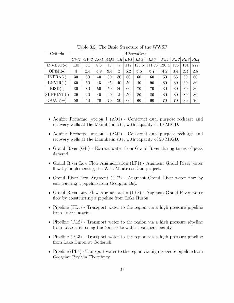
Table 3.2: The Basic Structure of the WWSP
Criteria Alternatives
GW1 GW2 AQ1 AQ2 GR LF1 LF2 LF3 PL1 PL2 PL3 PL4
INVEST(-) 100 61 8.6 17 5 112 123.6 111.25 120.4 126 181 222
OPER(-) 4 2.4 5.9 8.8 2 6.2 6.6 6.7 4.2 3.4 2.3 2.5
INFRA(-) 30 30 40 50 30 60 60 60 60 65 60 60
ENVIR(-) 60 60 45 45 40 50 40 90 80 80 80 80
RISK(-) 80 80 50 50 80 60 70 70 30 30 30 30
SUPPLY(+) 29 20 40 40 5 50 80 80 80 80 80 80
QUAL(+) 50 50 70 70 30 60 60 60 70 70 80 70
• Aquifer Recharge, option 1 (AQ1) - Construct dual purpose recharge andrecovery wells at the Mannheim site, with capacity of 10 MIGD.
• Aquifer Recharge, option 2 (AQ2) - Construct dual purpose recharge andrecovery wells at the Mannheim site, with capacity of 20 MIGD.
• Grand River (GR) - Extract water from Grand River during times of peakdemand.
• Grand River Low Flow Augmentation (LF1) - Augment Grand River waterflow by implementing the West Montrose Dam project.
• Grand River Low Augment (LF2) - Augment Grand River water flow byconstructing a pipeline from Georgian Bay.
• Grand River Low Flow Augmentation (LF3) - Augment Grand River waterflow by constructing a pipeline from Lake Huron.
• Pipeline (PL1) - Transport water to the region via a high pressure pipelinefrom Lake Ontario.
• Pipeline (PL2) - Transport water to the region via a high pressure pipelinefrom Lake Erie, using the Nanticoke water treatment facility.
• Pipeline (PL3) - Transport water to the region via a high pressure pipelinefrom Lake Huron at Goderich.
• Pipeline (PL4) - Transport water to the region via high pressure pipeline fromGeorgian Bay via Thornbury.
37
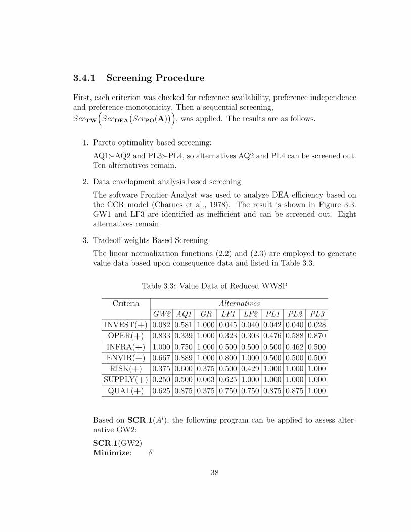
3.4.1 Screening Procedure
First, each criterion was checked for reference availability, preference independenceand preference monotonicity. Then a sequential screening,
ScrTW
(
ScrDEA
(
ScrPO(A))
)
, was applied. The results are as follows.
1. Pareto optimality based screening:
AQ1≻AQ2 and PL3≻PL4, so alternatives AQ2 and PL4 can be screened out.Ten alternatives remain.
2. Data envelopment analysis based screening
The software Frontier Analyst was used to analyze DEA efficiency based onthe CCR model (Charnes et al., 1978). The result is shown in Figure 3.3.GW1 and LF3 are identified as inefficient and can be screened out. Eightalternatives remain.
3. Tradeoff weights Based Screening
The linear normalization functions (2.2) and (2.3) are employed to generatevalue data based upon consequence data and listed in Table 3.3.
Table 3.3: Value Data of Reduced WWSP
Criteria Alternatives
GW2 AQ1 GR LF1 LF2 PL1 PL2 PL3
INVEST(+) 0.082 0.581 1.000 0.045 0.040 0.042 0.040 0.028
OPER(+) 0.833 0.339 1.000 0.323 0.303 0.476 0.588 0.870
INFRA(+) 1.000 0.750 1.000 0.500 0.500 0.500 0.462 0.500
ENVIR(+) 0.667 0.889 1.000 0.800 1.000 0.500 0.500 0.500
RISK(+) 0.375 0.600 0.375 0.500 0.429 1.000 1.000 1.000
SUPPLY(+) 0.250 0.500 0.063 0.625 1.000 1.000 1.000 1.000
QUAL(+) 0.625 0.875 0.375 0.750 0.750 0.875 0.875 1.000
Based on SCR.1(Ai), the following program can be applied to assess alter-native GW2:
SCR.1(GW2)Minimize: δ
38
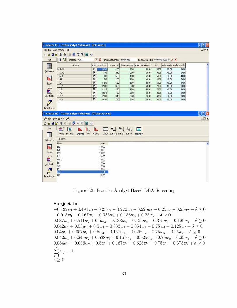
Figure 3.3: Frontier Analyst Based DEA Screening
Subject to:−0.499w1 + 0.494w2 + 0.25w3 − 0.222w4 − 0.225w5 − 0.25w6 − 0.25w7 + δ ≥ 0−0.918w1 − 0.167w2 − 0.333w4 + 0.188w6 + 0.25w7 + δ ≥ 00.037w1 + 0.511w2 + 0.5w3 − 0.133w4 − 0.125w5 − 0.375w6 − 0.125w7 + δ ≥ 00.042w1 + 0.53w2 + 0.5w3 − 0.333w4 − 0.054w5 − 0.75w6 − 0.125w7 + δ ≥ 00.04w1 + 0.357w2 + 0.5w3 + 0.167w4 − 0.625w5 − 0.75w6 − 0.25w7 + δ ≥ 00.042w1 + 0.245w2 + 0.538w3 + 0.167w4 − 0.625w5 − 0.75w6 − 0.25w7 + δ ≥ 00.054w1 − 0.036w2 + 0.5w3 + 0.167w4 − 0.625w5 − 0.75w6 − 0.375w7 + δ ≥ 07
∑
j=1
wj = 1
δ ≥ 0
39
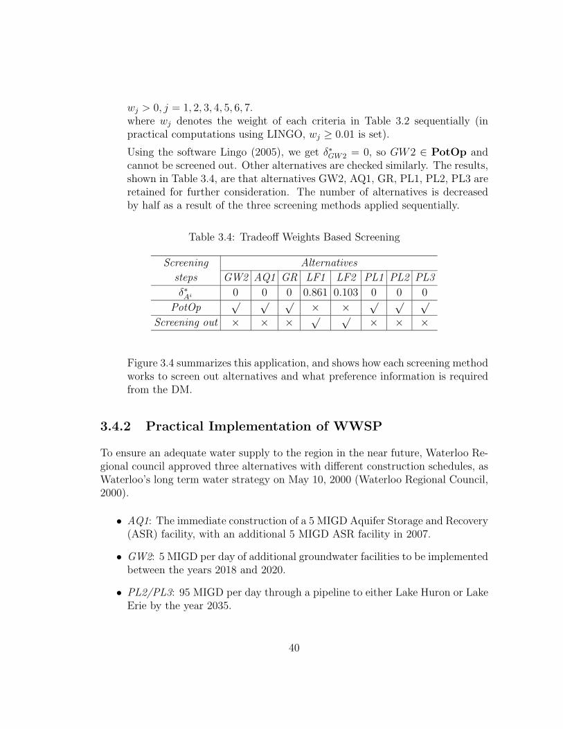
wj > 0, j = 1, 2, 3, 4, 5, 6, 7.where wj denotes the weight of each criteria in Table 3.2 sequentially (inpractical computations using LINGO, wj ≥ 0.01 is set).
Using the software Lingo (2005), we get δ∗GW2 = 0, so GW2 ∈ PotOp andcannot be screened out. Other alternatives are checked similarly. The results,shown in Table 3.4, are that alternatives GW2, AQ1, GR, PL1, PL2, PL3 areretained for further consideration. The number of alternatives is decreasedby half as a result of the three screening methods applied sequentially.
Table 3.4: Tradeoff Weights Based Screening
Screening Alternatives
steps GW2 AQ1 GR LF1 LF2 PL1 PL2 PL3
δ∗Ai 0 0 0 0.861 0.103 0 0 0
PotOp√ √ √ × × √ √ √
Screening out × × × √ √ × × ×
Figure 3.4 summarizes this application, and shows how each screening methodworks to screen out alternatives and what preference information is requiredfrom the DM.
3.4.2 Practical Implementation of WWSP
To ensure an adequate water supply to the region in the near future, Waterloo Re-gional council approved three alternatives with different construction schedules, asWaterloo’s long term water strategy on May 10, 2000 (Waterloo Regional Council,2000).
• AQ1: The immediate construction of a 5 MIGD Aquifer Storage and Recovery(ASR) facility, with an additional 5 MIGD ASR facility in 2007.
• GW2: 5 MIGD per day of additional groundwater facilities to be implementedbetween the years 2018 and 2020.
• PL2/PL3: 95 MIGD per day through a pipeline to either Lake Huron or LakeErie by the year 2035.
40
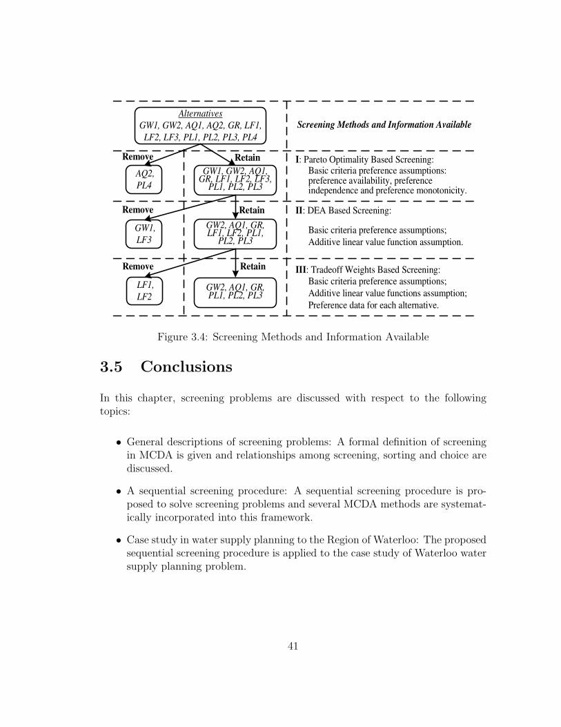
Alternatives
GW1, GW2, AQ1, AQ2, GR, LF1,
LF2, LF3, PL1, PL2, PL3, PL4
RetainRemove
AQ2,
PL4
GW1, GW2, AQ1, GR, LF1, LF2, LF3,
PL1, PL2, PL3
GW1,
LF3
GW2, AQ1, GR, LF1, LF2, PL1,
PL2, PL3
LF1,
LF2GW2, AQ1, GR, PL1, PL2, PL3
Screening Methods and Information Available
I: Pareto Optimality Based Screening:Basic criteria preference assumptions: preference availability, preference independence and preference monotonicity.
II: DEA Based Screening:
Basic criteria preference assumptions;
Additive linear value function assumption.
III: Tradeoff Weights Based Screening:
Basic criteria preference assumptions;
Additive linear value functions assumption;
Preference data for each alternative.
Remove
Remove
Retain
Retain
Figure 3.4: Screening Methods and Information Available
3.5 Conclusions
In this chapter, screening problems are discussed with respect to the followingtopics:
• General descriptions of screening problems: A formal definition of screeningin MCDA is given and relationships among screening, sorting and choice arediscussed.
• A sequential screening procedure: A sequential screening procedure is pro-posed to solve screening problems and several MCDA methods are systemat-ically incorporated into this framework.
• Case study in water supply planning to the Region of Waterloo: The proposedsequential screening procedure is applied to the case study of Waterloo watersupply planning problem.
41
Chapter 4
A Case-based Distance Methodfor Screening
4.1 Introduction
A case-based distance method for screening is proposed to solve screening prob-lems. Firstly, research underlying case-based reasoning in MCDA is summarized.Then, the assumptions of the proposed case-based distance method are explainedin detail. Subsequently, a quadratic program is constructed to find the best de-scriptive criterion weights and the screening thresholds. Based on this information,a procedure for carrying out a distance-based method for screening is proposed anda numerical example is utilized to demonstrate the proposed method. This chapterconstitutes an expanded version of the research of Chen et al. (2005c).
4.2 Case-based Reasoning
The main difficulty in the application of many MCDA methods lies in the acquisi-tion of the DM’s preference information in the form of values or weights. Case-basedreasoning is an approach to obtain preferential information from the DM’s decisionson selected cases, as for example in UTilites Additives (UTA) (Jacquet-Lagreze andSiskos, 1982) or rough set theory (Slowinski and Zopounidis, 1995). The test set ofcases may include:
• Past decisions taken by the DM;
42
• Decisions taken for a limited set of fictitious but realistic alternatives;
• Decisions taken for a representative subset of the alternatives under consider-ation, which are sufficiently familiar to the DM that they are easy to evaluate.
The advantages of case-based information include that “decision makers mayprefer to make exemplary decisions than to explain them in terms of specific func-tional model parameters” (Doumpos and Zopouidis, 2002). Meanwhile, some as-sumptions typical of functional models, for example preference monotonicity andpreference independence, can be relaxed, simplifying the process of criterion con-struction. Here, we propose a case-based distance model for screening. Followingthe general concept of the aggregation-disaggregation approach to MCDA (Jacquet-Lagreze and Siskos, 2001), we propose a specific case-based distance model forscreening.
4.3 Model Assumptions
4.3.1 Case Set Assumptions
Assume a test set of alternatives T. The alternatives in T may be, for example,fabricated by the DM or obtained by having the DM modify historical records.However all criteria in Q must apply and cj(A) must be measurable for all A ∈T and all j ∈ Q. Suppose that the DM specifies that all alternatives in Z ={z1, z2, ..., zr, ..., zm} ⊆ T are acceptable for a choice problem. Let | T |= t andlet T − Z = {zm+1, zm+2, ..., zp, ..., zt} denote the unacceptable cases.
The idea of our model is that based on the “right” distance concept, the casesin Z should be close together, and the cases in T − Z should be “outside” Z insome sense. We use T and Z to estimate criterion weights w, and a basic distancethreshold R ∈ R+, so that the distance of zr ∈ Z from the “center” of Z is lessor equal to R, and the distance of zp 6∈ Z from this “center” is greater than R.Then we can apply w and S (S = kR, where k ∈ R+ is a controllable distancethreshold for the DM) to screen out all “extreme” alternatives in A, and therebyobtain Scr(A). Figure 4.1 portrays this idea.
Given the acceptable case set Z, z, the centroid of Z is deemed to be a fictitiousalternative at the center of Z. By definition,
cj
(
z)
=1
m
m∑
r=1
cj
(
zr)
. (4.1)
43
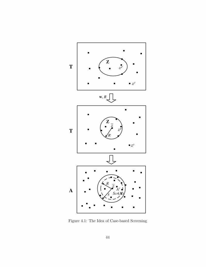
.
.
.
.
.
z
Z
.
.
.
.
.
z p
w, R
.
.
.
.
.
.
.
. Ai
.
R
.
.
.
.
.
. z
ZT
..
..
.
z p
.
.
.
.
.
.
.
.
.
A
.
.
. .
.
.
.
.
.
.
.
.
.
.
.
. .
.
.
.
.
.
..
Scr(A)s
T
.
_z
_z
R
.
.
Figure 4.1: The Idea of Case-based Screening
44

Recall that |Z| = m. Note that we assume that Z has the property that, for anycriterion j, not all values of cj(z
r) are equal.
4.3.2 Distance Assumptions
For j = 1, 2, ..., q, define dmaxj = max
r=1,2,...,m
(
cj(zr) − cj(z)
)2to be the normalization
factor for criterion j. The distance between zr ∈ Z and the centroid z on criterionj is
dj(zr, z) =
(
cj(zr) − cj(z)
)2
dmaxj
. (4.2)
Similarly, the distance between alternative Ai ∈ A and the centroid z on criterionj is
dj(Ai, z) =
(
cij − cj(z)
)2
dmaxj
. (4.3)
Note that (4.3) applies if Ai = zp ∈ {T−Z}, and 0 < dj(zr, z) ≤ 1 for zr ∈ Z, but
dj(zp, z) or dj(A
i, z) could be larger than 1.
Weighted Euclidean distance has a clear geometric meaning, which can be eas-ily understood and accepted to represent a DM’s aggregated preference. Insteadof weighted Euclidean distances, we use their squares, because they are easier tocompute while preserving order.
The distance between alternative zr ∈ Z and the case set Z is therefore identifiedwith the distance between zr and z, which is
D(zr) = D(zr, z) =∑
j∈Q
wj · dj(zr, z),
where wj ∈ w is the weight (relative importance) of criterion j. The weight vectorw is to be determined. The weights must satisfy 0 < wj ≤ 1, and
∑
j∈Q
wj = 1.
The distance of alternative Ai from the case set Z is
D(Ai) = D(Ai, z) =∑
j∈Q
wj · dj(Ai, z). (4.4)
Note that (4.4) applies if Ai = zp ∈ {T − Z}. The distance of an alternativefrom the case set is thus defined to be the distance between the alternative and thecentroid of the case set. A similar idea has been widely used in cluster analysis:
45
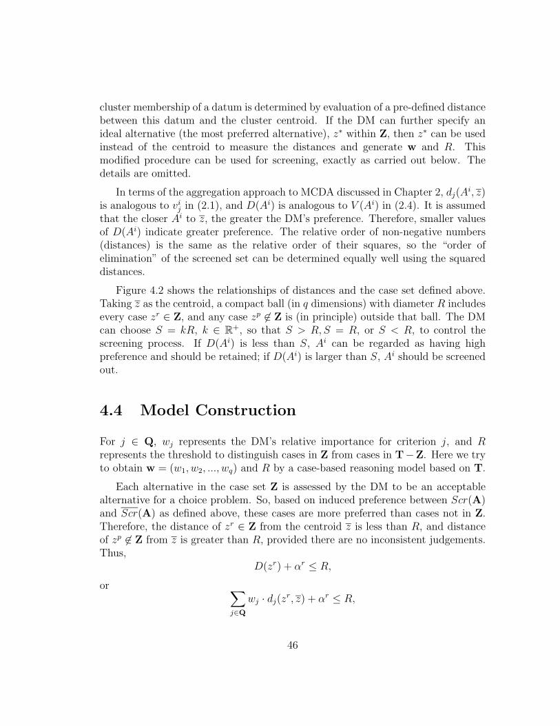
cluster membership of a datum is determined by evaluation of a pre-defined distancebetween this datum and the cluster centroid. If the DM can further specify anideal alternative (the most preferred alternative), z∗ within Z, then z∗ can be usedinstead of the centroid to measure the distances and generate w and R. Thismodified procedure can be used for screening, exactly as carried out below. Thedetails are omitted.
In terms of the aggregation approach to MCDA discussed in Chapter 2, dj(Ai, z)
is analogous to vij in (2.1), and D(Ai) is analogous to V (Ai) in (2.4). It is assumed
that the closer Ai to z, the greater the DM’s preference. Therefore, smaller valuesof D(Ai) indicate greater preference. The relative order of non-negative numbers(distances) is the same as the relative order of their squares, so the “order ofelimination” of the screened set can be determined equally well using the squareddistances.
Figure 4.2 shows the relationships of distances and the case set defined above.Taking z as the centroid, a compact ball (in q dimensions) with diameter R includesevery case zr ∈ Z, and any case zp 6∈ Z is (in principle) outside that ball. The DMcan choose S = kR, k ∈ R+, so that S > R, S = R, or S < R, to control thescreening process. If D(Ai) is less than S, Ai can be regarded as having highpreference and should be retained; if D(Ai) is larger than S, Ai should be screenedout.
4.4 Model Construction
For j ∈ Q, wj represents the DM’s relative importance for criterion j, and Rrepresents the threshold to distinguish cases in Z from cases in T−Z. Here we tryto obtain w = (w1, w2, ..., wq) and R by a case-based reasoning model based on T.
Each alternative in the case set Z is assessed by the DM to be an acceptablealternative for a choice problem. So, based on induced preference between Scr(A)and Scr(A) as defined above, these cases are more preferred than cases not in Z.Therefore, the distance of zr ∈ Z from the centroid z is less than R, and distanceof zp 6∈ Z from z is greater than R, provided there are no inconsistent judgements.Thus,
D(zr) + αr ≤ R,
or∑
j∈Q
wj · dj(zr, z) + αr ≤ R,
46
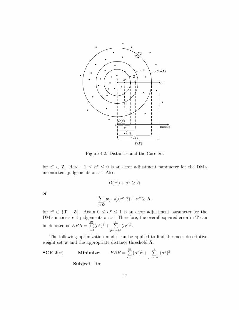
.
.
.
.
..
z
Z
.
rD(z )
z
D( )z
T
.
Scr(A)
D(Ai)
.
.
R
.
Distance
_z
..
.
.
0
S = kR
Ai
.
.
.
.
.
.
.
.
.
.
.
.
.
.
.
..
.
.
.
.
.
.
Figure 4.2: Distances and the Case Set
for zr ∈ Z. Here −1 ≤ αr ≤ 0 is an error adjustment parameter for the DM’sinconsistent judgements on zr. Also
D(zp) + αp ≥ R,
or∑
j∈Q
wj · dj(zp, z) + αp ≥ R,
for zp ∈ {T − Z}. Again 0 ≤ αp ≤ 1 is an error adjustment parameter for theDM’s inconsistent judgements on zp. Therefore, the overall squared error in T can
be denoted as ERR =m∑
r=1
(αr)2 +t
∑
p=m+1
(αp)2.
The following optimization model can be applied to find the most descriptiveweight set w and the appropriate distance threshold R.
SCR.2(α) Minimize: ERR =m∑
r=1
(αr)2 +t
∑
p=m+1
(αp)2
Subject to:
47

∑
j∈Q
wj · dj(zr, z) + αr ≤ R, r = 1, 2, ...,m;
∑
j∈Q
wj · dj(zp, z) + αp ≥ R, p = m + 1,m + 2, ..., t;
0 < R ≤ 1;
wj > 0, j = 1, 2, ..., q∑
j∈Q
wj = 1;
−1 ≤ αr ≤ 0, r = 1, 2, ...,m;
0 ≤ αp ≤ 1, p = m + 1,m + 2, ..., t.
Note that optimization software such as Lingo (Lingo, 2005) automatically con-verts strict inequalities in constraints, like wj > 0, to weak inequalities, like wj ≥ ǫ,where ǫ is small positive number generated internally when optimization is carriedout as in SCR.2(α). Here, we retain zero in the constraints for easy understand-ing of the program. Similar settings are applied to the other optimization modelsaddressed in the later chapters.
Theorem 4. SCR.2(α) has at least one optimal solution, w∗ and R∗.
Proof: The set of w satisfying the constraints in SCR.2(α) is bounded. The
objective function ERR =m∑
r=1
(αr)2 +t
∑
p=m+1
(αp)2 is a quadratic function on this
set. Based on the extreme value theorem of advanced calculus (Fitzpatrick, 1995,page 297), the function ERR is continuous and the set of all possible variables isbounded, ERR attains its minimum at least once. ¤
Two threshold parameters can be set by the DM to evaluate the errors generatedby SCR.2(α):
• The acceptable distance threshold, ∆D: ∆D is the threshold below whicherror generated by SCR.2(α) is acceptable to the DM (Note that ∆D shouldbe larger than ε∗). If ε∗ ≤ ERR∗ ≤ ∆D, the errors still are acceptable;otherwise T should be reset. A suggested value of ∆D is 1
10t, where |T| = t.
• The indifference threshold (see Vincke (1992) for detailed discussion of in-difference thresholds in MCDA), ε: ε is the threshold below which errorsgenerated by SCR.2(α) can be ignored. When ERR∗ ≤ ε, the case set Tand Z are consistent; but when ERR∗ ≥ ε, the errors cannot be ignored andthere is some inconsistency in T. A value suggested for ε is 1
10n, where n = |A|
is the number of alternatives in A. Of course,the DM can adjust the settingto keep the balance between indifference threshold and acceptable threshold.
48
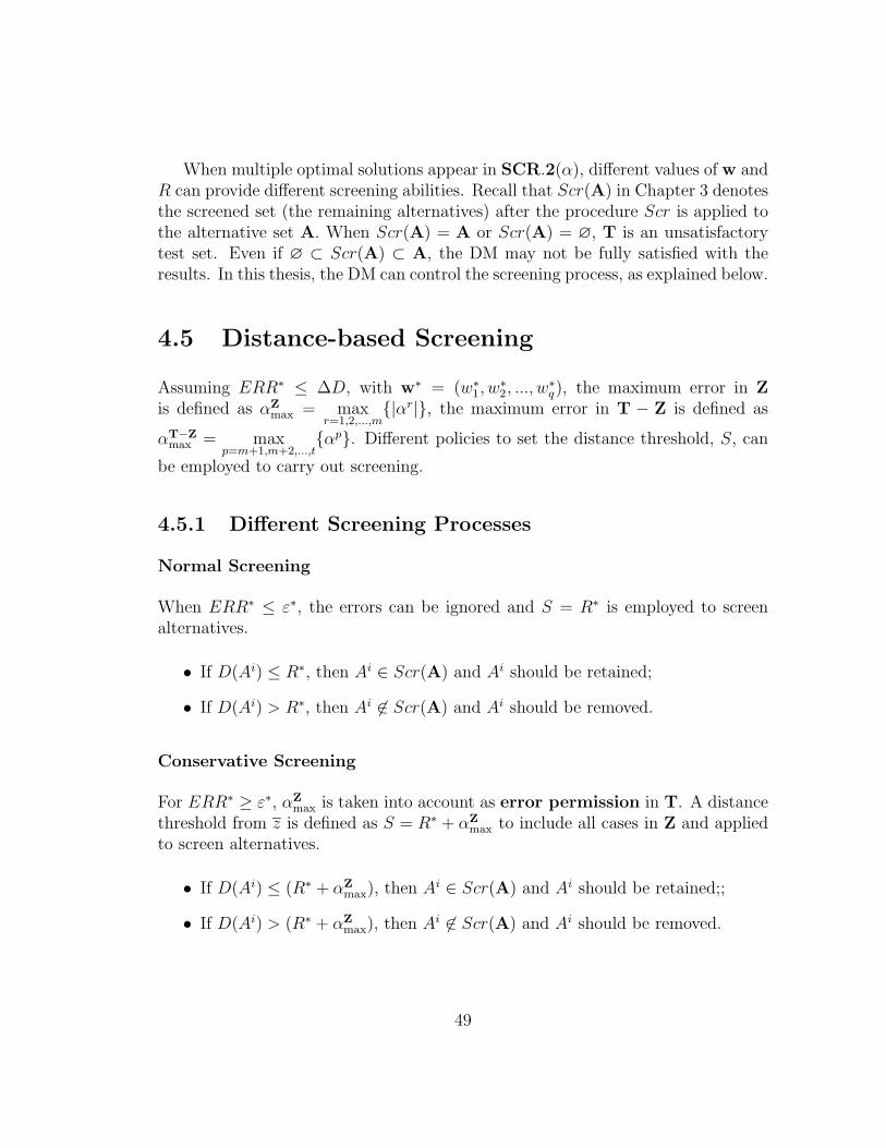
When multiple optimal solutions appear in SCR.2(α), different values of w andR can provide different screening abilities. Recall that Scr(A) in Chapter 3 denotesthe screened set (the remaining alternatives) after the procedure Scr is applied tothe alternative set A. When Scr(A) = A or Scr(A) = ∅, T is an unsatisfactorytest set. Even if ∅ ⊂ Scr(A) ⊂ A, the DM may not be fully satisfied with theresults. In this thesis, the DM can control the screening process, as explained below.
4.5 Distance-based Screening
Assuming ERR∗ ≤ ∆D, with w∗ = (w∗1, w
∗2, ..., w
∗q), the maximum error in Z
is defined as αZmax = max
r=1,2,...,m{|αr|}, the maximum error in T − Z is defined as
αT−Zmax = max
p=m+1,m+2,...,t{αp}. Different policies to set the distance threshold, S, can
be employed to carry out screening.
4.5.1 Different Screening Processes
Normal Screening
When ERR∗ ≤ ε∗, the errors can be ignored and S = R∗ is employed to screenalternatives.
• If D(Ai) ≤ R∗, then Ai ∈ Scr(A) and Ai should be retained;
• If D(Ai) > R∗, then Ai 6∈ Scr(A) and Ai should be removed.
Conservative Screening
For ERR∗ ≥ ε∗, αZmax is taken into account as error permission in T. A distance
threshold from z is defined as S = R∗ + αZmax to include all cases in Z and applied
to screen alternatives.
• If D(Ai) ≤ (R∗ + αZmax), then Ai ∈ Scr(A) and Ai should be retained;;
• If D(Ai) > (R∗ + αZmax), then Ai 6∈ Scr(A) and Ai should be removed.
49
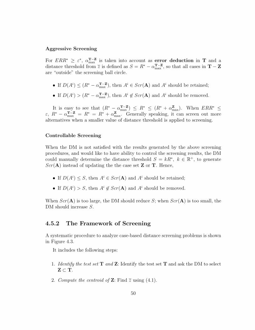
Aggressive Screening
For ERR∗ ≥ ε∗, αT−Zmax is taken into account as error deduction in T and a
distance threshold from z is defined as S = R∗ − αT−Zmax , so that all cases in T − Z
are “outside” the screening ball circle.
• If D(Ai) ≤ (R∗ − αT−Zmax ), then Ai ∈ Scr(A) and Ai should be retained;
• If D(Ai) > (R∗ − αT−Zmax ), then Ai 6∈ Scr(A) and Ai should be removed.
It is easy to see that (R∗ − αT−Zmax ) ≤ R∗ ≤ (R∗ + αZ
max). When ERR∗ ≤ε, R∗ − αT−Z
max = R∗ = R∗ + αZmax. Generally speaking, it can screen out more
alternatives when a smaller value of distance threshold is applied to screening.
Controllable Screening
When the DM is not satisfied with the results generated by the above screeningprocedures, and would like to have ability to control the screening results, the DMcould manually determine the distance threshold S = kR∗, k ∈ R+, to generateScr(A) instead of updating the the case set Z or T. Hence,
• If D(Ai) ≤ S, then Ai ∈ Scr(A) and Ai should be retained;
• If D(Ai) > S, then Ai 6∈ Scr(A) and Ai should be removed.
When Scr(A) is too large, the DM should reduce S; when Scr(A) is too small, theDM should increase S.
4.5.2 The Framework of Screening
A systematic procedure to analyze case-based distance screening problems is shownin Figure 4.3.
It includes the following steps:
1. Identify the test set T and Z: Identify the test set T and ask the DM to selectZ ⊂ T.
2. Compute the centroid of Z: Find z using (4.1).
50
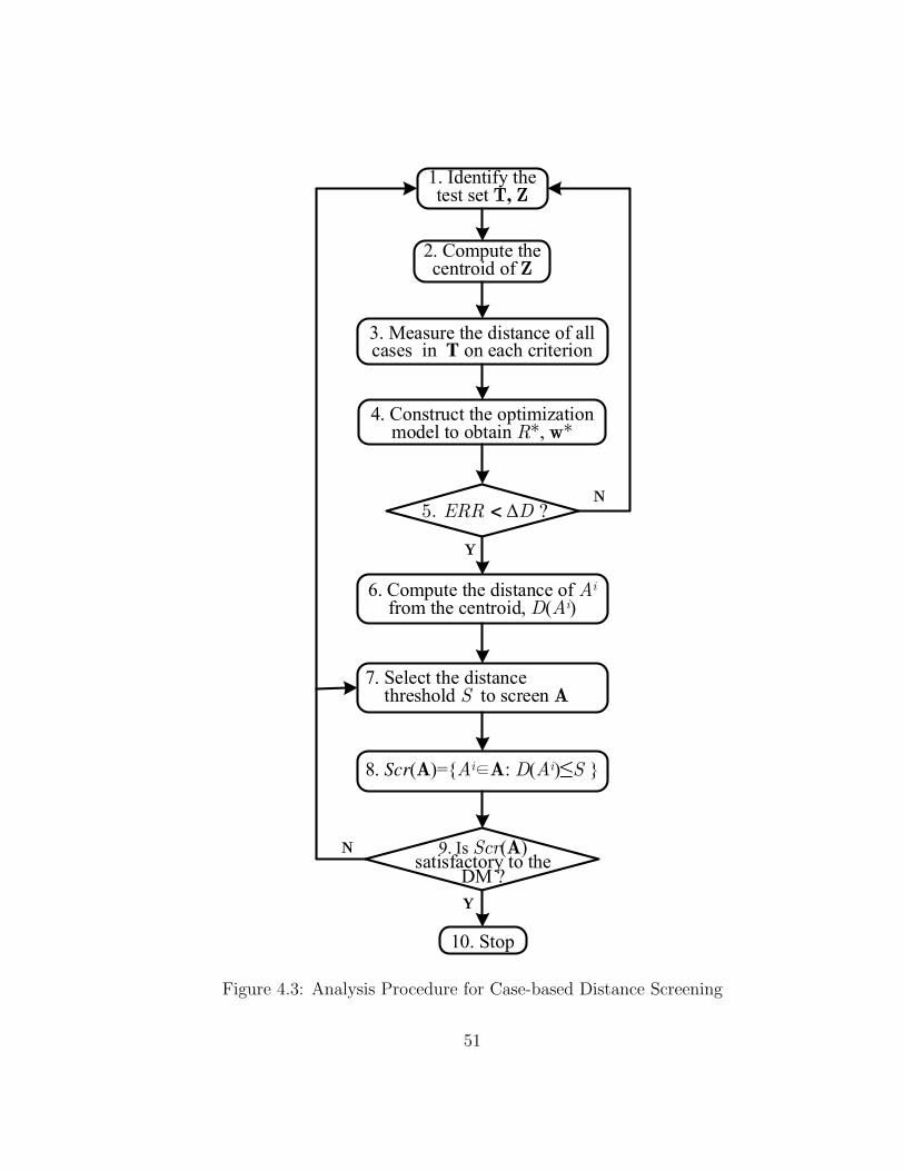
8. Scr(A)={Ai A: D(Ai) S }
1. Identify the test set T, Z
4. Construct the optimization model to obtain R*, w*
6. Compute the distance of Ai
from the centroid, D(Ai)
N
3. Measure the distance of all cases in T on each criterion
9. Is Scr(A)satisfactory to the
DM ?
7. Select the distance threshold S to screen A
Y
10. Stop
5. ERR < D ?
Y
N
2. Compute the centroid of Z
Figure 4.3: Analysis Procedure for Case-based Distance Screening
51
3. Measure the distance of all cases on each criterion: Compute dj(zr, z) for
zr ∈ Z and dj(zp, z) for zp ∈ {T − Z}, using (4.2) and (4.3).
4. Apply the optimization model: The program SCR.2(α) is used to obtain R∗
and w∗.
5. Check the error ERR: When ERR > △D, ask the DM to repeat Step 1; ifERR ≤ △D, go to Step 6.
6. Compute the distance of Ai from the centroid, D(Ai): Based on w∗, obtainthe distance of Ai from the centroid, D(Ai) for Ai ∈ A, using (4.4).
7. Select the distance threshold S: Initially select S = R∗.
8. Screen using S: If D(Ai) is greater than S, then remove Ai; otherwise retainAi. The remaining alternatives are Scr(A).
9. Check the screening result, Scr(A): If Scr(A) is not satisfactory to the DM,either ask the DM to repeat Step 8 for fine tuning, or ask the DM to repeatStep 1 to re-assess the case set, etc.; otherwise stop the screening procedure.For example, when Scr(A) is too large, the DM should first be asked to reduceS in Step 8, alternatively ask the DM to repeat Step 1 to re-assess the caseset.
4.6 Numerical Example
4.6.1 Background
Similar to the WWSP problem described in Chapter 3, it assumed that twelvefeasible alternatives were designed as shown in Table 4.1, and based upon them thebest water resources project need to be identified and implemented for a region.Seven similar criteria, INVEST, OPER, INFRA, ENVIR, RISK, SUPPLY andQUAL, were proposed to evaluate possible alternatives.
4.6.2 Screening Procedure
The test set T = {z1, z2, z3, z4, z5, z6, z7} shown in Table 4.2 is presented to theDM. Assume the DM chooses Z = {z1, z2, z3, z4} as acceptable cases and T− Z =
52
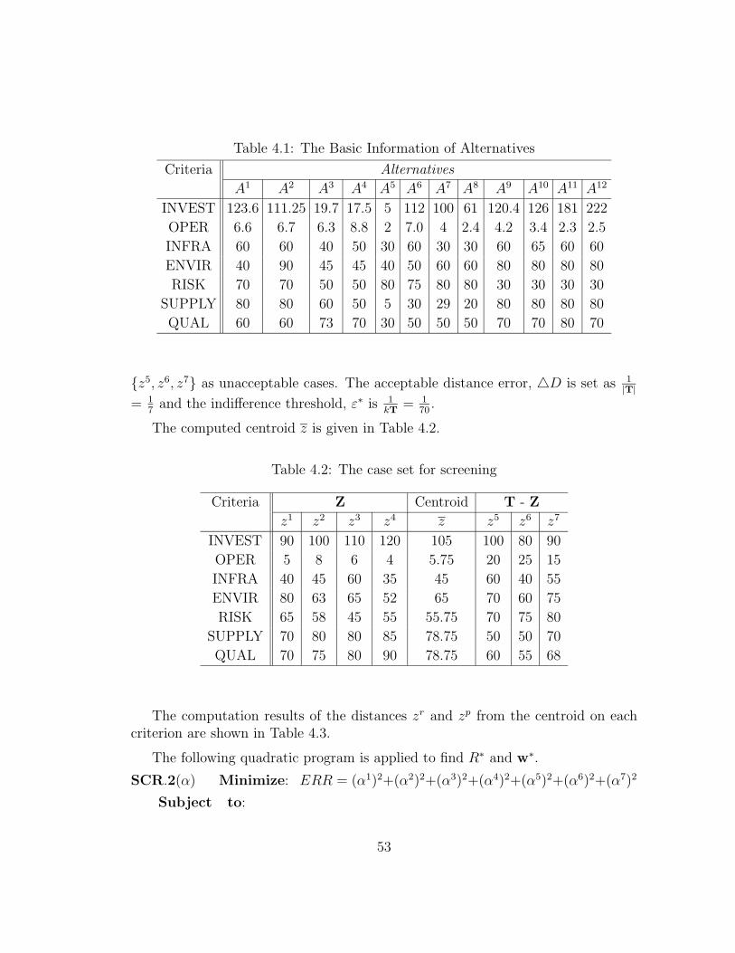
Table 4.1: The Basic Information of Alternatives
Criteria Alternatives
A1 A2 A3 A4 A5 A6 A7 A8 A9 A10 A11 A12
INVEST 123.6 111.25 19.7 17.5 5 112 100 61 120.4 126 181 222
OPER 6.6 6.7 6.3 8.8 2 7.0 4 2.4 4.2 3.4 2.3 2.5
INFRA 60 60 40 50 30 60 30 30 60 65 60 60
ENVIR 40 90 45 45 40 50 60 60 80 80 80 80
RISK 70 70 50 50 80 75 80 80 30 30 30 30
SUPPLY 80 80 60 50 5 30 29 20 80 80 80 80
QUAL 60 60 73 70 30 50 50 50 70 70 80 70
{z5, z6, z7} as unacceptable cases. The acceptable distance error, △D is set as 1|T|
= 17
and the indifference threshold, ε∗ is 1kT
= 170
.
The computed centroid z is given in Table 4.2.
Table 4.2: The case set for screening
Criteria Z Centroid T - Z
z1 z2 z3 z4 z z5 z6 z7
INVEST 90 100 110 120 105 100 80 90
OPER 5 8 6 4 5.75 20 25 15
INFRA 40 45 60 35 45 60 40 55
ENVIR 80 63 65 52 65 70 60 75
RISK 65 58 45 55 55.75 70 75 80
SUPPLY 70 80 80 85 78.75 50 50 70
QUAL 70 75 80 90 78.75 60 55 68
The computation results of the distances zr and zp from the centroid on eachcriterion are shown in Table 4.3.
The following quadratic program is applied to find R∗ and w∗.
SCR.2(α) Minimize: ERR = (α1)2+(α2)2+(α3)2+(α4)2+(α5)2+(α6)2+(α7)2
Subject to:
53
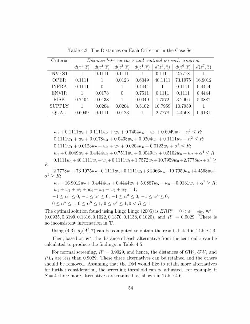
Table 4.3: The Distances on Each Criterion in the Case Set
Criteria Distance between cases and centroid on each criterion
d(z1, z) d(z2, z) d(z3, z) d(z4, z) d(z5, z) d(z6, z) d(z7, z)
INVEST 1 0.1111 0.1111 1 0.1111 2.7778 1
OPER 0.1111 1 0.0123 0.6049 40.1111 73.1975 16.9012
INFRA 0.1111 0 1 0.4444 1 0.1111 0.4444
ENVIR 1 0.0178 0 0.7511 0.1111 0.1111 0.4444
RISK 0.7404 0.0438 1 0.0049 1.7572 3.2066 5.0887
SUPPLY 1 0.0204 0.0204 0.5102 10.7959 10.7959 1
QUAL 0.6049 0.1111 0.0123 1 2.7778 4.4568 0.9131
w1 + 0.1111w2 + 0.1111w3 + w4 + 0.7404w5 + w6 + 0.6049w7 + α1 ≤ R;
0.1111w1 + w2 + 0.0178w4 + 0.0438w5 + 0.0204w6 + 0.1111w7 + α2 ≤ R;
0.1111w1 + 0.0123w2 + w3 + w5 + 0.0204w6 + 0.0123w7 + α3 ≤ R;
w1 + 0.6049w2 + 0.4444w3 + 0.7511w4 + 0.0049w5 + 0.5102w6 + w7 + α4 ≤ R;
0.1111w1+40.1111w2+w3+0.1111w4+1.7572w5+10.7959w6+2.7778w7+α5 ≥R;
2.7778w1+73.1975w2+0.1111w3+0.1111w4+3.2066w5+10.7959w6+4.4568w7+α6 ≥ R;
w1 + 16.9012w2 + 0.4444w3 + 0.4444w4 + 5.0887w5 + w6 + 0.9131w7 + α7 ≥ R;
w1 + w2 + w3 + w4 + w5 + w6 + w7 = 1;
−1 ≤ α1 ≤ 0; −1 ≤ α2 ≤ 0; −1 ≤ α3 ≤ 0; −1 ≤ α4 ≤ 0;
0 ≤ α5 ≤ 1; 0 ≤ α6 ≤ 1; 0 ≤ α7 ≤ 1; 0 < R ≤ 1.
The optimal solution found using Lingo Lingo (2005) is ERR∗ = 0 < ε = 1120
, w∗ =(0.0935, 0.3199, 0.1316, 0.1022, 0.1370, 0.1138, 0.1020), and R∗ = 0.9029. There isno inconsistent information in T.
Using (4.3), dj(Ai, z) can be computed to obtain the results listed in Table 4.4.
Then, based on w∗, the distance of each alternative from the centroid z can becalculated to produce the findings in Table 4.5.
For normal screening, R∗ = 0.9029, and hence, the distances of GW1, GW2 andPL1 are less than 0.9029. These three alternatives can be retained and the othersshould be removed. Assuming that the DM would like to retain more alternativesfor further consideration, the screening threshold can be adjusted. For example, ifS = 4 three more alternatives are retained, as shown in Table 4.6.
54
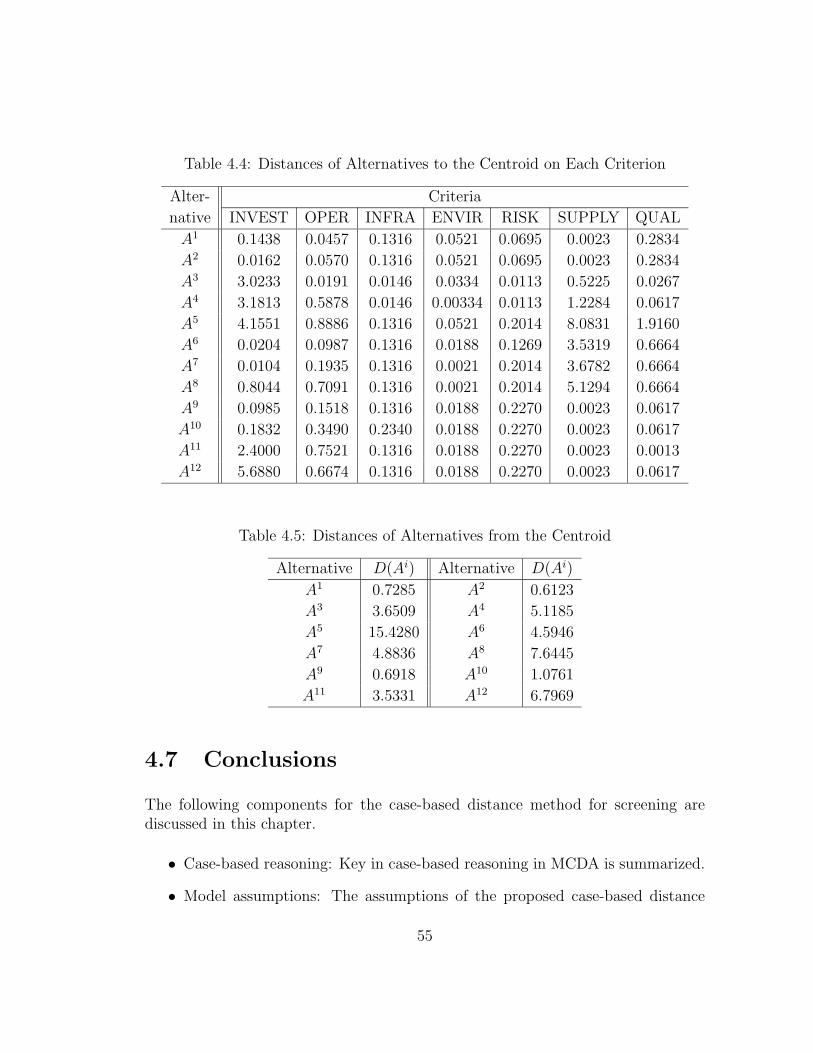
Table 4.4: Distances of Alternatives to the Centroid on Each Criterion
Alter- Criteria
native INVEST OPER INFRA ENVIR RISK SUPPLY QUAL
A1 0.1438 0.0457 0.1316 0.0521 0.0695 0.0023 0.2834
A2 0.0162 0.0570 0.1316 0.0521 0.0695 0.0023 0.2834
A3 3.0233 0.0191 0.0146 0.0334 0.0113 0.5225 0.0267
A4 3.1813 0.5878 0.0146 0.00334 0.0113 1.2284 0.0617
A5 4.1551 0.8886 0.1316 0.0521 0.2014 8.0831 1.9160
A6 0.0204 0.0987 0.1316 0.0188 0.1269 3.5319 0.6664
A7 0.0104 0.1935 0.1316 0.0021 0.2014 3.6782 0.6664
A8 0.8044 0.7091 0.1316 0.0021 0.2014 5.1294 0.6664
A9 0.0985 0.1518 0.1316 0.0188 0.2270 0.0023 0.0617
A10 0.1832 0.3490 0.2340 0.0188 0.2270 0.0023 0.0617
A11 2.4000 0.7521 0.1316 0.0188 0.2270 0.0023 0.0013
A12 5.6880 0.6674 0.1316 0.0188 0.2270 0.0023 0.0617
Table 4.5: Distances of Alternatives from the Centroid
Alternative D(Ai) Alternative D(Ai)
A1 0.7285 A2 0.6123
A3 3.6509 A4 5.1185
A5 15.4280 A6 4.5946
A7 4.8836 A8 7.6445
A9 0.6918 A10 1.0761
A11 3.5331 A12 6.7969
4.7 Conclusions
The following components for the case-based distance method for screening arediscussed in this chapter.
• Case-based reasoning: Key in case-based reasoning in MCDA is summarized.
• Model assumptions: The assumptions of the proposed case-based distance
55
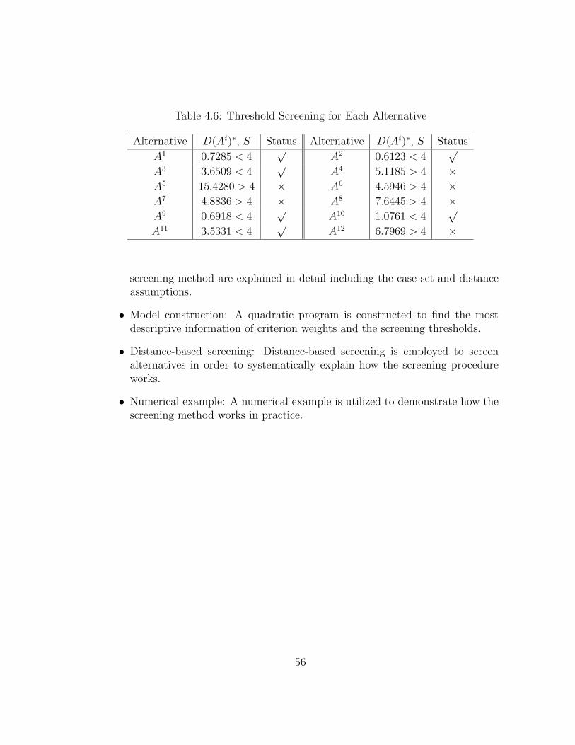
Table 4.6: Threshold Screening for Each Alternative
Alternative D(Ai)∗, S Status Alternative D(Ai)∗, S Status
A1 0.7285 < 4√
A2 0.6123 < 4√
A3 3.6509 < 4√
A4 5.1185 > 4 ×A5 15.4280 > 4 × A6 4.5946 > 4 ×A7 4.8836 > 4 × A8 7.6445 > 4 ×A9 0.6918 < 4
√A10 1.0761 < 4
√
A11 3.5331 < 4√
A12 6.7969 > 4 ×
screening method are explained in detail including the case set and distanceassumptions.
• Model construction: A quadratic program is constructed to find the mostdescriptive information of criterion weights and the screening thresholds.
• Distance-based screening: Distance-based screening is employed to screenalternatives in order to systematically explain how the screening procedureworks.
• Numerical example: A numerical example is utilized to demonstrate how thescreening method works in practice.
56
Chapter 5
Sorting Problems in MultipleCriteria Decision Analysis
5.1 Introduction
The case-based distance screening method is extended to solve sorting problems inMCDA, in order to arrange a set of alternatives into a few predefined groups inpreference order so that the DM can manage them more efficiently and effectively.Firstly, a general description of sorting problems is presented in detail including aformal definition of a sorting procedure and a discussion of relationship between thealternative set and the sorting group set. Based on weighted Euclidean distance,two case-based distance models are developed for sorting using weights and groupthresholds obtained by the assessment of a case set provided by a decision maker.Case-based sorting model I is designed for cardinal criteria; its extension, case-based sorting model II, can handle both cardinal and ordinal criteria. Optimizationprograms are employed to find the most descriptive weights and group thresholds.Finally, a case study on analyzing Canadian municipal water usage is presented.Earlier versions of the research contained in this chapter are provided by Chen etal. (2005a); Chen et al. (2005d).
5.2 General Description of Sorting Problems
A formal definition of a sorting procedure in MCDA is as follows:
57
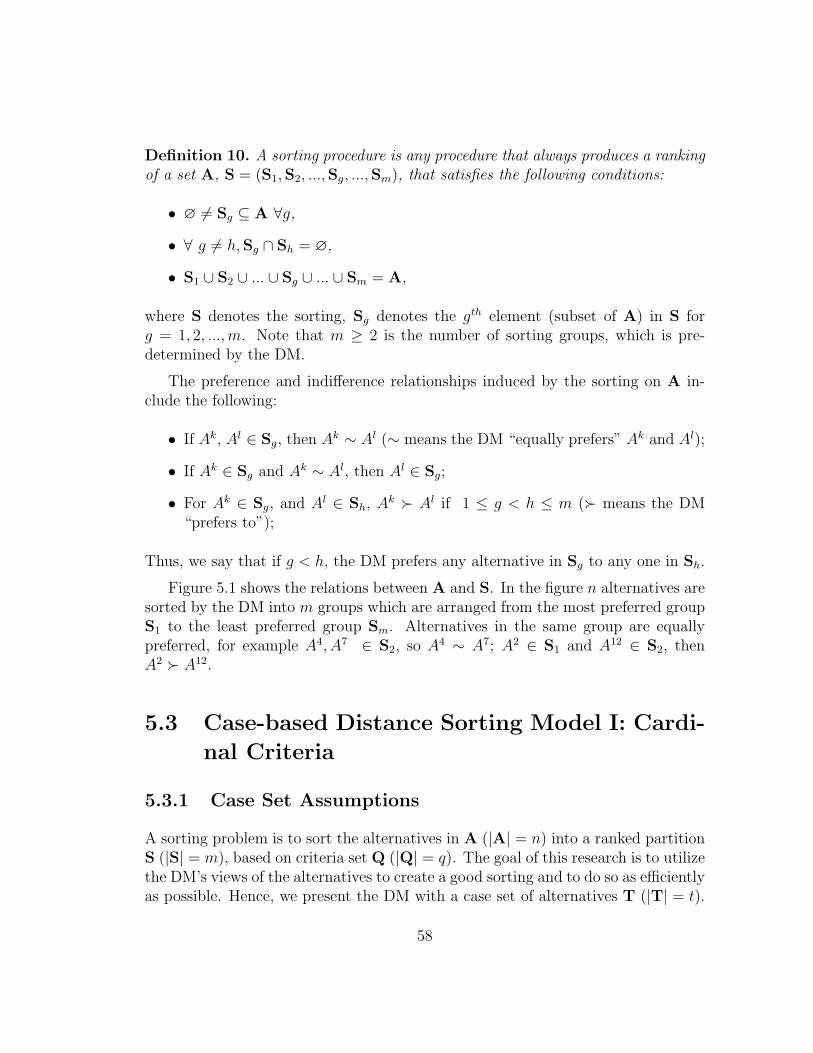
Definition 10. A sorting procedure is any procedure that always produces a rankingof a set A, S = (S1,S2, ...,Sg, ...,Sm), that satisfies the following conditions:
• ∅ 6= Sg ⊆ A ∀g,
• ∀ g 6= h,Sg ∩ Sh = ∅,
• S1 ∪ S2 ∪ ... ∪ Sg ∪ ... ∪ Sm = A,
where S denotes the sorting, Sg denotes the gth element (subset of A) in S forg = 1, 2, ...,m. Note that m ≥ 2 is the number of sorting groups, which is pre-determined by the DM.
The preference and indifference relationships induced by the sorting on A in-clude the following:
• If Ak, Al ∈ Sg, then Ak ∼ Al (∼ means the DM “equally prefers” Ak and Al);
• If Ak ∈ Sg and Ak ∼ Al, then Al ∈ Sg;
• For Ak ∈ Sg, and Al ∈ Sh, Ak ≻ Al if 1 ≤ g < h ≤ m (≻ means the DM“prefers to”);
Thus, we say that if g < h, the DM prefers any alternative in Sg to any one in Sh.
Figure 5.1 shows the relations between A and S. In the figure n alternatives aresorted by the DM into m groups which are arranged from the most preferred groupS1 to the least preferred group Sm. Alternatives in the same group are equallypreferred, for example A4, A7 ∈ S2, so A4 ∼ A7; A2 ∈ S1 and A12 ∈ S2, thenA2 ≻ A12.
5.3 Case-based Distance Sorting Model I: Cardi-
nal Criteria
5.3.1 Case Set Assumptions
A sorting problem is to sort the alternatives in A (|A| = n) into a ranked partitionS (|S| = m), based on criteria set Q (|Q| = q). The goal of this research is to utilizethe DM’s views of the alternatives to create a good sorting and to do so as efficientlyas possible. Hence, we present the DM with a case set of alternatives T (|T| = t).
58
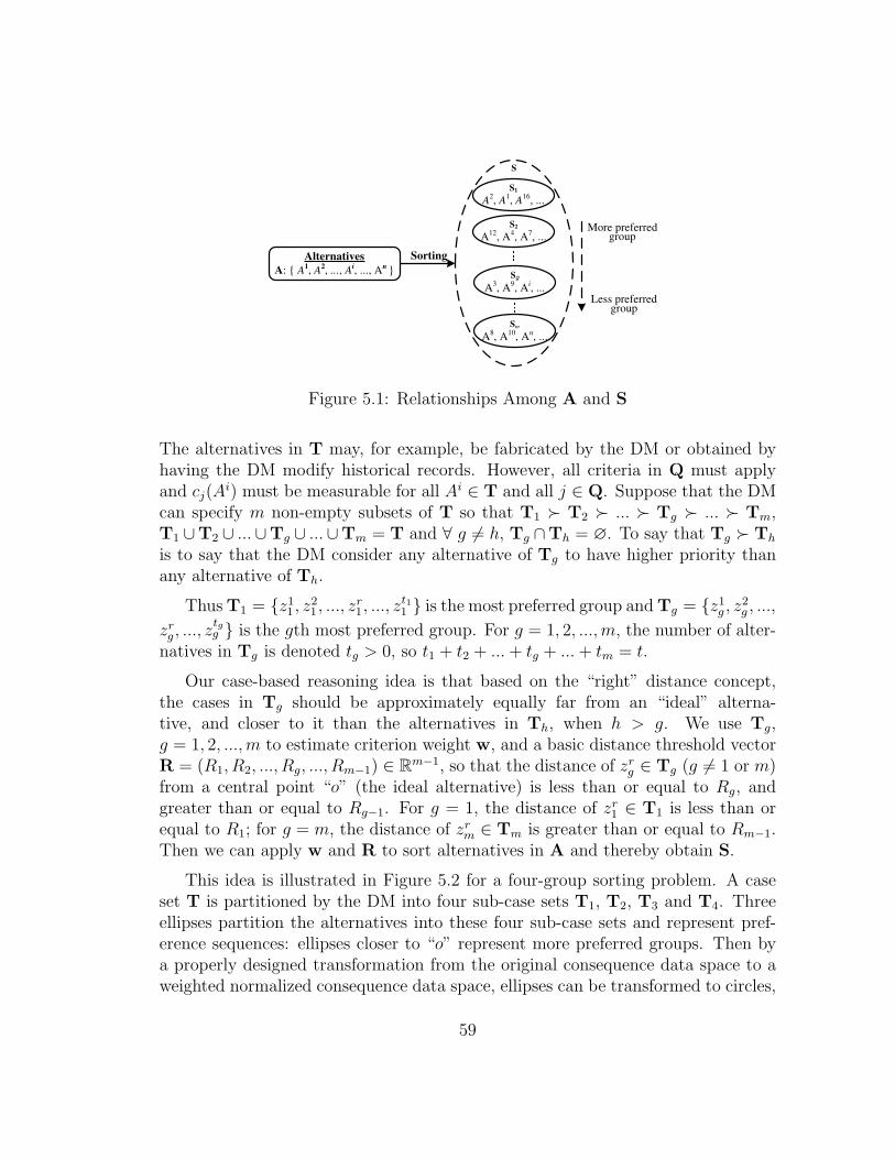
Alternatives
A: { A1, A2, ..., A
i, ..., An }
More preferred group
Less preferred group
Sorting
S1
A2, A
1, A
16, ...
S2
A12
, A4, A
7, ...
Sg
A3, A
9, A
i, ...
Sm
A8, A10, An, ...
S
Figure 5.1: Relationships Among A and S
The alternatives in T may, for example, be fabricated by the DM or obtained byhaving the DM modify historical records. However, all criteria in Q must applyand cj(A
i) must be measurable for all Ai ∈ T and all j ∈ Q. Suppose that the DMcan specify m non-empty subsets of T so that T1 ≻ T2 ≻ ... ≻ Tg ≻ ... ≻ Tm,T1 ∪T2 ∪ ...∪Tg ∪ ...∪Tm = T and ∀ g 6= h, Tg ∩Th = ∅. To say that Tg ≻ Th
is to say that the DM consider any alternative of Tg to have higher priority thanany alternative of Th.
Thus T1 = {z11 , z
21 , ..., z
r1, ..., z
t11 } is the most preferred group and Tg = {z1
g , z2g , ...,
zrg , ..., z
tgg } is the gth most preferred group. For g = 1, 2, ...,m, the number of alter-
natives in Tg is denoted tg > 0, so t1 + t2 + ... + tg + ... + tm = t.
Our case-based reasoning idea is that based on the “right” distance concept,the cases in Tg should be approximately equally far from an “ideal” alterna-tive, and closer to it than the alternatives in Th, when h > g. We use Tg,g = 1, 2, ...,m to estimate criterion weight w, and a basic distance threshold vectorR = (R1, R2, ..., Rg, ..., Rm−1) ∈ Rm−1, so that the distance of zr
g ∈ Tg (g 6= 1 or m)from a central point “o” (the ideal alternative) is less than or equal to Rg, andgreater than or equal to Rg−1. For g = 1, the distance of zr
1 ∈ T1 is less than orequal to R1; for g = m, the distance of zr
m ∈ Tm is greater than or equal to Rm−1.Then we can apply w and R to sort alternatives in A and thereby obtain S.
This idea is illustrated in Figure 5.2 for a four-group sorting problem. A caseset T is partitioned by the DM into four sub-case sets T1, T2, T3 and T4. Threeellipses partition the alternatives into these four sub-case sets and represent pref-erence sequences: ellipses closer to “o” represent more preferred groups. Then bya properly designed transformation from the original consequence data space to aweighted normalized consequence data space, ellipses can be transformed to circles,
59
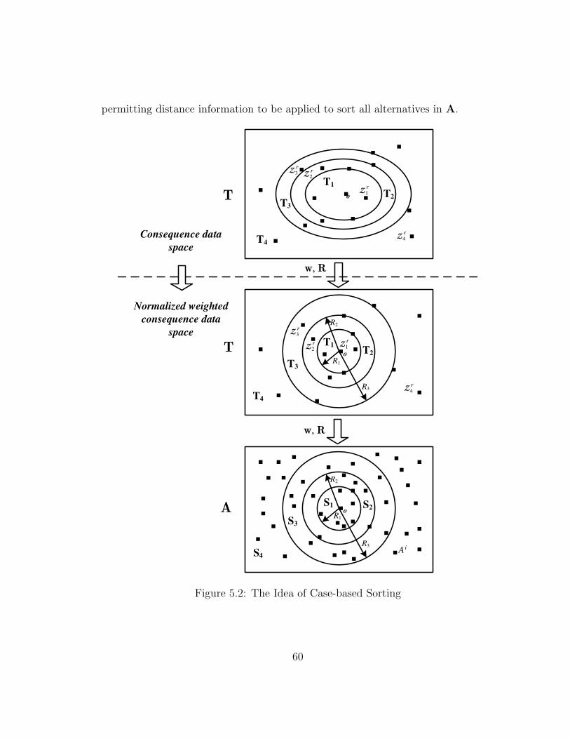
permitting distance information to be applied to sort all alternatives in A.
Normalized weighted
consequence data
space
w, R
.
.
.
T1
T
.
.
.
.
.
z r1
.
T2
T3
.z r2
z r3
.
.
.
z r4T4
T
o.
o.T1
.
.
.
.
R1
T2
.
.
.
z r1z r
2
R2
T3
.
.
.
.
z r3
R3
.
..
.
z r4
T4
w, R
A o.S1
.
.
.
.
.
.
R1
S2
.
.
.
.
.
.
R2
S3
.
.
.
.
.
.
.
.
R3
.
.
.
.
.
.
..
.
.
S4A i
.
.
.
.
.
..
.
.
.
.
.
.
.
.
.
.
Consequence data
space
Figure 5.2: The Idea of Case-based Sorting
60
5.3.2 Distance Assumptions
Given the most preferred alternatives in the case set T1, the centroid of T1, z+, ischosen to be the fictitious “ideal” alternative, at the center of T1. By definition,
cj(z+) =1
t1
t1∑
r=1
cj(zr1). (5.1)
Similarly, for the case set Tm, a fictitious alternative, z−, the centroid of Tm, isdeemed to be a fictitious alternative at the center of Tm.
cj(z−) =1
tm
tm∑
r=1
cj(zrm). (5.2)
Note that an “ideal” point can also be based on T2, T3, ..., Tm−1, but we use onlythe two extremes.
For j = 1, 2, ..., q, define dmax +j =
mmaxg=1
tgmaxr=1
(
cj(zrg) − cj(z+)
)2to be the normal-
ization factor for criterion j. For g = 1, 2, ..,m and r = 1, 2, ..., tg, the distancebetween zr
g ∈ Tg and the centroid z+ on criterion j is
dj(zrg , z+) =
(
cj(zrg) − cj(z+)
)2
dmax +j
. (5.3)
Similarly, the distance between alternative Ai ∈ A and the centroid z+ on criterionj is
dj(Ai, z+) =
(
cij − cj(z+)
)2
dmax +j
. (5.4)
Note that 0 ≤ dj(zrg , z+) ≤ 1. Also 0 < dj(A
i, z+), but dj(Ai, z+) could be larger
than 1.
Weighted Euclidean distance is employed since it has a clear geometric meaning,which can be easily understood and accepted by the DM to represent his or heraggregated preference. The relative order of non-negative numbers (distances) isthe same as the relative order of their squares. For this reason, instead of Euclideandistances we use their squares, because they are easier to compute while preservingorder. The aggregated distance between alternatives zr
g ∈ Tg and z+ over thecriteria set Q is identified as
D(zrg)+ = D(zr
g , z+) =∑
j∈Q
wj · dj(zrg , z+),
61
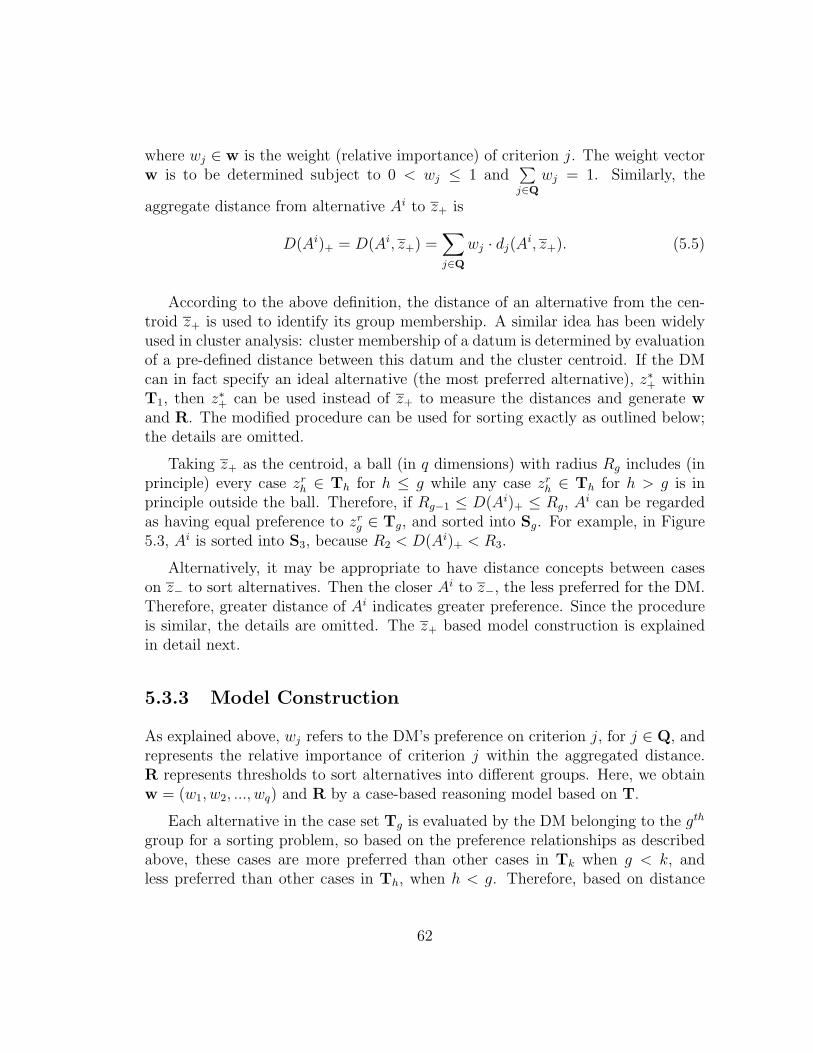
where wj ∈ w is the weight (relative importance) of criterion j. The weight vectorw is to be determined subject to 0 < wj ≤ 1 and
∑
j∈Q
wj = 1. Similarly, the
aggregate distance from alternative Ai to z+ is
D(Ai)+ = D(Ai, z+) =∑
j∈Q
wj · dj(Ai, z+). (5.5)
According to the above definition, the distance of an alternative from the cen-troid z+ is used to identify its group membership. A similar idea has been widelyused in cluster analysis: cluster membership of a datum is determined by evaluationof a pre-defined distance between this datum and the cluster centroid. If the DMcan in fact specify an ideal alternative (the most preferred alternative), z∗+ withinT1, then z∗+ can be used instead of z+ to measure the distances and generate wand R. The modified procedure can be used for sorting exactly as outlined below;the details are omitted.
Taking z+ as the centroid, a ball (in q dimensions) with radius Rg includes (inprinciple) every case zr
h ∈ Th for h ≤ g while any case zrh ∈ Th for h > g is in
principle outside the ball. Therefore, if Rg−1 ≤ D(Ai)+ ≤ Rg, Ai can be regardedas having equal preference to zr
g ∈ Tg, and sorted into Sg. For example, in Figure5.3, Ai is sorted into S3, because R2 < D(Ai)+ < R3.
Alternatively, it may be appropriate to have distance concepts between caseson z− to sort alternatives. Then the closer Ai to z−, the less preferred for the DM.Therefore, greater distance of Ai indicates greater preference. Since the procedureis similar, the details are omitted. The z+ based model construction is explainedin detail next.
5.3.3 Model Construction
As explained above, wj refers to the DM’s preference on criterion j, for j ∈ Q, andrepresents the relative importance of criterion j within the aggregated distance.R represents thresholds to sort alternatives into different groups. Here, we obtainw = (w1, w2, ..., wq) and R by a case-based reasoning model based on T.
Each alternative in the case set Tg is evaluated by the DM belonging to the gth
group for a sorting problem, so based on the preference relationships as describedabove, these cases are more preferred than other cases in Tk when g < k, andless preferred than other cases in Th, when h < g. Therefore, based on distance
62
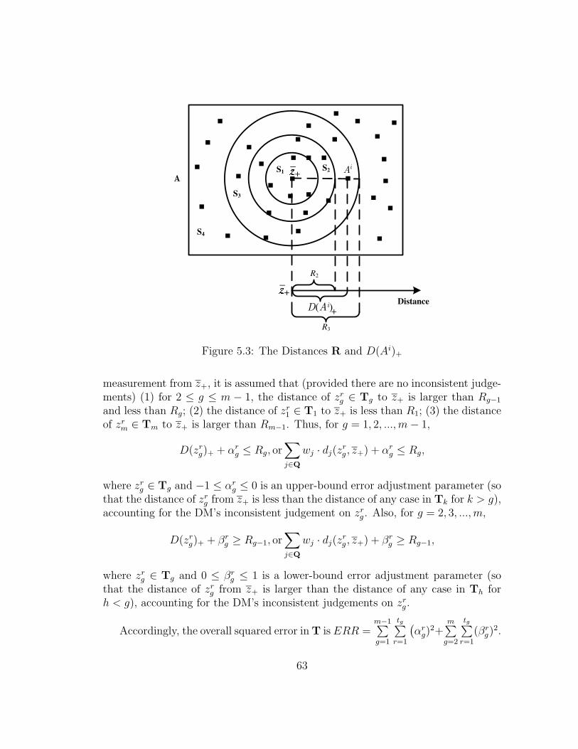
A .
S1
.
.
.
.
.
S2
.
..
.
.
.
S3
.
.
..
.
.
.
.
.
.
.
.
.
.
.
.
.
.
.
.
S4
_+
R2
_+
R3
Distance
.
Ai
D(Ai)+
Figure 5.3: The Distances R and D(Ai)+
measurement from z+, it is assumed that (provided there are no inconsistent judge-ments) (1) for 2 ≤ g ≤ m − 1, the distance of zr
g ∈ Tg to z+ is larger than Rg−1
and less than Rg; (2) the distance of zr1 ∈ T1 to z+ is less than R1; (3) the distance
of zrm ∈ Tm to z+ is larger than Rm−1. Thus, for g = 1, 2, ...,m − 1,
D(zrg)+ + αr
g ≤ Rg, or∑
j∈Q
wj · dj(zrg , z+) + αr
g ≤ Rg,
where zrg ∈ Tg and −1 ≤ αr
g ≤ 0 is an upper-bound error adjustment parameter (sothat the distance of zr
g from z+ is less than the distance of any case in Tk for k > g),accounting for the DM’s inconsistent judgement on zr
g . Also, for g = 2, 3, ...,m,
D(zrg)+ + βr
g ≥ Rg−1, or∑
j∈Q
wj · dj(zrg , z+) + βr
g ≥ Rg−1,
where zrg ∈ Tg and 0 ≤ βr
g ≤ 1 is a lower-bound error adjustment parameter (sothat the distance of zr
g from z+ is larger than the distance of any case in Th forh < g), accounting for the DM’s inconsistent judgements on zr
g .
Accordingly, the overall squared error in T is ERR =m−1∑
g=1
tg∑
r=1
(
αrg)
2+m∑
g=2
tg∑
r=1
(βrg)
2.
63
Based on z+, the following optimization model can be used to find the most de-scriptive weight vector w and the distance threshold vector R.
SOR.1(α, β) Minimize : ERR =m−1∑
g=1
tg∑
r=1
(
αrg)
2 +m∑
g=2
tg∑
r=1
(βrg)
2
Subject to:∑
j∈Q
wj · dj(zrg , z+) + αr
g ≤ Rg,
r = 1, 2, ..., tg, g = 1, 2, ...,m − 1;∑
j∈Q
wj · dj(zrg , z+) + βr
g ≥ Rg−1,
r = 1, 2, ..., tg, g = 2, 3, ...,m;
Rg−1 < Rg, g = 2, ...,m − 1;
−1 ≤ αrg ≤ 0, g = 1, ...,m − 1;
0 ≤ βrg ≤ 1, g = 2, ...,m;
wj > 0;∑
j∈Q
wj = 1.
The optimal solutions of SOR.1(α, β) are denoted by w∗ and R∗, respectively, andERR∗ is the minimal value of ERR.
Theorem 5. SOR.1(α, β) has at least one optimal solution.
Proof: The constraints in SOR.1(α, β) constitute a convex set. The objec-
tive function ERR =m−1∑
g=1
tg∑
r=1
(
αrg)
2 +m∑
g=2
tg∑
r=1
(βrg)
2 is a quadratic function on this
set. Based on the extreme value theorem of advanced calculus (Fitzpatrick, 1995,page 297), the function ERR is continuous and the set of all possible variables isbounded, ERR attains its minimum at least once. ¤
Two threshold parameters can be set by the DM to evaluate the errors generatedby SOR.1(α, β) as follows:
(1) The acceptable distance error, ∆D: ∆D is the threshold below which the errorgenerated by SOR.1(α, β) is acceptable to the DM. If ERR∗ ≤ ∆D, the errorsare acceptable; otherwise T should be reset. A suggested value of ∆D is 1
10t,
where t = |T|.
64
(2) The indifference threshold (see Vincke (1992) for detailed discussion of indiffer-ence threshold in MCDA) ε: ε is the threshold below which errors generated bySOR.1(α, β) can be ignored. When ERR∗ ≤ ε, the case set T holds consistentinformation; when ERR∗ ≥ ε, the errors cannot be ignored and there is someinconsistency in T. A suggested value of ε is 1
10n, where n = |A|. Usually 1
10nis
small enough to affect (but not strongly) the balance between the indifferencethreshold and acceptable error. Of course, in practice the DM should increaseor decrease ε as desired.
5.3.4 Distance-based Sorting
Assuming ERR∗ ≤ ∆D, with w∗ = (w∗1, w
∗2, ..., w
∗q) obtained from SOR.1(α, β),
the maximum upper-bound error in Tg is denoted as αmaxg = max
r=1,2,...,tg{|αr
g|} and the
maximum lower-bound error in Tg is denoted as βmaxg = max
r=1,2,...,tg{βr
g}. Different
policies to set the sorting distance thresholds based on R can be employed to carryout sorting.
(1) Normal Sorting : When ERR∗ ≤ ε, the errors can be ignored and R∗ =(R∗
1, R∗2, ..., R
∗g, ..., R
∗m−1) is utilized to sort alternatives.
• If D(Ai)+ ≤ R∗1, Ai ∈ S1;
• If R∗1 < D(Ai)+ ≤ R∗
2, Ai ∈ S2;
· · · · · ·• If R∗
g−1 < D(Ai)+ ≤ R∗g, Ai ∈ Sg;
· · · · · ·• If D(Ai)+ > R∗
m−1, Ai ∈ Sm.
(2) Conservative Sorting: For ERR∗ ≥ ε, αmaxg is taken into account as error
permission in T. The distance thresholds are defined as (R∗1 + αmax
1 , R∗2 +
αmax2 , ..., R∗
g + αmaxg , ..., R∗
m−1 + αmaxm−1) and used to sort alternatives.
• If D(Ai)+ ≤ R∗1 + αmax
1 , Ai ∈ S1;
• If R∗1 + αmax
1 < D(Ai)+ ≤ R∗2 + αmax
2 , Ai ∈ S2;
· · · · · ·• If R∗
g−1 + αmaxg−1 < D(Ai)+ ≤ R∗
g + αmaxm , Ai ∈ Sg;
· · · · · ·
65
• If D(Ai)+ > R∗m−1 + αmax
m−1, Ai ∈ Sm.
(3) Aggressive Sorting: For ERR∗ ≥ ε, βmaxg is taken into account as error
reduction in T. The distance thresholds are defined as (R∗1 − βmax
1 , R∗2 −
βmax2 , ..., R∗
g − βmaxg , ..., R∗
m−1 − βmaxm−1) and employed to sort alternatives (We
assume R∗g − βmax
g > 0 for g = 1, 2, ...,m).
• If D(Ai)+ ≤ R∗1 − βmax
1 , Ai ∈ S1;
• If R∗1 − βmax
1 < D(Ai)+ ≤ R∗2 − βmax
2 , Ai ∈ S2;
· · · · · ·• If R∗
g−1 − βmaxg−1 < D(Ai)+ ≤ R∗
g − βmaxm , Ai ∈ Sg;
· · · · · ·• If D(Ai)+ > R∗
m−1 − βmaxm−1, Ai ∈ Sm.
Note that based on the setting of the acceptable distance error, △D, αmaxg and
βmaxg are much smaller than any distance threshold, R∗
g. Hence, there is no reversingthe ordering of classes.
5.3.5 Sorting Consistency
Based on the z+ sorting method, the procedures explained above can be im-plemented to obtain w∗ and R∗ and accordingly to generate a sorting S+ =(S+
1 ,S+2 , ...,S+
g , ...,S+m) for A. Similar procedures can be carried out based on the z−
sorting method to obtain another sorting for A denoted as S− = (S−1 ,S−
2 , ...,S−g , ...,
S−m). The following method is proposed to compare the z+ and z− sortings and
provide the DM with more information to evaluate the sorting results.
The proportion of alternatives in S+g to alternatives in A is ρ+
g = 1n|S+
g | for g =1, 2, ...,m, where n is the number of alternatives in A and . Similarly, ρ−
g = 1n|S−
g |is the proportion of alternatives in S−
g to alternatives in A.
Let Φ+ represent the vector constituting of ρ+1 , ρ+
2 , ..., ρ+m, sorted into decreasing
order and similarly for Φ−. When Φ+ = Φ−, we say that the case set T gives aroughly consistent sorting beginning with both the most preferred group T1
and the least preferred group Tm. Let Cg denote the core alternatives for sortinggroup g, such that Cg = {S+
g ∩ S−g } for g = 1, 2, ...,m. The degree of consistency
for T is defined as ρT = 1n
∑mg=1 |Cg|.
66
5.4 Case-based Sorting Model II: Ordinal and
Cardinal Criteria
5.4.1 Ordinal Criteria in MCDA
MCDA problems may involve the evaluation of ordinal criteria, such as customersatisfaction or priority. Consequence data cannot be naturally connected to ordinalcriteria. Many researchers have studied how to handle ordinal criteria in MCDA,and some approaches are summarized next.
Many methods have been proposed to acquire directly a reasonable value datum(vi
j) without measurement and transformation from a consequence (cij). In the
context of linear additive value (utility) functions, as in (2.5), Sage and White(1984) propose an imprecisely specified multiattribute utility theory (ISMAUT)model to handle ordinal criteria. Malakooti (2000) suggests a method to rank andscreen alternatives based on partial preference information. Ahn (2003) extendsMalakooti’s work to include preference strength and partial information.
Several fuzzy set theory methods have been proposed to handle ordinal criteria,for example, Chen (1996); Herrera-Viedma et al. (2002). Most of them share asimilar idea; instead of directly expressing preferences on ordinal criteria for eachalternative, the DM asks experts to evaluate alternatives on each criterion usinga pre-defined linguistic grade set, such as poor, neutral, good, very good. Thenthe DM assigns these ordinal statements fuzzy membership functions and employsaggregation models to obtain final conclusions. Similarly, based on the Dempster- Shafer theory of evidence, Yang and Xu (2002) develop an evidential reasoningapproach to handle qualitative (ordinal) criteria.
Instead of the methods described above, which may involve complicated math-ematical computations, one simple but efficient approach to deal with ordinal cri-teria is to ask a DM to consider whether there is cardinal information connectedto ordinal criteria in an MCDA problem. By careful thinking, the DM may findproxy cardinal criteria representing ordinal criteria, permitting ordinal criteria tobe transformed to relevant cardinal criteria. The advantages of such methods arethat the DM’s objectives for a decision problem are clarified and the DM mayfeel more confident of the final conclusions. Keeney (1992) proposes a systematicanalysis method, value-focused thinking, which is an analytic approach to identifyand define criteria properly. For example, Keeney recounts how it is difficult tofind a direct criterion to represent the damage to historic buildings from acid rain,but a useful proxy criterion could be sulphur dioxide concentration in rain water.
67
Another application of value-focused thinking in cell phone plan design is given inKeeney (2004).
5.4.2 Ordinal Criteria Expressions
Sometimes the DM may not easily find suitable proxy cardinal criteria representingordinal criteria for an MCDA problem. The following method is developed toincorporate ordinal criteria into our proposed case-based distance sorting model.
Recall that Q is the set of criteria. When ordinal criteria are involved, assumethat Q can be partitioned into QCRD and QORD, which represent the cardinal andordinal criteria sets, respectively. Obviously, Q = QCRD ∪ QORD, and QCRD ∩QORD = ∅.
For each ordinal criterion j ∈ QORD, we arrange a linguistic grade set, suchas very good, good, fair, neutral, poor to directly evaluate the alternatives. Thelinguistic grade set is L = (1, 2, ..., l, ..., L), where 1 is the best linguistic evaluationand L is the worst. Then a value interval, vi
j, can be assigned to Ai to representits linguistic evaluation on each ordinal criterion. For example, with the z+ sortingmethod, Ai ∈ A, if Ai is evaluated belonging to the best grade, then vi
j ∈ [0, 1L]. The
detailed relationships between linguistic evaluation grade and value interval for thez+ sorting method are listed in Table 5.1. For z− sorting method, linguistic evalua-tion grade and value interval have the opposite relationship. Note that without lossof generality, we assume vi
j ∈ [ liL, li+1
L]. When vi
j is applied to T, vj(zrg) ∈ [ lr
L, lr+1
L]
is used to represent the value interval of zrg on the ordinal criterion j ∈ QORD.
Table 5.1: Linguistic Evaluation Grade and Value Interval for z+ Sorting Method
linguistic evaluations Value intervals
1 [0, 1L]
2 [ 1L, 2
L]
3 [ 2L, 3
L]
· · · [· · · , · · · ]l [ l
L, l+1
L]
· · · [· · · , · · · ]L [L−1
L, 1]
68
5.4.3 Case-based Sorting Model Incorporating Ordinal Cri-teria
Assuming Q = QCRD ∪ QORD, with the z+ sorting method, the cardinal criteriaset, QCRD part of z+ can be calculated using (5.1). For the ordinal criteria set,QORD, there is no consequence centroid, but the best linguistic grade can be re-garded as an ideal point and used to measure the distance. Therefore, we assigndj(z
rg , z+) = (vj(z
rg))
2 for j ∈ QORD. For QCRD, Equation (4.3) is still applicable toobtain dj(z
rg , z+). The aggregated distance of zr
g under both cardinal and ordinalcriteria is defined as
D(zrg)+ =
∑
j∈QCRD
wj · dj(zrg , z+) +
∑
j∈QORD
wj · (vj(zrg))
2. (5.6)
Note that (5.6) can be applied to A.
Similarly, the following optimization model can be used to find the most descrip-tive weight vector w and the distance threshold vector R for z+ sorting incorporatedordinal criteria.
SOR.2(α, β) Minimize : ERR =m−1∑
g=1
tg∑
r=1
(
αrg)
2 +m∑
g=2
tg∑
r=1
(βrg)
2
Subject to:∑
j∈QCRD
wj · dj(zrg , z+) +
∑
j∈QORD
wj · (vj(zrg))
2 + αrg ≤ Rg,
r = 1, 2, ..., tg, g = 1, 2, ...,m − 1;∑
j∈QCRD
wj · dj(zrg , z+) +
∑
j∈QORD
wj · (vj(zrg))
2 + βrg ≥ Rg−1,
r = 1, 2, ..., tg, g = 2, 3, ...,m;
Rg−1 < Rg, g = 2, ...,m − 1;
−1 ≤ αrg ≤ 0, g = 1, ...,m − 1;
0 ≤ βrg ≤ 1, g = 2, ...,m;
wj > 0; wj > 0;∑
j∈QCRD
wj +∑
j∈QORD
wj = 1;
vj(zrg) ∈ [ lr
L, lr+1
L], r = 1, 2, ..., tg, g = 1, 2, 3, ...,m.
Similarly SOR.2(α, β) generates at least one optimal solution w∗ and R∗. Thesuggested value of the indifference threshold, ε, and the acceptable distance error,∆D remain the same as the ones described in Section 5.3.
69
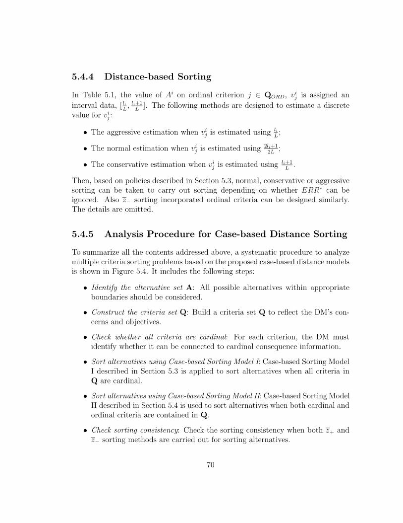
5.4.4 Distance-based Sorting
In Table 5.1, the value of Ai on ordinal criterion j ∈ QORD, vij is assigned an
interval data, [ liL, li+1
L]. The following methods are designed to estimate a discrete
value for vij:
• The aggressive estimation when vij is estimated using li
L;
• The normal estimation when vij is estimated using 2li+1
2L;
• The conservative estimation when vij is estimated using li+1
L.
Then, based on policies described in Section 5.3, normal, conservative or aggressivesorting can be taken to carry out sorting depending on whether ERR∗ can beignored. Also z− sorting incorporated ordinal criteria can be designed similarly.The details are omitted.
5.4.5 Analysis Procedure for Case-based Distance Sorting
To summarize all the contents addressed above, a systematic procedure to analyzemultiple criteria sorting problems based on the proposed case-based distance modelsis shown in Figure 5.4. It includes the following steps:
• Identify the alternative set A: All possible alternatives within appropriateboundaries should be considered.
• Construct the criteria set Q: Build a criteria set Q to reflect the DM’s con-cerns and objectives.
• Check whether all criteria are cardinal: For each criterion, the DM mustidentify whether it can be connected to cardinal consequence information.
• Sort alternatives using Case-based Sorting Model I: Case-based Sorting ModelI described in Section 5.3 is applied to sort alternatives when all criteria inQ are cardinal.
• Sort alternatives using Case-based Sorting Model II: Case-based Sorting ModelII described in Section 5.4 is used to sort alternatives when both cardinal andordinal criteria are contained in Q.
• Check sorting consistency: Check the sorting consistency when both z+ andz− sorting methods are carried out for sorting alternatives.
70
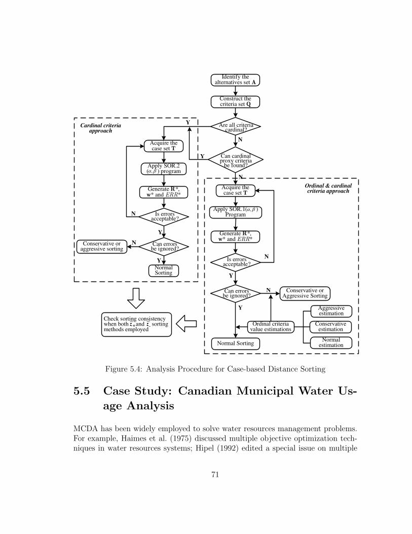
Identify the alternatives set A
Y
Construct the criteria set Q
Generate R*,w* and ERR*
Is errors acceptable?
Acquire the case set T
N
Normal Sorting
Y
Can errors be ignored?
Y
Conservative or aggressive sorting
N
N
Y Can cardinal proxy criteria
be found?
N
Acquire the case set T
Generate R*,w* and ERR*
Is errors acceptable?
Y
Can errors be ignored?
Normal Sorting
Y
Ordinal criteria value estimations
Conservative or Aggressive Sorting
N
N
Cardinal criteria approach
Aggressive estimation
Conservative estimation
Normal estimation
Ordinal & cardinal criteria approach
Apply SOR.2( ) program,
Apply SOR.1( ) Program
,
Check sorting consistency when both and sorting methods employed
_+
_
Are all criteria cardinal?
Figure 5.4: Analysis Procedure for Case-based Distance Sorting
5.5 Case Study: Canadian Municipal Water Us-
age Analysis
MCDA has been widely employed to solve water resources management problems.For example, Haimes et al. (1975) discussed multiple objective optimization tech-niques in water resources systems; Hipel (1992) edited a special issue on multiple
71

objective decision making in water resources. Bobbs and Meierm (2000) reviewedthe literature on MCDA methods and presented applications of MCDA to energyand environment decisions in North America. In terms of case-based approaches towater resources management, Greco et al. (1999) used rough set theory to solve aproblem of programming water supply systems for use in a rural area; neural net-work techniques have been utilized to solve multiple objective optimization prob-lems in water resources management - for example, Wen and Lee (1998) proposeda neural network-based multiple objective optimization approach to address waterquality management for water pollution control and river basin planning. Theysuggested that case-based methods could overcome the difficulty of acquiring DM’spreferences and provide direct help to analysts in real applications. The applicationof our proposed method to Canadian municipal water usage analysis is explainednext.
5.5.1 Background
Water problems are mounting worldwide, and even water-rich countries such asCanada are not exempt. Increasing per capita consumption, population growth,urbanization, and pollution all put increasing pressure on this finite resource andresult in both regional and global scarcities. With less than one percent of theworld’s population, Canada possesses almost 20 percent of global freshwater, so itseems to be in an enviable position. However, much of Canada’s fresh water is foundin distant glaciers, ice caps and remote water bodies, and is not easily accessible toa population concentrated in a relatively small number of urban areas. Therefore,Canadian cities, like many around the world, are beginning to confront the strainsthat growing water use places on the environment and on the financial capacity oflocal governments (Brandes and Ferguson, 2003).
The average Canadian used a total of 4,400 liters water per day in 1999 whichtook into account all uses of water: agriculture, manufacturing, mining and munic-ipal uses. Municipal water use including residential and commercial uses is about12% of all water withdrawals, the third among water use sectors in Canada. As acritical component of urban life, municipal water uses are diverse: drinking, cook-ing, bathing and sewerage. Residential use is the most significant part of municipalwater use, representing around 52% of the total volume (OECD, 1999).
Many factors influence the demands of municipal water use: (1) populationgrowth has significant impact on water resources - a decrease in per capita avail-ability of water. It is predicted that population growth over the next 25 years willreduce renewable water resources from 6,600 to 4,800 cubic metres per person in
72
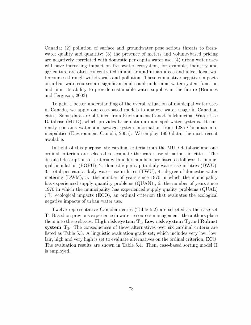
Canada; (2) pollution of surface and groundwater pose serious threats to fresh-water quality and quantity; (3) the presence of meters and volume-based pricingare negatively correlated with domestic per capita water use; (4) urban water useswill have increasing impact on freshwater ecosystem, for example, industry andagriculture are often concentrated in and around urban areas and affect local wa-tercourses through withdrawals and pollution. These cumulative negative impactson urban watercourses are significant and could undermine water system functionand limit its ability to provide sustainable water supplies in the future (Brandesand Ferguson, 2003).
To gain a better understanding of the overall situation of municipal water usesin Canada, we apply our case-based models to analyze water usage in Canadiancities. Some data are obtained from Environment Canada’s Municipal Water UseDatabase (MUD), which provides basic data on municipal water systems. It cur-rently contains water and sewage system information from 1285 Canadian mu-nicipalities (Environment Canada, 2005). We employ 1999 data, the most recentavailable.
In light of this purpose, six cardinal criteria from the MUD database and oneordinal criterion are selected to evaluate the water use situations in cities. Thedetailed descriptions of criteria with index numbers are listed as follows: 1. munic-ipal population (POPU); 2. domestic per capita daily water use in litres (DWU);3. total per capita daily water use in litres (TWU); 4. degree of domestic watermetering (DWM); 5. the number of years since 1970 in which the municipalityhas experienced supply quantity problems (QUAN) ; 6. the number of years since1970 in which the municipality has experienced supply quality problems (QUAL); 7. ecological impacts (ECO), an ordinal criterion that evaluates the ecologicalnegative impacts of urban water use.
Twelve representative Canadian cities (Table 5.2) are selected as the case setT. Based on previous experience in water resources management, the authors placethem into three classes: High risk system T1, Low risk system T2 and Robustsystem T3. The consequences of these alternatives over six cardinal criteria arelisted as Table 5.3. A linguistic evaluation grade set, which includes very low, low,fair, high and very high is set to evaluate alternatives on the ordinal criterion, ECO.The evaluation results are shown in Table 5.4. Then, case-based sorting model IIis employed.
73
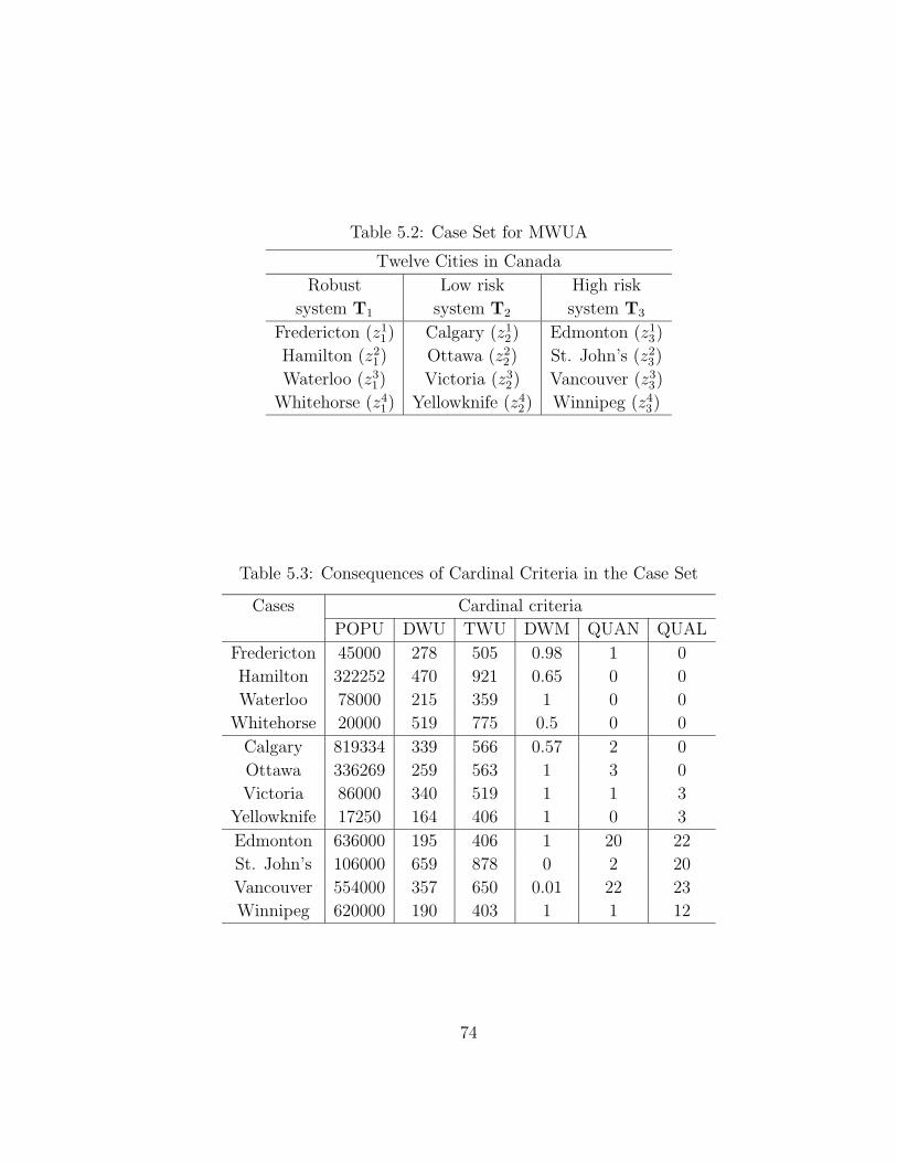
Table 5.2: Case Set for MWUA
Twelve Cities in Canada
Robust Low risk High risk
system T1 system T2 system T3
Fredericton (z11) Calgary (z1
2) Edmonton (z13)
Hamilton (z21) Ottawa (z2
2) St. John’s (z23)
Waterloo (z31) Victoria (z3
2) Vancouver (z33)
Whitehorse (z41) Yellowknife (z4
2) Winnipeg (z43)
Table 5.3: Consequences of Cardinal Criteria in the Case Set
Cases Cardinal criteria
POPU DWU TWU DWM QUAN QUAL
Fredericton 45000 278 505 0.98 1 0
Hamilton 322252 470 921 0.65 0 0
Waterloo 78000 215 359 1 0 0
Whitehorse 20000 519 775 0.5 0 0
Calgary 819334 339 566 0.57 2 0
Ottawa 336269 259 563 1 3 0
Victoria 86000 340 519 1 1 3
Yellowknife 17250 164 406 1 0 3
Edmonton 636000 195 406 1 20 22
St. John’s 106000 659 878 0 2 20
Vancouver 554000 357 650 0.01 22 23
Winnipeg 620000 190 403 1 1 12
74

Table 5.4: Linguistic Evaluations in the Case Set
Cases Ordinal criterion, ECO
Linguistic evaluations Value intervals
Fredericton Very Low [0, 15]
Hamilton Low [15, 2
5]
Waterloo Low [15, 2
5]
Whitehorse Very Low [0, 15]
Calgary Low [15, 2
5]
Ottawa Fair [25, 3
5]
Victoria Fair [25, 3
5]
Yellowknife Low [15, 2
5]
Edmonton High [35, 4
5]
St. John’s High [35, 4
5]
Vancouver Very High [45, 1]
Winnipeg High [35, 4
5]
5.5.2 Sorting Procedures
Firstly the centroid of T1, z+ and the centroid of T3, z− are calculated by Excelusing (5.1) and (5.2), and the results are shown in Table 5.5. The distance betweenzr
g(g = 1, 2, 3; r = 1, 2, 3, 4) and z+ on each criterion are listed in Table 5.6.
Table 5.5: Centroid of the Case Set
Centroid Criteria
POPU DWU TWU DWM QUAN QUAL
z+ 116313 370.5 640 0.7825 0.25 0
z− 479000 350.25 584.25 0.5025 11.25 19.25
The program SOR.2(α, β) is now applied to find R∗ and w∗ for z+ sorting.Note that w = (w1, ..., w7) is the weight vector of the criteria set, POPU, DWU,TWU, DWU, QUAN, QUAL, ECO and R = (R1, R2) is the distance thresholdvector.
75
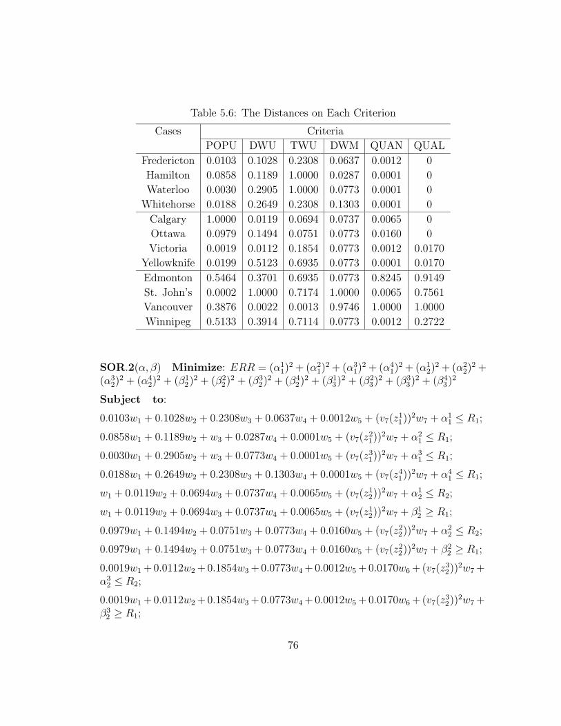
Table 5.6: The Distances on Each Criterion
Cases Criteria
POPU DWU TWU DWM QUAN QUAL
Fredericton 0.0103 0.1028 0.2308 0.0637 0.0012 0
Hamilton 0.0858 0.1189 1.0000 0.0287 0.0001 0
Waterloo 0.0030 0.2905 1.0000 0.0773 0.0001 0
Whitehorse 0.0188 0.2649 0.2308 0.1303 0.0001 0
Calgary 1.0000 0.0119 0.0694 0.0737 0.0065 0
Ottawa 0.0979 0.1494 0.0751 0.0773 0.0160 0
Victoria 0.0019 0.0112 0.1854 0.0773 0.0012 0.0170
Yellowknife 0.0199 0.5123 0.6935 0.0773 0.0001 0.0170
Edmonton 0.5464 0.3701 0.6935 0.0773 0.8245 0.9149
St. John’s 0.0002 1.0000 0.7174 1.0000 0.0065 0.7561
Vancouver 0.3876 0.0022 0.0013 0.9746 1.0000 1.0000
Winnipeg 0.5133 0.3914 0.7114 0.0773 0.0012 0.2722
SOR.2(α, β) Minimize: ERR = (α11)
2 + (α21)
2 + (α31)
2 + (α41)
2 + (α12)
2 + (α22)
2 +(α3
2)2 + (α4
2)2 + (β1
2)2 + (β2
2)2 + (β3
2)2 + (β4
2)2 + (β1
3)2 + (β2
3)2 + (β3
3)2 + (β4
3)2
Subject to:
0.0103w1 + 0.1028w2 + 0.2308w3 + 0.0637w4 + 0.0012w5 + (v7(z11))
2w7 + α11 ≤ R1;
0.0858w1 + 0.1189w2 + w3 + 0.0287w4 + 0.0001w5 + (v7(z21))
2w7 + α21 ≤ R1;
0.0030w1 + 0.2905w2 + w3 + 0.0773w4 + 0.0001w5 + (v7(z31))
2w7 + α31 ≤ R1;
0.0188w1 + 0.2649w2 + 0.2308w3 + 0.1303w4 + 0.0001w5 + (v7(z41))
2w7 + α41 ≤ R1;
w1 + 0.0119w2 + 0.0694w3 + 0.0737w4 + 0.0065w5 + (v7(z12))
2w7 + α12 ≤ R2;
w1 + 0.0119w2 + 0.0694w3 + 0.0737w4 + 0.0065w5 + (v7(z12))
2w7 + β12 ≥ R1;
0.0979w1 + 0.1494w2 + 0.0751w3 + 0.0773w4 + 0.0160w5 + (v7(z22))
2w7 + α22 ≤ R2;
0.0979w1 + 0.1494w2 + 0.0751w3 + 0.0773w4 + 0.0160w5 + (v7(z22))
2w7 + β22 ≥ R1;
0.0019w1 +0.0112w2 +0.1854w3 +0.0773w4 +0.0012w5 +0.0170w6 +(v7(z32))
2w7 +α3
2 ≤ R2;
0.0019w1 +0.0112w2 +0.1854w3 +0.0773w4 +0.0012w5 +0.0170w6 +(v7(z32))
2w7 +β3
2 ≥ R1;
76
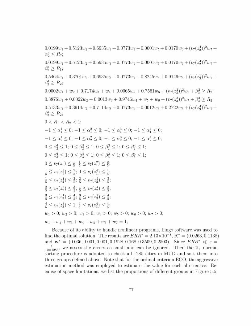
0.0199w1 +0.5123w2 +0.6935w3 +0.0773w4 +0.0001w5 +0.0170w6 +(v7(z42))
2w7 +α4
2 ≤ R2;
0.0199w1 +0.5123w2 +0.6935w3 +0.0773w4 +0.0001w5 +0.0170w6 +(v7(z42))
2w7 +β4
2 ≥ R1;
0.5464w1 +0.3701w2 +0.6935w3 +0.0773w4 +0.8245w5 +0.9149w6 +(v7(z13))
2w7 +β1
3 ≥ R2;
0.0002w1 + w2 + 0.7174w3 + w4 + 0.0065w5 + 0.7561w6 + (v7(z23))
2w7 + β23 ≥ R2;
0.3876w1 + 0.0022w2 + 0.0013w3 + 0.9746w4 + w5 + w6 + (v7(z33))
2w7 + β33 ≥ R2;
0.5133w1 +0.3914w2 +0.7114w3 +0.0773w4 +0.0012w5 +0.2722w6 +(v7(z43))
2w7 +β4
3 ≥ R2;
0 < R1 < R2 < 1;
−1 ≤ α11 ≤ 0; −1 ≤ α2
1 ≤ 0; −1 ≤ α31 ≤ 0; −1 ≤ α4
1 ≤ 0;
−1 ≤ α12 ≤ 0; −1 ≤ α2
2 ≤ 0; −1 ≤ α32 ≤ 0; −1 ≤ α4
2 ≤ 0;
0 ≤ β12 ≤ 1; 0 ≤ β2
2 ≤ 1; 0 ≤ β32 ≤ 1; 0 ≤ β4
2 ≤ 1;
0 ≤ β13 ≤ 1; 0 ≤ β2
3 ≤ 1; 0 ≤ β33 ≤ 1; 0 ≤ β4
3 ≤ 1;
0 ≤ v7(z11) ≤ 1
5; 1
5≤ v7(z
21) ≤ 2
5;
15≤ v7(z
31) ≤ 2
5; 0 ≤ v7(z
41) ≤ 1
5;
15≤ v7(z
12) ≤ 2
5; 2
5≤ v7(z
22) ≤ 3
5;
25≤ v7(z
32) ≤ 3
5; 1
5≤ v7(z
42) ≤ 2
5;
35≤ v7(z
13) ≤ 4
5; 3
5≤ v7(z
23) ≤ 4
5;
45≤ v7(z
33) ≤ 1; 3
5≤ v7(z
43) ≤ 4
5;
w1 > 0; w2 > 0; w3 > 0; w4 > 0; w5 > 0; w6 > 0; w7 > 0;
w1 + w2 + w3 + w4 + w5 + w6 + w7 = 1;
Because of its ability to handle nonlinear programs, Lingo software was used tofind the optimal solution. The results are ERR∗ = 2.13×10⁻⁸, R∗ = (0.0263, 0.1138)and w∗ = (0.036, 0.001, 0.001, 0.1928, 0.168, 0.3509, 0.2503). Since ERR∗ ≪ ε =
110×1285
, we assess the errors as small and can be ignored. Then the z+ normalsorting procedure is adopted to check all 1285 cities in MUD and sort them intothree groups defined above. Note that for the ordinal criterion ECO, the aggressiveestimation method was employed to estimate the value for each alternative. Be-cause of space limitations, we list the proportions of different groups in Figure 5.5.
77
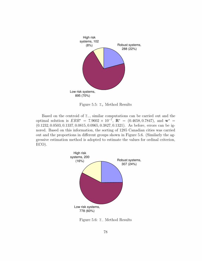
Low risk systems,
895 (70%)
Robust systems,
288 (22%)
High risk
systems, 102
(8%)
Figure 5.5: z+ Method Results
Based on the centroid of z−, similar computations can be carried out and theoptimal solution is ERR∗ = 7.9602 × 10⁻⁷, R∗ = (0.4658, 0.7847), and w∗ =(0.1232, 0.0503, 0.1337, 0.0815, 0.0965, 0.3827, 0.1321). As before, errors can be ig-nored. Based on this information, the sorting of 1285 Canadian cities was carriedout and the proportions in different groups shown in Figure 5.6. (Similarly the ag-gressive estimation method is adopted to estimate the values for ordinal criterion,ECO).
Low risk systems,
778 (60%)
Robust systems,
307 (24%)
High risk
systems, 200
(16%)
Figure 5.6: z− Method Results
78
As seen in Figures 5.5 and 5.6, ρ1, ρ2, ρ3 for the z+ sorting method are 22%, 70%,8% and ρ1, ρ2, ρ3 for z− sorting method are 24%, 60%, 16%, respectively. Therefore,Φ+ = (ρ2, ρ1, ρ3) = Φ−, thus T provides roughly consistent results by both z+ andz− sorting methods. We conclude that based on our current information (knowl-edge), the water supply systems in most Canadian cities are robust or low risk,so the overall situation is still acceptable. However, water use in Canadian citiesis typically twice as great as European cities, which suggests that great potentialexists to reduce the volume of water use by Canadian cities with minimal impactson quality of life standard. It has been argued that curbing the trend of increasingwater use can provide significant ecological, social and economic benefits (Brandesand Ferguson, 2003).
5.6 Conclusions
Case-based distance methods are proposed in this chapter to solve sorting problemsin MCDA. The main components of the chapters are:
• General description of sorting problems: A formal definition of sorting prob-lems is presented and the relationship between A, the alternative set, and S,the sorting group, is discussed.
• Case-based sorting model I: The method is designed for sorting problemshaving cardinal criteria.
• Case-based sorting model II: This method is an extension of case-based sortingmodel I and can handle both cardinal and ordinal criteria.
• Case study: An application to municipal water usage in Canada is presented.
79
Chapter 6
Sorting Problem Application inInventory Management
6.1 Introduction
In ABC analysis, a well-known inventory planning and control technique, stock-keeping units (SKUs) are sorted into three categories. Traditionally, the sorting isbased solely on annual dollar usage. The aim of this chapter is to introduce a case-based multiple criteria ABC analysis (MCABC) that improves on this approachby accounting for additional criteria, such as lead time and criticality of SKUs,thereby providing more managerial flexibility. Firstly, the motivation of MCABCis explained briefly. Next, research on ABC analysis and its extension, MCABCis explained in detail. Then, a case-based distance method is proposed to solveMCABC problems. Finally, a case study is developed to illustrate how the proce-dure can be applied; the results demonstrate that this approach is robust and canproduce sound classifications of SKUs when multiple criteria are to be considered.The contents of this chapter is based on research by Chen et al. (2005e).
6.2 Motivation
Efficient and effective inventory management assumes increasing significance inmaintaining a firm’s competitive advantage with the acceleration of globalizationof businesses (Silver et al., 1998). Generally, the number of SKUs in a firm caneasily go up to tens of thousands or even more. Therefore, it is not economically
80
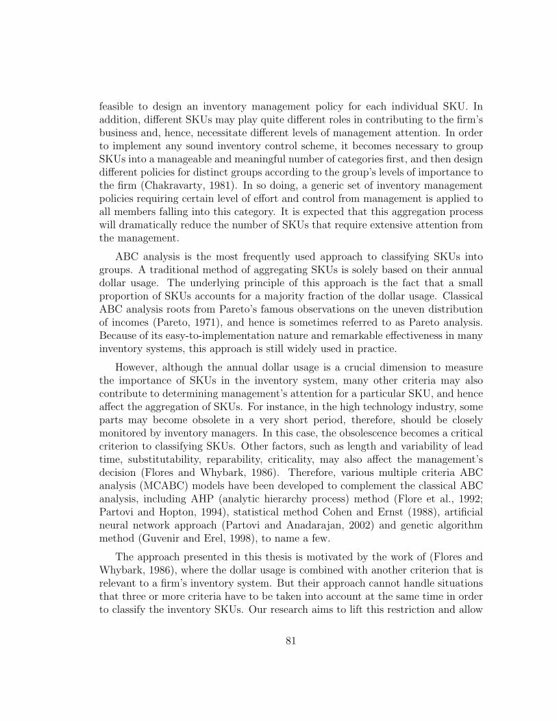
feasible to design an inventory management policy for each individual SKU. Inaddition, different SKUs may play quite different roles in contributing to the firm’sbusiness and, hence, necessitate different levels of management attention. In orderto implement any sound inventory control scheme, it becomes necessary to groupSKUs into a manageable and meaningful number of categories first, and then designdifferent policies for distinct groups according to the group’s levels of importance tothe firm (Chakravarty, 1981). In so doing, a generic set of inventory managementpolicies requiring certain level of effort and control from management is applied toall members falling into this category. It is expected that this aggregation processwill dramatically reduce the number of SKUs that require extensive attention fromthe management.
ABC analysis is the most frequently used approach to classifying SKUs intogroups. A traditional method of aggregating SKUs is solely based on their annualdollar usage. The underlying principle of this approach is the fact that a smallproportion of SKUs accounts for a majority fraction of the dollar usage. ClassicalABC analysis roots from Pareto’s famous observations on the uneven distributionof incomes (Pareto, 1971), and hence is sometimes referred to as Pareto analysis.Because of its easy-to-implementation nature and remarkable effectiveness in manyinventory systems, this approach is still widely used in practice.
However, although the annual dollar usage is a crucial dimension to measurethe importance of SKUs in the inventory system, many other criteria may alsocontribute to determining management’s attention for a particular SKU, and henceaffect the aggregation of SKUs. For instance, in the high technology industry, someparts may become obsolete in a very short period, therefore, should be closelymonitored by inventory managers. In this case, the obsolescence becomes a criticalcriterion to classifying SKUs. Other factors, such as length and variability of leadtime, substitutability, reparability, criticality, may also affect the management’sdecision (Flores and Whybark, 1986). Therefore, various multiple criteria ABCanalysis (MCABC) models have been developed to complement the classical ABCanalysis, including AHP (analytic hierarchy process) method (Flore et al., 1992;Partovi and Hopton, 1994), statistical method Cohen and Ernst (1988), artificialneural network approach (Partovi and Anadarajan, 2002) and genetic algorithmmethod (Guvenir and Erel, 1998), to name a few.
The approach presented in this thesis is motivated by the work of (Flores andWhybark, 1986), where the dollar usage is combined with another criterion that isrelevant to a firm’s inventory system. But their approach cannot handle situationsthat three or more criteria have to be taken into account at the same time in orderto classify the inventory SKUs. Our research aims to lift this restriction and allow
81

any finite number of criteria to be considered simultaneously.
6.3 Multiple Criteria ABC Analysis (MCABC)
Classical ABC analysis aggregates SKUs into different groups based solely on theannual dollar usage. The most important SKUs in terms of dollar usage are placedin group A, which demand the greatest effort and attention from the management;the least important SKUs are aggregated into group C, which are given the minimalcontrol; other SKUs are categorized into group B, on which medium level of controlis exerted. The “80-20 (or 90-10) Rule” — 80% (or 90%) of the total annual usagecomes from 20% (or 10%) of SKUs — constitutes the basis of the classical ABCanalysis. The rule guarantees that the number of A SKUs is substantially smallerthan the total number of SKUs in the inventory system. Although the exact valuesvary from industry to industry, the 80-20 rule can be applied to many real-worldsituations. Figure 6.1 captures the essence of this rule. Note that A represents theset of alternatives, {A1, A2, · · · , Ai, · · · , An}. Q = {1, 2, · · · , j, · · · , q} is the set ofcriteria. The consequence on criterion j of alternative Ai is expressed as cj(A
i).
Cumulative percentage of dollar usage
Cumulative percentage of SKUs
80%
20%
Figure 6.1: Example of Dollar Usage Distribution Curve
The classification obtained from the ABC analysis is sometimes subject to fur-ther adjustments, for example, some SKUs’ dollar usages may not be so significant,but their stock-out cost can be unbearably high; while some other SKUs may havehigh dollar usages, but their supply is sufficient and consistent. In these cases,
82
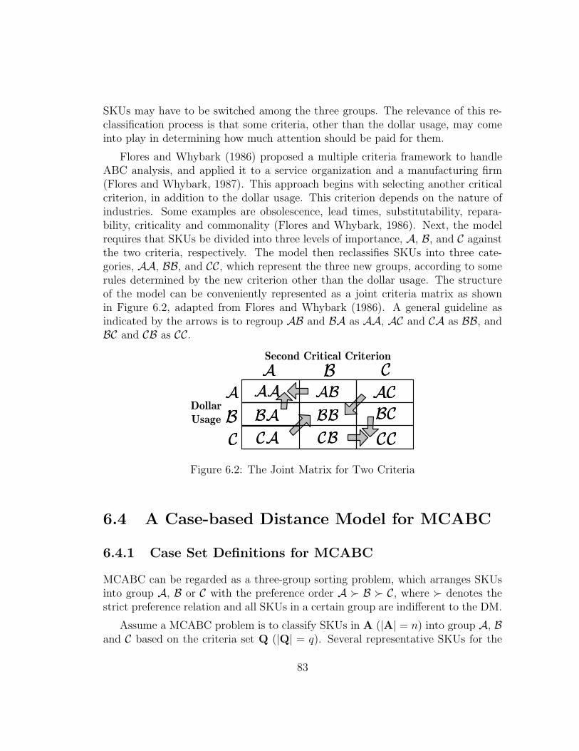
SKUs may have to be switched among the three groups. The relevance of this re-classification process is that some criteria, other than the dollar usage, may comeinto play in determining how much attention should be paid for them.
Flores and Whybark (1986) proposed a multiple criteria framework to handleABC analysis, and applied it to a service organization and a manufacturing firm(Flores and Whybark, 1987). This approach begins with selecting another criticalcriterion, in addition to the dollar usage. This criterion depends on the nature ofindustries. Some examples are obsolescence, lead times, substitutability, repara-bility, criticality and commonality (Flores and Whybark, 1986). Next, the modelrequires that SKUs be divided into three levels of importance, A, B, and C againstthe two criteria, respectively. The model then reclassifies SKUs into three cate-gories, AA, BB, and CC, which represent the three new groups, according to somerules determined by the new criterion other than the dollar usage. The structureof the model can be conveniently represented as a joint criteria matrix as shownin Figure 6.2, adapted from Flores and Whybark (1986). A general guideline asindicated by the arrows is to regroup AB and BA as AA, AC and CA as BB, andBC and CB as CC.
Dollar
Usage
Second Critical Criterion
AA
BB
CC
AA BB
AAAA
BBBB
CCCC
ABAB
CC
ACAC
BABA
CACA
BCBC
CBCB
Figure 6.2: The Joint Matrix for Two Criteria
6.4 A Case-based Distance Model for MCABC
6.4.1 Case Set Definitions for MCABC
MCABC can be regarded as a three-group sorting problem, which arranges SKUsinto group A, B or C with the preference order A ≻ B ≻ C, where ≻ denotes thestrict preference relation and all SKUs in a certain group are indifferent to the DM.
Assume a MCABC problem is to classify SKUs in A (|A| = n) into group A, Band C based on the criteria set Q (|Q| = q). Several representative SKUs for the
83

MCABC problem are available and they are partitioned into three categories TA,TB, and TC which represent case sets for groups A, B, and C, respectively. Thenumber of SKUs in group g (g = A,B, C) is denoted ng and zr
g is a representativeSKU in Tg. The SKUs in case sets may, for example, be fabricated by the DMor obtained by having the DM modify historical records and the case sets arecomprehensive representative for the DM. Note that all criteria in Q must apply andcj(A
i) must be measurable for all SKUs in the case sets and all j ∈ Q. Preferenceand indifference of SKUs are induced in the case sets. For two SKUs in the samegroup, they are equally preferred by the DM. For example, zk
B, zlB ∈ TB, zk
B ∼ zlB
(∼ means the DM equally prefers zkg and zl
g); any SKU in a more important groupis more preferred to the one in a less important group. For example, zk
A ∈ TA, andzlB ∈ TB, zk
A ≻ zlB.
Our case-based reasoning idea is based on the “right” distance based preferenceexpression: the distances of cases to a pre-defined point in the same group shouldbe close together within a range and farther from the distances of cases in othergroups in some sense. We use Tg, g = A,B, C, to estimate criterion weight w,and a distance threshold vector R, so that this information can be applied toclassify (sort) SKUs in A. Figure 6.3 demonstrates one situation of this idea. Twoellipses partition the SKUs into three case sets and represent preference sequences:ellipses closer to “o” represent more preferred groups. For zr
A ∈ TA, zrB ∈ TB
and zrC ∈ TC, zr
A ≻ zrB ≻ zr
C. Then by a properly designed transformation fromthe original consequence data space to a weighted normalized consequence dataspace (preference space), ellipse-based distances can be transformed to circle-baseddistances and accordingly this information can be applied to classify SKUs in A.Notice that in Figure 6.3 the distance of zr
A from “o” is less than RA, the distanceof zr
B is greater than RA and less than RB, and the distance of zrC is greater than
RB.
6.4.2 Distance Assumptions
Assuming the DM’s preferences over Q are monotonic and two kinds of criteria aredefined as follows: (1) benefit criteria, Q+, which mean the greater value (conse-quences) the more important (preference) for the DM; (2) cost criteria, Q−, whichmean the less value (consequences) the more important (preference) for the DM.Thus, Q = Q+ ∪Q−. For example, the manager in a manufacturing company mayset the criterion of dollar usage as Q+ while the criterion of lead time as Q−. Fur-thermore, the DM can identify the maximum consequence on criterion j (j ∈ Q),cmaxj ∈ R+ and the minimum consequence, cmin
j ∈ R+ , where cmaxj > cmin
j . Notice
84
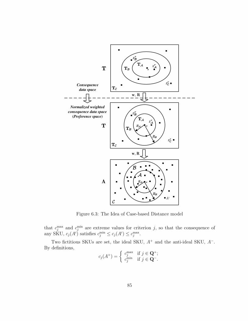
Normalized weighted
consequence data space
(Preference space)
w, R
.
.
.
.
.
.
o.
o. .
.
.
.
.
.
..
.
w, R
A o. .
.
.
.
.
.
.
.
.
.
.
.
.
.
.
.
.
.
.
.
.
.
.
.
..
.
.
Ai
.
.
.
.
..
.
.
.
. .
.
.
.
.
.
Consequence
data space
.
.
TATA
TATA
TT
TT
TBTB
TCTC
TCTC
TBTB
zrCzrC
zrCzrC
zrAzrA
zrAzrA
zrBzrB
zrBzrB
RARA
RBRB
RBRB
RARA
BB
AA
CC
Figure 6.3: The Idea of Case-based Distance model
that cmaxj and cmin
j are extreme values for criterion j, so that the consequence ofany SKU, cj(A
i) satisfies cminj ≤ cj(A
i) ≤ cmaxj .
Two fictitious SKUs are set, the ideal SKU, A+ and the anti-ideal SKU, A−.By definitions,
cj(A+) =
{
cmaxj if j ∈ Q+;
cminj if j ∈ Q−.
85
and
cj(A−) =
{
cminj if j ∈ Q+;
cmaxj if j ∈ Q−.
For j = 1, 2, ..., q, define dmaxj =
(
cmaxj −cmin
j
)2to be the normalization factor for
criterion j. For g = A,B, C and r = 1, 2, ..., ng, the normalized distance betweenzr
g ∈ Tg and A+ on criterion j is
dj(zrg , A
+) = dj(zrg)
+ =
(
cj(zrg) − cj(A
+))2
dmaxj
. (6.1)
Note that (6.1) defines dj(Ai)+ if Ai = zr
g , Ai ∈ A. Similarly, the distance betweenany SKU zr
g ∈ Tg and A− on criterion j is
dj(zrg , A
−) = dj(zrg)
− =
(
cj(zrg) − cj(A
−))2
dmaxj
. (6.2)
Note that (6.2) defines dj(Ai)− if if Ai = zr
g , Ai ∈ A. It is easy to verify thatdj(z
rg)
+ ∈ [0, 1], dj(Ai)+ ∈ [0, 1], dj(z
rg)
− ∈ [0, 1], and dj(Ai)− ∈ [0, 1].
The aggregated distance between zrg ∈ Tg and A+ over the criteria set Q is
identified asD(zr
g , A+) = D(zr
g)+ =
∑
j∈Q
w+j · dj(z
rg)
+, (6.3)
where w+j ∈ w+ is the A+-based weight (relative importance) of criterion j. The
weight vector w+ is to be determined. It is assumed that 0 < w+j ≤ 1 and
∑
j∈Q
w+j =
1. Similarly, the aggregated distance from alternative zrg to A− is
D(zrg , A
−) = D(zrg)
− =∑
j∈Q
w−j · dj(z
rg)
−, (6.4)
where w−j ∈ w− is the A−-based weight of criterion j. Note that (6.3) and (6.4)
define D(Ai)+ and D(Ai)−, respectively, if Ai = zrg , Ai ∈ A.
6.4.3 Model Construction
Taking A+ as the original point “o”, A+MCABC analysis is explained as follows:a compact ball (in q dimensions) with radius of R+
A ∈ R+ includes (in principle)every case in TA and any case that is not in TA is (in principle) outside that ball.
86
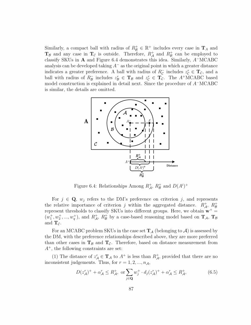
Similarly, a compact ball with radius of R+B ∈ R+ includes every case in TA and
TB and any case in TC is outside. Therefore, R+A and R+
B can be employed toclassify SKUs in A and Figure 6.4 demonstrates this idea. Similarly, A−MCABCanalysis can be developed taking A− as the original point in which a greater distanceindicates a greater preference. A ball with radius of R−
C includes zrC ∈ TC, and a
ball with radius of R−B includes zr
B ∈ TB and zrC ∈ TC. The A+MCABC based
model construction is explained in detail next. Since the procedure of A−MCABCis similar, the details are omitted.
A .
.
.
.
.
.
.
..
.
.
.
.
.
..
.
.
.
.
.
.
.
.
.
.
.
.
.
.
.
.
A+
Distance
.
A+
D(Ai)+
Ai
CC
AA
BB
R+
AR+
A
R+
BR+
B
Figure 6.4: Relationships Among R+A, R+
B and D(Ai)+
For j ∈ Q, wj refers to the DM’s preference on criterion j, and representsthe relative importance of criterion j within the aggregated distance. R+
A, R+B
represent thresholds to classify SKUs into different groups. Here, we obtain w+ =(w+
1 , w+2 , ..., w+
q ), and R+A, R+
B by a case-based reasoning model based on TA, TB
and TC.
For an MCABC problem SKUs in the case set TA (belonging to A) is assessed bythe DM, with the preference relationships described above, they are more preferredthan other cases in TB and TC. Therefore, based on distance measurement fromA+, the following constraints are set:
(1) The distance of zrA ∈ TA to A+ is less than R+
A, provided that there are noinconsistent judgements. Thus, for r = 1, 2, ..., nA,
D(zrA)+ + αr
A ≤ R+A, or
∑
j∈Q
w+j · dj(z
rA)+ + αr
A ≤ R+A, (6.5)
87
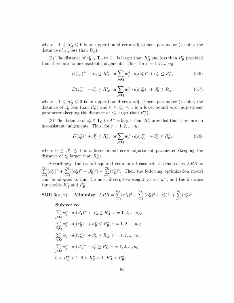
where −1 ≤ αrA ≤ 0 is an upper-bound error adjustment parameter (keeping the
distance of zrA less than R+
A).
(2) The distance of zrB ∈ TB to A+ is larger than R+
A and less than R+B provided
that there are no inconsistent judgements. Thus, for r = 1, 2, ..., nB,
D(zrB)+ + αr
B ≤ R+B , or
∑
j∈Q
w+j · dj(z
rB)+ + αr
B ≤ R+B , (6.6)
D(zrB)+ + βr
B ≥ R+A, or
∑
j∈Q
w+j · dj(z
rB)+ + βr
B ≥ R+A, (6.7)
where −1 ≤ αrB ≤ 0 is an upper-bound error adjustment parameter (keeping the
distance of zrB less than R+
B ) and 0 ≤ βrB ≤ 1 is a lower-bound error adjustment
parameter (keeping the distance of zrB larger than R+
A).
(3) The distance of zrC ∈ TC to A+ is larger than R+
B provided that there are noinconsistent judgements. Thus, for r = 1, 2, ..., nC,
D(zrC)
+ + βrC ≥ R+
B , or∑
j∈Q
w+j · dj(z
rC)
+ + βrC ≥ R+
B , (6.8)
where 0 ≤ βrC ≤ 1 is a lower-bound error adjustment parameter (keeping the
distance of zrC larger than R+
B ).
Accordingly, the overall squared error in all case sets is denoted as ERR =nA∑
r=1
(αrA)2 +
nB∑
r=1
[(αrB)2 + βr
B)2] +nC∑
r=1
(βrC)
2. Then the following optimization model
can be adopted to find the most descriptive weight vector w+, and the distancethresholds R+
A and R+B .
SOR.3(α, β) Minimize : ERR =nA∑
r=1
(αrA)2 +
nB∑
r=1
[(αrB)2 + βr
B)2] +nC∑
r=1
(βrC)
2
Subject to:∑
j∈Q
w+j · dj(z
rA)+ + αr
A ≤ R+A, r = 1, 2, ..., nA;
∑
j∈Q
w+j · dj(z
rB)+ + αr
B ≤ R+B , r = 1, 2, ..., nB;
∑
j∈Q
w+j · dj(z
rB)+ + βr
B ≥ R+A, r = 1, 2, ..., nB;
∑
j∈Q
w+j · dj(z
rC)
+ + βrC ≥ R+
B , r = 1, 2, ..., nC;
0 < R+A < 1, 0 < R+
B < 1, R+A < R+
B ;
88

−1 ≤ αrg ≤ 0, g = A,B;
0 ≤ βrg ≤ 1, g = B, C;
w+j > 0,
∑
j∈Q
w+j = 1;
Theorem 6. SOR.3(α, β) has at least one optimal solution.
Proof: The constraints in SOR.3(α, β) constitute a convex set. The objectivefunction ERR is a quadratic function on this set. Based on the extreme valuetheorem of advanced calculus (Fitzpatrick, 1995, page 297), the function ERRis continuous and the set of all possible variables is bounded, ERR attains itsminimum at least once. ¤
An indifference distance threshold, ε is set to evaluate the error, ERR, generatedby SOR.3(α, β): When ERR ≤ ε, the error is small and can be ignored, so theinformation in the case sets provided by the DM is considered to be consistent;when ERR > ε, the error cannot be ignored and there is some inconsistency in thecase sets. The DM should reconsider them. A suggested value of ε is 1
kn, n = |A|,
where k ∈ R+ is the adjustment parameter. When the case set is large and thelikelihood of the error is high, then k < 1; when the case set is small and thelikelihood of the error is small, then k ≥ 1.
Furthermore, to make the optimal results more closely reflect a DM’s intrinsicpreferences, the DM could provide some rough information about weights and in-corporate it into SOR.3(α, β). The imprecise preference expressions proposed bySage and White (1984), and Eum et al. (2001) can be used for this purpose. Someimprecise weight preference expressions are listed below:
• Weak ranking: w1 ≥ w2 ≥ · · · ≥ wq > 0;
• Strict ranking: wj − wj+1 ≥ ǫj, j ∈ Q, where ǫj is a small positive value;
• Difference ranking: w1 − w2 ≥ · · · ≥ wq−1 − wq ≥ 0;
• Fixed bounds: Lj ≤ wj ≤ Uj, j ∈ Q, where Lj and Uj are lower and upperbounds for wj, respectively;
The following imprecise weight preference expressions are proposed to align withthe MCABC scenario:
wd ≥ wk,∀ k ∈ Q, k 6= d (6.9)
Lj ≤ wj ≤ Uj, ∀ j ∈ Q (6.10)
89
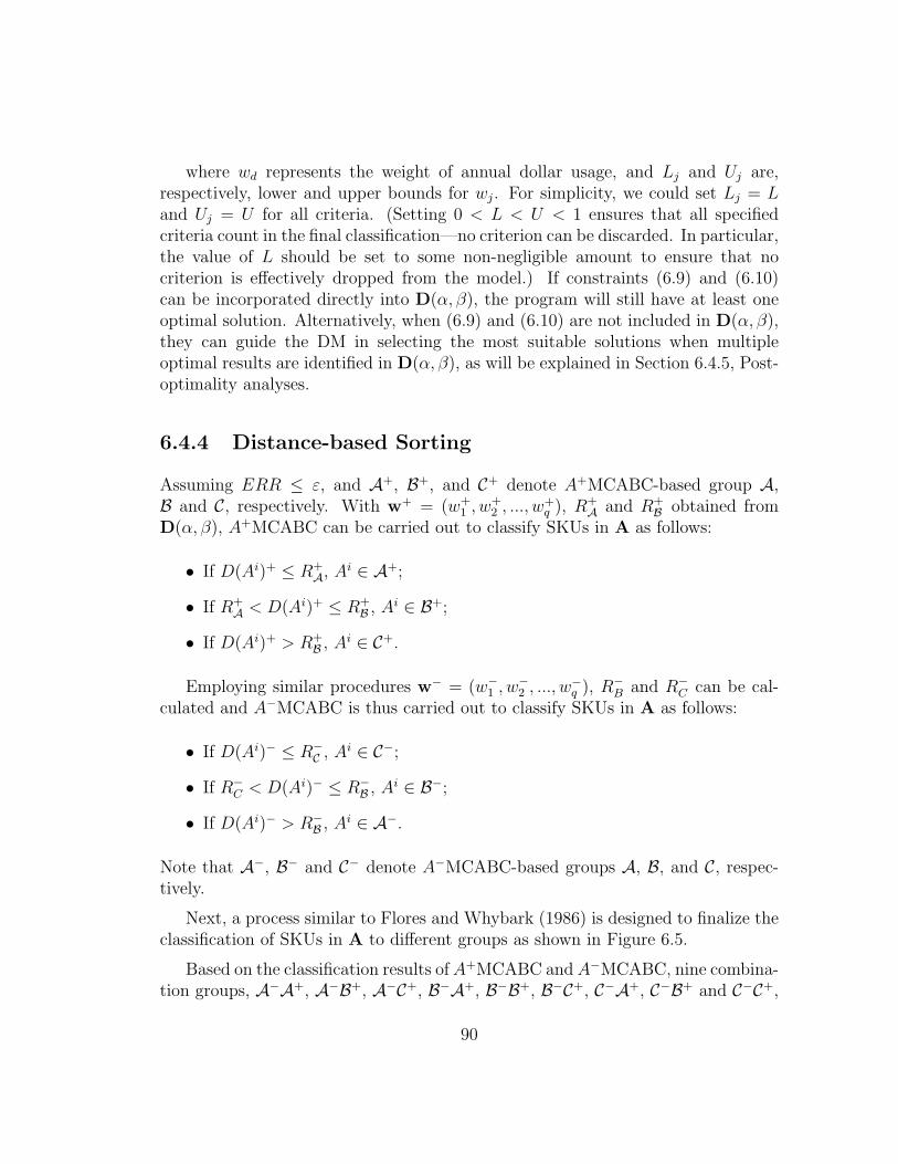
where wd represents the weight of annual dollar usage, and Lj and Uj are,respectively, lower and upper bounds for wj. For simplicity, we could set Lj = Land Uj = U for all criteria. (Setting 0 < L < U < 1 ensures that all specifiedcriteria count in the final classification—no criterion can be discarded. In particular,the value of L should be set to some non-negligible amount to ensure that nocriterion is effectively dropped from the model.) If constraints (6.9) and (6.10)can be incorporated directly into D(α, β), the program will still have at least oneoptimal solution. Alternatively, when (6.9) and (6.10) are not included in D(α, β),they can guide the DM in selecting the most suitable solutions when multipleoptimal results are identified in D(α, β), as will be explained in Section 6.4.5, Post-optimality analyses.
6.4.4 Distance-based Sorting
Assuming ERR ≤ ε, and A+, B+, and C+ denote A+MCABC-based group A,B and C, respectively. With w+ = (w+
1 , w+2 , ..., w+
q ), R+A and R+
B obtained fromD(α, β), A+MCABC can be carried out to classify SKUs in A as follows:
• If D(Ai)+ ≤ R+A, Ai ∈ A+;
• If R+A < D(Ai)+ ≤ R+
B , Ai ∈ B+;
• If D(Ai)+ > R+B , Ai ∈ C+.
Employing similar procedures w− = (w−1 , w−
2 , ..., w−q ), R−
B and R−C can be cal-
culated and A−MCABC is thus carried out to classify SKUs in A as follows:
• If D(Ai)− ≤ R−C , Ai ∈ C−;
• If R−C < D(Ai)− ≤ R−
B , Ai ∈ B−;
• If D(Ai)− > R−B , Ai ∈ A−.
Note that A−, B− and C− denote A−MCABC-based groups A, B, and C, respec-tively.
Next, a process similar to Flores and Whybark (1986) is designed to finalize theclassification of SKUs in A to different groups as shown in Figure 6.5.
Based on the classification results of A+MCABC and A−MCABC, nine combina-tion groups, A−A+, A−B+, A−C+, B−A+, B−B+, B−C+, C−A+, C−B+ and C−C+,
90
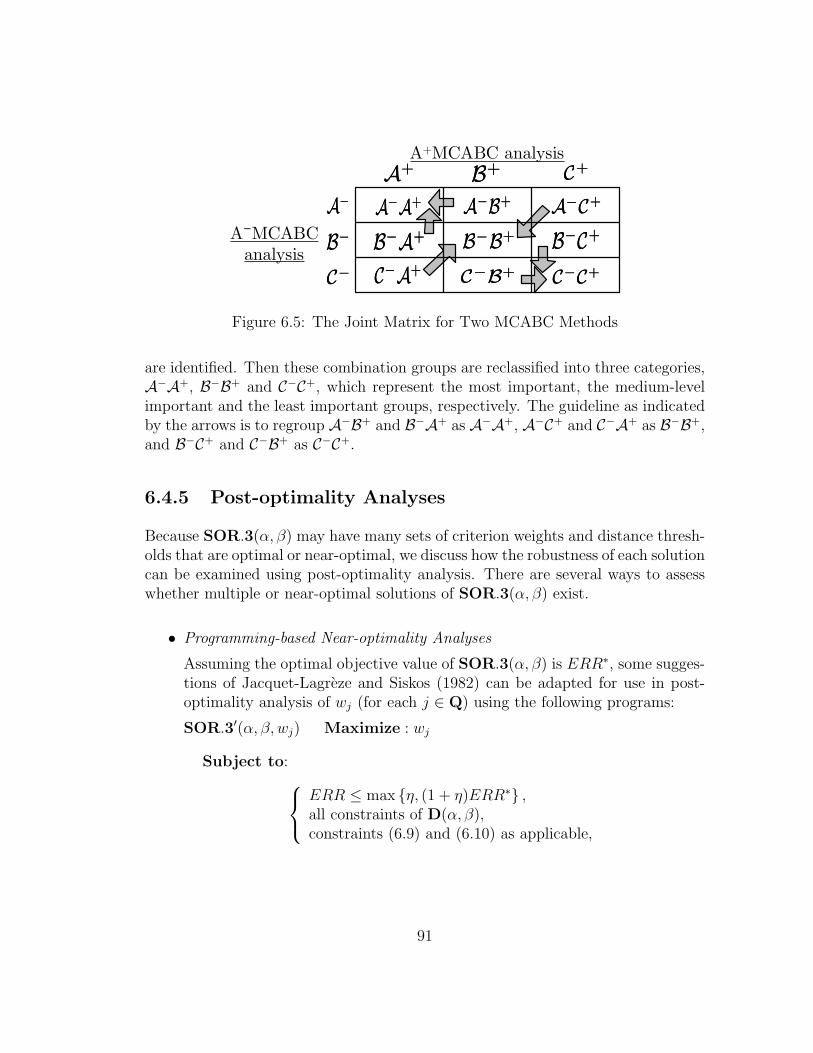
A+MCABC analysis
A¯MCABC
analysis
B+B+A+A+ C+C+
CC
BB
AA A A+A A+ A B+A B+ A C+A C+
B A+B A+
C A+C A+
B B+B B+
C B+C B+ C C+C C+
B C+B C+
Figure 6.5: The Joint Matrix for Two MCABC Methods
are identified. Then these combination groups are reclassified into three categories,A−A+, B−B+ and C−C+, which represent the most important, the medium-levelimportant and the least important groups, respectively. The guideline as indicatedby the arrows is to regroup A−B+ and B−A+ as A−A+, A−C+ and C−A+ as B−B+,and B−C+ and C−B+ as C−C+.
6.4.5 Post-optimality Analyses
Because SOR.3(α, β) may have many sets of criterion weights and distance thresh-olds that are optimal or near-optimal, we discuss how the robustness of each solutioncan be examined using post-optimality analysis. There are several ways to assesswhether multiple or near-optimal solutions of SOR.3(α, β) exist.
• Programming-based Near-optimality Analyses
Assuming the optimal objective value of SOR.3(α, β) is ERR∗, some sugges-tions of Jacquet-Lagreze and Siskos (1982) can be adapted for use in post-optimality analysis of wj (for each j ∈ Q) using the following programs:
SOR.3′(α, β, wj) Maximize : wj
Subject to:
ERR ≤ max {η, (1 + η)ERR∗} ,all constraints of D(α, β),constraints (6.9) and (6.10) as applicable,
91

SOR.3′′(α, β, wj) Minimize : wj
Subject to:
ERR ≤ max {η, (1 + η)ERR∗} ,all constraints of D(α, β),constraints (6.9) and (6.10) as applicable,
In both programs, η is a small positive number.
These programs obtain maximum and minimum values for wj. Similarly,the programs SOR.3′(α, β,R+
A), SOR.3′(α, β,R+B ), SOR.3′′(α, β,R+
A) andSOR.3′′(α, β,R+
B ) yield, respectively, maximum and minimum values for R+A
and R+B . The difference between the generated minimum and maximum values
for a criterion weight or distance threshold is a measure of the robustness ofthe initial solution.
There are two ways to use this robustness information to determine a finalsorting.
1. Average Value Method: Based on the suggestions from Jacquet-Lagrezeand Siskos (1982) and Siskos et al. (2005), the averages of the initialsolutions, and the maximum and minimum values for each criterion ordistance threshold generated from the above procedures may be consid-ered as a more representative solution of D(α, β), and used to sort SKUs.
2. Percentage Value Method: Each of SOR.3(α, β), SOR.3′(α, β,R+A),
SOR.3′(α, β,R+B ), SOR.3′′(α, β,R+
A) and SOR.3′′(α, β,R+B ) generates
a vector of solutions for all criterion weights and distance thresholds.Each of these vectors implies a different sorting of the SKUs. For eachSKU, the frequency of sorting into A, B and C can be calculated. (Asharply peaked distribution is another indicator of robustness.) Theneach SKU is assigned to the group where it appears most often, for bothA+MCABC and A−MCABC. Finally, the procedure explained in Figure6.5 is applied to generate the final sorting result.
• Multiple Optimal Solution Identification and Selection
Another way to conduct the post-optimality analyses is to employ optimiza-tion software packages, such as LINGO and Matlab, in which varying the
92
initialization of the optimization algorithm can identify multiple optimal so-lutions. When SOR.3(α, β) has multiple solutions, the DM could select asolution which is in some sense “closest” to the imprecise weight informationhe or she has supplied, as in (6.9) and (6.10). For example, solutions that donot satisfy the constraint (6.9) can simply be screened out. Also, the meanof the two parameters of (6.10), (L + U)/2, can be employed as a centroid—in which case, the solution at minimum distance from the centroid shouldbe regarded as best. Notice that (6.9) and (6.10) are not incorporated intoSOR.3(α, β) as constraints.
• Transformation of the Objective Function
The sum of squared errors,nA∑
r=1
(αrA)2 +
nB∑
r=1
[(αrB)2 + (βr
B)2] +nC∑
r=1
(βrC)
2, the ob-
jective function in SOR.3(α, β), measures the overall error in representationof the entire case set. Because it is similar to linear regression in statis-tics, this representation may be easily understood by DMs. Nevertheless,there are other ways to express the overall error. For instance, followingthe example of Siskos and Yannacopoulos (1985) and Siskos et al. (2005),nA∑
r=1
(−αrA)+
nB∑
r=1
[(−αrB)+βr
B]+nC∑
r=1
(βrC) also measures the overall error. In other
words, this procedure transforms SOR.3(α, β) is transformed into a linearrather than a quadratic program. The same procedures described by Siskoset al. (2005) can then be employed to carry out post-optimality analyses. Theconstraints (6.9) and (6.10) may be incorporated in SOR.3(α, β), dependingon the DM’s available information.
6.5 A Case Study in Hospital Inventory Manage-
ment
6.5.1 Background
A case study to demonstrate the proposed procedure is carried out based upondata in Flore et al. (1992) on a hospital inventory management. In that example,47 disposable SKUs used in a hospital-based respiratory therapy unit are classifiedusing the AHP (Saaty, 1980) based MCABC. Table 6.1 lists the 47 disposable SKUsreferred to as S1 through S47. Four criteria are defined for MCABC analysis: (1)average unit cost ($), which ranges from a low $5.12 to a high of $210.00; (2) annual
93
dollar usage ($), which ranges from $25.38 to a high of $5840.64; (3) critical factor,1, 0.50, or 0.01 is assigned to the 47 disposable SKUs. A value of 1 indicates verycritical, a value of 0.50 indicates moderately critical and a value of 0.01 for non-critical; (4) lead time (week) is the time it takes to receive replenishment after it isordered, ranging from 1 to 7 weeks.
6.5.2 Selection of Case Sets
In this case study, all criteria are assumed to be positive criteria, which meansthe greater value of the consequence, the more important it is for the DM. Notethat for a product buyer, like hospitals, lead time is a positive criterion while fora producer it may be a negative criterion. The settings of A+, A− are listed inTable 6.2. It is assumed that the DM would like to provide the case information,three representative SKUs for A, four for B, and four for C among those 47 SKUs.We start with the most representative case set as shown in Table 6.2. Based onthis information, the normalized consequence data of case sets for A+MCABC andA−MCABC are calculated using (6.1) and (6.2), and listed in Tables 6.3 and 6.4,respectively.
Based on this information, the normalized consequence data of case sets forA+MCABC and A−MCABC are calculated using (6.1) and (6.2), and listed inTable 6.3, and 6.4, respectively.
6.5.3 Model Construction
First, SOR.3(α, β) is employed to find w+ = {w+1 , w+
2 , w+3 , w+
4 } as well as R+A
and R+B , which represent the weights for the average unit cost, the annual dollar
usage, the critical factor, the lead time, and the distance thresholds for A and Bin A+ABC, respectively. The imprecise weight information is assumed to be asfollows: for j = 1, 2, 3, 4, 0.01 ≤ w+
j ≤ 0.9; w+2 ≥ w+
1 ; w+2 ≥ w+
3 ; w+2 ≥ w+
4 .These two groups of constraints guarantee that each weight is positive and hencethat each criterion contributes to the classification, and that the dollar usage is themost important criterion.
The results found using Lingo software (Lingo, 2005) are ERR = 1.1878×10⁻⁹;w+ = (0.0915, 0.3118, 0.2987, 0.2980), R+
A = 0.2700 and R+B = 0.6717. Assuming
ε = 1n
= 147
, since ε ≪ ERR, the error can be ignored.
The optimization problem is:Minimize : ERR = (α1
A)2 +(α2A)2 +(α3
A)2 +(α1B)2 +(α2
B)2 +(α3B)2 +(α4
B)2 +(β1B)2 +
94
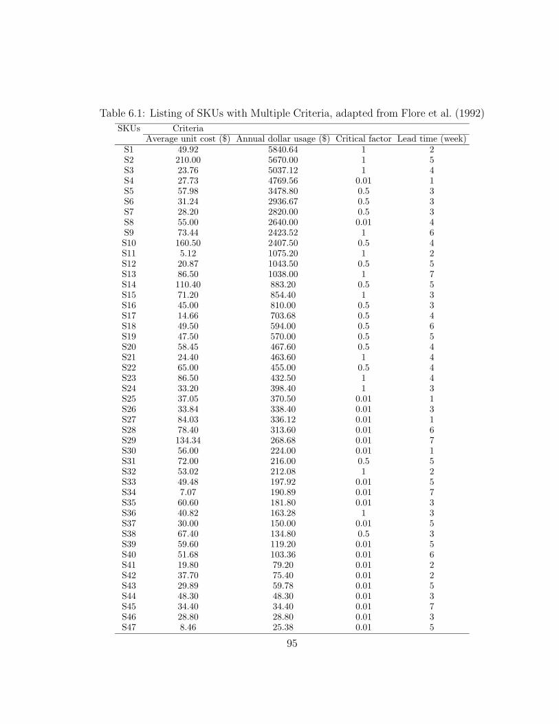
Table 6.1: Listing of SKUs with Multiple Criteria, adapted from Flore et al. (1992)
SKUs CriteriaAverage unit cost ($) Annual dollar usage ($) Critical factor Lead time (week)
S1 49.92 5840.64 1 2S2 210.00 5670.00 1 5S3 23.76 5037.12 1 4S4 27.73 4769.56 0.01 1S5 57.98 3478.80 0.5 3S6 31.24 2936.67 0.5 3S7 28.20 2820.00 0.5 3S8 55.00 2640.00 0.01 4S9 73.44 2423.52 1 6S10 160.50 2407.50 0.5 4S11 5.12 1075.20 1 2S12 20.87 1043.50 0.5 5S13 86.50 1038.00 1 7S14 110.40 883.20 0.5 5S15 71.20 854.40 1 3S16 45.00 810.00 0.5 3S17 14.66 703.68 0.5 4S18 49.50 594.00 0.5 6S19 47.50 570.00 0.5 5S20 58.45 467.60 0.5 4S21 24.40 463.60 1 4S22 65.00 455.00 0.5 4S23 86.50 432.50 1 4S24 33.20 398.40 1 3S25 37.05 370.50 0.01 1S26 33.84 338.40 0.01 3S27 84.03 336.12 0.01 1S28 78.40 313.60 0.01 6S29 134.34 268.68 0.01 7S30 56.00 224.00 0.01 1S31 72.00 216.00 0.5 5S32 53.02 212.08 1 2S33 49.48 197.92 0.01 5S34 7.07 190.89 0.01 7S35 60.60 181.80 0.01 3S36 40.82 163.28 1 3S37 30.00 150.00 0.01 5S38 67.40 134.80 0.5 3S39 59.60 119.20 0.01 5S40 51.68 103.36 0.01 6S41 19.80 79.20 0.01 2S42 37.70 75.40 0.01 2S43 29.89 59.78 0.01 5S44 48.30 48.30 0.01 3S45 34.40 34.40 0.01 7S46 28.80 28.80 0.01 3S47 8.46 25.38 0.01 5
95
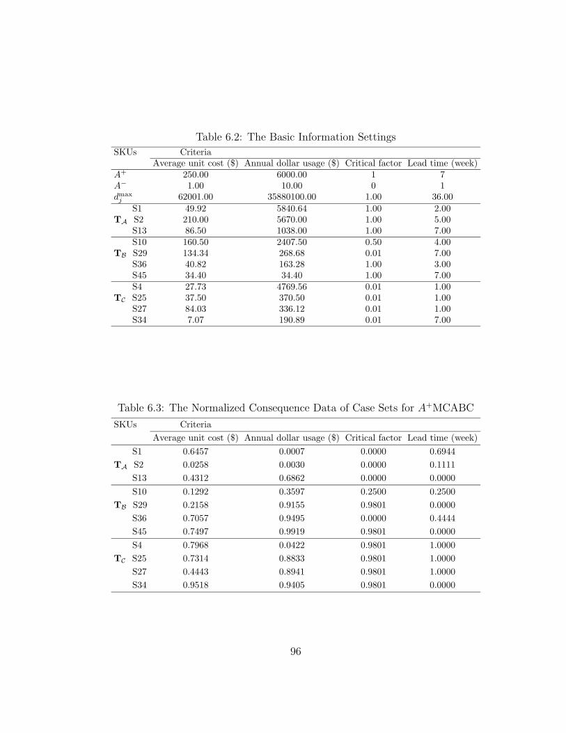
Table 6.2: The Basic Information Settings
SKUs CriteriaAverage unit cost ($) Annual dollar usage ($) Critical factor Lead time (week)
A+ 250.00 6000.00 1 7A− 1.00 10.00 0 1dmax
j 62001.00 35880100.00 1.00 36.00
S1 49.92 5840.64 1.00 2.00TA S2 210.00 5670.00 1.00 5.00
S13 86.50 1038.00 1.00 7.00S10 160.50 2407.50 0.50 4.00
TB S29 134.34 268.68 0.01 7.00S36 40.82 163.28 1.00 3.00S45 34.40 34.40 1.00 7.00S4 27.73 4769.56 0.01 1.00
TC S25 37.50 370.50 0.01 1.00S27 84.03 336.12 0.01 1.00S34 7.07 190.89 0.01 7.00
Table 6.3: The Normalized Consequence Data of Case Sets for A+MCABC
SKUs Criteria
Average unit cost ($) Annual dollar usage ($) Critical factor Lead time (week)
S1 0.6457 0.0007 0.0000 0.6944
TA S2 0.0258 0.0030 0.0000 0.1111
S13 0.4312 0.6862 0.0000 0.0000
S10 0.1292 0.3597 0.2500 0.2500
TB S29 0.2158 0.9155 0.9801 0.0000
S36 0.7057 0.9495 0.0000 0.4444
S45 0.7497 0.9919 0.9801 0.0000
S4 0.7968 0.0422 0.9801 1.0000
TC S25 0.7314 0.8833 0.9801 1.0000
S27 0.4443 0.8941 0.9801 1.0000
S34 0.9518 0.9405 0.9801 0.0000
96
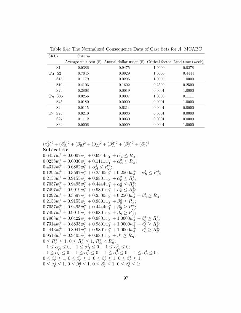
Table 6.4: The Normalized Consequence Data of Case Sets for A−MCABC
SKUs Criteria
Average unit cost ($) Annual dollar usage ($) Critical factor Lead time (week)
S1 0.0386 0.9475 1.0000 0.0278
TA S2 0.7045 0.8929 1.0000 0.4444
S13 0.1179 0.0295 1.0000 1.0000
S10 0.4103 0.1602 0.2500 0.2500
S29 0.2868 0.0019 0.0001 1.0000
TB S36 0.0256 0.0007 1.0000 0.1111
S45 0.0180 0.0000 0.0001 1.0000
S4 0.0115 0.6314 0.0001 0.0000
TC S25 0.0210 0.0036 0.0001 0.0000
S27 0.1112 0.0030 0.0001 0.0000
S34 0.0006 0.0009 0.0001 1.0000
(β2B)2 + (β3
B)2 + (β4B)2 + (β1
C)2 + (β2
C)2 + (β3
C)2 + (β4
C)2
Subject to:0.6457w+
1 + 0.0007w+2 + 0.6944w+
4 + α1A ≤ R+
A;0.0258w+
1 + 0.0030w+2 + 0.1111w+
4 + α2A ≤ R+
A;0.4312w+
1 + 0.6862w+2 + α3
A ≤ R+A;
0.1292w+1 + 0.3597w+
2 + 0.2500w+3 + 0.2500w+
4 + α1B ≤ R+
B;0.2158w+
1 + 0.9155w+2 + 0.9801w+
3 + α2B ≤ R+
B ;0.7057w+
1 + 0.9495w+2 + 0.4444w+
4 + α3B ≤ R+
B ;0.7497w+
1 + 0.9919w+2 + 0.9801w+
3 + α4B ≤ R+
B ;0.1292w+
1 + 0.3597w+2 + 0.2500w+
3 + 0.2500w+4 + β1
B ≥ R+A;
0.2158w+1 + 0.9155w+
2 + 0.9801w+3 + β2
B ≥ R+A;
0.7057w+1 + 0.9495w+
2 + 0.4444w+4 + β3
B ≥ R+A;
0.7497w+1 + 0.9919w+
2 + 0.9801w+3 + β4
B ≥ R+A;
0.7968w+1 + 0.0422w+
2 + 0.9801w+3 + 1.0000w+
4 + β1C ≥ R+
B ;0.7314w+
1 + 0.8833w+2 + 0.9801w+
3 + 1.0000w+4 + β2
C ≥ R+B ;
0.4443w+1 + 0.8941w+
2 + 0.9801w+3 + 1.0000w+
4 + β3C ≥ R+
B ;0.9518w+
1 + 0.9405w+2 + 0.9801w+
3 + β4C ≥ R+
B ;0 ≤ R+
A ≤ 1, 0 ≤ R+B ≤ 1, R+
A < R+B ;
−1 ≤ α1A ≤ 0, −1 ≤ α2
A ≤ 0, −1 ≤ α3A ≤ 0;
−1 ≤ α1B ≤ 0, −1 ≤ α2
B ≤ 0, −1 ≤ α3B ≤ 0, −1 ≤ α4
B ≤ 0;0 ≤ β1
B ≤ 1, 0 ≤ β2B ≤ 1, 0 ≤ β3
B ≤ 1, 0 ≤ β4B ≤ 1;
0 ≤ β1C ≤ 1, 0 ≤ β2
C ≤ 1, 0 ≤ β3C ≤ 1, 0 ≤ β4
C ≤ 1;
97
0.01 ≤ w+1 ≤ 0.9, 0.01 ≤ w+
2 ≤ 0.9, 0.01 ≤ w+3 ≤ 0.9, 0.01 ≤ w+
4 ≤ 0.9;w+
2 ≥ w+1 ; w+
2 ≥ w+3 ; w+
2 ≥ w+4 ;
w+1 + w+
2 + w+3 + w+
4 = 1.
Similar procedures are carried out for A−MCABC. The details are omitted, andthe results obtained are listed as: ERR = 9.9018 × 10⁻¹⁰; w− = (0.2039, 0.3138,0.2639, 0.2184); R−
C = 0.2205 and R−B = 0.4502. As ε ≪ ERR, the error is ignored.
Then, both A+ABC and A−ABC methods are applied to classify the 47 SKUs intoA, B, and C. The re-classification procedures shown in Figure 6.5 are implementedand the results are shown in Table 6.5.
98
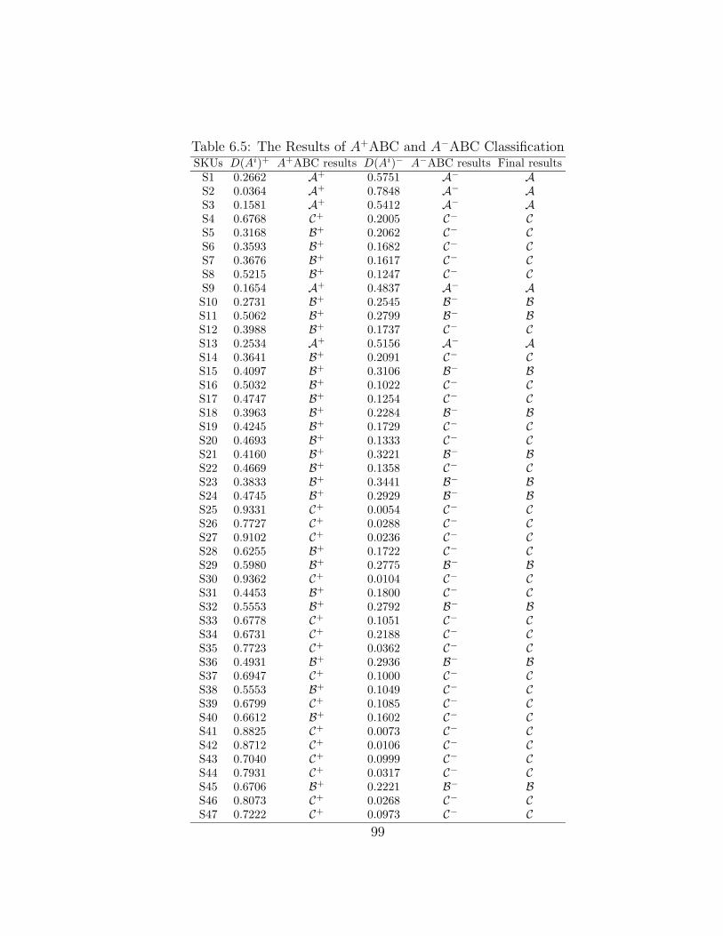
Table 6.5: The Results of A+ABC and A−ABC ClassificationSKUs D(Ai)+ A+ABC results D(Ai)− A−ABC results Final results
S1 0.2662 A+ 0.5751 A− AS2 0.0364 A+ 0.7848 A− AS3 0.1581 A+ 0.5412 A− AS4 0.6768 C+ 0.2005 C− CS5 0.3168 B+ 0.2062 C− CS6 0.3593 B+ 0.1682 C− CS7 0.3676 B+ 0.1617 C− CS8 0.5215 B+ 0.1247 C− CS9 0.1654 A+ 0.4837 A− AS10 0.2731 B+ 0.2545 B− BS11 0.5062 B+ 0.2799 B− BS12 0.3988 B+ 0.1737 C− CS13 0.2534 A+ 0.5156 A− AS14 0.3641 B+ 0.2091 C− CS15 0.4097 B+ 0.3106 B− BS16 0.5032 B+ 0.1022 C− CS17 0.4747 B+ 0.1254 C− CS18 0.3963 B+ 0.2284 B− BS19 0.4245 B+ 0.1729 C− CS20 0.4693 B+ 0.1333 C− CS21 0.4160 B+ 0.3221 B− BS22 0.4669 B+ 0.1358 C− CS23 0.3833 B+ 0.3441 B− BS24 0.4745 B+ 0.2929 B− BS25 0.9331 C+ 0.0054 C− CS26 0.7727 C+ 0.0288 C− CS27 0.9102 C+ 0.0236 C− CS28 0.6255 B+ 0.1722 C− CS29 0.5980 B+ 0.2775 B− BS30 0.9362 C+ 0.0104 C− CS31 0.4453 B+ 0.1800 C− CS32 0.5553 B+ 0.2792 B− BS33 0.6778 C+ 0.1051 C− CS34 0.6731 C+ 0.2188 C− CS35 0.7723 C+ 0.0362 C− CS36 0.4931 B+ 0.2936 B− BS37 0.6947 C+ 0.1000 C− CS38 0.5553 B+ 0.1049 C− CS39 0.6799 C+ 0.1085 C− CS40 0.6612 B+ 0.1602 C− CS41 0.8825 C+ 0.0073 C− CS42 0.8712 C+ 0.0106 C− CS43 0.7040 C+ 0.0999 C− CS44 0.7931 C+ 0.0317 C− CS45 0.6706 B+ 0.2221 B− BS46 0.8073 C+ 0.0268 C− CS47 0.7222 C+ 0.0973 C− C
99
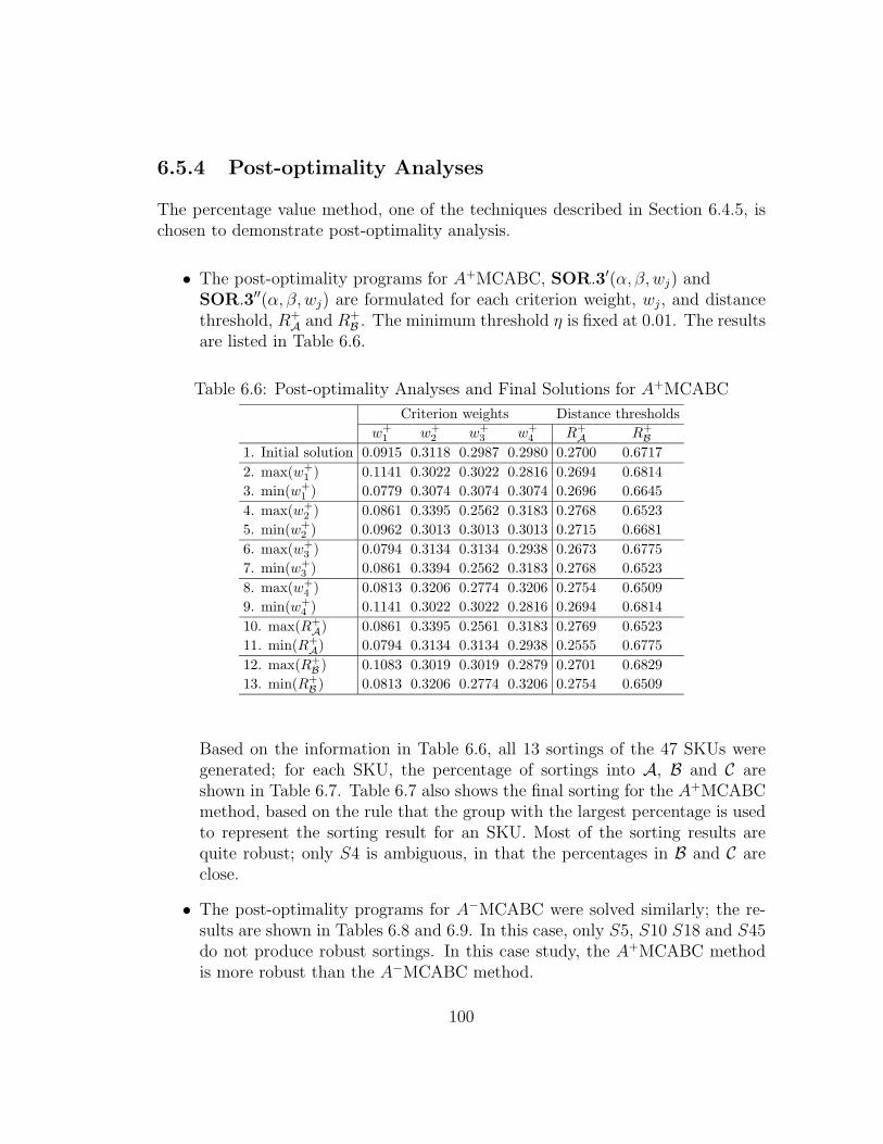
6.5.4 Post-optimality Analyses
The percentage value method, one of the techniques described in Section 6.4.5, ischosen to demonstrate post-optimality analysis.
• The post-optimality programs for A+MCABC, SOR.3′(α, β, wj) andSOR.3′′(α, β, wj) are formulated for each criterion weight, wj, and distancethreshold, R+
A and R+B . The minimum threshold η is fixed at 0.01. The results
are listed in Table 6.6.
Table 6.6: Post-optimality Analyses and Final Solutions for A+MCABC
Criterion weights Distance thresholds
w+
1 w+
2 w+
3 w+
4 R+
AR+
B
1. Initial solution 0.0915 0.3118 0.2987 0.2980 0.2700 0.6717
2. max(w+
1 ) 0.1141 0.3022 0.3022 0.2816 0.2694 0.6814
3. min(w+
1 ) 0.0779 0.3074 0.3074 0.3074 0.2696 0.6645
4. max(w+
2 ) 0.0861 0.3395 0.2562 0.3183 0.2768 0.6523
5. min(w+
2 ) 0.0962 0.3013 0.3013 0.3013 0.2715 0.6681
6. max(w+
3 ) 0.0794 0.3134 0.3134 0.2938 0.2673 0.6775
7. min(w+
3 ) 0.0861 0.3394 0.2562 0.3183 0.2768 0.6523
8. max(w+
4 ) 0.0813 0.3206 0.2774 0.3206 0.2754 0.6509
9. min(w+
4 ) 0.1141 0.3022 0.3022 0.2816 0.2694 0.6814
10. max(R+
A) 0.0861 0.3395 0.2561 0.3183 0.2769 0.6523
11. min(R+
A) 0.0794 0.3134 0.3134 0.2938 0.2555 0.6775
12. max(R+
B) 0.1083 0.3019 0.3019 0.2879 0.2701 0.6829
13. min(R+
B) 0.0813 0.3206 0.2774 0.3206 0.2754 0.6509
Based on the information in Table 6.6, all 13 sortings of the 47 SKUs weregenerated; for each SKU, the percentage of sortings into A, B and C areshown in Table 6.7. Table 6.7 also shows the final sorting for the A+MCABCmethod, based on the rule that the group with the largest percentage is usedto represent the sorting result for an SKU. Most of the sorting results arequite robust; only S4 is ambiguous, in that the percentages in B and C areclose.
• The post-optimality programs for A−MCABC were solved similarly; the re-sults are shown in Tables 6.8 and 6.9. In this case, only S5, S10 S18 and S45do not produce robust sortings. In this case study, the A+MCABC methodis more robust than the A−MCABC method.
100
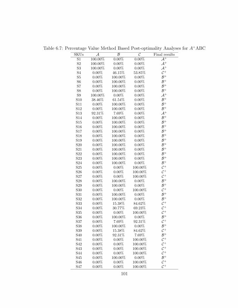
Table 6.7: Percentage Value Method Based Post-optimality Analyses for A+ABC
SKUs A B C Final resultsS1 100.00% 0.00% 0.00% A+
S2 100.00% 0.00% 0.00% A+
S3 100.00% 0.00% 0.00% A+
S4 0.00% 46.15% 53.85% C+
S5 0.00% 100.00% 0.00% B+
S6 0.00% 100.00% 0.00% B+
S7 0.00% 100.00% 0.00% B+
S8 0.00% 100.00% 0.00% B+
S9 100.00% 0.00% 0.00% A+
S10 38.46% 61.54% 0.00% B+
S11 0.00% 100.00% 0.00% B+
S12 0.00% 100.00% 0.00% B+
S13 92.31% 7.69% 0.00% A+
S14 0.00% 100.00% 0.00% B+
S15 0.00% 100.00% 0.00% B+
S16 0.00% 100.00% 0.00% B+
S17 0.00% 100.00% 0.00% B+
S18 0.00% 100.00% 0.00% B+
S19 0.00% 100.00% 0.00% B+
S20 0.00% 100.00% 0.00% B+
S21 0.00% 100.00% 0.00% B+
S22 0.00% 100.00% 0.00% B+
S23 0.00% 100.00% 0.00% B+
S24 0.00% 100.00% 0.00% B+
S25 0.00% 0.00% 100.00% C+
S26 0.00% 0.00% 100.00% C+
S27 0.00% 0.00% 100.00% C+
S28 0.00% 100.00% 0.00% B+
S29 0.00% 100.00% 0.00% B+
S30 0.00% 0.00% 100.00% C+
S31 0.00% 100.00% 0.00% B+
S32 0.00% 100.00% 0.00% B+
S33 0.00% 15.38% 84.62% C+
S34 0.00% 30.77% 69.23% C+
S35 0.00% 0.00% 100.00% C+
S36 0.00% 100.00% 0.00% B+
S37 0.00% 7.69% 92.31% C+
S38 0.00% 100.00% 0.00% B+
S39 0.00% 15.38% 84.62% C+
S40 0.00% 92.31% 7.69% B+
S41 0.00% 0.00% 100.00% C+
S42 0.00% 0.00% 100.00% C+
S43 0.00% 0.00% 100.00% C+
S44 0.00% 0.00% 100.00% C+
S45 0.00% 100.00% 0.00% B+
S46 0.00% 0.00% 100.00% C+
S47 0.00% 0.00% 100.00% C+
101
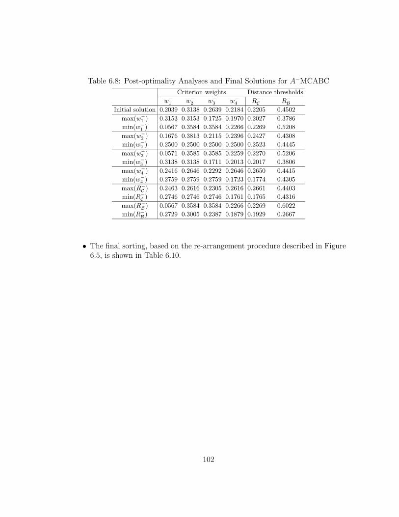
Table 6.8: Post-optimality Analyses and Final Solutions for A−MCABC
Criterion weights Distance thresholds
w−
1 w−
2 w−
3 w−
4 R−
CR−
B
Initial solution 0.2039 0.3138 0.2639 0.2184 0.2205 0.4502
max(w−
1 ) 0.3153 0.3153 0.1725 0.1970 0.2027 0.3786
min(w−
1 ) 0.0567 0.3584 0.3584 0.2266 0.2269 0.5208
max(w−
2 ) 0.1676 0.3813 0.2115 0.2396 0.2427 0.4308
min(w−
2 ) 0.2500 0.2500 0.2500 0.2500 0.2523 0.4445
max(w−
3 ) 0.0571 0.3585 0.3585 0.2259 0.2270 0.5206
min(w−
3 ) 0.3138 0.3138 0.1711 0.2013 0.2017 0.3806
max(w−
4 ) 0.2416 0.2646 0.2292 0.2646 0.2650 0.4415
min(w−
4 ) 0.2759 0.2759 0.2759 0.1723 0.1774 0.4305
max(R−
C) 0.2463 0.2616 0.2305 0.2616 0.2661 0.4403
min(R−
C) 0.2746 0.2746 0.2746 0.1761 0.1765 0.4316
max(R−
B) 0.0567 0.3584 0.3584 0.2266 0.2269 0.6022
min(R−
B) 0.2729 0.3005 0.2387 0.1879 0.1929 0.2667
• The final sorting, based on the re-arrangement procedure described in Figure6.5, is shown in Table 6.10.
102

Table 6.9: Percentage Value Method Based Post-optimality Analyses for A−ABC
SKUs A B C Final resultsS1 100.00% 0.00% 0.00% A−
S2 100.00% 0.00% 0.00% A−
S3 100.00% 0.00% 0.00% A−
S4 0.00% 7.69% 92.31% C−
S5 0.00% 53.85% 46.15% B−
S6 0.00% 0.00% 100.00% C−
S7 0.00% 0.00% 100.00% C−
S8 0.00% 0.00% 100.00% C−
S9 84.62% 15.38% 0.00% A−
S10 0.00% 53.85% 46.15% B−
S11 0.00% 61.54% 38.46% B−
S12 0.00% 0.00% 100.00% C−
S13 100.00% 0.00% 0.00% A−
S14 0.00% 30.77% 69.23% C−
S15 7.69% 92.31% 0.00% B−
S16 0.00% 0.00% 100.00% C−
S17 0.00% 0.00% 100.00% C−
S18 0.00% 53.85% 46.15% B−
S19 0.00% 0.00% 100.00% C−
S20 0.00% 0.00% 100.00% C−
S21 7.69% 92.31% 0.00% B−
S22 0.00% 0.00% 100.00% C−
S23 7.69% 92.31% 0.00% B−
S24 0.00% 69.23% 30.77% B−
S25 0.00% 0.00% 100.00% C−
S26 0.00% 0.00% 100.00% C−
S27 0.00% 0.00% 100.00% C−
S28 0.00% 0.00% 100.00% C−
S29 0.00% 100.00% 0.00% B−
S30 0.00% 0.00% 100.00% C−
S31 0.00% 0.00% 100.00% C−
S32 0.00% 61.54% 38.46% B+
S33 0.00% 0.00% 100.00% C−
S34 0.00% 0.00% 100.00% C−
S35 0.00% 0.00% 100.00% C−
S36 0.00% 61.54% 38.46% B−
S37 0.00% 0.00% 100.00% C−
S38 0.00% 0.00% 100.00% C−
S39 0.00% 0.00% 100.00% C−
S40 0.00% 0.00% 100.00% C−
S41 0.00% 0.00% 100.00% C−
S42 0.00% 0.00% 100.00% C−
S43 0.00% 0.00% 100.00% C−
S44 0.00% 0.00% 100.00% C−
S45 0.00% 53.85% 46.15% B−
S46 0.00% 0.00% 100.00% C−
S47 0.00% 0.00% 100.00% C−
103
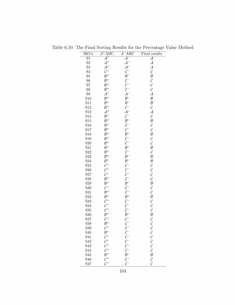
Table 6.10: The Final Sorting Results for the Percentage Value Method
SKUs A+ABC A−ABC Final resultsS1 A+ A− AS2 A+ A− AS3 A+ A− AS4 C+ C− CS5 B+ B− BS6 B+ C− CS7 B+ C− CS8 B+ C− CS9 A+ A− AS10 B+ B− BS11 B+ B− BS12 B+ C− CS13 A+ A− AS14 B+ C− CS15 B+ B− BS16 B+ C− CS17 B+ C− CS18 B+ B− BS19 B+ C− CS20 B+ C− CS21 B+ B− BS22 B+ C− CS23 B+ B− BS24 B+ B− BS25 C+ C− CS26 C+ C− CS27 C+ C− CS28 B+ C− CS29 B+ B− BS30 C+ C− CS31 B+ C− CS32 B+ B+ BS33 C+ C− CS34 C+ C− CS35 C+ C− CS36 B+ B− BS37 C+ C− CS38 B+ C− CS39 C+ C− CS40 B+ C− CS41 C+ C− CS42 C+ C− CS43 C+ C− CS44 C+ C− CS45 B+ B− BS46 C+ C− CS47 C+ C− C
104
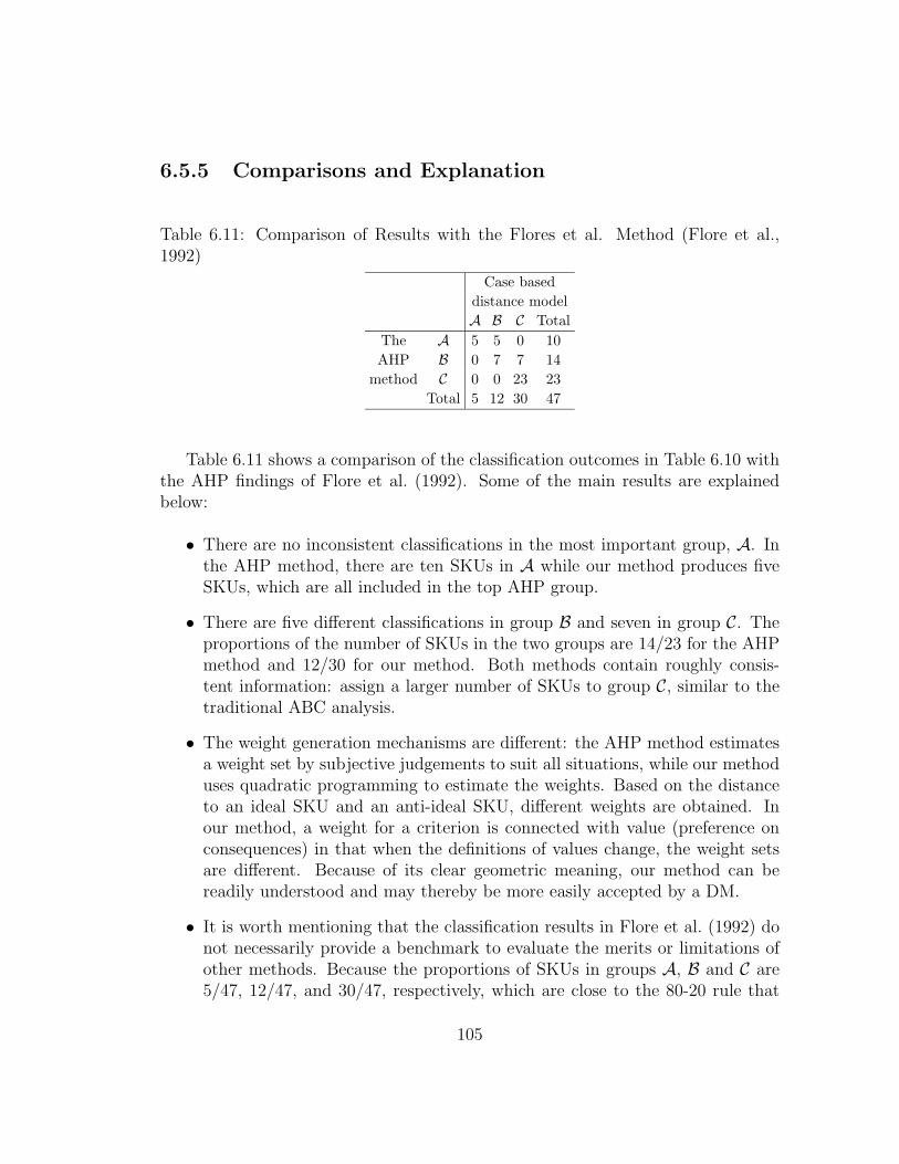
6.5.5 Comparisons and Explanation
Table 6.11: Comparison of Results with the Flores et al. Method (Flore et al.,1992)
Case based
distance model
A B C Total
The A 5 5 0 10
AHP B 0 7 7 14
method C 0 0 23 23
Total 5 12 30 47
Table 6.11 shows a comparison of the classification outcomes in Table 6.10 withthe AHP findings of Flore et al. (1992). Some of the main results are explainedbelow:
• There are no inconsistent classifications in the most important group, A. Inthe AHP method, there are ten SKUs in A while our method produces fiveSKUs, which are all included in the top AHP group.
• There are five different classifications in group B and seven in group C. Theproportions of the number of SKUs in the two groups are 14/23 for the AHPmethod and 12/30 for our method. Both methods contain roughly consis-tent information: assign a larger number of SKUs to group C, similar to thetraditional ABC analysis.
• The weight generation mechanisms are different: the AHP method estimatesa weight set by subjective judgements to suit all situations, while our methoduses quadratic programming to estimate the weights. Based on the distanceto an ideal SKU and an anti-ideal SKU, different weights are obtained. Inour method, a weight for a criterion is connected with value (preference onconsequences) in that when the definitions of values change, the weight setsare different. Because of its clear geometric meaning, our method can bereadily understood and may thereby be more easily accepted by a DM.
• It is worth mentioning that the classification results in Flore et al. (1992) donot necessarily provide a benchmark to evaluate the merits or limitations ofother methods. Because the proportions of SKUs in groups A, B and C are5/47, 12/47, and 30/47, respectively, which are close to the 80-20 rule that
105
is observed in many practical inventory systems, our model provides a soundclassification result.
6.6 Conclusions
The classical ABC analysis is a straightforward approach that assists a DM inachieving cost-effective inventory management by arranging SKUs according totheir annual dollar usages. However, in many situations, the DM should considerother criteria, such as lead time and criticality, in addition to annual dollar usage.MCABC procedures furnish an inventory manager with additional flexibility toaccount for more factors in classifying SKUs. This chapter proposes a case-baseddistance model to handle MCABC problems under the umbrella of MCDA theory.A case study is developed to illustrate how the procedure can be applied; the resultsdemonstrate that this approach is robust and can produce sound classifications ofSKUs when multiple criteria are to be considered.
106
Chapter 7
Sorting Problem Extension inNegotiation
7.1 Introduction
A case-based distance model founded on multiple criteria decision analysis theoryis proposed for bilateral negotiations (BN) involving multiple issues. The uniquefeature of this negotiation model is that weighted Euclidean distance is employed torepresent the negotiators’ preferences; a case-based distance algorithm then helpsnegotiators express their preferences over different offers (alternatives) and suggestshow to find better outcomes. The procedure takes advantage of the easily under-stood geometric meaning of Euclidean distance. The remainder of this chapter isorganized as follows. Section 2 provides a brief literature review of group negoti-ation and decision. Next, Section 3 gives a basic background of multiple criteriadecision analysis and defines a BN problem. Section 4 proposes a case-based dis-tance model to solve this problem, while Section 5 presents a case study of BNin a business context. Finally, some conclusions are presented in Section 6. Thecontributions of this chapter are based upon research by Chen et al. (Chen et al.,2005f).
7.2 Motivation
Negotiation is an important research topic in many disciplines including social sci-ences, economics, game theory, decision support systems, engineering, and multi-
107
agent theory. In practice, people negotiate on a very broad range of subjects in-cluding diplomatic issues, international conflicts, meeting schedules, productionplans and purchases. Within the few last decades, many methodologies have beenproposed to study negotiations. Some of them are summarized next.
Pruitt (1981) studies negotiations from the point of view of social psychology,emphasizing cognitive processes. Many explanations are given for the motives, per-ceptions, and other micro-processes driving a negotiator’s behavior, supported byevidence from laboratory experiments. Raiffa’s influential book (Raiffa et al., 2002)divides negotiations into several classes according to the number of negotiators andthe number of issues involved: two negotiators with one issue, two negotiatorswith many issues, or many negotiators with many issues. Here we address a two-negotiator multi-issue problem. Game theory provides a mathematical study ofrational behavior in conflicts: models of negotiation address whether an agreementcan be reached and how protocols that achieve Pareto optimal solutions should bedesigned (Brams, 2003). For example, based on multiple attribute utility theory,Ehtamo et al. (1999) design an interactive method to assist negotiators in mov-ing from an initial inefficient point to an efficient solution. This method may beapplicable to negotiations on political issues. Some approaches in multiple criteriadecision analysis (MCDA) address group decision making and negotiations. For ex-ample, using distance minimization (related to goral programming), Kersten (1985)developed NEGO, a group decision support system, and Kersten and Szapiro (1986)introduced a general approach for structuring and modelling negotiations based ona concept of pressure.
Recently, with the development of internet-based electronic businesses, muchresearch has focused on the application of computers and the internet to sup-port or even automate negotiation processes (Kersten, 2004). New computingand communication technologies have introduced new opportunities for the de-sign and deployment of software capable of supporting negotiations. Negotiationsconducted over the web are commonly called e-negotiations, have an importantrole in e-marketplaces especially in personalizing and customizing processes. Afew implementations of e-negotiation systems are available on the internet; forexample, the special purpose system, Inspire, has been in operation since 1996(http://interneg.org/inspire) (Kersten, 2004).
Most current e-negotiation systems employ simple additive value (utility) func-tions to evaluate the preferences of negotiators. But in practice many factors influ-ence the effectiveness of human negotiations. Vetschera (2004) checked the analysisof about 4,700 multi-attribute utility functions elicited by Inspire systems and re-ported that negotiators’ behavior during the negotiation process contradicted their
108
imputed preferences in about 25% of all cases. He concluded that a simple additiveutility function is probably not an adequate method to evaluate the performanceof negotiators in such negotiations.
7.3 Multiple Issue Bilateral Negotiations
The bilateral negotiation model presented in this thesis is described in detail asfollows:
(1) There are two DMs, DM1 and DM2, who are jointly making a decision(negotiation) in a decision problem with multiple criteria (issues), Q = {1, 2, ..., q},such as price, quantity and delivery time.
(2) Consequences on every criterion j ∈ Q are unambiguously measurable.Moreover, on each criterion j ∈ Q, an indifference threshold εj is agreed upon byDM1 and DM2 (Vincke, 1992), such that differences in values of cj(A) less than εj
are not meaningful and can be ignored. For example, differences in delivery timeless than one day may not be meaningful because of the production cycle or, in thepurchase of a car, people might bargain over prices in $ 10 intervals (while, in thepurchase of a television, their threshold might equal $ 1).
(3) The maximum consequence on criterion j is cmaxj ∈ R+ and the minimum
consequence is cminj ∈ R+, where cmax
j and cminj are known to both DM1 and DM2,
and cmaxj > cmin
j . The interval [cminj , cmax
j ] is the consequence interval for criterionj. For example, for the criterion of price, cmax
j and cminj might be a ceiling and floor
that are determined external to the negotiation. We assume that 1εj
(cmaxj − cmin
j ) is
a positive integer for each criterion j ∈ Q.
It follows from (3) that, for each criterion j, j = 1, 2, ..., q, the number of possibleconsequence values is nj = 1 + 1
εj(cmax
j − cminj ). In fact, the consequence values on
criterion j (in increasing order) are cminj < cmin
j +εj < ... < cminj +(nj −2)εj < cmax
j .Thus, the number of feasible alternatives for the BN problem is |A| = n = n1 · n2 ·... · nq.
109
7.4 A Case-based Distance Model for Bilateral
Negotiation
7.4.1 Case Set Assumptions
To assist DMs in providing a case set, we assume that a set of ordinally definedlinguistic grades, such as {excellent, very good, good, fair, bad} can be used toassess alternatives. The linguistic grade set is denoted as L = {1, 2, ..., g, ..., L},where 1 is the best grade and L is the worst grade. For A,B ∈ A, we say thatA ∼k B (DMk equally prefers A and B) whenever A and B are assigned the samelinguistic grade by DMk, and that A ≻k B (DMk prefers A to B) whenever A isassigned a higher linguistic grade than B by DMk.
Within the alternative set A, suppose that DMk (k = 1, 2) specifies a repre-sentative case set Zk = {Z1
k , Z2k , ..., Z
rk , ..., Z
mk } ⊂ A, in which each alternative is
assigned a linguistic grade. Let mk denote the number of alternatives in Zk. Sup-pose that Gk : Zk → L is DMk’s assignment of grades, so that Gk(Z
rk) = gr
k ∈ L isthe grade assigned by DMk to Zr
k . Furthermore, assume that at least one case isassigned to the best grade, so that |{Zr
k : grk = 1}| = m1
k ≥ 1, for k = 1, 2. Assumefurther (without loss of generality) that r < s implies Gk(Z
rk) ≤ Gk(Z
sk), i.e. that
Zk is listed in decreasing order of linguistic grade.
Our idea, from case-based reasoning, is that Zk should enable us to estimatecriterion weights for DMk, which would simplify the process of acquisition of preciseweights, enabling DMk to express his or her preferences more easily. WeightedEuclidean distance is employed since it has a clear geometric meaning, which canbe easily understood and accepted by a DM to represent his or her aggregatedpreference. The details are explained next.
7.4.2 Distance Assumptions
Given the representative case set Zk, Zk, the centroid of Zk is deemed to be afictitious alternative at the center of all cases assigned to the best grade. Thus,
cj
(
Zk
)
=1
m1k
m1k
∑
r=1
cj
(
Zrk
)
, (7.1)
For each j = 1, 2, ..., q, define dmaxj = max
r=1,2,...,mk
(
cj(Zrk) − cj(Zk)
)2; then dmax
j is
the normalization factor for criterion j. For DMk (k = 1, 2) the distance between
110
Ai ∈ A and Zk on criterion j is
dj(Ai, Zk) = dk
j (Ai) =
(
cj(Ai) − cj(Zk)
)2
dmaxj
. (7.2)
In particular, if Ai = Zrk , then (7.2) defines dk
j (Zrk). For DMk (k = 1, 2) the
distance between alternatives Ai and Zk is then
Dk(Ai) = Dk(A
i, Zk) =
{
∑
j∈Q
wkj · dk
j (Ai)
}1/2
, (7.3)
where wk = (wk1 , w
k2 , ..., w
kq ) is a weight vector for DMk (later we will determine an
appropriate weight vector for DMk). Note that (7.3) defines Dk(Zrk) if Ai = Zr
k . Itis easy to verify that 0 ≤ Dk(A
i) ≤ 1 for k = 1, 2. Thus, the distances from Zk toall alternatives are normalized for easy comparison.
In terms of the aggregation approach to MCDA discussed above, dkj (A
i) is anal-ogous to vi
j in (2.1), and Dk(Ai) is analogous to V (Ai) in (2.5) for DMk. It is
assumed that Zk is a good estimate of the ideal alternative (the most preferred al-ternative) so that the closer Ai to Zk, the greater DMk’s preference; in other words,smaller values of Dk(A
i) indicate greater preference. The distance of an alternativeis thus defined to be the distance between the alternative and the centroid of thecase set.
A similar idea has been used in cluster analysis: cluster membership of a datumis determined by evaluation of a pre-defined distance between this datum and thecluster centroid. If the DM can explicitly specify the ideal alternative, Z∗, thenZ∗ could be used instead of the centroid to measure the distances. Yet anotherapproach is to define the centroid of Zk to be the center of the cases assigned tothe worst grade, so that DMk’s preference increases with distance from Zk.
7.4.3 Distance Intervals for Linguistic Grades
Based on the distance definitions above and assuming a specific weight vector, adistance interval can be assigned to Zr
k ∈ Zk based on its linguistic grade as assessedby DMk. For example, if Zr
k is evaluated as belonging to the highest grade, i.e.Gk(Z
rk) = 1, then Dk(Z
rk) ∈ [0, 1
L]. More generally, if the linguistic grade for Zr
k
is grk, then Dk(Z
rk) ∈ [
grk−1
L,
grk
L] for r = 1, 2, ...,mk. Note that the gaps between
adjacent linguistic grades are represented by equal spacing. We believe this setting
111

is easily understood by a DM. Of course, a DM can adjust it to fit in with his andher instinctive preference; for example, the ordinal preference expressions discussedin Cook and Kress (1991) could be employed for this purpose.
7.4.4 Weight Determination and Distance Construction
For j ∈ Q, the weight wkj presents DMk’s relative importance for criterion j
compared with other criteria in the criteria set Q. Here we try to obtain wk =(wk
1 , wk2 , ..., w
kq ) by a case-based reasoning model based on the information Zk pro-
vided by DMk. The details are explained below.
Assuming that Zrk ∈ Zk is assigned the linguistic grade Gk(Z
∗k) = gr
k, the dis-
tance from Zk to Zrk , Dk(Z
rk), must satisfy Dk(Z
rk) ∈ [
grk−1
L,
grk
L], provided there are
no inconsistent judgements. So the following constraints are associated with Zrk :
Dk(Zrk) + αr
k ≤ grk
L; (7.4)
Dk(Zrk) + βr
k ≥ grk − 1
L. (7.5)
where −1 ≤ αrk ≤ 0 is an upper error bound for the DM’s inconsistent judgements
when Dk(Zrk) >
grk
Land 0 ≤ βr
k ≤ 1 is a lower error bound for the DM’s inconsistent
judgements when Dk(Zrk) <
grk−1
L. Clearly, (7.4) and (7.5) are equivalent to
{
∑
j∈Q
wkj d
kj (Z
rk)
}1/2
+ αrk ≤ gr
k
L; (7.6)
{
∑
j∈Q
wkj d
kj (Z
rk)
}1/2
+ βrk ≥ gr
k − 1
L. (7.7)
Similarly, upper and lower error bounds exist for all alternatives in Zk, so that the
overall error in Zk can be measured as ERRk =mk∑
r=1
[
(−αrk) + (βr
k)]
.
Figure 7.1 shows the relationships between Zrk and Zk when there are two criteria
(dimensions). The same settings are used in Figures 7.3 to 7.8. Note that in Figure7.1, L = 4 and Zr
k is assessed at the 3rd linguistic grade (Gk(Zrk) = 3). Taking Zk as
the center, three concentric ellipses (depending on the weight vector, they must beconcentric circles) partition the alternative set A into four parts representing the
112
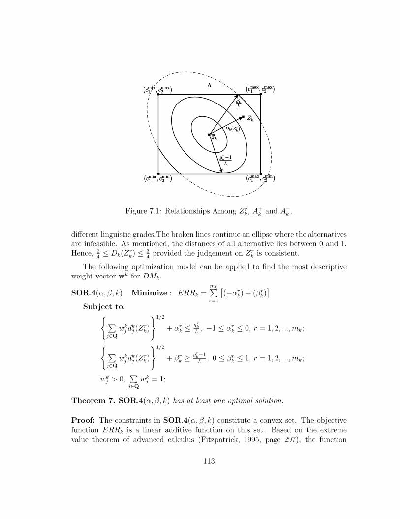
A
.
.
(cmin1, cmin2)(cmin
1, cmin2)
(cmin1, cmax2
)(cmin1, cmax2
).
(cmax1
, cmax2
)(cmax1
, cmax2
)
(cmax1
, cmin2)(cmax
1, cmin2)
.
.
ZkZk
. ZrkZrk
Dk(Zrk)Dk(Zrk)
grk
1
L
grk
1
L
grk
L
grk
L
Figure 7.1: Relationships Among Zrk , A+
k and A−k .
different linguistic grades.The broken lines continue an ellipse where the alternativesare infeasible. As mentioned, the distances of all alternative lies between 0 and 1.Hence, 2
4≤ Dk(Z
rk) ≤ 3
4provided the judgement on Zr
k is consistent.
The following optimization model can be applied to find the most descriptiveweight vector wk for DMk.
SOR.4(α, β, k) Minimize : ERRk =mk∑
r=1
[
(−αrk) + (βr
k)]
Subject to:{
∑
j∈Q
wkj d
kj (Z
rk)
}1/2
+ αrk ≤ gr
k
L, −1 ≤ αr
k ≤ 0, r = 1, 2, ...,mk;
{
∑
j∈Q
wkj d
kj (Z
rk)
}1/2
+ βrk ≥ gr
k−1
L, 0 ≤ βr
k ≤ 1, r = 1, 2, ...,mk;
wkj > 0,
∑
j∈Q
wkj = 1;
Theorem 7. SOR.4(α, β, k) has at least one optimal solution.
Proof: The constraints in SOR.4(α, β, k) constitute a convex set. The objectivefunction ERRk is a linear additive function on this set. Based on the extremevalue theorem of advanced calculus (Fitzpatrick, 1995, page 297), the function
113
ERR is continuous and the set of all possible variables is bounded, ERR attainsits minimum at least once. ¤
An indifference distance threshold, ε should be set to evaluate the error, ERRk,generated by D(α, β, k): When ERRk ≤ ε, the error is small and can be ignored, sothe information in the case set Zk provided by DMk is considered to be consistent;when ERRk > ε, the error cannot be ignored and there is some inconsistency in Zk.If so, DMk should reconsider the case set Zk and the linguistic grades assigned toit. Recall that εj is the indifference threshold on criterion j ∈ Q, which suggests anoverall indifference measure of
∑
j∈Q
1dmax
j(εj). However, a typical indifference distance
threshold is 110n
, where n is the number of alternatives in A. Therefore, a goodstandard for the indifference distance threshold is ε = min{
∑
j∈Q
110dmax
j(εj),
110n
}.
Similar to the discussion in Section 6.4.3, a DM may wish to provide informationto make the results reflect more accurately his or her intrinsic preferences, whichmay be approximate, about weights for incorporation into SOR.4(α, β, k). Theimprecise preference expressions proposed by Sage and White (1984), and Eum etal. (2001) fulfill this purpose. Some imprecise weight preference expressions arelisted below:
• Weak ranking:w1 ≥ w2 ≥ · · · ≥ wq > 0; (7.8)
• Strict ranking:wj − wj+1 ≥ ǫj, j ∈ Q, (7.9)
where ǫj is a small positive value;
• Difference ranking:
w1 − w2 ≥ · · · ≥ wq−1 − wq ≥ 0; (7.10)
• Fixed bounds:Lj ≤ wj ≤ Uj, j ∈ Q, (7.11)
where Lj and Uj are lower and upper bounds for wj, respectively;
Obviously, when any of these constraints is incorporated into SOR.4(α, β, k),the program still has at least one optimal solution.
114
7.4.5 Post-optimality Analyses
Because SOR.4(α, β, k) may have multiple optimal solutions for criterion weights,it is necessary to examine the robustness of the optimal solution via post-optimalityanalyses. There are several ways to handle the existence of multiple or near optimalsolutions of SOR.4(α, β, k):
• Assuming the optimal objective value of SOR.4(α, β, k) is ERR∗, a post-optimal analysis of wj can be carried out based on the suggestions of Jacquet-Lagreze and Siskos (1982) through the following programs:
SOR.4′(α, β, k, wj) Maximize : wj
Subject to:
ERR ≤ max{η, (1 + η)ERR∗},all the constraints of SOR.4(α, β, k),constraints (7.8) - (7.11) as applicable.
where η is a positive number.
SOR.4′′(α, β, k, wj) Minimize : wj
Subject to:
ERR ≤ max{η, (1 + η)ERR∗},all the constraints of SOR.4(α, β, k),constraints (7.8) - (7.11) as applicable.
Similar post-optimality analyses can be carried out for each j ∈ Q. Then theaverage weight for each criterion from the procedures may be considered asthe final result This procedure is adapted from the suggestions of Jacquet-Lagreze and Siskos (1982).
• Another way to conduct post-optimality analysis is to employ different opti-mization software packages, such as LINGO or Matlab, or to carry out theoptimization algorithms with different initializations to identify multiple op-timal solutions, if any. When SOR.4(α, β, k) has multiple solutions, the DMcan select a solution which is in some way “closest” to his or her intuition —for example, most consistent with any imprecise weight information given in(7.8) - (7.11).
115
7.4.6 Distance-based Bilateral Negotiation Support System
Based on the distance representation of preference developed above, a distance-based negotiation support system is proposed to solve BN problems. It involvesthree phases as shown in Figure 7.2: pre-negotiation, negotiation and adjustment.In the pre-negotiation phase, the BN problem is constructed and parameters areset as in Section 2.2. Then using the linguistic grade vector L, each DM selects acase set Zk ∈ A (k = 1, 2) and assigns linguistic grades. During the negotiationphase the system provides some suggested alternatives based on available preferenceinformation from both sides. With the assistance of computer techniques, the DMscan easily evaluate different alternatives based upon their distances, especially intwo-criterion consequence space. Interactive decision maps, developed by Lotovet al. (2004) for MCDA, could be employed to carry out this procedure. Sinceeach DM’s preferences can be represented geometrically, the DMs can evaluatealternatives (offers) and carry out negotiations.
The adjustment phase is used if the DMs appear to achieve an inefficient com-promise; the system presents some efficient alternatives and invites the DMs tocontinue the negotiation until an efficient compromise alternative is reached.
The detailed procedure follows:
(1) Construct the negotiation problem: DM1 and DM2 must determine unambigu-ously the issue (criterion) set Q on which they are negotiating.
(2) Set the initial negotiation parameters. First DM1 and DM2 must select cmaxj ,
cminj and εj for each criterion j ∈ Q. Based on these settings, the alternative set,
A, can be identified and presented to DM1 and DM2. Then a set of linguisticgrades, L, to enable DMs to assess case sets, must be prepared.
(3) Acquire a case set Zk from DMk for k = 1, 2 with settings given by Gk : Zk → L.Note that it is required that at least one case is assigned to the top grade.
(4) Compute Zk and dkj (Z
rk) for r = 1, 2, ...,mk and k = 1, 2 using (7.1) and (7.2).
Then for each k, apply SOR.4(α, β, k) to generate the weight vector wk andpresent it to DMk privately. Check the error ERRk. If ERRk > ε, ask DMk
to repeat step (3); if ERRk ≤ ε, continue. Post-optimality analyses can alsobe carried out to confirm the robustness of the results.
(5) Generate a suggested alternative set T ⊂ A and present it to DM1 and DM2
publicly. Initially, T is constructed as described in Section 7.4.7 using equal val-ues of the acceptable distance thresholds (explained later) for both DMs. Then,
116
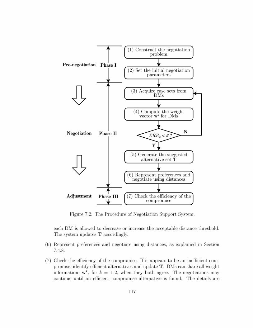
Phase II
Phase III
Phase IPre-negotiation
Negotiation
Adjustment
(1) Construct the negotiation problem
(2) Set the initial negotiation parameters
(3) Acquire case sets from DMs
(4) Compute the weight vector wk for DMs
(5) Generate the suggested alternative set T
Y
N
(6) Represent preferences and negotiate using distances
ERRk < ?
(7) Check the efficiency of the compromise
Figure 7.2: The Procedure of Negotiation Support System.
each DM is allowed to decrease or increase the acceptable distance threshold.The system updates T accordingly.
(6) Represent preferences and negotiate using distances, as explained in Section7.4.8.
(7) Check the efficiency of the compromise. If it appears to be an inefficient com-promise, identify efficient alternatives and update T. DMs can share all weightinformation, wk, for k = 1, 2, when they both agree. The negotiations maycontinue until an efficient compromise alternative is found. The details are
117
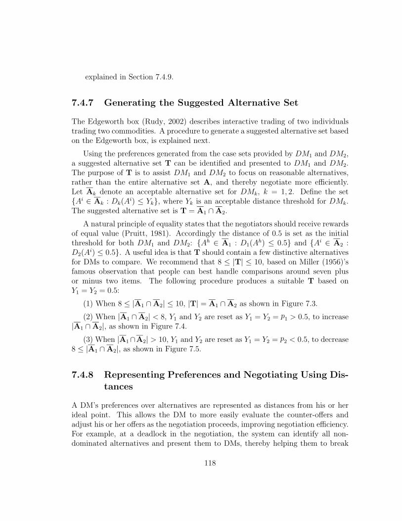
explained in Section 7.4.9.
7.4.7 Generating the Suggested Alternative Set
The Edgeworth box (Rudy, 2002) describes interactive trading of two individualstrading two commodities. A procedure to generate a suggested alternative set basedon the Edgeworth box, is explained next.
Using the preferences generated from the case sets provided by DM1 and DM2,a suggested alternative set T can be identified and presented to DM1 and DM2.The purpose of T is to assist DM1 and DM2 to focus on reasonable alternatives,rather than the entire alternative set A, and thereby negotiate more efficiently.Let Ak denote an acceptable alternative set for DMk, k = 1, 2. Define the set{Ai ∈ Ak : Dk(A
i) ≤ Yk}, where Yk is an acceptable distance threshold for DMk.The suggested alternative set is T = A1 ∩ A2.
A natural principle of equality states that the negotiators should receive rewardsof equal value (Pruitt, 1981). Accordingly the distance of 0.5 is set as the initialthreshold for both DM1 and DM2: {Ah ∈ A1 : D1(A
h) ≤ 0.5} and {Ai ∈ A2 :D2(A
i) ≤ 0.5}. A useful idea is that T should contain a few distinctive alternativesfor DMs to compare. We recommend that 8 ≤ |T| ≤ 10, based on Miller (1956)’sfamous observation that people can best handle comparisons around seven plusor minus two items. The following procedure produces a suitable T based onY1 = Y2 = 0.5:
(1) When 8 ≤ |A1 ∩ A2| ≤ 10, |T| = A1 ∩ A2 as shown in Figure 7.3.
(2) When |A1 ∩A2| < 8, Y1 and Y2 are reset as Y1 = Y2 = p1 > 0.5, to increase|A1 ∩ A2|, as shown in Figure 7.4.
(3) When |A1∩A2| > 10, Y1 and Y2 are reset as Y1 = Y2 = p2 < 0.5, to decrease8 ≤ |A1 ∩ A2|, as shown in Figure 7.5.
7.4.8 Representing Preferences and Negotiating Using Dis-tances
A DM’s preferences over alternatives are represented as distances from his or herideal point. This allows the DM to more easily evaluate the counter-offers andadjust his or her offers as the negotiation proceeds, improving negotiation efficiency.For example, at a deadlock in the negotiation, the system can identify all non-dominated alternatives and present them to DMs, thereby helping them to break
118
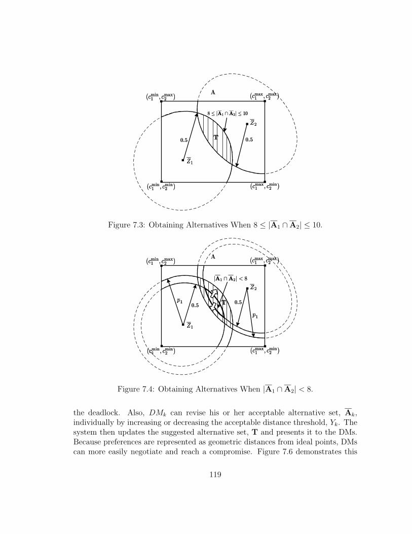
A
.
.
(cmin1, cmin2)(cmin
1, cmin2)
(cmin1, cmax2
)(cmin1, cmax2
).
(cmax1
, cmax2
)(cmax1
, cmax2
)
(cmax1
, cmin2)(cmax
1, cmin2)
.
.
.
Z1Z1
Z2Z2
0.5 0.5
8 |A1 A2| 108 |A1 A2| 10
TT
Figure 7.3: Obtaining Alternatives When 8 ≤ |A1 ∩ A2| ≤ 10.
A
.
.
(cmin1, cmin2)(cmin
1, cmin2)
(cmin1, cmax2
)(cmin1, cmax2
).
(cmax1
, cmax2
)(cmax1
, cmax2
)
(cmax1
, cmin2)(cmax
1, cmin2)
.
.
.
Z1Z1
Z2Z2
0.50.5TT
|A1 A2| < 8|A1 A2| < 8
p1p1
p1p1
Figure 7.4: Obtaining Alternatives When |A1 ∩ A2| < 8.
the deadlock. Also, DMk can revise his or her acceptable alternative set, Ak,individually by increasing or decreasing the acceptable distance threshold, Yk. Thesystem then updates the suggested alternative set, T and presents it to the DMs.Because preferences are represented as geometric distances from ideal points, DMscan more easily negotiate and reach a compromise. Figure 7.6 demonstrates this
119
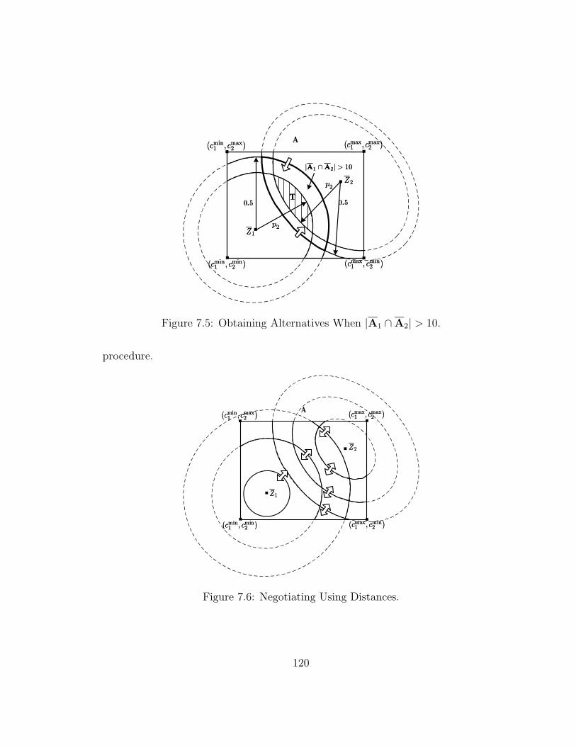
A
.
.
(cmin1, cmin2)(cmin
1, cmin2)
(cmin1, cmax2
)(cmin1, cmax2
).
(cmax1
, cmax2
)(cmax1
, cmax2
)
(cmax1
, cmin2)(cmax
1, cmin2)
.
.
.
Z1Z1
Z2Z2
0.5 0.5TT
|A1 A2| > 10|A1 A2| > 10
p2p2
p2p2
Figure 7.5: Obtaining Alternatives When |A1 ∩ A2| > 10.
procedure.
A
.
.
(cmin1, cmin2)(cmin
1, cmin2)
(cmin1, cmax2
)(cmin1, cmax2
).
(cmax1
, cmax2
)(cmax1
, cmax2
)
(cmax1
, cmin2)(cmax
1, cmin2)
.
.
.
Z1Z1
Z2Z2
Figure 7.6: Negotiating Using Distances.
120
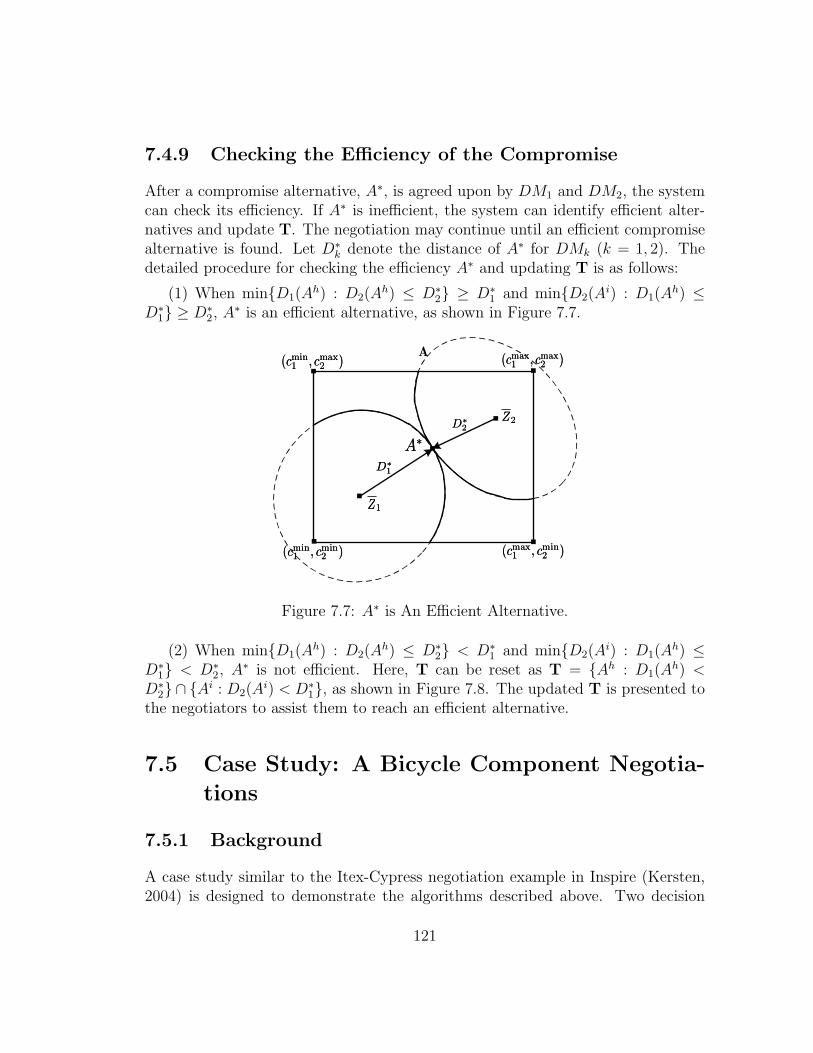
7.4.9 Checking the Efficiency of the Compromise
After a compromise alternative, A∗, is agreed upon by DM1 and DM2, the systemcan check its efficiency. If A∗ is inefficient, the system can identify efficient alter-natives and update T. The negotiation may continue until an efficient compromisealternative is found. Let D∗
k denote the distance of A∗ for DMk (k = 1, 2). Thedetailed procedure for checking the efficiency A∗ and updating T is as follows:
(1) When min{D1(Ah) : D2(A
h) ≤ D∗2} ≥ D∗
1 and min{D2(Ai) : D1(A
h) ≤D∗
1} ≥ D∗2, A∗ is an efficient alternative, as shown in Figure 7.7.
A
.
.
(cmin1, cmin2)(cmin
1, cmin2)
(cmin1, cmax2
)(cmin1, cmax2
).
(cmax1
, cmax2
)(cmax1
, cmax2
)
(cmax1
, cmin2)(cmax
1, cmin2)
.
.
.
Z1Z1
Z2Z2
.AA
D1
D1
D2
D2
Figure 7.7: A∗ is An Efficient Alternative.
(2) When min{D1(Ah) : D2(A
h) ≤ D∗2} < D∗
1 and min{D2(Ai) : D1(A
h) ≤D∗
1} < D∗2, A∗ is not efficient. Here, T can be reset as T = {Ah : D1(A
h) <D∗
2} ∩ {Ai : D2(Ai) < D∗
1}, as shown in Figure 7.8. The updated T is presented tothe negotiators to assist them to reach an efficient alternative.
7.5 Case Study: A Bicycle Component Negotia-
tions
7.5.1 Background
A case study similar to the Itex-Cypress negotiation example in Inspire (Kersten,2004) is designed to demonstrate the algorithms described above. Two decision
121
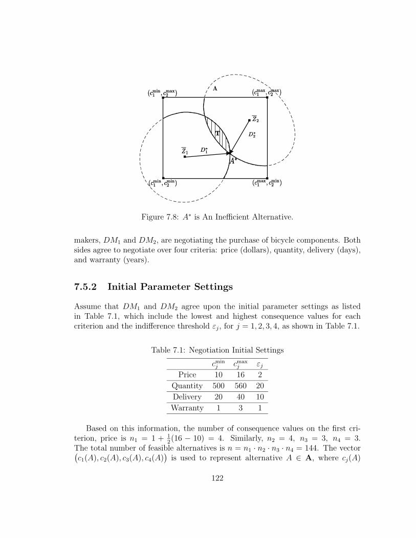
A
.
.
(cmin1, cmin2)(cmin
1, cmin2)
(cmin1, cmax2
)(cmin1, cmax2
).
(cmax1
, cmax2
)(cmax1
, cmax2
)
(cmax1
, cmin2)(cmax
1, cmin2)
.
.
.
Z1Z1
Z2Z2
TT
D1
D1
AA
D2
D2
.
Figure 7.8: A∗ is An Inefficient Alternative.
makers, DM1 and DM2, are negotiating the purchase of bicycle components. Bothsides agree to negotiate over four criteria: price (dollars), quantity, delivery (days),and warranty (years).
7.5.2 Initial Parameter Settings
Assume that DM1 and DM2 agree upon the initial parameter settings as listedin Table 7.1, which include the lowest and highest consequence values for eachcriterion and the indifference threshold εj, for j = 1, 2, 3, 4, as shown in Table 7.1.
Table 7.1: Negotiation Initial Settings
cminj cmax
j εj
Price 10 16 2
Quantity 500 560 20
Delivery 20 40 10
Warranty 1 3 1
Based on this information, the number of consequence values on the first cri-terion, price is n1 = 1 + 1
2(16 − 10) = 4. Similarly, n2 = 4, n3 = 3, n4 = 3.
The total number of feasible alternatives is n = n1 · n2 · n3 · n4 = 144. The vector(
c1(A), c2(A), c3(A), c4(A))
is used to represent alternative A ∈ A, where cj(A)
122
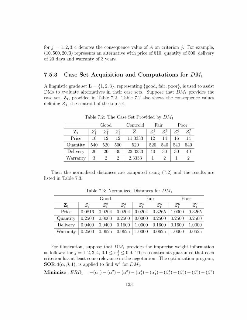
for j = 1, 2, 3, 4 denotes the consequence value of A on criterion j. For example,(10, 500, 20, 3) represents an alternative with price of $10, quantity of 500, deliveryof 20 days and warranty of 3 years.
7.5.3 Case Set Acquisition and Computations for DM1
A linguistic grade set L = {1, 2, 3}, representing {good, fair, poor}, is used to assistDMs to evaluate alternatives in their case sets. Suppose that DM1 provides thecase set, Z1, provided in Table 7.2. Table 7.2 also shows the consequence valuesdefining Z1, the centroid of the top set.
Table 7.2: The Case Set Provided by DM1
Good Centroid Fair Poor
Z1 Z11 Z2
1 Z31 Z1 Z4
1 Z51 Z6
1 Z71
Price 10 12 12 11.3333 12 14 16 14
Quantity 540 520 500 520 520 540 540 540
Delivery 20 20 30 23.3333 40 30 30 40
Warranty 3 2 2 2.3333 1 2 1 2
Then the normalized distances are computed using (7.2) and the results arelisted in Table 7.3.
Table 7.3: Normalized Distances for DM1
Good Fair Poor
Z1 Z11 Z2
1 Z31 Z4
1 Z51 Z6
1 Z71
Price 0.0816 0.0204 0.0204 0.0204 0.3265 1.0000 0.3265
Quantity 0.2500 0.0000 0.2500 0.0000 0.2500 0.2500 0.2500
Delivery 0.0400 0.0400 0.1600 1.0000 0.1600 0.1600 1.0000
Warranty 0.2500 0.0625 0.0625 1.0000 0.0625 1.0000 0.0625
For illustration, suppose that DM1 provides the imprecise weight informationas follows: for j = 1, 2, 3, 4, 0.1 ≤ w1
j ≤ 0.9. These constraints guarantee that eachcriterion has at least some relevance in the negotiation. The optimization program,SOR.4(α, β, 1), is applied to find w1 for DM1.
Minimize : ERR1 = −(α11)− (α2
1)− (α31)− (α4
1)− (α51) + (β4
1) + (β51) + (β6
1) + (β71)
123

Subject to:
{0.0816w11 + 0.2500w1
2 + 0.0400w13 + 0.2500w1
4}1/2 + α11 ≤ 1/3;
{0.0204w11 + 0.0400w1
3 + 0.0625w14}1/2 + α2
1 ≤ 1/3;
{0.0204w11 + 0.2500w1
2 + 0.1600w13 + 0.0625w1
4}1/2 + α31 ≤ 1/3;
{0.0204w11 + w1
3 + w14}1/2 + α4
1 ≤ 2/3;
{0.0204w11 + w1
3 + w14}1/2 + β4
1 ≥ 1/3;
{0.3265w11 + 0.2500w1
2 + 0.1600w13 + 0.0625w1
4}1/2 + α51 ≤ 2/3;
{0.3265w11 + 0.2500w1
2 + 0.1600w13 + 0.0625w1
4}1/2 + β51 ≥ 1/3;
{w11 + 0.2500w1
2 + 0.1600w13 + w1
4}1/2 + β61 ≥ 2/3;
{0.3265w11 + 0.2500w1
2 + w13 + 0.0625w1
4}1/2 + β71 ≥ 2/3;
−1 ≤ α11 ≤ 0; −1 ≤ α2
1 ≤ 0; −1 ≤ α31 ≤ 0; −1 ≤ α4
1 ≤ 0; −1 ≤ α51 ≤ 0;
0 ≤ β41 ≤ 1; 0 ≤ β5
1 ≤ 1; 0 ≤ β61 ≤ 1; 0 ≤ β7
1 ≤ 1;
0.1 ≤ w11 ≤ 0.9; 0.1 ≤ w1
2 ≤ 0.9; 0.1 ≤ w13 ≤ 0.9; 0.1 ≤ w1
4 ≤ 0.9;
w11 + w1
2 + w13 + w1
4 = 1;
The results of SOR.4(α, β, 1), are ERR1 = 0 and w1 = (0.5743, 0.1000, 0.2257,0.1000), which were found using Lingo (2005). Note that the error can be ignored.
7.5.4 Post-optimality Analyses for DM1
Based upon the first method described in Section 3.4, post-optimality analysis forDM1 was carried out according to the following steps:
• The post-optimality programs, SOR.4′(α, β, 1, wj) and SOR.4′′(α, β, 1, wj)were formulated for each criterion weight, w1
j . The small positive number, η,was set as 1
n= 1
144≈ 0.0069. The results are listed in Table 7.4.
• From Table 7.4, it is easy to see that the initial optimal solution (row 1)and the average values of the post-optimality analyses (last row) are close,though small variations exist. We conclude that there is no good reason todoubt the results of the program SOR.4(α, β, 1). Based upon the averagevalues of weights, the distances of all 144 alternatives in A were determined.To save space, we show in Figure 7.9 only the numbers and proportions ofalternatives in the three linguistic grades.
124
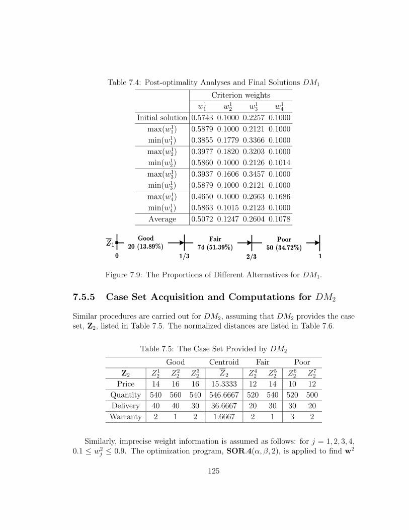
Table 7.4: Post-optimality Analyses and Final Solutions DM1
Criterion weights
w11 w1
2 w13 w1
4
Initial solution 0.5743 0.1000 0.2257 0.1000
max(w11) 0.5879 0.1000 0.2121 0.1000
min(w11) 0.3855 0.1779 0.3366 0.1000
max(w12) 0.3977 0.1820 0.3203 0.1000
min(w12) 0.5860 0.1000 0.2126 0.1014
max(w13) 0.3937 0.1606 0.3457 0.1000
min(w13) 0.5879 0.1000 0.2121 0.1000
max(w14) 0.4650 0.1000 0.2663 0.1686
min(w14) 0.5863 0.1015 0.2123 0.1000
Average 0.5072 0.1247 0.2604 0.1078
Z1Z1 .
1/30 2/3 1
Good20 (13.89%)
Fair74 (51.39%)
Poor50 (34.72%)
Figure 7.9: The Proportions of Different Alternatives for DM1.
7.5.5 Case Set Acquisition and Computations for DM2
Similar procedures are carried out for DM2, assuming that DM2 provides the caseset, Z2, listed in Table 7.5. The normalized distances are listed in Table 7.6.
Table 7.5: The Case Set Provided by DM2
Good Centroid Fair Poor
Z2 Z12 Z2
2 Z32 Z2 Z4
2 Z52 Z6
2 Z72
Price 14 16 16 15.3333 12 14 10 12
Quantity 540 560 540 546.6667 520 540 520 500
Delivery 40 40 30 36.6667 20 30 30 20
Warranty 2 1 2 1.6667 2 1 3 2
Similarly, imprecise weight information is assumed as follows: for j = 1, 2, 3, 4,0.1 ≤ w2
j ≤ 0.9. The optimization program, SOR.4(α, β, 2), is applied to find w2
125
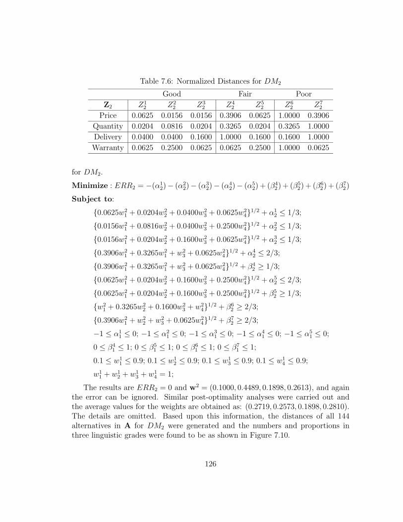
Table 7.6: Normalized Distances for DM2
Good Fair Poor
Z2 Z12 Z2
2 Z32 Z4
2 Z52 Z6
2 Z72
Price 0.0625 0.0156 0.0156 0.3906 0.0625 1.0000 0.3906
Quantity 0.0204 0.0816 0.0204 0.3265 0.0204 0.3265 1.0000
Delivery 0.0400 0.0400 0.1600 1.0000 0.1600 0.1600 1.0000
Warranty 0.0625 0.2500 0.0625 0.0625 0.2500 1.0000 0.0625
for DM2.
Minimize : ERR2 = −(α12)− (α2
2)− (α32)− (α4
2)− (α52) + (β4
2) + (β52) + (β6
2) + (β72)
Subject to:
{0.0625w21 + 0.0204w2
2 + 0.0400w23 + 0.0625w2
4}1/2 + α12 ≤ 1/3;
{0.0156w21 + 0.0816w2
2 + 0.0400w23 + 0.2500w2
4}1/2 + α22 ≤ 1/3;
{0.0156w21 + 0.0204w2
2 + 0.1600w23 + 0.0625w2
4}1/2 + α32 ≤ 1/3;
{0.3906w21 + 0.3265w2
1 + w23 + 0.0625w2
4}1/2 + α42 ≤ 2/3;
{0.3906w21 + 0.3265w2
1 + w23 + 0.0625w2
4}1/2 + β42 ≥ 1/3;
{0.0625w21 + 0.0204w2
2 + 0.1600w23 + 0.2500w2
4}1/2 + α52 ≤ 2/3;
{0.0625w21 + 0.0204w2
2 + 0.1600w23 + 0.2500w2
4}1/2 + β52 ≥ 1/3;
{w21 + 0.3265w2
2 + 0.1600w23 + w2
4}1/2 + β62 ≥ 2/3;
{0.3906w21 + w2
2 + w23 + 0.0625w2
4}1/2 + β72 ≥ 2/3;
−1 ≤ α11 ≤ 0; −1 ≤ α2
1 ≤ 0; −1 ≤ α31 ≤ 0; −1 ≤ α4
1 ≤ 0; −1 ≤ α51 ≤ 0;
0 ≤ β41 ≤ 1; 0 ≤ β5
1 ≤ 1; 0 ≤ β61 ≤ 1; 0 ≤ β7
1 ≤ 1;
0.1 ≤ w11 ≤ 0.9; 0.1 ≤ w1
2 ≤ 0.9; 0.1 ≤ w13 ≤ 0.9; 0.1 ≤ w1
4 ≤ 0.9;
w11 + w1
2 + w13 + w1
4 = 1;
The results are ERR2 = 0 and w2 = (0.1000, 0.4489, 0.1898, 0.2613), and againthe error can be ignored. Similar post-optimality analyses were carried out andthe average values for the weights are obtained as: (0.2719, 0.2573, 0.1898, 0.2810).The details are omitted. Based upon this information, the distances of all 144alternatives in A for DM2 were generated and the numbers and proportions inthree linguistic grades were found to be as shown in Figure 7.10.
126
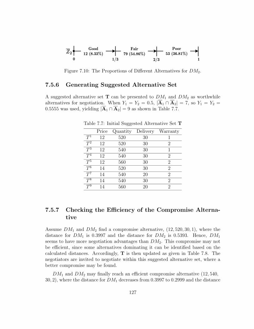
Z2Z2 .
1/30 2/3 1
Good12 (8.33%)
Fair79 (54.86%)
Poor53 (36.81%)
Figure 7.10: The Proportions of Different Alternatives for DM2.
7.5.6 Generating Suggested Alternative Set
A suggested alternative set T can be presented to DM1 and DM2 as worthwhilealternatives for negotiation. When Y1 = Y2 = 0.5, |A1 ∩ A2| = 7, so Y1 = Y2 =0.5555 was used, yielding |A1 ∩ A2| = 9 as shown in Table 7.7.
Table 7.7: Initial Suggested Alternative Set T
Price Quantity Delivery WarrantyT 1 12 520 30 1T 2 12 520 30 2T 3 12 540 30 1T 4 12 540 30 2T 5 12 560 30 2T 6 14 520 30 2T 7 14 540 20 2T 8 14 540 30 2T 9 14 560 20 2
7.5.7 Checking the Efficiency of the Compromise Alterna-tive
Assume DM1 and DM2 find a compromise alternative, (12, 520, 30, 1), where thedistance for DM1 is 0.3997 and the distance for DM2 is 0.5393. Hence, DM1
seems to have more negotiation advantages than DM2. This compromise may notbe efficient, since some alternatives dominating it can be identified based on thecalculated distances. Accordingly, T is then updated as given in Table 7.8. Thenegotiators are invited to negotiate within this suggested alternative set, where abetter compromise may be found.
DM1 and DM2 may finally reach an efficient compromise alternative (12, 540,30, 2), where the distance for DM1 decreases from 0.3997 to 0.2999 and the distance
127
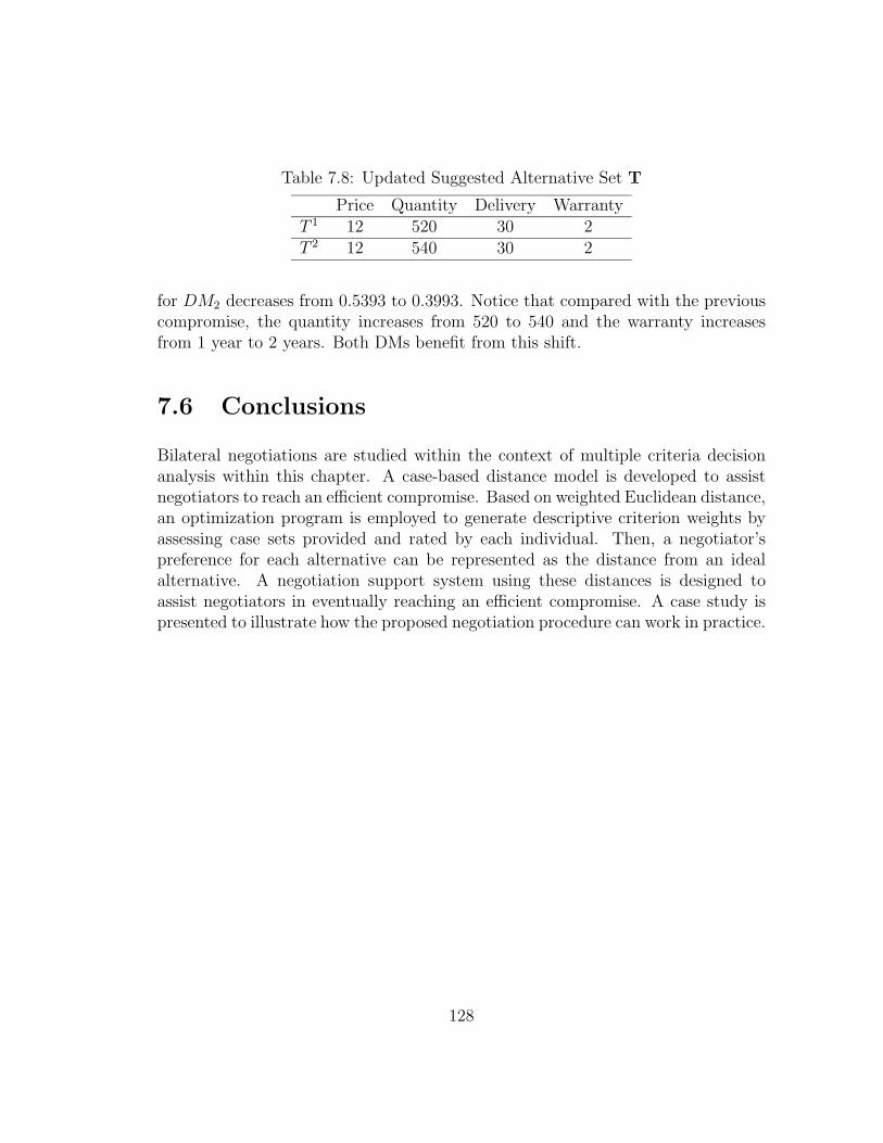
Table 7.8: Updated Suggested Alternative Set T
Price Quantity Delivery WarrantyT 1 12 520 30 2T 2 12 540 30 2
for DM2 decreases from 0.5393 to 0.3993. Notice that compared with the previouscompromise, the quantity increases from 520 to 540 and the warranty increasesfrom 1 year to 2 years. Both DMs benefit from this shift.
7.6 Conclusions
Bilateral negotiations are studied within the context of multiple criteria decisionanalysis within this chapter. A case-based distance model is developed to assistnegotiators to reach an efficient compromise. Based on weighted Euclidean distance,an optimization program is employed to generate descriptive criterion weights byassessing case sets provided and rated by each individual. Then, a negotiator’spreference for each alternative can be represented as the distance from an idealalternative. A negotiation support system using these distances is designed toassist negotiators in eventually reaching an efficient compromise. A case study ispresented to illustrate how the proposed negotiation procedure can work in practice.
128
Chapter 8
Multiple Criteria NominalClassification
8.1 Introduction
A new kind of MCDA problem, multiple criteria nominal classification (MCNC),is studied in this chapter. Traditional classification methods in MCDA focus onsorting alternatives into groups ordered by preference. MCNC is the classificationof alternatives into nominal groups, structured by the DM, who specifies multiplecharacteristics for each group. Starting with illustrative examples, the features,definition and structures of MCNC are presented, emphasizing criterion and alter-native flexibility. Then, an analysis procedure is proposed to solve MCNC prob-lems systematically. Assuming additive value functions, an optimization modelwith constraints that incorporate various classification strategies is constructed tosolve MCNC problems. An application of MCNC in water resources planning iscarried out and some future extensions are suggested. The research contained inthis chapter is founded by the work of Chen et al. (2006).
8.2 Motivation
An important variant on screening or sorting problems is the classification of al-ternatives into nominal groups, as opposed to groups ordered by preference. Suchan extension has both theoretical interest and practical applicability. For example,in human resources management, job applicants must be assigned to appropri-ate jobs, or rejected, according to their multiple qualifications (criteria). Further
129
evaluations may refine an initial assignment. We call this problem Multiple Crite-ria Nominal Classification (MCNC) to distinguish it from the standard (ordered)sorting problem, Multiple Criteria Sorting. Other applications of MCNC includebusiness management, environmental management and resource allocation.
So far as we know, traditional MCDA methods do not address MCNC problemsefficiently and would not be suitable without modifications. Only a few publishedpapers, such as those by Malakooti and Yang (2004); Perny (1998); Scarelli andNarula (2000) are relevant to MCNC. They apply outranking methods to solvespecial types of MCNC problems, but give no systematic analysis. Many issuesremain to be investigated; for example, there has been no detailed discussion of therelationship between alternatives and nominal groups. In this thesis, a systematicalanalysis procedure is proposed to help the DM to better understand and solveMCNC problems. Also, we believe our work will enrich research in the MCDA areaand inspire more research on multiple criteria nominal classification topics.
8.3 Features, Definition, Structures, and Proper-
ties of MCNC
8.3.1 Illustrative Examples of MCNC
It is easiest to explain MCNC using an example.
Example 1. An industrial company needs to recruit employees for positions in re-search and development, and technical support. The Human Resources Departmentreceived ten applications expressing interest in both positions. To improve his de-cision making, the manager decides to assign the applicants to two groups, thosesuitable for research development positions, and those suitable for technical sup-port. He uses the following criteria to evaluate applicants for each group as shownin Figure 8.1.
Based on the above criteria, the ten applicants, {A1, A2, ..., A10} are evaluatedand classified as shown in Figure 8.2, where A denotes the set of all applicants,A1 the set of applicants suitable for research and development, and A2 the set ofapplicants suitable for technical support. Note that the manager wants to screen outless qualified applicants and may (temporarily) assign highly qualified applicants toboth positions. So A4 does not appear in either group, while A6 and A10 appear inboth.
130
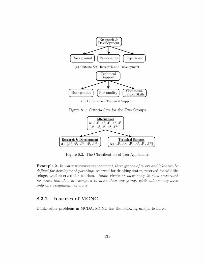
Research & Development
Background Personality Experience
(a) Criteria Set: Research and Development
Technical Support
Background Personality Communi-cation Skills
(b) Criteria Set: Technical Support
Figure 8.1: Criteria Sets for the Two Groups
AlternativesA: { A1, A2, A3, A4, A5,A6, A7, A8, A9, A10 }
Research & DevelopmentA1: {A2, A3, A6, A9, A10 }
Technical SupportA2: {A1, A5, A6, A7, A8 , A10}
Figure 8.2: The Classification of Ten Applicants
Example 2. In water resources management, three groups of rivers and lakes can bedefined for development planning: reserved for drinking water, reserved for wildliferefuge, and reserved for tourism. Some rivers or lakes may be such importantresources that they are assigned to more than one group, while others may haveonly one assignment, or none.
8.3.2 Features of MCNC
Unlike other problems in MCDA, MCNC has the following unique features:
131

Criterion Flexibility for Groups
In traditional MCDA problems, all alternatives are evaluated according to the samecriteria. This is not necessarily the case for MCNC problems, where it may notbe appropriate to apply the same criteria set to different groups. In Example 1,some criteria like Background and Personality apply to both groups, while otherslike Experience and Communication Skills are special requirements for particulargroups. Thus, MCNC can be regarded as a multiple-MCDA problem in which a setof alternatives is to be organized into groups; each group is its own MCDA problem,with its own criteria. Of course, some criteria may be common across groups, whileothers are unique to particular groups.
Alternative Flexibility for Groups
Unlike sorting problems in which each alternative belongs to only one group, inMCNC problems some alternatives may be assigned to more than one group andsome may not be assigned to any group.
8.3.3 Preliminary Definitions
Let P = (pij)n×m be an n × m matrix. Denote the transpose of P by P T . Let the
row m-vector P i denote the ith row of P . Regarding P as a column of n (row) m-vectors, we write P = (P 1, P 2, ..., P i, ..., P n)T . Let the column n-vector Pj indicatethe jth column of P. Similarly, P can be regarded as a row of m (column) n-vectors,and can be written as P = (P1, P2, ..., Pj , ..., Pm). Let Im = (1, 1, ..., 1)T be theidentity column m-vector. For a row m-vector A = (a1, a2, ..., ai, ..., am), and acolumn m-vector B = (b1, b2, ..., bi, ..., bm)T , 〈A,B〉 =
∑mi=1 ai · bi denotes the dot
product (scalar product or inner product) of A and B. Finally, define eg as the rowm-vector with 1 in the gth position and 0 elsewhere.
8.3.4 Definition and Structures of MCNC
First a formal definition of MCNC is proposed.
Multiple Criteria Classification: Definition
Definition 11. Multiple Criteria Nominal Classification (MCNC) is the assign-ment of a finite set of alternatives to nominally defined groups (subsets). Condi-
132
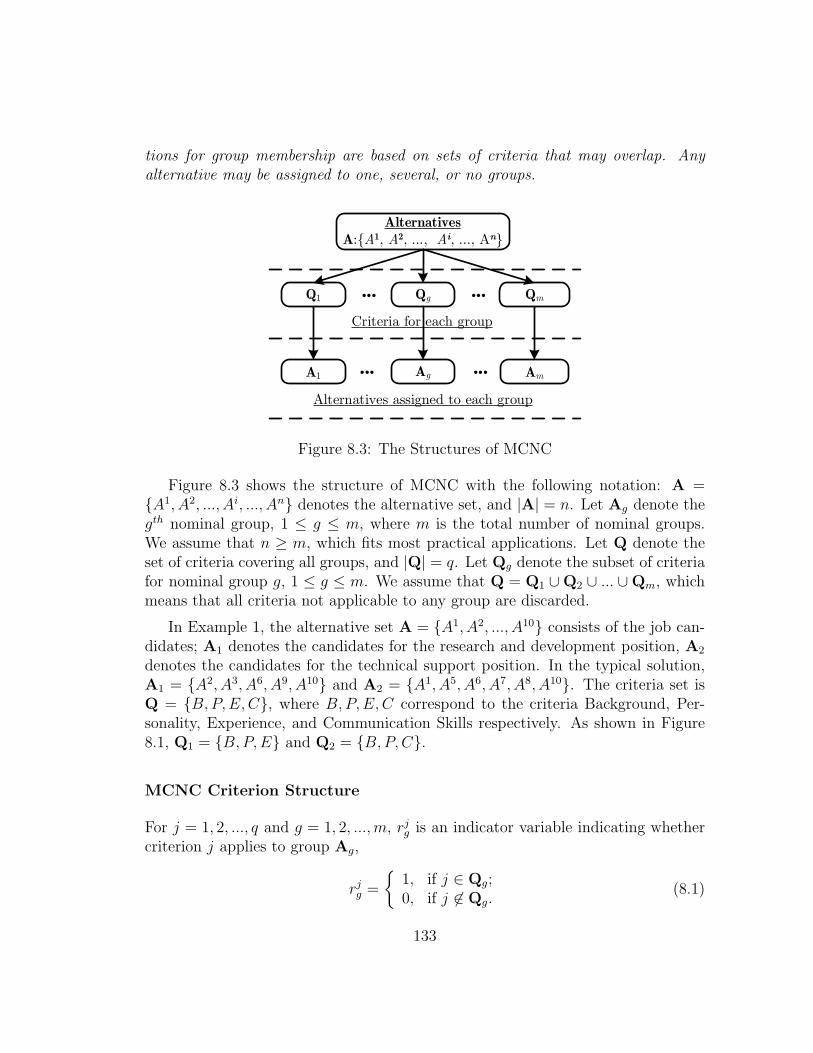
tions for group membership are based on sets of criteria that may overlap. Anyalternative may be assigned to one, several, or no groups.
Alternatives
A:{A1, A2, ..., Ai, ..., An}
Q1 QmQg... ...
... ... AmA1 Ag
Criteria for each group
Alternatives assigned to each group
Figure 8.3: The Structures of MCNC
Figure 8.3 shows the structure of MCNC with the following notation: A ={A1, A2, ..., Ai, ..., An} denotes the alternative set, and |A| = n. Let Ag denote thegth nominal group, 1 ≤ g ≤ m, where m is the total number of nominal groups.We assume that n ≥ m, which fits most practical applications. Let Q denote theset of criteria covering all groups, and |Q| = q. Let Qg denote the subset of criteriafor nominal group g, 1 ≤ g ≤ m. We assume that Q = Q1 ∪ Q2 ∪ ... ∪ Qm, whichmeans that all criteria not applicable to any group are discarded.
In Example 1, the alternative set A = {A1, A2, ..., A10} consists of the job can-didates; A1 denotes the candidates for the research and development position, A2
denotes the candidates for the technical support position. In the typical solution,A1 = {A2, A3, A6, A9, A10} and A2 = {A1, A5, A6, A7, A8, A10}. The criteria set isQ = {B,P,E,C}, where B,P,E,C correspond to the criteria Background, Per-sonality, Experience, and Communication Skills respectively. As shown in Figure8.1, Q1 = {B,P,E} and Q2 = {B,P,C}.
MCNC Criterion Structure
For j = 1, 2, ..., q and g = 1, 2, ...,m, rjg is an indicator variable indicating whether
criterion j applies to group Ag,
rjg =
{
1, if j ∈ Qg;0, if j 6∈ Qg.
(8.1)
133
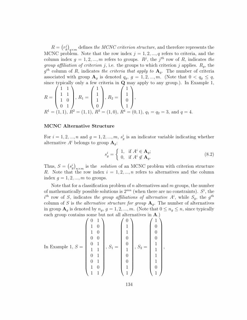
R =(
rjg
)
q×mdefines the MCNC criterion structure, and therefore represents the
MCNC problem. Note that the row index j = 1, 2, ..., q refers to criteria, and thecolumn index g = 1, 2, ...,m refers to groups. Rj, the jth row of R, indicates thegroup affiliation of criterion j, i.e. the groups to which criterion j applies. Rg, thegth column of R, indicates the criteria that apply to Ag. The number of criteriaassociated with group Ag is denoted qg, g = 1, 2, ...,m. (Note that 0 < qg ≤ q,since typically only a few criteria in Q may apply to any group.). In Example 1,
R =
1 11 11 00 1
, R1 =
1110
, R2 =
1101
,
R1 = (1, 1), R2 = (1, 1), R3 = (1, 0), R4 = (0, 1), q1 = q2 = 3, and q = 4.
MCNC Alternative Structure
For i = 1, 2, ..., n and g = 1, 2, ...,m, sig is an indicator variable indicating whether
alternative Ai belongs to group Ag:
sig =
{
1, if Ai ∈ Ag;0, if Ai 6∈ Ag.
(8.2)
Thus, S =(
sig
)
n×mis the solution of an MCNC problem with criterion structure
R. Note that the row index i = 1, 2, ..., n refers to alternatives and the columnindex g = 1, 2, ...,m to groups.
Note that for a classification problem of n alternatives and m groups, the numberof mathematically possible solutions is 2mn (when there are no constraints). Si, theith row of S, indicates the group affiliations of alternative Ai, while Sg, the gth
column of S is the alternative structure for group Ag. The number of alternativesin group Ag is denoted by ng, g = 1, 2, ...,m. (Note that 0 ≤ ng ≤ n, since typicallyeach group contains some but not all alternatives in A.)
In Example 1, S =
0 11 01 00 00 11 10 10 11 01 1
, S1 =
0110010011
, S2 =
1000111101
,
134
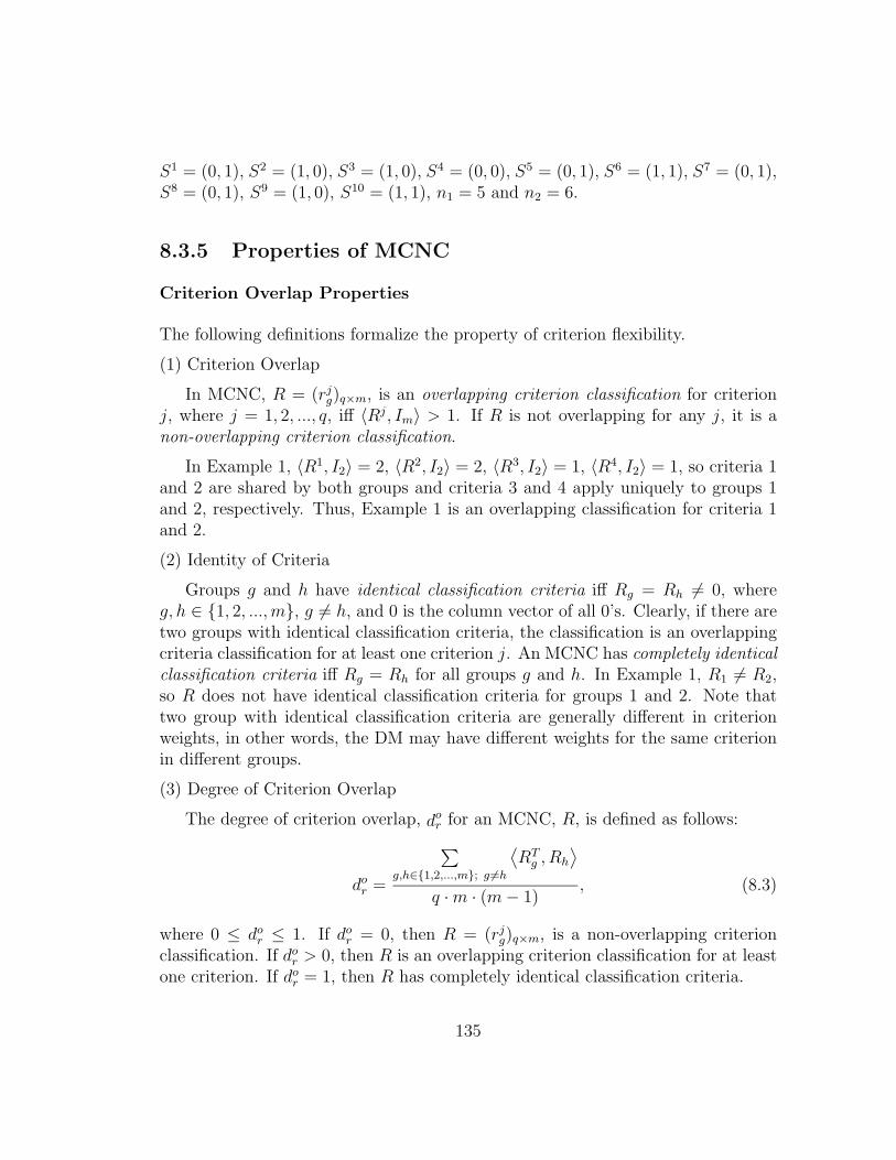
S1 = (0, 1), S2 = (1, 0), S3 = (1, 0), S4 = (0, 0), S5 = (0, 1), S6 = (1, 1), S7 = (0, 1),S8 = (0, 1), S9 = (1, 0), S10 = (1, 1), n1 = 5 and n2 = 6.
8.3.5 Properties of MCNC
Criterion Overlap Properties
The following definitions formalize the property of criterion flexibility.
(1) Criterion Overlap
In MCNC, R = (rjg)q×m, is an overlapping criterion classification for criterion
j, where j = 1, 2, ..., q, iff 〈Rj, Im〉 > 1. If R is not overlapping for any j, it is anon-overlapping criterion classification.
In Example 1, 〈R1, I2〉 = 2, 〈R2, I2〉 = 2, 〈R3, I2〉 = 1, 〈R4, I2〉 = 1, so criteria 1and 2 are shared by both groups and criteria 3 and 4 apply uniquely to groups 1and 2, respectively. Thus, Example 1 is an overlapping classification for criteria 1and 2.
(2) Identity of Criteria
Groups g and h have identical classification criteria iff Rg = Rh 6= 0, whereg, h ∈ {1, 2, ...,m}, g 6= h, and 0 is the column vector of all 0’s. Clearly, if there aretwo groups with identical classification criteria, the classification is an overlappingcriteria classification for at least one criterion j. An MCNC has completely identicalclassification criteria iff Rg = Rh for all groups g and h. In Example 1, R1 6= R2,so R does not have identical classification criteria for groups 1 and 2. Note thattwo group with identical classification criteria are generally different in criterionweights, in other words, the DM may have different weights for the same criterionin different groups.
(3) Degree of Criterion Overlap
The degree of criterion overlap, dor for an MCNC, R, is defined as follows:
dor =
∑
g,h∈{1,2,...,m}; g 6=h
⟨
RTg , Rh
⟩
q · m · (m − 1), (8.3)
where 0 ≤ dor ≤ 1. If do
r = 0, then R = (rjg)q×m, is a non-overlapping criterion
classification. If dor > 0, then R is an overlapping criterion classification for at least
one criterion. If dor = 1, then R has completely identical classification criteria.
135
In general, greater values of dor indicate higher levels of overall criteria overlap.
In Example 1, dor =
〈RT1 , R2〉+〈RT
2 , R1〉
q·m·(m−1)=
2⟨
(1,1,1,0), (1,1,0,1)T
⟩
4·2·1= 4
8= 0.5, which implies
that half of the criteria are shared.
(4) Maximum Number of Groups for a Criterion
The maximum number of groups for a criterion in an MCNC, nor is defined as
followsno
r = maxj=1,2,...,q
〈Rj, Im〉. (8.4)
In Example 1, nor = max
{
⟨
(1, 1), (1, 1)T⟩
,⟨
(1, 1), (1, 1)T⟩
,⟨
(1, 0), (1, 1)T⟩
,⟨
(1, 0),
(1, 1)T⟩
}
= max{2, 2, 1, 1} = 2, so the maximum overlap is 2, achieved by criteria
1 and 2.
(5) Criterion Correlation Between Groups
The criterion correlation of groups g and h (g, h ∈ {1, 2, ...,m}, g 6= h) for anMCNC is ρr
gh and defined as follows
ρrgh =
〈RTg , Rh〉
⟨
(Rg − Rh)T , (Rg − Rh)⟩
+ 〈RTg , Rh〉
. (8.5)
Clearly, ρrgh = ρr
hg and 0 ≤ ρrgh ≤ 1. If ρr
gh = 0, group g and h have no overlappingcriteria. If ρr
gh > 0, groups g and h have overlap on at least one criterion. If ρrgh = 1,
groups g and h have the same criteria set.
The average criterion correlation for Q is defined as
ρrQ =
∑
g,h=1,2,...,m; g 6=h
ρrgh
m · (m − 1), (8.6)
where 0 ≤ ρrQ ≤ 1. If ρr
Q = 0, then R is a non-overlapping criterion classification.If ρr
Q > 0, R is an overlapping criterion classification for at least one criterion. IfρrQ = 1, R has completely identical classification criteria.
In general, greater values of ρrQ indicate higher overall criterion overlap. In
Example 1, ρr12 = ρr
21 =
⟨
(1,1,1,0),(1,1,0,1)T
⟩
⟨(
(1,1,1,0)−(1,1,0,1))
,(
(1,1,1,0)−(1,1,0,1))T⟩
+⟨
(1,1,1,0),(1,1,0,1)T
⟩ =
24
= 0.5. Since there are only two groups, dor = ρr
gh = ρrQ = 0.5.
136
Alternative Overlap Properties
Similar definitions formalize the properties of alternative flexibility.
(1) Alternative Overlap
In MCNC, R is an overlapping alternative classification for alternative i ∈{1, 2, ..., n} iff 〈Si, Im〉 > 1, where Si is ith row of S. If R is not overlappingfor any i, it is a non-overlapping alternative classification.
In Example 1, 〈S6, Im〉 = 〈S10, Im〉 =⟨
(1, 1), (1, 1)T⟩
= 2, so alternative 6 and10 are assigned to both groups. Therefore, Example 1 is an overlapping alternativeclassification for alternatives 6 and 10.
(2) Identity of Groups
Groups g and h are identical classifications iff Sg = Sh 6= 0, where g, h ∈{1, 2, ...,m}, g 6= h and 0 is the column vector of all 0’s. Clearly, if there aretwo groups with identical classification alternatives, R is an overlapping alternativeclassification for at least one alternative. R is a completely identical classificationiff Sg = Sh for all groups g and h. In Example 1, S1 6= S2, so R does not exhibitany identical classification.
(3) Average Degree of Alternative Overlap
The average degree of alternatives overlap, dos, is defined as
dos =
∑
g,h=1,2,...,m; g 6=h
⟨
STg , Sh
⟩
n · m · (m − 1), (8.7)
where 0 ≤ dos ≤ 1. If do
s = 0, then R, is a non-overlapping alternative classification.If do
s > 0, then R is an overlapping classification for some alternatives. If dos = 1,
then R is a completely identical classification.
In general, greater values of dos indicate high levels of alternative overlap. In
Example 1,
dos =
〈ST1 ,S2〉+〈ST
2 ,S1〉
n·m·(m−1)=
2⟨
(0,1,1,0,0,1,0,0,1,1), (1,0,0,0,1,1,1,1,0,1)T
⟩
10·2·1= 0.2.
(4) Maximum Number of Groups for An Alternatives
The maximum number of groups for an alternative for an MCNC, nos, is defined
asno
s = maxi=1,2,...,n
〈Si, Im〉. (8.8)
137
In Example 1, nos = max
{
⟨
(0, 1), (1, 1)T⟩
,⟨
(1, 0), (1, 1)T⟩
,⟨
(1, 0), (1, 1)T⟩
,⟨
(0, 0),
(1, 1)T⟩
,⟨
(0, 1), (1, 1)T⟩
,⟨
(1, 1), (1, 1)T⟩
,⟨
(0, 1), (1, 1)T⟩
,⟨
(0, 1), (1, 1)T⟩
,⟨
(1, 0),
(1, 1)T⟩
,⟨
(1, 1), (1, 1)T⟩
}
= max{1, 1, 1, 0, 1, 2, 1, 1, 1, 2} = 2, so the maximum over-
lap is 2, which is achieved by alternatives 6 and 10.
(5) Complete Classification of Alternatives
In MCNC, R is a complete classification of alternatives iff 〈Si, Im〉 ≥ 1, for allalternatives i = 1, 2, ..., n. Otherwise, R is an incomplete classification of alterna-tives. In Example 1, 〈S4, Im〉 = 0, so Example 1 is an incomplete classification ofalternatives.
(6) Alternative Deficiency Degree
First M i, i = 1, 2, ..., n, an indicator variable, is defined as
M i =
{
1, if Ai belongs to at least one group;0, if Ai does not belong to any group.
(8.9)
Thus, M i = maxmg=1 si
g.
Then the degree of alternative deficiency, dds, is defined as follows.
dds = 1 −
∑
i=1,2,...,n
M i
n, (8.10)
where n is the size of the alternative set A. Here, 0 ≤ dds ≤ 1. If dd
s = 0, thenR is a complete classification of alternatives. If dd
s > 0, then R is an incompleteclassification of alternatives.
In general, greater values of dds indicate more unassigned alternatives. In Ex-
ample 1, M1 = M2 = M3 = M5 = M6 = M7 = M8 = M9 = M10 = 1, M4 = 0,
dds = 1 −
∑10i=1 M i
10= 0.1.
(7) Correlation of Alternatives Across Groups
In an MCNC, the correlation of alternatives of groups g and h (g, h ∈ {1, 2, ...,m},g 6= h) is ρs
gh, and defined as follows
ρsgh =
〈STg , Sh〉
⟨
(Sg − Sh)T , (Sg − Sh)⟩
+ 〈STg , Sh〉
. (8.11)
Clearly, ρsgh = ρs
hg and 0 ≤ ρsgh ≤ 1. If ρs
gh = 0, groups g and h have no overlappingalternatives. If ρs
gh > 0, groups g and h have at least one overlapping alternative.If ρs
gh = 1, groups g and h are identical classifications.
138
In general, greater values indicate higher overlap between two groups. Moreover,the average alternative correlation within A is defined as
ρsA =
∑
g,h=1,2,...,m; g 6=h
ρsgh
m · (m − 1), (8.12)
where 0 ≤ ρsA ≤ 1. If ρs
A = 0, R has no overlapping alternatives. If ρsA > 0, R is an
overlapping alternatives classification for at least one alternative. If ρsA = 1, then
R is a completely identical classification.
In general, greater values of ρsA indicate higher overall alternative overlap. In
Example 1, ρs12 = ρs
21 =〈ST
1 ,S2〉⟨
(S1−S2)T , (S1−S2)⟩
+〈ST1 ,S2〉
= 28+2
= 0.2. Since there are only
two groups, dos = ρs
gh = ρsA = 0.2.
8.3.6 Types of Classification
Based on alternative flexibility features, four types of multiple criteria classificationcan be distinguished, as shown in Table 8.1.
Table 8.1: MCNC Problems Classification
NOVLP OVLPCMPL MCNC1 MCNC2
INCMPL MCNC3 MCNC4
MCNC1 is an MCNC situation with non-overlapping alternatives classification(NOVLP) and complete classification of alternatives (CMPL). In this type of clas-sification, each alternative is assigned to one group only. For example, in a sportcompetition each athlete may be constrained to participate in exactly one sport.
MCNC2 is an MCNC problem with overlapping alternatives classification (OVLP)and CMPL. This type of classification requires each alternative to be assigned toat least one group. For instance, each athlete on the team can take part in one ormore sports (so that excellent athletes may compete in more than one sport).
MCNC3 is an MCNC situation with NOVLP and incomplete classification ofalternatives (INCMPL). This type of classification refers to the assignment of eachalternative to at most one group. For example, there may be a regulation that an
139
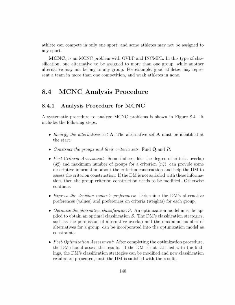
athlete can compete in only one sport, and some athletes may not be assigned toany sport.
MCNC4 is an MCNC problem with OVLP and INCMPL. In this type of clas-sification, one alternative to be assigned to more than one group, while anotheralternative may not belong to any group. For example, good athletes may repre-sent a team in more than one competition, and weak athletes in none.
8.4 MCNC Analysis Procedure
8.4.1 Analysis Procedure for MCNC
A systematic procedure to analyze MCNC problems is shown in Figure 8.4. Itincludes the following steps.
• Identify the alternatives set A: The alternative set A must be identified atthe start.
• Construct the groups and their criteria sets: Find Q and R.
• Post-Criteria Assessment: Some indices, like the degree of criteria overlap(do
r) and maximum number of groups for a criterion (nor), can provide some
descriptive information about the criterion construction and help the DM toassess the criterion construction. If the DM is not satisfied with these informa-tion, then the group criterion construction needs to be modified. Otherwisecontinue.
• Express the decision maker’s preferences: Determine the DM’s alternativepreferences (values) and preferences on criteria (weights) for each group.
• Optimize the alternative classification S: An optimization model must be ap-plied to obtain an optimal classification S. The DM’s classification strategies,such as the permission of alternative overlap and the maximum number ofalternatives for a group, can be incorporated into the optimization model asconstraints.
• Post-Optimization Assessment: After completing the optimization procedure,the DM should assess the results. If the DM is not satisfied with the find-ings, the DM’s classification strategies can be modified and new classificationresults are presented, until the DM is satisfied with the results.
140
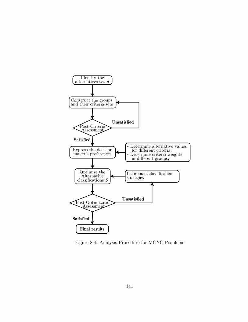
Identify the alternatives set A
Express the decision maker’s preferences
Optimize the Alternative
classifications S
Incorporate classification strategies
Post-CriteriaAssessment
Satisfied
Unsatisfied
Post-OptimizationAssessment
Final results
Satisfied
Unsatisfied
Construct the groups and their criteria sets
- Determine alternative values for different criteria;- Determine criteria weights in different groups;
Figure 8.4: Analysis Procedure for MCNC Problems
141
8.5 A Linear Additive Value Function Approach
to MCNC
8.5.1 Model Assumptions
The linear additive value function or SMART (Simple Multi-Attribute Rating Tech-nique) is a well-known approach in MCDA. Stewart (1996) argues that additivevalue functions can provide reasonable preference orderings. Hence, we propose aSMART-based optimization model to solve MCNC problems. First, some notationmust be introduced, as follows:
For g = 1, 2, ...,m, wg = (wg1, w
g2, ..., w
gj , ..., w
gq ) is the weight vector for group g.
Note that if rjg = 0, then wg
j = 0. The weights for the same criterion in different
groups may be the same (wgj = wh
j ) or not (wgj 6= wh
j ), depending on the DM’spreferences. In Example 1, the manager may place different relative importanceon the criterion of Personality in two groups. w = (w1,w2, ...,wg, ...,wm)T is theweight matrix covering all the groups.
For g = 1, 2, ...,m and i = 1, 2, ..., n, vig = (vi
1g, vi2g, ..., v
ijg, ..., v
iqg) is the value
vector of alternative Ai for group g. Note that if rjg = 0, then vi
jg = 0. Theextension of value transformation function (2.1) for MCNC problem can be set as:
vijg = fjg(c
ij) (8.13)
where fjg(·) is a mapping from consequences to values for criterion j in group g.Note that for an alternative, the values of the same criterion in different groups maybe the same (vi
jg = vijh) or not (vi
jg 6= vijh), depending on how the DM constructs
the value transformation function (8.13). We allow for the same alternative tohave different values on the same criterion in different groups. For instance, thecriterion “abundance of aquatic species” can be applied to rivers; a high level ofconsequence on this criterion is valuable in a recreation grouping, but a detrimentin a hydropower grouping.
For all alternatives, i = 1, 2, ..., n, all criteria j = 1, 2, ..., q, and all groupsg = 1, 2, ...,m,
∑
j∈Q
wgj = 1, wg
j ≥ 0; (8.14)
0 ≤ vijg ≤ 1. (8.15)
Many methods are available to obtain weights and values. With the Analytic Hi-erarchy Process (AHP) (Saaty, 1980), weights or values can be obtained by the cal-culation of eigenvalues. Swing weights is a method for direct estimation of weights
142
preferred by Belton and Stewart (2002); von Winterfeldt (1986). UTA (UTilitesAdditives) is a regression method using case studies to estimate values (Jacquet-Lagreze and Siskos, 1982). In this thesis, we assume that weights and values canbe obtained for each group without uncertainty.
8.5.2 Objective Function
Based on the SMART model assumption, the following definitions are given.
The aggregation value of alternative Ai for group g can be expressed as
V ig = 〈wg,vi
g
T 〉 =∑
j∈Q
wgj · vi
jg. (8.16)
The aggregation value vector for group g is denoted Vg = (V 1g , V 2
g , ..., V ig , ..., V n
g ).The aggregation value matrix for all groups is denoted V = (V1,V2, ...,Vg, ...,Vm)T .
The DM’s whole value for the classification solution S is denoted VS. Sincegroups are nominally defined, we assume that each group has equal importance forthe DM. Adding the aggregation values of all alternatives in all groups produces theDM’s whole value VS. The computation is implemented by the following function
VS =∑
g=1,2,...,m
eg · (V · S) · (eg)T . (8.17)
We take VS to be the objective function, so we find the best classification resultusing
maxS∈S
{VS}, (8.18)
where S denotes the set of all possible solutions of an MCNC problem.
8.5.3 Constraints
Based on the type classification chosen and some more elaborate strategies madeby the DM, some constraints need to be set for the above objective function. Thedetailed explanations are as follows.
143
Constraints for Different MCNC Types
First recall that the meanings of the following formula: (1) 〈Si, Im〉 equals the
number of groups Ai belongs to; (2)n∑
i=1
M i equals the number of all alternatives have
been assigned to at least one group; (3)
∑
{g,h=1,2,...,n; g 6=h}
⟨
STg ,Sh
⟩
n·m·(m−1)equals the average
degree of alternative overlap; and (4) 〈STg , Im〉 equals the number of alternatives
assigned to group g.
(1) MCNC1, the combination of NOVLP and CMPL, implies each alternative needto be assigned to one group only and the following constraints are set:
for all i = 1, 2, ..., n, 〈Si, Im〉 = 1 (8.19)
(2) MCNC2, the combination of OVLP and CMPL, implies each alternative to beassigned to at least one group and the following constraints are set:
for all i = 1, 2, ..., n, 〈Si, Im〉 ≥ 1, (8.20)
n∑
i=1
M i = n. (8.21)
(3) MCNC3, the combination of NOVLP and INCMPL, implies each alternativeto be assigned to at most one group and some alternatives are not assigned to anygroup. The following constraints are set:
for all i = 1, 2, ..., n, 0 ≤ 〈Si, Im〉 ≤ 1, (8.22)
0 <n
∑
i=1
M i < n. (8.23)
(4) MCNC4, the combination of OVLP and INCMPL implies some alternativesto be assigned to more than one group, while other alternatives may not belong toany group. The following constraints are set:
0 <
n∑
i=1
M i < n, (8.24)
∑
{g,h=1,2,...,n; g 6=h}
⟨
STg , Sh
⟩
n · m · (m − 1)> 0. (8.25)
144
Classification Strategies
Moreover, the DM can implement some classification strategies as constraints toelaborate upon the classification.
(1) The maximum number of groups for an alternative, 1 ≤ nos ≤ m, can be set
with the following constraints:
for all i = 1, 2, ..., n, 〈Si, Im〉 ≤ nos. (8.26)
(2) The average degree of alternative overlap, 0 ≤ dos ≤ 1, can be specified using
the following constraint:∑
{g,h=1,2,...,m; g 6=h}
⟨
STg , Sh
⟩
n · m · (m − 1)≤ do
s. (8.27)
(3) The minimum deficiency degree of alternatives, 0 ≤ dds ≤ 1, can be specified
using the following constraint:
n∑
i=1
M i ≥ n(1 − dds). (8.28)
(4) The maximum number of alternatives for group g, ng can be specified as follows:
〈STg , Im〉 ≤ ng. (8.29)
8.6 Numerical Example: Water Supply Planning
8.6.1 Problem Descriptions
Due to increases in residential, industrial, and commercial demand for water anddecreases in the reliability of groundwater resources, a city needs to develop a longterm water supply planning. The following decision process was stipulated by theRegion Council to design and implement the best resources plan:
1. Near-future Project: an immediate construction project to be completed tomeet water demands in the near future.
2. Mid-term Project: another construction project to be built between the years2018 and 2020 to meet water demands over the middle term.
145
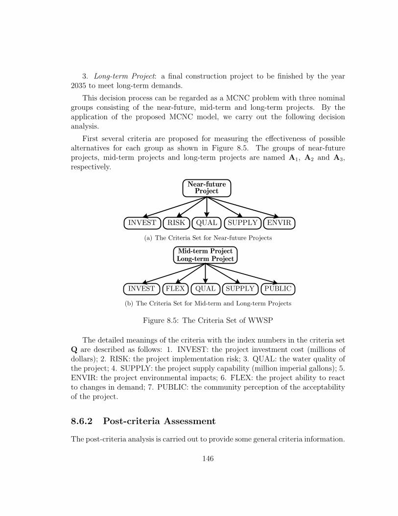
3. Long-term Project: a final construction project to be finished by the year2035 to meet long-term demands.
This decision process can be regarded as a MCNC problem with three nominalgroups consisting of the near-future, mid-term and long-term projects. By theapplication of the proposed MCNC model, we carry out the following decisionanalysis.
First several criteria are proposed for measuring the effectiveness of possiblealternatives for each group as shown in Figure 8.5. The groups of near-futureprojects, mid-term projects and long-term projects are named A1, A2 and A3,respectively.
Near-future Project
INVEST RISK QUAL ENVIRSUPPLY
(a) The Criteria Set for Near-future Projects
Mid-term ProjectLong-term Project
INVEST FLEX QUAL PUBLICSUPPLY
(b) The Criteria Set for Mid-term and Long-term Projects
Figure 8.5: The Criteria Set of WWSP
The detailed meanings of the criteria with the index numbers in the criteria setQ are described as follows: 1. INVEST: the project investment cost (millions ofdollars); 2. RISK: the project implementation risk; 3. QUAL: the water quality ofthe project; 4. SUPPLY: the project supply capability (million imperial gallons); 5.ENVIR: the project environmental impacts; 6. FLEX: the project ability to reactto changes in demand; 7. PUBLIC: the community perception of the acceptabilityof the project.
8.6.2 Post-criteria Assessment
The post-criteria analysis is carried out to provide some general criteria information.
146
|A| = 10, and m = 3 for the set {A1,A2,A3}.Q = {1, 2, ..., j, ..., 7}, |Q| = 7.
R =
1 1 11 0 01 1 11 1 11 0 00 1 10 1 1
, R1 =
1111100
, R2 =
1011011
, R3 =
1011011
.
R1 = ( 1 1 1 ), R2 = ( 1 0 0 ), R3 = ( 1 1 1 ), R4 = ( 1 1 1 ),R5 = ( 1 0 0 ), R6 = ( 0 1 1 ), R7 = ( 0 1 1 ).
dor =
2(
〈RT1 ,R2〉+〈RT
1 ,R3〉+〈RT2 ,R3〉
)
7·3·2= 11
21= 52.4%.
nor = max
(
〈R1, I3〉, 〈R2, I3〉, 〈R3, I3〉, 〈R4, I3〉, 〈R5, I3〉, 〈R6, I3〉, 〈R7, I3〉)
= 3.
ρr12 =
〈RT1 ,R2〉
⟨
(R1−R2)T , (R1−R2)⟩
+〈RT1 ,R2〉
= 37
= 42.9% = ρr13, ρr
23 = 100%.
ρrQ =
∑
{g,h=1,2,...,7;g 6=h}
ρrgh
m·(m−1)=
2·[ 37·2+1]
3·2= 13
21= 61.9%.
The criteria overlapping in this MCNC is high since dor = 52.5%, ρr
Q = 61.9%,and no
r = 3. The largest contribution of overlapping comes from Groups 2 and3, since ρr
23 = 100% (they have identical classification criteria). Although there ishigh overlapping, the criterion structure is reasonable, since we believe that suchcriterion structure can represent most of the concerns of both local residents andwater resource management experts. Note that we will show later that the differencebetween a mid-term project and long-term project is caused by different criterionweights. Different weights assigned to the same criterion in these two projectsrepresents different concerns regarding the criteria.
8.6.3 Alternative Identification
Ten alternatives have been identified. Table 8.2 shows the consequences for theMCDA problem. SUPPLY, QUAL, PUBLIC, and FLEX are identified as positivepreference criteria (the greater the consequence, the better, as indicated by “+”in Table 8.2); others are negative preference criteria (the less the consequence, thebetter, as indicated by “-” in Table 8.2).
147
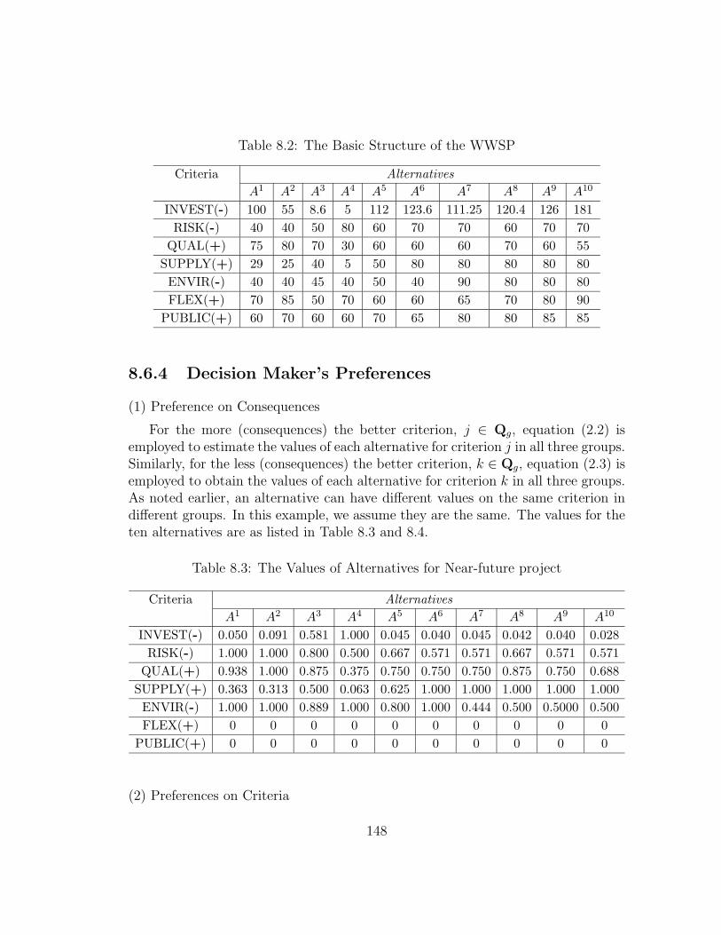
Table 8.2: The Basic Structure of the WWSP
Criteria Alternatives
A1 A2 A3 A4 A5 A6 A7 A8 A9 A10
INVEST(-) 100 55 8.6 5 112 123.6 111.25 120.4 126 181
RISK(-) 40 40 50 80 60 70 70 60 70 70
QUAL(+) 75 80 70 30 60 60 60 70 60 55
SUPPLY(+) 29 25 40 5 50 80 80 80 80 80
ENVIR(-) 40 40 45 40 50 40 90 80 80 80
FLEX(+) 70 85 50 70 60 60 65 70 80 90
PUBLIC(+) 60 70 60 60 70 65 80 80 85 85
8.6.4 Decision Maker’s Preferences
(1) Preference on Consequences
For the more (consequences) the better criterion, j ∈ Qg, equation (2.2) isemployed to estimate the values of each alternative for criterion j in all three groups.Similarly, for the less (consequences) the better criterion, k ∈ Qg, equation (2.3) isemployed to obtain the values of each alternative for criterion k in all three groups.As noted earlier, an alternative can have different values on the same criterion indifferent groups. In this example, we assume they are the same. The values for theten alternatives are as listed in Table 8.3 and 8.4.
Table 8.3: The Values of Alternatives for Near-future project
Criteria Alternatives
A1 A2 A3 A4 A5 A6 A7 A8 A9 A10
INVEST(-) 0.050 0.091 0.581 1.000 0.045 0.040 0.045 0.042 0.040 0.028
RISK(-) 1.000 1.000 0.800 0.500 0.667 0.571 0.571 0.667 0.571 0.571
QUAL(+) 0.938 1.000 0.875 0.375 0.750 0.750 0.750 0.875 0.750 0.688
SUPPLY(+) 0.363 0.313 0.500 0.063 0.625 1.000 1.000 1.000 1.000 1.000
ENVIR(-) 1.000 1.000 0.889 1.000 0.800 1.000 0.444 0.500 0.5000 0.500
FLEX(+) 0 0 0 0 0 0 0 0 0 0
PUBLIC(+) 0 0 0 0 0 0 0 0 0 0
(2) Preferences on Criteria
148
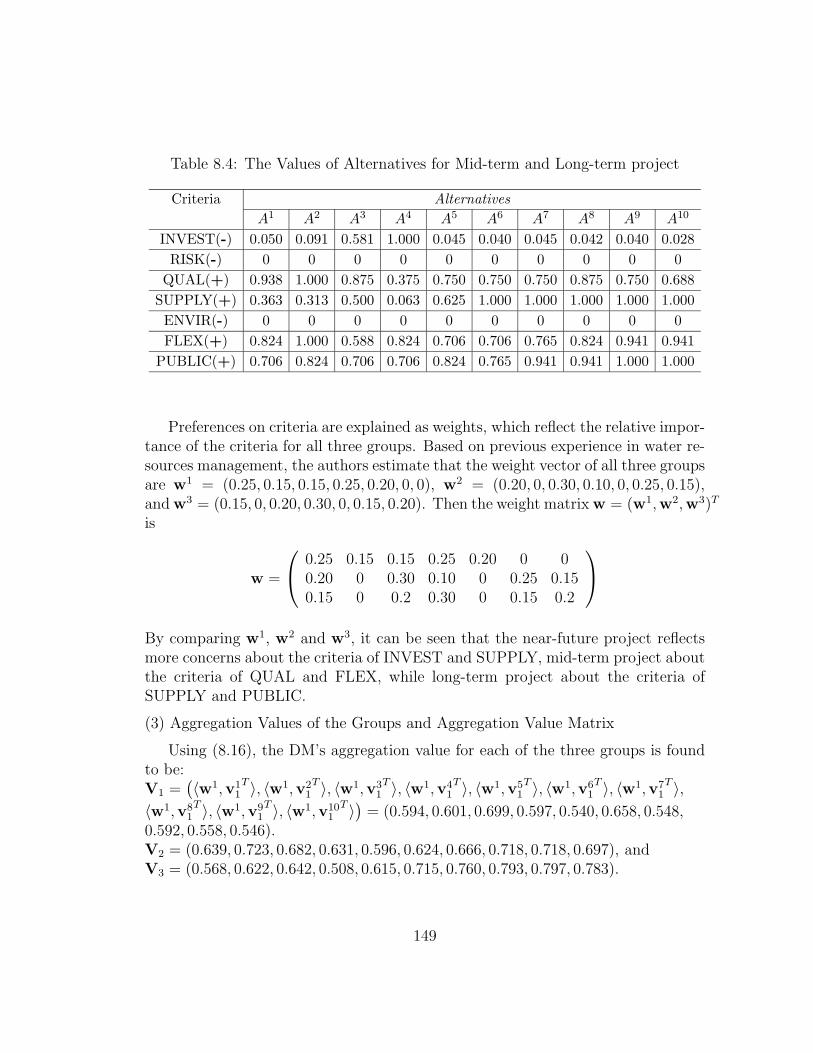
Table 8.4: The Values of Alternatives for Mid-term and Long-term project
Criteria Alternatives
A1 A2 A3 A4 A5 A6 A7 A8 A9 A10
INVEST(-) 0.050 0.091 0.581 1.000 0.045 0.040 0.045 0.042 0.040 0.028
RISK(-) 0 0 0 0 0 0 0 0 0 0
QUAL(+) 0.938 1.000 0.875 0.375 0.750 0.750 0.750 0.875 0.750 0.688
SUPPLY(+) 0.363 0.313 0.500 0.063 0.625 1.000 1.000 1.000 1.000 1.000
ENVIR(-) 0 0 0 0 0 0 0 0 0 0
FLEX(+) 0.824 1.000 0.588 0.824 0.706 0.706 0.765 0.824 0.941 0.941
PUBLIC(+) 0.706 0.824 0.706 0.706 0.824 0.765 0.941 0.941 1.000 1.000
Preferences on criteria are explained as weights, which reflect the relative impor-tance of the criteria for all three groups. Based on previous experience in water re-sources management, the authors estimate that the weight vector of all three groupsare w1 = (0.25, 0.15, 0.15, 0.25, 0.20, 0, 0), w2 = (0.20, 0, 0.30, 0.10, 0, 0.25, 0.15),and w3 = (0.15, 0, 0.20, 0.30, 0, 0.15, 0.20). Then the weight matrix w = (w1,w2,w3)T
is
w =
0.25 0.15 0.15 0.25 0.20 0 00.20 0 0.30 0.10 0 0.25 0.150.15 0 0.2 0.30 0 0.15 0.2
By comparing w1, w2 and w3, it can be seen that the near-future project reflectsmore concerns about the criteria of INVEST and SUPPLY, mid-term project aboutthe criteria of QUAL and FLEX, while long-term project about the criteria ofSUPPLY and PUBLIC.
(3) Aggregation Values of the Groups and Aggregation Value Matrix
Using (8.16), the DM’s aggregation value for each of the three groups is foundto be:V1 =
(
〈w1,v11T 〉, 〈w1,v2
1T 〉, 〈w1,v3
1T 〉, 〈w1,v4
1T 〉, 〈w1,v5
1T 〉, 〈w1,v6
1T 〉, 〈w1,v7
1T 〉,
〈w1,v81T 〉, 〈w1,v9
1T 〉, 〈w1,v10
1T 〉
)
= (0.594, 0.601, 0.699, 0.597, 0.540, 0.658, 0.548,0.592, 0.558, 0.546).V2 = (0.639, 0.723, 0.682, 0.631, 0.596, 0.624, 0.666, 0.718, 0.718, 0.697), andV3 = (0.568, 0.622, 0.642, 0.508, 0.615, 0.715, 0.760, 0.793, 0.797, 0.783).
149
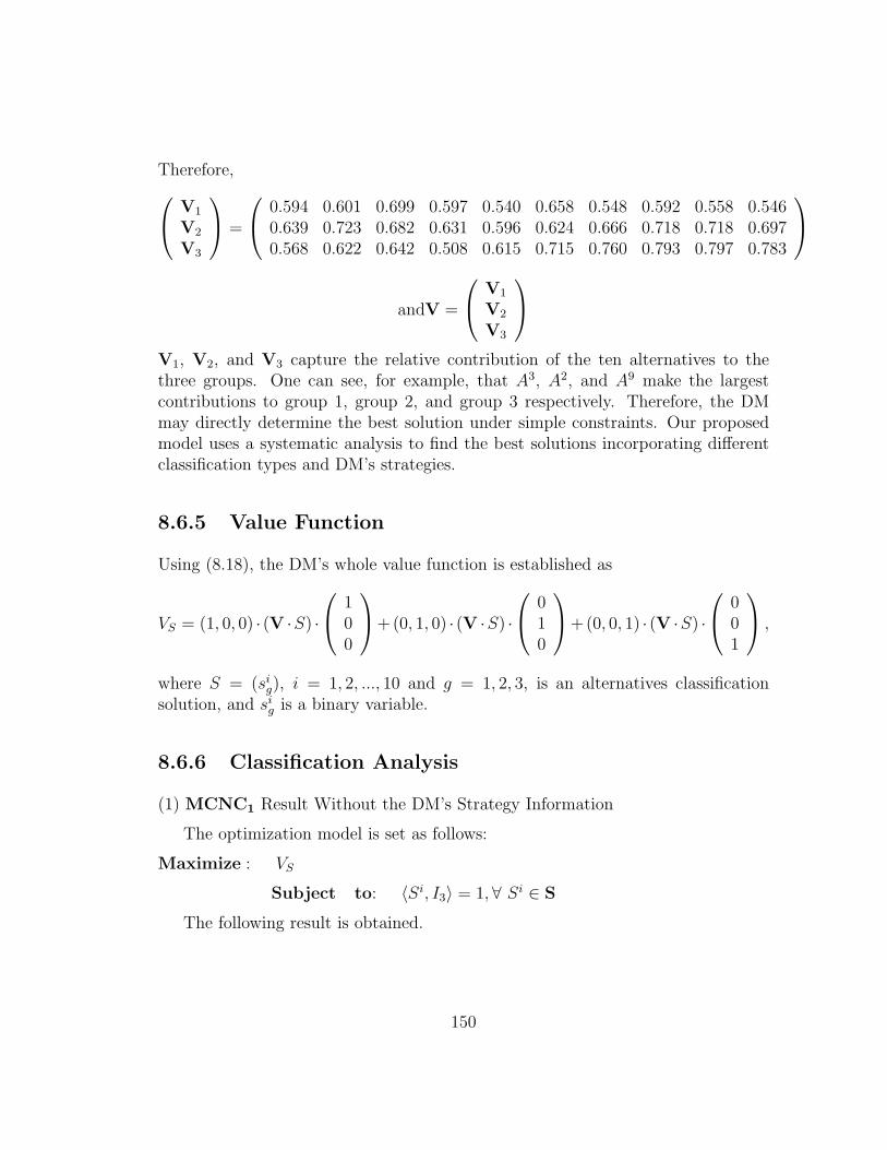
Therefore,
V1
V2
V3
=
0.594 0.601 0.699 0.597 0.540 0.658 0.548 0.592 0.558 0.5460.639 0.723 0.682 0.631 0.596 0.624 0.666 0.718 0.718 0.6970.568 0.622 0.642 0.508 0.615 0.715 0.760 0.793 0.797 0.783
andV =
V1
V2
V3
V1, V2, and V3 capture the relative contribution of the ten alternatives to thethree groups. One can see, for example, that A3, A2, and A9 make the largestcontributions to group 1, group 2, and group 3 respectively. Therefore, the DMmay directly determine the best solution under simple constraints. Our proposedmodel uses a systematic analysis to find the best solutions incorporating differentclassification types and DM’s strategies.
8.6.5 Value Function
Using (8.18), the DM’s whole value function is established as
VS = (1, 0, 0) · (V ·S) ·
100
+(0, 1, 0) · (V ·S) ·
010
+(0, 0, 1) · (V ·S) ·
001
,
where S = (sig), i = 1, 2, ..., 10 and g = 1, 2, 3, is an alternatives classification
solution, and sig is a binary variable.
8.6.6 Classification Analysis
(1) MCNC1 Result Without the DM’s Strategy Information
The optimization model is set as follows:
Maximize : VS
Subject to: 〈Si, I3〉 = 1,∀ Si ∈ S
The following result is obtained.
150
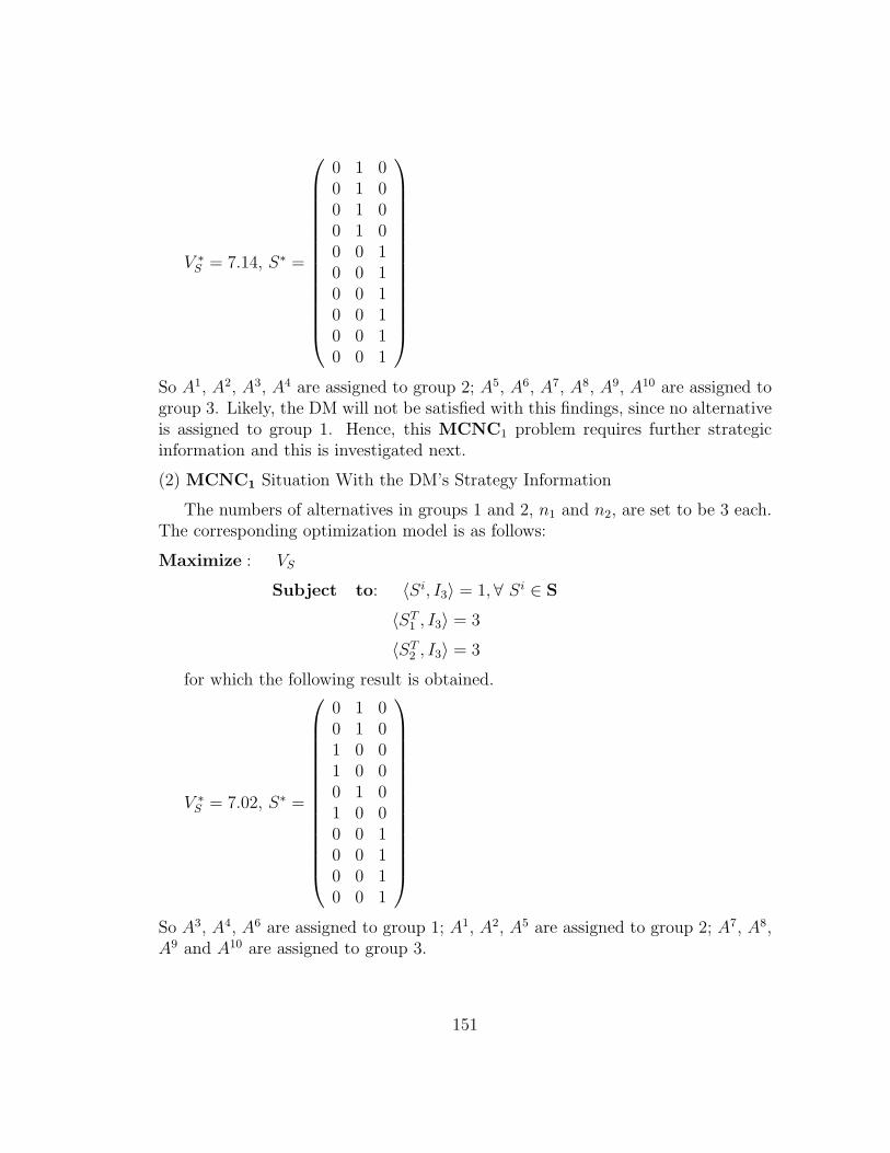
V ∗S = 7.14, S∗ =
0 1 00 1 00 1 00 1 00 0 10 0 10 0 10 0 10 0 10 0 1
So A1, A2, A3, A4 are assigned to group 2; A5, A6, A7, A8, A9, A10 are assigned togroup 3. Likely, the DM will not be satisfied with this findings, since no alternativeis assigned to group 1. Hence, this MCNC1 problem requires further strategicinformation and this is investigated next.
(2) MCNC1 Situation With the DM’s Strategy Information
The numbers of alternatives in groups 1 and 2, n1 and n2, are set to be 3 each.The corresponding optimization model is as follows:
Maximize : VS
Subject to: 〈Si, I3〉 = 1,∀ Si ∈ S
〈ST1 , I3〉 = 3
〈ST2 , I3〉 = 3
for which the following result is obtained.
V ∗S = 7.02, S∗ =
0 1 00 1 01 0 01 0 00 1 01 0 00 0 10 0 10 0 10 0 1
So A3, A4, A6 are assigned to group 1; A1, A2, A5 are assigned to group 2; A7, A8,A9 and A10 are assigned to group 3.
151
8.7 Conclusions
This research is concerned with investigating a new kind of MCDA problem, calledMultiple Criteria Nominal Classification. MCNC aims to assign alternatives tonominal groups without preferences, based on sets of criteria that may be the sameor different. The definitions, features, and properties of MCNC are stated andexplained in detail. A systematic procedure is proposed to solve MCNC problemsand an optimization model is designed that takes into account the DM’s strategiesfor the solution of MCNC problems. An application of MCNC in water supplyplanning is presented.
152
Chapter 9
Contributions and FutureResearch
Several comprehensive and flexible procedures for classification problems in MCDAhave been defined and analyzed in this thesis and many practical applications havebeen described. The main contributions of the thesis and suggestions for futureresearch are summarized in the next two subsections.
9.1 Main Contributions of the Thesis
The main contributions of this thesis are the following:
1. In Chapter 2, an analysis procedure, consequence-based preference aggrega-tion, is proposed to provide a systematic framework of MCDA. Many ap-proaches to MCDA are summarized and integrated into a meaningful struc-ture.
2. In Chapter 3, screening problems are systematically addressed: a generaldescription of a screening problem is provided, and a sequential screeningprocedure is designed to integrate several popular MCDA methods and adaptthem to solve screening problems. A case study in water supply planningin the Regional Municipality of Waterloo is carried out to demonstrate theproposed method.
3. In Chapter 4, a case-based distance method is proposed to solve screeningproblems. Research on case-based reasoning in MCDA is summarized. Then,
153
the assumptions of the proposed case-based distance method are explained indetail. Next, a quadratic program is constructed to find the best descriptivecriterion weights and the screening thresholds. Based on this information, adistance-based method is proposed for screening and a numerical example isused to demonstrate how the proposed method works.
4. In Chapter 5, the case-based distance method is extended to solve sortingproblems in MCDA. A general description of sorting problems is given indetail including a formal definition of sorting procedure and a relationshipdiscussion between the alternative set and the sorting group set. Based onweighted Euclidean distance, two case-based distance methods are developedfor sorting using weights and group thresholds obtained by assessment of acase set provided by a DM. Case-based sorting method I is designed for usewith cardinal criteria; its extension, case-based sorting method II, can handleboth cardinal and ordinal criteria. Optimization programs are employed tofind the most descriptive weights and group thresholds. Finally, a case studyon Canadian municipal water usage analysis is presented.
5. In Chapter 6, a case-based multiple criteria ABC analysis is proposed toimprove the traditional ABC analysis in inventory management and providemore managerial flexibility by accounting for additional criteria, such as leadtime and criticality. A case study is developed to illustrate how the procedurecan be applied; the results demonstrate that this approach is robust and canproduce sound classifications when multiple criteria are considered.
6. In Chapter 7, a case-based distance model founded on multiple criteria de-cision analysis theory is proposed for bilateral negotiations (BN) involvingmultiple issues. The unique feature of this negotiation model is that weightedEuclidean distance is employed to represent the negotiators’ preferences; acase-based distance algorithm then helps negotiators express their preferencesover different offers (alternatives) and suggests how to find better outcomes.The procedure takes advantage of the easily understood geometric meaningof Euclidean distance.
7. In Chapter 8, a new kind of MCDA problem, multiple criteria nominal clas-sification (MCNC), is studied. Traditional classification methods in MCDAfocus on sorting alternatives into groups ordered by preference. MCNC isthe classification of alternatives into nominal groups, structured by the DM,who specifies multiple characteristics for each group. Starting with illustrativeexamples, the features, definition and structures of MCNC are presented, em-phasizing criterion and alternative flexibility. Then an analysis procedure is
154
proposed to solve MCNC problems systematically. Assuming additive valuefunctions, an optimization model with constraints that incorporate variousclassification strategies is constructed to solve MCNC problems. An appli-cation of MCNC in water resources planning is carried out and some futureextensions are suggested.
As a result of both the theoretical developments and the real world applications,it is believed that this thesis has laid down the foundation of a new methodologyfor MCDA, namely, multiple criteria classification (MCC).
9.2 Suggestions for Future Research
The development of this thesis not only provides several approaches to modellingand analyzing classification problems in MCDA, but it also opens up new avenues tofurther research in MCDA. Below are some possible directions for future research.
1. Further research is required to refine the case-based distance approach toMCDA. Following are some important topics:
(a) The problem of handling or avoiding inconsistencies in the case set, whichis of crucial importance to the final result;
(b) The classification abilities of the case-based distance method with othertechniques, such as proposals of Doumpos and Zopouidis (2002).
(c) The comparison of the significance of various distance definitions, suchas city block distance (L1) versus Euclidean distance (L2), particularlyin an experimental setting such as multiple-issue negotiations.
(d) The expansion of the case-based distance approach to accommodate amultiple stakeholder scenario. For example, the case set sorting providedby different stakeholders might be aggregated so that final results reflectall stakeholders’ preferences.
2. In terms of the nominal classification problem, MCNC, procedures could bedesigned to take into account the effects of uncertainty in weights and values.Another research topic is the analysis of the DM’s strategies, since differentstrategic requirements may be incompatible. The DM may require assistanceto define the problem and construct his or her strategies. Other methods, forexample, distance-based methods, may be designed to solve MCNC problems.
155

3. A software-based decision support system (DSS) could help a DM implementthis approach easily and expeditiously. Hence, a computer-based DSS shouldbe developed to integrate the classification procedures discussed in the thesisand assist in practical applications.
156
Bibliography
Ahn, B.S. (2003), “Extending Malakooti’s Model for Ranking Multicriteria Alter-natives with Preference Strength and Partial Informaiton”, IEEE Transactionson Systems, Man and Cybernetics, Part A, vol. 33, pp. 281-287.
Associated Engineering (1994), Regional Municipality of Waterloo, Long TermWater Strategy, Phase 1 Report, Associated Engineering Group Ltd., Alberta,Canada.
Athanassopoulos, A.D. and Podinovski, V.V. (1997), “Dominance and PotentialOptimality in Multiple Criteria Decision Analysis with Imprecise Information”,Journal of the Operational research Society, vol. 48, pp. 142-150.
Barzilai, J., Cook, W.D. and Golani, B. (1987), “Consistent Weights for Judge-ments Matrices of the Relative Importance of Alternatives”, Operationa ResearchLetters, vol. 6, pp. 131-134.
Barzilai, J. and Golany, B. (1994), “AHP Rank Reversal, Normalization and Ag-gregation Rules”. INFOR, vol. 32, pp. 57-64.
Belacel, N. (2000), “Multicriteria Assigment Method PROAFTN: Methodology andMedical Application”, European Journal of Operational Research, vol. 125, pp.604-618.
Belton, V. and Stewart, T.J. (2002), Multiple Criteria Decision Analysis: An inte-grated Approch, Kluwer, Dordrecht.
Belton, V. and Vickers, S.P. (1993), “Demystifying DEA - A Visual Interactive Ap-proach Based on Multiple Criteria Analysis”, Journal of the Operational researchSociety, vol. 44, pp. 883-896.
Brams, S.J. (2003), Negotiation Games: Applying Game Theory to Bargaining andArbitration, Routledge, New York.
157
Brans, J.P., Mareschal, B. and Vincke, P. (1986), “How to Select and How toRank Projects: the PROMETHEE Method”, European Journal of OperationalResearch, vol. 24, pp. 228-238.
Brans, J.P. and Vincke, P. (1985), “A Preference Ranking Organization Method:the PROMETHEE Method for Multiple Criteria Decision-making”, ManagementScience, vol. 31, pp. 647-656.
Brandes, O.M. and Ferguson, K. (2003), “Flushing the Future? : Examining UrbanWater Use in Canada”, Research Report, POLIS Project on Ecological Gover-nance.
Chakravarty, A.K. (1981), “Multi-item Inventory Aggregation into Groups”, Jour-nal of Operational Research Society, vol. 32 (1), pp. 19-26.
Charnes, A. and Cooper, W.W. (1961), Management Models and Industrial Appli-cations of Linear Programming, Wiley, New York.
Charnes, A., Cooper, W.W. and Rhodes E.(1978), “Measuring Efficiency ofDecision-Making Units”, European Journal of Operational Research, vol. 2, pp.428-49.
Chen, S.M. (1996), “A New Method for Evaluating Weapon Systems Using FuzzySet Theory”, IEEE Transactions on Systems, Man and Cybernetics, Part A, vol.26, pp. 493-497.
Chen, Y., Hipel, K.W. and Kilgour, D.M. (2005a), “A Case-based Model for SortingProblems in Multiple Criteria Decision Analysis”, Proceedings of the 2005 IEEEInternational Conference on Systems, Man and Cybernetics, held in the HiltonWaikoloa Village, The Big Island of Hawaii, October 9-12, 2005, pp. 215-220,2005.
Chen, Y., Hipel, K.W., and Kilgour, D.M. (2005d), “Multiple Criteria Sorting UsingCase-based Distance Models with An Application in Water Resources Manage-ment”, IEEE Transactions on Systems, Man, and Cybernetics, Part A, in press.
Chen, Y., Kilgour, D.M., and Hipel, K.W. (2004), “An Integrated Approach toMultiple Criteria Decision Aid: Consequences Based Values Aggregation, the17 th International Conference on Multiple Criteria Decision Analysis, Whistler,British Columbia, Canada, August 6-11, 2004.
158
Chen, Y., Kilgour, D.M., and Hipel, K.W. (2005b), “Screening Techniques in Mul-tiple Criteria Decision Aid with An Application in Water Supply Planning”,submitted to Journal of Multi-Criteria Decision Analysis.
Chen, Y., Kilgour, D.M., and Hipel, K.W. (2005c), “A Case-based Distance Modelfor Screening in Multiple Criteria Decision Aid”, OMEGA, in press.
Chen, Y., Kilgour, D.M., and Hipel, K.W. (2005f), “A Case-based Distance Modelfor Bilateral Negotiations”, submitted to European Journal of Operational Re-search.
Chen, Y., Kilgour, D.M., and Hipel, K.W. (2006), “Multiple Criteria Classificationwith An Application in Water Resources Planning”, Computer and OperationsResearch, vol. 33(11), pp. 3301-3323, 2006.
Chen, Y., Li, K.W., Kilgour, D.M., and Hipel, K.W. (2005e),“A Case-based Dis-tance Model for Multiple Criteria ABC Analysis”, Computer and OperationsResearch, in press.
Cohen, M.A. and Ernst, R. (1988), “Multi-item Classification and Generic Inven-tory Stock Control Policies”, Production and Inventory Management Journal,vol. 29 (3), pp. 6-8.
Cook, W.D. and Kress, M.A. (1991), “Multiple Criteria Decision Model with Or-dinal Preference Data”, European Journal of Operational Research, vol. 54, pp.191-198.
Cook, W.D., Kress, M.A. and Seiford, L.M. (1996), “Data Envelopment Analysisin the Presence of Both Quantitative and Qualitative Factors”, Journal of theOperational Research Society, vol. 47, pp. 945-953.
Doumpos, M. and Zopounidis, C. (1998), “The Use of the Preference DisaggregationAnalysis in the Assessment of Financial Risks”. Fuzzy Economic Review, vol. 3(1),pp. 39-57.
Doumpos, M. and Zopounidis, C. (2002), Multicriteria Decision Aid ClassificationMethods, Kluwer, Dordrecht.
Doyle, J. and Green, R. (1993), “Data Envelopment Analysis and Multiple CriteriaDecision Making”. OMEGA, vol. 21, pp. 713-715.
Ehtamo, H., Hamalainen, R.P., Heiskanen, P., Teich, J., Verkama, M. and Zionts,S. (1999), “Generating Pareto Solutions in a Two-party Setting: Constraint Pro-posal Methods”, Management Science, vol. 45(12), pp. 1697-1709.
159
Environment Canada, Municipal Water Use Database (MUD), www.ec.gc.ca/water/en/manage/use/e data.htm (cited on January 10, 2005).
Eum, Y.S., Park, K.S. and Kim, S.H. (2001), “Establishing Dominance and Po-tential Optimality in Multi-criteria Analysis with Imprecise Weight and Value”,Computers & Operations Research, vol. 28, pp. 397-409.
Fang, L., Hipel, K.W., and Kilgour, D.M. (1993), Interactive Decision Making: TheGraph Model for Conflict Resolution, Wiley, New York.
Figueira, J., Greco, S., and Ehrgott, M. (2005), Multiple Criteria Decision Analysis:State of the Art Surveys, Springer Verlag, Boston, Dordrecht, London.
Fishburn, P.C. (1970) Utility Theory For Decision Making, Wiley, New York.
Fitzpatrick, P.M. (1995), Advanced Calculus, a Course in Mathematical Analysis,Thomson Brooks-Cole, Boston.
Flores, B.E., Olson, D.L., and Dorai,V.K. (1992), “Management of MulticriteriaInventory Classification”, Mathematical and Computer Modeling, vol. 16 (12),pp. 71-82.
Flores, B.E. and Whybark, D.C. (1986), “Multiple Criteria ABC Analysis”, In-ternational Journal of Operations and Production Management, vol. 6 (3), pp.38-46.
Flores, B.E. and Whybark, D.C. (1987), “Implementing Multiple Criteria ABCAnalysis”, Journal of Operations Management, vol. 7 (1), pp. 79-84.
Fraser, N.M. and Hipel, K.W. (1984), Conflict Analysis: Models and Resolutions,North Holland, New York.
French, S. (1986), Decision Theory: An Introduction to the Mathematics of Ratio-nality, Ellis Horwood Series in Mathematics and Its Application, Chichester.
Geoffrion, A. (1968), “Proper Efficiency and Theory of Vector Maximization”. Jour-nal of Mathematical Analysis and Applications, vol. 22, pp. 618-630.
Greco, S., Matarazzo, B. and Slowinski, R. (1996), “Rough Approximation of Pref-erence Relation by Dominance Relations”, ICS Research Report, Warsaw Uni-versity of Technology, Warsaw.
160
Greco, S., Matarazzo, B. and Slowinshi, R. (1999), “Rough Approximation of aPreference Relation by Dominance Relations”, European Journal of OperationalResearch, vol. 117(1), pp. 63-83.
Greco, S., Matarazzo, B. and Slowinski, R. (2001), “Rough Sets theory for Multi-criteria Decision Analysis”. European Journal of Operational Research, vol. 129,pp. 1-47.
Greco, S., Matarazzo, B. and Slowinski, R. (2002), “Rough Sets Methodology forSorting Problems in Presence of Multiple Attributes and Criteria”, EuropeanJournal of Operational Research, vol. 138, pp. 247-259.
Guvenir, H.A. and Erel, E. (1998), “Multicriteria Inventory Classification Using aGenetic Algorithm”, European Journal of Operational Research, vol. 105 (1), pp.29-37.
Haimes, Y.Y., Hall, W.A. and Freedman, H.T. (1975), Multiobjective Optimizationin Water Resources Systems: The Surrogate Worth Trade-off Method, ElsevierScientific Publishing Company, The Netherlands.
Hammer, P.L. (1986), “Partially Defined Boolean Functions and Cause-Effect Re-lationships”, the International Conference on Multi-Attribute Decision MakingVia OR-Based Expert Systems, University of Passau, Germany, April 1986.
Hammond, J.S., Keeney, R.L. and Raiffa, H. (1999), Smart Choices: A PracticalGuide to Making Better Decisions, Harvard Business School Publishing, Boston.
Hanne, T. (2001) Intelligent Strategies for Meta Multiple Criteria Decision Making.Kluwer, Boston.
Hazen, G.B. (1986), “Partial Information, Dominance, and Potential Optimality inMulti-Attribute Utility Theory”, Operations Research, vol. 34(2), pp. 296-310.
Herrera-Viedma, E., Herrera, F., and Chiclana, F. (2002), “A Consensus Modelfor Multiperson Decision Making with Different Reference Structures”, IEEETransactions on Systems, Man and Cybernetics, Part A, vol. 32, pp. 394 - 402.
Hipel, K.W. (Editor), “Multiple Objective Decision Making in Water Resources”,American Water Resources Association (AWRA) Monograph Series No. 18, andalso published as the February issue of Water Resources Bulletin, vol. 28, 1992.
Hipel, K.W., Radford, K.J., and Fang, L. (1993), “Multiple Participant-MultipleCriteria Decision Making”, IEEE Transactions on Systems, Man, and Cybernet-ics, Vol. 23, 4, pp. 1184-1189.
161
Hobbs, B.F. and Meierm P. (2000), Energy Decision and the Environment: A Guideto the Use of Multicriteria Methods, Kluwer, Massachusetts.
Howard, N. (1971), Paradoxes of Rationality: Theory of Metagames and PoliticalBehaviour, MIT Press, Cambridge.
Hwang, C. and Masud, A. (1979), Multiobjective Decision Making Methods andApplications, Spring-Verlag, Berlin.
Hwang, C.L. and Yoon, K. (1981), Multiple Attribute Decision Making, Spring-Verlag, Berlin.
Insua, D.R. (1990) Sensitivity Analysis in Multiple Objective Decision Making,Springer-Verlag, Berlin.”
Insua, D.R., and French, S. (1991), “A Framework for Sensitivity Analysis in Dis-crete Multi-Objective Decision Making, European Journal of Operational Re-search, vol. 54, pp. 176-190.
Jacquet-Lagreze, E. and Siskos, Y. (1982), “Assessing a Set of Additive UtilityFunctions for Multicriteria Decision-making, the UTA method”. European Jour-nal of Operational Research, vol. 10, pp. 151-164.
Jacquet-Lagreze, E. and Siskos, Y. (2001), “Preference Disaggregation: 20 yearsof MCDA Experience”, European Journal of Operational Research, vol. 130, pp.233-245.
Janssen, R. (1992), Multiobjective Decision Support for Environmental Manage-ment, Kluwer, Dordrecht.
Keeney, R.L. (1992), Value Focused Thinking: A Path to Creative Decision Making,Harvard University Press, Cambridge, Massachusetts.
Keeney, R.L. (2004), “Stimulating Creative Design Alternatives Using CustomerValues”, IEEE Transactions on Systems, Man and Cybernetics, Part C, vol. 34,pp. 450-459.
Keeney, R.L. and Raiffa, H. (1976), Decision With Multiple Objectives: Preferencesand Value Tradeoffs, Wiley, New York.
Keeney, R.L., Renn, O. and Winterfeldt, D.V. (1987), “Structuring West Germany’sEnergy Objectives”, Energy Policy, vol. 15, pp. 352-362.
162
Kersten, G.E., (1985), “NEGO-group Decision Support System”, Information andManagement, vol. 8, pp. 237-246.
Kersten, G.E. (2004), “E-negotiation Systems: Interaction of People and Technolo-gies to Resolve Conflicts”, InterNeg Working Papers, http://interneg.con-cordia.ca/interneg/research/papers/2004/08.pdf, cited on May 3, 2005.
Kersten, G.E. and Szapiro,T. (1986), “Generalized Approach to Modelling Negoti-ations”, European Journal of Operational Research, vol. 26, pp. 142-149.
Kilgour, D.M., Rajabi, S., Hipel, K.W. and Chen, Y. (2004), “Screening Alterna-tives in Multiple Criteria Subset Selection”, INFOR, vol.42(1), pp.43-60.
Koksalan, M.M., Karwan, M.H., and Zionts, S. (1984), “An Improved Methodfor Solving Multiple Criteria Problem Involving Discrete Alternatives”. IEEETransactions on Systems, Man, and Cybernetics, vol. 14, pp. 24-34.
Korhonen, P. (1988), “A Visual Reference Direction Approach to Solving DiscreteMultiple Criteria Problems”, European Journal of Operational Research, vol. 34,pp. 152-159.
Lee, K.S., Park, K.S. and Kim, S.H. (2002), “Dominance, Potential Optimality,Imprecise Information, and Hierarchical Structure in Multi-criteria Analysis”,Computers and Operations Research, vol. 29, pp. 1267-1281.
LINDO Systems, Inc., Lingo Software, http://www.lindo.com/, cited on September16, 2005.
Lootsma, F.A. (1993), “Scale Sensitivity in the Multiplicative AHP and SMART”,Journal of Multi-Criteria Decision Analysis, vol. 2, pp. 87-110.
Lootsma, F.A. (1997), Fuzzy Logic for Planning and Decision Making, Kluwer,Dordrecht.
Lootsma, F.A. (1999), Multi-critera Decision Analysis Via Ratio and DifferenceJudgement, Kluwer, Boston.
Lootsma, F.A., Mensch, T.C.A. and Vos, F.A. (1990), “Multi-criteria Analysisand Budget Reallocation in Long-term Research Planning”, European Journal ofOperational Research, vol. 47, pp. 293-305.
Lotfi, V., Stewart, T.J. and Zionts, S. (1992), “An Aspiration-level InteractiveModel for Multiple Criteria Decision Making”, Computers and Operations Re-search, vol. 19, pp. 671-681.
163
Lotov, A.V., Bushenkov, V.A. and Kamenev, G.K. (2004), Interactive DecisionMaps, Kluwer Academic Publishers, Boston, US.
MacCrimmon, K.R. (1973), “An Overview Of Multiple Objective Decision Mak-ing”, In Multiple Criteria Decision Making, J.L.Cochrance and M. Zeleny(eds.),University of South Carolina Press, Columbia, pp. 18-44.
Makowski, M. (1994), “Design and Implementation of Model-based Decision Sup-port Systems”, working Paper WP-94-86, International Institute for Applied Sys-tems Analysis, Laxenburg, Austria.
Malakooti, B. (2000), “Ranking and Screening Multiple Criteria Alternative WithPartial Informaiton and Use of Ordinal and Cardinal Strenth of Preferences”,IEEE Transactions on Systems, Man and Cybernetics, Part A, vol. 30, pp. 355-368.
Malakooti, B.and Yang, Z.Y. (2004), “Clustering and Group Selection of MultipleCriteria Alternatives With Application to Space-based Networks”, IEEE Trans-actions on Systems, Man and Cybernetics, Part B, vol. 34, pp. 40- 51.
Manski, C.F. and McFadden, D.L. (1981), Structural Analysis of Discrete Data andEconometric Applications, The MIT Press, Cambridge, US.
Massaglia, M. and Ostanello, A. (1991), “N-TOMIC: A Decision Support for Multi-criteria Segmenta-tion Problems”, International Workshop on Multicriteria De-cision Support, Lecture Notes in Economics and Mathematics Systems 356, pp.167C174. Springer-Verlag, Berlin.
Miller, G.A. (1956), “The Magical Number Seven, Plus or Minus Two: Some Limitson Our Capacity for Processing Information”, Psychological Review, vol. 63, pp.81-97.
Moshe, B. and Lerman, S.R. (1985), Discrete Choice Analysis, The MIT Press,Cambridge, US.
Mousseau, V. and Slowinski, R. (1998), “Inferring An ELECTRE TRI Model fromAssignment Examples”, Journal of Global Optimization, vol. 12, pp. 157-174.
Nijkamp, P. and Rietveld, P. (1990), Multicriteria Evaluation in Physical Planning,North-Holland, Amsterdam.
Nijkamp, P., Rietveld, P. and Voogd, H. (1983), Multicriteria Evaluation for Urbanand Regional Planning, Springer, Berlin.
164
Organisation for Economic Co-operation and Development (OECD) (1999), ThePrice of Water: Trends in OECD Countries, Paris: OECD, 1999.
Olson, D.L. (1996), Decision Aids for Selection Problems, Spring, New York.
Pareto, V. (1909), Manuel d’economie politique, Girard Briere, Paris.
Pareto, V. (1971), Mannual of Political Economy (English translation), A. M. Kel-ley Publishers, New York.
Partovi, F.Y. and Anandarajan, M. (2002), “Classifying Inventory Using An Arti-ficial Neural Network Approach”, Computer and Industrial Engineering, vol. 41,pp. 389-404.
Partovi, F.Y. and Hopton, W.E. (1994), “The Analytic Hierarchy Process as Ap-plied to Two Types of Inventory Problems”, Production and Inventory Manage-ment Journal, vol. 35 (1), pp. 13-19.
Pawlak, Z. (1982), “Rough Sets”, International Journal of Computer and Informa-tion Sciences, vol. 11, pp. 341-356.
Pawlak, Z. and Slowinski, R. (1994), “Rough Set Approach to Multi-attribute De-cision Analysis”, European Journal of Operational Research, vol. 72, pp. 443-459.
Perny, P. (1998), “Multicriteria Filtering Methods Based on Concordance / Non-discordance Principles”, Annals of Operations Research, vol. 80, pp. 137-167.
Pruitt, D. (1981), Negotiation Behavior, Academic Press, New York.
Radford, K.J. (1989), Individual and Small Group Decisions, Springer-Verlag, NewYork.
Raiffa, H., Richardson, J. and Metcalfe, D. (2002), Negotiation Analysis: The Sci-ence and Art of Collaborative Decision Making, Harvard University Press, Cam-bridge.
Rajabi, S. (1997), Multiple Criteria Subset Selection Under Interdependence of Ac-tions, Ph.D. Thesis, Department of Systems Design Engineering, University ofWaterloo, London, Ontario, Canada.
Rajabi, S., Kilgour, D.M., and Hipel, K.W. (1998), “Modelling Action-Interdependence in Multiple Criteria Decision Making”, European Journal ofOperational Research, vol. 110(3), pp. 490-508.
165
Roy, B. (1968), “Classement et choix en presence de points de vue multi-ples (la methode Eletre)”, Revue Francaise d’ Informatique et de RechercheOperationnelle, vol. 8, pp. 57-75.
Roy, B. (1985), Methodologie multicritere d’aide la decision, Economica, Paris.
Roy, B. (1996), Multicriteria Methodology for Decision Aiding, Kluwer, Dordrecht.
Ruby, D.A. (2002), Intermediate Microeconomic Theory, Digital Authoring Re-sources, Denver, US.
Saaty, T.L. (1980), Analytic Hierarchy Process, McGraw Hill, New York.
Sage, A.P. and White, C.C. (1984), “ARIADNE: A Knowledge-based InteractiveSystem for Planning and Decision Support”, IEEE Transactions on Systems,Man and Cybernetics, vol. 14, pp. 35-47.
Scarelli A, Narula S. (2000), “A Multicriteria Assignment Problem”, Journal ofMulti-criteria Decision Analysis, vol. 11, pp. 65-74.
Silver, E.A., Pyke, D.F., and Peterson, R. (1998), Inventory Management andProduction Planning and Scheduling, 3rd edition, Wiley, New York.
Siskos, Y. and Yannacopoulos, D. (1985), “UTASTAR: An Ordinal RegressionMethod for Building Additive Value Functions”, Investigacao Operacional, vol.5 (1), pp. 39-53.
Siskos, Y., Grigoroudis, E. and Matsatsinis, N.F. (2005), UTA Methods. In J.Figueira, S. Greco, and M. Ehrgott, editors, Multiple Criteria Decision Analysis:State of the Art Surveys, 297-344, Springer Verlag, Boston, Dordrecht, London.
Slowinski, R. (1992), “Intelligent Decision Support”, Handbook of Application andAdvances of the Rough Sets Theory, Kluwer, Dordrecht.
Slowinski, R. (1995), “Rough set approach to decision analysis”, AI Expert Maga-zine, vol. 10, pp. 18-25.
Slowinski, R. (2001), “Rough Set Theory for Multicriteria Decision Analysis”, Eu-ropean Journal of Operational Research, vol. 129, pp. 1-47.
Slowinski, R. and Zopounidis, C. (1995), “Application of the Rough Set Approachto Evaluation of Bankruptcy Risk”, International Journal of Intelligent Systemsin Accounting, Finance and Management, vol. 4(1), pp. 27-41.
166
Steuer, R.E. (1986), Multiple Criteria Optimization: Theory. Computation andApplication, Wiley, New York.
Stewart, T. (1992), “A Critical Survey on the Status of Multiple Criteria DecisionMaking Theory and Practice”, OMEGA, vol. 20, pp. 569-586.
Stewart, T. (1996), “Relationships Between Data Envelopment Analysis and Mul-ticriteria Decision Analysis”, Journal of the Operational Research Society, vol.47, pp. 654-665.
Train, K.E. (2003), Discrete Choice Methods with Simulation, Cambridge UniversityPress, Cambridge, UK.
Vetschera, R. (2004), “Preference Structures and Behavioral Consistency in Nego-tiations”, InterNeg Working Papers, http://interneg.concordia.ca/inter-neg/research/papers/2004/10.pdf, cited on May 3, 2005.
Vincke, Ph. (1992), Multiple Decision-Aid, Wiley, New York.
von Winterfeldt, D. (1980), “Structuring Decision Problems for Decision Analysis”.ActaPsychologica, vol. 45, pp. 71-93.
von Winterfeldt, D. and Edwards, W. (1986), Decision Analysis and BehavioralResearch, Cambridge University Press, Cambridge.
Wen, C.G. and Lee, C.S. (1998), “A Neural Network Approach to MultiobjectiveOptimization for Water Quality Management in a River Basin”, Water ResourcesReseach, vol. 34, pp. 427-436.
Waterloo Regional Council (2000), Waterloo’s Long Term Water Strategy, WaterlooRegional Council Report, E-00-027.1, Waterloo, Ontario, Canada.
White, D. (1983), “A Selection of Multiobjective Interactive Programming Meth-ods”. In multiobjective Decision Making, French, S., Hartley, G., et al. (eds),Academic Press, London, pp. 99-126.
Wierzbicki, A. (1982), “A Mathematical Bases for Satisfying Decision making”,Mathematical Programming, vol. 3, pp. 391-405.
Wierzbicki, A. (1986), “On the Completeness and Comstructiveness of ParametricCharacterizations to Vector Optimization Problems”, OR-Speaktrum, vol. 3, pp.391-405.
167
Yager, R.R. (1977), “Multiple Objective Decision-making Using Fuzzy Sets”, In-ternational Journal of Man-Machine Studies, vol. 9, pp. 375-382.
Yang, J. B. and Xu, D. L. (2002), “On the Evidential Reasoning Algorithm for Mul-tiattribute Decision Analysis With Uncertainty”, IEEE Transactions on Systems,Man and Cybernetics, Part A, vol. 32, pp. 289-304.
Yu, P.L. (1985), Multiple Criteria Decision Making, Plenum, New York.
Yu, P.L. (1995), Habitual Domains: Freeing Yourself from the Limits on Your Life,Highwater Editions, Kansas City, US.
Yu, W. (1992), Aide Multicritere la Decision Dans le Cale de la Problematiquedu Tri: Concepts, Methods et Applications, Doctoral Dissertation, Universite deParis-Dauphine, France.
Zeleny, M. (1982), Multiple Criteria Decision Making, McGraw-Hill, New York.
Zervakis, M.E., Goumas, S.K. and Rovithakis, G.A. (2004), “A Bayesian Frame-work for Multilead SMD Post-placement Quality Inspection”, IEEE Transactionson Systems, Man and Cybernetics, Part B, vol. 34, pp. 440- 453.
Zopounidis, C. and Doumpos, M. (2002), “Multicriteria Classification and SortingMethods: A Literature Review, European Journal of Operational Research, vol.138, pp. 229-246.
168