Multiple Imputation for MissingValues Through Conditional

Semiparametric Odds Ratio ModelsHui Xie

Assistant Professor

Division of Epidemiology & Biostatistics

UIC

This is a joint work with Drs. Hua Yun Chen and Yi Qian.

Multiple Imputation by OR model – p. 1/35

Outline

Review

Multiple Imputation by OR model – p. 2/35

Outline

Review

The Semiparametric OR Model (SOR)

Multiple Imputation by OR model – p. 2/35

Outline

Review

The Semiparametric OR Model (SOR)

Multiple Imputation (MI) under SOR

Multiple Imputation by OR model – p. 2/35

Outline

Review

The Semiparametric OR Model (SOR)

Multiple Imputation (MI) under SOR

A Simulation Study

Multiple Imputation by OR model – p. 2/35

Outline

Review

The Semiparametric OR Model (SOR)

Multiple Imputation (MI) under SOR

A Simulation Study

Empirical Application

Multiple Imputation by OR model – p. 2/35

Outline

Review

The Semiparametric OR Model (SOR)

Multiple Imputation (MI) under SOR

A Simulation Study

Empirical Application

Conclusion

Multiple Imputation by OR model – p. 2/35

Review: Multiple Imputation (MI)

Missing data is prevalent in practice.

Improper handling of Missing data can cause bias and loss ofefficiency.

MI (Rubin 1987) stands out as a popular method for missingdata analysis.

Softwares packages for MI

SAS Proc MI and Proc MIANALYZE, S-Plus library missing.

Stand-alone packages: MICE, IVEware.

These packages have made MI easy to apply in practicalanalysis.

Multiple Imputation by OR model – p. 3/35

Review: MI

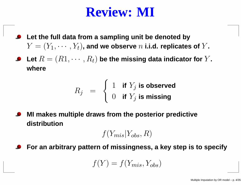
Let the full data from a sampling unit be denoted byY = (Y1, · · · , Yt), and we observe n i.i.d. replicates of Y .

Let R = (R1, · · · , Rt) be the missing data indicator for Y .where

Rj =

{

1 if Yj is observed

0 if Yj is missing

MI makes multiple draws from the posterior predictivedistribution

f(Ymis|Yobs, R)

For an arbitrary pattern of missingness, a key step is to specify

f(Y ) = f(Ymis, Yobs)

Multiple Imputation by OR model – p. 4/35

Review: MI

Common Approaches to specify f(Y )

Joint model approach. e.g. f(Y ) ∼MVN(·, ·). (e.g.impGaussian in S-Plus)

Sequential model approach (e.g. MICE in R)1: f(Y1|Y2, · · · , Yt).2: f(Y2|Y1, Y3, · · · , Yt).· · ·t: f(Yt|Y1, Y2, · · · , Yt−1).

Multiple Imputation by OR model – p. 5/35

Review: Limitations of Existing MI Software

Inflexibility in modeling mixed discrete and continuous data(Kenward and Carpenter 2007, Shafer 1997)

Joint Normal applied to discrete data.

Joint Normal have difficulties in incorporating interactionand higher order terms ( van Buuren 2007, Yu, Burton and

Rivero-Arias 2007).

Alternative Method, such as the sequential imputationapproach has limitations as follows.

Potential incompatibility in model specification ( van Buuren,

Boshuizen and Knook 1999, Raghunathan et al. 2001, Gelman an d

Raghunathan 2001).

Lack of theory to support the use of the method for MI.

Multiple Imputation by OR model – p. 6/35

A New Approach: MI under SOR

We propose a novel imputation framework for MI usingconditional Semiparametric Odds Ratio model (SOR) withthe following features.

Generalize generalized linear models (GLM).

No parametric distributional assumptions.

Flexible to model the mixture of discrete and continuousvariables.

Easily handle the bounded or semi-continuous variables, whichcan be a problem for other imputation approaches.

Simultaneously address both the issue of inflexibility of thejoint normal model and the issue of potential inconsistency ofsequential imputation models.

Multiple Imputation by OR model – p. 7/35

A New Approach: MI under SOR

We propose a novel imputation framework for MI usingconditional Semiparametric Odds Ratio model (SOR) withthe following features (cont.).

Like hot-deck approach, the proposed approach imputes amissing value by the weighted draws from the combinations ofthe observed values from different missing groups.

Unlike hot-deck approach, our imputation is model-based andis proper in Rubin’s sense.

Multiple Imputation by OR model – p. 8/35

A New Approach: MI under SOR

Outline of our work.

We study the Bayesian inference under the SOR model.

We propose using Dirichlet process prior (Ferguson 1973,1974) for nonparametric parameters in the model.

We devise an efficient posterior sampling method using Gibbssampler combined with Hybrid Monte Carlo method.

Multiple Imputation by OR model – p. 9/35

SOR model

Let the full data from a sampling unit be denoted by Y , and weobserve n i.i.d. replicates of Y . Let the density ofY = (Yt, · · · , Y1) under a product of Lebesgue measures andcount measures be decomposed into consecutive conditionaldensities as

g(yt, · · · , y1) =t∏

j=1

gj(yj |yj−1, · · · , y1).

Multiple Imputation by OR model – p. 10/35

SOR modelFor any given conditional density gj(yj |yj−1, · · · , y1), definethe odds ratio function relative to a sample point (yj0, · · · , y10)as

ηj{yj ; (yj−1, · · · , y1)|yj0, · · · , y10} =

gj(yj |yj−1, · · · , y1)/gj(yj0|yj−1, · · · , y1)

gj(yj |y(j−1)0, · · · , y10)/gj(yj0|y(j−1)0, · · · , y10).

For notational simplicity, we will use ηj{yj ; (yj−1, · · · , y1)} todenote ηj{yj ; (yj−1, · · · , y1)|yj0, · · · , y10}. Chen (2003, 2004,2007) showed that the conditional density can be rewritten as

gj(yj |yj−1, · · · , y1) =

ηj{yj ; (yj−1, · · · , y1)}gj(yj |y(j−1)0, · · · , y10)∫

ηj{yj ; (yj−1, · · · , y1)}gj(yj |y(j−1)0, · · · , y10)dyj.

Multiple Imputation by OR model – p. 11/35

SOR modelNote that

gj(yj |yj−1, · · · , y1) =

ηj{yj ; (yj−1, · · · , y1)}gj(yj |y(j−1)0, · · · , y10)∫

ηj{yj ; (yj−1, · · · , y1)}gj(yj |y(j−1)0, · · · , y10)dyj.

The SOR model decomposes gj(yj |yj−1, · · · , y1) into twoparts:

A marginal-like density function:fj(yj) = gj(yj |y(j−1)0, · · · , y10)

An odds-ratio function:ηj{yj ; (yj−1, · · · , y1)}

Multiple Imputation by OR model – p. 12/35

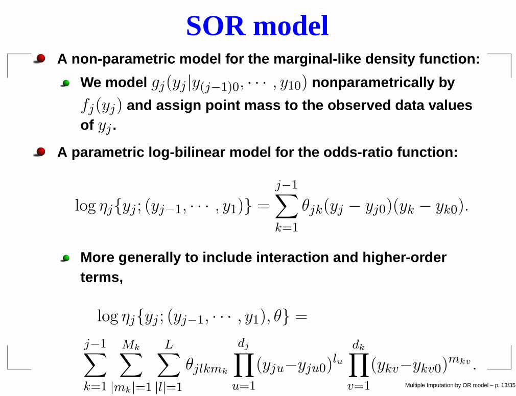
SOR modelA non-parametric model for the marginal-like density function:

We model gj(yj |y(j−1)0, · · · , y10) nonparametrically by

fj(yj) and assign point mass to the observed data valuesof yj .

A parametric log-bilinear model for the odds-ratio function:

log ηj{yj ; (yj−1, · · · , y1)} =

j−1∑

k=1

θjk(yj − yj0)(yk − yk0).

More generally to include interaction and higher-orderterms,

log ηj{yj ; (yj−1, · · · , y1), θ} =

j−1∑

k=1

Mk∑

|mk|=1

L∑

|l|=1

θjlkmk

dj∏

u=1

(yju−yju0)lu

dk∏

v=1

(ykv−ykv0)mkv .

(1)

Multiple Imputation by OR model – p. 13/35

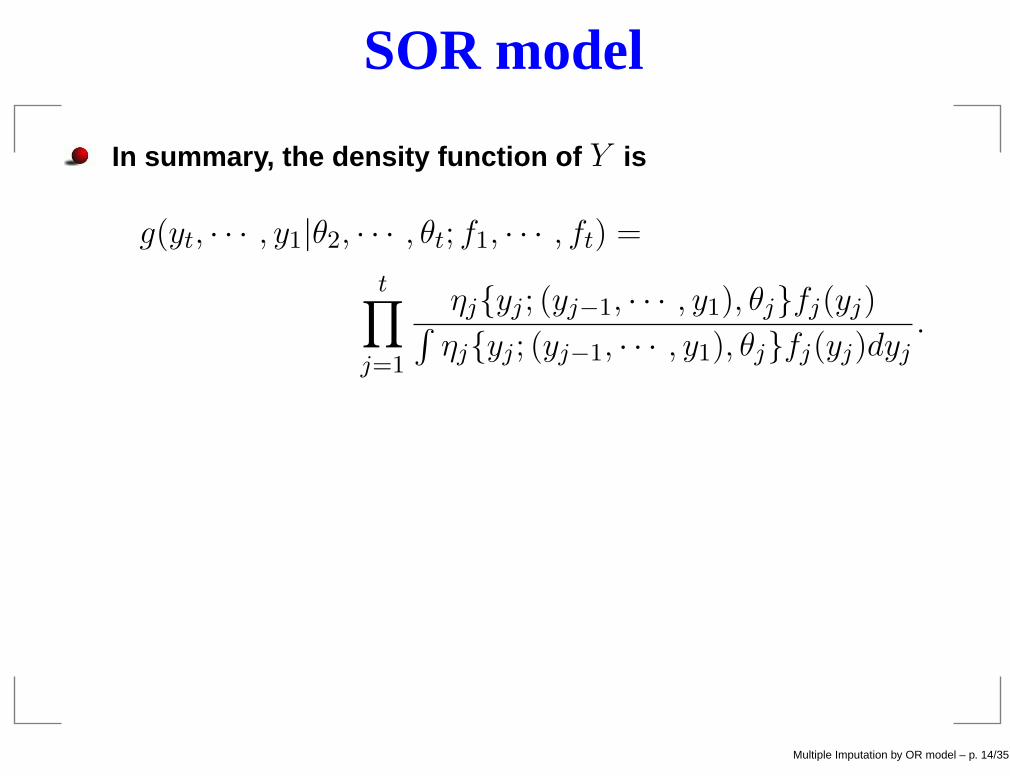
SOR model

In summary, the density function of Y is

g(yt, · · · , y1|θ2, · · · , θt; f1, · · · , ft) =

t∏

j=1

ηj{yj ; (yj−1, · · · , y1), θj}fj(yj)∫

ηj{yj ; (yj−1, · · · , y1), θj}fj(yj)dyj.

Multiple Imputation by OR model – p. 14/35

Relation to GLMSOR nests GLM.

gj(yj |yj−1, · · · , y1) = exp

[

1

φj{θjyj − b(θj)} + c(yj , φj)

]

One can show the marginal-like density is:

gj(yj |y(j−1)0, · · · , y10) = exp

[

1

φ{θj0yj − b(θj0)} + c(yj , φj)

]

.

and the odds ratio function is:

ηj{yj ; (yj−1, · · · , y1)} = exp {(yj − yj0)(θj − θj0)/φj} .

With canonical link function, θj = β0 + β1y1 + · · · + βj−1yj−1

parameters in the odds ratio function are(βk/φj , k = 1, · · · , j − 1)

Multiple Imputation by OR model – p. 15/35

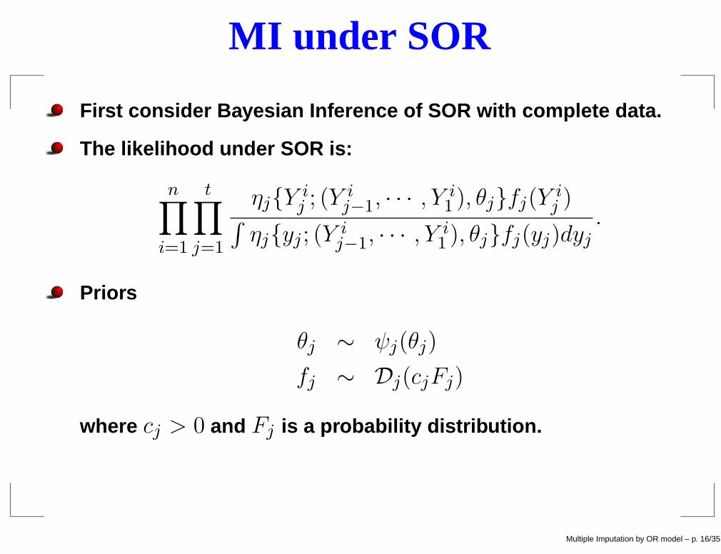
MI under SOR

First consider Bayesian Inference of SOR with complete data.

The likelihood under SOR is:

n∏

i=1

t∏

j=1

ηj{Yij ; (Y

ij−1, · · · , Y

i1 ), θj}fj(Y

ij )

∫

ηj{yj ; (Y ij−1, · · · , Yi1 ), θj}fj(yj)dyj

.

Priors

θj ∼ ψj(θj)

fj ∼ Dj(cjFj)

where cj > 0 and Fj is a probability distribution.

Multiple Imputation by OR model – p. 16/35

MI under SOR

Given the above model specification, the posterior distributionof model parameters is:

P(θj , fj |Yi, i = 1, · · · , n)

∝

{

n∏

i=1

pj(Yij |Y

ij−1, · · · , Y

i1 , θj , fj)

}

Dj(fj)ψj(θj)

∝

{

n∏

i=1

ηj{Yij ; (Y

ij−1, · · · , Y

i1 ), θj}

∫

ηj{yj ; (Y ij−1, · · · , Yi1 ), θj}fj(yj)dyj

}

ψj(θj)

· Dj

(

cjFj +n∑

i=1

δY ij

)

where δYjdenote the point measure at Yj .

Multiple Imputation by OR model – p. 17/35

MI under SOR

To simplify computation, we set the Dirichlet process prior withthe mean distribution having probability mass on the observeddata points.

This is in analogy to use the empirical distribution toapproximate the true continuous distribution when Yj iscontinuous

This is equivalent to replacing Dj(cjFj + nFnj) with

D((cj + n)Fnj), where Fnj = 1n

∑

i δY ij

. Note that

cjFj + nFnj = (cj + n)Fnj + cj(Fj − Fnj).

The second term is of lower order in n compared with the firstterm on the right-hand side of the foregoing equation. Thissuggests that the replacement is approximately right for largen.

Multiple Imputation by OR model – p. 18/35

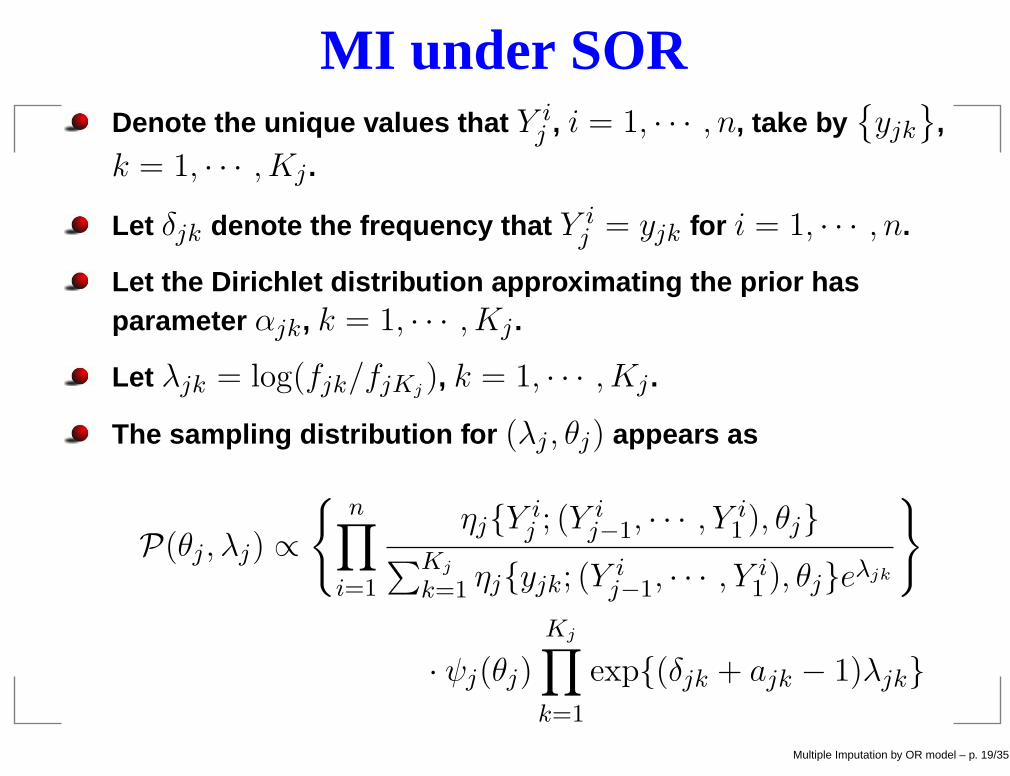
MI under SORDenote the unique values that Y ij , i = 1, · · · , n, take by

{

yjk}

,

k = 1, · · · , Kj .

Let δjk denote the frequency that Y ij = yjk for i = 1, · · · , n.

Let the Dirichlet distribution approximating the prior hasparameter αjk, k = 1, · · · , Kj .

Let λjk = log(fjk/fjKj), k = 1, · · · , Kj .

The sampling distribution for (λj , θj) appears as

P(θj , λj) ∝

{

n∏

i=1

ηj{Yij ; (Y

ij−1, · · · , Y

i1 ), θj}

∑Kj

k=1 ηj{yjk; (Yij−1, · · · , Y

i1 ), θj}eλjk

}

· ψj(θj)

Kj∏

k=1

exp{(δjk + ajk − 1)λjk}

Multiple Imputation by OR model – p. 19/35

Updating: A hybrid monte carlo (HMC) algorithm

We apply the hybrid monte carlo (Liu 2001, Chapter 9) tosample λj and θj

Let U(λj , θj) = − lnP(θj , λj) and

H{(λj , θj), (pj , qj)} = U(λj , θj)+1

2

Kj−1∑

k=1

p2jk

mjk+

Dj∑

k=1

q2jknjk

,

where (pj , qj) are auxiliary variables.

Starting from (λoldj , θoldj ), HMC uses leap-frog algorithm to

propose candidate draw (λnewj , θnewj ). The candidate sample isthen accepted with the probability

min(1,exp[−H{(λnewj ,θnew

j ),(pnewj ,qnew

j )}+H{(λoldj ,θold

j ),(poldj ,qold

j )}]).

Multiple Imputation by OR model – p. 20/35

Updating: Leap-frog Algorithm

Let (λ0j , θ

0j ) = (λoldj , θoldj ). Draw p′j from the normal

distribution with mean 0 and variance diag (mj1, ...,mj(Kj−1)),

and draw q′j from the normal distribution with mean 0 and

variance diag (nj1, ..., njDj). Then the initial momentum p0

j and

q0j have their elements given as follows:

p0jk = p′jk −

∆

2

∂U

∂λjk

{

λ0j , θ

0j

}

q0jk = q′jk −∆

2

∂U

∂θjk

{

λ0j , θ

0j

}

Multiple Imputation by OR model – p. 21/35

Updating: Leap-frog Algorithm

From the initial phase space (λ0j , θ

0j , p

0j , q

0j ) of the system, we

run the leap-frog algorithm in S steps to generate a new phase

space (λSj , θSj , p

Sj , q

Sj ) where for the s step

λsjk = λs−1jk + ∆

ps−1jk

mjk

θsjk = θs−1jk + ∆

ps−1jk

mjk

psjk = ps−1jk − ∆s

∂U

∂λjk

{

λsjk, θsjk

}

qsjk = qs−1jk − ∆s

∂U

∂θjk

{

λsjk, θsjk

}

where s = 1, ..., S, ∆s = ∆ for s < S and ∆s = ∆2 if s = S, ∆

is the user-specified stepsize, and Multiple Imputation by OR model – p. 22/35

Updating: Leap-frog Algorithm

Derivatives are:

∂U∂λjk

= −(δjk + αjk − 1) +∑n

i=1ηj{yjk;(Y i

j−1,··· ,Yi1 ),θj}e

λjkPKjk=1 ηj{yjk;(Y i

j−1,··· ,Yi1 ),θj}e

λjk

∂U∂θjk

= − ∂∂θjk

logψj(θj)−

Pn

i=1∂

∂θjklog ηj{Y

ij ;(Y i

j−1,··· ,Yi1 ),θj}

+

Pn

i=1

Kjk=1

∂∂θjk

ηj{yjk;(Y ij−1,··· ,Y i

1 ),θj}eλjk

Kjk=1

ηj{yjk;(Y ij−1

,··· ,Y i1),θj}e

λjk.

High optimal acceptance rate (65%, Beskos et al. 2010) whilebeing able to quickly explore all areas of the target distributionby exploiting the gradient information.

Multiple Imputation by OR model – p. 23/35

Updating: A hybrid monte carlo algorithm

The Gibbs sampler for sampling (λj , θj), j = 1, · · · , titeratively can be described as follows.

1. Fit an independence model to the data, which is equivalentto setting η ≡ 1 (or θ = 0) and f to the empirical marginalprobability mass function.

2. Given data, sample (θj , λj) using the hybrid monte carloapproach.

3. Do step 2 for j = 1, · · · , t.

4. Repeat steps 2 and 3 until convergence.

Multiple Imputation by OR model – p. 24/35

MI under SOR

MCMC algorithm for MI under SOR is as follows:

1. Initially, the missing values are imputed usingindependence model or from other method (e.g. MICE.).

2. Carry out one step of the hybrid monte carlo samplingalgorithm for (λj , θj), j = 1, · · · , t.

3. Draw γ from the distribution with density proportional to

P (γ|Ri,Y i,i=1,··· ,n)∝

Qn

i=1

Qr{π(r,Y i

1 ,··· ,Yi

t ,γ)}1{Ri=r}ξ(γ).

Multiple Imputation by OR model – p. 25/35

MI under SOR

MCMC algorithm for MI under SOR continued:

4. For each i = 1, · · · , n and missing group Yj , j = 1, · · · t,

if Y ij is missing, impute Y ij from the conditional distribution

of Y ij given (Y i−j , Ri, γ, θj , fj), which is the discretedistribution proportional to�

π(Ri,Yi1 ,··· ,Y

it ,γ)

Qt

l=j

ηl{Y il;(Y i

l−1,··· ,Y i1 ),θl}

ηl{yl;(Yil−1

,··· ,Y i1),θl}fl(yl)dyl

�fj(Y

ij ).

5. Repeat steps 2-4 until convergence.

Multiple Imputation by OR model – p. 26/35

A Simulation StudyWe simulated complete data from the following jointdistribution of six variables:

Y1 ∼ N(0, 1)

Given Y1, Y2 is binary with

logit {P (Y2=1|Y1)}=β20+β21Y1.

Given Y1 and Y2, Y3 is normally distributed with unitvariance and mean

µ1(Y1,Y2)=β30+β31Y1+β32Y2+β33Y1∗Y2,

Given Y1, Y2, Y3, Y4 is Poisson distributed with rateparameter

lnλ(Y1,Y2,Y3)=β40+β41Y1+β42Y2+β43Y3.

Multiple Imputation by OR model – p. 27/35

A Simulation Study

Complete data model continued:

Given Y1, · · · , Y4, Y5 is normally distributed with unitvariance and mean

µ2(Yj ,j=1,··· ,4)=β50+β51Y1+β52Y2+β53Y3+β54Y4+β55Y3∗Y4,

Given Yj , j = 1, · · · , 5, Y6 is binary with

logit {P (Y6 = 1|Yj , j = 1, · · · , 5)}

=β60+β61Y1+β62Y2+β63Y3+β64Y4+β65Y5+β66Y2∗Y4.

Two Scenarios:

No Interactions: (β33, β55, β66) = (0, 0, 0).

With Interactions: (β33, β55, β66) = (1, 1,−1).

Multiple Imputation by OR model – p. 28/35

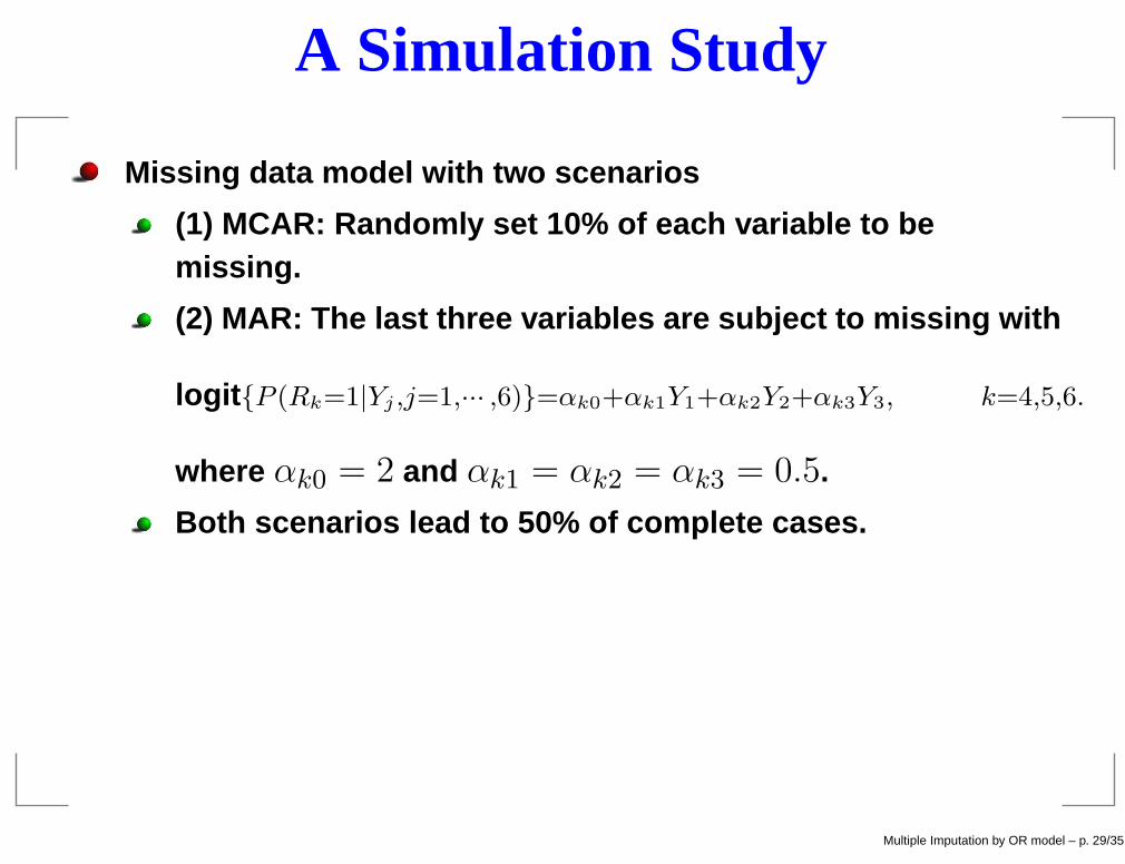
A Simulation Study

Missing data model with two scenarios

(1) MCAR: Randomly set 10% of each variable to bemissing.

(2) MAR: The last three variables are subject to missing with

logit {P (Rk=1|Yj ,j=1,··· ,6)}=αk0+αk1Y1+αk2Y2+αk3Y3, k=4,5,6.

where αk0 = 2 and αk1 = αk2 = αk3 = 0.5.

Both scenarios lead to 50% of complete cases.

Multiple Imputation by OR model – p. 29/35

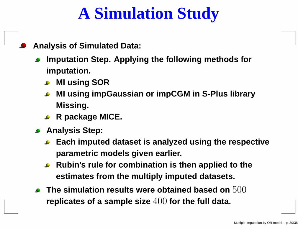
A Simulation Study

Analysis of Simulated Data:

Imputation Step. Applying the following methods forimputation.

MI using SORMI using impGaussian or impCGM in S-Plus libraryMissing.R package MICE.

Analysis Step:Each imputed dataset is analyzed using the respectiveparametric models given earlier.Rubin’s rule for combination is then applied to theestimates from the multiply imputed datasets.

The simulation results were obtained based on 500replicates of a sample size 400 for the full data.

Multiple Imputation by OR model – p. 30/35

28

Bio

metrics,

000

0000

Table 1

Simulation results for the MCAR data without interaction.

Parameter FD CC JN MICE Imp

Bias SE CR Bias SE CR Bias SE (RSE) CR Bias SE(RSE) CR Bias SE(RSE) CR

β21 = 2.0 0.01 0.20 97 0.04 0.29 96 -0.03 0.22(0.22) 96 0.01 0.22(0.22) 96 0.01 0.22 (0.22) 96

β31 = 1.0 0.00 0.06 94 0.00 0.09 94 -0.04 0.07(0.07) 94 -0.01 0.07(0.07) 95 0.00 0.07 (0.07) 95

β32 = −3.0 0.01 0.13 94 0.01 0.17 95 -0.08 0.13(0.14) 94 0.02 0.14(0.14) 94 0.02 0.14 (0.13) 94

β41 = 0.0 0.00 0.06 96 0.01 0.08 96 0.02 0.07(0.07) 94 0.01 0.07(0.07) 95 0.00 0.07 (0.07) 96

β42 = 1.0 0.00 0.15 96 -0.01 0.21 95 -0.08 0.16(0.17) 92 -0.01 0.17(0.17) 95 -0.01 0.17 (0.17) 94

β43 = 0.0 0.00 0.04 96 -0.00 0.05 96 -0.01 0.04(0.04) 94 -0.00 0.04(0.04) 94 -0.00 0.04 (0.04) 94

β51 = 0.0 0.00 0.08 95 0.00 0.12 94 -0.02 0.09(0.10) 95 0.00 0.10(0.10) 94 0.00 0.10 (0.10) 95

β52 = −1.0 -0.01 0.22 95 0.00 0.30 94 0.06 0.23(0.25) 96 -0.01 0.26(0.25) 93 -0.01 0.26 (0.25) 94

β53 = 1.0 0.00 0.05 94 0.00 0.07 96 0.01 0.06(0.06) 95 0.00 0.06(0.06) 93 0.00 0.06 (0.06) 94

β54 = 0.0 -0.00 0.04 96 -0.00 0.05 96 -0.00 0.04(0.04) 95 -0.00 0.04(0.04) 96 -0.00 0.04 (0.04) 96

β61 = −1.0 -0.04 0.25 93 -0.06 0.33 95 0.02 0.23(0.25) 97 -0.05 0.28(0.26) 94 -0.05 0.28 (0.26) 93

β62 = 0.0 -0.01 0.56 94 0.01 0.80 94 -0.08 0.55(0.61) 96 0.01 0.62(0.61) 96 0.01 0.62 (0.61) 97

β63 = 0.0 0.04 0.19 94 0.06 0.26 94 0.03 0.21(0.21) 95 0.05 0.21(0.21) 93 0.05 0.21 (0.21) 94

β64 = 0.0 -0.01 0.10 96 -0.00 0.15 98 -0.01 0.11(0.12) 97 -0.01 0.11(0.12) 97 -0.01 0.12 (0.12) 96

β65 = 2.0 -0.03 0.13 93 -0.02 0.19 95 -0.06 0.15(0.15) 91 -0.02 0.15 (0.15) 94 -0.02 0.15(0.15) 94

Note: “JN” denotes MI assuming joint normal distribution and is fitted using the function impGauss in the missing data library of Splus 8.0 (Insightful). After the imputation, the

imputed values are post-processed to conform to the data type as follows: for binary variables, the imputed value is converted to the closer value of one or zero; for count variables,

the imputed value is rounded off to the closest integer, and negative integer values are then changed to zero. “MICE” is multiple imputation using the Chained Equations. The

R package MICE 1.16 is used. The default imputation method is used to impute each univariate, given all the rest. Predictive mean matching is used for numeric data, logistic

regression imputation for binary data, and polytomous regression imputation for categorical data. “Imp” is the multiple imputation method using our proposed method. Bias:

etsimated−truth, SE: standard error estimate from simulation, RSE: Average of Rubin’s standard error estimate, CR: 95% confidence interval coverage rate (in percentage).

Imputa

tion

Thro

ugh

Odds

Ratio

Mod

els29

Table 2

Simulation results for the MAR data without interaction.

Parameter FD CC JN MICE Imp

Bias SE CR Bias SE CR Bias SE (RSE) CR Bias SE(RSE) CR Bias SE(RSE) CR

β21 = 2.0 0.04 0.21 95 0.40 0.33 85 0.04 0.21(0.21) 95 0.04 0.21(0.21) 95 0.04 0.21 (0.21) 95

β31 = 1.0 -0.00 0.06 96 -0.16 0.09 58 0.00 0.06(0.06) 94 -0.00 0.06(0.06) 96 -0.00 0.06 (0.06) 96

β32 = −3.0 0.01 0.12 95 0.17 0.16 84 -0.00 0.13(0.13) 93 0.01 0.12(0.13) 95 0.01 0.12 (0.13) 95

β41 = 0.0 -0.00 0.06 93 -0.00 0.08 95 -0.00 0.07(0.07) 95 -0.00 0.06(0.07) 96 -0.00 0.07 (0.07) 95

β42 = 1.0 -0.00 0.15 95 0.00 0.21 95 -0.04 0.15(0.17) 95 0.00 0.17(0.17) 94 0.00 0.18 (0.17) 95

β43 = 0.0 -0.00 0.04 96 -0.00 0.05 95 0.00 0.04(0.04) 96 -0.00 0.04(0.04) 96 -0.00 0.04 (0.04) 96

β51 = 0.0 -0.00 0.08 95 -0.00 0.12 95 0.00 0.10(0.10) 94 -0.00 0.10(0.09) 95 -0.00 0.09 (0.09) 95

β52 = −1.0 0.01 0.22 94 0.01 0.29 96 -0.01 0.24(0.25) 95 0.01 0.25(0.24) 94 0.01 0.25 (0.24) 94

β53 = 1.0 -0.00 0.05 94 0.00 0.07 96 -0.00 0.06(0.06) 95 -0.00 0.06(0.06) 93 -0.00 0.06 (0.06) 96

β54 = 0.0 -0.00 0.04 95 -0.00 0.05 93 -0.00 0.05(0.05) 94 -0.00 0.05(0.05) 95 -0.00 0.05 (0.05) 94

β61 = −1.0 -0.00 0.23 96 -0.02 0.35 95 0.09 0.22(0.26) 96 -0.01 0.27 (0.26) 95 -0.02 0.27(0.26) 95

β62 = 0.0 -0.05 0.55 94 -0.07 0.81 94 -0.19 0.55(0.61) 96 -0.06 0.66 (0.63) 96 -0.05 0.66 (0.63) 95

β63 = 0.0 0.03 0.18 95 0.04 0.27 94 0.04 0.19(0.21) 96 0.03 0.23(0.22) 93 0.03 0.23 (0.22) 93

β64 = 0.0 -0.01 0.11 95 -0.01 0.16 94 -0.01 0.12(0.13) 97 -0.01 0.13(0.13) 96 -0.01 0.15 (0.14) 94

β65 = 2.0 -0.03 0.13 94 -0.02 0.20 94 -0.10 0.15(0.16) 91 -0.03 0.17 (0.17) 95 -0.02 0.18(0.17) 94

See Table 1 for definitions of abbreviations.

30

Bio

metrics,

000

0000

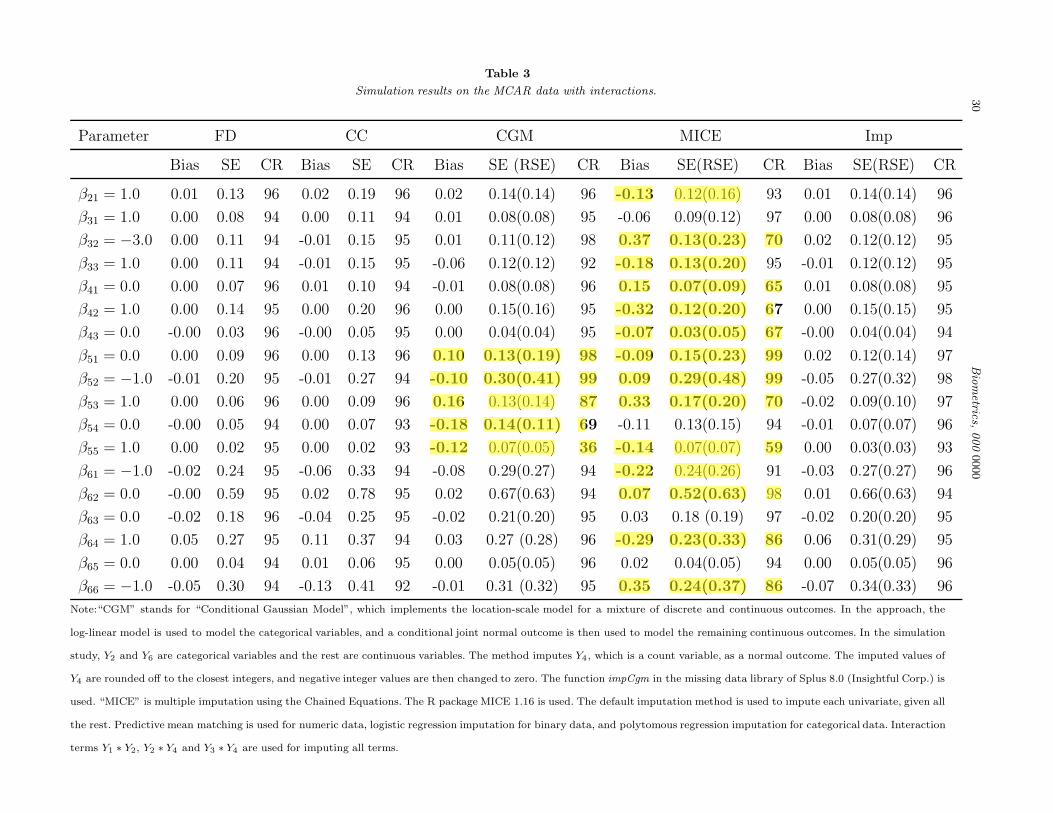
Table 3

Simulation results on the MCAR data with interactions.

Parameter FD CC CGM MICE Imp

Bias SE CR Bias SE CR Bias SE (RSE) CR Bias SE(RSE) CR Bias SE(RSE) CR

β21 = 1.0 0.01 0.13 96 0.02 0.19 96 0.02 0.14(0.14) 96 -0.13 0.12(0.16) 93 0.01 0.14(0.14) 96

β31 = 1.0 0.00 0.08 94 0.00 0.11 94 0.01 0.08(0.08) 95 -0.06 0.09(0.12) 97 0.00 0.08(0.08) 96

β32 = −3.0 0.00 0.11 94 -0.01 0.15 95 0.01 0.11(0.12) 98 0.37 0.13(0.23) 70 0.02 0.12(0.12) 95

β33 = 1.0 0.00 0.11 94 -0.01 0.15 95 -0.06 0.12(0.12) 92 -0.18 0.13(0.20) 95 -0.01 0.12(0.12) 95

β41 = 0.0 0.00 0.07 96 0.01 0.10 94 -0.01 0.08(0.08) 96 0.15 0.07(0.09) 65 0.01 0.08(0.08) 95

β42 = 1.0 0.00 0.14 95 0.00 0.20 96 0.00 0.15(0.16) 95 -0.32 0.12(0.20) 67 0.00 0.15(0.15) 95

β43 = 0.0 -0.00 0.03 96 -0.00 0.05 95 0.00 0.04(0.04) 95 -0.07 0.03(0.05) 67 -0.00 0.04(0.04) 94

β51 = 0.0 0.00 0.09 96 0.00 0.13 96 0.10 0.13(0.19) 98 -0.09 0.15(0.23) 99 0.02 0.12(0.14) 97

β52 = −1.0 -0.01 0.20 95 -0.01 0.27 94 -0.10 0.30(0.41) 99 0.09 0.29(0.48) 99 -0.05 0.27(0.32) 98

β53 = 1.0 0.00 0.06 96 0.00 0.09 96 0.16 0.13(0.14) 87 0.33 0.17(0.20) 70 -0.02 0.09(0.10) 97

β54 = 0.0 -0.00 0.05 94 0.00 0.07 93 -0.18 0.14(0.11) 69 -0.11 0.13(0.15) 94 -0.01 0.07(0.07) 96

β55 = 1.0 0.00 0.02 95 0.00 0.02 93 -0.12 0.07(0.05) 36 -0.14 0.07(0.07) 59 0.00 0.03(0.03) 93

β61 = −1.0 -0.02 0.24 95 -0.06 0.33 94 -0.08 0.29(0.27) 94 -0.22 0.24(0.26) 91 -0.03 0.27(0.27) 96

β62 = 0.0 -0.00 0.59 95 0.02 0.78 95 0.02 0.67(0.63) 94 0.07 0.52(0.63) 98 0.01 0.66(0.63) 94

β63 = 0.0 -0.02 0.18 96 -0.04 0.25 95 -0.02 0.21(0.20) 95 0.03 0.18 (0.19) 97 -0.02 0.20(0.20) 95

β64 = 1.0 0.05 0.27 95 0.11 0.37 94 0.03 0.27 (0.28) 96 -0.29 0.23(0.33) 86 0.06 0.31(0.29) 95

β65 = 0.0 0.00 0.04 94 0.01 0.06 95 0.00 0.05(0.05) 96 0.02 0.04(0.05) 94 0.00 0.05(0.05) 96

β66 = −1.0 -0.05 0.30 94 -0.13 0.41 92 -0.01 0.31 (0.32) 95 0.35 0.24(0.37) 86 -0.07 0.34(0.33) 96

Note:“CGM” stands for “Conditional Gaussian Model”, which implements the location-scale model for a mixture of discrete and continuous outcomes. In the approach, the

log-linear model is used to model the categorical variables, and a conditional joint normal outcome is then used to model the remaining continuous outcomes. In the simulation

study, Y2 and Y6 are categorical variables and the rest are continuous variables. The method imputes Y4 , which is a count variable, as a normal outcome. The imputed values of

Y4 are rounded off to the closest integers, and negative integer values are then changed to zero. The function impCgm in the missing data library of Splus 8.0 (Insightful Corp.) is

used. “MICE” is multiple imputation using the Chained Equations. The R package MICE 1.16 is used. The default imputation method is used to impute each univariate, given all

the rest. Predictive mean matching is used for numeric data, logistic regression imputation for binary data, and polytomous regression imputation for categorical data. Interaction

terms Y1 ∗ Y2, Y2 ∗ Y4 and Y3 ∗ Y4 are used for imputing all terms.

Imputa

tion

Thro

ugh

Odds

Ratio

Mod

els31

Table 4

Simulation results for the MAR data with interactions.

Parameter FD CC CGM MICE Imp

Bias SE CR Bias SE CR Bias SE (RSE) CR Bias SE(RSE) CR Bias SE(RSE) CR

β21 = 1.0 0.02 0.13 95 0.80 0.35 34 0.02 0.14(0.13) 95 0.02 0.13(0.13) 95 0.02 0.13(0.13) 95

β31 = 1.0 0.00 0.08 94 -0.16 0.12 73 0.00 0.08(0.08) 96 0.00 0.08(0.08) 94 0.00 0.08(0.08) 94

β32 = −3.0 0.01 0.11 96 0.15 0.17 84 0.01 0.11(0.11) 94 0.01 0.11(0.11) 96 0.01 0.11(0.11) 96

β33 = 1.0 0.00 0.11 94 -0.03 0.17 95 0.00 0.11(0.11) 96 0.00 0.12(0.11) 94 0.00 0.12(0.11) 94

β41 = 0.0 0.00 0.07 94 0.01 0.10 96 -0.00 0.08(0.08) 95 0.02 0.09(0.09) 94 0.00 0.08(0.08) 96

β42 = 1.0 0.00 0.14 97 0.00 0.18 94 -0.02 0.15(0.15) 95 -0.08 0.16(0.16) 93 0.00 0.14(0.15) 95

β43 = 0.0 -0.00 0.03 94 -0.00 0.05 96 -0.00 0.04(0.04) 96 0.04 0.04(0.04) 86 0.01 0.04(0.04) 94

β51 = 0.0 -0.00 0.09 93 -0.00 0.13 94 0.00 0.15(0.23) 99 -0.08 0.22(0.33) 99 0.00 0.12(0.14) 98

β52 = −1.0 0.01 0.20 93 0.01 0.26 93 -0.23 0.31(0.47) 97 -1.07 0.53(0.68) 72 -0.01 0.26(0.29) 97

β53 = 1.0 0.00 0.06 95 0.00 0.09 96 0.45 0.14(0.19) 26 1.13 0.32(0.35) 5 0.03 0.11(0.12) 96

β54 = 0.0 -0.00 0.05 95 -0.00 0.06 94 -0.06 0.10(0.11) 95 0.15 0.13(0.18) 90 -0.01 0.07(0.08) 96

β55 = 1.0 0.00 0.02 94 0.00 0.03 95 -0.23 0.06(0.07) 2 -0.44 0.13(0.18) 15 -0.02 0.07(0.05) 90

β61 = −1.0 -0.01 0.23 95 -0.03 0.32 95 -0.15 0.27(0.26) 91 -0.01 0.27(0.27) 94 -0.02 0.27(0.27) 94

β62 = 0.0 -0.00 0.55 96 -0.01 0.73 96 0.11 0.65(0.63) 94 -0.11 0.56(0.61) 97 -0.00 0.63(0.63) 95

β63 = 0.0 -0.00 0.17 94 -0.00 0.26 96 -0.04 0.21(0.21) 94 -0.00 0.20(0.21) 97 0.00 0.22(0.21) 95

β64 = 1.0 0.04 0.25 94 0.05 0.32 97 0.04 0.29(0.30) 97 0.02 0.30(0.30) 96 0.05 0.30(0.30) 96

β65 = 0.0 -0.00 0.04 95 -0.00 0.07 95 -0.01 0.06(0.05) 93 -0.00 0.05(0.05) 98 -0.00 0.06(0.05) 95

β66 = −1.0 -0.05 0.28 95 -0.05 0.37 97 -0.06 0.33(0.34) 96 0.01 0.30 (0.33) 97 -0.05 0.34(0.34) 96

See Table 3 for definitions of abbreviations.

A Simulation Study

When no interaction exists, all MI methods: MI using SOR, theJoint normal and Sequential imputation method (MICE) performreasonably well and better than CC.

JN and sequential imputation method can perform poorly inaccommodating interactions. JN cannot model interactionterms and the conditional models used in the sequentialimputation are in conflict with each other.

SOR provides a robust and flexible alternative to the existingMI softwares.

Multiple Imputation by OR model – p. 31/35

Application: Bone Fracture Data

A case-control study of risk factors of hip fracture among maleveterans (Barengolts et al. 2001)

Nine Risk factors considered in this study.

All risk factors are subject to missing values.

Only 237 out of 436 subjects have complete data.

MI runs 2000 iteration for burn-in period.

After burn-in period, generate 20 imputed datasets for every150 iterations.

A logistic model for hip fracture outcome was used to analyzeimputed datasets and the results are pooled using Rubin’scombination rule.

Multiple Imputation by OR model – p. 32/35

Application: Bone Fracture DataTable 1: Analysis of the imputed bone fracture data

Method

Variable CC MICE CGM IMPA IMPB

Etoh 1.39(0.39) 1.23(0.31) 1.18(0.30) 1.24(0.31) 1.30(0.34)

Smoke 0.93(0.40) 0.62(0.30) 0.51(0.29) 0.67(0.32) 0.64(0.32)

Dementia 2.51(0.72) 1.61(0.47) 1.54(0.45) 1.56(0.46) 1.58(0.45)

Antiseiz 3.31(1.06) 2.51(0.64) 2.44(0.60) 2.56(0.62) 2.56(0.62)

LevoT4 2.01(1.02) 0.92(0.64) 0.88(0.55) 0.97(0.62) 0.85(0.60)

AntiChol -1.92(0.77) -1.49(0.59) -0.91(0.48) -1.62(0.55) -1.56(0.56)

Albumin -0.91(0.35) -1.03(0.28) -1.01(0.26) -1.01(0.30) -0.90(0.29)

BMI -0.10(0.04) -0.10(0.03) -0.11(0.03) -0.10(0.03) -0.10(0.03)

log(HGB) -2.60(1.20) -3.39(0.93) -3.18(0.88) -3.20(0.96) -3.38(0.99)

Multiple Imputation by OR model – p. 33/35

Application: Bone Fracture DataTable 2: Analysis of the imputed bone fracture data

Method

Variable CC MICE CGM IMPA IMPB

Etoh 1.41(0.40) 1.13(0.29) 1.15(0.30) 1.27(0.31) 1.31(0.30)

Smoke -9.21(5.69) -5.32(4.34) -3.05(4.52) -2.97(4.54) -3.14(4.63)

Dementia 2.80(0.79) 1.69(0.47) 1.54(0.47) 1.60(0.48) 1.63(0.47)

Antiseiz 4.12(1.29) 2.45(0.62) 2.51(0.63) 2.67(0.66) 2.76(0.65)

LevoT4 3.15(1.34) 0.41(0.65) 1.03(0.63) 1.00(0.66) 0.89(0.62)

AntiChol 5.08(4.15) -0.72(1.99) -1.26(2.34) -2.87(2.29) -3.32(2.20)

Albumin 5.90(4.04) -3.07(3.40) 2.53(2.97) 2.80(3.02) 2.60(3.40)

BMI -0.12(0.04) -0.12(0.03) -0.11(0.03) -0.11(0.03) -0.10(0.03)

log(HGB) 4.60(5.99) -7.56(4.80) 1.02(4.35) 1.46(4.43)) 1.26(4.76)

smoke*loghgb 4.05(2.28) 2.40(1.74) 1.40(1.79) 1.82(1.80) 1.64(1.84)

AntiChol*albumin -2.36(1.40) 0.02(0.55) 0.07(0.62) 0.36(0.65) 0.50 (0.63)

Albumin*loghgb -2.67(1.67) 0.95(1.35) -1.43(1.19) -1.58(1.22) -1.52 (1.36)

Multiple Imputation by OR model – p. 34/35

Discussion

We proposed a new MI approach based on semiparametricodds ratio model.

The approach is more flexible than existing methods

Unlike the joint model, higher order terms can be incorporatedinto model.

Unlike sequential imputation model, the SOR approach iscompatible.

Can accommodate different shapes of distributions.

Imputation model is more general than GLM, commonly usedfor data analysis.

More research is needed for model selection for nonlinearterms in the model.

Multiple Imputation by OR model – p. 35/35