multivariate data analysis (mva) - introduction · problems with univariate methods for...
TRANSCRIPT
10/9/2012 MVA intro 2008 H. Antti 1
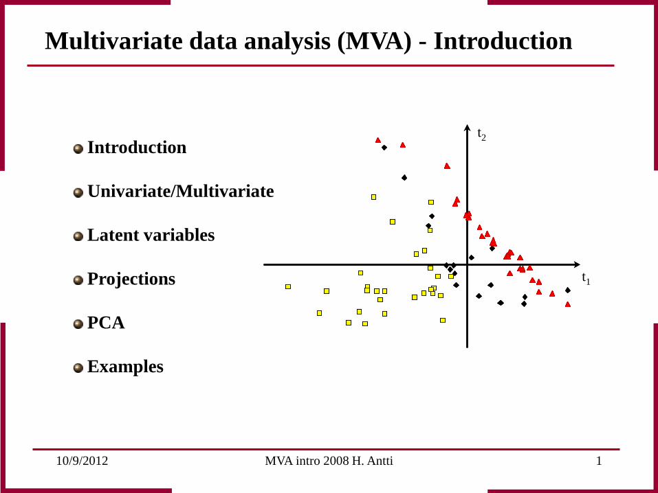
Multivariate data analysis (MVA) - Introduction
Introduction
Univariate/Multivariate
Latent variables
Projections
PCA
Examples
t1
t2
10/9/2012 MVA intro 2008 H. Antti 2
K
N
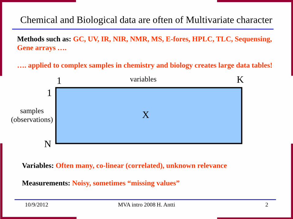
Chemical and Biological data are often of Multivariate character
samples (observations)
1 1 variables
Methods such as: GC, UV, IR, NIR, NMR, MS, E-fores, HPLC, TLC, Sequensing, Gene arrays …. …. applied to complex samples in chemistry and biology creates large data tables!
Variables: Often many, co-linear (correlated), unknown relevance Measurements: Noisy, sometimes “missing values”
X
10/9/2012 MVA intro 2008 H. Antti 3
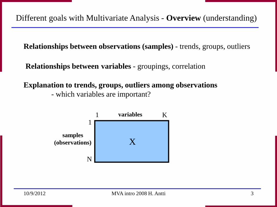
Different goals with Multivariate Analysis - Overview (understanding)
Relationships between observations (samples) - trends, groups, outliers Relationships between variables - groupings, correlation Explanation to trends, groups, outliers among observations - which variables are important?
K
N
samples (observations)
1 1 variables
X
10/9/2012 MVA intro 2008 H. Antti 4
K
N
samples (observations)
1 1 variables
I II III
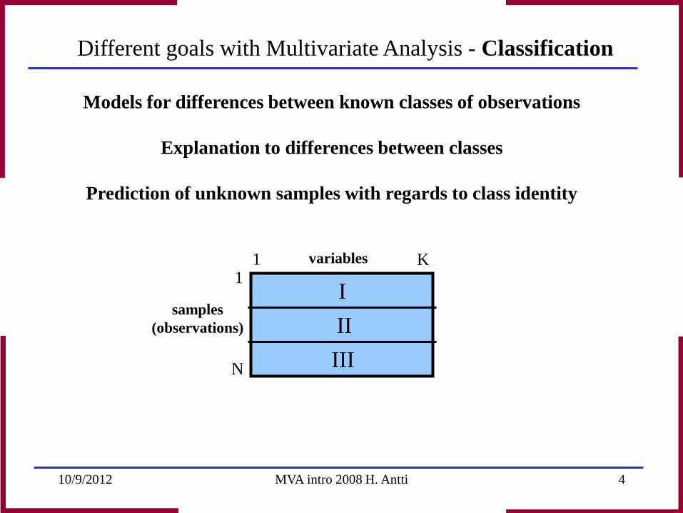
Models for differences between known classes of observations
Explanation to differences between classes
Prediction of unknown samples with regards to class identity
Different goals with Multivariate Analysis - Classification
10/9/2012 MVA intro 2008 H. Antti 5
K
N
samples (observations)
1 1 variables
X Y
1 M
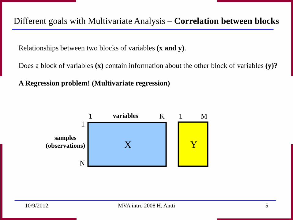
Relationships between two blocks of variables (x and y). Does a block of variables (x) contain information about the other block of variables (y)? A Regression problem! (Multivariate regression)
Different goals with Multivariate Analysis – Correlation between blocks
10/9/2012 MVA intro 2008 H. Antti 6
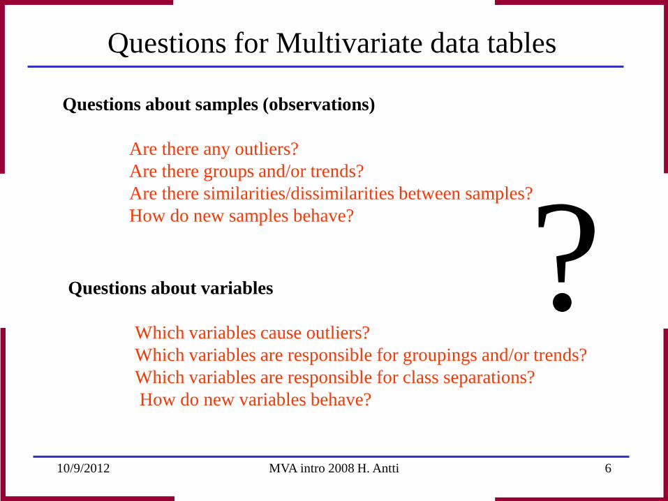
Questions for Multivariate data tables
Questions about samples (observations) Are there any outliers? Are there groups and/or trends? Are there similarities/dissimilarities between samples? How do new samples behave?
Questions about variables Which variables cause outliers? Which variables are responsible for groupings and/or trends? Which variables are responsible for class separations? How do new variables behave?
?
10/9/2012 MVA intro 2008 H. Antti 7
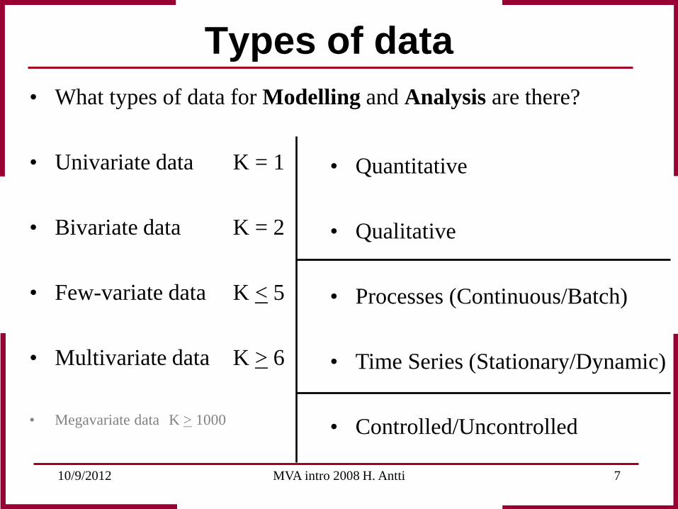
Types of data • What types of data for Modelling and Analysis are there?
• Univariate data K = 1
• Bivariate data K = 2
• Few-variate data K < 5
• Multivariate data K > 6
• Megavariate data K > 1000
• Quantitative
• Qualitative
• Processes (Continuous/Batch)
• Time Series (Stationary/Dynamic)
• Controlled/Uncontrolled
10/9/2012 MVA intro 2008 H. Antti 8
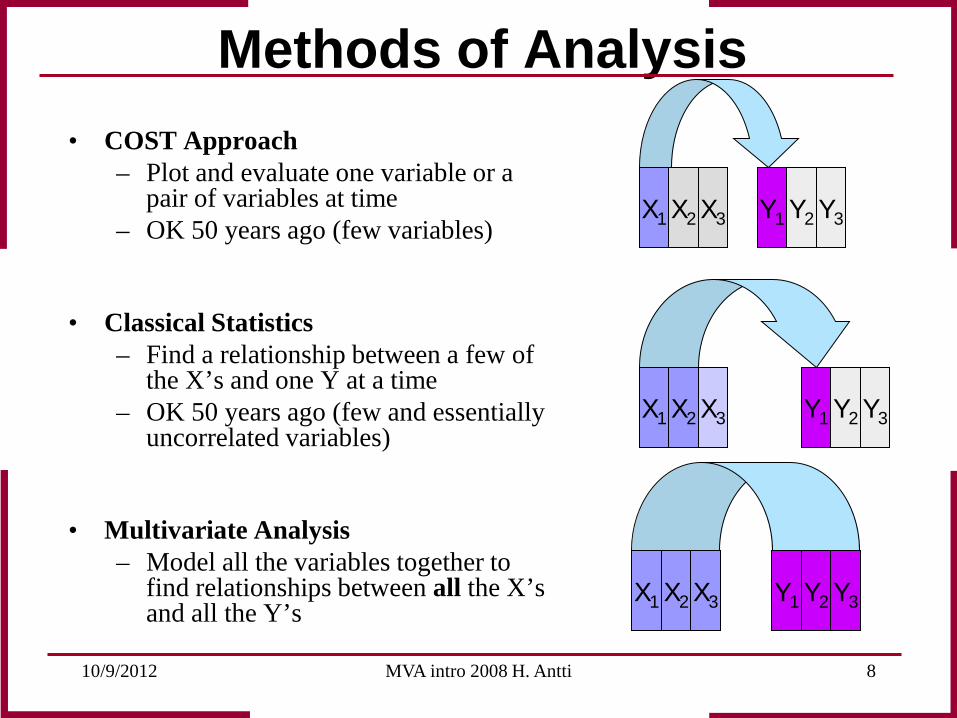
Methods of Analysis
X1 Y1 Y2 Y3 X2 X3
X1 Y1 Y2 Y3 X2 X3
X1 Y1 Y2 Y3 X2 X3
• COST Approach – Plot and evaluate one variable or a
pair of variables at time – OK 50 years ago (few variables)
• Classical Statistics – Find a relationship between a few of
the X’s and one Y at a time – OK 50 years ago (few and essentially
uncorrelated variables)
• Multivariate Analysis – Model all the variables together to
find relationships between all the X’s and all the Y’s
10/9/2012 MVA intro 2008 H. Antti 9
Problems with univariate methods for Multivariate data
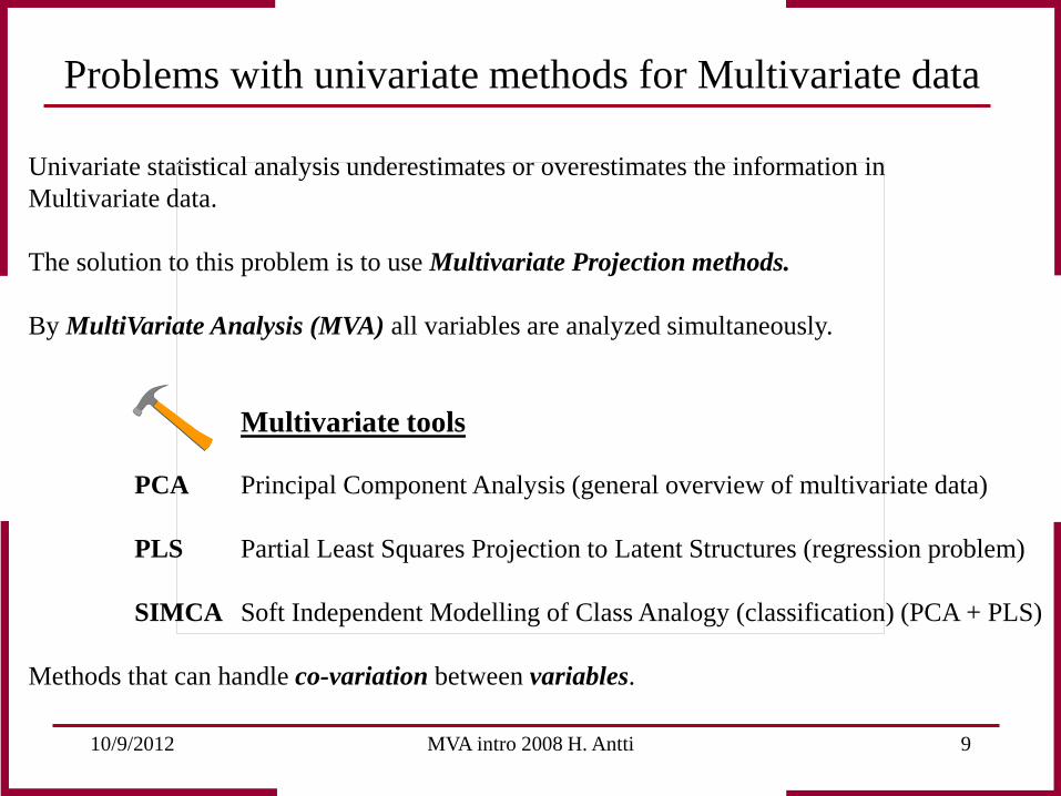
Univariate statistical analysis underestimates or overestimates the information in Multivariate data. The solution to this problem is to use Multivariate Projection methods. By MultiVariate Analysis (MVA) all variables are analyzed simultaneously. PCA Principal Component Analysis (general overview of multivariate data) PLS Partial Least Squares Projection to Latent Structures (regression problem) SIMCA Soft Independent Modelling of Class Analogy (classification) (PCA + PLS) Methods that can handle co-variation between variables.
This image cannot currently be displayed.
Multivariate tools
10/9/2012 MVA intro 2008 H. Antti 10
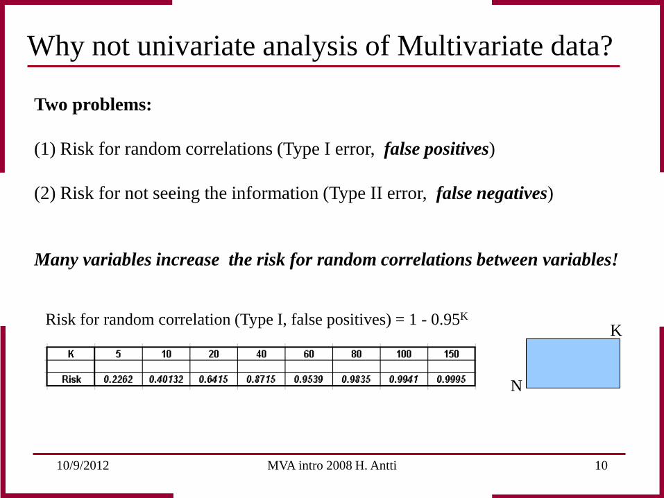
Why not univariate analysis of Multivariate data? Two problems: (1) Risk for random correlations (Type I error, false positives) (2) Risk for not seeing the information (Type II error, false negatives) Many variables increase the risk for random correlations between variables!
N
K Risk for random correlation (Type I, false positives) = 1 - 0.95K
10/9/2012 MVA intro 2008 H. Antti 11
# of
che
eseb
urge
rs
blood-lipidsfa
ith in
God
salary ofswedish priests
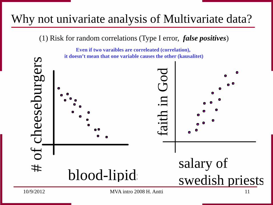
(1) Risk for random correlations (Type I error, false positives) Even if two varaibles are correleated (correlation),
it doesn’t mean that one variable causes the other (kausalitet)
Why not univariate analysis of Multivariate data?
10/9/2012 MVA intro 2008 H. Antti 12
-4 -3 -2 -1 0 1 2 3 4 -4
-3
-2
-1
0
1
2
3
4
2 Outliers!!!
Var
iabl
e 1
Variable 2 10 20 30 40
-4
-3
-2
-1
0
1
2
3
4
-3 Sd
+3 Sd
Var
iabl
e 1
Time
-4 -3 -2 -1 0 1 2 3 4 40
30
20
10
-3 S
d
+3 S
d
Tim
e
Variable 2
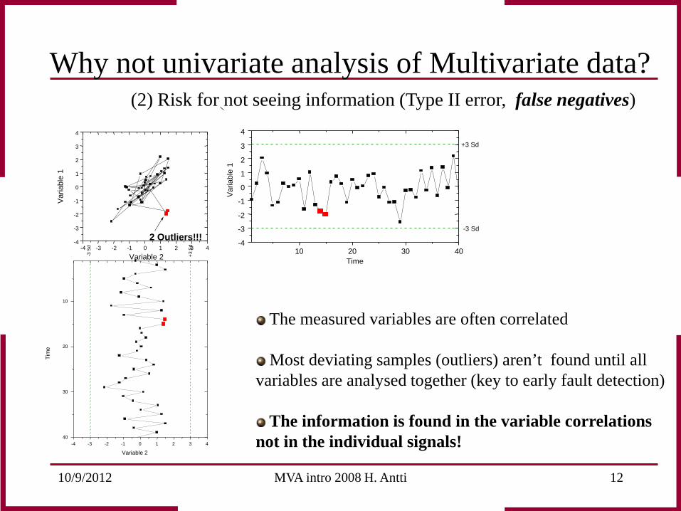
The measured variables are often correlated Most deviating samples (outliers) aren’t found until all
variables are analysed together (key to early fault detection) The information is found in the variable correlations
not in the individual signals!
(2) Risk for not seeing information (Type II error, false negatives)
Why not univariate analysis of Multivariate data?
10/9/2012 MVA intro 2008 H. Antti 13
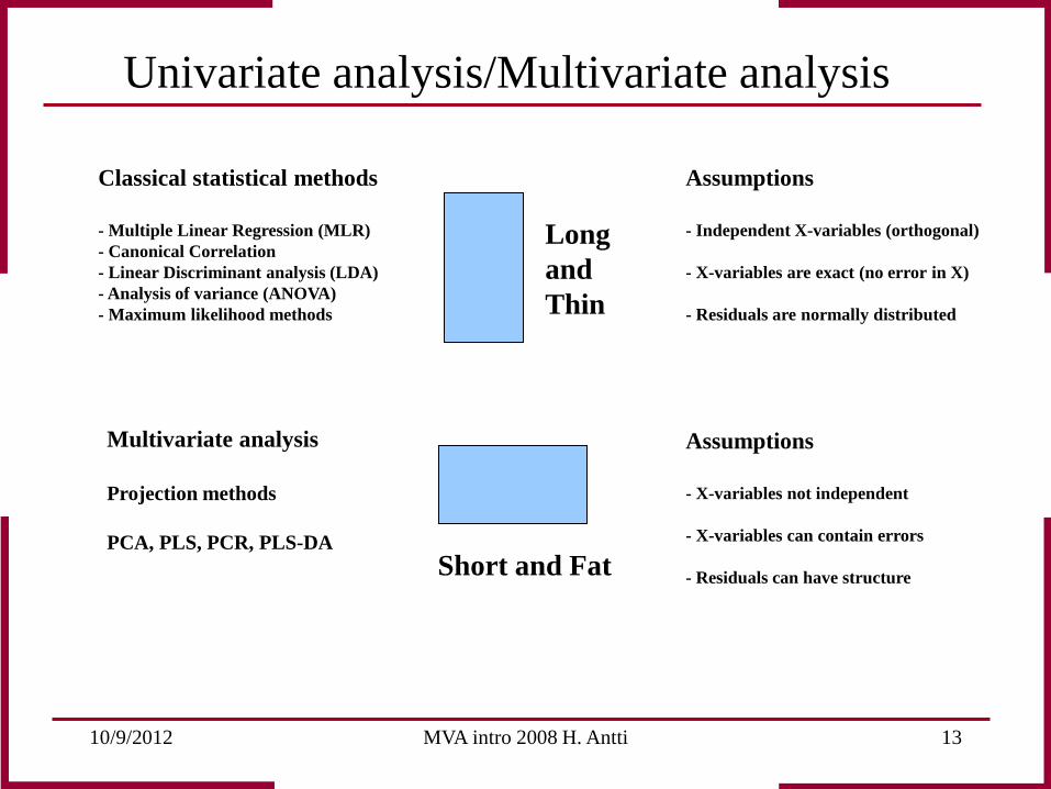
Long and Thin
Short and Fat
Classical statistical methods - Multiple Linear Regression (MLR) - Canonical Correlation - Linear Discriminant analysis (LDA) - Analysis of variance (ANOVA) - Maximum likelihood methods
Multivariate analysis Projection methods PCA, PLS, PCR, PLS-DA
Assumptions - Independent X-variables (orthogonal) - X-variables are exact (no error in X) - Residuals are normally distributed
Assumptions - X-variables not independent - X-variables can contain errors - Residuals can have structure
Univariate analysis/Multivariate analysis
10/9/2012 MVA intro 2008 H. Antti 14
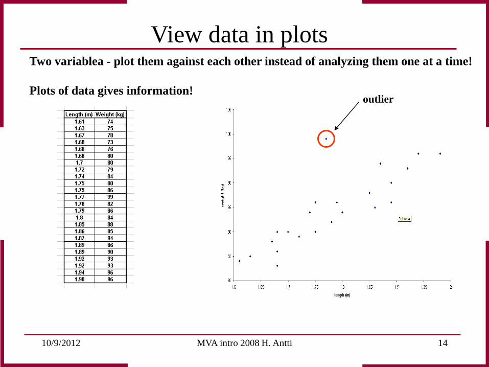
outlier
View data in plots Two variablea - plot them against each other instead of analyzing them one at a time! Plots of data gives information!
10/9/2012 MVA intro 2008 H. Antti 15
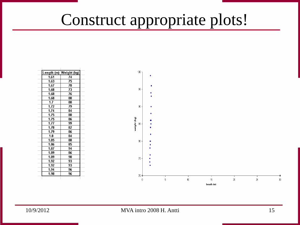
Construct appropriate plots!
10/9/2012 MVA intro 2008 H. Antti 16
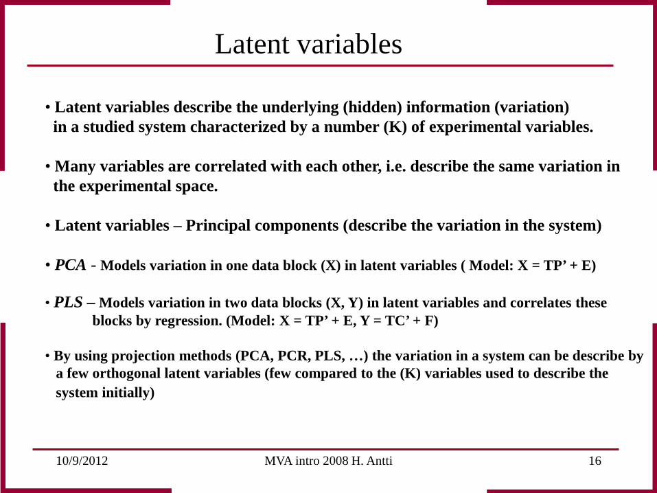
Latent variables
• Latent variables describe the underlying (hidden) information (variation) in a studied system characterized by a number (K) of experimental variables. • Many variables are correlated with each other, i.e. describe the same variation in the experimental space. • Latent variables – Principal components (describe the variation in the system) • PCA - Models variation in one data block (X) in latent variables ( Model: X = TP’ + E) • PLS – Models variation in two data blocks (X, Y) in latent variables and correlates these blocks by regression. (Model: X = TP’ + E, Y = TC’ + F) • By using projection methods (PCA, PCR, PLS, …) the variation in a system can be describe by a few orthogonal latent variables (few compared to the (K) variables used to describe the system initially)

10/9/2012 MVA intro 2008 H. Antti 17
Latent variables (PCA)
N
K t1 t2... ta
p’a p’2 p’1
P’ T
ti: score vector pi: loading vector T: matrix consisting of score vectors (N*A) P: matrix consisting of loading vectors (K*A) X
• A principal component (latent variable) consists of two parts (score (ti) + loading (pi)) • Scores (t) describe the variation in the sample direction i.e. differences/similarities between samples • Loadings (p) describe the variation in the variable direction i.e. differences/similarities between variables and additionally give an explanation to the variation in scores. • The principal components are orthogonal to each other and explain the variation in X that is based on a number (K) of often correlated variables. • The number of principal components (A) is often a lot less than the number of variables (K) in X.
Model
Residual
10/9/2012 MVA intro 2008 H. Antti 18
PC1 (t1p1’)
X
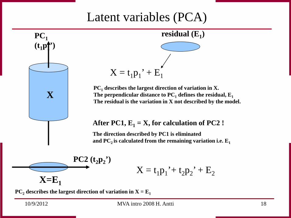
X = t1p1’ + E1
residual (E1)
PC2 (t2p2’) X = t1p1’+ t2p2’ + E2
After PC1, E1 = X, for calculation of PC2 !
PC1 describes the largest direction of variation in X. The perpendicular distance to PC1 defines the residual, E1 The residual is the variation in X not described by the model.
X=E1
The direction described by PC1 is eliminated and PC2 is calculated from the remaining variation i.e. E1
PC2 describes the largest direction of variation in X = E1
Latent variables (PCA)
10/9/2012 MVA intro 2008 H. Antti 19
var. 3
var. 1
var. 2
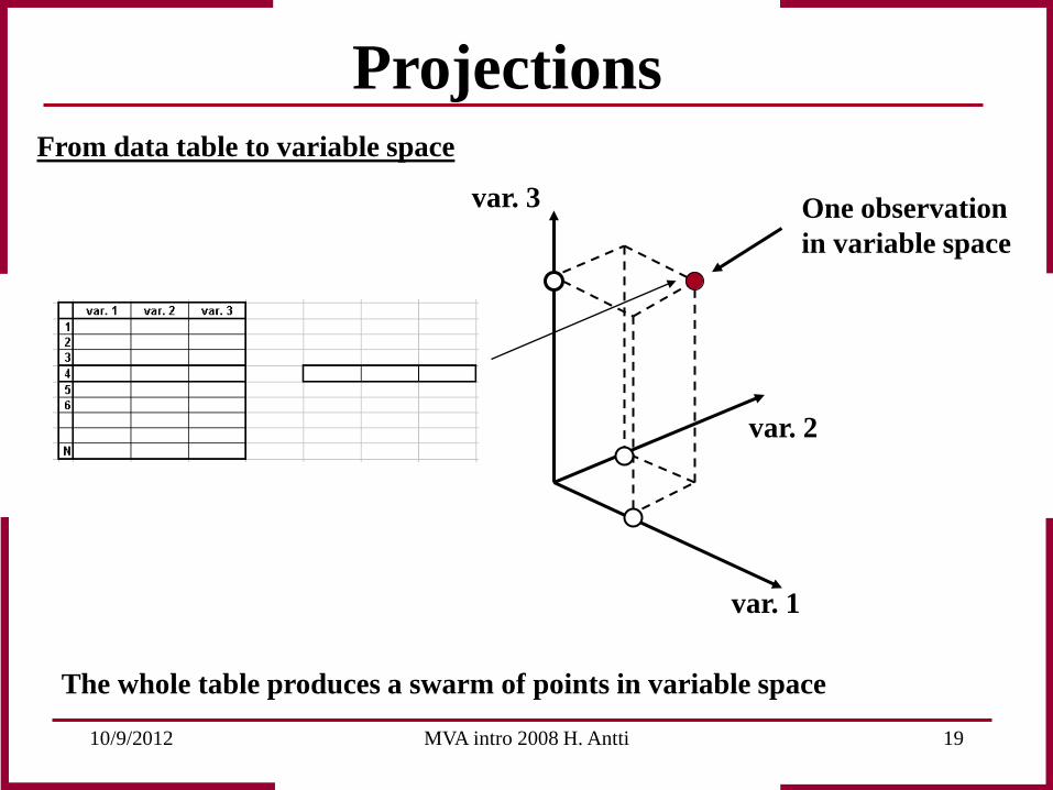
One observation in variable space
From data table to variable space
The whole table produces a swarm of points in variable space
Projections
10/9/2012 MVA intro 2008 H. Antti 20
var. 1
var. 2
var. 3
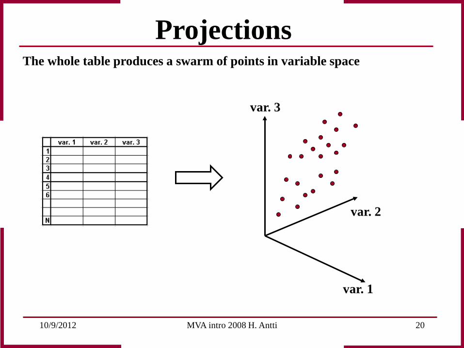
Projections The whole table produces a swarm of points in variable space
10/9/2012 MVA intro 2008 H. Antti 21
var. 1
var. 2
var. 3
average
var. 1
var. 2
var. 3
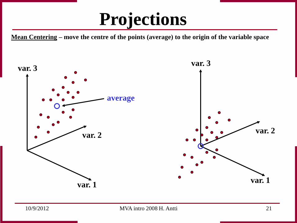
Mean Centering – move the centre of the points (average) to the origin of the variable space
Projections
10/9/2012 MVA intro 2008 H. Antti 22
var. 1
var. 2
var. 3
(i)
ti1
PC1 (t1p’1)
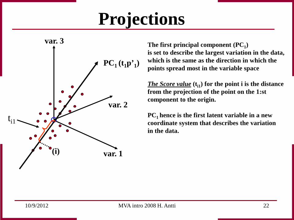
Projections The first principal component (PC1) is set to describe the largest variation in the data, which is the same as the direction in which the points spread most in the variable space The Score value (ti1) for the point i is the distance from the projection of the point on the 1:st component to the origin. PC1 hence is the first latent variable in a new coordinate system that describes the variation in the data.
10/9/2012 MVA intro 2008 H. Antti 23
var. 1
var. 2
var. 3
PC1
PC2
(i)
ti1 ti2
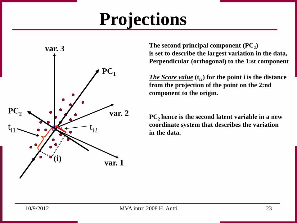
Projections The second principal component (PC2) is set to describe the largest variation in the data, Perpendicular (orthogonal) to the 1:st component The Score value (ti2) for the point i is the distance from the projection of the point on the 2:nd component to the origin. PC2 hence is the second latent variable in a new coordinate system that describes the variation in the data.
10/9/2012 MVA intro 2008 H. Antti 24
var. 1
var. 2
(i) ti1
θ1 θ2
PC1 p = cos θ
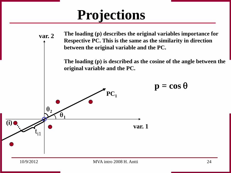
Projections The loading (p) describes the original variables importance for Respective PC. This is the same as the similarity in direction between the original variable and the PC. The loading (p) is described as the cosine of the angle between the original variable and the PC.
10/9/2012 MVA intro 2008 H. Antti 25
var. 1
var. 2
θ2= 90º PC1
θ1= 0º
Projections
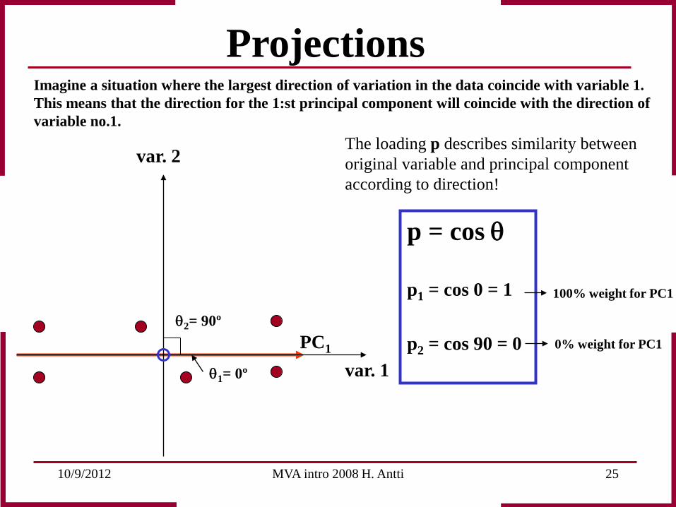
p = cos θ p1 = cos 0 = 1 p2 = cos 90 = 0
Imagine a situation where the largest direction of variation in the data coincide with variable 1. This means that the direction for the 1:st principal component will coincide with the direction of variable no.1.
The loading p describes similarity between original variable and principal component according to direction!
100% weight for PC1
0% weight for PC1
10/9/2012 MVA intro 2008 H. Antti 26
var. 1
var. 2
(i)
PC1
ei
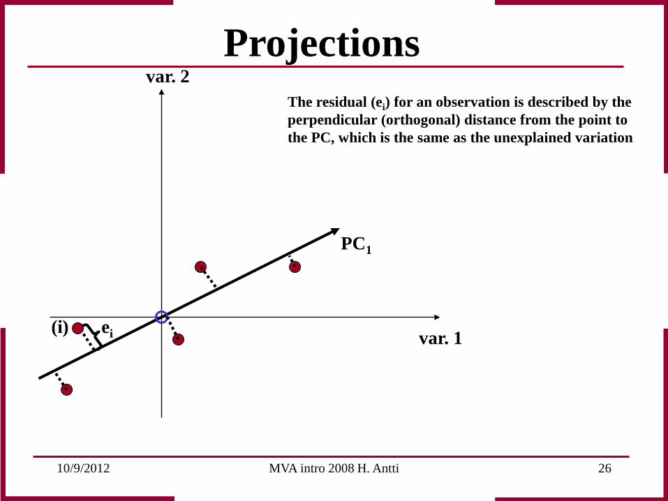
Projections The residual (ei) for an observation is described by the perpendicular (orthogonal) distance from the point to the PC, which is the same as the unexplained variation
10/9/2012 MVA intro 2008 H. Antti 27
var. 1
var. 2
(i)
PC1
ei θ1
θ2
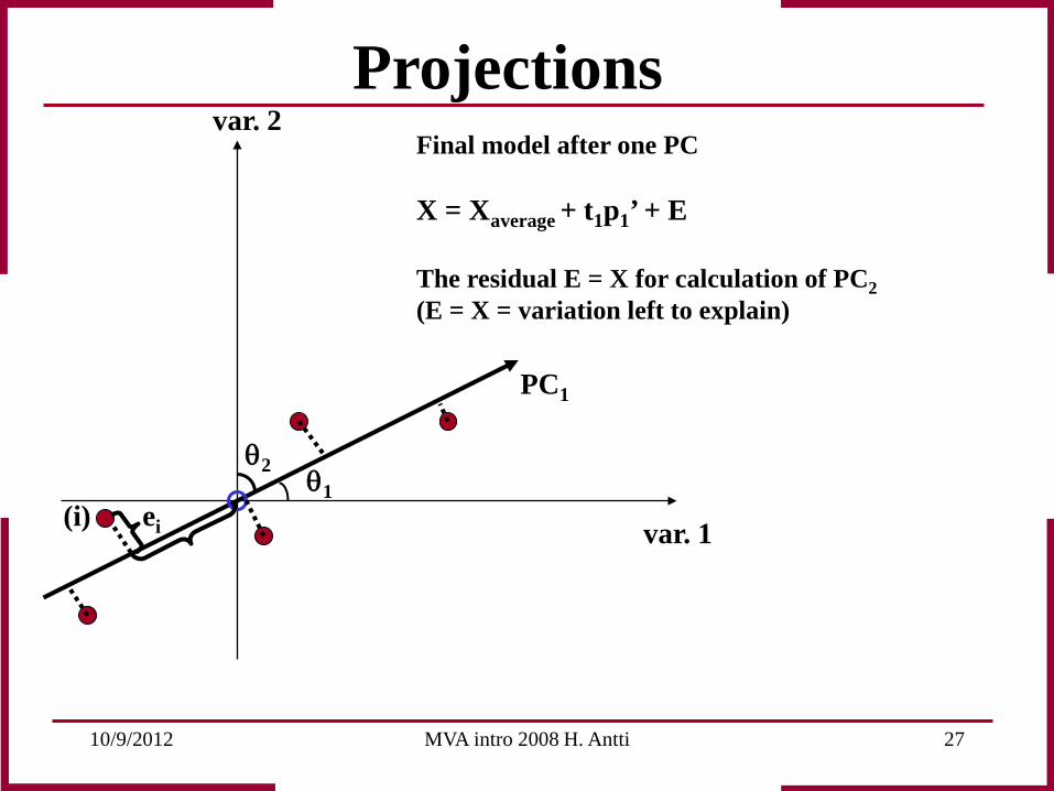
Projections Final model after one PC X = Xaverage + t1p1’ + E The residual E = X for calculation of PC2 (E = X = variation left to explain)
10/9/2012 MVA intro 2008 H. Antti 28
x 1
x 2
x 3
PC 1
PC2
Projection
Plane
observation i
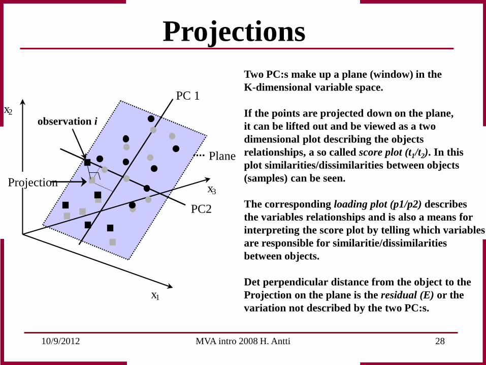
Projections Two PC:s make up a plane (window) in the K-dimensional variable space. If the points are projected down on the plane, it can be lifted out and be viewed as a two dimensional plot describing the objects relationships, a so called score plot (t1/t2). In this plot similarities/dissimilarities between objects (samples) can be seen. The corresponding loading plot (p1/p2) describes the variables relationships and is also a means for interpreting the score plot by telling which variables are responsible for similaritie/dissimilarities between objects. Det perpendicular distance from the object to the Projection on the plane is the residual (E) or the variation not described by the two PC:s.
10/9/2012 MVA intro 2008 H. Antti 29
t1
t2
p1
p2 var.1
var.2
var.3
“scores”
“loadings”
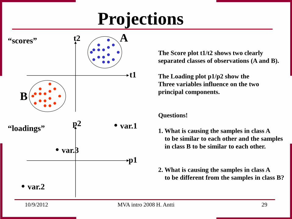
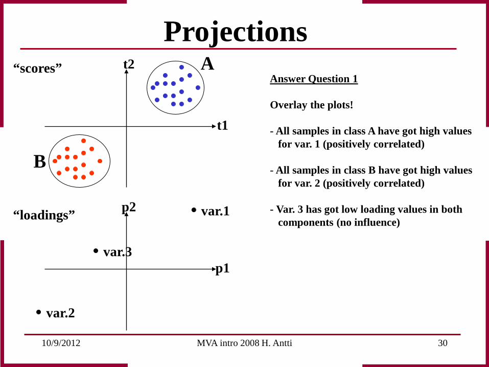
The Score plot t1/t2 shows two clearly separated classes of observations (A and B). The Loading plot p1/p2 show the Three variables influence on the two principal components. Questions! 1. What is causing the samples in class A to be similar to each other and the samples in class B to be similar to each other. 2. What is causing the samples in class A to be different from the samples in class B?
A
B
Projections
10/9/2012 MVA intro 2008 H. Antti 30
t1
t2
p1
p2 var.1
var.2
var.3
“scores”
“loadings”
A
B
Answer Question 1 Overlay the plots! - All samples in class A have got high values for var. 1 (positively correlated) - All samples in class B have got high values for var. 2 (positively correlated) - Var. 3 has got low loading values in both components (no influence)
Projections
10/9/2012 MVA intro 2008 H. Antti 31
t1
t2
p1
p2 var.1
var.2
var.3
“scores”
“loadings”
B
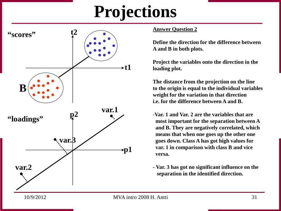
Answer Question 2 Define the direction for the difference between A and B in both plots. Project the variables onto the direction in the loading plot. The distance from the projection on the line to the origin is equal to the individual variables weight for the variation in that direction i.e. for the difference between A and B. -Var. 1 and Var. 2 are the variables that are most important for the separation between A and B. They are negatively correlated, which means that when one goes up the other one goes down. Class A has got high values for var. 1 in comparison with class B and vice versa. - Var. 3 has got no significant influence on the separation in the identified direction.
Projections
10/9/2012 MVA intro 2008 H. Antti 32
x 1
x 2
x 3
PC 1
PC2
Projection
Plane
observation i
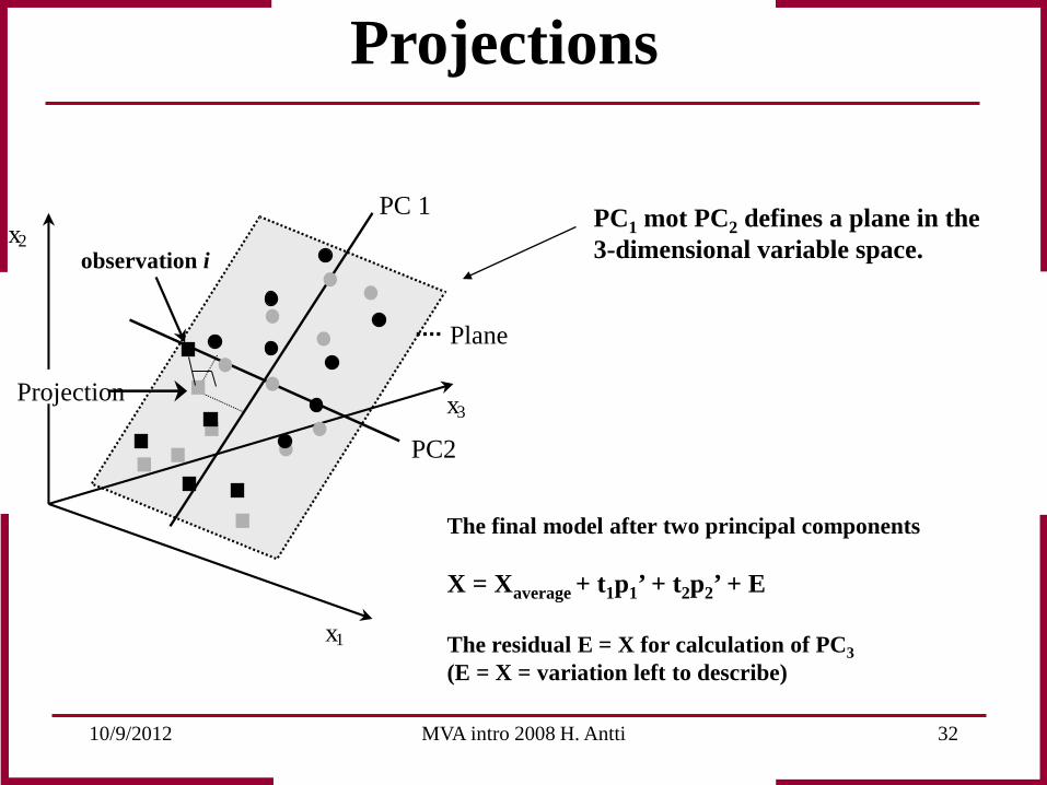
The final model after two principal components X = Xaverage + t1p1’ + t2p2’ + E The residual E = X for calculation of PC3 (E = X = variation left to describe)
PC1 mot PC2 defines a plane in the 3-dimensional variable space.
Projections
10/9/2012 MVA intro 2008 H. Antti 33
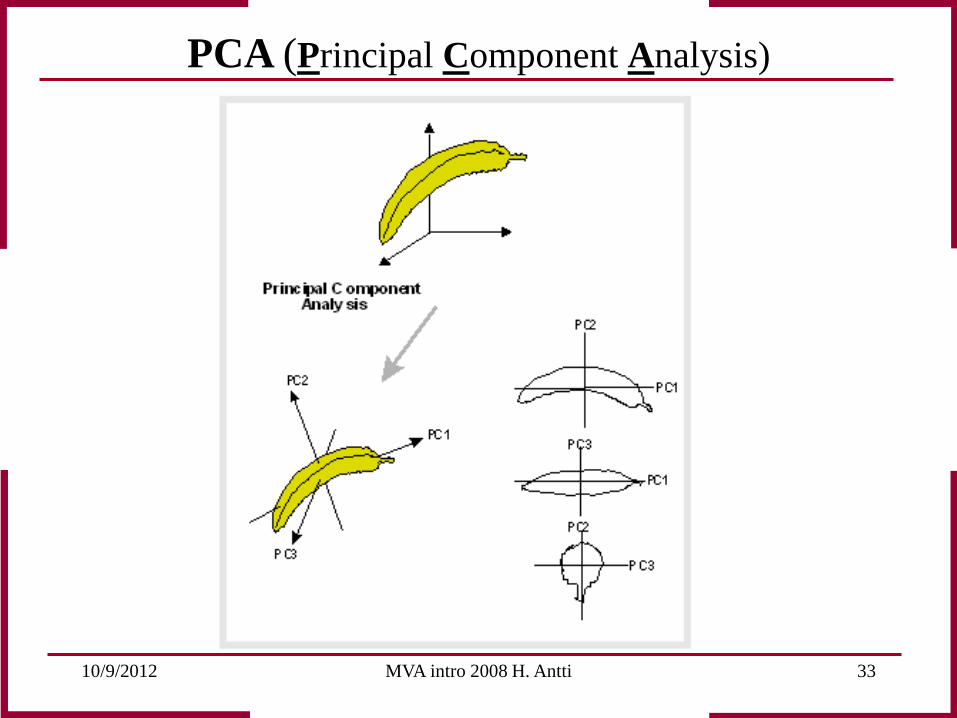
PCA (Principal Component Analysis)
10/9/2012 MVA intro 2008 H. Antti 34
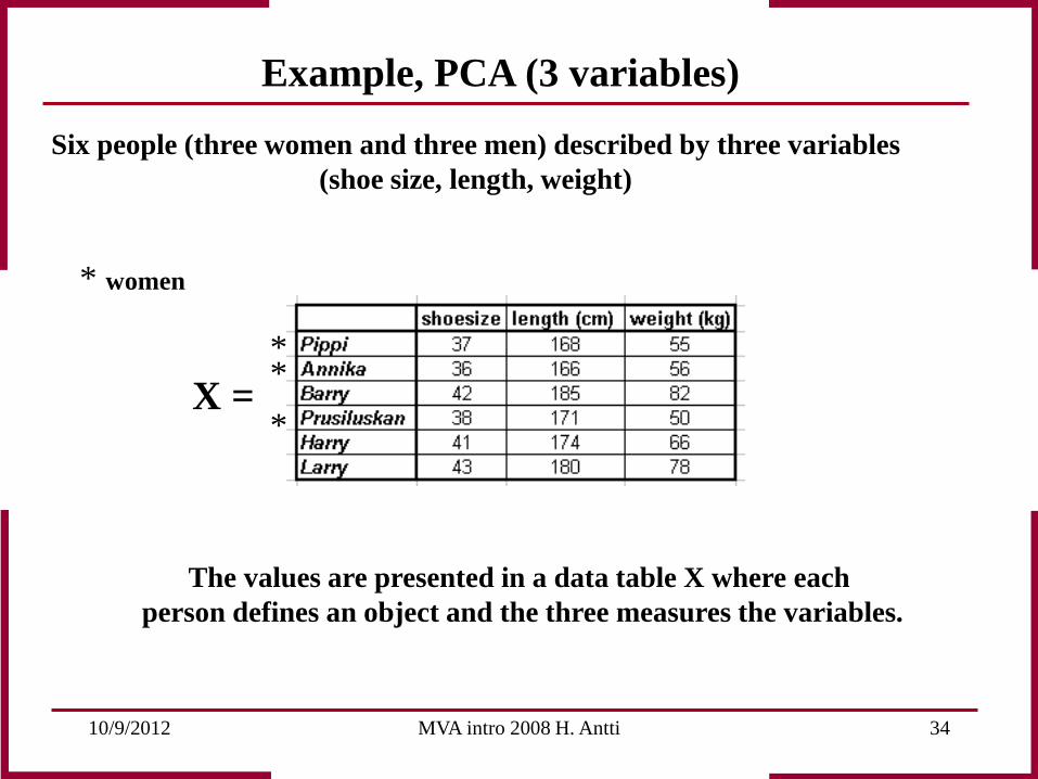
Example, PCA (3 variables)
Six people (three women and three men) described by three variables (shoe size, length, weight)
The values are presented in a data table X where each person defines an object and the three measures the variables.
X =
* women
* * *
10/9/2012 MVA intro 2008 H. Antti 35
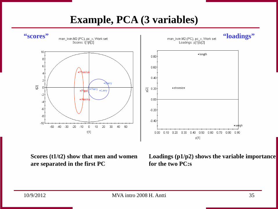
Scores (t1/t2) show that men and women are separated in the first PC
Loadings (p1/p2) shows the variable importance for the two PC:s
Example, PCA (3 variables) “loadings” “scores”

10/9/2012 MVA intro 2008 H. Antti 36
pshoe
plength
pweight
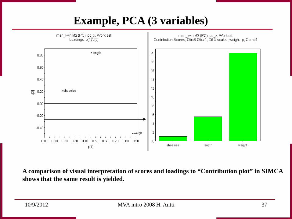
Interpretation of scores and loadings together tell us that the difference between men and women, in this case, is that the men are heavier, are longer and also have bigger feet. The variable importance (weight) for the separation in PC 1 can be viewed in the loading plot. Variable weights for the separation in PC 1: weight > length > shoe size
Example, PCA (3 variables)
10/9/2012 MVA intro 2008 H. Antti 37
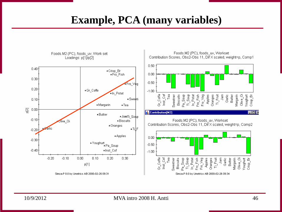
A comparison of visual interpretation of scores and loadings to “Contribution plot” in SIMCA shows that the same result is yielded.
Example, PCA (3 variables)
10/9/2012 MVA intro 2008 H. Antti 38
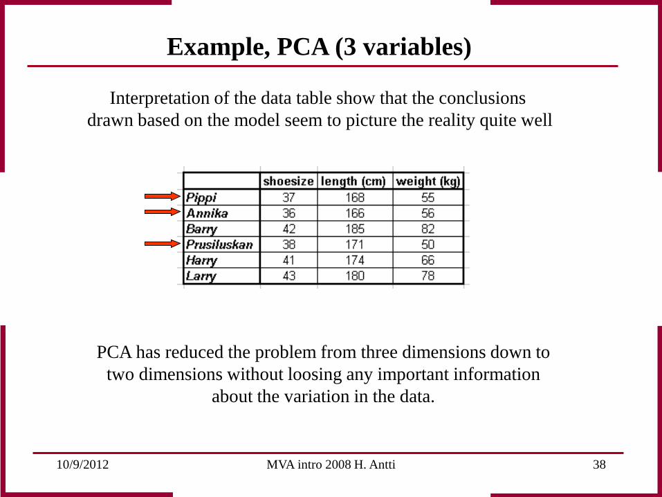
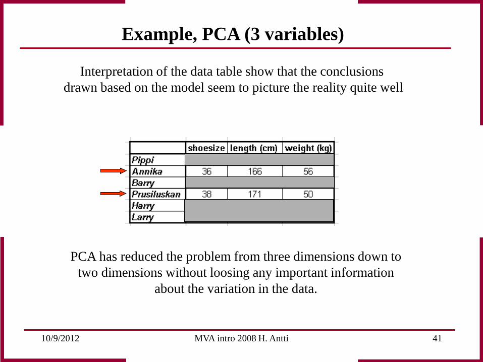
Interpretation of the data table show that the conclusions drawn based on the model seem to picture the reality quite well
PCA has reduced the problem from three dimensions down to two dimensions without loosing any important information
about the variation in the data.
Example, PCA (3 variables)
10/9/2012 MVA intro 2008 H. Antti 39
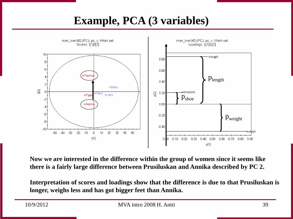
pshoe
plength
pweight
Now we are interested in the difference within the group of women since it seems like there is a fairly large difference between Prusiluskan and Annika described by PC 2. Interpretation of scores and loadings show that the difference is due to that Prusiluskan is longer, weighs less and has got bigger feet than Annika.
Example, PCA (3 variables)
10/9/2012 MVA intro 2008 H. Antti 40
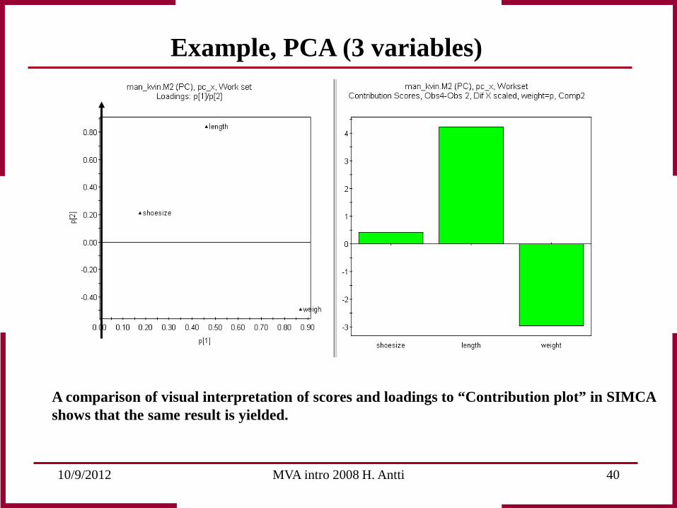
Example, PCA (3 variables)
A comparison of visual interpretation of scores and loadings to “Contribution plot” in SIMCA shows that the same result is yielded.
10/9/2012 MVA intro 2008 H. Antti 41
Interpretation of the data table show that the conclusions drawn based on the model seem to picture the reality quite well
PCA has reduced the problem from three dimensions down to two dimensions without loosing any important information
about the variation in the data.
Example, PCA (3 variables)
10/9/2012 MVA intro 2008 H. Antti 42
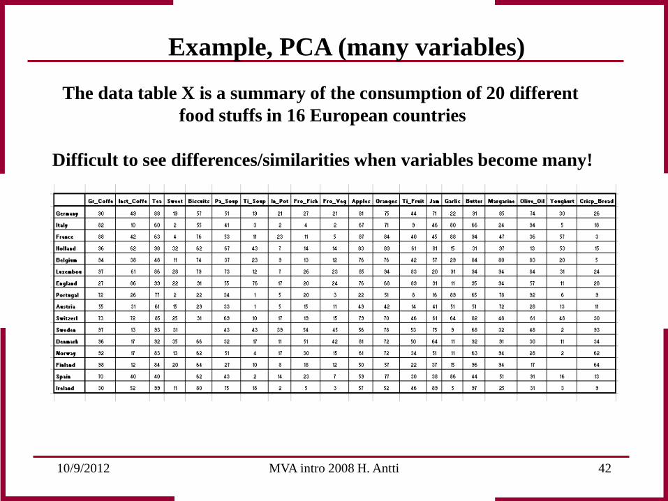
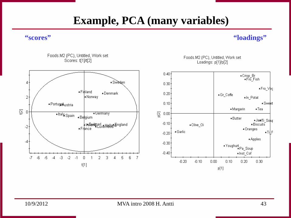
Example, PCA (many variables)
The data table X is a summary of the consumption of 20 different food stuffs in 16 European countries
Difficult to see differences/similarities when variables become many!
10/9/2012 MVA intro 2008 H. Antti 43
“scores” “loadings”
Example, PCA (many variables)
10/9/2012 MVA intro 2008 H. Antti 44
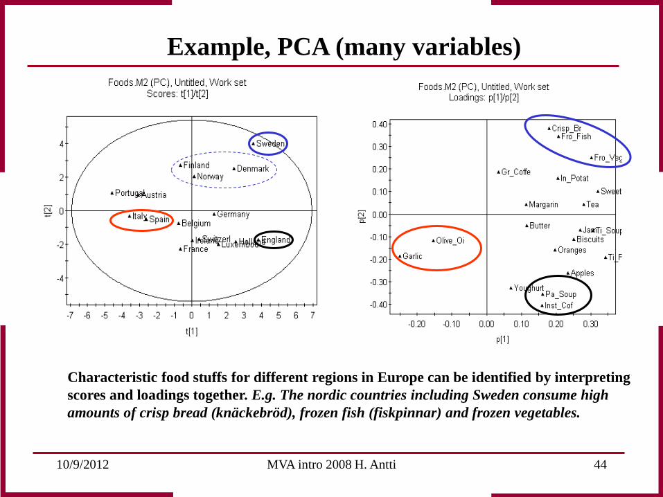
Characteristic food stuffs for different regions in Europe can be identified by interpreting scores and loadings together. E.g. The nordic countries including Sweden consume high amounts of crisp bread (knäckebröd), frozen fish (fiskpinnar) and frozen vegetables.
Example, PCA (many variables)
10/9/2012 MVA intro 2008 H. Antti 45
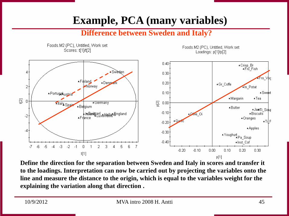
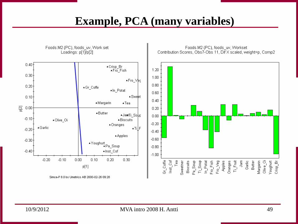
Example, PCA (many variables) Difference between Sweden and Italy?
Define the direction for the separation between Sweden and Italy in scores and transfer it to the loadings. Interpretation can now be carried out by projecting the variables onto the line and measure the distance to the origin, which is equal to the variables weight for the explaining the variation along that direction .
10/9/2012 MVA intro 2008 H. Antti 46
Example, PCA (many variables)
10/9/2012 MVA intro 2008 H. Antti 47
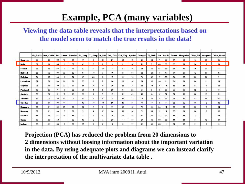
Viewing the data table reveals that the interpretations based on the model seem to match the true results in the data!
Projection (PCA) has reduced the problem from 20 dimensions to 2 dimensions without loosing information about the important variation in the data. By using adequate plots and diagrams we can instead clarify the interpretation of the multivariate data table .
Example, PCA (many variables)

10/9/2012 MVA intro 2008 H. Antti 48
Example, PCA (many variables) Difference between Sweden and England?
Define the direction for the separation between Sweden and England in scores and transfer it to the loadings. Interpretation can now be carried out by projecting the variables onto the line and measure the distance to the origin, which is equal to the variables weight for the explaining the variation along that direction .
10/9/2012 MVA intro 2008 H. Antti 49
Example, PCA (many variables)
10/9/2012 MVA intro 2008 H. Antti 50
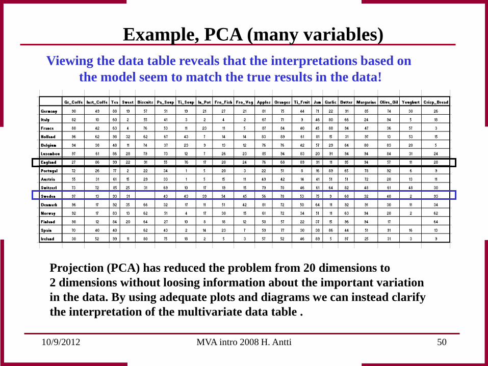
Viewing the data table reveals that the interpretations based on the model seem to match the true results in the data!
Projection (PCA) has reduced the problem from 20 dimensions to 2 dimensions without loosing information about the important variation in the data. By using adequate plots and diagrams we can instead clarify the interpretation of the multivariate data table .
Example, PCA (many variables)
10/9/2012 MVA intro 2008 H. Antti 51
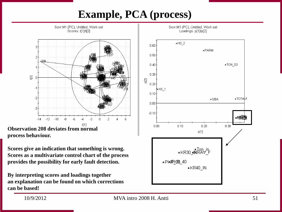
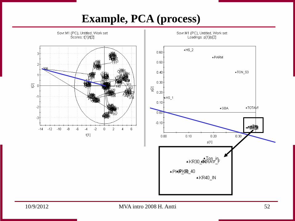
Example, PCA (process)
Observation 208 deviates from normal process behaviour. Scores give an indication that something is wrong. Scores as a multivariate control chart of the process provides the possibility for early fault detection. By interpreting scores and loadings together an explanation can be found on which corrections can be based!
10/9/2012 MVA intro 2008 H. Antti 52
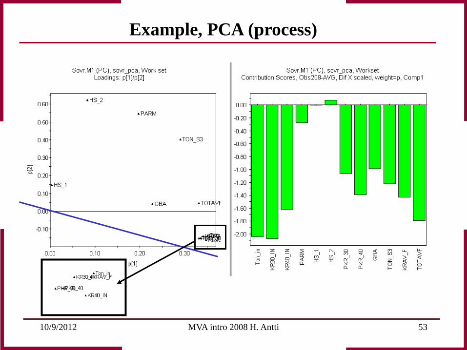
Example, PCA (process)
10/9/2012 MVA intro 2008 H. Antti 53
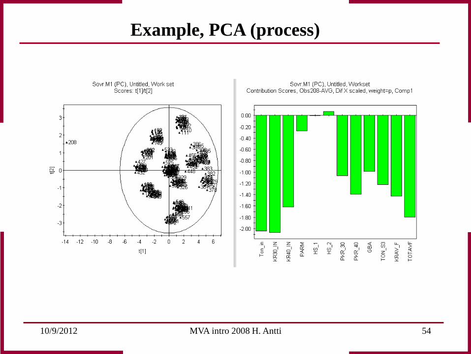
Example, PCA (process)
10/9/2012 MVA intro 2008 H. Antti 54
Example, PCA (process)
10/9/2012 MVA intro 2008 H. Antti 55
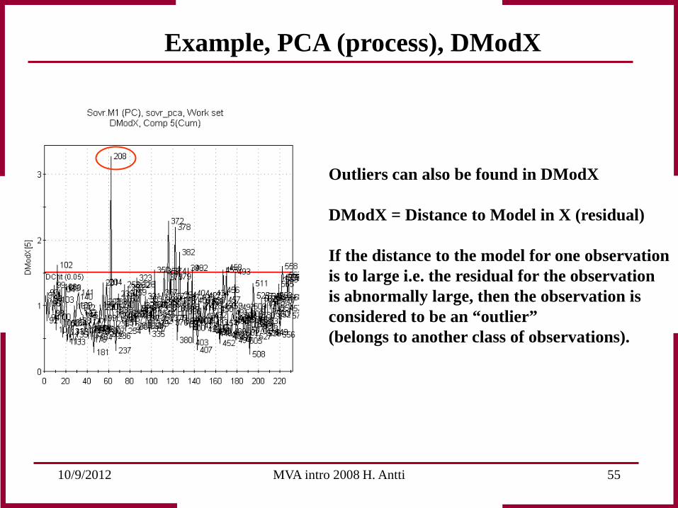
Example, PCA (process), DModX
Outliers can also be found in DModX DModX = Distance to Model in X (residual) If the distance to the model for one observation is to large i.e. the residual for the observation is abnormally large, then the observation is considered to be an “outlier” (belongs to another class of observations).
10/9/2012 MVA intro 2008 H. Antti 56
var. 1
var. 2
(i)
PC1
ei
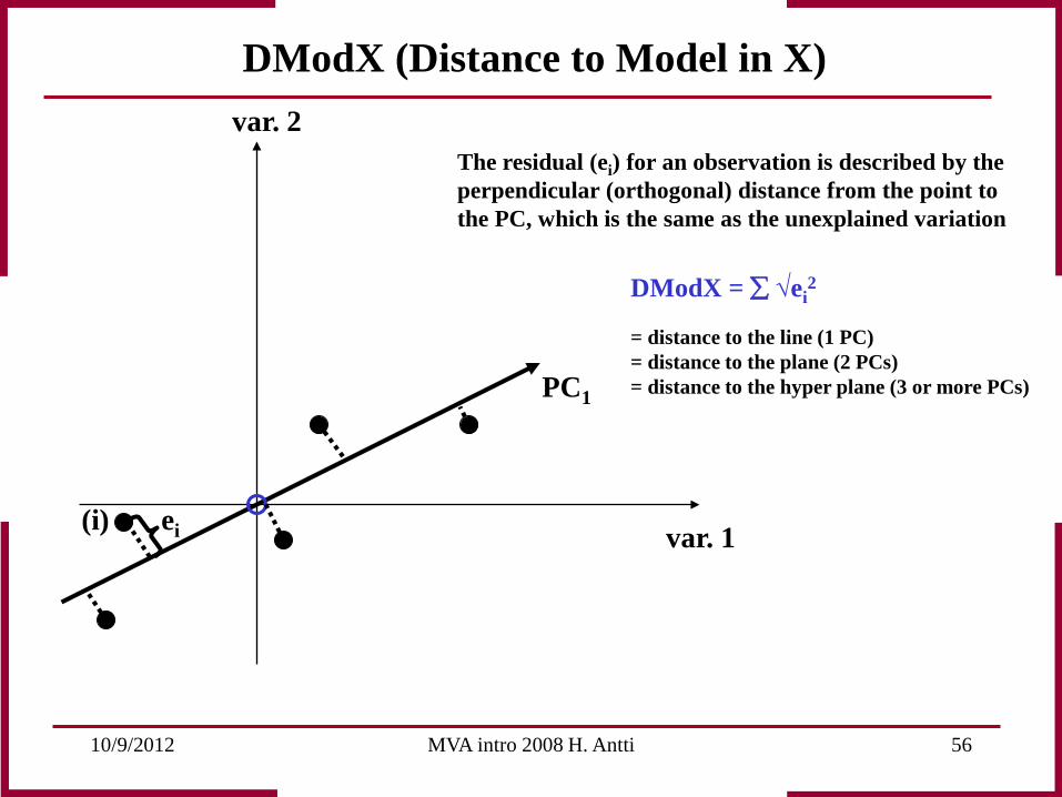
DModX (Distance to Model in X)
DModX = ∑ √ei2
= distance to the line (1 PC) = distance to the plane (2 PCs) = distance to the hyper plane (3 or more PCs)
The residual (ei) for an observation is described by the perpendicular (orthogonal) distance from the point to the PC, which is the same as the unexplained variation
10/9/2012 MVA intro 2008 H. Antti 57
No. Name F.W. m.p. nd density b.p. f.p. pka Mol V Spec ref Mol ref clogP logP No. C No. H No. N No. O Rings1 2-Amino-5-diethylaminopentane 158.29 1.4429 0.817 68 193.75 0.542 85.81 0.955 9 22 2 0 02 2-Amino-3,3-dimethylbutane 101.19 -20 1.413 0.755 102.5 134.03 0.547 55.35 1.501 6 15 1 0 03 2-Aminoheptane 115.22 1.4175 0.766 143 54 10.88 150.42 0.545 62.80 2.29 2.4 7 17 1 0 04 tert -Amylamine 87.17 1.3996 0.746 77 -1 116.85 0.536 46.69 1.102 5 13 1 0 05 n-Butylamine 73.14 -49 1.4010 0.740 78 -14 10.65 98.838 0.542 39.634 0.923 0.97 4 11 1 0 06 (R)-(-)-sec -Butylamine 73.14 1.3936 0.720 63 -19 10.61 101.58 0.547 39.98 0.703 0.74 4 11 1 0 07 (S)-(+)-sec-Butylamine 73.14 62 1.3930 0.731 62.5 -19 10.61 100.05 0.538 39.32 0.703 0.74 4 11 1 0 08 tert -Butylamine 73.14 -67 1.3780 0.696 46 -8 10.69 105.09 0.543 39.72 0.573 4 4 11 1 0 09 Decylamine 157.3 13 1.436 0.787 217 85 10.64 199.87 0.554 87.14 4.097 10 23 1 0 010 1,3-Dimethylbutylamine 101.19 1.4085 0.717 109 12 141.13 0.570 57.65 1.631 6 15 1 0 011 3,3-Dimethylbutylamine 101.19 1.4135 0.752 115 5 134.56 0.550 55.64 1.721 6 15 1 0 012 1,5-Dimethylhexylamine 129.25 1.4215 0.767 155 48 10.38 168.51 0.550 71.03 2.689 8 19 1 0 013 (±)-1,2-Dimethylpropylamine 87.17 -50 1.4055 0.757 85.5 -27 115.15 0.536 46.69 1.102 5 13 1 0 014 Dodecylamine 185.36 31 0.806 248 10.67 229.98 5.155 12 27 1 0 015 Ethylamine 45.09 -81 1.3663 0.689 16.6 -16 10.81 65.44 0.532 23.97 -0.135 -0.13 2 7 1 0 016 2-Ethylbutylamine 101.194 21.5 1.4209 0.776 125.5 13 130.40 0.542 54.89 1.851 6 15 1 0 017 (±)-2-Ethylhexylamine 129.25 -76 1.43 0.789 169 52 163.81 0.545 70.44 2.909 2.82 8 19 1 0 018 1-Ethylpropylamine 87.17 1.4055 0.748 90 2 10.59 116.54 0.542 47.26 1.232 5 13 1 0 019 Heptylamine 115.22 1.4243 0.777 155 35 10.66 148.29 0.546 62.92 2.51 2.57 7 17 1 0 020 1-Hexadecylamine 241.46 44 330 140 10.61 7.271 16 35 1 0 021 Hexylamine 101.19 -23 1.418 0.766 131.5 8 10.56 132.10 0.546 55.22 1.981 2.06 6 15 1 0 022 Isoamylamine 87.17 1.4089 0.751 96 18 10.6 116.07 0.544 47.46 1.322 6 13 1 0 023 Isobutylamine 73.14 -85 1.397 0.736 67.5 -20 10.42 99.38 0.539 39.45 0.793 0.73 4 11 1 0 024 Isopropylamine 59.11 -110 1.3746 0.694 33.5 -32 10.71 85.17 0.540 31.91 0.174 0.26 3 9 1 0 025 Methylamine 31.06 -93 1.08 -6.3/760 0 10.66 28.76 -0.664 -0.57 1 5 1 0 026 1-Methylbutylamine 87.17 1.4029 0.736 91 35 10.65 118.44 0.547 47.72 1.232 5 13 1 0 027 2-Methylbutylamine 87.17 1.4116 0.738 95.5 3 - 118.12 0.558 48.62 1.322 5 13 1 0 028 (S)-(-)-2-Methylbutylamine 87.17 1.4126 0.738 42.5/12 3 - 118.12 0.559 48.73 1.322 5 13 1 0 029 1-Methylheptylamine 129.25 1.4235 0.771 165 50 167.64 0.549 71.00 2.819 8 19 1 0 030 Neopentylamine 87.17 1.403 0.745 81.5/741 -13 9.85 117.01 0.541 47.15 1.192 5 13 1 0 031 Nonylamine 143.27 1.433 0.782 201 62 10.64 183.21 0.554 79.33 3.568 9 21 1 0 032 Octadecylamine 269.52 56 10.6 8.329 18 39 1 0 033 Octylamine 129.25 -3 1.429 0.782 176 62 10.65 165.28 0.549 70.91 3.039 8 19 1 0 034 tert -Octylamine 129.25 1.424 0.805 140 32 10.84 160.56 0.527 68.08 2.429 8 19 1 0 035 Pentadecylamine 227.44 37.5 300 10.61 6.742 15 33 1 0 036 Pentylamine (amylamine) 87.17 -50 1.411 0.752 104 4 10.63 115.92 0.547 47.64 1.452 1.49 5 13 1 0 037 Propylamine 59.11 -83 1.3885 0.719 48 -37 10.71 82.21 0.540 31.94 0.394 0.47 3 9 1 0 038 1-Tetradecylamine 213.41 41 162/15 10.62 6.213 14 31 1 0 039 Tridecylamine 199.38 31 265 11 5.684 13 29 1 0 040 Undecylamine 171.33 16.5 1.4388 0.796 240 92 10.63 215.24 0.551 94.45 4.626 11 25 1 0 041 (R)-(-)-2-Amino-1-butanol 89.14 -2 1.4525 0.947 173 82 94.13 0.478 42.59 0.052 4 11 1 1 042 (±)-2-Amino-1-butanol 89.14 -2 1.4518 0.943 177 84 94.53 0.479 42.71 0.052 4 11 1 1 043 S-(+)-2-Amino-1-butanol 89.14 1.4521 0.944 173 79 94.43 0.479 42.69 0.052 4 11 1 1 044 4-Amino-1-butanol 89.14 1.4610 0.967 206 107 92.18 0.477 42.50 -1.064 4 11 1 1 045 2-(2-Aminoethoxy)ethanol 105.14 1.0480 1.048 221 100.32 0.046 4.82 -1.231 4 11 1 2 046 (±)-2-Amino-3-methyl-1-butanol 103.17 1.4543 0.936 76/8 90 110.22 0.485 50.07 -0.058 5 13 1 1 047 S-(+)-2-Amino-3-methyl-1-butanol 103.17 31 1.4548 0.926 81/8 91 111.41 0.491 50.67 -0.058 5 13 1 1 048 2-Amino-2-methyl-1-propanol 89.14 26 1.4455 0.934 165 67 95.44 0.477 42.52 -0.587 4 11 1 1 049 DL-2-Amino-1-pentanol 103.17 1.4511 0.922 194.5 95 111.90 0.489 50.48 0.072 5 13 1 1 050 5-Amino-1-pentanol 103.17 36 1.4615 0.949 122/16 65 108.71 0.486 50.17 -0.535 5 13 1 1 051 (±)-3-Amino-1,2-propanediol 91.11 1.4920 1.175 264.5/739 77.54 0.419 38.15 -2.12 3 9 1 2 052 R -(-)-1-Amino-2-propanol 75.11 25 1.4482 0.954 160 73 78.73 0.470 35.29 -0.986 -0.96 3 9 1 1 053 DL-1-Amino-2-propanol 75.11 -2 1.4483 0.973 160 73 77.19 0.461 34.61 -0.986 -0.96 3 9 1 1 054 S -(+)-1-Amino-2-propanol 75.11 25 1.4437 0.954 160 76 78.73 0.465 34.93 -0.986 -0.96 3 9 1 1 055 (R )-(-)-2-Amino-1-propanol 75.11 1.4493 0.965 174.5 83 77.83 0.466 34.97 -0.986 3 9 1 1 056 DL-2-Amino-1-propanol 75.11 1.4495 0.943 174.5 83 79.65 0.477 35.80 -0.986 3 9 1 1 057 (S )-(+)-2-Amino-1-propanol 75.11 1.4498 0.965 72.5/11 62 77.83 0.466 35.01 -0.986 3 9 1 1 058 3-Amino-1-propanol 75.11 11 1.4610 0.982 187.5 79 76.49 0.469 35.26 -1.593 -1.12 3 9 1 1 059 Ethanolamine 61.08 10.5 1.454 1.012 170 93 60.36 0.449 27.40 -1.295 -1.31 2 7 1 1 060 (R)-(-)-Leucinol 117.19 1.4496 0.917 199/768 90 127.80 0.490 57.46 -0.388 6 15 1 1 061 4-Aminobutyraldehyde diethyl acetal 161.25 1.4275 0.933 196 62 172.83 0.458 73.88 0.104 8 19 1 2 062 (±)-2-Amino-1-methoxypropane 89.14 1.4065 0.845 93/743 8 105.49 0.481 42.88 -0.363 4 11 1 1 063 3-Butoxypropylamine 131.22 1.4260 0.853 169.5/756 63 153.83 0.499 65.53 1.444 7 17 1 1 064 3-Ethoxypropylamine 103.17 1.4178 0.861 137 32 119.83 0.485 50.06 -0.488 5 13 1 1 065 Ethyl 3-aminobutyrate 131.18 1.4241 0.894 60.5/13 42 146.73 0.474 62.23 0.439 6 13 1 2 066 3-Isopropoxypropylamine 117.19 1.4195 0.845 78.5/85 39 138.69 0.496 58.18 -0.179 6 15 1 1 067 2-Methoxyethylamine 75.11 1.406 0.864 95 9 86.93 0.470 35.29 -0.672 3 9 1 1 068 3-Methoxypropylamine 89.14 1.4175 0.874 117.5/733 22 101.99 0.478 42.58 -1.017 4 11 1 1 069 1-Adamantanemethylamine 165.28 1.5137 0.933 92 177.15 0.551 91.00 3.173 11 19 1 0 370 (Aminomethyl)cyclopropane 71.12 1.4340 0.820 86/758 -30 86.73 0.529 37.64 0.309 4 9 1 0 1
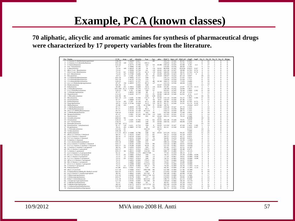
Example, PCA (known classes) 70 aliphatic, alicyclic and aromatic amines for synthesis of pharmaceutical drugs were characterized by 17 property variables from the literature.
10/9/2012 MVA intro 2008 H. Antti 58
aromatic
aliphatic
alicyclic
t 1
t 2
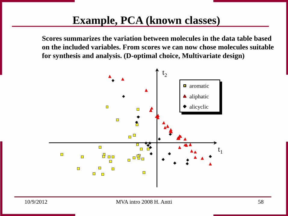
Scores summarizes the variation between molecules in the data table based on the included variables. From scores we can now chose molecules suitable for synthesis and analysis. (D-optimal choice, Multivariate design)
Example, PCA (known classes)
10/9/2012 MVA intro 2008 H. Antti 59
1050
17 X
Example, PCA (spectroscopic data)
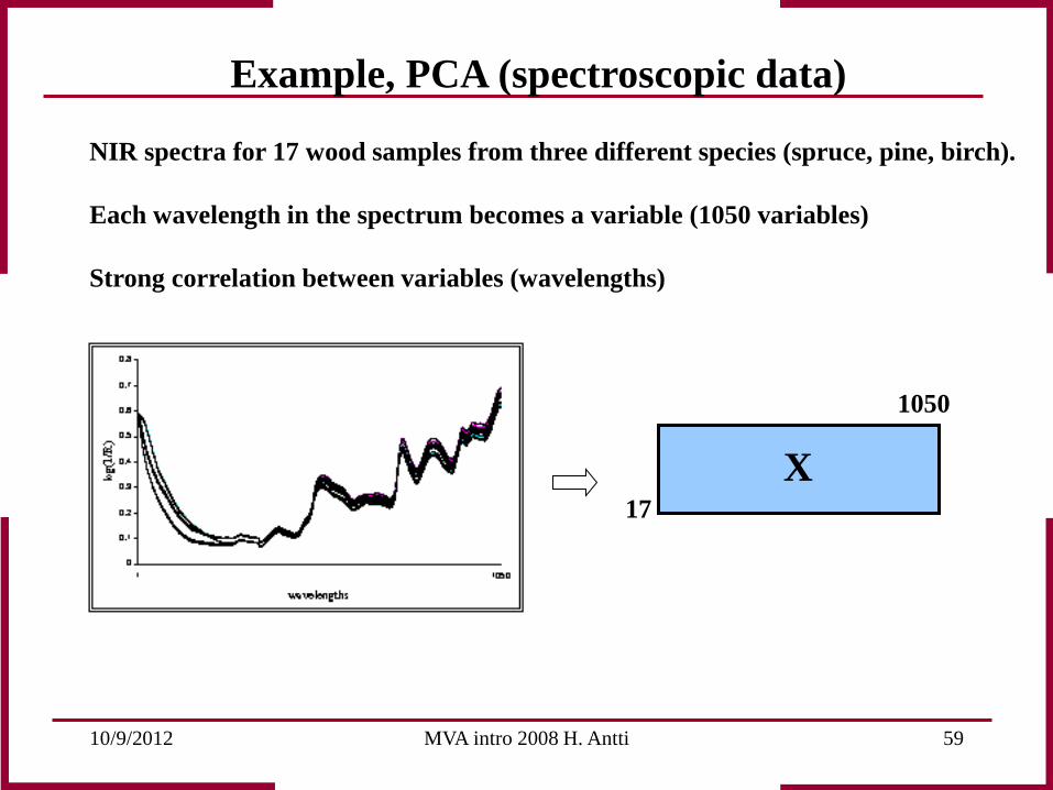
NIR spectra for 17 wood samples from three different species (spruce, pine, birch). Each wavelength in the spectrum becomes a variable (1050 variables) Strong correlation between variables (wavelengths)
10/9/2012 MVA intro 2008 H. Antti 60
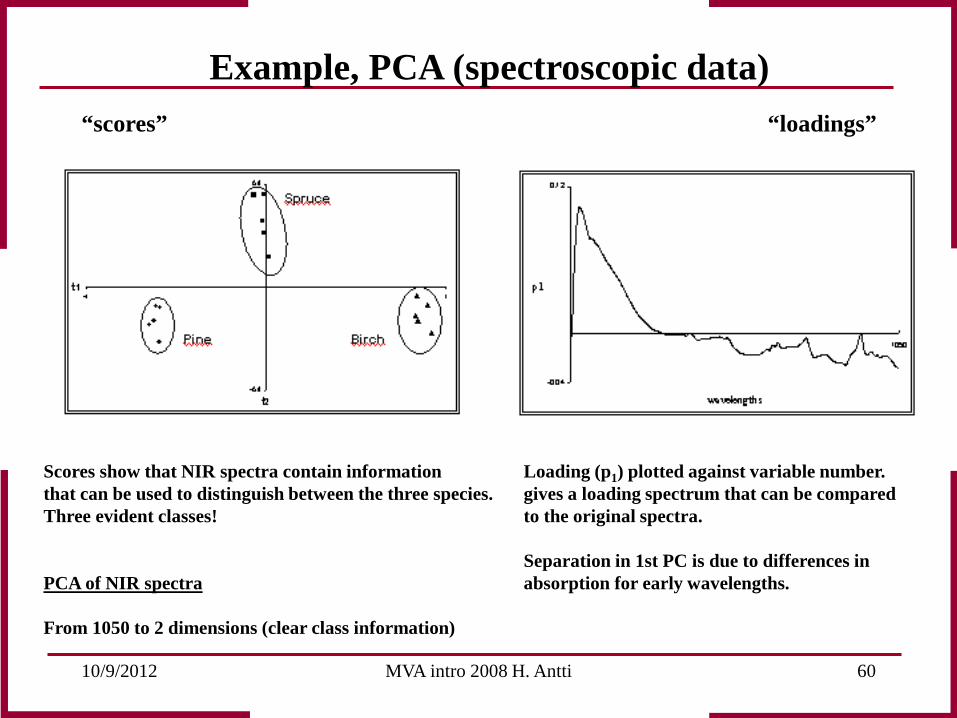
“scores” “loadings”
Scores show that NIR spectra contain information that can be used to distinguish between the three species. Three evident classes! PCA of NIR spectra From 1050 to 2 dimensions (clear class information)
Loading (p1) plotted against variable number. gives a loading spectrum that can be compared to the original spectra. Separation in 1st PC is due to differences in absorption for early wavelengths.
Example, PCA (spectroscopic data)
10/9/2012 MVA intro 2008 H. Antti 61
Conclusion
• Multivariate data - How are they generated - Properties - Definition of problems (Overview, Classification, Regression) • Methods -Univariate -Multivariate (PCA, PCR, PLS, PLS-DA) • Latent variables • Projections • PCA - Basic theory - Model (scores, loadings, residuals) - Interpretation (scores, loadings) - Examples