univariate and multivariate statistical distributions · brief primer on matrix algebra ... reading...

Univariate and Multivariate Statistical Distributions

PRE 906: Structural Equation ModelingLecture #2 – January 28, 2015

PRE 906, SEM: Lecture 2-Distributions

Today’s Class

• Random variables: definitions and types

• Univariate distributions General terminology

Univariate normal/Gaussian

• Brief introduction to matrix algebra

• Multivariate distributions The multivariate normal distribution

PRE 906, SEM: Lecture 2-Distributions 2

Key Questions for Today’s Lecture

1. Why is knowledge about random variables important to learn for use with SEM?

2. What are the two parameters of the univariate normal distribution and what do they govern?

3. What is are matrices and what basic algebraic operations can be conducted such things?

4. What are the two matrices of parameters of the multivariate normal distribution and what do they govern?


RANDOM VARIABLES AND STATISTICAL DISTRIBUTIONS


Why is there a Lecture about Random Variables in SEM Class?

• Random variables are key to statistical analyses: They provide the distributional specifics that accompany assumptions about data

when analyses are conducted They provide the necessary functions to estimate models for specific analyses They also provide a mechanism to describe a set of multivariate data through use

of statistical parameters that we use for scientific inference

• Structural equation models make a number of assumptions that involve random variables Assumptions about the distribution of the data Assumptions about the distribution of error (if any exists) Assumptions about the distribution of the latent variables

• Typically, SEMs have used normal distributions for everything Can be any distribution, though

• This class will introduce you to larger classes of models with normal and non-normal assumptions Therefore your analyses don’t have to be typical better fit to your data


Random Variables

Random: situations in which the certainty of the outcome is unknown and is at least in part due to chance

+

Variable: a value that may change given the scope of a given problem or set of operations

=

Random Variable: a variable whose outcome depends on chance

(possible values might represent the possible outcomes of a yet-to-be-performed experiment)

Today we will denote a random variable with a lower-cased: 𝑥


Key Features of Random Variables

• Random variables each are described by a probability density/mass function (PDF) 𝑓(𝑥) that indicates relative frequency of occurrence A PDF is a mathematical function that gives a rough picture of the distribution

from which a random variable is drawn


Types of Random Variables

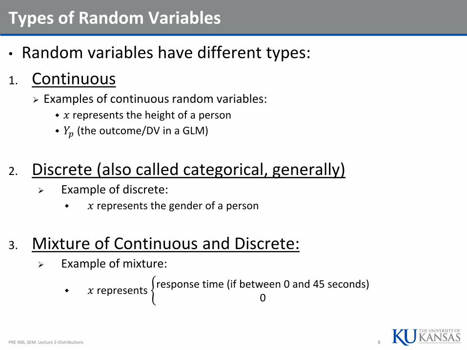
• Random variables have different types:

1. Continuous Examples of continuous random variables:

𝑥 represents the height of a person

𝑌𝑝 (the outcome/DV in a GLM)

2. Discrete (also called categorical, generally) Example of discrete:

𝑥 represents the gender of a person

3. Mixture of Continuous and Discrete: Example of mixture:

𝑥 represents response time (if between 0 and 45 seconds)

0


Uses of Distributions in Data Analysis

• Statistical models make distributional assumptions on various parameters and/or parts of data

• These assumptions govern: How models are estimated

How inferences are made

How missing data are incorporated or modeled within an analysis

• If data do not follow an assumed distribution, inferences may be inaccurate It is important to pick distributions that are plausible for the analysis of the

data you have


CONTINUOUS UNIVARIATE DISTRIBUTIONS


Continuous Univariate Distributions

• To demonstrate how continuous distributions work and look, we will discuss three: Uniform distribution

Normal distribution

Chi-square distribution

• Each are described a set of parameters, which we will later see are what give us our inferences when we analyze data

• What we then do is put constraints on those parameters based on hypothesized effects in data


Uniform Distribution

• The uniform distribution is shown to help set up how continuous distributions work

• For a continuous random variable 𝑥 that ranges from 𝑎, 𝑏 , the uniform probability density function is:

𝑓 𝑥 =1

𝑏 − 𝑎

• The uniform distribution has two parameters: 𝑎 – the lower limit 𝑏 – the upper limit

• 𝑥 ∼ 𝑈 𝑎, 𝑏PRE 906, SEM: Lecture 2-Distributions 12

More on the Uniform Distribution

• To demonstrate how PDFs work, we will try a few values:

• The uniform PDF has the feature that all values of 𝑥 are equally likely across the sample space of the distribution Therefore, you do not see 𝑥 in the PDF 𝑓 𝑥

• The mean of the uniform distribution is 1

2(𝑎 + 𝑏)

• The variance of the uniform distribution is 1

12𝑏 − 𝑎 2

𝒙 𝒂 𝒃 𝒇(𝒙)

.5 0 1 1

1 − 0= 1

.75 0 1 1

1 − 0= 1

15 0 20 1

20 − 0= .05

15 10 20 1

20 − 10= .1


Univariate Normal Distribution

• For a continuous random variable 𝑥 (ranging from −∞ to ∞) the univariate normal distribution function is:

𝑓 𝑥 =1

2𝜋𝜎𝑥2exp −

𝑥 − 𝜇𝑥2

2𝜎𝑥2

• The shape of the distribution is governed by two parameters: The mean 𝜇𝑥 The variance 𝜎𝑥

2

These parameters are called sufficient statistics (they contain all the information about the distribution)

• The skewness (lean) and kurtosis (peakedness) are fixed

• Standard notation for normal distributions is 𝑥 ∼ 𝑁(𝜇𝑥, 𝜎𝑥2)

Read as: “𝑥 follows a normal distribution with a mean 𝜇𝑥 and a variance 𝜎𝑥2”

• Linear combinations of random variables following normal distributions result in a random variable that is normally distributed


Univariate Normal Distribution

𝑓(𝑥)

𝑓 𝑥 gives the height of the curve (relative frequency) for any value of 𝑥, 𝜇𝑥, and 𝜎𝑥2

• R provides this for you directly using the dnorm() function


More of the Univariate Normal Distribution

• To demonstrate how the normal distribution works, we will try a few values:

• The values from 𝑓 𝑥 were obtained by using R The “=rnorm()” function Most statistics packages have a normal distribution function

• The mean of the normal distribution is 𝜇𝑥• The variance of the normal distribution is 𝜎𝑥

2

𝒙 𝝁𝒙 𝝈𝒙𝟐 𝒇(𝒙)

.5 0 1 0.352

.75 0 1 0.301

.5 0 5 0.079

.75 -2 1 0.009

-2 -2 1 0.399


Chi-Square Distribution

• Another frequently used univariate distribution is the Chi-Square distribution Sampling distribution of the variance follows a chi-square distribution

Likelihood ratios follow a chi-square distribution

• For a continuous random variable 𝑥 (ranging from 0 to ∞), the chi-square distribution is given by:

𝑓 𝑥 =1

2𝜈2Γ

𝜈2

𝑥𝜈2−1 exp −

𝑥

2

• Γ ∙ is called the gamma function

• The chi-square distribution is governed by one parameter: 𝜈(the degrees of freedom) The mean is equal to 𝜈; the variance is equal to 2𝜈


(Univariate) Chi-Square Distribution

𝑥

𝑓(𝑥)


FROM MARGINAL DISTRIBUTIONS TO JOINT DISTRIBUTIONS


Moving from One to Multiple Random Variables

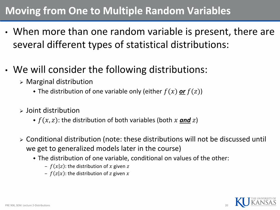
• When more than one random variable is present, there are several different types of statistical distributions:

• We will consider the following distributions: Marginal distribution

The distribution of one variable only (either 𝑓(𝑥) or 𝑓(𝑧))

Joint distribution 𝑓(𝑥, 𝑧): the distribution of both variables (both 𝑥 and 𝑧)

Conditional distribution (note: these distributions will not be discussed until we get to generalized models later in the course) The distribution of one variable, conditional on values of the other:

– 𝑓 𝑥 𝑧 : the distribution of 𝑥 given 𝑧

– 𝑓 𝑧 𝑥 : the distribution of 𝑧 given 𝑥


Marginal Distributions

• Marginal distributions are what we have worked with exclusively up to this point: they represent the distribution of one variable by itself

Continuous univariate distributions: Uniform

Normal

Chi-square

Categorical distributions (also not discussed until later in the course): Bernoulli

Binomial

Multinomial

Poisson


Joint Distributions

• Joint distributions describe the distribution of more than one variable, simultaneously Representations of multiple variables collected

• Commonly, the joint distribution function is denoted with all random variables separated by commas In our example, 𝑓 𝑥, 𝑧 is the joint distribution of the outcome of a random

variable 𝑥 and a random variable 𝑧

• Joint distributions are multivariate distributions We will cover the continuous multivariate normal distribution today

• Most joint distributions are described symbolically using matrix algebra (so we will discuss that briefly)


BRIEF PRIMER ON MATRIX ALGEBRA

For Reading and Deciphering Multivariate Distributions


Definitions

• We begin this section with some general definitions (from dictionary.com): Matrix:

1. A rectangular array of numeric or algebraic quantities subject to mathematical operations

2. The substrate on or within which a fungus grows

Algebra:

1. A branch of mathematics in which symbols, usually letters of the alphabet, represent numbers or members of a specified set and are used to represent quantities and to express general relationships that hold for all members of the set

2. A set together with a pair of binary operations defined on the set. Usually, the set and the operations include an identity element, and the operations are commutative or associative


Why Learn Matrix Algebra

• Matrix algebra can seem very abstract from the purposes of this class (and statistics in general)

• Learning matrix algebra is important for: Understanding how statistical methods work

And when to use them (or not use them)

Understanding what statistical methods mean

Reading and writing results from new statistical methods

• Today’s class is the first lecture of learning the language of multivariate statistics and structural equation modeling


DATA EXAMPLE AND R


A Guiding Example

• To demonstrate matrix algebra, we will make use of data

• Imagine that I collected data SAT test scores for both the Math (SATM) and Verbal (SATV) sections of 1,000 students

• The descriptive statistics of this data set are given below:


DEFINITIONS OF MATRICES, VECTORS, AND SCALARS


Matrices

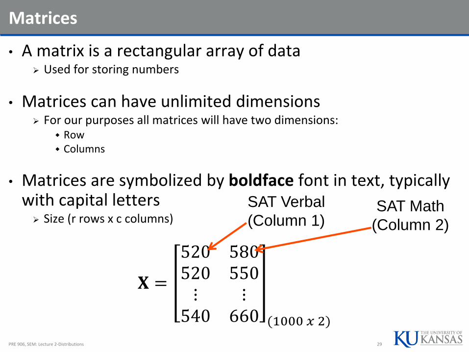
• A matrix is a rectangular array of data Used for storing numbers

• Matrices can have unlimited dimensions For our purposes all matrices will have two dimensions:

Row Columns

• Matrices are symbolized by boldface font in text, typically with capital letters Size (r rows x c columns)

𝐗 =

520 580520 550⋮ ⋮

540 660 (1000 𝑥 2)


SAT Verbal

(Column 1)SAT Math

(Column 2)

Vectors

• A vector is a matrix where one dimension is equal to size 1 Column vector: a matrix of size 𝑟 𝑥 1

𝒙∙1 =

520520⋮

540 1000 𝑥 1

Row vector: a matrix of size 1 𝑥 𝑐𝒙1∙ = 520 580 1 𝑥 2

• Vectors are typically written in boldface font text, usually with lowercase letters

• The dots in the subscripts 𝒙∙1 and 𝒙1∙ represent the dimension aggregated across in the vector

𝒙1∙ is the first row and all columns of 𝐗

𝒙∙1 is the first column and all rows of 𝐗

Sometimes the rows and columns are separated by a comma (making it possible to read double-digits in either dimension)


Matrix Elements

• A matrix (or vector) is composed of a set of elements Each element is denoted by its position in the matrix (row and column)

• For our matrix of data 𝐗 (size 1000 rows and 2 columns), each element is denoted by:

𝑥𝑖𝑗

The first subscript is the index for the rows: i = 1,…,r (= 1000)

The second subscript is the index for the columns: j = 1,…,c (= 2)

𝐗 =

𝑥11 𝑥12𝑥21 𝑥22⋮ ⋮

𝑥1000,1 𝑥1000,2 (1000 𝑥 2)


Scalars

• A scalar is just a single number

• The name scalar is important: the number “scales” a vector – it can make a vector “longer” or “shorter”

• Scalars are typically written without boldface:𝑥11 = 520

• Each element of a matrix is a scalar


Matrix Transpose

• The transpose of a matrix is a reorganization of the matrix by switching the indices for the rows and columns

𝐗 =

520 580520 550⋮ ⋮

540 660 (1000 𝑥 2)

𝐗𝑇 =520 520 ⋯ 540580 550 ⋯ 660 2 𝑥 1000

• An element 𝑥𝑖𝑗 in the original matrix 𝐗 is now 𝑥𝑗𝑖 in the transposed matrix 𝐗𝑇

• Transposes are used to align matrices for operations where the sizes of matrices matter (such as matrix multiplication)


Types of Matrices

• Square Matrix: A square matrix has the same number of rows and columns Correlation/covariance matrices are square matrices

• Diagonal Matrix: A diagonal matrix is a square matrix with non-zero diagonal elements (𝑥𝑖𝑗 ≠ 0 for 𝑖 = 𝑗) and zeros

on the off-diagonal elements (𝑥𝑖𝑗 = 0 for 𝑖 ≠ 𝑗):

𝐀 =2.759 0 00 1.643 00 0 0.879

• Symmetric Matrix: A symmetric matrix is a square matrix with all elements reflected across the diagonal (𝑎𝑖𝑗 = 𝑎𝑗𝑖) Correlation and covariance matrices are symmetric matrices


VECTORS


Vectors in Space…

• Vectors (row or column) can be represented as lines on a Cartesian coordinate system (a graph)

• Consider the vectors: 𝐚 =12

and 𝐛 =23

• A graph of these vectors would be:

• Question: how would a column vector for each of our example variables (SATM and SATV) be plotted?


Vector Addition

• Vectors can be added together resulting in a new vector

• Vector addition is done element-wise, by adding each of the respective elements together: The new vector has the same number of rows and columns

𝐜 = 𝐚 + 𝐛 =12

+23

=35

Geometrically, this creates a new vector along either of the previous two Starting at the origin and ending at a new point in space

• In Data: a new variable (say, SAT total) is the result of vector addition

𝑺𝑨𝑻𝑻𝑶𝑻𝑨𝑳 = 𝒙.1 + 𝒙.2


Vector Addition: Geometrically


Vector Multiplication by Scalar

• Vectors can be multiplied by scalars All elements are multiplied by the scalar

𝐝 = 2𝐚 = 212

=24

• Scalar multiplication changes the length of the vector:

𝐝 = 22 + 42 = 20 = 4.47

• This is where the term scalar comes from: a scalar ends up “rescaling” (resizing) a vector

• In Data: the GLM (where X is a matrix of data) the fixed effects (slopes) are scalars multiplying the data


Scalar Multiplication: Geometrically


Linear Combinations

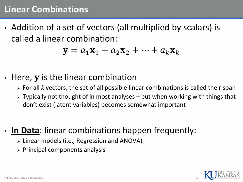
• Addition of a set of vectors (all multiplied by scalars) is called a linear combination:

𝐲 = 𝑎1𝐱1 + 𝑎2𝐱2 +⋯+ 𝑎𝑘𝐱𝑘

• Here, 𝐲 is the linear combination For all k vectors, the set of all possible linear combinations is called their span

Typically not thought of in most analyses – but when working with things that don’t exist (latent variables) becomes somewhat important

• In Data: linear combinations happen frequently: Linear models (i.e., Regression and ANOVA)

Principal components analysis


Linear Dependencies

• A set of vectors are said to be linearly dependent if𝑎1𝐱1 + 𝑎2𝐱2 +⋯+ 𝑎𝑘𝐱𝑘 = 0

-and-

𝑎1, 𝑎2, … , 𝑎𝑘 are all not zero

• Example: let’s make a new variable – SAT Total:𝐒𝐀𝐓𝐭𝐨𝐭𝐚𝐥 = 1 ∗ 𝐒𝐀𝐓𝐕 + 1 ∗ 𝐒𝐀𝐓𝐌

• The new variable is linearly dependent with the others:1 ∗ 𝐒𝐀𝐓𝐕 + 1 ∗ 𝐒𝐀𝐓𝐌+ (−1) ∗ 𝐒𝐀𝐓𝐭𝐨𝐭𝐚𝐥 = 𝟎

• In Data: (multi) collinearity is a linear dependency. Linear dependencies are bad for analyses that use matrix inverses


Inner (Dot) Product of Vectors

• An important concept in vector geometry is that of the inner product of two vectors The inner product is also called the dot product

𝐚 ∙ 𝐛 = 𝐚𝑇𝐛 = 𝑎11𝑏11 + 𝑎21𝑏21 +⋯+ 𝑎𝑁1𝑏𝑁1 =

𝑖=1

𝑁

𝑎𝑖1𝑏𝑖1

• The dot or inner product is related to the angle between vectors and to the projection of one vector onto another

• From our example: 𝐚 ∙ 𝐛 = 1 ∗ 2 + 2 ∗ 3 = 8

• From our data: 𝒙.1 ⋅ 𝒙.2 = 251,928,400• In data: the angle between vectors is related to the correlation

between variables and the projection is related to regression/ANOVA/linear models


MATRIX ALGEBRA


Moving from Vectors to Matrices

• A matrix can be thought of as a collection of vectors Matrix operations are vector operations on steroids

• Matrix algebra defines a set of operations and entities on matrices

I will present a version meant to mirror your previous algebra experiences

• Definitions: Identity matrix Zero vector Ones vector

• Basic Operations: Addition Subtraction Multiplication “Division”


Matrix Addition and Subtraction

• Matrix addition and subtraction are much like vector addition/subtraction

• Rules: Matrices must be the same size (rows and columns)

• Method: The new matrix is constructed of element-by-element addition/subtraction of

the previous matrices

• Order: The order of the matrices (pre- and post-) does not matter


Matrix Addition/Subtraction


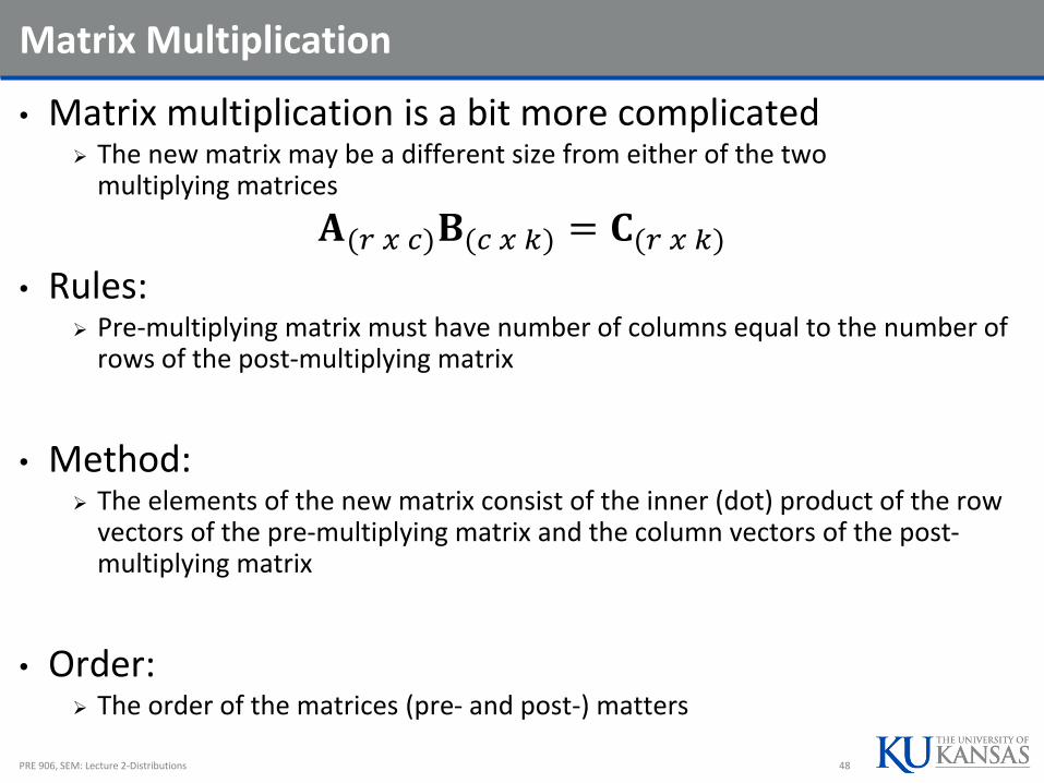
Matrix Multiplication

• Matrix multiplication is a bit more complicated The new matrix may be a different size from either of the two

multiplying matrices

𝐀(𝑟 𝑥 𝑐)𝐁(𝑐 𝑥 𝑘) = 𝐂(𝑟 𝑥 𝑘)

• Rules: Pre-multiplying matrix must have number of columns equal to the number of

rows of the post-multiplying matrix

• Method: The elements of the new matrix consist of the inner (dot) product of the row

vectors of the pre-multiplying matrix and the column vectors of the post-multiplying matrix

• Order: The order of the matrices (pre- and post-) matters


Matrix Multiplication


Multiplication in Statistics

• Many statistical formulae with summation can be re-expressed with matrices

• A common matrix multiplication form is: 𝐗𝑇𝐗 Diagonal elements: 𝑖=1

𝑁 𝑋𝑖2

Off-diagonal elements: 𝑖=1𝑁 𝑋𝑖𝑎𝑋𝑖𝑏

• For our SAT example:

𝐗𝑇𝐗 =

𝑖=1

𝑁

𝑆𝐴𝑇𝑉𝑖2

𝑖=1

𝑁

𝑆𝐴𝑇𝑉𝑖𝑆𝐴𝑇𝑀𝑖

𝑖=1

𝑁

𝑆𝐴𝑇𝑉𝑖𝑆𝐴𝑇𝑀𝑖

𝑖=1

𝑁

𝑆𝐴𝑇𝑀𝑖2

=251,797,800 251,928,400251,928,400 254,862,700


Identity Matrix

• The identity matrix is a matrix that, when pre- or post-multiplied by another matrix results in the original matrix:

𝐀𝐈 = 𝐀𝐈𝐀 = 𝐀

• The identity matrix is a square matrix that has: Diagonal elements = 1

Off-diagonal elements = 0

𝐼 3 𝑥 3 =1 0 00 1 00 0 1


Zero Vector

• The zero vector is a column vector of zeros

𝟎(3 𝑥 1) =000

• When pre- or post- multiplied the result is the zero vector:𝐀𝟎 = 𝟎𝟎𝐀 = 𝟎


Ones Vector

• A ones vector is a column vector of 1s:

𝟏(3 𝑥 1) =111

• The ones vector is useful for calculating statistical terms, such as the mean vector and the covariance matrix


Matrix “Division”: The Inverse Matrix

• Division from algebra: First:

𝑎

𝑏=

1

𝑏𝑎 = 𝑏−1𝑎

Second: 𝑎

𝑎= 1

• “Division” in matrices serves a similar role For square and symmetric matrices, an inverse matrix is a matrix that when

pre- or post- multiplied with another matrix produces the identity matrix:𝐀−1𝐀 = 𝐈𝐀𝐀−𝟏 = 𝐈

• Calculation of the matrix inverse is complicated Even computers have a tough time

• Not all matrices can be inverted Non-invertible matrices are called singular matrices

In statistics, singular matrices are commonly caused by linear dependencies


The Inverse

• In data: the inverse shows up constantly in statistics Models which assume some type of (multivariate) normality need an inverse

covariance matrix

• Using our SAT example Our data matrix was size (1000 x 2), which is not invertible

However 𝐗𝑇𝐗 was size (2 x 2) – square, and symmetric

𝐗𝑇𝐗 =251,797,800 251,928,400251,928,400 254,862,700

The inverse is:

𝐗𝑇𝐗 −1 =3.61𝐸 − 7 −3.57𝐸 − 7−3.57𝐸 − 7 3.56𝐸 − 7


Matrix Algebra Operations

• 𝐀 + 𝐁 + 𝐂 =𝐀 + (𝐁 + 𝐂)

• 𝐀 + 𝐁 = 𝐁 + 𝐀

• 𝑐 𝐀 + 𝐁 = 𝑐𝐀 + 𝑐𝐁

• 𝑐 + 𝑑 𝐀 = 𝑐𝐀 + 𝑑𝐀

• 𝐀 + 𝐁 𝑇 = 𝐀𝑇 + 𝐁𝑇

• 𝑐𝑑 𝐀 = 𝑐(𝑑𝐀)

• 𝑐𝐀 𝑇 = 𝑐𝐀𝑇

• 𝑐 𝐀𝐁 = 𝑐𝐀 𝐁

• 𝐀 𝐁𝐂 = 𝐀𝐁 𝐂

• 𝐀 𝐁 + 𝐂 = 𝐀𝐁 + 𝐀𝐂

• 𝐀𝐁 𝑇 = 𝐁𝑇𝐀𝑇

• For 𝑥𝑗 such that 𝐴𝑥𝑗 exists:

𝑗=1

𝑁

𝐀𝐱𝑗 =𝐀

𝑗=1

𝑁

𝐱𝑗

𝑗=1

𝑁

𝐀𝐱𝑗 𝐀𝐱𝑗𝑇=

𝐀

𝑗=1

𝑁

𝐱𝑗𝐱𝑗𝑇 𝐀𝑇


BIVARIATE NORMAL DISTRIBUTION

A Multivariate Distribution with Two Variables


Bivariate Normal Distribution

• The bivariate normal is a joint distribution for two variables Both variable is normally distributed marginally (by itself)

Together, they form a bivariate normal distribution

• The bivariate normal density provides the relatively frequency of observing any pair of observations, 𝐱𝑖 = 𝑥𝑖1 𝑥𝑖2

𝑓 𝑥1, 𝑥2 =1

2𝜋𝜎𝑥1𝜎𝑥2 1 − 𝜌2exp −

𝑧

2 1 − 𝜌2

Where

𝑧 =𝑥𝑖1 − 𝜇𝑥1

2

𝜎𝑥12 −

2𝜌 𝑥𝑖1 − 𝜇𝑥1 𝑥𝑖2 − 𝜇𝑥2𝜎1𝜎2

+𝑥𝑖2 − 𝜇𝑥2

2

𝜎𝑥22


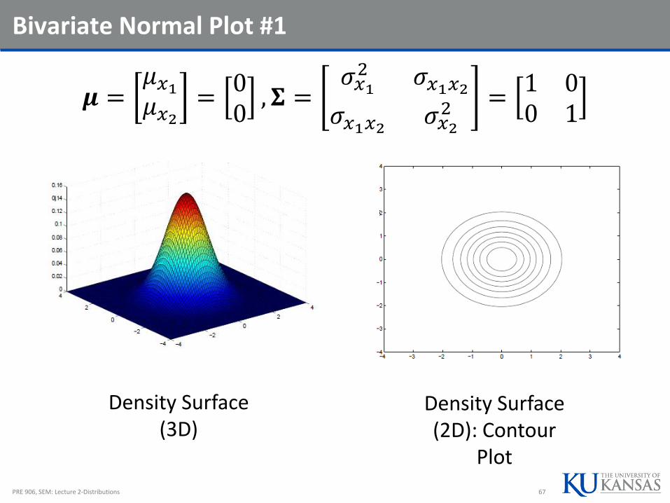
Bivariate Normal Plot #1

𝝁 =𝜇𝑥1𝜇𝑥2

=00

, 𝚺 =𝜎𝑥12 𝜎𝑥1𝑥2

𝜎𝑥1𝑥2 𝜎𝑥22 =

1 00 1

Density Surface (3D)

Density Surface (2D): Contour

Plot




=00



1 .5.5 1



Plot


MULTIVARIATE NORMAL DISTRIBUTIONS (VARIABLES ≥ 2)


Multivariate Normal Distribution

• The multivariate normal distribution is the generalization of the univariate normal distribution to multiple variables The bivariate normal distribution just shown is part of the MVN

• The MVN provides the relative likelihood of observing all V variables for a subject p simultaneously:

𝐱𝑝 = 𝑥𝑝1 𝑥𝑝2 … 𝑥𝑝𝑉

• The multivariate normal density function is:

𝑓 𝐱𝑝 =1

2𝜋𝑉2 𝚺

12

exp −𝐱𝑝𝑇 − 𝝁

𝑇𝚺−1 𝐱𝑝

𝑇 − 𝝁

2


The Multivariate Normal Distribution

𝑓 𝐱𝑝 =1

2𝜋𝑉2 𝚺

12



𝑇 − 𝝁

2

• The mean vector is 𝝁 =

𝜇𝑥1𝜇𝑥2⋮

𝜇𝑥𝑉

• The covariance matrix is 𝚺 =

𝜎𝑥12 𝜎𝑥1𝑥2 ⋯ 𝜎𝑥1𝑥𝑉

𝜎𝑥1𝑥2 𝜎𝑥22 ⋯ 𝜎𝑥2𝑥𝑉

⋮ ⋮ ⋱ ⋮𝜎𝑥1𝑥𝑉 𝜎𝑥2𝑥𝑉 ⋯ 𝜎𝑥𝑉

2

The covariance matrix must be non-singular (invertible)PRE 906, SEM: Lecture 2-Distributions 63

Comparing Univariate and Multivariate Normal Distributions

• The univariate normal distribution:

𝑓 𝑥𝑝 =1

2𝜋𝜎2exp −

𝑥 − 𝜇 2

2𝜎2

• The univariate normal, rewritten with a little algebra:

𝑓 𝑥𝑝 =1

2𝜋12|𝜎2|

12

exp −𝑥 − 𝜇 𝜎−

12 𝑥 − 𝜇

2

• The multivariate normal distribution

𝑓 𝐱𝑝 =1

2𝜋𝑉2 𝚺

12



𝑇 − 𝝁

2

When 𝑉 = 1 (one variable), the MVN is a univariate normal distribution


The Exponent Term

• The term in the exponent (without the −1

2) is called the

squared Mahalanobis Distance

𝑑2 𝒙𝑝 = 𝐱𝑝𝑇 − 𝝁


𝑇 − 𝝁

Sometimes called the statistical distance

Describes how far an observation is from its mean vector, in standardized units

Like a multivariate Z score (but, if data are MVN, is actually distributed as a 𝜒2variable with DF = number of variables in X)

Can be used to assess if data follow MVN


Multivariate Normal Notation

• Standard notation for the multivariate normal distribution of v variables is 𝑁𝑣 𝝁, 𝚺 Our SAT example would use a bivariate normal: 𝑁2 𝝁, 𝚺

• In data: The multivariate normal distribution serves as the basis for most every

statistical technique commonly used in the social and educational sciences General linear models (ANOVA, regression, MANOVA)

General linear mixed models (HLM/multilevel models)

Factor and structural equation models (EFA, CFA, SEM, path models)

Multiple imputation for missing data

Simply put, the world of commonly used statistics revolves around the multivariate normal distribution Understanding it is the key to understanding many statistical methods




=00



1 00 1




Plot

Bivariate Normal Plot #2 (Multivariate Normal)


=00



1 .5.5 1




Plot

Multivariate Normal Properties

• The multivariate normal distribution has some useful properties that show up in statistical methods

• If 𝐗 is distributed multivariate normally:

1. Linear combinations of 𝐗 are normally distributed

2. All subsets of 𝐗 are multivariate normally distributed

3. A zero covariance between a pair of variables of 𝐗implies that the variables are independent

4. Conditional distributions of 𝐗 are multivariate normal


WRAPPING UP AND REFOCUSING


Key Questions for Today’s Lecture

1. Why is knowledge about random variables important to learn for use with SEM?

2. What are the two parameters of the univariate normal distribution and what do they govern?

3. What is are matrices and what basic algebraic operations can be conducted such things?

4. What are the two matrices of parameters of the multivariate normal distribution and what do they govern?


Concluding Remarks

• The univariate and multivariate normal distributions serve as the backbone of the most frequently used statistical procedures They are very robust and very useful

• Understanding their form and function will help you learn about a whole host of statistical routines immediately This course is essentially a course based in normal distributions

• Inspecting normality is a tricky thing More often than not, data will not be normal More often than not, no one will check (don’t ask, don’t tell)

• Next week: linear models in matrices, repeated measures ANOVA, Multivariate ANOVA Classical statistics – described as a background for modern methods


univariate and multivariate statistical distributions · brief primer on matrix algebra ... reading...

Documents