“High‐redshi+ dust emission and CO emission predic7ons for ALMA” 

Mul$wavelength Views of the ISM in High‐Redshi9 Galaxies, San7ago, 27/06/2011 

Juan E. Gonzalez, ESO, Garching 

TAMASIS project 

‐  People: ‐  ESO (Eelco van Kampen) ‐  CE Saclay (Marc Sauvage, Pierre Chanial, Barbey Nicolas) ‐  IAS Orsay (Abergel Alain) ‐  Leiden (Paul van der Werf, Meijerink Rowin) 

‐  Generate tools to produce mock sub‐mm maps predic7ons for Herschel, SCUBA‐2 & ALMA. 

Models 

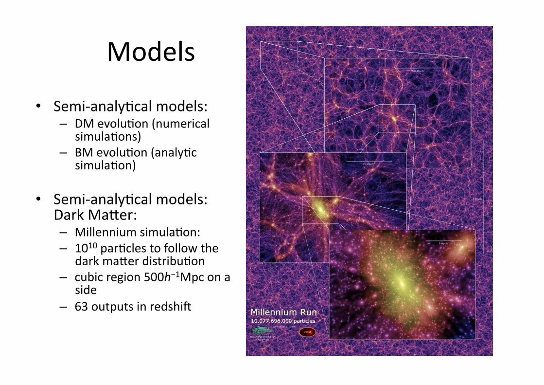
•  Semi‐analy7cal models: –  DM evolu7on (numerical 

simula7ons) –  BM evolu7on (analy7c 

simula7on) 

•  Semi‐analy7cal models: Dark Ma_er: –  Millennium simula7on: –  1010 par7cles to follow the 

dark ma_er distribu7on –  cubic region 500h−1Mpc on a 

side –  63 outputs in redshi+ 

Models 

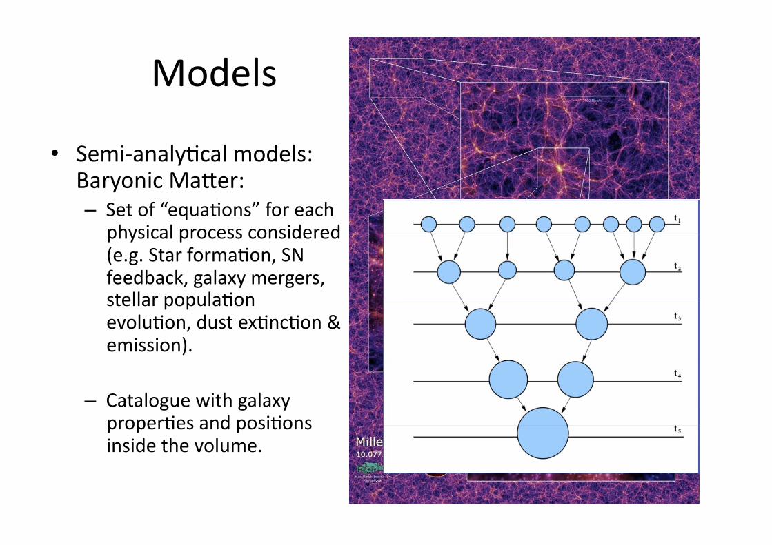
•  Semi‐analy7cal models: Baryonic Ma_er: –  Set of “equa7ons” for each  

physical process considered (e.g. Star forma7on, SN feedback, galaxy mergers, stellar popula7on evolu7on, dust ex7nc7on & emission). 

–  Catalogue with galaxy proper7es and posi7ons inside the volume. 

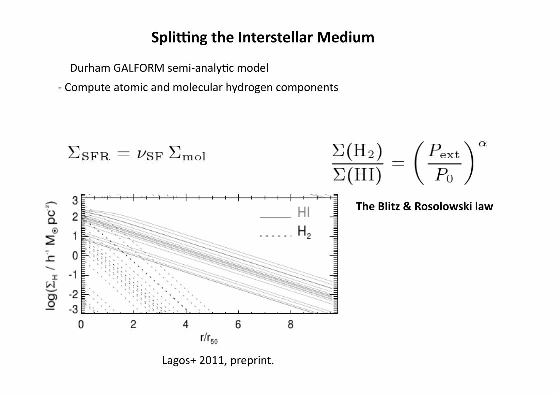
The Blitz & Rosolowski law 

SpliCng the Interstellar Medium 

‐ Compute atomic and molecular hydrogen components 

Lagos+ 2011, preprint. 

Durham GALFORM semi‐analy7c model 

Lightcone proper7es 

•  The orienta7on of the lightcone is given by the vector: (3, 4, 1).  

•  With no repe77on of  galaxies in the Simula7on: – Gives a area of about 2 square deg. – Out to z~4.2 

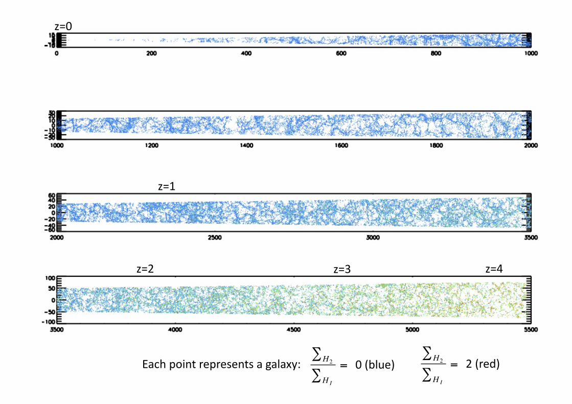
z=1 

z=2  z=3  z=4 

Each point represents a galaxy: 

€

∑H2

∑H I

= 0 (blue) 

€

∑H2

∑H I

= 2 (red) 

z=0 

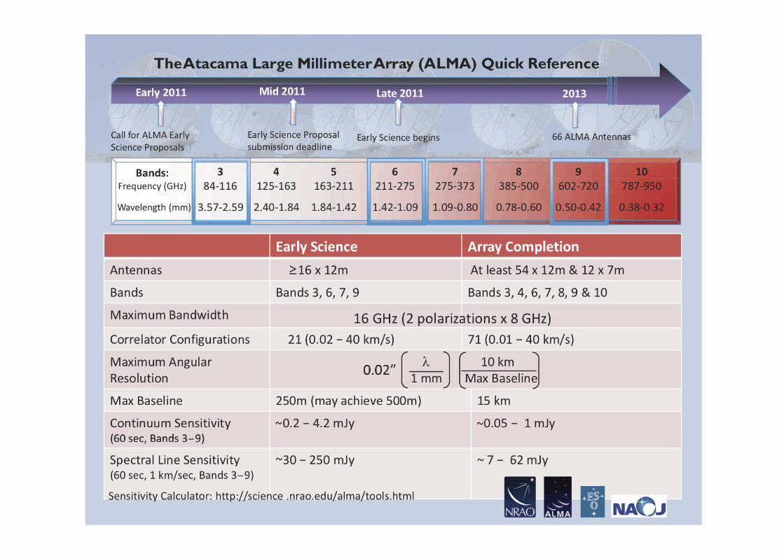
For band 3 we can iden7fy transi7ons:  CO (2‐>1) [230.5Ghz] [1301μm]                in redshi+ range: z= 1 ‐> 1.7  CO (3‐>2) [345.8Ghz] [867.5μm]               in redshi+ range: z= 2 ‐> 3.1  CO (4‐>3) [461.0Ghz] [650.8μm]               in redshi+ range: z= 3 ‐> 4.5 

In ALMA: 

CO Lines es7ma7ons Evolution of the HI and H2 gas content 9

ICO/Kkms!1 =NH2

/cm!2

X! 10!20. (4)

Here NH2is the column density of H2 and ICO is the integrated

CO(1 " 0) line intensity per unit surface area. The value of Xhas been inferred observationally in a few galaxies, mainly throughvirial estimations. Typical estimates for normal spiral galaxiesrange between X # 2.0 " 3.5 (e.g. Young & Scoville 1991;Boselli et al. 2002; Blitz et al. 2007). However, systematic varia-tions in the value ofX are both, theoretically predicted and inferredobservationally. For instance, theoretical calculations predict thatlow metallicities, characteristic of dwarf galaxies, or high densitiesand large optical depths of molecular clumps in starburst galaxies,should change X by a factor of up to 5 " 10 in either direction(e.g. Bell et al. 2007; Meijerink et al. 2007; Bayet et al. 2009). Ob-servations of dwarf galaxies favour larger conversion factors (e.g.X # 7; e.g. Boselli et al. 2002), while the opposite holds in star-burst galaxies (e.g. X # 0.5; e.g. Meier & Turner 2004). Thissuggests a metallicity-dependent conversion factor X. However,estimates of the correlation between X and metallicity in nearbygalaxies vary significantly, from finding no correlation, when virialequilibrium of giant molecular clouds (GMCs) is assumed (e.g.Young & Scoville 1991; Blitz et al. 2007), to correlations as strongasX $ (Z/Z")

!1, when the total gas content is inferred from thedust content on assuming metallicity dependent dust-to-gas ratios(e.g. Guelin et al. 1993; Boselli et al. 2002).

We estimate the CO(1" 0) LF by using different conversionfactors favoured by the observational estimates described above.The top panel of Fig. 9 shows the CO(1 " 0) LF at z = 0 whendifferent constant conversion factors are assumed (i.e. independentof galaxy properties; solid lines). Observational estimates of theCO(1"0) LF, made using aB-band and a 60µm selected sample,are plotted using symbols (Keres et al. 2003). The model slightlyunderestimates the number density at L! forX > 1, but gives goodagreement at fainter and at brighter luminosities for sufficientlylarge values of X (such as the ones inferred in normal spiral galax-ies). In the predicted CO(1" 0) LF we include all galaxies with aLCO > 103 Jy km/sMpc2, while the LFs from Keres et al. wereinferred from samples of galaxies selected using 60µm or B-bandfluxes. These criteria might bias the LF towards galaxies with largeamounts of dust or large recent SF. More data is needed from blindCO surveys in order to characterise the CO LF in non-biased sam-ples of galaxies. This will be possible with new instruments suchas the LMT.

In order to illustrate how much our predictions for theCO(1"0) LF at z = 0 vary when adopting a metallicity-dependentconversion factor, X(Z), inferred independently from observa-tions, we also plot in the top panel of Fig. 9 the LF when theX(Z) relation from Boselli et al. (2002) is adopted (dashed line),log(X ) = 0.5+0.2

!0.2 " 1.02+0.05!0.05 log(Z/Z"). Note that this correla-

tion was determined using a sample of 12 galaxies withCO(1"0)luminosities in quite a narrow range, LCO # 5 ! 105 " 5 !

106 Jy km/sMpc2. On adopting this conversion factor, the modellargely underestimates the break of the LF. This is due to the contri-bution of galaxies with different metallicities to theCO(1" 0) LF,as shown in the bottom panel of Fig. 9. The faint-end is dominatedby low-metallicity galaxies (Z < Z"/3), while high-metallicitygalaxies (Z > Z"/3) dominate the bright-end. A smaller Xfor low-metallicity galaxies combined with a larger X for high-metallicity galaxies would give better agreement with the observeddata. However, such a dependence of X on metallicity is oppositeto that inferred by Boselli et al.

By considering a dependence of X on metallicity alone weare ignoring possible variations with other physical propertieswhich could influence the state of GMCs, such as the interstel-lar far-UV radiation field and variations in the column densityof gas (see for instance Pelupessy et al. 2006; Bayet et al. 2009;Pelupessy & Papadopoulos 2009; Papadopoulos 2010). A more de-tailed calculation of the CO LF which takes into account the char-acteristics of the local ISM environment is beyond the scope of thispaper and is addressed in a forthcoming paper (Lagos et al. 2011,in prep.). For the next subsection, we will assume X = 3.5 forquiescent SF and X = 0.5 for starbursts,

For simplicity, in the next subsection we use a fixed CO(1 "

0)-H2 conversion factor of X = 3.5 for galaxies undergoing qui-escent SF and X = 0.5 for those experiencing starbursts. In thecase of galaxies undergoing both SF modes, we use X = 3.5 andX = 0.5 for the quiescent and the burst components, respectively,following the discussion above.

4.2.2 Evolution of the H2 mass function

At high-redshift, measurements of the CO(J % J" 1) LF are notcurrently available. ALMA will, however, provide measurementsof molecular emission lines in high redshift galaxies with high ac-curacy. We therefore present in Fig. 10 predictions for the H2 MFand CO(1" 0) LF up to z = 8.

The high-mass end of the H2 MF shows strong evolution fromz = 8 to z = 4, with the number density of galaxies increasingby an order of magnitude. In contrast, the number density of lowH2 mass galaxies stays approximately constant over the same red-shift range. From z = 4 to z = 2 the H2 MF hardly evolves, withthe number density of galaxies remaining the same over the wholemass range. From z = 2 to z = 0, the number density of massivegalaxies decreases by an order of magnitude, while the low-massend decreases only by a factor # 3. The peak in the number den-sity of massive H2 galaxies at z = 2 " 3 coincides with the peakof the SF activity (see L10; Fanidakis et al. 2010), in which hugeamounts of H2 are consumed forming new stars. The following de-crease in the number density at z < 2 overlaps with strong galacticsize evolution, where galaxies at lower redshift are systematicallylarger than their high redshift counterparts, reducing the gas sur-face density and therefore, the H2 fraction. We return to this pointin §5. The peak in the number density of high H2 mass galaxies atz = 2 " 3 and the following decrease, contrasts with the mono-tonic increase in the number density of high HI mass galaxies withtime, suggesting a strong evolution of the H2/HI global ratio withredshift. We come back to this point in §6.

The evolution of the CO(1" 0) LF with redshift is shown inthe bottom panel of Fig. 10. Note that the z = 0 LF is very similarto the one shown in the bottom panel of Fig. 9, in which we assumea fixed CO-H2 conversion X = 3.5 for all galaxies. This is due tothe low number of starburst events at z = 0. However, at higherredshifts, starbursts contribute more to the LF; the most luminousevents at high redshift, in terms of CO luminosity, correspond tostarbursts (see §4.2.3).

Recently Geach et al. (2011) compared the evolution of theobserved molecular-to-(stellar plus molecular mass) ratio (whichapproximates to the gas-to-baryonic ratio if the HI fraction issmall), fgas = Mmol/(Mstellar +Mmol), with predictions for theBow06.BR model, and found that the model gives a good match tothe observed fgas evolution after applying the same observationalselection cuts.

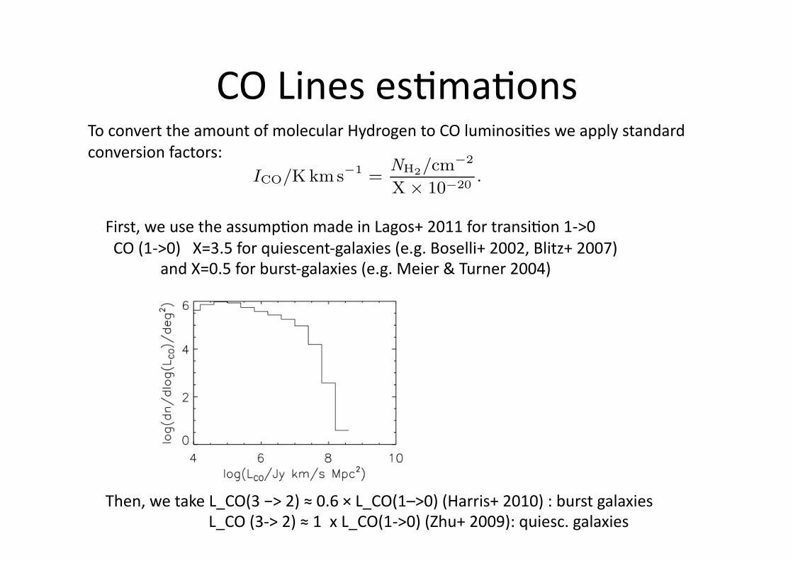
First, we use the assump7on made in Lagos+ 2011 for transi7on 1‐>0   CO (1‐>0)   X=3.5 for quiescent‐galaxies (e.g. Boselli+ 2002, Blitz+ 2007)              

      and X=0.5 for burst‐galaxies (e.g. Meier & Turner 2004) 

Then, we take L_CO(3 −> 2) ≈ 0.6 × L_CO(1–>0) (Harris+ 2010) : burst galaxies                           L_CO (3‐> 2) ≈ 1  x L_CO(1‐>0) (Zhu+ 2009): quiesc. galaxies 

To convert the amount of molecular Hydrogen to CO luminosi7es we apply standard  conversion factors: 

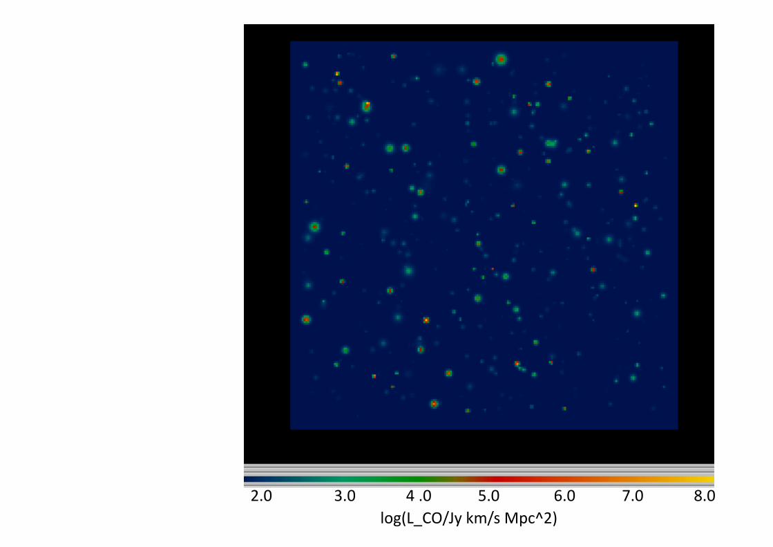
log(L_CO/Jy km/s Mpc^2) 2.0                3.0             4 .0            5.0              6.0            7.0             8.0     

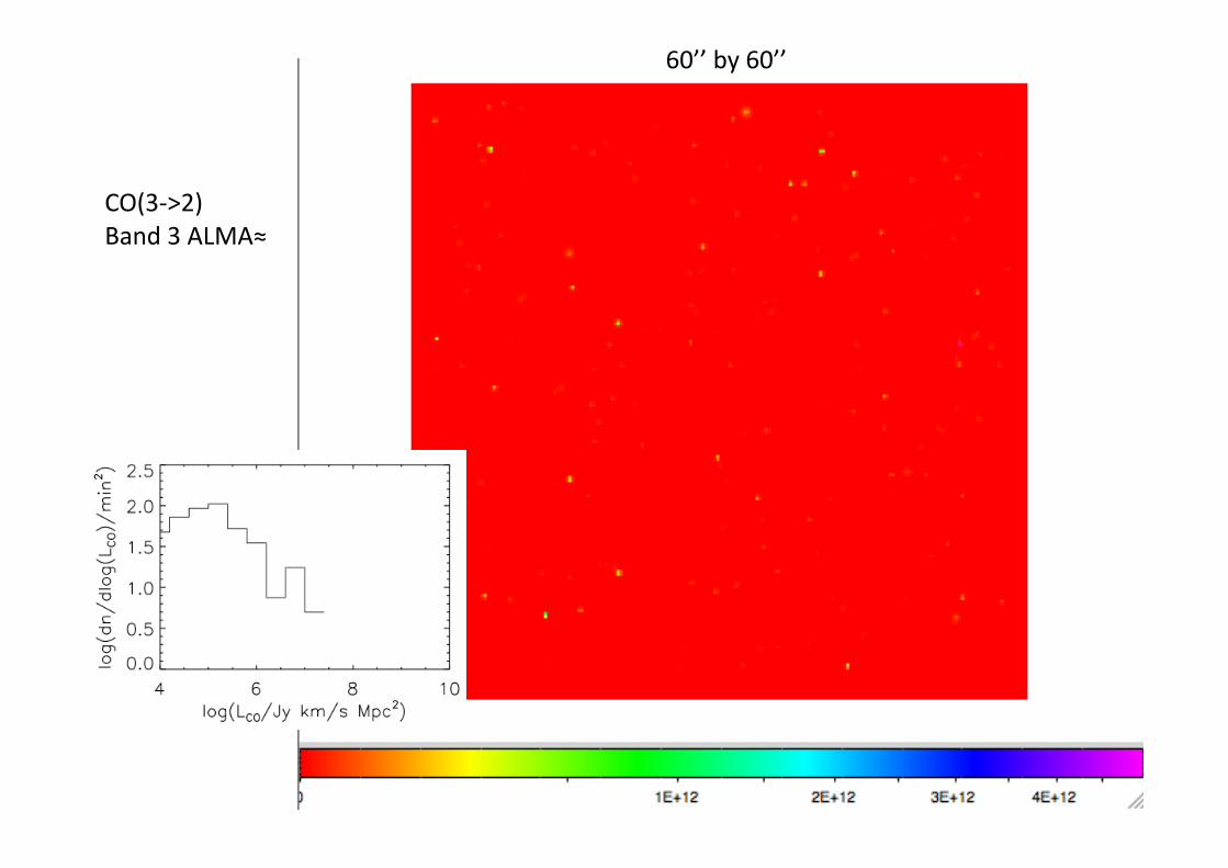
CO(3‐>2)  Band 3 ALMA≈ 

60’’ by 60’’ 

(L_CO/Jy km/s Mpc^2) 

CO(3‐>2)  Band 3 ALMA≈ 

60’’ by 60’’ 

Summary 

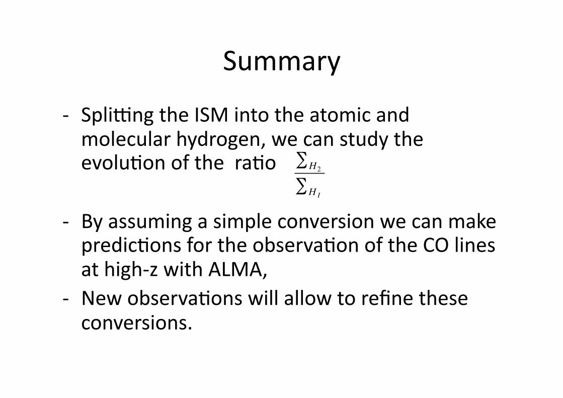
‐  Splixng the ISM into the atomic and molecular hydrogen, we can study the evolu7on of the  ra7o 

‐  By assuming a simple conversion we can make predic7ons for the observa7on of the CO lines at high‐z with ALMA, 

‐  New observa7ons will allow to refine these conversions. 

€

∑H2

∑H I