muscle activity: from d-flow to rage
TRANSCRIPT

Muscle Activity: From D-Flow to RAGE
Small project 2013 (Game and Media Technology)
Name: Jorim Geers
Student number: 3472345
Supervisor: Nicolas Pronost
Date: January 22, 2014

2
Table of contents 1. Introduction ......................................................................................................................................... 3
2. Background .......................................................................................................................................... 3
3. Objectives ............................................................................................................................................ 3
4. D-Flow .................................................................................................................................................. 4
4.1 Human Body Model ....................................................................................................................... 4
4.2 The HBM character ........................................................................................................................ 6
5. RAGE .................................................................................................................................................... 7
5.1 Motion capture .............................................................................................................................. 7
6. Muscle activity in RAGE ....................................................................................................................... 8
6.1 Preparations .................................................................................................................................. 8
6.2 Offline process ............................................................................................................................. 10
6.2.1 Muscle activity export-import .............................................................................................. 10
6.2.2 Motion data export-import .................................................................................................. 10
6.3 Online process ............................................................................................................................. 11
6.4 Visualization of the muscle activity ............................................................................................. 12
6.4.1 Muscle coloring .................................................................................................................... 12
6.4.2 Table overview ..................................................................................................................... 13
6.4.3 Plotting ................................................................................................................................. 13
6.4.4 Comparison .......................................................................................................................... 14
References ............................................................................................................................................. 16
Appendix ................................................................................................................................................ 17
A. Action lines belonging to HBM character materials .................................................................. 17
B. Listing of the action lines ........................................................................................................... 19
C. BVH file structure ...................................................................................................................... 20
D. Mapping from RAGE skeleton to HBM skeleton ....................................................................... 21

3
1. Introduction
Animating a virtual character can be done using different approaches. The character could be
animated by hand or the animation could come from motion capture data that was recorded.
Another approach is using a character that can be animated using muscles, just like we use muscles
to move in the real world. The muscles of the virtual character need to know their activity in order to
get an animation. In order to retrieve such muscle activity data we can use an application like D-Flow
(by Motek Medical) that can calculate muscle activities when a user is performing a motion in a
motion capture environment.
This report is about the small project in which the muscle activity data is retrieved from D-Flow and
used to visualize the activity of the muscles. Animating a virtual character using these muscle
activities is outside the scope of the project.
2. Background
For an animation using muscles we need a musculoskeletal model. This model contains information
about the muscles of the virtual character, e.g. maximum muscle force and the degrees of freedom
of the muscles. By using a musculoskeletal model there is the possibility to do a simulation of a
motion and calculate the muscle forces. Muscle force is calculated using the length of a muscle and
look how much the muscle is contracted. Another possibility for using the musculoskeletal model is
doing a physics-based animation. With the physics-based animation the muscles forces are used as
input and the orientation of the bones of the skeleton will be calculated. These calculations will
depend on how much a muscle is contracted and how that muscle changes the orientation of a bone.
Muscles in the musculoskeletal model are represented by action lines. Anatomic small muscles can
be represented by a single action line, but anatomic bigger muscles can be represented by multiple
action lines. Having multiple action lines for a single muscle means that one muscle could influence
multiple bones or influence one bone in multiple degrees of freedom when that muscle is
contracting.
D-Flow is an application that can calculate the muscle forces of a real person when using a motion
capture environment. RAGE (Realtime Animation and Game Engine) can use those muscle forces for
various tasks, e.g. for the animation of a virtual character or for visualization purposes.
3. Objectives
The objectives of this project were to retrieve muscle activity and motion data from D-Flow and use
those types of data in RAGE. Retrieving the data from D-Flow and using it in RAGE should be done in
an offline process (see Section 6.2) and in an online process (see Section 6.3). Once the data is
available in RAGE, the data should be used to animate a virtual character and visualize the muscle
activity data in several ways that could be useful for the user (see Section 6.4).

4
4. D-Flow D-Flow is an application that is developed by Motek Medical (www.motekmedical.com) and is used
for (clinical) research and rehabilitation.
D-Flow is an application in which you can make your own applications using the different modules.
Those modules give you a lot of freedom while keeping things simple. There are two very important
modules.
The first module is the Script module and it can be used to create more complicated applications. The
Script module gives you the opportunity to use your programming skills and create almost anything
you need.
Within the script module you have to use the scripting language Lua [1]. You are allowed to use the
standard Lua libraries like math and io, but you can also use the D-Flow specific libraries. The D-Flow
libraries are only useable inside D-Flow and with those libraries you have access to some global D-
Flow functions, the input and output of the module and the virtual world where you can adjust the
camera, lights and objects.
The script you create is executed every frame. You can use variables from previous frames, but you
have to pay attention when you are programming because of the execution method that D-Flow is
using with this module.
It is also possible to download external Lua libraries and use those in your applications. In this project
the external library LuaSocket [2] is used. Using LuaSocket makes it possible to use sockets and that
allows us to communicate with other programs.
The other important module is the MoCap module which allows to retrieve data from the motion
capture system. For this project we used the motion capture system from Vicon and the application
Vicon Nexus was used to process the motion capture data. In Vicon Nexus there is the option to use
‘kinematic fit’ and that will calculate the orientation of the bones of the subject based on the marker
data and the skeleton template that is used. The orientations of the bones is used in D-Flow for the
visualization of the skeleton. D-Flow will retrieve the marker data and the skeleton data by
connecting to Vicon Nexus using a socket connection.
4.1 Human Body Model
The MoCap module makes it possible for the user to use HBM (Human Body Model). HBM can be
used to calculate the muscle activity. In the paper about a real-time system for biomechanical
analysis of human movement and muscle function [3] is the pipeline described that is used for the
calculation of the muscle activity (Figure 1).

5
The pipeline needs a skeleton and markers, mass properties and muscle paths and HBM can provide
those. The muscle paths are predefined for the users of D-Flow so there is no need to worry about
that. Those muscle paths contain the degrees of freedom of the muscle and the maximum force the
muscle can produce. The mass of the user is easily filled in a textbox and then the mass of the
muscles can be scaled from that value. The skeleton and markers are a different story, because you
need the same marker names as used in the motion capture software. In this project the skeleton
and markers names that were used are from the ‘RAGE performance animation’ skeleton which is
used for motion capturing and can be easily used in RAGE (more information about the skeleton can
be found in Section 5.1). It is possible to use a different skeleton as long as the same skeleton is used
in both Vicon Nexus and D-Flow.
With the data from the motion capture system and the marker and skeleton data we provided, the
skeleton pose can be calculated along with the velocities and the accelerations. Because of the
‘kinematic fit’ option in Vicon Nexus there is already a skeleton pose available, but according to the
pipeline it is not a possibility to use that information which means that the skeleton pose will also be
calculated in D-Flow.
The calculated values in combination with the mass properties and the data from force sensors can
be used to calculate joint moments. Those joint moments represent how much a joint angle is
changed. Then the muscle paths and joint moments are used to calculate muscle forces. The muscle
force is calculated by looking at how much a joint is changed and how the muscle can control that
joint and then it is possible to know how much force a muscle used for the contraction.
When the muscle forces are obtained, it is possible to convert them to muscle activity. The difference
between the muscle force and muscle activity is that muscle force is the actual force it costs the
muscle for contraction and the muscle activity is how much of its maximum force it is using (which
results in a number between 0 and 1). The maximum force of every action line is defined in the
muscle path data.
Unfortunately, muscle activity calculation does not work in a live session without a force plate (or
something similar) and for this project there was no force plate available. However, there was some
prerecorded muscle activity data available that could be used for playback in D-Flow. With that
prerecorded data it was possible to simulate a real-time execution of the muscle activity calculation.
The prerecorded data contained a walking motion on a treadmill.
Figure 1: The pipeline for the muscle activity calculation [3]

6
In the paper [3] it is mentioned that muscle activity can be calculated for 300 action lines in real-
time. Multiple action lines can represent one muscle (for example the left Gluteus Maximus has
three action lines). The output for every action line can be the activity of that action line which gives
you a number between 0 and 1, or the muscle force that has been calculated. The muscle force value
does have a fixed maximum for every muscle (defined in the muscle paths file of D-Flow) and these
values will differ from each other because an anatomic bigger muscle will likely generate more force
than an anatomic smaller muscle.
4.2 The HBM character
With HBM came a virtual human character with muscles as textures. We can use this model to show
the activity of the various muscles (more information in Section 6.4.1). We can also animate this
character from the motion capture data. To animate the character we need to know the bones of
the skeleton that is used for the HBM character in order to orientate the correct bones. The
hierarchy of the HBM skeleton is visible in Figure 2. Although the hierarchy in Figure 2 is not the
complete skeleton, because it misses the hierarchy of the fingers and toes, the hierarchy represents
the bones we can animate with the use of the motion capture system.
pelvis
pelvislegs
rfemur
rtibia
rfoot
rtoes
lfemur
ltibia
lfoot
ltoes
thorax
spine
hbm_spine_null
neck
head
rclavicle
rhumerus
rradius
rhand
lclavicle
lhumerus
lradius
lhand
Figure 2: Hierarchy of the HBM skeleton.

7
5. RAGE
RAGE is the Realtime Animation and Game Engine which is developed by the Games & Virtual Worlds
group of Utrecht University.
RAGE is based on OGRE [4] which provides the rendering part of the engine. Every other part you can
develop by yourself in C++. RAGE has a hierarchy with low-level libraries, high-level libraries and the
modules which provide the access to the code from inside python scripts. The user interfaces are
made with a python script. From another python script you use the user interface and the module to
access the high-level libraries and those high-level libraries can use the low-level libraries. Any of
those libraries can use the OGRE functions in case you need them.
For this project we have created a user interface (see Figure 3), one high-level library, one module
and two python scripts. One script is for the startup of RAGE and the other script is for the
connection with the module and the user interface of this project.
The high-level library handles the reading of files which contain prerecorded data and different
lookup tables used for faster access to the data we have to search for. The library also handles
material changes for the meshes, calculation for bone orientations and information exchange using
socket connections.
The module only handles the calls from a python script and makes sure that the correct
corresponding call is executed in the C++ code.
The python script for the connection between the module and the user interface handles button
clicks and has an update function.
Figure 3: The interface in RAGE to control the different options. The possible options are to create a live connection with D-Flow, read files to use the playback option, show a graph with muscle activity (with an adjustable number of points to plot), display the action lines names and their activity and adjust the color of active muscles.
5.1 Motion capture
Motion capture data is often used in RAGE. In most of the cases it is prerecorded data of a motion
which is stored as a BVH file [5].

8
The skeleton of a virtual character will have to relate to the hierarchy in the BVH file otherwise you
will encounter errors. For easy usage there is a skeleton for the motion capture system that has a
similar hierarchy as the skeleton of the virtual characters that are often used. The skeleton hierarchy
is visible in Figure 4.
6. Muscle activity in RAGE
For getting the muscle activity data in RAGE we could use two approaches. The first approach is an
offline process by recording the data in D-Flow and use the files in RAGE for playback. The second
approach is an online process by making a connection between D-Flow and RAGE and updating the
visuals in RAGE in real-time instead of using playback. The visuals are the muscle activity values and
the HBM character with motion and color changing muscles.
6.1 Preparations
First thing that has to be done is the loading of the HBM character. It was already an ogre mesh
which made it easy to load in RAGE. It only had to be scaled down and translated to match other
models used in RAGE. Due to the size of the model (around 474.000 triangles) the frame rate quickly
drops after loading the mesh. It was also needed to force the skeleton to be manually adjustable
otherwise it was not able to orientate its bones.
For changing the muscle color of the character we need to know which action lines influence which
muscle materials. There is a file that contains that mapping (more information in Section 6.4.1 and
the file content can be found in Appendix A) and that file has to be loaded into RAGE. When this file
is read there is a lookup table containing every material name and its corresponding action line
names. With this type of lookup table we need to do a string comparison every time there is an
action line to be found and that will increase the computation time. To make the lookup table more
efficient we also load a file (Appendix B) that contains the order of the action lines that is used for
both the online and the offline process. With the order and the names of the action lines known, it is
possible to create an easier lookup table for the materials and their action lines by doing the name
root
r_hip
r_knee
r_ankle
r_subtalar
r_foot
l_hip
l_knee
l_ankle
l_subtalar
l_foot
vl5
vl1
vt10
vt1
vc2
skullbase
rclavicle
rhumerus
rradius
rhand
lclavicle
lhumerus
lradius
lhand
Figure 4: Hierarchy of the bones of the RAGE motion capture skeleton.

9
comparison at the startup of the application and saving the index number of the action line instead
of the name. This makes it faster to find the value of the activity of the action lines and speeds up the
lookup process.
Figure 5: Settings for the MoCap module of the motion data (top row) and of the muscle activity data (bottom row). The module for the motion data should have its source set to ‘Live’ when there is a connection to the motion capture application (Vicon Nexus). The module for the muscle activity data should only have the HBM muscles as output and the module for the motion data should only select the root position and the rotations of the bones that are used in the mapping.
10
6.2 Offline process
The offline process will produce files which can be read and used in RAGE for playback. In this case
there will be separate files for the muscle activity data and the motion data.
6.2.1 Muscle activity export-import
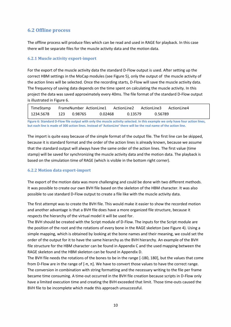
For the export of the muscle activity data the standard D-Flow output is used. After setting up the
correct HBM settings in the MoCap modules (see Figure 5), only the output of the muscle activity of
the action lines will be selected. Once the recording starts, D-Flow will save the muscle activity data.
The frequency of saving data depends on the time spent on calculating the muscle activity. In this
project the data was saved approximately every 40ms. The file format of the standard D-Flow output
is illustrated in Figure 6.
The import is quite easy because of the simple format of the output file. The first line can be skipped,
because it is standard format and the order of the action lines is already known, because we assume
that the standard output will always have the same order of the action lines. The first value (time
stamp) will be saved for synchronizing the muscle activity data and the motion data. The playback is
based on the simulation time of RAGE (which is visible in the bottom right corner).
6.2.2 Motion data export-import
The export of the motion data was more challenging and could be done with two different methods.
It was possible to create our own BVH file based on the skeleton of the HBM character. It was also
possible to use standard D-Flow output to create a file like with the muscle activity data.
The first attempt was to create the BVH file. This would make it easier to show the recorded motion
and another advantage is that a BVH file does have a more organized file structure, because it
respects the hierarchy of the virtual model it will be used for.
The BVH should be created with the Script module of D-Flow. The inputs for the Script module are
the position of the root and the rotations of every bone in the RAGE skeleton (see Figure 4). Using a
simple mapping, which is obtained by looking at the bone names and their meaning, we could set the
order of the output for it to have the same hierarchy as the BVH hierarchy. An example of the BVH
file structure for the HBM character can be found in Appendix C and the used mapping between the
RAGE skeleton and the HBM skeleton can be found in Appendix D.
The BVH file needs the rotations of the bones to be in the range [-180, 180], but the values that come
from D-Flow are in the range of [-π, π]. We have to convert those values to have the correct range.
The conversion in combination with string formatting and the necessary writing to the file per frame
became time consuming. A time-out occurred in the BVH file creation because scripts in D-Flow only
have a limited execution time and creating the BVH exceeded that limit. Those time-outs caused the
BVH file to be incomplete which made this approach unsuccessful.
Figure 6: Standard D-Flow file output with only the muscle activity selected. In this example we only have four action lines, but each line is made of 300 action lines. Instead of ‘ActionLine’ there will be the real name of the action line.
TimeStamp FrameNumber ActionLine1 ActionLine2 ActionLine3 ActionLine4
1234.5678 123 0.98765 0.02468 0.13579 0.56789

11
Without the BVH possibility there still is the MoCap module (for settings see Figure 5) that will result
in a standard D-Flow output file that can be used (see Figure 7). This output will have the rotation
values in the range of [-π, π]. While this was a problem with the BVH file, it no longer is a problem
when we read the file and make quaternions for the rotations. Because of some standard functions
the quaternions are created with the values being in the range [-π, π] and the only thing we need to
worry about is that the correct rotation is applied to the corresponding axis.
Because the motion data is not recorded at the same rate as the muscle activity data (motion data
was recorded approximately once every 10ms and the muscle activity data was recorded
approximately once every 40ms), the playback for both types of data will have a different speed if we
just use the next row of data and it will not be synchronized. Therefore the time stamp is used to
synchronize both data types. The playback is based on the simulation time of RAGE (which is visible
in the bottom right corner).
6.3 Online process
The online process is quite straight forward. A connection between D-Flow and RAGE has to be made
and the data has to be transferred from D-Flow to RAGE where the data will be processed.
The first step is the connection that has to be made. In D-Flow the Script module is used and the
LuaSocket extension made its introduction here. Due to the fact that the script is executed every
frame D-Flow could not hold a steady reliable connection but had to create a connection every time
the script is executed. If there was no disconnection in between the executions, there was a problem
at the client side (RAGE). D-Flow would keep sending data and could not erase previous data that
was transmitted to the socket and RAGE would use old data. With the approach of reconnecting
every time it is ensured that the data is always the newest data.
The script will make D-Flow the server and RAGE will become the client. D-Flow will wait for a client
to present itself. Once there is a client we will send the data to the client. The first values are the
muscle activity data and those values are followed by the root position and then the bone rotations.
The assumption here is that the values are always in the same order and this assumption makes it
possible to use the lookup tables for the muscle coloring that are created at the startup of RAGE.
In RAGE the client was implemented using Boost [6], which was available in RAGE. Because the
length for reading is fixed, it has to be ensured that everything is read and no errors will occur
because it has read too much. To ensure no errors and no lost values, the data that D-Flow is sending
has to be formatted. By limiting the length of the string for the values it can be ensured that a fixed
length for the data will be transmitted. Positive values will have 4 decimals and negative values will
have 3 decimals, because the negative values have to incorporate the minus token which will take up
Figure 7: Standard D-Flow file output with only the root position and every bone rotation selected. In this example we only have the root position and one bone with its orientation, but with multiple bones the rotations will be added at the end of a row.
TimeStamp FrameNumber pos.X pos.Y pos.Z rotation1.X rotation1.Y rotation1.Z
1234.5678 123 0.5 1.5 -0.2 0.56789 -1.23458 0.98765
12
one character of the string. While limiting the number of decimals, there is still enough precision left
for the purpose of this project. Although 3 or 4 decimals is a low resolution for muscle activity, it
does not matter in this project because the difference is not visible in the muscle color or the graph
that is plotted. If a higher precision of the values is necessary, for example for using physics-based
animation, the precision can be enhanced by increasing the length of the reading sequence in the
C++ code and increasing the number of decimals in the D-Flow script.
Once the data is in RAGE it can be used to do the same as has been done with the offline process.
The motion data will be used to show the motion by setting the orientation of the bones and
adjusting the position of the root. The muscle activity data will be used to visualize the muscle
activity in several ways.
6.4 Visualization of the muscle activity
Once the data of the muscle activity is obtained, it is possible to visualize that data. In this project
there are three different approaches. There are materials in the HBM character which can be
colored, a table is available to show the activity and there is the possibility to show the activity in a
graph.
6.4.1 Muscle coloring
One approach to visualize the muscle activity data is by adjusting the color of the muscles to show
how active a muscle is. Unfortunately, the data that D-Flow provides are the activities of the action
lines and not that of the muscles. Luckily, D-Flow has a file that contains the mapping from action
lines to the materials. The mapping of the materials of the virtual character and the action lines is
based on the location in human anatomy and the meaning of their names. After going through the
mapping file it became clear that the file was bigger than necessary for this project. Only the
materials that are depending on action lines are necessary because those are the ones that have to
change color depending on the activity of the action lines. The other materials are for bones and the
muscles that do not have their activity calculated and those materials are not needed because their
color does not have to change.
The result of the smaller mapping file is shown in Appendix A and it contains the material name
which is used in the HBM character and then it shows the names of the action lines that have
influence on the material.
Now knowing what action lines influence the different muscles it is possible to calculate the average
activity. In this project every action line has the same weight. Depending on the average activity the
color of the material of the muscle is changed. If the muscle is active it will be green by default and if
it is non-active it will have its original color red by default. It is possible to change the color of the
active muscle using the sliders in the interface and if the non-active muscles color needs to be
changed, it can be adjusted in the C++ code (but this will only change the color of the muscles that
are depending on action lines and not the color of the muscles whose activity is not calculated in D-
Flow). The interpolation for the material color is linear, which is good enough and it is very cheap
when it needs to be calculated.

13
With the use of some OGRE functions [7] we can access all the materials and adjust only the diffuse
color. This advantage for changing the material instead making new materials is of course memory
usage but it is also an advantage for the computation time.
By now the HBM character will have his muscles colored based on the activity of his muscles. The
advantage for this visualization is that it is a very intuitive type of feedback. When a muscle is turning
green you know that you are activating that muscle during a certain motion. Also when this is used in
the online process you can feel your muscle being active and see how active the muscle is during the
motion.
6.4.2 Table overview
Another approach for the visualization of the muscle activity data is just showing the data in a simple
table. The table consists of two columns and 300 rows (one for each action line). The first column
contains the name of the action line and the second column contains the value of the activity of the
action line.
The table shows the value of each action line and will be updated every frame. The advantage for this
visualization is that you can look for specific action lines and see what the activity of that action line
is. The disadvantage for this approach is that you see a lot of data because it changes its values really
fast and you will not be able to interpret this data well at that speed. If the activity data from the
playback needs a closer look, it can be analyzed reading the standard D-Flow file that is loaded into
RAGE.
6.4.3 Plotting
The third approach for visualization is to plot a graph with the muscle activity (see Figure 8). For the
plotting the Python plotting library mathplotlib [8] is used. This library came with the files for RAGE
but has to be installed along with Python itself. There is also the numpy library which is used by the
mathplotlib and also has to be installed.
The x-axis on the graph is the time and it is counted in the number of frames since the plotting
began. On the y-axis the muscle activity is represented and will show values between 0 and 1.
There are 8 different colors that can be used and a variety of markers can make the lines distinctive.
A total of 15 action lines can be monitored using the graph plotting. Adding an action line to the
graph can be done by clicking the action line in the table overview.
It is also possible to adjust the number of points per action line that has to be plotted. This has
several advantages. By increasing the amount of points to plot, it is possible to monitor the action
lines for a longer amount of time. By decreasing the amount of points you can accelerate the frame
rate because the plotting can take a lot of processing power and will decrease the frame rate. This
means of course that it is hardware dependent and it is a good idea to keep the amount of points to
plot low on a slower system.

14
Figure 8: Example of the graph in its separate window. This example shows five action lines with 20 points to plot for every action line.
The main advantage of plotting is already mentioned but it is that it makes it possible to monitor the
activity of an action line over time and compare it with other action lines. This will give an overview
of the activity of an action line during a motion and makes it possible to see connections between
different action lines or different, but maybe similar motions.
6.4.4 Comparison
In my opinion the best approach for the muscle activity at a certain time is the muscle coloring
approach. This seems to be the best approach because while you are performing a motion, you are
immediately seeing what muscles you are using and to some extend how much you use those
muscles. This provides a very intuitive way for a user to see his muscle activity. The table overview is
too complicated for a quick lookup even though it gives the exact muscle activity value. If a game
would be made where you have to use muscle activity it could be useful to use the muscle coloring
for the visualization.
If we need feedback for muscle activity over time then I would think that the plotting option is the
best approach. With this approach you can monitor several action lines and see what happens with
their activity over time. This option could be used when you are analyzing a motion and want to
know what muscles are active during a certain motion and also you can see how active a muscle is
during the motion. If you would like to use the table overview approach you will have a hard time to

15
monitor the several action lines and remember what happened to the activities. The muscle coloring
could also be used for the muscle activity over time, because it is easier to remember a muscle that is
changing color than a number changing its value very fast.
If a best approach has to be chosen then the muscle coloring would be the winner because you can
easily see the activity of several muscles for both a time period and a certain point in time. The
second best approach would be the plotting option because you can compare the different action
lines with each other and monitor them over time. The table overview seems to be quite a useless
approach because it changes its values too fast to see and remember it well. Also with all those
action line names and their values it is too much information to use. For now the table overview
approach is only useful for selecting action lines for plotting.

16
References
1. The programming language Lua,
http://www.lua.org
2. LuaSocket, Network support for the Lua language,
http://w3.impa.br/~diego/software/luasocket
3. A real-time system for biomechanical analysis of human movement and muscle function,
Antonie J. van den Bogert, Thomas Geijtenbeek, Oshri Even-Zohar, Frans Steenbrink,
Elizabeth C. Hardin, Med Biol Eng Comput (2013) 51: 1069-1077,
http://link.springer.com/content/pdf/10.1007%2Fs11517-013-1076-z.pdf
4. OGRE Open Source 3D Graphics Engine,
http://www.ogre3d.org
5. Biovision Hierarchy BVH File format,
http://research.cs.wisc.edu/graphics/Courses/cs-838-1999/Jeff/BVH.html
6. Boost C++ libraries, asio tutorials synchronous TCP client,
http://www.boost.org/doc/libs/1_55_0/doc/html/boost_asio/tutorial/tutdaytime1/src.html
7. OGRE3D materials tutorial,
http://www.ogre3d.org/tikiwiki/tiki-
index.php?page=MadMarx+Tutorial+7&structure=Tutorials
8. Mathplotlib python plotting library,
http://matplotlib.org/

17
Appendix
A. Action lines belonging to HBM character materials The first name is the material (starting with ‘muscle_mat’) and the names that follow are the
action lines that have influence on the material.
muscle_mat_l_adductor_brevis L_AdductorBrevis
muscle_mat_l_adductor_longus L_AdductorLongus
muscle_mat_l_adductor_magnus L_AdductorMagnus1 L_AdductorMagnus2 L_AdductorMagnus3
muscle_mat_l_biceps_brachii L_BicepsBrachiiLH L_BicepsBrachiiSH1 L_BicepsBrachiiSH2
muscle_mat_l_biceps_femoris L_BicepsFemorisLH L_BicepsFemorisSH
muscle_mat_l_brachialis L_Brachialis1 L_Brachialis2 L_Brachialis3 L_Brachialis4 L_Brachialis5 L_Brachialis6 L_Brachialis7
muscle_mat_l_brachioradialis L_Brachioradialis1 L_Brachioradialis2 L_Brachioradialis3
muscle_mat_l_deltoid L_DeltoidClavicular1 L_DeltoidClavicular2 L_DeltoidClavicular3 L_DeltoidClavicular4 L_DeltoidScapular10 L_DeltoidScapular11
L_DeltoidScapular1 L_DeltoidScapular2 L_DeltoidScapular3 L_DeltoidScapular5 L_DeltoidScapular6 L_DeltoidScapular7 L_DeltoidScapular8 L_DeltoidScapular9
muscle_mat_l_extensor_digitorum_longus L_ExtensorDigLongus
muscle_mat_l_extensor_hallucis_longus L_ExtensorHalLongus
muscle_mat_l_external_obliques1 L_ObliqueExternal
muscle_mat_l_flexor_digitorum_longus L_FlexDigLongus
muscle_mat_l_flexor_hallucis_longus L_FlexHalLongus
muscle_mat_l_gastrocnemius L_LateralGastroc L_MedialGastroc
muscle_mat_l_gluteus_maximus L_GluteusMaximus1 L_GluteusMaximus2 L_GluteusMaximus3
muscle_mat_l_gluteus_medius L_GluteusMedius1 L_GluteusMedius2 L_GluteusMedius3
muscle_mat_l_gluteus_minimus L_GluteusMinimus1 L_GluteusMinimus2 L_GluteusMinimus3
muscle_mat_l_gracilis L_Gracilis
muscle_mat_l_iliocostalis_cervicis L_ErectorSpinae
muscle_mat_l_iliocostalis_lumborum L_ErectorSpinae
muscle_mat_l_iliocostalis_thoracis L_ErectorSpinae
muscle_mat_l_iliospoas L_Iliacus L_Psoas
muscle_mat_l_infraspinatus L_Infraspinatus1 L_Infraspinatus2 L_Infraspinatus3 L_Infraspinatus4 L_Infraspinatus5 L_Infraspinatus6
muscle_mat_l_interspinalis L_ErectorSpinae
muscle_mat_l_latissimus_dorsi L_LatissimusDorsi1 L_LatissimusDorsi2 L_LatissimusDorsi3 L_LatissimusDorsi4 L_LatissimusDorsi5 L_LatissimusDorsi6
muscle_mat_l_longissimus_capitis L_ErectorSpinae
muscle_mat_l_longissimus_cervicis L_ErectorSpinae
muscle_mat_l_longissimus_thoracis L_ErectorSpinae
muscle_mat_l_obliquus_capitis_inferior L_ObliqueInternal
muscle_mat_l_obliquus_capitis_superior L_ObliqueInternal
muscle_mat_l_pectineus L_Pectineus
muscle_mat_l_pectoralis_major L_PectoralisMajorCH1 L_PectoralisMajorCH2 L_PectoralisMajorTH1 L_PectoralisMajorTH2 L_PectoralisMajorTH3
L_PectoralisMajorTH4 L_PectoralisMajorTH5 L_PectoralisMajorTH6
muscle_mat_l_peroneus_brevis L_PeroneusBrevis
muscle_mat_l_peroneus_longus L_PeroneusTertius
muscle_mat_l_piriformis L_Piriformis
muscle_mat_l_quadratus_femoris L_QuadratusFemoris
muscle_mat_l_quadratus_lumborum L_QuadratusLumborum
muscle_mat_l_rectus_abdominus L_RectusAbdominis
muscle_mat_l_rectus_femoris L_RectusFemoris
muscle_mat_l_rotatores L_ErectorSpinae
muscle_mat_l_sartorius L_Sartorius
muscle_mat_l_semimembranosus L_Semimembranosus
muscle_mat_l_semispinalis_capitis L_ErectorSpinae
muscle_mat_l_semispinalis_cervicis L_ErectorSpinae
muscle_mat_l_semispinalis_thoracics L_ErectorSpinae
muscle_mat_l_semitendinosus L_Semitendinosus
muscle_mat_l_soleus L_Soleus
muscle_mat_l_spinalis_thoracis L_ErectorSpinae
muscle_mat_l_splenius_capitis L_ErectorSpinae
muscle_mat_l_splenius_cervicis L_ErectorSpinae
muscle_mat_l_superior_gemellus L_Gemelli
muscle_mat_l_tensor_fascia_latae L_TensorFasciaLata
muscle_mat_l_teres_major L_TeresMajor1 L_TeresMajor2 L_TeresMajor3 L_TeresMajor4
muscle_mat_l_tibialis_anterior L_TibialisAnterior
muscle_mat_l_tibialis_posterior L_TibialisPosterior
muscle_mat_l_triceps_brachii L_TricepsLH1 L_TricepsLH2 L_TricepsLH3 L_TricepsLH4 L_TricepsLatH1 L_TricepsLatH2 L_TricepsLatH3 L_TricepsLatH4 L_TricepsLatH5
L_TricepsMedH1 L_TricepsMedH2 L_TricepsMedH3 L_TricepsMedH4 L_TricepsMedH5

18
muscle_mat_l_vastus_intermedius L_VastusIntermedius
muscle_mat_l_vastus_lateralis L_VastusLateralis
muscle_mat_l_vastus_medialis L_VastusMedialis
muscle_mat_r_adductor_brevis R_AdductorBrevis
muscle_mat_r_adductor_longus R_AdductorLongus
muscle_mat_r_adductor_magnus R_AdductorMagnus1 R_AdductorMagnus2 R_AdductorMagnus3
muscle_mat_r_biceps_brachii R_BicepsBrachiiSH1 R_BicepsBrachiiSH2
muscle_mat_r_biceps_femoris R_BicepsFemorisLH R_BicepsFemorisSH
muscle_mat_r_brachialis R_Brachialis1 R_Brachialis2 R_Brachialis3 R_Brachialis4 R_Brachialis5 R_Brachialis6 R_Brachialis7
muscle_mat_r_brachioradialis R_Brachioradialis1 R_Brachioradialis2 R_Brachioradialis3
muscle_mat_r_deltoid R_DeltoidClavicular1 R_DeltoidClavicular2 R_DeltoidClavicular3 R_DeltoidClavicular4 R_DeltoidScapular10 R_DeltoidScapular11
R_DeltoidScapular1 R_DeltoidScapular2 R_DeltoidScapular3 R_DeltoidScapular5 R_DeltoidScapular6 R_DeltoidScapular7 R_DeltoidScapular8 R_DeltoidScapular9
muscle_mat_r_extensor_digitorum_longus R_ExtensorDigLongus
muscle_mat_r_extensor_hallucis_longus R_ExtensorHalLongus
muscle_mat_r_external_obliques1 R_ObliqueExternal
muscle_mat_r_flexor_digitorum_longus R_FlexDigLongus
muscle_mat_r_flexor_hallucis_longus R_FlexHalLongus
muscle_mat_r_gastrocnemius R_LateralGastroc R_MedialGastroc
muscle_mat_r_gluteus_maximus R_GluteusMaximus1 R_GluteusMaximus2 R_GluteusMaximus3
muscle_mat_r_gluteus_medius R_GluteusMedius1 R_GluteusMedius2 R_GluteusMedius3
muscle_mat_r_gluteus_minimus R_GluteusMinimus1 R_GluteusMinimus2 R_GluteusMinimus3
muscle_mat_r_gracilis R_Gracilis
muscle_mat_r_iliocostalis_cervicis R_ErectorSpinae
muscle_mat_r_iliocostalis_lumborum R_ErectorSpinae
muscle_mat_r_iliocostalis_thoracis R_ErectorSpinae
muscle_mat_r_iliospoas R_Iliacus R_Psoas
muscle_mat_r_infraspinatus R_Infraspinatus1 R_Infraspinatus2 R_Infraspinatus3 R_Infraspinatus4 R_Infraspinatus5 R_Infraspinatus6
muscle_mat_r_interspinalis R_ErectorSpinae
muscle_mat_r_latissimus_dorsi R_LatissimusDorsi1 R_LatissimusDorsi2 R_LatissimusDorsi3 R_LatissimusDorsi4 R_LatissimusDorsi6
muscle_mat_r_longissimus_capitis R_ErectorSpinae
muscle_mat_r_longissimus_cervicis R_ErectorSpinae
muscle_mat_r_longissimus_thoracis R_ErectorSpinae
muscle_mat_r_obliquus_capitis_inferior R_ObliqueInternal
muscle_mat_r_obliquus_capitis_superior R_ObliqueInternal
muscle_mat_r_pectineus R_Pectineus
muscle_mat_r_pectoralis_major R_PectoralisMajorCH1 R_PectoralisMajorCH2 R_PectoralisMajorTH1 R_PectoralisMajorTH2 R_PectoralisMajorTH3
R_PectoralisMajorTH4 R_PectoralisMajorTH5 R_PectoralisMajorTH6
muscle_mat_r_peroneus_brevis R_PeroneusBrevis
muscle_mat_r_peroneus_longus R_PeroneusLongus
muscle_mat_r_peroneus_tertius R_PeroneusTertius
muscle_mat_r_piriformis R_Piriformis
muscle_mat_r_quadratus_femoris R_QuadratusFemoris
muscle_mat_r_quadratus_lumborum R_QuadratusLumborum
muscle_mat_r_rectus_abdominus R_RectusAbdominis
muscle_mat_r_rectus_femoris R_RectusFemoris
muscle_mat_r_rotatores R_ErectorSpinae
muscle_mat_r_sartorius R_Sartorius
muscle_mat_r_semimembranosus R_Semimembranosus
muscle_mat_r_semispinalis_capitis R_ErectorSpinae
muscle_mat_r_semispinalis_cervicis R_ErectorSpinae
muscle_mat_r_semispinalis_thoracics R_ErectorSpinae
muscle_mat_r_semitendinosus R_Semitendinosus
muscle_mat_r_soleus R_Soleus
muscle_mat_r_spinalis_thoracis R_ErectorSpinae
muscle_mat_r_splenius_capitis R_ErectorSpinae
muscle_mat_r_splenius_cervicis R_ErectorSpinae
muscle_mat_r_superior_gemellus R_Gemelli
muscle_mat_r_tensor_fascia_latae R_TensorFasciaLata
muscle_mat_r_teres_major R_TeresMajor1 R_TeresMajor2 R_TeresMajor3 R_TeresMajor4
muscle_mat_r_teres_minor R_TeresMinor1 R_TeresMinor2 R_TeresMinor3
muscle_mat_r_tibialis_anterior R_TibialisAnterior
muscle_mat_r_tibialis_posterior R_TibialisPosterior
muscle_mat_r_triceps_brachii R_TricepsLH1 R_TricepsLH2 R_TricepsLH3 R_TricepsLH4 R_TricepsLatH1 R_TricepsLatH2 R_TricepsLatH3 R_TricepsLatH4
R_TricepsLatH5 R_TricepsMedH1 R_TricepsMedH2 R_TricepsMedH3 R_TricepsMedH4 R_TricepsMedH5
muscle_mat_r_vastus_intermedius R_VastusIntermedius
muscle_mat_r_vastus_lateralis R_VastusLateralis
muscle_mat_r_vastus_medialis R_VastusMedialis

19
B. Listing of the action lines Using the standard D-Flow order for the action lines gives the following listing which is used
for representation in the table overview and used in the several lookup tables.
R_GluteusMedius1 R_GluteusMedius2 R_GluteusMedius3 R_GluteusMinimus1 R_GluteusMinimus2
R_GluteusMinimus3 R_Semimembranosus R_Semitendinosus R_BicepsFemorisLH R_Sartorius R_AdductorLongus
R_AdductorBrevis R_AdductorMagnus1 R_AdductorMagnus2 R_AdductorMagnus3 R_TensorFasciaLata
R_Pectineus R_Gracilis R_GluteusMaximus1 R_GluteusMaximus2 R_GluteusMaximus3 R_Iliacus R_Psoas
R_QuadratusFemoris R_Gemelli R_Piriformis R_RectusFemoris R_BicepsFemorisSH R_VastusMedialis
R_VastusIntermedius R_VastusLateralis R_MedialGastroc R_LateralGastroc R_Soleus R_TibialisPosterior
R_FlexDigLongus R_FlexHalLongus R_TibialisAnterior R_PeroneusBrevis R_PeroneusLongus
R_PeroneusTertius R_ExtensorDigLongus R_ExtensorHalLongus L_GluteusMedius1 L_GluteusMedius2
L_GluteusMedius3 L_GluteusMinimus1 L_GluteusMinimus2 L_GluteusMinimus3 L_Semimembranosus
L_Semitendinosus L_BicepsFemorisLH L_Sartorius L_AdductorLongus L_AdductorBrevis
L_AdductorMagnus1 L_AdductorMagnus2 L_AdductorMagnus3 L_TensorFasciaLata L_Pectineus L_Gracilis
L_GluteusMaximus1 L_GluteusMaximus2 L_GluteusMaximus3 L_Iliacus L_Psoas L_QuadratusFemoris
L_Gemelli L_Piriformis L_RectusFemoris L_BicepsFemorisSH L_VastusMedialis L_VastusIntermedius
L_VastusLateralis L_MedialGastroc L_LateralGastroc L_Soleus L_TibialisPosterior L_FlexDigLongus
L_FlexHalLongus L_TibialisAnterior L_PeroneusBrevis L_PeroneusLongus L_PeroneusTertius
L_ExtensorDigLongus L_ExtensorHalLongus R_DeltoidScapular1 R_DeltoidScapular2 R_DeltoidScapular3
R_DeltoidScapular4 R_DeltoidScapular5 R_DeltoidScapular6 R_DeltoidScapular7 R_DeltoidScapular8
R_DeltoidScapular9 R_DeltoidScapular10 R_DeltoidScapular11 R_DeltoidClavicular1 R_DeltoidClavicular2
R_DeltoidClavicular3 R_DeltoidClavicular4 R_CoracoBrachialis1 R_CoracoBrachialis2 R_CoracoBrachialis3
R_Infraspinatus1 R_Infraspinatus2 R_Infraspinatus3 R_Infraspinatus4 R_Infraspinatus5
R_Infraspinatus6 R_TeresMinor1 R_TeresMinor2 R_TeresMinor3 R_TeresMajor1
R_TeresMajor2 R_TeresMajor3 R_TeresMajor4 R_Supraspinatus1 R_Supraspinatus2
R_Supraspinatus3 R_Supraspinatus4 R_Subscapularis1 R_Subscapularis2 R_Subscapularis3
R_Subscapularis4 R_Subscapularis5 R_Subscapularis6 R_Subscapularis7 R_Subscapularis8
R_Subscapularis9 R_Subscapularis10 R_Subscapularis11 R_BicepsBrachiiLH R_BicepsBrachiiSH1
R_BicepsBrachiiSH2 R_TricepsLH1 R_TricepsLH2 R_TricepsLH3 R_TricepsLH4
R_LatissimusDorsi1 R_LatissimusDorsi2 R_LatissimusDorsi3 R_LatissimusDorsi4 R_LatissimusDorsi5
R_LatissimusDorsi6 R_PectoralisMajorTH1 R_PectoralisMajorTH2 R_PectoralisMajorTH3 R_PectoralisMajorTH4
R_PectoralisMajorTH5 R_PectoralisMajorTH6 R_PectoralisMajorCH1 R_PectoralisMajorCH2 R_TricepsMedH1
R_TricepsMedH2 R_TricepsMedH3 R_TricepsMedH4 R_TricepsMedH5 R_Brachialis1
R_Brachialis2 R_Brachialis3 R_Brachialis4 R_Brachialis5 R_Brachialis6
R_Brachialis7 R_Brachioradialis1 R_Brachioradialis2 R_Brachioradialis3 R_PronatorTeres1
R_PronatorTeres2 R_Supinator1 R_Supinator2 R_Supinator3 R_Supinator4
R_Supinator5 R_PronatorQuadratus1 R_PronatorQuadratus2 R_PronatorQuadratus3 R_TricepsLatH1
R_TricepsLatH2 R_TricepsLatH3 R_TricepsLatH4 R_TricepsLatH5 R_Anconeus1
R_Anconeus2 R_Anconeus3 R_Anconeus4 R_Anconeus5 L_DeltoidScapular1
L_DeltoidScapular2 L_DeltoidScapular3 L_DeltoidScapular4 L_DeltoidScapular5 L_DeltoidScapular6
L_DeltoidScapular7 L_DeltoidScapular8 L_DeltoidScapular9 L_DeltoidScapular10 L_DeltoidScapular11
L_DeltoidClavicular1 L_DeltoidClavicular2 L_DeltoidClavicular3 L_DeltoidClavicular4 L_CoracoBrachialis1
L_CoracoBrachialis2 L_CoracoBrachialis3 L_Infraspinatus1 L_Infraspinatus2 L_Infraspinatus3
L_Infraspinatus4 L_Infraspinatus5 L_Infraspinatus6 L_TeresMinor1 L_TeresMinor2
L_TeresMinor3 L_TeresMajor1 L_TeresMajor2 L_TeresMajor3 L_TeresMajor4
L_Supraspinatus1 L_Supraspinatus2 L_Supraspinatus3 L_Supraspinatus4 L_Subscapularis1
L_Subscapularis2 L_Subscapularis3 L_Subscapularis4 L_Subscapularis5 L_Subscapularis6
L_Subscapularis7 L_Subscapularis8 L_Subscapularis9 L_Subscapularis10 L_Subscapularis11
L_BicepsBrachiiLH L_BicepsBrachiiSH1 L_BicepsBrachiiSH2 L_TricepsLH1 L_TricepsLH2
L_TricepsLH3 L_TricepsLH4 L_LatissimusDorsi1 L_LatissimusDorsi2 L_LatissimusDorsi3
L_LatissimusDorsi4 L_LatissimusDorsi5 L_LatissimusDorsi6 L_PectoralisMajorTH1 L_PectoralisMajorTH2
L_PectoralisMajorTH3 L_PectoralisMajorTH4 L_PectoralisMajorTH5 L_PectoralisMajorTH6 L_PectoralisMajorCH1
L_PectoralisMajorCH2 L_TricepsMedH1 L_TricepsMedH2 L_TricepsMedH3 L_TricepsMedH4
L_TricepsMedH5 L_Brachialis1 L_Brachialis2 L_Brachialis3 L_Brachialis4
L_Brachialis5 L_Brachialis6 L_Brachialis7 L_Brachioradialis1 L_Brachioradialis2
L_Brachioradialis3 L_PronatorTeres1 L_PronatorTeres2 L_Supinator1 L_Supinator2
L_Supinator3 L_Supinator4 L_Supinator5 L_PronatorQuadratus1 L_PronatorQuadratus2
L_PronatorQuadratus3 L_TricepsLatH1 L_TricepsLatH2 L_TricepsLatH3 L_TricepsLatH4
L_TricepsLatH5 L_Anconeus1 L_Anconeus2 L_Anconeus3 L_Anconeus4
L_Anconeus5 L_ErectorSpinae R_ErectorSpinae L_ObliqueExternal R_ObliqueExternal
L_ObliqueInternal R_ObliqueInternal L_QuadratusLumborum R_QuadratusLumborum L_RectusAbdominis
R_RectusAbdominis

20
C. BVH file structure An example of the BVH file structure that can be used for the motion of the HBM character.
HIERARCHY
ROOT pelvis
{
OFFSET 0 0 0
CHANNELS 6 Xposition Yposition Zposition Xrotation Yrotation Zrotation
JOINT thorax
{
OFFSET 0 0 0
CHANNELS 3 Xrotation Yrotation Zrotation
JOINT spine
{
OFFSET 0 0 0
CHANNELS 3 Xrotation Yrotation Zrotation
JOINT hbm_spine_null
{
OFFSET 0 0 0
CHANNELS 3 Xrotation Yrotation Zrotation
JOINT neck
{
OFFSET 0 0 0
CHANNELS 3 Xrotation Yrotation Zrotation
JOINT head
{
OFFSET 0 0 0
CHANNELS 3 Xrotation Yrotation Zrotation
End Site
{
OFFSET 0 0 0
} } }
JOINT rclavicle
{
OFFSET 0 0 0
CHANNELS 3 Xrotation Yrotation Zrotation
JOINT rhumerus
{
OFFSET 0 0 0
CHANNELS 3 Xrotation Yrotation Zrotation
JOINT rradius
{
OFFSET 0 0 0
CHANNELS 3 Xrotation Yrotation Zrotation
JOINT rhand
{
OFFSET 0 0 0
CHANNELS 3 Xrotation Yrotation Zrotation
End Site
{
OFFSET 0 0 0
} } } } }
JOINT lclavicle
{
% same as the right part
} } } }
JOINT pelvislegs
{
OFFSET 0 0 0
CHANNELS 3 Xrotation Yrotation Zrotation
JOINT rfemur
{
OFFSET 0 0 0
CHANNELS 3 Xrotation Yrotation Zrotation
JOINT rtibia
{
OFFSET 0 0 0
CHANNELS 3 Xrotation Yrotation Zrotation
JOINT rfoot
{
OFFSET 0 0 0
CHANNELS 3 Xrotation Yrotation Zrotation
JOINT rtoes
{
OFFSET 0 0 0
CHANNELS 3 Xrotation Yrotation Zrotation
End Site
{
OFFSET 0 0 0
} } } } }
JOINT lfemur
{
% same as the right part
} } }
MOTION
Frames: % number of frames
Frame Time: %frame time

21
D. Mapping from RAGE skeleton to HBM skeleton The mapping from the RAGE skeleton to the HBM skeleton that is used to animate the
correct bones in the HBM character. The mapping is found by looking at the names of the
bones and their meaning.
RAGE Performance skeleton bone HBM character bone
root pelvis
r_hip rfemur
r_knee rtibia
r_ankle rfoot
r_subtalar rtoes
l_hip lfemur
l_knee ltibia
l_ankle lfoot
l_subtalar ltoes
vl5 thorax
vl1 spine
vt10 hbm_spine_null
vt1 neck
vc2 head
r_sternoclavicular rclavicle
r_shoulder rhumerus
r_elbow rradius
r_wrist rhand
l_sternoclavicular lclavicle
l_shoulder lhumerus
l_elbow lradius
l_wrist lhand