N93- 71674 i47

DESIGN OF OPTIMUM DUCTS USING AN

EFFICIENT 3-D VISCOUS COMPUTATIONAL FLOW ANALYSIS

Ravl K. Madabhushl

Ralph LevySteven M. Pincus*

Scientific Research Associates

P.O. Box 1058

Glastonbury, CT 06033

ABSTRACT

Design of fluid dynamically efficient ducts is addressed through the

combination of an optimization analysis with a three-dlmenslonal viscous fluid

dynamic analysis code. For efficiency, a parabolic fluid dynamic analysis was

used. Since each function evaluation _n an optimization analysis is a full

three-dlmenslonal viscous flow analysis requiring 200,000 grid points, it is

important to use both an efficient fluid dynamic analysis and an efficient

optimization technique. Three optimization techniques are evaluated on a

series of test functions. The Quasi-Newton (BFGS, _ = .9) technique was

selected as the preferred technique. A series of basic duct design problems

are performed. On a two-parameter optimization problem, the BFGS technique is

demonstrated to require half as many function evaluations as a steepest descent

technique.

INTRODUCTION

The subject study combines an existing, well-proven, three-dlmenslonal,

viscous duct flow analysis with a formal optimization procedure to design a

duct that is optimum for a given application. The fluid dynamics code used in

this effort is a three-dlmensional, viscous flow, forward marching calculation

developed by Scientific Research Associates under ONR and NASA Lewis Research

Center Contract support. This analysis solves a set of fluid flow equations

*Present address: AVCO, Stratford, CT

https://ntrs.nasa.gov/search.jsp?R=19930074227 2020-06-02T06:34:40+00:00Z

148

that are parabolic in the predominant flow direction. Physical approximationsare madeto the Navier-Stokes equations resulting in an analysis that is much

faster to use by a factor of I0 to I00 than the full Navier-Stokes equations

for flows which have an _ priori specifiable predominant flow direction, such

as duct flows. The capability of this analysis has been clearly demonstrated

by Levy, Briley and McDonald (Ref. I) and by Towne (Ref. 2). These references

document application of this analysis to a wide variety of viscous flow duct

'S' bends circularproblems with configurations such as 90 ° bends, 180 ° bends,

to square cross-section, etc. In all cases, comparison with existing high

quality experimental data was shown to be very good.

In its original form, this parabolic flow analysis provides a powerful

tool for analyzing three-dlmensional, viscous flow in ducts. However, the

engineering design problem is the design of ducts for a specific application

subject to specified constraints. The subject study initiated a program to

combine the viscous flow analysis with an optimization procedure to design such

ducts.

Development of this design procedure will give the aerospace and

hydrodynamic design and development community a powerful new tool to aid in the

design of fluid dynamic components. Such a tool would automate the duct design

procedure. Currently, ducts are designed through _ series of calculations and

tests which are performed until a duct is obtained which meets certain design

criteria. The current process does not ensure an orderly progression toward a

best design and indeed does not even ensure the final design is optimum in any

sense. The subject study could provide a tool of validated accu=acy that would

quickly and accurately design a duct within engineering (user-specified)

constraints that is the optimum for the specific application.

Since each function evaluation in an optimization process is a

three-dimensional viscous flow clculation requiring 200,000 grid points, it is

important to use efficient optimization technqiues. Three optimization

techniques are evaluated on a series of ten test functions to determine an

optimization technique Judged best for the type of probelms encountered in duct

flow analysis. These are presented in the following section.

149

OPTIMIZATION

Modelling the performance of a physical system by an objective function

meansassociating a real numberwith each set of system independent variables.

This objective function gives a single measureof "goodness" of the system for

the given values of the variables. The task of optimizing is finding the value

and location of the minimumof the objective function. The discussion of

optimization techniques which follows is practical for problems with a smallnumberof variables (less than 200).

For the subject application, the objective function is highly non-linear

and requires solving a coupled system of partial differential equations toevaluate the function value at a given point (set of independent variable

values). Objective function evaluations can be very expensive comparedto any

other calculations needed for each of the optimization methods considered. One

optimization methodwill be Judgedbetter than another if it consistently needs

fewer objective function evaluations to achieve a desired level of accuracy,since it would cost less to use the better optimization to achieve that

accuracy. The general form of an optimization problem is

minimize F(x)xERn

subject to ci(x)-0 ,

cj(x)>0,

The objective function is F(x), and the constraints are given by the c's where

x is a vector of independent variables of the system.

Search Direction

Several types of iterative search methods were investigated. They all

have the following form in common. At the start of the k-th iterations, xk

is the current estimate of the minimum. The k-th iteration then consists of

the computation of a search vector, Pk, from which the new estimate, Xk+l,

is found from:

Xk+ I = xk + akp k (I)

150

where _k is obtained by one-dimenslonal search. The methods studied ultimatelystem from the central notion from calculus of the descent direction. The

calculus theorem states that at a given point the local direction of steepestdescent is in the direction that is opposite to the gradient. In Eq. (I) one

could compute the gradient at Xk, denoted as gk, and let pkI -gk; then for

suitably small _k' somefunction reduction would be guaranteed; that is,

Fk+1 < Fk, where Fk - F(Xk). This choice of Pk defines GRAD,the gradientmethod, also knownas the steepest descent method.

In these methods, one must estimate the gradient at each starting point of

a one-dlmensional search. Using the first order approximation in a Taylor

expansion about the starting point, this involves 'n' function evaluations per

linear search, where n is the numberof independent variables underconsideration. To include second order behavior, one can choose either to

directly compute the Hessian matrix of second derivatives by finite

differences, or to somehow approximate it from previous information. Direct

evaluation of the Hessian matrix at each one-dlmenslonal starting point would

cost many additional function evaluations, and has long since been rejected by

practitioners. A conjugate gradient method (CG) is designed as a crude but

easily applied approximate quadratic search update. The Quasi-Newton methods

approximate the Hessian matrix by a positive definite matrix for each

one-dlmensional search.

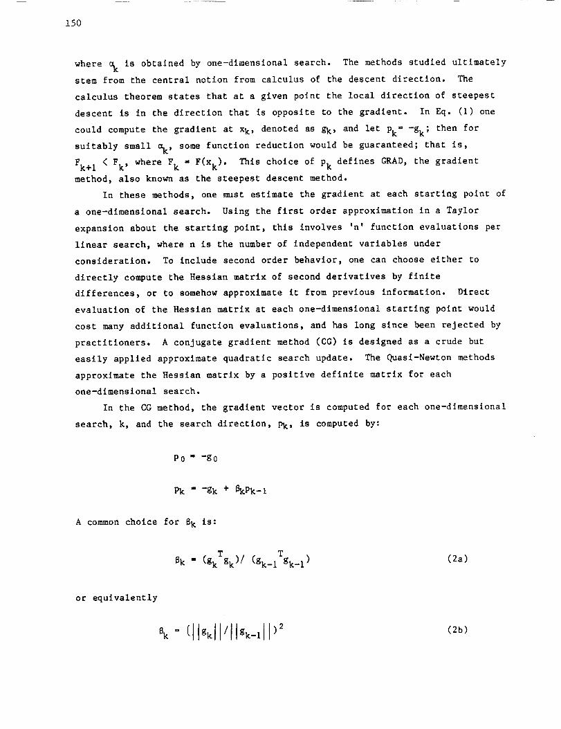
In the CG method, the gradient vector is computed for each one-dlmensional

search, k, and the search direction, Pk, is computed by:

P0 " -go

Pk " -gk + BkPk-i

A common choice for _k is:

Bk - (gkTgk)/ (gk_iTgk_l) (2a)

or equivalently

151

where gT refers to the transpose of the vector g. This algorithm performs

quite a bit better than does GRAD, but it can still be substantially improved

upon by the Quasi-Newton methods. There are two reasons for this. First,

functions with strong coupling between independent variables typically require

many CG direction updates to successfully improve the successive approximations

to the optimum. Second, each of the two gradient methods presented above

require accurate one-dlmenslonal searches to give _ood performance.

Quasi-Newton optimization methods are based on Newton's method, which is

designed to achieve termination (minimum) in a single iteration for a quadratic

function, given the first and second derivatives of the function. Consider an

arbitrary point, Xk, and a vector, Pk' for a quadratic function. The Taylor

series gives the expansion of the gradient at Xk+ 1 = Xk+ Pk as gk+l = g(xk+Pk)

= gk + GPk' since hlgher-order derivative terms are 0. If Xk+ I is to be the

minimum of the function, then gk+l must be 0 and then Pk is given by

Pk = -G- Igk

For non-quadratic functions, one iteration termination will not be

achieved, but a method which accurately estimates G-I should provide an

effective scheme for successive search directions. This logic formed the

intuition behind the Quasi-Newton methods, which were developed in the 1960's

and early 1970's. Until then, the CG method was the most commonly used search

update procedure. In the early 1960's, Davldon, and then Fletcher and Powell

independently came up with a Quasi-Newton method in which, at the k-th

iteration,

Pk = -Hkgk

where Hk is approximated from gradient information. This updating gave

substantial improvement over the gradient methods in that it required many

fewer function evaluations to achieve a given degree of accuracy. In 1970,

several additional authors independently came out out with an improved updating

formula for Hk. The authors were Broyden, Fletcher, Goldfarb and Shanno, and

their formula is known as the BFGS formula.

152

Hk+I = (I- AxkAgkT)AxkTAgk

Hk (I - AxkAgkT)T AXkAXkTAXk T Agk + AXk TAg k

(3)

One-Dimenslonal Search

The objective of the one-dimensional search algorithm is to minimize the

objective function evaluated along the search direction. Assuming that the

function evaluated along this direction is unimodal, three different methods of

performing one-dimensional search were studied: Golden Section, Safeguarded

Quadratic, and Brent's hybrid method. A detailed description of the algorithms

is not presented here because it turned out that the choice of one-dimensional

algorithm made very little difference in the determination of a best

optimization method.

One-Dimensional Termination Criteria

The termination requirement for stopping a given one-dimensional search is

that two reduction criteria are met: a reduction of the objective function and

a specified reduction in the directed gradient

F(Xk+SPk ) -F(Xk) < UspkTg(xk ) , for 0<U<I/2 (4)

Tg(xk+=Pk)l<-npkTg(xk) , where 0<n<l(5)

The choice of _ in Eq. (5) is the parameter that determines the crudeness

of the one-dimensional search; _ near 1 gives a crude search, n near 0 gives a

very accurate one. The tradeoffs are that a crude search requires fewer

function evaluations per linear search, but more directional searches, with the

more accurate searches having the opposite behavior.

Three values of n were chosen in making comparisons, n m.9, .05, and

•001. These values for n represent coarse, fairly accurate, and very accurate

one-dlmenslonal searches. As noted in the literature, and as reinforced in

Table I, the gradient methods require a very small n, typically .001 or

smaller, to be effective. A value of U - .0001 was maintained for Eq. (4).

search results when it is required that IPkTg(xk+sPk)l = 0,An exact linearl m

i.e., that _ = 0. Virtually all of the theoretical investigations of

153

performance of search direction algorithms (BFGS,CG, etc.) require that exactlinear searches be performed. However, as shownin the next section, a very

small value of _ does not give excellent algorithm efficiency in terms offunction evaluations.

Initial Point in One-Dimenslonal Search

In analyzing the performance of alternative algorithms for various test

functions, the choice of starting point for each one-dlmensional search was

crucial. It was found that the consensus in the literature for an initial

choice of ak in Eq. (I) was _k = I. This choice works exactly for quadratic

functions when exact gradient and Hessian information is known for BFGS. In

fact, for BFGS with a course search (_ = .9). this initial point is usually

good that for virtually all of the test functions, after the first few

direction searches, most one-dlmensional searches are terminated after either

one or two function evaluations. _k = I for all k was chosen as the starting

point for all algorithms that are compared below.

Test Functions

Each of the candidate algorithms was tested for a variety of functions.

Five of the functions were taken from the standard literature (Refs. 3-4).

These were functions that many authors used to draw conclusions about the

effectiveness of various algorithms. Each of the functions is constructed with

certain properties that might be difficult for some optimization methods to

handle, such as a steep valley, or a near stationary point. The other five

test functions were chosen by us and include a representative range of

multivariate polynomials which might be more typical of the type of behavior

that would be encountered in practice. For each function, the formula, a brief

description, the starting point, and the location and value of the minimum are

given.

Rosenbrock

F(Xl,X2) = 100(x2-x12) 2 + (l-x i)2

starting at (-1.2,1.0).

154

This is the most commonly referenced test function; it was first posed in

1960. It has a steep, banana-shaped valley, with minimum value of 0 at (1,1).

Helix

F(xl,x2,x3) = I00((x3-i08) 2 + (r-l) 2) + x32 ,

where r - (X12+X22) 1/2 ,

arctan (x2/x I) , x I > 0,

and 2_8 - {

+ arctan (x2/x I) , x I < 0,

This function has a helical valley with 0 minimum at (i,0,0). It was

first posed by Fletcher and Powell, two of the leading researchers in the

field, in 1963.

Woods

F(xl,x2,x3,x_) -- 100(x2-x12) 2 + (l-xl) 2 + 90(x_-x32) 2 + (l-x3)2

+ 10.1{(x 2 -I) 2 + (x% -I) 2 } + 19.8(x 2 -I) (x2-1)

starting at (-3,-i,-3,-I).

Again, this function has a minimum value of 0 at (I,I,I,I). The function

has a near stationary point when F(x) - 7.82. Performance of algorithms on

this function can vary widely due to some xk becoming close to the

near-stationary point. Furthermore, the non-unlmodality safeguard is extremely

important here as in Rosenbrock, since without this, many methods take

alternative paths to the solution because of picking the "wrong valley". This

function was posed by Colville in 1968.

Sln_ular

F(Xl,X2,X3,X%) _ (Xl+10x2)2 + 5(x3-x_) 2 + (x2-2x3)4 +10(xl-x4) _

starting at (3, -I,0,i).

155

The Hessian matrix at the solution x* = (0,0,0,0) has two zero

eigenvalues. The minimumvalue is again 0, but the function is slowly varyingin the neighborhood of the solution. This function was posed by Powell in1962.

F(xI,x2,x3,x_,x5) ="Iil ((x3 e-xlzi -x3 e-x 2zl +3e-X 5zl )_yi) 2

i=,l

where yl = e-zl -5e -10zi +3e -4zi ,

and zi = (0.1)i , i=1,2,...II,

starting at (1,2,1,I,I), with initial function value 13.39.

This function has a global minimum with value 0 at (1,10,1,5,4), together

with a local minimum near (1.78,16.12,-0.59,4.71,1.78), with function value

-.00265. It was posed by Biggs in 1972.

New Polynomial #i

4F(xI,x2,x3) = El 4 + x2 W + x 3 ,

starting at (0.4,0.6,0.8).

This function has minimum value of 0 at (0,0,0).

New Polynomial #2

F(xl,x2,x3) = Xl 4 + x2 4 + x3 4 + 3XlX2 2 +x2 3 +XlX 3 ,

starting at (-I,-2,-3).

This function has a global minimum of -5.8979 at (-1.4134,-1.8786,.7070).

156

New Polynomial #3

F(xl,x2,x3) = (xl-x2) 4 + (x2-x3) _ + xl 2 ,

starting at (-1,-2,-3).

This function has a global minimum of 0 at (0,0,0).

New Polynomial #4

F(Xl,X2,X3,X_) = (Xl-X2-X3-X4)4+ (2xl+4x3)% + (x2-x3)% + (x_ -xl) 2 ,

starting at (-I,-2,-3,-4).

This function has a global minimum of 0 at (0,0,0,0).

New Polynomial #5

F(xl,x2,x3,x%) - (Xl-X2-Xs-X4)_+ (2xl+4x3)_ + 20 (x2-x3)_ + (x4 -Xl )2 ,

starting at (-i,-2,-3,-4).

This function has a global minimum of 0 at (0,0,0,0). It differs from the

previous function in that the third term has a coefficient much larger than

unity; in engineering applications, it is often the case that the objective

function is much more sensitive to one variable than to the others.

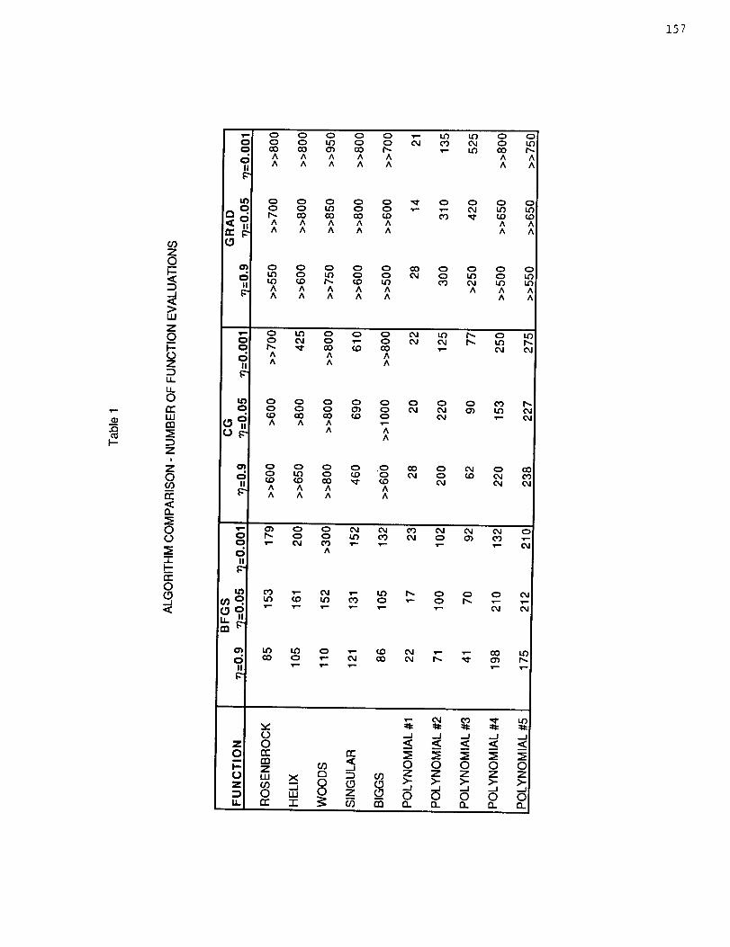
Results of Comparisons

Each of the test functions was optimized with a gradient (GRAD), conjugate

gradient (CG) and a Quasi-Newton technique (BFGS). Comparisons were made for

each test function and choice of algorithm based on the number of function

evaluations needed to approximate the true function minimum to within .0001.

Table i presents the measure of algorithm effectiveness for each of the ten

functions and for the nine algorithms that use Brent's one-dlmensional search

technique. Three possible search direction updates are considered, BFGS, CG,

and GRAD, and for each of those, three values for the gradient reduction

parameter, n = 0.9, 0.05, and 0.001, as the termination criterion for the

one-dlmenslonal searches.

157

9"

F-

O0

LU

Z

_o0Z

LL

L_o

LU

z,Zo

tT-

o0

I

00

[

I^^9-i <:3 0 <:3 0 O _- L_ li3 0

0 CO GO O_ 00 r'- _- li3 O0A A A A A A

O A A A A A A{{

o o o o o co o o o o• ;.o o Lo o o _ o LI3 o L,_

_0 I_ qD I.o co 04 I.oA A A A A A A_A A A A A A ^

v- o LO o o o o4 u3 r'_ o0

• A A A

{¢_ A A A

0 0 0 0 0 0 0 0 CO r-,

^ ,-.A

O_ 0 (:_ 0 0 .0 CO 0 0,I 0 O0• (:3 _ 0 _) 0 04 (:3 qD ¢xl

CO CO COA A A A

t_ A A A A

_- o_ o o oJ o4 co o4 ¢_ ¢_1 oo _-- o o _ co ol o o_ co _-

o ^|1

li_ 03 ,,'- i_; _" U9 l'_ 0 0 0 ¢xl

c_

II

158

For some of the table entries, numbers are preceded by either > or >>. In

both those cases, after 60 directional searches, the objective function was not

yet within .0001 of the minimum. If it were within .001 of the minimum, the

notation '>' is used with the nearest rounded-off number of total function

evaluations after the 60 searches. If the function remained greater than .001

away from the mln_mum after the 60 searches, the result in exactly the same

manner, the symbol '>>' was used to indicate that it is expected to take many

more evaluations to reach the stopping criterion.

The BFGS algorithm with _ = 0.9 clearly gives the best algorithm

performance, sometimes by an overwhelming amount when compared to gradient

methods. First, note that for eight of the ten test functions, BFGS with _ =

0.9 gives the best performance, and in the other two cases (Polynomials #I and

#4), it is not too far from the optimum. Second, note that for each of the

first five test functions, only one of the gradient algorithms requires fewer

than six times the number of function evaluations required by BFGS with n = 0.9

to achieve the desired measure of effectiveness. Even in that case (Singular

function), nearly four times as many evaluations are needed by the best

gradient technique to achieve the stated accuracy as are needed for the BFGS

algorithm with n = 0.9. Furthermore, in general, the BFGS algorithm with

n = 0.9 performs better than the BFGS algorithm with n = 0.05, which in turn

performs better than the BFGS algorithm with _ = 0.001.

These conclusions are quantified in several different ways. First, the

total number of function evaluations needed to reach the .0001 accuracy over

all ten functions for each algorithm are averaged. For the ten functions, the

BFGS, _ = 0.9 case averages 101.4 evaluations, the BFGS, n = 0.05 case averages

131.1 evaluations, and the BFGS, n = 0.001 case averages 152.2 evaluations,

with none of the gradient method algorithms averaging less than 380

evaluations. These sums are conservatively estimated for those methods with >

or >> as the table entries by assuming that in those cases, the number of

evaluations needed was * in the entry >>* or >*.

The first five test functions are the dominant effect in this disparity,

since none of the gradient methods perform adequately for any of these

functions. Since these five functions were constructed by researchers in the

field, they may represent function behavior that demonstrated the shortcomings

of a particular method and that occurred infrequently. With that in mind, the

same comparisons were performed for the five polynomial functions that were

159

constructed. The idea here was that a typical function that occurs in practice

lles somewhere "between" the first five test functions and the second five

functions, in terms of difficulty for the gradient methods to handle

efficiently.

For the five polynomials, the GRAD directional search technique still

performed poorly, especially for polynomials 4 and 5. For these polynomials,

the BFGS, _ = 0.9 case averages 101.4 evaluations, the BFGS, n " 0.05 case

averages 121.8 evaluations, and the BFGS, n - 0.001 case averages 111.4

evaluations, while the CG, n " 0.9 case averages 149.6 evaluations, the CG, _

0.05 case averages 142.0 evaluations, and the CG, n = 0.001 case averages 149.8

evaluations. Note that the BFGS, _ = 0.05 case had a higher average than the

BFGS, n _ 0.001 case for these polynomials was the result of the calculation

for polynomial #4. This is atypical, for among the ten test functions, the

BFGS, _ = 0.05 case gave superior performance to the BFGS, n - 0.001 case for

the first eight functions, with the last function giving virtually identical

performance for the two algorithms.

The BFGS, _ = 0.9 case is clearly the most efficient of the algorithms.

In turn, the BFGS, n _ 0.05 algorithm is the next most efficient, followed by

the BFGS, n = 0.001 case. The BFGS algorithms perform qualitatlvely better

than do the CG algorithms, which in turn perform qualitatively better than do

the GRAD algorithms. Stated differently, in all cases exhibited among the test

functions, the BFGS algorithms reached the .0001 approximation of the exact

minimum with reasonable efficiency. For some of those functions, both gradient

methods (CG and GRAD) were very inefficient (costly) in approximating the

minimum, while for another subset of the test functions, CG was reasonably

efficient at approximating the minimum while GRAD was not. It was never the

case that GRAD was efficient when CG was not, or that either gradient algorithm

was efficient when BFGS was not. The BFGS, _ = 0.9 case always worked with at

least a modest amount of improvement in efficiency over the alternative

methods, and sometimes the BFGS search methods gave dramatic reductions in the

number of evaluations needed to achieve the desired accuracy over the gradient

techniques. This method requires only function values at any point and

estimates approximate derivatives and Hessian matrices from function

evaluations.

160

PEPSIG OPTIMIZATIONS

In the current investigation, use of the PEPSIG analysis in conjunction

with formal optimization procedures to find optimum duct shapes is demonstrated

for realistic problems. The PEPSIG code is used to solve for the flow field in

the duct. The drop in mass average total (stagnation) pressure is used as the

performance index (objective function) for optimization. Each case was run

using approximately 200,000 grid points to provide the required accuracy. The

test case considered in this investigation involves optimizing a duct having an

offset bend for minimum pressure drop. The viscous flow calculations were

performed at a Reynolds number of 50,000 based on entrance mean velocity and at

a Math number of 0.3. The mass flow through the duct is held constant and the

pressure drop is non-dimensionalized with pu 2.

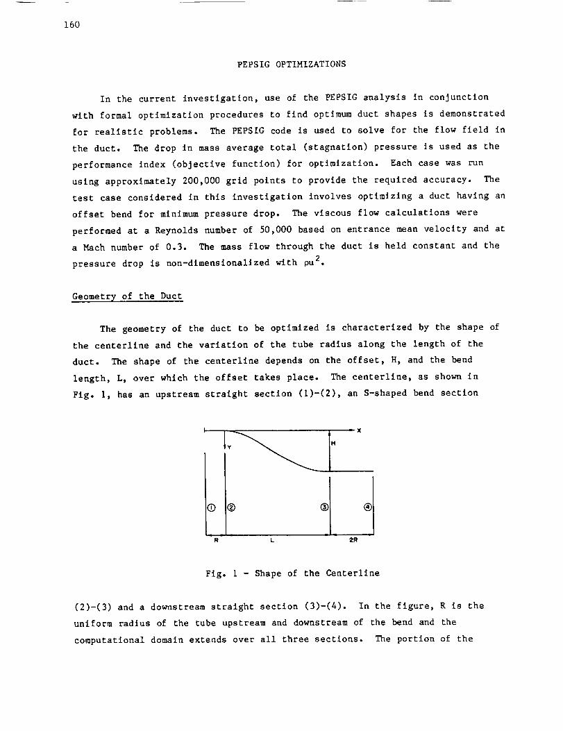
Geometry of the Duct

The geometry of the duct to be optimized is characterized by the shape of

the centerllne and the variation of the tube radius along the length of the

duct. The shape of the centerllne depends on the offset, H, and the bend

length, L, over which the offset takes place. The centerllne, as shown in

Fig. I, has an upstream straight section (I)-(2), an S-shaped bend section

s

I

R L

• X

Fig. 1 - Shape of the Centerllne

(2)-(3) and a downstream straight section (3)-(4). In the figure, R is the

uniform radius of the tube upstream and downstream of the bend and the

computational domain extends over all three sections. The portion of the

161

centerllne in the bend, i.e., section (2)-(3) is represented by a fifth order

polynomial with vanishing first and second derivatives at the end points and is

given as:

T[ = 10 - 15 + 6 (6)

One-parameter and two-parameter optimizations were performed in this study.

One-Parameter Optimizatlons:

A series of one-parameter optimlzations were performed to optimize

independently the parameters characterizing the duct geometry. First the bend

length, L, was optimized for a uniform duct of offset, H = I and radius, R = I.

If the bend length, L, is too large, there will be a large pressure drop due to

frictional losses. If the length is too small, there will be stronger

curvatures producing large pressure losses due to flow turning and separation.

Thus, there should exist an optimum bend length, L, that would strike a balance

between the two kinds of losses. This optimum value was found to be at

Lop t = 3.875 ± 0.015 and the corresponding pressure drop was A(PT) = 0.0336.

This will be used as a reference duct for comparison in the remaining

optimlzatlons.

It was seen for this optimum duct that there are significant regions of

flow separation due to the adverse pressure gradient resulting from the

curvature change about the inflexion point of the bend. If the separation

region is either suppressed or at least reduced to a smaller region, the losses

associated with separation may be reduced and an _mprovement in duct

performance may be obtained. One way to alleviate the adverse pressure

gradient is to contract the cross-sectional area of the duct in the region of

flow separation. A contraction will accelerate the flow, thus helping to

reduce separation. On the other hand, too much contraction may worsen the

performance because more reduction in area would mean higher velocities near

the minimum area, which would lead to higher friction losses. Also, since the

duct exit radius is held equal to the duct inlet radius, the divergence in the

duct following the contraction may lead to more flow separation. Thus, an

optimum contraction may exist and a one-parameter optimization was performed to

determine the optimum contraction for a fixed bend length, L.

162

I RI l R

-I 0 L! L t • L÷L!

2

R|I , X

L+2

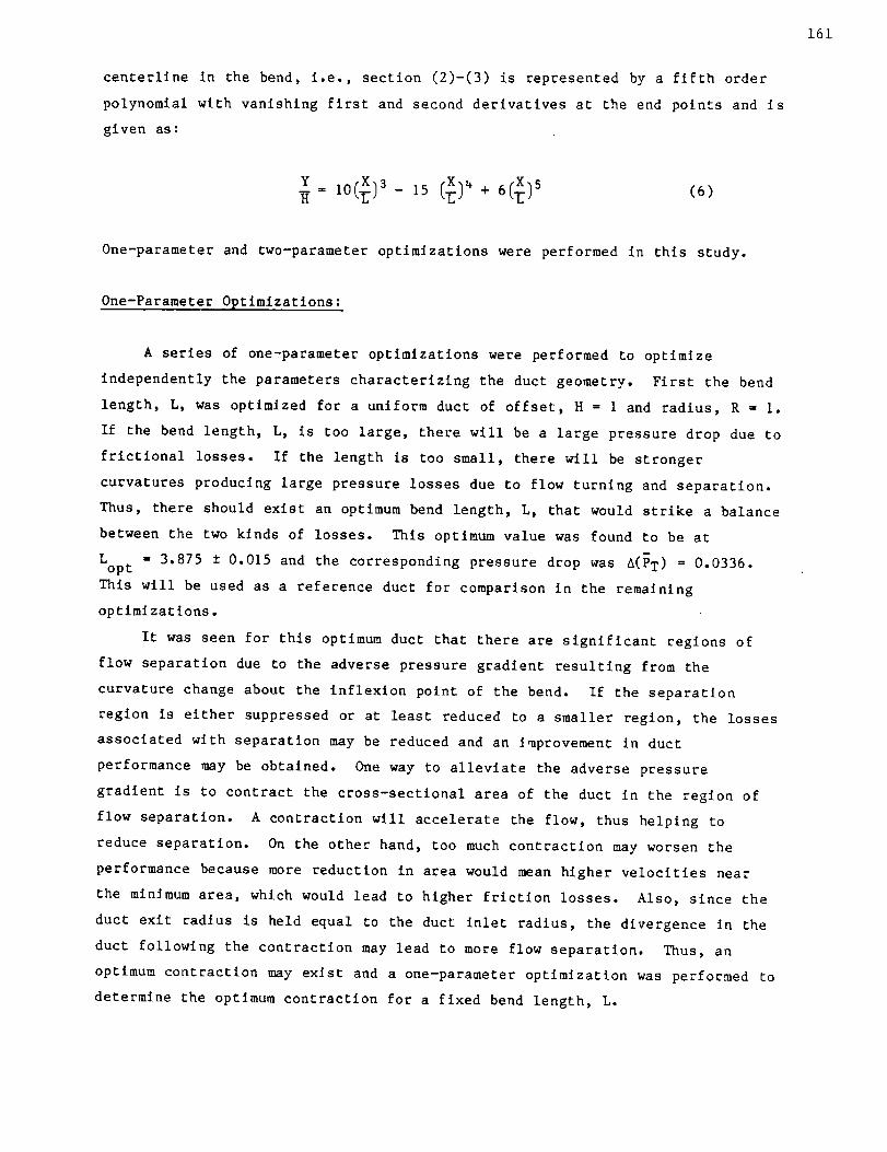
Fig. 2 - Variation of Duct Radius Along the Length of the Duct

The changing radius of the duct is shown in Fig. 2 and is represented by a

sixth order polynomial as follows. Rml n is the minimum radius of the duct.

-I <__X <__LI; R = R I (7)

L I <__X < L; R - A + BX + CX 2 + DX 3 + EX _ + FX 5 + GX 6 (8)

L_< X_< L + 2, R - R 2 (9)

The boundary conditions are:

dR d 2R

@ x - L_: R = Rt, dX d-_ 0 (10)

@ X = L 2 = L + L I ; R - Rmi n (II)2

dR d2R@ X = L: R = R2, --= - 0 (12)

dE

The seven coefficients A to G in Eq. (8) are evaluated using the boundary

conditions as given by Eqs. (I0) through (12). Fig. 3 shows the geometry of the

duct for this and subsequent optlmlzatlons. For L = 3.875, R I = R 2 = 1.0,

L 1 = 0.32L, L 2 - 0.66L and H = 1.0, Fig. 4 shows the variation of the pressure

drop with Rmi n and the optimum Rml n was found to be 0.97 ± 0.01 with a

pressure drop, A(P T) of 0.0322. For a reduction in the area of about 6%

corresponding to (Rmln)op t = 0.97, the pressure drop is reduced by about

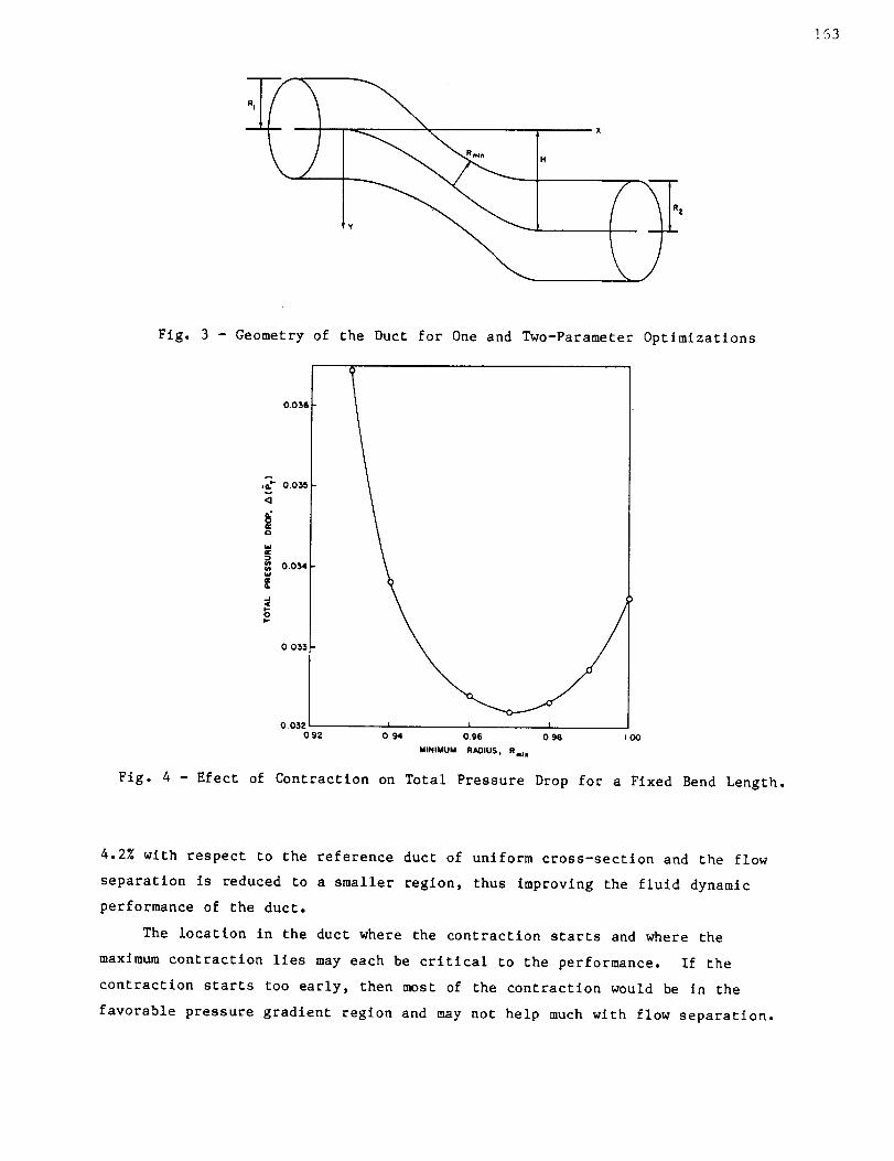
163

Fig. 3 - Geometry of the Duct for One and Two-Parameter Optlmlzatlons

0.036

,_ 0.0_

o

_ 0.0_

0.033

0032092

| A I0,94 096 0 96

MINIMUM RN)IUS, Rindn

OO

Fig. 4 - Efect of Contraction on Total Pressure Drop for a Fixed Bend Length.

4.2% with respect to the reference duct of uniform cross-section and the flow

separation is reduced to a smaller region, thus improving the fluid dynamic

performance of the duct.

The location in the duct where the contraction starts and where the

maximum contraction lles may each be critical to the performance. If the

contraction starts too early, then most of the contraction would be in the

favorable pressure gradient region and may not help much with flow separation.

164

If the contraction starts too far in the duct, it won't be effective in

improving the performance. In the next optimization, the location of the

start of the contraction, LI, is optimized for Rmi n = 0.97, L = 3.875 and

L + L I L + L 1L 2 = _ . (L 2 = ---./---- implies that contraction is symmetric about L 2 and

ends at the end of the bend.) Fig. 5 shows the effect of L I on the duct

performance and optimum L I was found to be 0.24L -+ 0.04 L with a pressure drop,

A(PT) , of 0.0320. This A(PT) is about 0.62% less than the A(P T) of the

previous optimization (corresponding to L 1 = 0.32L) and the overall reduction

in the pressure drop with respect to the reference case is about 4.8%.

0.0330

_ 0.0325 -

J

0.0_15

0.16

I I0.24 0.32 ).40

LOCATION OF THE START OF CONTRACTION, LI/L

Fig. 5 - Effect of Location of the Start of Contraction, LI,

on Total Pressure Drop.

Two-Parameter Optimlzatlons:

In the above one-parameter optlmlzations, the bend length, L, the

contraction, Rmln, and the start of the contraction, LI, were each optimized

independently for m_nimum pressure drop for a duct of fixed offset. However,

these parameters interact with each other and the optimization should be

performed in a way to account for this interaction. In the following examples,

two-parameter optlmlzations are performed where the two parameters are varied

simultaneously for an optimum combination. L and Rml n are the two parameters

to be optimized for a fixed L I. It was stated in the optimization section of

this report that the BFGS method is generally more efficient than the gradient

method for the examples considered. We will now demonstrate that the same is

true for realistic design problems such as a duct having an offset bend.

165

For a fixed offset, H = 1.0, R I = R 2 = 1.0, L I = 0.24L, L 2 = 0.62L,

optimum L and Rmi n are found using the gradient (steepest descent) and BFGS

methods. With the gradient method, three one-dimenslonal searchs were performed

and at the end of the third search the optimum values for L and Rmi n were

found to be 3.719 and 0.954, respectively. The pressure drop, A(P T) is

0.0305 and the cumulative number of function evaluations for thls method is

40. Using the BFGS method, two one-dlmenslonal searches were performed for a

comparable pressure drop as in the gradient method. The change in the search

direction is shown in Flg. 6. At the end of the second search using the BFGS

method, the pressure drop, A(PT) , Is 0.0306 and the cumulative number of

function evaluations Is seventeen. The optimum values for L and Rmi n are 3.559

and 0.958, respectively. Thus, for a comparable reduction in the pressure

drop, the BFGS method needed only approximately half the number of function

evaluations as that for the gradient method, reasserting that the BFGS method

is a more efficient method.

At the end of the second search of the BFGS optimization, the overall

reduction in the pressure drop compared to the reference case is about 9% and

the length of the duct was reduced by about 8%. The reduction in pressure loss

Is an improvement in duct performance. Decreases In length are usually

associated with reductions in weight and improved ease in packaging.

IO

0.9e

lJ

er096

ioI,-

_- 0,94z0(2

0.92

BF'GS ME'THO0

G_A01ENT METHO0

STARTING

POINT ]

O.9O, I I I I3.50 3.58 3.66 3.74 3.82 3.90

BEND LENGTH, L

Flg. 6 - Search Directions for BFGS and Gradient Methods of Optimization

166

CONCLUSIONS

Design of fluid dynamically efficient ducts is addressed through thecombination of optimization analysis with a three-dlmensional viscous fluid

dynamic analysis code. Since each function evaluation in the optimization

analysis is a three-dlmenslonal viscous flow analysis, which requires 200,000

grid points for accuracy, it is important to use both an efficient fluid

dynamic analysis and an efficient optimization technique. Three optimizationtechniques were evaluated on a series of test functions. The Quasi-Newton

(BFGS,n - .9) technique was selected as the prefected technique. A series of

basic duct design problems was performed. On a two-parameter optimization

problem the BFGStechnique was demonstrated to require half as manyfunctionevaluations as a steepest descent technique. Use of this parabolic flow

analysis rather than a full Navier-Stokes analysis in an optimization scheme

can provide huge computer run time and cost savings. Optimization of realistic

aerodynamic and hydrodynamic ducts can nowbe madea routine part of the design

process for approximately the computer time required for a single functionevaluation using an efficient three-dimenslonal Navier-Stokes analysis.

ACKNOWLEDGEMENT

This work was sponsored by NASALewis Research Center, Cleveland, Ohio.

REFERENCES

IQ Levy, R., Briley, W.R. and McDonald, H.: Viscous Prlmary/Secondary Flow

Analysis for Use with Non-Orthogonal Coordinate Systems, AIAA Paper

83-0556, 1983.

. Towne, C.E.: Computation of Viscous Flow in Curved Ducts and Comparison

with Experimental Data, AIAA Paper 84-0531, 1984.

. Scales, L.E.: Introduction to Non-Linear Optimization. Springer-Verlag,

New York, 1985.

. Gill, P.E., Murray, W. and Wright, M.H.: Practical Optimization.

Academic Press, London, 1981.