nanostructured fluorinated molecular films · hidrogenado, foi possível estimar um diagrama de...

Nanostructured fluorinated molecular films

Ana Carolina Monteiro Pedrosa

Thesis to obtain the Master of Science Degree in

Integrated Master in Chemical Engineering

Supervisors: Prof. Dr. Eduardo Filipe (IST)

Prof. Dr. Michel Goldmann (INSP)

Examination Committee

Chairperson (Presidente): Prof. Dr. António Maçanita

Supervisor (Orientador): Prof.Dr. Eduardo Filipe

Member of the Committee (Vogal): Prof. Dra. Isabel Marrucho

16 November 2017

III

“La glorie se donne seulement à ceux

qui l'ont toujours rêvée.“

Charles de Gaulle

V

Acknowledgements

The realization of this master thesis would not be possible without the collaboration of people

who were essential for the evolution and conclusion of this project. Firstly, I would like to thank Professor

Eduardo Filipe for presenting me this theme and opportunity that I was very glad to accept. Secondly,

to the INSP for accepting me with open arms and helping me feel comfortable and well welcomed. To

Professor Michel Goldmann a big thank for all the guidance, support and dedication in helping me with

this project. I would also like to thank Professor Marie-Claude Fauré for assisting me in the realization

of the experimental techniques and interpretation of the results and to Richard Soucek for helping me

with the synthesis of the semi-fluorinated compound and other laboratory works. Thirdly, I thank the

SOLEIL Synchrotron and specially Dr. Philippe Fontaine for assisting in the realization of the X-Ray

diffraction experiments.

VII

Abstract

In the present work, it is proposed to better understand the behaviour of hydrogenated and

fluorinated mixtures. By studying mixtures with various concentrations, from high fluorinated to high

hydrogenated percentage, it is possible to estimate a phase diagram. This phase diagram is crucial for

further understanding the phase changes according to variations of pressure and concentration. The

compounds studied in these mixtures were the Myristic Acid (C13H27COOH) and the

Perfluorododecanoic Acid (C11F23COOH), through Langmuir film, Brewster Angle Microscopy and

Grazing Incidence X-Ray diffraction techniques. It was verified that the diffraction peak of the fluorinated

compound is 12,5nm-1 while the hydrogenated is 15nm-1.

Following the same Langmuir film and Grazing Incidence X-Ray diffraction techniques,

fluorinated alcohols such as F14OH (F(CF2)13CH2OH) and F18OH (F(CF2)17CH2OH) were studied. Both

compounds present a diffraction peak around 12,6nm-1 which suggests the existence of a crystalline

structure. However, for some values of pressure, the F18OH has a double peak that might indicate a

different configuration or the existence of tilted molecules. A mixture of F18OH and Perfluorododecanoic

Acid was analysed and the X-Ray diffraction results confirmed the existence of complete segregation

between both compounds.

As an exploratory work, the semi fluorinated alkane F8H14 (F(CF2)8(CH2)14H) was studied under

Langmuir film and Grazing Incidence X-Ray diffraction techniques. By analysing its behaviour through

the isotherms, it is possible to verify the collapse of the monolayer and further stabilization of the film

until it collapses at a possible double-layer or tri-layer structure.

Keywords

Langmuir films

Isotherm

Brewster Angle Microscopy

X-Ray Diffraction

Semi-fluorinated alkanes

Fluorinated alcohols

IX

Resumo

No presente trabalho, propõe-se obter uma melhor compreensão do comportamento das

misturas de compostos fluorados e hidrogenados. Ao estudar misturas com variadas concentrações,

desde percentagens elevadas de composto fluorado a percentagens elevadas de composto

hidrogenado, foi possível estimar um diagrama de fase. Este diagrama de fase é crucial para o melhor

entendimento das mudanças de fase de acordo com variações de pressão e concentração. Os

compostos estudados nestas misturas foram o Ácido Mirístico (C13H27COOH) e o Ácido

Perfluorododecanóico (C11F23COOH), através de filmes de Langmuir, Microscopia de Ângulo de

Brewster e Difração de Raios X. Foi verificado que o pico de difração para o composto fluorado era

cerca de 12,5nm-1 enquanto que para o composto hidrogenado este valor foi de 15nm-1.

Seguindo as mesmas técnicas de filmes de Langmuir e Difração de Raios X, álcoois fluorados

como o F14OH (F(CF2)13CH2OH) e o F18OH (F(CF2)17CH2OH) foram estudados. Ambos os compostos

apresentaram um pico de difração a cerca de 12,6nm-1, o que sugere a existência de estrutura cristalina.

Contudo, para alguns valores de pressão, o F18OH apresenta duplo pico de difração o que pode indicar

uma diferente configuração ou a existência de moléculas inclinadas. Ao analisar uma mistura de F18OH

e Ácido Perfluorododecanóico através da Difração de Raios X, foi possível confirmar a existência de

segregação total entre os dois compostos.

Como trabalho exploratório, o alcano semi fluorado F8H14 (F(CF2)8(CH2)14H) foi estudado

através de filmes de Langmuir e Difração de Raio X. Ao analisar o comportamento das isotérmicas foi

possível verificar o colapso da monocamada seguido de uma estabilização do filme até colapsar numa

possível estrutura de duas ou três camadas.

Palavras-Chave

Filmes de Langmuir

Isotérmica

Microscopia de Ângulo de Brewster

Diffração de Raios X

Alcanos semifluorados

Álcoois fluorados

XI

Acronyms

a.u. – Arbitrary Unit

BAM – Brewster Angle Microscopy

GIXD – Grazing Incidence X-Ray Diffraction

GISAXS – Grazing Incidence Small Angle X-Ray Scattering

LC – Liquid Condensed

LE – Liquid Expanded

P - Pressure

T* - Critical Temperature

T0 – triple Point Temperature

xc – Position of the peak for the X-Ray diffraction results

w – Width of the peak for the X-Ray diffraction results

2D – two dimensional

3D – three dimensional

XIII

Table of Contents

Acknowledgements ................................................................................................................................. V

Abstract.................................................................................................................................................. VII

Keywords ............................................................................................................................................... VII

Resumo .................................................................................................................................................. IX

Palavras-Chave ...................................................................................................................................... IX

Acronyms ................................................................................................................................................ XI

Index to Tables .....................................................................................................................................XVI

Index to Figures ....................................................................................................................................XVI

I. Introduction ...................................................................................................................................... 1

I.1 Motivation/Purpose ..................................................................................................................... 1

I.2 Semi-fluorinated n-alkanes ......................................................................................................... 1

I.3 Fluorinated Alcohols ................................................................................................................... 2

I.4 Surface Tension and Surface Pressure ...................................................................................... 3

I.5 Compressibility ........................................................................................................................... 4

I.6 Surface Crystallography ............................................................................................................. 4

I.7 Experimental Method .................................................................................................................. 7

I.7.1 Langmuir Film, Langmuir Trough ........................................................................................ 7

I.7.2 Brewster Angle Microscopy ................................................................................................ 9

I.7.3 Grazing Incidence X-Ray Diffraction and Synchrotron Radiation ..................................... 10

II. Results and Discussion ................................................................................................................. 13

II.1 Chemical Compounds and solvents ......................................................................................... 13

II.2 H13COOH ................................................................................................................................ 15

II.2.1 Isotherms .......................................................................................................................... 15

II.2.2 BAM images ...................................................................................................................... 17

II.2.3 X-Ray Diffraction ............................................................................................................... 18

II.3 Fluorinated Compounds ........................................................................................................... 19

II.3.1 F11COOH ......................................................................................................................... 19

II.3.1.1 Isotherms ................................................................................................................... 19

XIV

II.3.1.2 BAM images .............................................................................................................. 21

II.3.1.3 X-Ray Diffraction........................................................................................................ 22

II.3.2 F14OH ............................................................................................................................... 26

II.3.2.1 Isotherms ................................................................................................................... 26


II.3.3 F18OH ............................................................................................................................... 30

II.3.3.1 Isotherms ................................................................................................................... 30


II.4 Mixture ...................................................................................................................................... 35

II.4.1 F11COOH and F18OH ..................................................................................................... 35

II.4.2 F11COOH and H13COOH ................................................................................................ 37

II.4.2.1 Isotherms ................................................................................................................... 37

II.4.2.2 BAM images .............................................................................................................. 41

20% F11COOH & 80% H13COOH ...................................................................... 41

70% F11COOH & 30% H13COOH ...................................................................... 44


20% F11COOH & 80% H13COOH ...................................................................... 45

35% F11COOH & 65% H13COOH ...................................................................... 50

60% F11COOH & 40% H13COOH ...................................................................... 53

70% F11COOH & 30% H13COOH ...................................................................... 55

II.4.2.4 Phase Diagram .......................................................................................................... 58

II.5 F8H14 ....................................................................................................................................... 64

II.5.1 Isotherms .......................................................................................................................... 64

II.5.2 X-Ray Diffraction ............................................................................................................... 65

III. Conclusions and Future Work ....................................................................................................... 67

IV. References ..................................................................................................................................... 69

V. Appendix .......................................................................................................................................... 1

V.1 Stability Tests ............................................................................................................................. 1

V.2 X-Ray Diffraction ......................................................................................................................... 3

V.2.1 H13COOH ........................................................................................................................... 3

XV

V.2.2 F11COOH ........................................................................................................................... 3

V.2.3 F14OH ................................................................................................................................. 5

V.2.4 F18OH ................................................................................................................................. 6

V.2.5 F11COOH and F18OH ....................................................................................................... 7

V.2.6 F11COOH and H13COOH .................................................................................................. 8

VI. Notes .............................................................................................................................................. 10

XVI

Index to Tables

Table 1 - The five two-dimensional nets and their characteristics. ......................................................... 4

Table 2 - Properties of the chemical compounds used in the experiment. ........................................... 13

Table 3 - Concentrations of the F11COOH + H13COOH solutions. ..................................................... 13

Table 4 - Solvents used in the experiment. ........................................................................................... 14

Table 5 - Ratio between F11COOH peak positions at 6°C for different values of pressure. ................ 24

Table 6 - Ratio between F14OH peak positions at 22°C for different values of pressure. ................... 28

Table 7 - Ratio between F18OH peak positions at 18°C for different values of pressure. ................... 32

Table 8 - X-Ray diffraction peaks for F18OH at 18°C and 10mN/m. .................................................... 33

Table 9 - Compressibility values for the five mixtures and pure compounds at 22°C and 6°C with the

correspondent regions between which the compressibility was calculated. ......................................... 39

Table 10 - Acronyms used to simplify the understanding of the phase diagram. ................................. 58

Table 11 - Compressibility values of the F8H14 at 20°C, 18°C, 15°C and 5°C and the correspondent

region between which the compressibility was calculated. ................................................................... 65

Index to Figures

Figure 1 - Molecular model of semi-fluorinated alkanes. ........................................................................ 1

Figure 2 - Semi-fluorinated alkanes in air/water interface, their domains and formations. ..................... 2

Figure 3 - Representation of the F18OH, on the left, and F14OH, on the right, used in this work. ........ 2

Figure 4 – Microscopic view of a liquid droplet and its cohesive forces of a molecule at the surface and

in the bulk. ............................................................................................................................................... 3

Figure 5 - Five two-dimensional Bravais lattices where a and b represent the lengths of unit-mesh

edges and ɣ characterises the interaxial angle. ...................................................................................... 5

Figure 6 – Representation of a real Bravais lattice, on the left, and a reciprocal lattice, on the right. .... 5

Figure 7 - Relationship between real space basic vectors a and b and reciprocal space basic vectors

a* and b*. ................................................................................................................................................. 6

Figure 8 - Reciprocal lattice points for a two-dimensional layer where the bar over the number, such as

1, represent s a negative number. ........................................................................................................... 6

Figure 9 - Representation of a section of a two-dimensional reciprocal lattice and the (1 1) and (2 0)

peaks. ...................................................................................................................................................... 7

XVII

Figure 10 – Representation of a standard Langmuir trough where: 1 - Frame, 2- Surface Pressure

sensor, 3- Barriers, 4- Trough top. .......................................................................................................... 8

Figure 11 – Schematic diagram of a Langmuir trough (top) and a generalized isotherm of a Langmuir

monolayer where the surface pressure is represented with respect to the area per molecule. .............. 8

Figure 12 - The principle of Brewster Angle Microscopy. ........................................................................ 9

Figure 13 - Simplified BAM scheme. ....................................................................................................... 9

Figure 14 - Schematic of the Symmetric GIXD geometry. .................................................................... 10

Figure 15 – SOLEIL Synchrotron structural scheme. ............................................................................ 11

Figure 16 - Adjustment of a peak from X-Ray diffraction experiments, using the Lorentz model in

Origin program. ...................................................................................................................................... 11

Figure 17 - Isotherms of pure H13COOH at low temperatures and the disappearance of the LE phase

at 6°C. .................................................................................................................................................... 15

Figure 18 - Isotherms of pure H13COOH at 6°C and 22°C. ................................................................. 15

Figure 19 - BAM images for pure H13COOH at 22°C. .......................................................................... 17

Figure 20 - Position of the diffraction peak of pure H13COOH with respect to the pressure at 6°C. ... 18

Figure 21 - X-Ray diffraction result for the pure H13COOH at 22°C. ................................................... 18

Figure 22 - Isotherms of pure F11COOH at 6°C and 22°C. .................................................................. 19

Figure 23 - Molecular orientation at the air/water interface as a function of barrier positions. ............. 19

Figure 24 - BAM images for pure F11COOH at 22°C. .......................................................................... 21

Figure 25 - Diffraction spectra for the pure F11COOH at 18°C for different pressures, represented by

the logarithm of intensity with respect to the peak position. .................................................................. 22

Figure 26 - Position of the (10) peak of F11COOH with respect to the pressure at 18°C. ................... 22

Figure 27 - Diffraction spectra for the pure F11COOH at 6°C for different pressures, represented by

the logarithm of intensity with respect to the peak position. .................................................................. 23

Figure 28 - Position of the (10) peak of F11COOH with respect to the pressure at 6°C. ..................... 23

Figure 29 - Ratio between F11COOH peak positions at 6°C with respect to the pressure. ................. 24

Figure 30 - Logarithm of area per molecule of F11COOH with respect to the pressure at 18°C. ........ 25

Figure 31 - Logarithm of area per molecule of F11COOH with respect to the pressure at 6°C. .......... 25

Figure 32 - Isotherms of F14OH at 14°C and 22°C .............................................................................. 26

Figure 33 - Diffraction spectra for the pure F14OH at 22°C for different pressures, represented by the

logarithm of intensity with respect to the peak position. ........................................................................ 27

Figure 34 – Position of the (10) peak of F14OH with respect to the pressure at 22°C. ........................ 27

XVIII

Figure 35 - Ratio between F14OH peak positions with respect to the pressure. .................................. 28

Figure 36 - Logarithm of area per molecule of F14OH with respect to the pressure at 22°C. .............. 29

Figure 37 - Intensity with respect to the area per molecule for the plateau of the isotherm at 22°C. ... 29

Figure 38 - Beginning of the plateau obtained experimentally for F14OH at 22°C. .............................. 30

Figure 39 - Isotherms of F18OH at 14°C and 22°C. ............................................................................. 30

Figure 40 - Diffraction spectra for the pure F18OH at 18°C for different pressures, represented by the

logarithm of intensity with respect to the peak position. ........................................................................ 31

Figure 41 – Position of the (10) peak of F18OH with respect to the pressure at 18°C. ........................ 32

Figure 42 - Ratio between F18OH peak positions with respect to the pressure. .................................. 33

Figure 43 - Relation between the "a" and "b" network parameters. ...................................................... 34

Figure 44 - Logarithm of area per molecule of F18OH with respect to the pressure at 18°C. .............. 34

Figure 45 - Diffraction spectra for the F11COOH + F18OH mixture at 18°C for different pressures,

represented by the logarithm of intensity with respect to the peak position. ......................................... 35

Figure 46 – Position of the (10) peak of F11COOH and F18OH co-deposition with respect to the

pressure at 18°C. ................................................................................................................................... 36

Figure 47 - Isotherms of pure H13COOH, pure F11COOH and three different concentrations (%vol)

created by co-depositing different volumes of each pure compound on the trough at 18°C. ............... 37

Figure 48 - Isotherms for the five different mixtures of F11COOH + H13COOH at 22°C and the

previously recorded isotherms of the pure fluorinated and hydrogenated compounds. ....................... 38

Figure 49 - Isotherms for the five different mixtures of F11COOH + H13COOH at 6°C and the

previously recorded isotherms of the pure fluorinated and hydrogenated compounds. ....................... 38

Figure 50 - Example of a perfect hexagonal structure, on the left, formed by hydrogenated molecules

followed by a non-perfect hexagonal structure, on the right, formed by hydrogenated molecules and

one fluorinated molecule, with a higher atomic radius. ......................................................................... 39

Figure 51 - Relation between the compressibility values calculated from the isotherms at 22°C and the

percentage of F11COOH on the mixtures. ............................................................................................ 40

Figure 52 - Relation between the compressibility values calculated from the isotherms at 6°C and the

percentage of F11COOH on the mixtures. ............................................................................................ 40

Figure 53 - BAM images for the 20%F11COOH & 80%H13COOH mixture at 22°C. ........................... 41


Figure 55 - BAM images for the 20%F11COOH & 80%H13COOH mixture at 6°C. ............................. 43


Figure 57 - BAM images for the 70%F11COOH & 30%H13COOH mixture at 6°C. ............................. 45

XIX

Figure 58 - Diffraction spectra for the 20%F11COOH & 80%H13COOH mixture at 22°C for different

pressures, represented by the logarithm of intensity with respect to the peak position. ....................... 46

Figure 59 - Position of the peak of 20%F11COOH & 80%H13COOH mixture with respect to the

pressure at 22°C. ................................................................................................................................... 46

Figure 60 - Width of the peak of 20%F11COOH & 80%H13COOH mixture with respect to the pressure

at 22°C. .................................................................................................................................................. 46




pressure at 14°C where the blue dots represent the fluorinated type molecules and the orange dots

the hydrogenated. .................................................................................................................................. 48


at 14°C where the blue dots represent the fluorinated type molecules and the orange dots the

hydrogenated. ........................................................................................................................................ 48




pressure at 6°C where the blue dots represent the fluorinated type molecules and the orange dots the

hydrogenated. ........................................................................................................................................ 49



hydrogenated. ........................................................................................................................................ 49





the hydrogenated. .................................................................................................................................. 50



hydrogenated. ........................................................................................................................................ 50



Figure 71 - Representation of the moment of the collapse for the 35%F11COOH & 65%H13COOH at

45mN/m. ................................................................................................................................................ 52

XX



hydrogenated. ........................................................................................................................................ 52



hydrogenated. ........................................................................................................................................ 52




pressure at 22°C where the blue dots represent the fluorinated type molecules and the orange dot the

hydrogenated. ........................................................................................................................................ 53


at 22°C where the blue dots represent the fluorinated type molecules and the orange dot the

hydrogenated. ........................................................................................................................................ 53

Figure 77 - Representation of a regular X-Ray diffraction signal, on the left, and the moment of the

collapse, on the right, which is represented by a single point at different position. .............................. 54





hydrogenated. ........................................................................................................................................ 55



hydrogenated. ........................................................................................................................................ 55



Figure 82 - Representation of the moment of the collapse for the 70%F11COOH & 30%H13COOH at

45mN/m. ................................................................................................................................................ 56



hydrogenated. ........................................................................................................................................ 57



hydrogenated. ........................................................................................................................................ 57



XXI



hydrogenated. ........................................................................................................................................ 58



hydrogenated. ........................................................................................................................................ 58

Figure 88 – Results obtained from the X-Ray diffraction experiments plotted on the phase diagram of

the Fluorinated and Hydrogenated mixtures at 22°C where the red lines represent the change of

phase. .................................................................................................................................................... 59

Figure 89 - Phase diagram of the fluorinated and hydrogenated mixture at 22°C where the dashed

lines represent uncertain limits. ............................................................................................................. 60

Figure 90 - Phase diagram of the fluorinated and hydrogenated mixture at 22°C with the inclusion of a

broader gas phase, where the dashed lines represent uncertain limits. ............................................... 61

Figure 91 - Phase diagram of the fluorinated and hydrogenated mixture at 6°C where the dashed line

represents an uncertain limit. ................................................................................................................ 62

Figure 92 - Phase diagram of the fluorinated and hydrogenated mixture at 6°C with the inclusion of a

broader gas phase, where the dashed lines represent uncertain limits. ............................................... 63

Figure 93 - Isotherms of F8H14 at 5°C, 15°C, 18°C and 20°C. ............................................................ 64

Figure 94 - Position of the peak of F8H14 with respect to the pressure at 18°C. ................................. 65

Figure 95 - Width of the peak of F8H14 with respect to the pressure at 18°C...................................... 65

Figure A 1 - Stability test for the 60%F11COOH & 40%H13COOH at 6°C with a resting time of 30

minutes. ................................................................................................................................................... 1

Figure A 2 - Stability test for the F8H14 at 15°C with a resting time of 15 minutes. ............................... 1



Figure A 5 - Width of the diffraction peak of pure H13COOH with respect to the pressure at 6°C......... 3

Figure A 6 - Area of the diffraction peak of pure H13COOH with respect to the pressure at 6°C. ......... 3

Figure A 7 - Width of the (10) diffraction peak of pure F11COOH with respect to the pressure at 6°C. 3

Figure A 8 - Area of the (10) diffraction peak of pure F11COOH with respect to the pressure at 6°C. .. 3

Figure A 9 - Position of the (11) diffraction peak of pure F11COOH with respect to the pressure at 6°C.

................................................................................................................................................................. 3

XXII

Figure A 10 - Position of the (20) diffraction peak of pure F11COOH with respect to the pressure at

6°C. .......................................................................................................................................................... 3

Figure A 11 - Width of the (11) diffraction peak of pure F11COOH with respect to the pressure at 6°C.

................................................................................................................................................................. 4


................................................................................................................................................................. 4

Figure A 13 - Area of the (11) diffraction peak of pure F11COOH with respect to the pressure at 6°C. 4

Figure A 14 - Area of the (20) diffraction peak of pure F11COOH with respect to the pressure at 6°C. 4

Figure A 15 - Width of the (10) diffraction peak of pure F11COOH with respect to the pressure at

18°C. ........................................................................................................................................................ 4

Figure A 16 - Area of the (10) diffraction peak of pure F11COOH with respect to the pressure at 18°C.

................................................................................................................................................................. 4

Figure A 17 - Width of the (10) diffraction peak of F14OH with respect to the pressure at 22°C. .......... 5

Figure A 18 - Area of the (10) diffraction peak of F14OH with respect to the pressure at 22°C. ............ 5

Figure A 19 - Position of the (11) diffraction peak of F14OH with respect to the pressure at 22°C........ 5






Figure A 25 - Width of the (10) diffraction peak of F18OH with respect to the pressure at 18°C, where

the orange triangles represent the sum of the values of the double peak. ............................................. 6

Figure A 26 - Area of the (10) diffraction peak of F18OH with respect to the pressure at 18°C, where

the orange triangles represent the sum of the values of the double peak. ............................................. 6







Figure A 33 - Width of the (10) peak of F11COOH and F18OH co-deposition with respect to the

pressure at 18°C. ..................................................................................................................................... 7

XXIII

Figure A 34 - Area of the (10) peak of F11COOH and F18OH co-deposition with respect to the

pressure at 18°C. ..................................................................................................................................... 7

Figure A 35 - Area of the peak of 20%F11COOH & 80%H13COOH mixture with respect to the


hydrogenated. .......................................................................................................................................... 8



the hydrogenated. .................................................................................................................................... 8


pressure at 22°C. ..................................................................................................................................... 8



hydrogenated. .......................................................................................................................................... 9



the hydrogenated. .................................................................................................................................... 9



hydrogenated. .......................................................................................................................................... 9



hydrogenated. .......................................................................................................................................... 9



hydrogenated. .......................................................................................................................................... 9



hydrogenated ........................................................................................................................................... 9

1

I. Introduction

I.1 Motivation/Purpose

The semi-fluorinated compounds can be used in medicine as they are biologically stable and

able to improve the stability and permeability of liposomes (Sabín, Prieto, Estelrich, Sarmiento & Costas,

2010). As the perfluorinated block segregates with H atoms, the study of semi-fluorinated molecules is

crucial as it is necessary that the hydrogenated chain is inside the cell and the fluorinated chain is

outside dissolving oxygen and working as blood substitute in surgeries.

The main purpose of this study is to understand the behaviour and characteristics of semi-

fluorinated molecules and fluorinated alcohols as well as the mixtures of fluorinated and hydrogenated

species at the interface. Ultimately, the aim is to comprehend and control the formation of domains and

patterns.

I.2 Semi-fluorinated n-alkanes

Semi-fluorinated alkanes, also known as FnHm, are formed by a fluorinated chain linked to a

hydrogenated chain which allows them to have the unique feature of being both strongly hydrophobic

and lipophobic (Sabín, Prieto, Estelrich, Sarmiento & Costas, 2010). Despite the absence of hydrophilic

group, the simultaneous presence of lipophobic and hydrophobic segments gives these molecules the

ability to form various supramolecular nano-structures, which can be used for numerous applications

from medicine to smart-materials and tailored interfaces (Fontaine, P., Bardin, L. Faure, M.-C., Filipe,

E. & Goldmann, M., 2017).

Figure 1 - Molecular model of semi-fluorinated alkanes.

The fluorinated chain is bulkier than the hydrogenated chain as their atomic radius is higher than

the hydrogen atoms, as represented on figure 1. Both fluorocarbon and hydrocarbon chains are non-

polar and have a cylindrical structure.

Since the pioneering work that demonstrated semi-fluorinated alkanes form Langmuir

monolayers at the air/water interface, (Gaines, G.L, 1991) their structure has remained controversial.

These monolayers have been the subject of many studies using different preparation and

characterization techniques.

Using GISAXS it is possible to prove that these water insoluble molecules form highly organized

domains with hexagonal structure (Bardin, L., Faure, M.C, Filipe, E., Fontaine, P. & Goldmann, M.,

Fluorinated chain

Hydrogenated chain

2

2010). The FnHm monolayers segregate vertically, spontaneously or upon compression, when mixed

with other compounds such as phospholipids, polymers, copolymers or peptides. Their segregation into

larger domains is represented on figure 2. Thermodynamical studies have shown that, when stable at

water surface, FnHm monolayers have a surface density of about 0,3 nm2/molecule, which is similar to

the fluorinated chain’s value. This suggests that the packing of the molecule is mainly determined by

the fluorinated chain (Bardin, L., Faure, Limagne, D., Chevallard, C. et al, 2011).

Figure 2 - Semi-fluorinated alkanes in air/water interface, their domains and formations. (Vlassopoulos, D., Geue, T., Müllen, et al, 2013)

I.3 Fluorinated Alcohols

The polyfluorinated alcohols are a class of compounds recently identified as precursor

molecules to the perfluorinated acids detected on the environment. These compounds are used in

synthesis of various fluorosurfactants and incorporated in polymeric materials used extensively in the

carpet, textile and paper industries (Dinglasan-Panlilio, M.J.A, Mabury, S.A, 2006).

Long chain alcohols such as 1H,1H-Perfluoro-1-Tetradecanol (F14OH) and 1H,1H-Perfluoro-1-

Octadecanol (F18OH) are insoluble in water which allows them to form Langmuir films at the surface of

water (Teixeira, M. 2014). These alcohols are represented on figure 3, with F18OH on the left and

F14OH on the right. The alcohol head group guarantees the adequate orientation at the air/water

interface and anchoring of the molecules at the interface.

Figure 3 - Representation of the F18OH, on the left, and F14OH, on the right, used in this work. (Teixeira, M. 2014)

3

I.4 Surface Tension and Surface Pressure

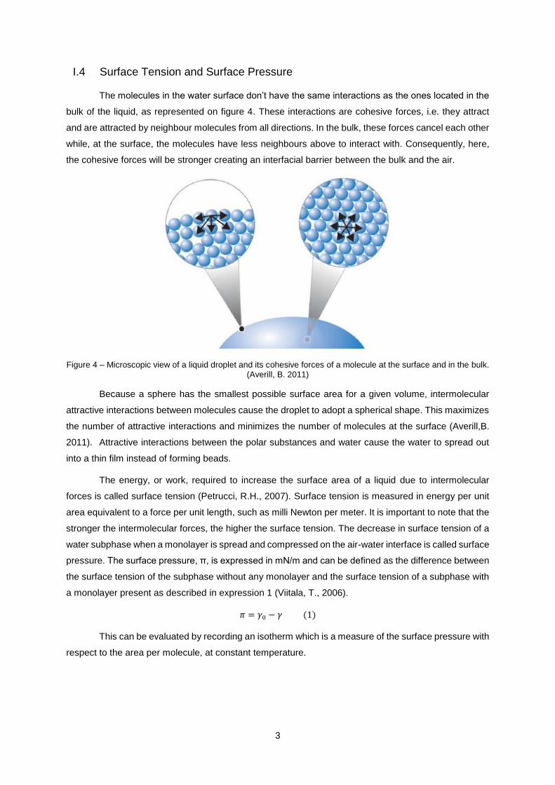
The molecules in the water surface don’t have the same interactions as the ones located in the

bulk of the liquid, as represented on figure 4. These interactions are cohesive forces, i.e. they attract

and are attracted by neighbour molecules from all directions. In the bulk, these forces cancel each other

while, at the surface, the molecules have less neighbours above to interact with. Consequently, here,

the cohesive forces will be stronger creating an interfacial barrier between the bulk and the air.

Figure 4 – Microscopic view of a liquid droplet and its cohesive forces of a molecule at the surface and in the bulk. (Averill, B. 2011)

Because a sphere has the smallest possible surface area for a given volume, intermolecular

attractive interactions between molecules cause the droplet to adopt a spherical shape. This maximizes

the number of attractive interactions and minimizes the number of molecules at the surface (Averill,B.

2011). Attractive interactions between the polar substances and water cause the water to spread out

into a thin film instead of forming beads.

The energy, or work, required to increase the surface area of a liquid due to intermolecular

forces is called surface tension (Petrucci, R.H., 2007). Surface tension is measured in energy per unit

area equivalent to a force per unit length, such as milli Newton per meter. It is important to note that the

stronger the intermolecular forces, the higher the surface tension. The decrease in surface tension of a

water subphase when a monolayer is spread and compressed on the air-water interface is called surface

pressure. The surface pressure, π, is expressed in mN/m and can be defined as the difference between

the surface tension of the subphase without any monolayer and the surface tension of a subphase with

a monolayer present as described in expression 1 (Viitala, T., 2006).

𝜋 = 𝛾0 − 𝛾 (1)

This can be evaluated by recording an isotherm which is a measure of the surface pressure with

respect to the area per molecule, at constant temperature.

4

I.5 Compressibility

The coefficient of compressibility is a measure of the relative surface change of fluid or solid as

a response to a pressure change. For any system, the magnitude of the compressibility depends

strongly on whether the process is adiabatic or isothermal (Fine, R. A., 1973). Therefore, isothermal

compressibility was considered since all the isotherms are recorded at constant temperature. The

compressibility is measured in m/N and can be described by expression 2.

𝜒 = −1

𝐴(

𝑑𝐴

𝑑𝑃)

𝑇 (2)

Where A is the mean molecular area which is calculated automatically by the Langmuir trough

according to the amount of solution added into the subphase and P is the corresponding surface

pressure (Bhande, R. S., 2012).

I.6 Surface Crystallography

Any solid material in which the component atoms are arranged in a definite pattern and whose

surface regularity reflects its internal symmetry is considered a crystal.

The unit cell is the smallest unit in volume that permits identical cells to be stacked together to

fill a space. By repeating the pattern of the unit cell over and over in all directions, the entire crystal

lattice, i.e. the crystal structure, can be constructed. An important characteristic of a unit cell is the

number of atoms it contains. The total number of atoms in the entire crystal is the number in each cell

multiplied by the number of unit cells (Mahan, G. D., 2016).

In triperiodic structures the equivalent points form a three-dimensional lattice in which the space

units are unit cells. In diperiodic structures the equivalent points for a two-dimensional new in which the

area units are unit meshes (Wood, E. A., 1964). The 14 Bravais space lattices are replaced, in the

diperiodic case, by 5 nets as described on table 1 and figure 5, where the ≠ symbol implies nonequality

by reason of symmetry even though accidental equality may occur, a and b represent the lengths of

unit-mesh edges and ɣ characterises the interaxial angle.

Table 1 - The five two-dimensional nets and their characteristics.

Shape of unit mesh Nature of axes Nature of angles Name of corresponding system

General parallelogram a ≠ b ɣ ≠ 90° Oblique

Rectangle a ≠ b ɣ = 90° Rectangular

Centered Rectangular

Square a = b ɣ = 90° Square

120° angle rhombus a = b ɣ = 120° Hexagonal

5

Figure 5 - Five two-dimensional Bravais lattices where a and b represent the lengths of unit-mesh edges and ɣ characterises the interaxial angle.

Surface crystallography is useful to know the atom positions in a unit cell, its morphology and

its defects. These characteristics can be determined by Atomic Force Microscopy, in real space and

local probes, or by Grazing Incidence X-Ray Diffraction, for reciprocal space and global probes.

The technique performed in this work was the Grazing Incidence X-Ray Diffraction, which

doesn’t allow the atoms to be seen directly, contrary to the Atomic Force Microscopy. Instead, Bragg

peaks, also known as diffraction peaks, are obtained in different positions and directions. The main goal

is to transform the angular information of the Bragg spots, arranged on a distorted lattice, in terms of a

regular arrangement. This transformed arrangement bears a simple reciprocal relationship to the direct

lattice which is called reciprocal lattice (Warren, B. E., 1969). These lattices are presented on figure 6

where the real Bravais lattice is on the left and the correspondent reciprocal lattice is on the right.

Figure 6 – Representation of a real Bravais lattice, on the left, and a reciprocal lattice, on the right. (Als-Nielsen, J., 2001)

6

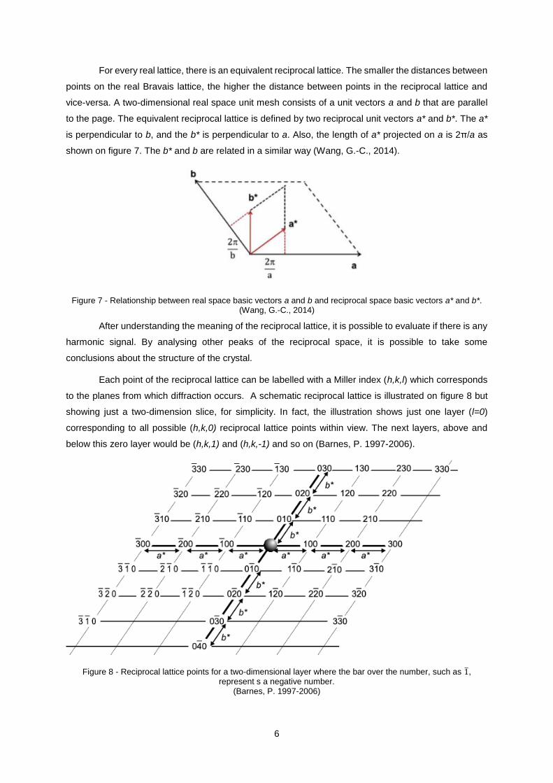
For every real lattice, there is an equivalent reciprocal lattice. The smaller the distances between

points on the real Bravais lattice, the higher the distance between points in the reciprocal lattice and

vice-versa. A two-dimensional real space unit mesh consists of a unit vectors a and b that are parallel

to the page. The equivalent reciprocal lattice is defined by two reciprocal unit vectors a* and b*. The a*

is perpendicular to b, and the b* is perpendicular to a. Also, the length of a* projected on a is 2π/a as

shown on figure 7. The b* and b are related in a similar way (Wang, G.-C., 2014).

Figure 7 - Relationship between real space basic vectors a and b and reciprocal space basic vectors a* and b*. (Wang, G.-C., 2014)

After understanding the meaning of the reciprocal lattice, it is possible to evaluate if there is any

harmonic signal. By analysing other peaks of the reciprocal space, it is possible to take some

conclusions about the structure of the crystal.

Each point of the reciprocal lattice can be labelled with a Miller index (h,k,l) which corresponds

to the planes from which diffraction occurs. A schematic reciprocal lattice is illustrated on figure 8 but

showing just a two-dimension slice, for simplicity. In fact, the illustration shows just one layer (l=0)

corresponding to all possible (h,k,0) reciprocal lattice points within view. The next layers, above and

below this zero layer would be (h,k,1) and (h,k,-1) and so on (Barnes, P. 1997-2006).

Figure 8 - Reciprocal lattice points for a two-dimensional layer where the bar over the number, such as 1̅, represent s a negative number.

(Barnes, P. 1997-2006)

7

To simplify, and since only a two-dimensional system is being studied, the peaks represented

in this work are labelled in form of (h,k). The peaks considered in this work are illustrated in figure 9.

Figure 9 - Representation of a section of a two-dimensional reciprocal lattice and the (1 1) and (2 0) peaks.

As referred before, the hexagonal structure it’s characterized by having a = b and therefore, in

the reciprocal space, a* = b*. If the hexagonal structure is perfect, only one peak will be visible, as the

(01) and (10) points will have the same position value, i.e. same xc value. For the reciprocal space

peaks, their peak position can relate to the (10) peak by the expressions 3 and 4. It’s important to note

that this is only valid for a perfect hexagonal structure where a*=b*.

𝑥𝑐( 1 1 ) = √3 ∙ 𝑥𝑐( 1 0 ) (3)

𝑥𝑐( 2 0 ) = 2 ∙ 𝑥𝑐( 1 0 ) (4)

By confirming if these correlations are applicable to the case in study, it is possible to evaluate

if the structure of the 2D crystal is perfectly hexagonal or if there are any distortions present.

I.7 Experimental Method

I.7.1 Langmuir Film, Langmuir Trough

Langmuir monolayers are monomolecular insoluble films on the surface of a liquid. They are an

excellent model system for studying ordering in two dimensions. The most common surface is water

and the most common monolayers are formed by molecules which have a hydrophilic head and a

hydrophobic tail (Kaganer, V., Mohwald, H., Dutta, P., 1999).

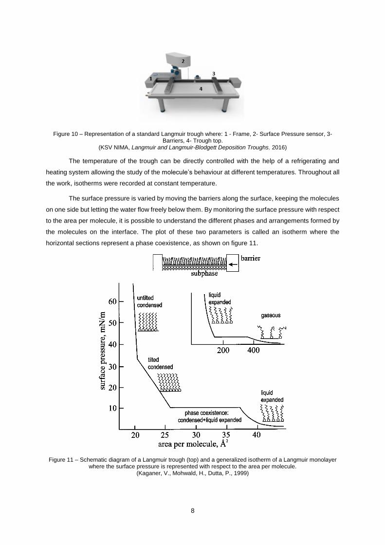
To study these insoluble monolayers, a Langmuir trough is used. As displayed on figure 10,

Langmuir troughs include a set of barriers (3), a Langmuir trough top (4) and a surface pressure sensor

(2) as standard. The trough top, which is often made of hydrophobic material that improves subphase

containment, holds the liquid phase where the monolayers are fabricated. Before creating a monolayer,

the trough top is filled with an aqueous subphase. A monolayer is then created by spreading a solution,

previously prepared with a volatile and water insoluble solvent, on the surface using a syringe. The

monolayer can then be compressed with the help of a set of software-controlled barriers that move at a

designated speed. The surface pressure sensor provides information about monolayer packing density

(KSV NIMA, Langmuir and Langmuir-Blodgett Deposition Troughs, 2016).

8

Figure 10 – Representation of a standard Langmuir trough where: 1 - Frame, 2- Surface Pressure sensor, 3- Barriers, 4- Trough top.

(KSV NIMA, Langmuir and Langmuir-Blodgett Deposition Troughs, 2016)

The temperature of the trough can be directly controlled with the help of a refrigerating and

heating system allowing the study of the molecule’s behaviour at different temperatures. Throughout all

the work, isotherms were recorded at constant temperature.

The surface pressure is varied by moving the barriers along the surface, keeping the molecules

on one side but letting the water flow freely below them. By monitoring the surface pressure with respect

to the area per molecule, it is possible to understand the different phases and arrangements formed by

the molecules on the interface. The plot of these two parameters is called an isotherm where the

horizontal sections represent a phase coexistence, as shown on figure 11.

Figure 11 – Schematic diagram of a Langmuir trough (top) and a generalized isotherm of a Langmuir monolayer where the surface pressure is represented with respect to the area per molecule.

(Kaganer, V., Mohwald, H., Dutta, P., 1999)

9

Throughout the study of isotherms, measurements of structure, area, intermolecular

interactions, phase transitions and compressibility can be taken in order to characterize a certain

compound or mixture (KSV NIMA, Langmuir and Langmuir-Blodgett Deposition Troughs, 2016).

Although Langmuir monolayers have been studied since 1918, it is safe to say that the study

and development of these monolayers is far from concluded as new applications in biophysics and

medicine are being tested.

I.7.2 Brewster Angle Microscopy

Brewster Angle Microscopy was first introduced in 1991 (Hönig, D. 1991), (Hénon, S., 1991).

Since its introduction, it has become the standard technique for the imaging of thin films on liquid

surfaces. This method can be used to relate the BAM images with characteristic phase transition points

in a Langmuir isotherm. This gives valuable information on the formation dynamics of the monolayer.

When a light beam hits a surface, it usually reflects from it. If a p-polarized light beam is directed

at a clean surface at the Brewster angle, no reflection occurs. This behaviour is explained by Brewster’s

law which describes the use of the Brewster angle (α) for a particular optical media with a refractive

index of n (KSV NIMA AN 9, 2016).

tan(𝛼) =𝑛2

𝑛1

(5)

The expression 5 represents the Brewster’s law where α is the Brewster angle, n1 the refractive

index of air (≈1) and n2 the refractive index of water (≈1,33). The Brewster angle for the air-water

interface is approximately 53°, and under this condition the top view image of a pure water surface

appears black as no light is reflected. Addition of material to the air-interface modifies the local refractive

index (RI), and hence, a small amount of light is reflected and displayed within the image. The displayed

image contains areas of varying brightness determined by the particular molecules and packing

densities across the sampling area (KSV NIMA, Brewster Angle Microscopes, 2016). Figures 12 and 13

represent Brewster Angle schemes.

Figure 12 - The principle of Brewster Angle Microscopy.

(KSV NIMA, Brewster Angle Microscopes, 2016).

Figure 13 - Simplified BAM scheme. (adapted from (Lin He, 2015)).

10

I.7.3 Grazing Incidence X-Ray Diffraction and Synchrotron Radiation

X-Rays were discovered by Wilhelm Rontgen, a German physicist in 1895. The X-Ray is

electromagnetic radiation of extremely short wavelength, ranging from about 10-8 to 10-12 m, and high

frequency, from 1016 to 1020 Hertz (Stark, G., 2017).

The Grazing Incidence X-Ray Diffraction, GIXD, was originally developed in 1979 (Marra, W.

C., 1979). In a GIXD experiment, the incident X-Ray beam impinges onto the surface of a film at an

incident angle of 1° or less, and the detector is placed in a horizontal plane parallel to the film surface

to collect diffraction from lattice planes which are perpendicular to the surface, as represented on figure

14 (Huang, T. C.).

Figure 14 - Schematic of the Symmetric GIXD geometry. (adapted from (Huang, T. C.)).

Since the 60’s, of the XX century, some big potentialities for the synchrotron radiation,

concerning the attainment of large range electromagnetic radiations, were being recognized, in

particular the X-Rays. The first synchrotron radiation was observed in 1947 on the General Electric

Laboratories in the United States (Costa, 2004).

In a synchrotron, charged particles, mainly electrons, are accelerated to very high energies in a

linear accelerator and the booster ring to typically billions of electron volts. They are then confined to a

closed orbit, the storage ring, where they circulate in vacuum pipes for several hours, emitting

synchrotron radiation. The emitted light is channelled through beamlines to the experimental stations

where experiments are conducted. Specially designed synchrotron light sources are used worldwide for

X-Ray studies of materials (Stark, G., 2017), (NSRRC, 2010). An example of structure of a synchrotron

is presented on figure 15.

11

Figure 15 – SOLEIL Synchrotron structural scheme. (Celli, F., 2015)

All the experiments were carried out at the SIRIUS beamline in SOLEIL Synchrotron, Orsay,

France. The SIRIUS beamline takes advantage of the best energy range of the SOLEIL synchrotron

ring between 1,4 and 13 keV in order to provide a tool for structural study of not only soft interfaces,

such as air/water interface, Langmuir monolayers, self-assembled organic films and liquid crystal

interfaces, but also semiconductor or magnetic nanostructures such as metal and oxide magnetic

multilayers for example (Fontaine, P., 2014), (Ciatto, G., 2016).

For this study, all diffraction scans were taken at constant temperature and in real time during

compression and expansion of the Langmuir film. The diffraction results obtained were then treated

using the program Origin and later compared with the isotherms and BAM results in order to complement

the study of the fluorinated compounds and mixtures. All the peaks obtained from the X-Ray diffractions

experiments were adjusted individually as exemplified, on figure 16.

Figure 16 - Adjustment of a peak from X-Ray diffraction experiments, using the Lorentz model in Origin program.

13

II. Results and Discussion

II.1 Chemical Compounds and solvents

All the chemical compounds used in the experiment are described in table 2. In order to

understand the influence of fluorinated and hydrogenated molecules, different solutions were prepared

for the mixture of hydrogenated and fluorinated compounds in a vast range of concentrations as shown

in table 3.

Throughout the whole experiment, the solutions were spread on the trough with Hamilton

syringes. Water at 18,2 MΩ·cm from Milli-Q system was used for filling the Langmuir through and

preparing the aqueous subphase and all laboratorial glassware was cleaned using Helmanex®.

Table 2 - Properties of the chemical compounds used in the experiment.

Compound Formula Abbreviation Origin C (mM) Purity

1H,1H-Perfluoro-1-Tetradecanol F(CF2)13CH2OH F14OH Synthesised 0,93 96 %

1H,1H-Perfluoro-1-Octadecanol F(CF2)17CH2OH F18OH Synthesised 1,29 96 %

1-(Perfluoro-n-octyl) tetradecane F(CF2)8(CH2)14H F8H14 Synthesised 1,02 96 %

Perfluorododecanoic Acid C11F23COOH F11COOH Aldrich 1,13 95 %

Myristic Acid C13H27COOH H13COOH Aldrich 1,14 99,5 %

Table 3 - Concentrations of the F11COOH + H13COOH solutions.

Experimental Values Rounded Values

Solution C (mM) % F11COOH

(molar)

% H13COOH

(molar)

% F11COOH

(molar)

% H13COOH

(molar)

1 1,056 18,3 81,7 20 80

2 1,21 35,5 64,5 35 65

3 1,09 58 42 60 40

4 1,17 67,5 32,5 70 30

5 1,17 78,2 21,8 80 20

For solvents, F14OH and F8H14 were dissolved in chloroform and F18OH dissolved in a mixture

of n-hexane/ethanol (3:1; %vol). To take in consideration that the fluorinated alcohols are not very

soluble and the solutions need an ultrasound bath for more than one hour each time they are removed

from the fridge, where they are stored. A consequence of this is a slightly change of pressure value due

to some partial evaporation of solvent stored in the tap of the bottles. The pure F11COOH was dissolved

in a mixture of 90% n-hexane and 10% ethanol (%vol) and the pure H13COOH dissolved in chloroform.

For the solutions of F11COOH + H13COOH, the solvent used was a mixture of 80% n-hexane and 20%

ethanol (%vol).

14

For the mixtures (solutions 1 to 5), F11COOH and H13COOH solutions, a pH=1.0 subphase

was used in order to stabilize the acid. The subphase was achieved by preparing an aqueous solution

using hydrochloric acid.

The solvents used to prepare the spreading solutions and to rinse the syringes and other tools

are described in table 4.

Table 4 - Solvents used in the experiment.

Solvent Formula Origin Purity

Hydrochloric Acid HCl Analar Normapur 37 %

Ethanol C2H6O Analar Normapur 99,86 %

N-Hexane C6H14 Rotipuran 99 %

Chloroform CHCl3 Carlo Erba Reagents 99 %

15

II.2 H13COOH

II.2.1 Isotherms

For the C13H27COOH, also known as H13COOH, a solution of 1,14mM was prepared and

spread in the Langmuir trough, filled with an aqueous acid subphase (pH=1,0).

The first isotherms were recorded at low temperatures to find the value at which the LE phase

is suppressed. It was verified that, at 6°C, the LE phase disappears and the molecules go directly from

gas phase to LC phase, as represented on figure 17.

Figure 17 - Isotherms of pure H13COOH at low temperatures and the disappearance of the LE phase at 6°C.

By recording an isotherm at 22°C it is clear the existence of another phase, the LE phase that

got suppressed at 6°C, which causes the change of slope at 18mN/m. Both isotherms are represented

on figure 18.

Figure 18 - Isotherms of pure H13COOH at 6°C and 22°C.

0

5

10

15

20

25

0 0,2 0,4 0,6 0,8 1

P (

mN

/m)

Area per molecule (nm2/mol)

10°C

7°C

6°C

0

5

10

15

20

25

30

0 0,2 0,4 0,6 0,8 1

P (

mN

/m)


6°C

22°C

16

As shown in figure 18, a plateau at zero pressure is observed for both temperatures at values

of molecular area above 0,4nm2/mol. This plateau represents mainly a gas phase where the molecules

are not organized and the reduction of molecular area doesn’t increase the pressure. At around

0,4nm2/mol there is an increase of pressure caused by the lower value of molecular area that induce

the molecules to become closer.

For the lower temperature, 6°C, the molecules enter a LC phase where, as the pressure

increases, the domains are forcibly tighter packed until a certain pressure is reached causing a collapse.

The pressure of the collapse is around 21mN/m. For the higher temperature, 22°C, the behaviour is

slightly different. After the mainly gas plateau at zero pressure, the molecules enter a LE phase before

reaching the LC phase at around 0,23nm2/mol and 18mN/m. The small plateau at high pressures

represents the coexistence between the LE and LC phase.

This behaviour is in accordance with the literature (Akamatsu,S., Rondelez, F., 1991) that states

that below the triple point temperature T0 (6,6 ± 0,3 °C), the LE phase does not exist, and the gas phase

transforms directly into LC phase. Between T0 and T* (24 ± 0,5 °C) the LE phase transforms into LC1

phase. Upon further compression, there is another transition from LC1 phase to the LC2 phase. This

transition is signalled by a narrow plateau at high pressures which is usually very difficult to distinguish.

Although is not possible to detect the LC1-LC2 phase transition from the isotherm, it is expected that it

happens at pressures above 22mN/m. Above T* there is a direct transition between LE phase and LC2

phase and the LC1-LC2 phase transition disappears.

Another conclusion to take from these isotherms is the compressibility. For 6°C the value of the

compressibility is 21,48 m/N (for the region between 5,5-18,5mN/m) whereas at 22°C is 33,27 m/N (for

the region between 0,95-17,5mN/m). For 22°C the value for the compressibility of the LE phase is in

accordance with the expected since 30 < 33,27 < 60 m/N. The compressibility of the LC phase at 22°C

has a high error percentage since the amount of points is insufficient to guarantee a good adjustment.

Since at 6°C there is only LC phase, the value of compressibility should be between 5 and 10 m/N. The

value of compressibility obtained for the LC phase at 6°C is higher than expected but has a slightly lower

slope than the LC phase at 22°C.

17

II.2.2 BAM images

The pure H13COOH solution was analysed using Brewster Angle microscopy technique at

22°C to better understand the behaviour of the molecules, as represented on figure 19.

Figure 19 - BAM images for pure H13COOH at 22°C.

Although the contrast of the experiment doesn’t lead to better conclusions, it is possible to say

that, at low pressures, there are some isolated domains. At around 16mN/m there is a formation of many

round domains that tend to merge into each other as the pressure increases. When the pressure

reaches higher values, such as 25mN/m, the amount of liquid between domains is so little, that the

round domains are no longer visible, forming a bigger agglomerate that collapses at around 26mN/m.

0

5

10

15

20

25

30

35

0 0,2 0,4 0,6 0,8 1

P (

mN

/m)


18

II.2.3 X-Ray Diffraction

The pure H13COOH was analysed under X-Ray Diffraction technique to determine the peak’s

position, area and width. The experiments were performed at 6°C and 22°C. The diffraction results

obtained at 6°C are represented on figure 20 that shown the variance of the parameter xc according to

the pressure.

Figure 20 - Position of the diffraction peak of pure H13COOH with respect to the pressure at 6°C.

The X-Ray diffraction results at 6°C show the presence of a double peak that, as the pressure

increases, has the tendency to become a single peak. The double peak is the signature for a rectangular

structure, with some possible tilted chains.

At high temperature, only one peak was scanned, for 25mN/m as shown on figure 21. At 22°C

the peak’s position is slightly lower compared with the values obtained at 6°C, with a value of 14,7nm-1.

Figure 21 - X-Ray diffraction result for the pure H13COOH at 22°C.

For further calculations, it was considered that the average peak’s position for the pure

hydrogenated compound, H13COOH, is 15nm-1.

13,5

13,7

13,9

14,1

14,3

14,5

14,7

14,9

15,1

0 5 10 15 20 25

xc (

nm

-1)

P (mN/m)

19

II.3 Fluorinated Compounds

II.3.1 F11COOH

II.3.1.1 Isotherms

For the C11F23COOH, also known as F11COOH, a solution of 1,14mM was prepared and spread

on the Langmuir trough filled with an aqueous subphase (pH=1,0). The isotherms obtained are

represented on figure 22.

Figure 22 - Isotherms of pure F11COOH at 6°C and 22°C.

Due to the presence of fluorinated groups, the initial pressure at deposition is not zero. At high

values of area/molecule, the initial pressure value is around 2,5mN/m caused by the large atomic radius

of the Fluoride molecules deposited.

Isotherms of typical fatty acids usually exhibit three distinct regions, represented in figure 23. As

the mechanical barriers are being closed it is expected a gradual onset of surface pressure. This region

is known as the disordered region where the hydrophobic chains are lifted away from the surface.

Because very weak interactions exist between the water and the tail groups, this region is often referred

as a 2-D gas (Rontu, N., Vaida, V., 2007).

Figure 23 - Molecular orientation at the air/water interface as a function of barrier positions.

Since the fluorinated chains are rigid, the LE state represented in figure 23 does not exist. In

fact, the gas phase transforms directly into a LC phase. When the molecules are spread in the Langmuir

trough, they are in a disordered gas phase. At 22°C, a small plateau is visible beginning at 0,66nm2/mol.

This plateau represents the coexistence between the gas phase and the low energy LC phase.

0

5

10

15

20

25

30

35

0 0,2 0,4 0,6 0,8 1

P (

mN

/m)


6°C

22°C

20

The LC phase is clearly signalled by the sharp increase of the slope. The molecules form a

solid-like arrangement and are in rigid contact with one another. The area/molecule of the liquid in the

LC phase is around 0,3nm2/mol. As the film is compressed beyond the LC region, the collapse occurs

causing the molecular layers to ride on top of each other and form disordered multilayers. The pressure

value of the collapse is around 35mN/m.

As shown before, the triple point temperature for the hydrogenated compound at which the LE

phase disappears is around 6°C. An isotherm at that same temperature was recorded for the pure

F11COOH to assume some coherence in the experiment. The behaviour of the 6°C isotherm is slightly

different from the one recorded at 22°C being the disappearance of the plateau the main difference.

In terms of compressibility, the values obtained for the LC phase were 9,5m/N for 22°C (in the

region between 13,5-34mN/m) and 9,7m/N for 6°C (in the region between 13,8-35,5mN/m). These

values are between 5 m/N and 10 m/N, the range expected for the LC phase.

21

II.3.1.2 BAM images

The pure F11COOH solution was analysed using Brewster Angle microscopy technique at 22°C

to better understand the behaviour of the molecules. Due to the low reflective index of fluorinated chains

(Matsumoto, Y., Nakahara, H. et al, 2007), the contrast is very low making it a difficult task to identify

clearly the domains and phases of the film. The BAM images obtained are presented on figure 24.

Figure 24 - BAM images for pure F11COOH at 22°C.

Although the contrast is very low, many domains are visible during all compression phase.

Ordered domains reflect the emitted light differently than those from a subphase without monolayers.

Thus, ordered domains are visual in brighter contrast than disordered ones due to the difference in

reflectivity between them (Matsumoto, Y., Nakahara, H. et al, 2007). These bright domains are visible

since the beginning of the LC phase, around 0,35nm2/mol, as the molecules are getting more packed

and organized. The number of bright domains increases as the barriers are being compressed and the

pressure increasing, creating more organized domains than in the disordered gas phase.

0

5

10

15

20

25

30

35

0 0,2 0,4 0,6 0,8 1

P (

mN

/m)


22

II.3.1.3 X-Ray Diffraction

The F11COOH was analysed under X-Ray Diffraction technique to determine the peak’s

position, area and width. The experiments were performed at 18°C and 6°C. By plotting the logarithm

of intensity with respect to the peak’s position it is possible to analyse the diffraction spectra for a certain

temperature as represented on figure 25 for 18°C.

Figure 25 - Diffraction spectra for the pure F11COOH at 18°C for different pressures, represented by the logarithm of intensity with respect to the peak position.

The diffraction spectra at 18°C shows that the intensity increases with pressure, specially at

lower values, i.e. below 10mN/m. It is also clear the shift of the peak’s position for higher values as the

pressure increases. That variation of peak’s position is also visible on figure 26 that presents the

variation of peak position, xc, with respect to the pressure.

Figure 26 - Position of the (10) peak of F11COOH with respect to the pressure at 18°C.

12,3

12,35

12,4

12,45

12,5

12,55

15 20 25 30 35 40 45 50

xc (

nm

-1)

P (mN/m)

23

For 6°C, the diffraction spectra is presented on figure 27 where the variation of peak’s position

and intensity is visible.

Figure 27 - Diffraction spectra for the pure F11COOH at 6°C for different pressures, represented by the logarithm of intensity with respect to the peak position.

At 6°C, the peak’s intensity increases with the pressure and the peak’s position for pressures

higher than 10mN/m is slightly higher than for low pressures 3-5mN/m. There is also a shift in peak’s

position even though it is less noticeable than for 18°C. This variation of peak’s position with pressure

is presented on figure 28.

Figure 28 - Position of the (10) peak of F11COOH with respect to the pressure at 6°C.

Just like for 18°C, the peak position values at 6°C follow a linear increase with pressure.

12,3

12,35

12,4

12,45

12,5

12,55

5 10 15 20 25 30 35 40

xc (

nm

-1)

P (mN/m)

24

Taking in consideration the diffraction peaks at 6°C, the ratio between the peak positions, xc,

was calculated to guarantee the existence of a perfect hexagonal structure.

Table 5 - Ratio between F11COOH peak positions at 6°C for different values of pressure.

P (mN/m) xc (11) / xc (10) xc (20) / xc (10)

10 1,731031 1,99894

15 1,731065 1,998315

25 1,730811 1,998192

34,5 1,731397 1,99856

As referred before, the ratio between the peaks from the reciprocal space, xc(1 1) and xc(2 0), and

the xc(1 0) peak can be expressed by the expressions 3 and 4.

𝑥𝑐( 1 1 ) = √3 ∙ 𝑥𝑐( 1 0 ) (3) 𝑥𝑐( 2 0 ) = 2 ∙ 𝑥𝑐( 1 0 ) (4)

By plotting the two ratios previously calculated in order of the pressure, as presented on figure

29, it is safe to say the pure F11COOH has a perfect hexagonal structure as both ratios remain constant

with pressure.

Figure 29 - Ratio between F11COOH peak positions at 6°C with respect to the pressure.

Using the X-Ray diffraction results it is possible to take many more conclusions. One of them is

to estimate the microscopic compressibility and compare it with the one previously calculated by the

isotherm. To estimate the value of microscopic compressibility, the area per molecule is calculated from

the xc parameter using expression 6.

𝐴

𝑚𝑜𝑙𝑒𝑐𝑢𝑙𝑒= (

2𝜋

𝑥𝑐)

2

∙1

cos(𝜋6⁄ )

(6)

1,7

1,75

1,8

1,85

1,9

1,95

2

2,05

0 5 10 15 20 25 30 35 40

Rat

io

P (mN/m)

xc(11) / xc(10)

xc(20) / xc(10)

25

The area per molecule calculated is then plotted with a logarithm scale for different pressures

as represented on figure 30 for 18°C and figure 31 for 6°C.

Figure 30 - Logarithm of area per molecule of F11COOH with respect to the pressure at 18°C.

Taking the linear regression in consideration, the compressibility for pure F11COOH at 18°C is

0,5 m/N (for the region between 20-50mN/m). The compressibility calculated from the isotherm results

is 9,5 m/N which can lead to the conclusion that this last value is from a macroscopic variation compared

to the microscopic one that is recorded in the X-Ray diffraction experiment.

Figure 31 - Logarithm of area per molecule of F11COOH with respect to the pressure at 6°C.

In this case, the compressibility value at 6°C is 0,3 m/N (for the region between 10-35mN/m)

which is much lower than the 9,69 m/N obtained from the isotherm results. This is a confirmation that,

for a microscopic variation, is much harder to compress that when all trough volume is considered in a

macroscopic point of view. Taking this in consideration, the values obtained are in conform with what

was expected.

y = -0,0005x - 1,2078R² = 0,9916

-1,24

-1,235

-1,23

-1,225

-1,22

-1,215

-1,21

15 25 35 45 55ln

(A)

(nm

2 /m

ol)

P (mN/m)

y = -0,0003x - 1,222R² = 0,9987

-1,24

-1,235

-1,23

-1,225

-1,22

-1,215

-1,21

5 10 15 20 25 30 35 40

ln(A

) (n

m2/m

ol)

P (mN/m)

26

II.3.2 F14OH

II.3.2.1 Isotherms

For the F(CF2)13CH2OH, also known as F14OH, a solution of 0,93mM was prepared and spread

on the Langmuir trough. Isotherms were recorded at 14°C and 22°C as shown on figure 32.

Figure 32 - Isotherms of F14OH at 14°C and 22°C

The isotherms obtained experimentally are in accordance with the literature (Teixeira, M., 2014).

Even though there is an 8°C difference between both experiments, the isotherms are very similar. This

is due to the fact that, at these temperatures, there are no major differences in the behaviour of the

molecules. It’s important to mention that, at 14°C, the isotherm is slightly shifted to the left at the

beginning of the lift-off. This is coherent with the literature (Petty, M., 1996) since, for the same value of

pressure, the area/molecule at 14°C is lower than at 22°C. Therefore, for lower temperatures the

isotherms are shifted to the left compared to the ones recorded at higher temperatures.

Since the fluorinated chains are rigid, that causes the gas phase to transform directly into a low

energy LC phase. At approximately zero pressure there is a plateau that represents the coexistence

between gas phase and LC phase. According to the isotherm, the lift-off starts around 0,4nm2/mol and

the monolayer collapses at around 45mN/m.

Since the collapse happens at approximately 0,21nm2/mol, it is believed that both isotherms are

slightly shifted to the left since the value expected is around 0,25nm2/mol (Teixeira, M., 2014). This can

be justified by a possible increase in concentration due to the ultrasound bath that, by taking more than

45 minutes to dissolve the compound, possibly evaporated some solvent.

0

5

10

15

20

25

30

35

40

45

50

0 0,2 0,4 0,6 0,8 1 1,2

Pre

ssu

re (

mN

/m)


22°C

14°C

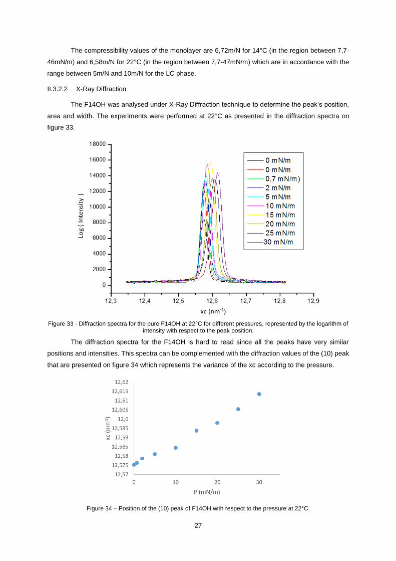
27

The compressibility values of the monolayer are 6,72m/N for 14°C (in the region between 7,7-

46mN/m) and 6,58m/N for 22°C (in the region between 7,7-47mN/m) which are in accordance with the

range between 5m/N and 10m/N for the LC phase.


The F14OH was analysed under X-Ray Diffraction technique to determine the peak’s position,

area and width. The experiments were performed at 22°C as presented in the diffraction spectra on

figure 33.

Figure 33 - Diffraction spectra for the pure F14OH at 22°C for different pressures, represented by the logarithm of intensity with respect to the peak position.

The diffraction spectra for the F14OH is hard to read since all the peaks have very similar

positions and intensities. This spectra can be complemented with the diffraction values of the (10) peak

that are presented on figure 34 which represents the variance of the xc according to the pressure.

Figure 34 – Position of the (10) peak of F14OH with respect to the pressure at 22°C.

12,57

12,575

12,58

12,585

12,59

12,595

12,6

12,605

12,61

12,615

12,62

0 10 20 30

xc (

nm

-1)

P (mN/m)

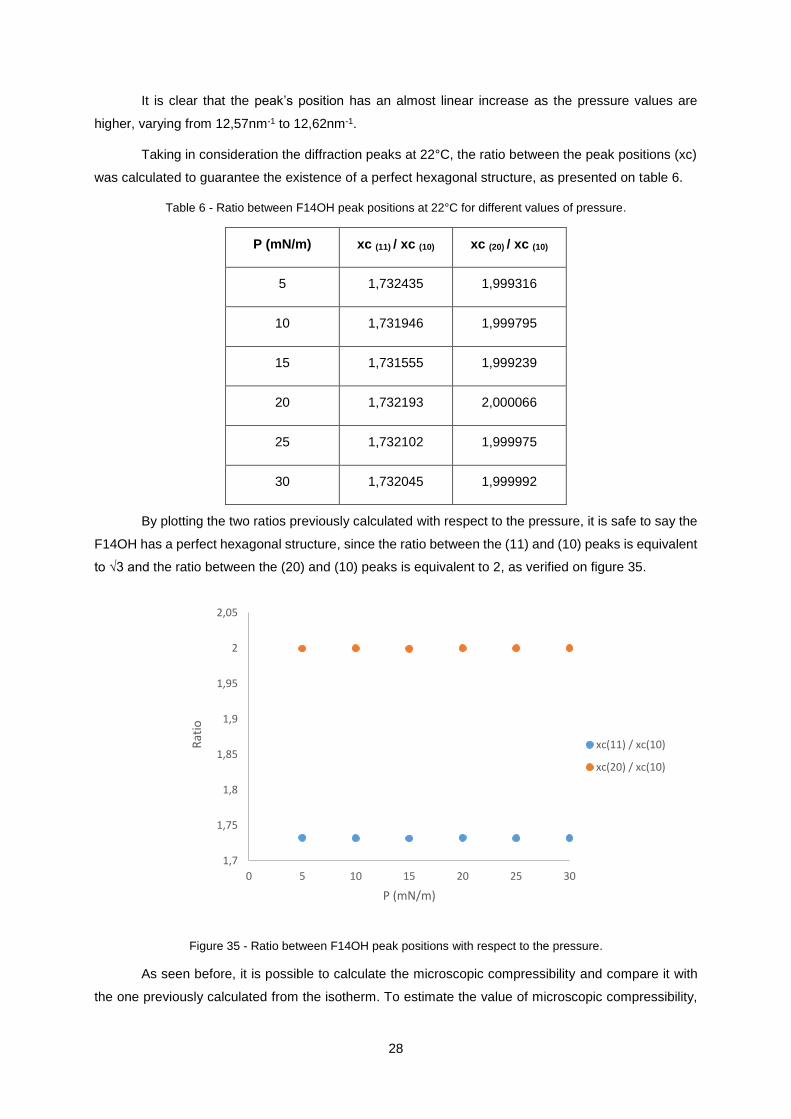
28

It is clear that the peak’s position has an almost linear increase as the pressure values are

higher, varying from 12,57nm-1 to 12,62nm-1.

Taking in consideration the diffraction peaks at 22°C, the ratio between the peak positions (xc)

was calculated to guarantee the existence of a perfect hexagonal structure, as presented on table 6.

Table 6 - Ratio between F14OH peak positions at 22°C for different values of pressure.

P (mN/m) xc (11) / xc (10) xc (20) / xc (10)

5 1,732435 1,999316

10 1,731946 1,999795

15 1,731555 1,999239

20 1,732193 2,000066

25 1,732102 1,999975

30 1,732045 1,999992

By plotting the two ratios previously calculated with respect to the pressure, it is safe to say the

F14OH has a perfect hexagonal structure, since the ratio between the (11) and (10) peaks is equivalent

to √3 and the ratio between the (20) and (10) peaks is equivalent to 2, as verified on figure 35.

Figure 35 - Ratio between F14OH peak positions with respect to the pressure.

As seen before, it is possible to calculate the microscopic compressibility and compare it with

the one previously calculated from the isotherm. To estimate the value of microscopic compressibility,

1,7

1,75

1,8

1,85

1,9

1,95

2

2,05

0 5 10 15 20 25 30

Rat

io

P (mN/m)

xc(11) / xc(10)

xc(20) / xc(10)

29

the area per molecule is calculated from the xc parameter using expression 6 and then plotted with a

logarithm scale as shown on figure 36.

Figure 36 - Logarithm of area per molecule of F14OH with respect to the pressure at 22°C.

The microscopic compressibility of F14OH is 0,19m/N (for the region between 0-30mN/m). This

value is much lower than the 6,58 m/N calculated from the isotherm results as that represents the

macroscopic variation obtained from compression of the mechanical barriers.

The X-Ray diffraction results provide a wide range of information useful to understand the

behaviour of molecules and all their phases. Using the intensity results from F14OH at 22°C and the

area per molecule recorded during the experiment it is possible to estimate the beginning of the plateau,

as represented on figure 37. With the linear regression expression, it is possible to calculate the value

for which the intensity is zero, i.e. the beginning of the plateau.

Figure 37 - Intensity with respect to the area per molecule for the plateau of the isotherm at 22°C.

y = -0,00019x - 1,24381R² = 0,98989

-1,255

-1,253

-1,251

-1,249

-1,247

-1,245

-1,243

-1,241 0 5 10 15 20 25 30 35

ln(A

) (n

m2 /

mo

l)

P (mN/m)

y = -1280,4x + 1023,9R² = 0,9846

0

100

200

300

400

500

600

0,3 0,4 0,5 0,6 0,7 0,8

Inte

nsi

ty (

a.u

.)


30

The value obtained for the beginning of the plateau is 0,8nm2/mol. By zooming in the isotherm

obtained it is possible to conclude the plateau begins around 0,96nm2/mol, as shown in figure 38. That

represents a 16,7% error between the value calculated and the one obtained experimentally.

Figure 38 - Beginning of the plateau obtained experimentally for F14OH at 22°C.

II.3.3 F18OH

II.3.3.1 Isotherms

For the F(CF2)17CH2OH, also known as F18OH, a solution of 1,29mM was prepared and spread

on the Langmuir trough. Isotherms were recorded at 14°C and 22°C as shown on figure 39.

Figure 39 - Isotherms of F18OH at 14°C and 22°C.

The isotherms obtained experimentally are in accordance with the literature (Teixeira, M., 2014).

The behaviour recorded in this isotherm is similar to the one obtained for the F14OH. Both fluorinated

alcohols have only one phase transition from gas phase to LC phase. The plateau at low pressure

0

0,1

0,2

0,3

0,4

0,5

0,6

0 0,2 0,4 0,6 0,8 1 1,2 1,4

P (

mN

/m)


-1

9

19

29

39

49

59

69

0 0,2 0,4 0,6 0,8 1 1,2 1,4

Pre

ssu

re (

mN

/m)


14 ºC

22 ºC

31

represents the region of equilibrium and coexistence between the gas phase and the LC phase. The

region of high surface density corresponds to the condensed monolayer that begins when the slope

changes drastically at around 0,3nm2/mol. Around 45mN/m there is a change in the slope that

represents the collapse of the monolayer.

The isotherm at 14°C is slightly shifted to the left, phenomena also verified for the F14OH and

coherent with the literature (Petty, M., 1996).

In terms of compressibility, the values are 7,17m/N for 14°C (in the region between 8,5-45mN/m)

and 8,5m/N for 22°C (in the region between 8,7-47mN/m) which are in accordance with the range

between 5m/N and 10m/N expected for the LC phase.


The F18OH was analysed under X-Ray Diffraction technique to determine the peak’s position,

area and width. The experiments were performed at 18°C as shown in the diffraction spectra on figure

40.

Figure 40 - Diffraction spectra for the pure F18OH at 18°C for different pressures, represented by the logarithm of intensity with respect to the peak position.

By analysing the diffraction spectra, it is clear there is a double peak for pressures below

10mN/m. The reason of appearance of this double peak is unknown but can possibly be justified by the

existence of tilted molecules. As the pressure increases, the molecules get more packed and only one

diffraction peak is generated. For pressures higher than 20mN/m, the variation is not significant, being

the xc value around 12,647nm-1.

The variation of peak position is also visible on figure 41 which represents the variance of the

parameter xc according to the pressure.

32

Figure 41 – Position of the (10) peak of F18OH with respect to the pressure at 18°C.

The variation of xc in terms of the pressure doesn’t follow a linear regression like it did on the

F14OH, not only because of the existence of a double peak but also due to the incoherent shift to lower

peak position value at 30mN/m.

Taking in consideration the diffraction peaks at 18°C, the ratio between the peak positions (xc)

was calculated to guarantee the existence of a perfect hexagonal structure, as presented on table 7.

Table 7 - Ratio between F18OH peak positions at 18°C for different values of pressure.

P (mN/m) xc (11) / xc (10) xc (20) / xc (10)

10 1,731278 1,999485

10 1,723404 1,991315

20,5 1,730113 1,9983

30 1,730988 1,997921

35 1,731494 1,997814

By plotting the two ratios previously calculated with respect to the pressure, it is safe to say the

F18OH has a perfect hexagonal structure, since the ratio between the (11) and (10) peaks is equivalent

to √3 and the ratio between the (20) and (10) peaks is equivalent to 2 as verified o figure 42.

12,6

12,61

12,62

12,63

12,64

12,65

12,66

12,67

12,68

0 10 20 30 40

xc (

nm

-1)

P (mN/m)

33

Figure 42 - Ratio between F18OH peak positions with respect to the pressure.

For the pressure value of 10mN/m there is a double peak. This double peak can be analysed in

order to understand what causes it to appear at this value of pressure. One way to understand this

behaviour is to compare the value of xc of the double (10) peak with the values obtained for the

reciprocal space peaks recorded on the X-Ray diffraction experiment. The table 8 shows the different

peak’s positions recorded at 10mN/m. These peaks are related with each other, as shown before, by

expressions 3 and 4.

Table 8 - X-Ray diffraction peaks for F18OH at 18°C and 10mN/m.

xc (1 0) (nm-1) xc (1 1) (nm-1) xc (2 0) (nm-1)

12,614 21,838 25,222

12,666 --- ---

For the two (1 0) peaks recorded at 10mN/m, only one (1 1) and (2 0) peaks were discovered.

As verified in table 8, the (1 1) and (2 0) peaks recorded correspond to the first (1 0) peak. The second

(1 0) peak, of value 12,666 nm-1, doesn’t have the harmonics recorded on the X-Ray experiment. This

can be justified by, either the intensity is too low to be visible on the X-Ray, or the structure is not

perfectly hexagonal and so the parameters have different correlations between them which leads to

different xc values that were not scanned in this experiment.

This double peak disappears for pressures higher than 10mN/m, at which the peaks follow the

relations given by expressions 3 and 4.

Just like for F14OH, the logarithm of area per molecule was plotted to estimate the value of

microscopic compressibility. Since there are double peaks in the F18OH X-Ray diffraction results, the

area per molecule was calculated from the “a” and “b” network parameters. Those parameters were

1,7

1,75

1,8

1,85

1,9

1,95

2

2,05

0 10 20 30

Rat

io

P (mN/m)

xc(11) / xc(10)

xc(20) / xc(10)

34

calculated via a computer program that used the xc values as input. The parameters “a” and “b”

correspond to the sides of the rectangle since the sides of the rhombus are the same length as the

smallest diagonal as shown in figure 43.

Figure 43 - Relation between the "a" and "b" network parameters.

Since the rectangle contains the equivalent to two molecules, it’s necessary to take that in

consideration when calculating the area per molecule using expression 7.

𝐴

𝑚𝑜𝑙𝑒𝑐𝑢𝑙𝑒=

𝑎 × 𝑏

2 (7)

As seen before, the area per molecule is plotted with a logarithm scale as presented on figure

44.

Figure 44 - Logarithm of area per molecule of F18OH with respect to the pressure at 18°C.

The microscopic compressibility of F18OH at 18°C is 0,12 m/N (for the region between 0-

35mN/m). This value is much lower than the 8,5 m/N obtained from the isotherm results as that

represents the macroscopic variation obtained from compression of the mechanical barriers.

y = -0,00012x - 1,25194R² = 0,69952

-1,26

-1,258

-1,256

-1,254

-1,252

-1,25

0 10 20 30 40

ln(A

) (n

m2/m

ol)

P (mN/m)

35

II.4 Mixture

II.4.1 F11COOH and F18OH

To better understand the behaviour of these molecules, an experiment at 18°C was performed

by spreading both compounds in the trough using the co-deposition technique. With an acid subphase

(pH=1,0), 85μL of F11COOH and 75μL of F18OH were deposited in the trough. These volumes were

taken from the previously prepared solutions of pure F11COOH and pure F18OH.

An interesting approach to take in consideration is plotting the evolution of the peak’s intensity

for each value of peak position, i.e. a diffraction spectra as shown on figure 45. It is important to note

that the intensity was plotted using a logarithm scale in order to compact the curves and provide a better

visual understanding.

Figure 45 - Diffraction spectra for the F11COOH + F18OH mixture at 18°C for different pressures, represented by

the logarithm of intensity with respect to the peak position.

By analysing the curves for each pressure, it is safe to say that there are two distinct peaks at

different xc values. The peak at lower xc value, around 12,4nm-1, is a single peak and corresponds to

the F11COOH compound. The peak at higher xc value, around 12,65nm-1, is actually a double peak

and represents the F18OH. For lower values of pressure, under 10mN/m, the intensity is unstable and

assumes a constant value for pressure values higher than 10mN/m.

Another thing to take in consideration is the difference between intensities. The intensity of the

fluorinated alcohol is much higher than the one recorded for the F11COOH. This is probably related to

the size of the molecular chains, being the longer chain the one that generates a higher intensity value.

36

By treating the results obtained, the position of the (1 0) peak was plotted for different values of

pressure as shown on figure 46.

Figure 46 – Position of the (10) peak of F11COOH and F18OH co-deposition with respect to the pressure at

18°C.

By analyzing the X-Ray diffraction results, it is possible to conclude that there is complete

segregation of the pure fluorinated compound and the alcohol as there are three complete different

peaks visible for each pressure. The single peak at around 12,42nm-1 represents the F11COOH and

the double peak at higher values represents the fluorinated alcohol F18OH. These results are in

accordance with what was obtained individually for each compound.

12,4

12,45

12,5

12,55

12,6

12,65

12,7

0 5 10 15 20 25

xc (

nm

-1)

P (mN/m)

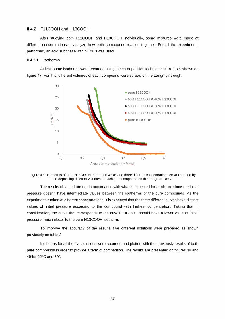
37

II.4.2 F11COOH and H13COOH

After studying both F11COOH and H13COOH individually, some mixtures were made at

different concentrations to analyze how both compounds reacted together. For all the experiments

performed, an acid subphase with pH=1,0 was used.

II.4.2.1 Isotherms

At first, some isotherms were recorded using the co-deposition technique at 18°C, as shown on

figure 47. For this, different volumes of each compound were spread on the Langmuir trough.

Figure 47 - Isotherms of pure H13COOH, pure F11COOH and three different concentrations (%vol) created by

co-depositing different volumes of each pure compound on the trough at 18°C.

The results obtained are not in accordance with what is expected for a mixture since the initial

pressure doesn’t have intermediate values between the isotherms of the pure compounds. As the

experiment is taken at different concentrations, it is expected that the three different curves have distinct

values of initial pressure according to the compound with highest concentration. Taking that in

consideration, the curve that corresponds to the 60% H13COOH should have a lower value of initial

pressure, much closer to the pure H13COOH isotherm.

To improve the accuracy of the results, five different solutions were prepared as shown

previously on table 3.

Isotherms for all the five solutions were recorded and plotted with the previously results of both

pure compounds in order to provide a term of comparison. The results are presented on figures 48 and

49 for 22°C and 6°C.

0

5

10

15

20

25

30

0,1 0,2 0,3 0,4 0,5 0,6

P (

mN

/m)


pure F11COOH

60% F11COOH & 40% H13COOH



pure H13COOH

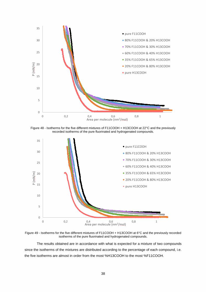
38

Figure 48 - Isotherms for the five different mixtures of F11COOH + H13COOH at 22°C and the previously recorded isotherms of the pure fluorinated and hydrogenated compounds.

Figure 49 - Isotherms for the five different mixtures of F11COOH + H13COOH at 6°C and the previously recorded isotherms of the pure fluorinated and hydrogenated compounds.

The results obtained are in accordance with what is expected for a mixture of two compounds

since the isotherms of the mixtures are distributed according to the percentage of each compound, i.e.

the five isotherms are almost in order from the most %H13COOH to the most %F11COOH.

0

5

10

15

20

25

30

35

0 0,2 0,4 0,6 0,8 1

P (

mN

/m)


pure F11COOH






pure H13COOH

0

5

10

15

20

25

30

35

0 0,2 0,4 0,6 0,8 1

P (

mN

/m)


pure F11COOH






pure H13COOH

39

There are some conclusions to take from the isotherms recorded at 22°C. As the percentage of

F11COOH in the mixture increases, there is a change of slope at low pressure which is in accordance

with what was obtained for the pure F11COOH isotherm. There is also an increase of slope at high

pressures that ends with the collapse around 35mN/m. For the mixture with highest percentage of

H13COOH, there is a change of phase around 25mN/m expressed by a variation of slope.

At 6°C, although the LE phase of the pure H13COOH is supressed, the behaviour of the five

mixtures is slightly different. The molecules of hydrogenated compound, under certain conditions, may

not hold the perfect hexagonal structure and therefore induce a LE phase. This can happen if a

fluorinated molecule enters the previously formed hydrogenated structure, preventing it from remaining

perfectly hexagonal, as shown on figure 50. The main differences are visible for the isotherms of the

mixtures with higher percentage of hydrogenated compound. As the percentage of hydrogenated

decreases, the isotherm starts to behave more like the pure F11COOH by having no LE phase.

Figure 50 - Example of a perfect hexagonal structure, on the left, formed by hydrogenated molecules followed by a non-perfect hexagonal structure, on the right, formed by hydrogenated molecules and one fluorinated molecule,

with a higher atomic radius.

To better understand the difference in slope according to the percentage of each compound,

the compressibility values for every mixture were calculated and compared with the compressibility of

the pure compounds, as shown on table 9.

Table 9 - Compressibility values for the five mixtures and pure compounds at 22°C and 6°C with the correspondent regions between which the compressibility was calculated.

Solution Compressibility

at 22°C (m/N)

Region (mN/m)

Compressibility at 6°C (m/N)

Region (mN/m)

Pure F11COOH 9,5 13,5-34 9,69 13,8-35,5

80% F11COOH & 20% H13COOH 12,86 14-30,5 12,74 13-37

70% F11COOH & 30% H13COOH 12,93 14-30 11,23 12-35

60% F11COOH & 40% H13COOH 18,85 12-24 13,83 11,5-31,5

35% F11COOH & 65% H13COOH 20,39 9,7-32 10,34 14,5-40

20% F11COOH & 80% H13COOH 21,29 8,2-25 20,98 9-26

Pure H13COOH 33,27 0,95-17,5 21,48 5,5-18,5

40

It’s important to note that the compressibility value calculated for the pure H13COOH

corresponds to the LE phase since there were not enough points to provide a good adjustment of the

LC phase. By analysing the results from table 9, it is clear the compressibility value at 22°C decreases

as the percentage of F11COOH increases. This is in accordance with what is expected because the

more fluorinated molecules present in a mixture, the more that mixture resembles with the pure

F11COOH solution. At 6°C that relation is not so clear as the values vary a lot and that variation is not

in accordance with the change in concentration. This variation is better expressed on figures 51 and 52.

Figure 51 - Relation between the compressibility values calculated from the isotherms at 22°C and the percentage

of F11COOH on the mixtures.

Figure 52 - Relation between the compressibility values calculated from the isotherms at 6°C and the percentage of F11COOH on the mixtures.

0

5

10

15

20

25

30

35

0 20 40 60 80 100

Co

mp

ress

ibili

ty (

m/N

)

% F11COOH (%molar)

0

5

10

15

20

25

0 20 40 60 80 100

Co

mp

ress

ibili

ty (

m/N

)

% F11COOH (%molar)

41

II.4.2.2 BAM images

Some Brewster Angle Microscopy experiments were conducted to better understand the

behaviour of the F11COOH + H13COOH mixture. As explained before, the fluorinated molecules are

not very visible due to their low reflective index. Because of that, only the 20%F11COOH &

80%H13COOH mixture was carefully analysed as well as the 70%F11COOH & 30%H13COOH for

comparison. The reason why the mixture with higher percentage of fluorinated was not used for BAM

experiments is because the percentage of F11COOH is so high that wouldn’t allow the results to be

clearly visible. Instead, the second mixture with highest fluorinated percentage was used.


The 20%F11COOH & 80%H13COOH mixture was analysed at three different temperatures,

22°C, 14°C and 6°C. Firstly, the BAM images at 22°C are presented on figure 53.

Figure 53 - BAM images for the 20%F11COOH & 80%H13COOH mixture at 22°C.

By analysing the results obtained from the BAM experiment, it is possible to conclude that, at

very low pressures, there is mainly only gas phase which is characterized by the inexistence of visible

domains. As the pressure increases, some bright domains of liquid start to appear. These domains are

0

5

10

15

20

25

30

35

0 0,2 0,4 0,6 0,8 1

P (

mN

/m)


42

mainly rich in H13COOH as that is the compound in higher percentage. At very high pressure, around

35mN/m, there is a very disorganized phase of hydrogenated compound that collapses shortly after.

Secondly, the BAM images at 14°C are presented on figure 54.


It is important to note that the dashed line corresponds to an image taken during expansion

phase while the full line represents the images taken on the regular compression phase.

At 14°C the suppression of the gas phase happens at lower pressure, around 15mN/m rather

than the 25mN/m result at 22°C. Just like for 22°C, there are many liquid domains visible at low

pressures. Around 18mN/m some bigger domains appear, getting more organized as the pressure

increases. At 37mN/m there are a few 2D domains visible but those formations are more noticeable

when the expansion begins and, around 14mN/m, a mixture of bright domains and some 2D structures

-1

4

9

14

19

24

29

34

0 0,2 0,4 0,6 0,8 1 1,2

P (

mN

/m)


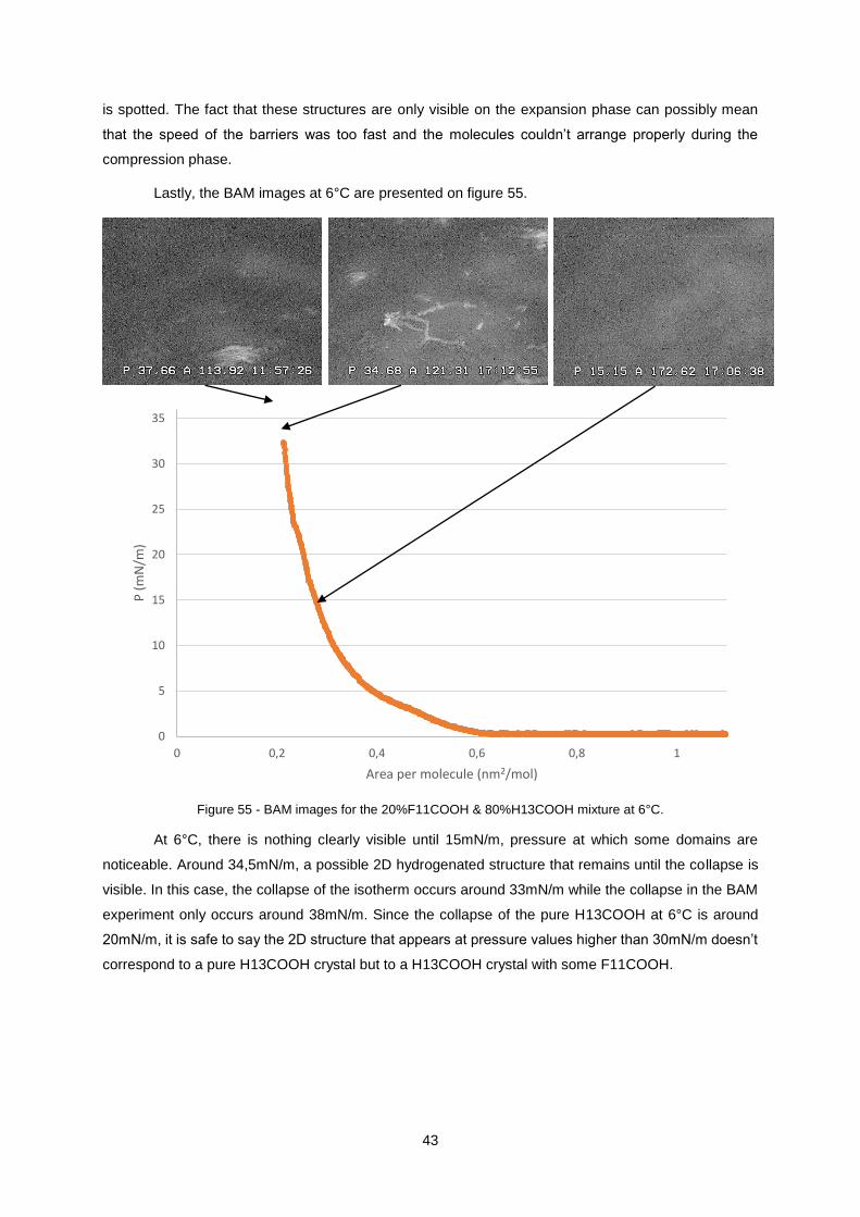
43

is spotted. The fact that these structures are only visible on the expansion phase can possibly mean

that the speed of the barriers was too fast and the molecules couldn’t arrange properly during the

compression phase.

Lastly, the BAM images at 6°C are presented on figure 55.


At 6°C, there is nothing clearly visible until 15mN/m, pressure at which some domains are

noticeable. Around 34,5mN/m, a possible 2D hydrogenated structure that remains until the collapse is

visible. In this case, the collapse of the isotherm occurs around 33mN/m while the collapse in the BAM

experiment only occurs around 38mN/m. Since the collapse of the pure H13COOH at 6°C is around

20mN/m, it is safe to say the 2D structure that appears at pressure values higher than 30mN/m doesn’t

correspond to a pure H13COOH crystal but to a H13COOH crystal with some F11COOH.

0

5

10

15

20

25

30

35

0 0,2 0,4 0,6 0,8 1

P (

mN

/m)


44


The 70%F11COOH & 30%H13COOH mixture was studied under Brewster Angle Microscopy

at 22°C and 6°C. Firstly, the BAM images at 22°C are presented on figure 56.


For this mixture, it is not expected to see clearly many domains since the compound in higher

percentage is the fluorinated, which as a low reflective index. Despite that, during all the compression

there are some isolated liquid domains visible. Around 30mN/m there is a higher number of domains

that are no longer visible when the pressure increases until 33mN/m.

Lastly, the BAM images at 6°C are presented on figure 57.

0

5

10

15

20

25

30

35

40

0 0,2 0,4 0,6 0,8 1

P (

mN

/m)


45


At 6°C, the differences from the 22°C results are not very accentuated. At low pressures, there

is mainly only gas phase and nothing is clearly visible. Around 10mN/m some bright and big domains,

that remain until higher values of pressure, are noticeable. At very high values of pressure, around

43mN/m, there are no domains visible just like at 22°C. This can be due to the fact that, at this pressure,

the hydrogenated molecules have already collapsed.


Many X-Ray diffraction experiments were made for most mixtures at different temperatures to

better understand the influence of each compound, F11COOH and H13COOH.


The mixture with lower percentage of fluorinated compound was analysed under X-Ray

diffraction at 22°C, 14°C and 6°C.

Firstly, the results at 22°C are presented. By plotting the intensity with respect to the peak’s

position it is possible to analyse the diffraction spectra represented on figure 58.

0

5

10

15

20

25

30

35

40

0 0,2 0,4 0,6 0,8 1

P (

mN

/m)


46

Figure 58 - Diffraction spectra for the 20%F11COOH & 80%H13COOH mixture at 22°C for different pressures, represented by the logarithm of intensity with respect to the peak position.

By analysing the diffraction spectra, it is possible to conclude that the intensity of the peak

increases with the pressure. Since the variation of the peak’s position is not clear on the diffraction

spectra, the diffraction results were plotted with the peak’s position and width with respect to the

pressure, as shown on figures 59 and 60.

Figure 59 - Position of the peak of 20%F11COOH & 80%H13COOH mixture with respect to the pressure

at 22°C.


at 22°C.

By analysing the results obtained and comparing them with the results from the pure

compounds, it is possible to admit that around 12,6nm-1 there is a separation between the fluorinated

type molecules and the hydrogenated type. It is possible to estimate the percentage of each compound

in the crystal by using the expressions 8 and 9.

12

12,2

12,4

12,6

12,8

13

13,2

0 5 10 15 20 25 30 35 40

xc (

nm

-1)

P (mN/m)

2

2,5

3

3,5

4

4,5

5

5,5

6

0 5 10 15 20 25 30 35 40

w (

nm

-1)

P (mN/m)

47

𝑆 = (2 𝜋

𝑥𝑐)

2

∙1

cos(30°) (8)

𝑆𝑛 = 𝑥𝑆𝐹 + (1 − 𝑥)𝑆𝐻 (9)

Firstly, it is necessary to calculate the values of the pure compounds so the expression 9 can

be properly used. Using the expression 8 with the xc values of 12,5nm-1 for the F11COOH and 15m-1

for the H13COOH, the SF (0,292nm2) and the SH (0,202nm2) values are obtained. Following the same

method for the peak at 35mN/m with a xc value of 13,06nm-1, a Sn of 0,2672nm2 is obtained which

corresponds to approximately 70% of F11COOH. By multiplying the remaining percentage

corresponding to the H13COOH with the total amount of F11COOH present in the mixture it is possible

to conclude that a total of 6% of hydrogenated type molecules are in the rich fluorinated phase.

0,30 ∗ 20 = 6% 𝑜𝑓 ℎ𝑦𝑑𝑟𝑜𝑔𝑒𝑛𝑎𝑡𝑒𝑑

That phase could be a crystal but, since the peaks are very broad, it is admitted to be just a

phase with both compounds rather than a crystal. By subtracting this percentage from the 80% of

H13COOH existent in the mixture, it is possible to estimate that 74% of H13COOH doesn’t give signal

and, therefore, remains on the LE phase. At this pressure, there is a coexistence between a fluorinated

liquid and a disorganized hydrogenated liquid.

Secondly, the diffraction spectra at 14°C, represented in figure 61, was analysed.


Contrary to the results obtained at 22°C, at 14°C there is a clear separation between the peaks

that correspond to a fluorinated rich phase or to a hydrogenated rich phase. The existence of both

fluorinated peak and hydrogenated peak for pressures higher than 20mN/m is clear on the diffraction

spectra as the fluorinated peak appears around 12,5nm-1 while the hydrogenated one appears around

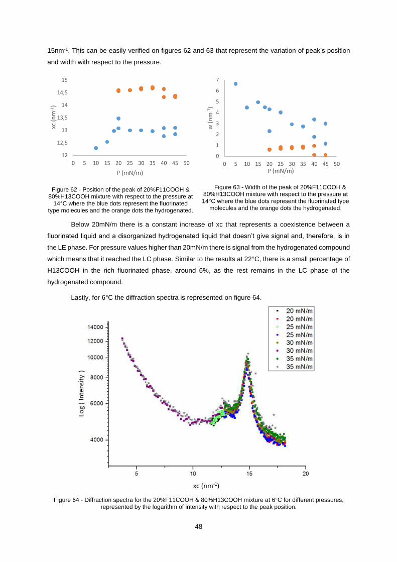
48

15nm-1. This can be easily verified on figures 62 and 63 that represent the variation of peak’s position

and width with respect to the pressure.

Figure 62 - Position of the peak of 20%F11COOH & 80%H13COOH mixture with respect to the pressure at

14°C where the blue dots represent the fluorinated type molecules and the orange dots the hydrogenated.

Figure 63 - Width of the peak of 20%F11COOH & 80%H13COOH mixture with respect to the pressure at 14°C where the blue dots represent the fluorinated type

molecules and the orange dots the hydrogenated.

Below 20mN/m there is a constant increase of xc that represents a coexistence between a

fluorinated liquid and a disorganized hydrogenated liquid that doesn’t give signal and, therefore, is in

the LE phase. For pressure values higher than 20mN/m there is signal from the hydrogenated compound

which means that it reached the LC phase. Similar to the results at 22°C, there is a small percentage of

H13COOH in the rich fluorinated phase, around 6%, as the rest remains in the LC phase of the

hydrogenated compound.

Lastly, for 6°C the diffraction spectra is represented on figure 64.


12

12,5

13

13,5

14

14,5

15

0 5 10 15 20 25 30 35 40 45 50

xc (

nm

-1)

P (mN/m)

0

1

2

3

4

5

6

7

0 5 10 15 20 25 30 35 40 45 50

w (

nm

-1)

P (mN/m)

49

At this temperature, there is also a clear separation between the fluorinated peak, at lower xc

value, and the hydrogenated peak at higher xc value. Since the diffraction spectra was only recorded

for pressures higher than 20mN/m there is no clear change in the intensity as it is almost constant with

pressure. To better understand this, the results obtained are displayed on figures 65 and 66 that

represent the variation of peak’s position and width with respect to the pressure.

Figure 65 - Position of the peak of 20%F11COOH & 80%H13COOH mixture with respect to the pressure at 6°C where the blue dots represent the fluorinated

type molecules and the orange dots the hydrogenated.

Figure 66 - Width of the peak of 20%F11COOH & 80%H13COOH mixture with respect to the pressure at 6°C where the blue dots represent the fluorinated


There is a coexistence of both LC fluorinated and LC hydrogenated phases for values of

pressure between 20mN/m and 35mN/m. Since the width value is rather low, there is a possibility that

the hydrogenated phase is a crystal with some amount of F11COOH. This amount is probably very low

since the xc value at high pressures is almost 15nm-1, which means that, as the pressure increases, the

hydrogenated formations are getting more organized and expelling the fluorinated molecules.

12,5

13

13,5

14

14,5

15

15 20 25 30 35 40

xc (

nm

-1)

P (mN/m)

0,5

1

1,5

2

2,5

3

3,5

4

4,5

5

15 20 25 30 35 40w

(n

m-1

)P (mN/m)

50


The 35%F11COOH & 65%H13COOH mixture was analysed under X-Ray diffraction at 22°C

and 6°C. Firstly, the results at 22°C are presented in the diffraction spectra on figure 67.


By analysing the diffraction spectra, it is clear that there is only a fluorinated peak until 30mN/m

and, for pressures higher than 35mN/m there is an appearance of a hydrogenated peak. This is more

visible on figures 68 and 69 where the variation of peak’s position and width with respect to the pressure

is shown.

Figure 68 - Position of the peak of 35%F11COOH & 65%H13COOH mixture with respect to the pressure


hydrogenated.



hydrogenated.

11

11,5

12

12,5

13

13,5

14

14,5

5 10 15 20 25 30 35 40 45

xc (

nm

-1)

P (mN/m)

0

0,5

1

1,5

2

2,5

3

3,5

4

4,5

5 10 15 20 25 30 35 40 45

w (

nm

-1)

P (mN/m)

51

There is a clear transition of the fluorinated type molecules as the xc value increases with the

pressure until it reaches a constant value. For pressures lower than 35mN/m the molecules are on a

rich fluorinated liquid phase and, at 35mN/m, they enter a LC phase. Just like for the previous mixture,

it is possible to estimate the amount of H13COOH on the fluorinated crystal present above 12,5nm-1.

For 30mN/m and 12,665nm-1, some hydrogenated molecules are present on the fluorinated crystal and

that amount can be estimated using expressions 8 and 9. The Sn value of 0,2841nm2 is obtained which

corresponds to approximately 90% of F11COOH and, following the same logic as before, 3,5% of

H13COOH present on the fluorinated rich crystal. This formation is either not a crystal since the width

values are high or it is a crystal with very small dimensions. For high values of pressure, above 35mN/m,

there is a fluorinated LC phase as well as a hydrogenated LC phase, this one represented by the orange

dots with high values of peak position, around 14,5nm-1.

Lastly, the diffraction spectra at 6°C obtained from the X-Ray diffraction experiment is

represented on figure 70.


By analysing the diffraction spectra at 6°C, the increasing intensity of the fluorinated peaks with

pressure and the shift of the hydrogenated xc values are visible. The fluorinated peak, at 12,5nm-1

doesn’t change position throughout all experiment but the peak’s intensity increases with the pressure.

For the hydrogenated peaks, their position shifts to lower values as the pressure increases until the

molecules collapse around 45mN/m as shown on figure 71.

52

Figure 71 - Representation of the moment of the collapse for the 35%F11COOH & 65%H13COOH at 45mN/m.

All this peak’s position variations with pressure are better represented on figure 72. The variation

of width with the pressure is represented on figure 73.

Figure 72 - Position of the peak of 35%F11COOH & 65%H13COOH mixture with respect to the pressure at 6°C where the blue dots represent the fluorinated




By analysing the results obtained, it is possible to conclude the existence of three distinct

phases. For pressures lower than 15mN/m there is a rich fluorinated LC phase for a peak position of

12,5nm-1. As the pressure increases the H13COOH enters a LC phase that coexists with the LC phase

of the fluorinated compound but, for pressures higher than 25mN/m, that balance changes. The

fluorinated chains start to enter the hydrogenated phase and that causes the xc values to decrease.

That decrease corresponds to a percentage of fluorinated compound that can be estimated using

expressions 8 and 9. For 38mN/m and 14,76nm-1 the Sn value of 0,209nm2 is obtained which

corresponds to approximately 8%F11COOH on the hydrogenated crystal. The width of the

hydrogenated crystals increases with the pressure due to the presence of the high atomic radius

F11COOH molecules. As for the fluorinated type molecules, the very low values of width suggest that

some fluorinated crystals are present on the monolayer.

12

12,5

13

13,5

14

14,5

15

15,5

5 10 15 20 25 30 35 40 45 50

xc (

nm

-1)

P (mN/m)

0

0,2

0,4

0,6

0,8

1

1,2

1,4

1,6

5 10 15 20 25 30 35 40 45 50

w (

nm

-1)

P (mN/m)

53


The 60%F11COOH & 40%H13COOH mixture was analysed under X-Ray diffraction at 22°C

and 6°C. Firstly, the results at 22°C are presented as indicated in the diffraction spectra on figure 74.


By analysing the diffraction spectra at 22°C, it is safe to say that the intensity of the peak doesn’t

increase with pressure. Apart from values lower than 10mN/m, the peak’s position remains almost

constant as the pressure increases. This is also visible on figure 75 that represents the variation of

peak’s position with pressure and in figure 76 that represents the variation of width.

Figure 75 - Position of the peak of 60%F11COOH & 40%H13COOH mixture with respect to the pressure at 22°C where the blue dots represent the fluorinated type

molecules and the orange dot the hydrogenated.

Figure 76 - Width of the peak of 60%F11COOH & 40%H13COOH mixture with respect to the pressure at

22°C where the blue dots represent the fluorinated type molecules and the orange dot the hydrogenated.

9,5

10,5

11,5

12,5

13,5

14,5

15,5

0 5 10 15 20 25 30 35 40 45 50

xc (

nm

-1)

P (mN/m)

0

1

2

3

4

5

0 5 10 15 20 25 30 35 40 45 50

w (

nm

-1)

P (mN/m)

54

For values of pressure lower than 12mN/m, there is a rich fluorinated phase that is represented

by the low values of peak position, i.e. values below 12,5nm-1. At 12mN/m the fluorinated molecules

reach a LC phase that remains with constant xc value until the collapse of the hydrogenated molecules

that happens around 45mN/m, as shown on figure 77. When the fluorinated LC phase is reached the

values of width are much lower, which might represent the appearance and existence of crystals.

Figure 77 - Representation of a regular X-Ray diffraction signal, on the left, and the moment of the collapse, on the right, which is represented by a single point at different position.

Secondly, the diffraction spectra for 6°C is presented on figure 78. This represents the variation

of peak’s position with respect to the logarithm of intensity.

Figure 78 - Diffraction spectra for the 60%F11COOH & 40%H13COOH mixture at 6°C for different pressures,

represented by the logarithm of intensity with respect to the peak position.

55

By analysing the diffraction spectra at 6°C, it is clear the existence of two peaks, one at lower

xc value, that represents the fluorinated compound, and one at higher xc value that represents the

hydrogenated compound. For both peaks, the intensity is almost constant during all the experiment and

for different values of pressure, except for the hydrogenated peak at pressures higher than 45mN/m.

The variation of peak position and width with respect to the pressure is represented on figures

79 and 80.



Figure 80 - Width of the peak of 60%F11COOH & 40%H13COOH mixture with respect to the pressure at 6°C where the blue dots represent the fluorinated type


By analysing the results obtained, it is safe to say that below 5mN/m there is only a fluorinated

LC phase represented by a single peak at 12,5nm-1. Between 5mN/m and 42,5mN/m the variance of

peak position is mainly constant and both fluorinated and hydrogenated chains are on LC phase. These

LC phases are represented by the fluorinated peaks at low xc value, 12,5nm-1, and the hydrogenated

peaks at higher xc values, 15nm-1. The width of the peaks it’s very inconstant which may indicate that

the domains formed have various dimensions. At 45mN/m, the peak’s position of the hydrogenated type

molecules and the width of the peak drop to lower values which indicates the collapse, as explained

before for the collapse at 22°C.


The mixture with highest F11COOH percentage was not studied under the X-Ray diffraction

technique. Instead, the mixture with 70% of fluorinated compound was analysed to better understand

the behaviour of mixtures with high quantity of fluorinated molecules.

Firstly, results obtained for the mixture of 70%F11COOH & 30%H13COOH at 22°C are

displayed in the diffraction spectra on figure 81.

12

12,5

13

13,5

14

14,5

15

15,5

16

0 5 10 15 20 25 30 35 40 45 50

xc (

nm

-1)

P (mN/m)

0

0,1

0,2

0,3

0,4

0,5

0,6

0,7

0 5 10 15 20 25 30 35 40 45 50

w (

nm

-1)

P (mN/m)

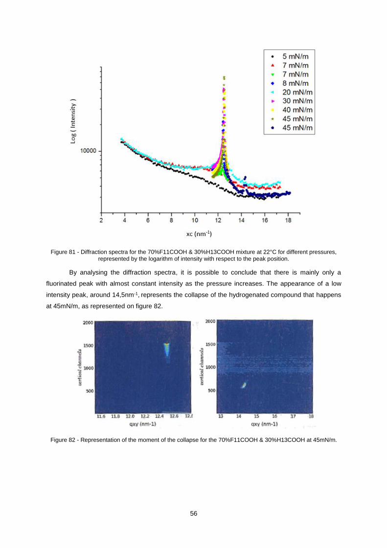
56


By analysing the diffraction spectra, it is possible to conclude that there is mainly only a

fluorinated peak with almost constant intensity as the pressure increases. The appearance of a low

intensity peak, around 14,5nm-1, represents the collapse of the hydrogenated compound that happens

at 45mN/m, as represented on figure 82.

Figure 82 - Representation of the moment of the collapse for the 70%F11COOH & 30%H13COOH at 45mN/m.

57

The variation of peak position and width with respect to the pressure is represented on figures

83 and 84.



Figure 84 - Width of the peak of 70%F11COOH & 30%H13COOH mixture with respect to the pressure at 22°C where the blue dots represent the fluorinated type molecules and the orange dot the hydrogenated.

By analysing the results on figure 83, there is a clear transition between the rich fluorinated

liquid and a fluorinated LC phase that has a constant value of xc around 12,5nm-1, which may also

indicate the presence of a crystal. Below 7,5mN/m the increase of pressure causes the position of the

peak to shift to higher values until it reaches the LC phase. The low width value can indicate the

presence of a crystal as the maximum width value for pressures higher than 7,5mN/m is 0,2nm-1.

Secondly, the results at 6°C are presented in the diffraction spectra on figure 85.


9,5

10

10,5

11

11,5

12

12,5

13

13,5

14

14,5

0 5 10 15 20 25 30 35 40 45 50

xc (

nm

-1)

P (mN/m)

0

0,5

1

1,5

2

2,5

3

3,5

4

4,5

0 5 10 15 20 25 30 35 40 45 50

w (

nm

-1)

P (mN/m)

58

From analysing the diffraction spectra, it is clear that the intensity of the peak is almost constant

with the increase of pressure, as well as the peak’s position. This is better visible on figure 86 where the

peak position is represented with respect to the pressure.



hydrogenated.


type molecules and the orange dot the hydrogenated.

A fluorinated rich LC phase is present for pressures higher than 5mN/m. The fluorinated

compound has a peak position around 12,5nm-1 and, since the width has low values, it is possible that

some fluorinated crystals were formed. The collapse of the hydrogenated molecules happens at

45mN/m and it’s represented by a single peak present at higher values of xc.

II.4.2.4 Phase Diagram

All the experiments performed to the mixtures had the final purpose of plotting a possible phase

diagram. To simplify the diagram, some small acronyms were used as detailed on table 10.

Table 10 - Acronyms used to simplify the understanding of the phase diagram.

Acronyms Meaning Acronyms Meaning

F Fluorinated LF Liquid Fluorinated

H Hydrogenated LH Liquid Hydrogenated

L Liquid LCF Liquid Condensed Fluorinated

G Gas LCH Liquid Condensed Hydrogenated

In the first place, the millimetric triangle was divided into intervals of pressure, on the right, and

intervals of percentage. The top of the triangle has a scale of percentage where all the four mixtures

analysed were correctly placed considering that the vertices corresponded to the pure compounds. The

four corresponding points and the third vertex were connected using a dashed line throughout which the

changes will be analysed as the pressure varies.

12

12,5

13

13,5

14

14,5

0 5 10 15 20 25 30 35 40 45 50

xc (

nm

-1)

P (mN/m)

0

0,05

0,1

0,15

0,2

0,25

0 5 10 15 20 25 30 35 40 45 50

w (

nm

-1)

P (mN/m)

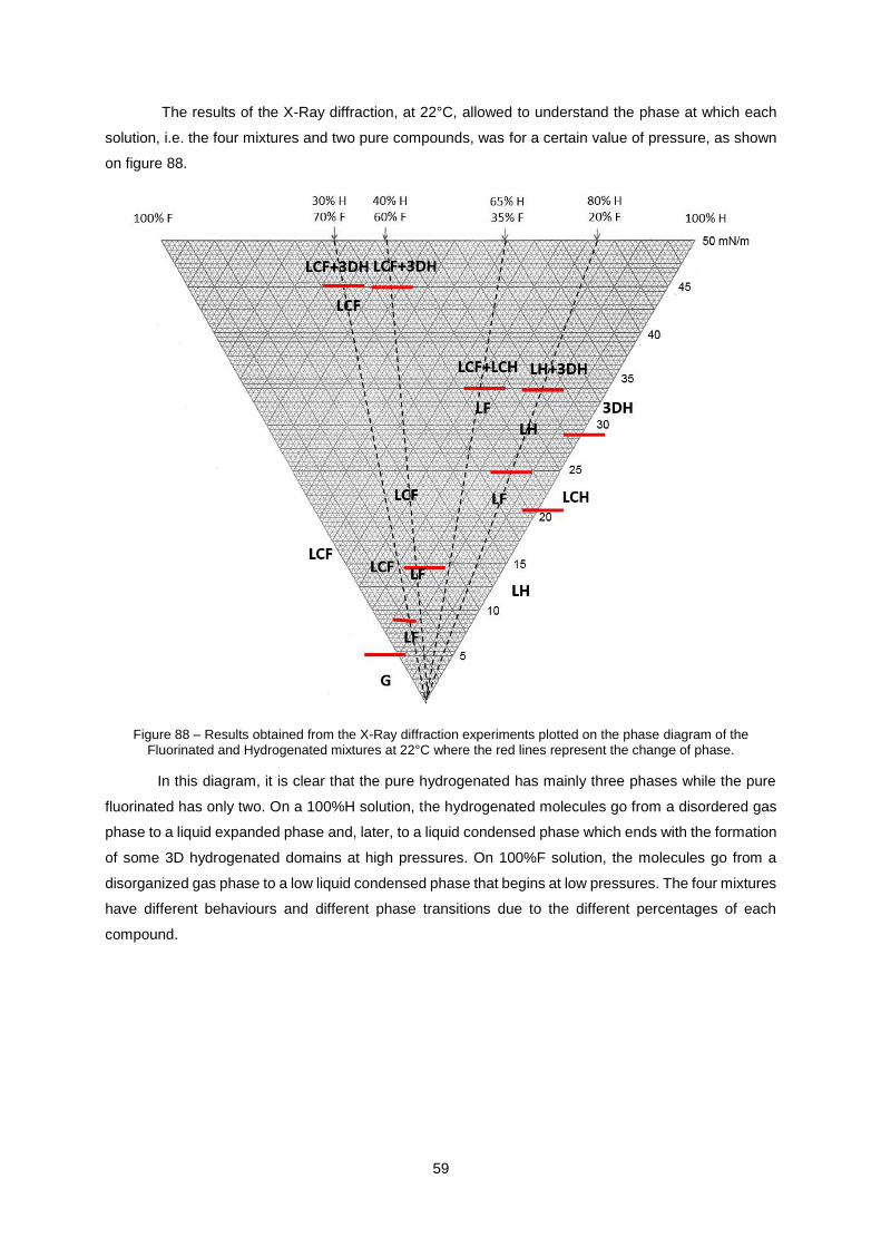
59

The results of the X-Ray diffraction, at 22°C, allowed to understand the phase at which each

solution, i.e. the four mixtures and two pure compounds, was for a certain value of pressure, as shown

on figure 88.

Figure 88 – Results obtained from the X-Ray diffraction experiments plotted on the phase diagram of the Fluorinated and Hydrogenated mixtures at 22°C where the red lines represent the change of phase.

In this diagram, it is clear that the pure hydrogenated has mainly three phases while the pure

fluorinated has only two. On a 100%H solution, the hydrogenated molecules go from a disordered gas

phase to a liquid expanded phase and, later, to a liquid condensed phase which ends with the formation

of some 3D hydrogenated domains at high pressures. On 100%F solution, the molecules go from a

disorganized gas phase to a low liquid condensed phase that begins at low pressures. The four mixtures

have different behaviours and different phase transitions due to the different percentages of each

compound.

60

Considering the phases represented on figure 88, it is possible to estimate the limits of the

different phase domains and create a complete phase diagram for the fluorinated and hydrogenated

mixtures at 22°C. The complete result is displayed on figure 89.

Figure 89 - Phase diagram of the fluorinated and hydrogenated mixture at 22°C where the dashed lines represent uncertain limits.

61

Considering some BAM images observed, it is uncertain if the gas phase is extinct in the range

presented on figure 89. Although the limits of the gas phase are not well defined, it is possible that, at

low values of pressure, the gas phase coexists with the other existing phases. The hypothetical limits of

this phase and the corresponding coexistences are represented on figure 90.

Figure 90 - Phase diagram of the fluorinated and hydrogenated mixture at 22°C with the inclusion of a broader gas phase, where the dashed lines represent uncertain limits.

62

For 6°C the same procedure was followed and the phase diagram obtained is presented on

figure 91. At this temperature, both pure compounds go from a gas phase directly to a liquid condensed

phase. The mixtures don’t present the same behaviour and, for high percentages of hydrogenated, there

is the existence of a LE phase. This translates into an appearance of a LE domain on the phase diagram.

Figure 91 - Phase diagram of the fluorinated and hydrogenated mixture at 6°C where the dashed line represents an uncertain limit.

63

Just like for 22°C, the limits of the gas phase are also unknown at low temperature. It is possible

that there are some coexistences between the gas phase and the LE and LC phases at low pressures.

Some hypothetical limits were considered to define this phase and its coexistences, as represented on

figure 92.

Figure 92 - Phase diagram of the fluorinated and hydrogenated mixture at 6°C with the inclusion of a broader gas phase, where the dashed lines represent uncertain limits.

64

II.5 F8H14

II.5.1 Isotherms

Some isotherms were recorded for the semi-fluorinated compound, F8H14, at different

temperatures as displayed on figure 93.

Figure 93 - Isotherms of F8H14 at 5°C, 15°C, 18°C and 20°C.

For values of molecular area higher than 0,35nm2/mol, there is a plateau at zero pressure that

represents the coexistence between the gas phase and the LC phase of the semi-fluorinated compound.

As referred before, the fluorinated chains are rigid and therefore the molecules go from a gas phase

directly into a LC phase. A lift-off around 0,33nm2/mol indicates the suppression of the gas phase and,

as the pressures rises, the domains are forcibly tighter packed until the collapse is reached at a certain

pressure between 6 and 9mN/m depending on the temperature.

A second plateau is visible between approximately 0,27nm2/mol and 0,07nm2/mol. This plateau

corresponds to the collapse of the monolayer and indicates that the film is no longer in a monolayer

state.

It is clear the influence of temperature in the behaviour of the isotherm. At low temperature, the

gas phase is suppressed at lower values of molecular area, which means that the film needs to be

further compressed in order to enter the LC phase and initiate the lift-off. This is represented by a slightly

shift of the isotherm to the left.

The influence of the temperature is also noticeable on the compressibility values of the film. It

is important to note that, at all the four temperatures analysed, there is a slight change of slope in the

first lift-off between 3mN/m and 5mN/m. This indicates the change from a first LC phase to a second LC

phase. Consequently, two different compressibility values of a LC phase can be calculated for every

isotherm as shown on table 11.

-1

4

9

14

19

24

0 0,05 0,1 0,15 0,2 0,25 0,3 0,35 0,4 0,45 0,5

P (

mN

/m)


20°C

18°C

15°C

5°C

65

Table 11 - Compressibility values of the F8H14 at 20°C, 18°C, 15°C and 5°C and the correspondent region between which the compressibility was calculated.

Compressibility

(m/N) Compressibility

(m/N)

Temperature (°C)

First LC phase Region (mN/m) Second LC phase

Region (mN/m)

20 20,45 1,1-4 13,3 4-8

18 13,05 1,2-5 7,09 5-7,7

15 12,76 0,7-3,5 8,23 4-6,7

5 14,11 1-5 7,92 5-8,6

The compressibility results don’t show any particular tendency but it is clear that, at 20°C, the

first LC phase has a much higher slope compared to the other isotherms which translates into a higher

compressibility value. It is also evident that the second LC phase has much lower compressibility values

than the first one. Apart from the results obtained for 20°C, the compressibility values of the other three

temperatures are rather similar which might indicate that the F8H14 compressibility is not mainly

affected by the temperature.

II.5.2 X-Ray Diffraction

The F8H14 was analyzed under the X-Ray diffraction technique. The results, at 18°C, are

displayed on figures 94 and 95 that represent the variation of peak position and width with pressure.

Figure 94 - Position of the peak of F8H14 with

respect to the pressure at 18°C.

Figure 95 - Width of the peak of F8H14 with respect

to the pressure at 18°C.

Since the monolayer collapses at low pressure, the X-Ray diffraction experiment was only

performed below 10mN/m. It is clear that the behaviour observed is the opposite of what was expected,

comparing to previous X-Ray diffraction results. Not only the peak shifts to lower values but also the

width increases with pressure. As the barriers compact the film and the pressure increases, it is

expected the decrease of the peak’s width which would lead to bigger domains being formed as the LC

phase initiates. Therefore, the X-Ray diffraction results obtained are not significant and were only

considered to evaluate if the value of peak’s position was around 12,5nm-1, as expected for a fluorinated

type molecule.

12,43

12,44

12,45

12,46

12,47

12,48

12,49

12,5

0 2 4 6 8

xc (

nm

-1)

P (mN/m)

0

0,2

0,4

0,6

0,8

1

1,2

1,4

1,6

0 2 4 6 8

w (

nm

-1)

P (mN/m)

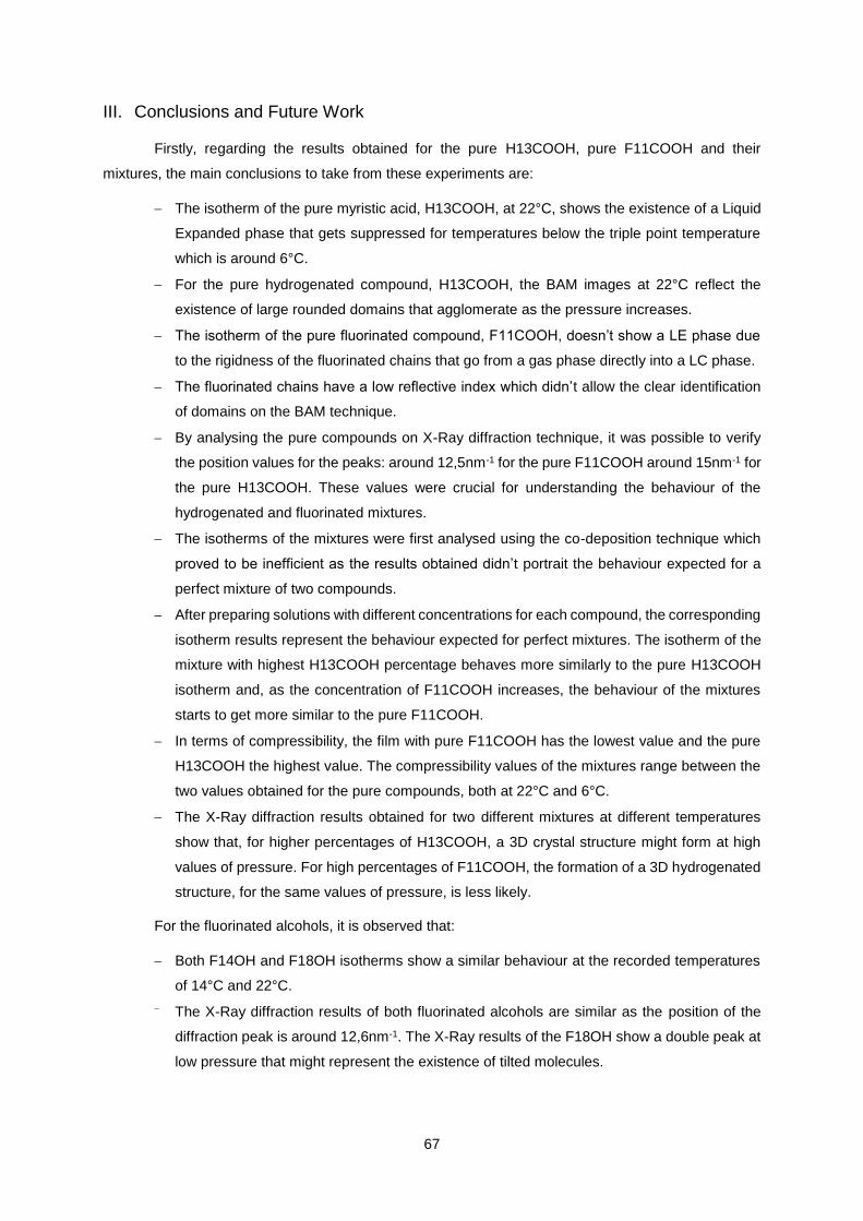
67

III. Conclusions and Future Work

Firstly, regarding the results obtained for the pure H13COOH, pure F11COOH and their

mixtures, the main conclusions to take from these experiments are:

The isotherm of the pure myristic acid, H13COOH, at 22°C, shows the existence of a Liquid

Expanded phase that gets suppressed for temperatures below the triple point temperature

which is around 6°C.

For the pure hydrogenated compound, H13COOH, the BAM images at 22°C reflect the

existence of large rounded domains that agglomerate as the pressure increases.

The isotherm of the pure fluorinated compound, F11COOH, doesn’t show a LE phase due

to the rigidness of the fluorinated chains that go from a gas phase directly into a LC phase.

The fluorinated chains have a low reflective index which didn’t allow the clear identification

of domains on the BAM technique.

By analysing the pure compounds on X-Ray diffraction technique, it was possible to verify

the position values for the peaks: around 12,5nm-1 for the pure F11COOH around 15nm-1 for

the pure H13COOH. These values were crucial for understanding the behaviour of the

hydrogenated and fluorinated mixtures.

The isotherms of the mixtures were first analysed using the co-deposition technique which

proved to be inefficient as the results obtained didn’t portrait the behaviour expected for a

perfect mixture of two compounds.

After preparing solutions with different concentrations for each compound, the corresponding

isotherm results represent the behaviour expected for perfect mixtures. The isotherm of the

mixture with highest H13COOH percentage behaves more similarly to the pure H13COOH

isotherm and, as the concentration of F11COOH increases, the behaviour of the mixtures

starts to get more similar to the pure F11COOH.

In terms of compressibility, the film with pure F11COOH has the lowest value and the pure

H13COOH the highest value. The compressibility values of the mixtures range between the

two values obtained for the pure compounds, both at 22°C and 6°C.

The X-Ray diffraction results obtained for two different mixtures at different temperatures

show that, for higher percentages of H13COOH, a 3D crystal structure might form at high

values of pressure. For high percentages of F11COOH, the formation of a 3D hydrogenated

structure, for the same values of pressure, is less likely.

For the fluorinated alcohols, it is observed that:

Both F14OH and F18OH isotherms show a similar behaviour at the recorded temperatures

of 14°C and 22°C.

The X-Ray diffraction results of both fluorinated alcohols are similar as the position of the

diffraction peak is around 12,6nm-1. The X-Ray results of the F18OH show a double peak at

low pressure that might represent the existence of tilted molecules.

68

For a mixture of F11COOH and F18OH there is complete segregation of both compounds

as demonstrated by the X-Ray diffraction results.

Lastly, for the semi fluorinated compound, F8H14:

It is clear the influence of the temperature in the behaviour of the isotherm, as it slightly shifts

to the right with temperature increase.

The collapse of the monolayer occurs at low pressure, below 10mN/m, and the film remains

stabilized during further compression until it collapses around 22mN/m at a possible double-

layer or tri-layer state.

In the future, it is important to continue the work developed in order to improve the knowledge

on this field and contribute to the scientific community so the fluorinated molecular films can be used for

more applications. For all the compounds analyzed it is important to perform Atomic Force Microscopy

to complement the isotherms and X-Ray diffraction results and to better understand the microscopic

behavior and properties of the surface.

69

IV. References

Akamatsu,S., Rondelez, F., Fluorescence microscopy evidence for two different LE-LC phases

transitions in Langmuir monolayers of fatty acids. HAL archives-ouvertes.fr, Jan 1991.

Als-Nielsen, J. and McMorrow, Des, Elements of Modern X-Ray Physics. John Wiley & Sons. 2001.

Averill, B. and Eldredge, P., General Chemistry: Principles, Patterns, and Applications, V.1.0. 2011.

Bardin, L., Faure, M.-C., Filipe, E., Fontaine, P. and Goldmann, M., Highly organized monolayer of a

semi-fluorinated alkane on a solid substrate obtained by spin-coating. Thin Solid Films, 2010.

Bardin, L., Faure, M.-C., Limagne, D., Chevallard, C., Konovalov, O., Filipe, E., Waton, G., Krafft, M.P.,

Goldmann, M. and Fontaine, P., Long-Range Nanometer-Scale Organization of Semifluorinated

Alkane Monolayers at the Air/Water Interface. Langmuir, 27, 13497-13505. 2011.

Barnes, P., Jacques S., Vickers, M., The Reciprocal Lattice. Birbeck College, University of London.

1997-2006. URL: http://pd.chem.ucl.ac.uk/pdnn/diff1/recip.htm (access date: May 2017)

Bhande, R. S., Landge, Y. A. and Giri, P. A., Study the Behavior of π-A Isotherm with Increasing Amount

of Octadecanoic acid at Air-Water Interface. Journal of Chemical and Pharmaceutical Research,

4(6): 3297-3301, 2012.

Celli, F., Nuclear Magnetic Resonance: A Dynamic View of Life. GotScience Magazine by Science

Connected. December 2015.

Ciatto, G., Chu, M. H., Fontaine, P., Aubert, N., Renevier, H. and Deschanvres, J. L., SIRIUS: A new

beamline for in situ X-Ray diffraction and spectroscopy studies of advanced materials and

nanostructures at the SOLEIL Synchrotron. Thin Solid Films, 617 (Part A): 48-54. 2016.

Costa, Ramalho M. and Andrade, C. R. Lourdes, Física do Estado Sólido. Departamento de Física

FCTUC. 2004.

Dinglasan-Panlilio, M.J.A, Mabury, S.A, Significant Residual Fluorinated Alcohols Present in Various

Fluorinated Materials, Environ. Sci. Technol., 40 (5), pp 1447-1453, 2006.

Fine, R. A., Millero, F. J., Compressibility of water as a function of temperature and pressure. Journal of

Chemical Physics, 59 (10): 5529-5536, 1973.

Fontaine, P., Ciatto, G., Aubert, N. and Goldmann M., Soft Interfaces and Resonant Investigation o

Undulator Source: A Surface X-Ray Scaterring Beamline to Study Organiz Molecular Films at

the SOLEIL Synchrotron. Science of Advanced Materials 6 (11), 2312-2316. 2014.

Fontaine, P., Bardin, L. Faure, M.-C., Filipe, E. and Goldmann, M., Evidence of lying molecules in the

structure of the most condensed phase of semi-fluorinated alkanes monolayers. 2017.

G.L. Gaines, Jr., Surface Activity of Semifluorinated alkanes: F(CF2)m(CH2)nH. Langmuir, 7, 3054 - 3056.

1991.

Hénon, S. and Meunier, Microscope at the Brewster Angle: Direct observation of first-order phase

transitions in monolayers. J. Rev. Sci. Instrum. 62, 936-939. 1991.

70

Hönig, D., Möbius, D., Direct visualization of monolayers at the air-water interface by Brewster angle

microscopy. J. Phys. Chem., 95, 4590-4592. 1991.

Huang, T. C., Predecki, P. K., Grazing-Incidence X-Ray Technique for Surface, Interface, and Thin-Film

Analysis. ICDD. URL: http://www.icdd.com/resources/axa/vol40/V40_056.pdf (access date:

September 2017).

Kaganer, V., Mohwald, H., Dutta, P., Structure and phase transitions in Langmuir monolayers. Rev.

Mod. Phys., Vol. 71, No. 3, 1999.

KSV NIMA, Brewster Angle Microscopes, Visualize your monolayer. Biolin Scientific Holding AB. 2016

URL: http://www.biolinscientific.com/ksvnima/products (access date: May 2017).

KSV NIMA, Langmuir and Langmuir-Blodgett Deposition Troughs. Biolin Scientific Holding AB. 2016.

URL: http://www.biolinscientific.com/ksvnima/technologies (access date: April 2017).

KSV NIMA AN 9, Imaging the Structure of thin films: Brewster Angle Microscopy. Biolin Scientific Holding

AB. 2016. URL: http://www.biolinscientific.com/application/ksv-nima-application-notes/ (access

date: May 2017).

Lin He, Feng Lin, Xingang Li, Hong Sui and Zhenghe Xu, Interfacial sciences in unconventional

petroleum production: from fundamentals to applications. Chem. Soc. Rev., Issue 15. 2015.

Mahan, Gerald, D., Crystal. Encyclopædia Britannica. April 22, 2016. URL:

www.britannica.com/science/crystal (access date: May 2017).

Marra, W. C., Eisenberger, P. and Cho, A. Y. J. Appl. Phys., 50, 6927, 1979.

Matsumoto, Y., Nakahara, H., Moroi, Y. and Shibata, O., Langmuir Monolayer Properties of

Perfluorinated Double Long-Chain Salts with Divalent Counterions of Separate Electric Charge

at the Air−Water Interface. Langmuir, 2007, Vol.23, No.19, pp 9629-9640.

NSRRC, Synchrotron Radiation – A Form of Light. National Synchrotron Radiation Research Center.

2010. URL: http://www.nsrrc.org.tw/english/lightsource.aspx (access date: September 2017).

Petrucci, R. H., Herring, F. G., Madura, J. D., Bissonnette, C., General Chemistry: Principles and Modern

Applications. Upper Saddle River, NJ : Prentice Hall, 2007.

Petty, M., Langmuir-Blodgett Films: An Introduction. Cambridge University Press, 1996.

Rontu, N., Vaida, V., Miscibility of Perfluorododecanoic Acid with Organic Acids at the Air-Water

Interface. J. Phys. Chem, 111, 9975-9980. 2007.

Sabín, J., Prieto, G., Estelrich, J., Sarmiento, F., Costas, M., Insertion of semifluorinated diblocks on

DMPC and DPPC liposomes. Influence on the gel and liquid states of the bilayer. Journal of

Colloid and Interface Science, 2010.

Stark, G., X-Ray Radiation Beam. Encyclopædia Britannica. July 3, 2017. URL:

https://www.britannica.com/science/X-ray (access date: September 2017).

71

Teixeira, M., Complex Interfacial Behavior of Mixtures of Fluorinated and Hydrogenated Alcohols.

Master Thesis, IST. 2014.

Viitala, T., Insoluble Monolayers: Preparation, Characterization and use in functional surfaces and

nanotechnology. KSV Instruments, 2006.

Vlassopoulos, D., Geue, T., Müllen, K., Berger, R. and Butt, H.-J., Structural and Viscoelastic Properties

of Semifluorinated Alkane Monolayers at the Air/Water Interface. 2013.

Wang, G.-C., Lu, T.-M., RHEED Transmission Mode and Pole Figures: Thin Film and Nanostructure

Texture Analysis. Springer Science + Business Media New York. 2014.

Warren, B. E., X-Ray Diffraction. Addison-Wesley Publishing Company, Inc., Reading MA/Dover,

Mineola NY. 1969.

Wood, E. A., Vocabulary of Surface Crystallography. Journal of Applied Physics, Volume 35, Number

4. April 1964.

1

V. Appendix

V.1 Stability Tests

A stability test consists in compressing the film until a value of pressure before the collapse. By

stopping the barriers and letting the film rest on the Langmuir trough for a certain amount of time, it is

possible to visualize if there is any change of area or pressure. Then, an expansion phase begins with

the goal of evaluating the reproducibility of the isotherm. If the compression isotherm is similar to the

one recorded during expansion, with minor shifts, the isotherm can be considered reproducible.

Figure A 1 - Stability test for the 60%F11COOH & 40%H13COOH at 6°C with a resting time of 30 minutes.

Figure A 2 - Stability test for the F8H14 at 15°C with a resting time of 15 minutes.

0

2

4

6

8

10

12

14

16

18

20

0,2 0,3 0,4 0,5 0,6 0,7 0,8 0,9 1

P (

mN

/m)


compression

expansion

-1

0

1

2

3

4

5

0,25 0,3 0,35 0,4 0,45 0,5

P (

mN

/m)


compression

expansion

2



0

1

2

3

4

5

0,25 0,3 0,35 0,4 0,45 0,5

P (

mN

/m)


compression

expansion

-1

0

1

2

3

4

5

0 0,05 0,1 0,15 0,2 0,25 0,3 0,35 0,4 0,45 0,5

P (

mN

/m)


compression

expansion

3

V.2 X-Ray Diffraction

V.2.1 H13COOH

Figure A 5 - Width of the diffraction peak of pure H13COOH with respect to the pressure at 6°C.

Figure A 6 - Area of the diffraction peak of pure H13COOH with respect to the pressure at 6°C.

V.2.2 F11COOH



Figure A 9 - Position of the (11) diffraction peak of pure

F11COOH with respect to the pressure at 6°C.

Figure A 10 - Position of the (20) diffraction peak of

pure F11COOH with respect to the pressure at 6°C.

0,05

0,25

0,45

0,65

0,85

1,05

0 5 10 15 20 25

w (

nm

-1)

P (mN/m)

200

700

1200

1700

2200

2700

3200

0 5 10 15 20 25

A n

m2 )

P (mN/m)

0

0,05

0,1

0,15

0,2

0,25

0 5 10 15 20 25 30 35

w (

nm

-1)

P (mN/m)

450

950

1450

1950

2450

2950

3450

3950

4450

0 5 10 15 20 25 30 35

A (

nm

2 )

P (mN/m)

21,5

21,52

21,54

21,56

21,58

21,6

21,62

21,64

21,66

0 5 10 15 20 25 30 35

xc (

nm

-1)

P (mN/m)

24,8

24,82

24,84

24,86

24,88

24,9

24,92

24,94

24,96

24,98

25

0 5 10 15 20 25 30 35

xc (

nm

-1)

P (mN/m)

4

Figure A 11 - Width of the (11) diffraction peak of pure








Figure A 16 - Area of the (10) diffraction peak of pure


0

0,01

0,02

0,03

0,04

0,05

0,06

0,07

0,08

0,09

0,1

0 5 10 15 20 25 30 35

w (

nm

-1)

P (mN/m)

0

0,01

0,02

0,03

0,04

0,05

0,06

0,07

0,08

0,09

0,1

0 5 10 15 20 25 30 35

w (

nm

-1)

P (mN/m)

100

105

110

115

120

125

0 5 10 15 20 25 30 35

A (

nm

2 )

P (mN/m)

80

85

90

95

100

105

110

115

120

0 5 10 15 20 25 30 35

A (

nm

2 )

P (mN/m)

0

0,02

0,04

0,06

0,08

0,1

0,12

0,14

0,16

0,18

0,2

0 5 10 15 20 25 30 35 40 45 50

w (

nm

-1)

P (mN/m)

0

100

200

300

400

500

600

700

800

0 5 10 15 20 25 30 35 40 45 50

A (

nm

2 )

P (mN/m)

5

V.2.3 F14OH

Figure A 17 - Width of the (10) diffraction peak of F14OH

with respect to the pressure at 22°C.

Figure A 18 - Area of the (10) diffraction peak of

F14OH with respect to the pressure at 22°C.

Figure A 19 - Position of the (11) diffraction peak of F14OH with respect to the pressure at 22°C.


Figure A 21 - Width of the (11) diffraction peak of F14OH with respect to the pressure at 22°C.

Figure A 22 - Width of the (20) diffraction peak of F14OH with respect to the pressure at 22°C.

0,015

0,017

0,019

0,021

0,023

0,025

0,027

0,029

0,031

0,033

0,035

0 10 20 30 40

w (

nm

-1)

P (mN/m)

60

160

260

360

460

560

660

760

860

960

1060

0 10 20 30 40

A (

nm

2 )

P (mN/m)

21,76

21,78

21,8

21,82

21,84

21,86

21,88

0 10 20 30 40

xc (

nm

-1)

P (mN/m)

25,12

25,14

25,16

25,18

25,2

25,22

25,24

25,26

25,28

0 10 20 30 40

xc (

nm

-1)

P (mN/m)

0,015

0,02

0,025

0,03

0,035

0,04

0,045

0,05

0,055

0,06

0 10 20 30 40

w (

nm

-1)

P (mN/m)

0,015

0,025

0,035

0,045

0,055

0,065

0,075

0,085

0 10 20 30 40

w (

nm

-1)

P (mN/m)

6

Figure A 23 - Area of the (11) diffraction peak of F14OH with respect to the pressure at 22°C.


V.2.4 F18OH

Figure A 25 - Width of the (10) diffraction peak of F18OH with respect to the pressure at 18°C, where the orange triangles represent the sum of the values of the double

peak.

Figure A 26 - Area of the (10) diffraction peak of F18OH with respect to the pressure at 18°C, where the orange triangles represent the sum of the values of the

double peak.



30

35

40

45

50

55

0 10 20 30 40

A (

nm

2 )

P (mN/m)

10

15

20

25

30

35

40

45

50

55

0 10 20 30 40

A (

nm

2 )

P (mN/m)

0

0,02

0,04

0,06

0,08

0,1

0,12

0 10 20 30 40

w (

nm

-1)

P (mN/m)

0

500

1000

1500

2000

2500

3000

0 10 20 30 40

A (

nm

2)

P (mN/m)

21,82

21,84

21,86

21,88

21,9

21,92

21,94

0 10 20 30 40

xc (

nm

-1)

P (mN/m)

25,21

25,22

25,23

25,24

25,25

25,26

25,27

25,28

25,29

25,3

0 10 20 30 40

xc (

nm

-1)

P (mN/m)

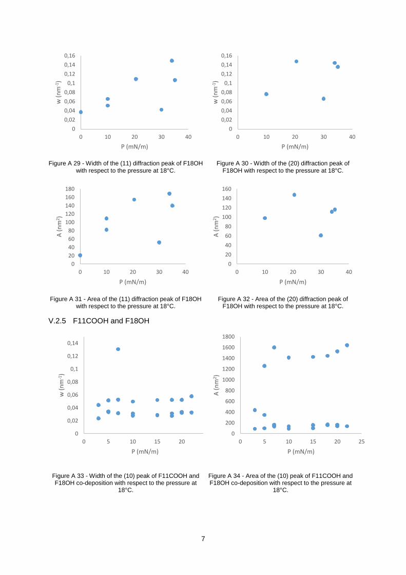
7

Figure A 29 - Width of the (11) diffraction peak of F18OH

with respect to the pressure at 18°C.

Figure A 30 - Width of the (20) diffraction peak of

F18OH with respect to the pressure at 18°C.



V.2.5 F11COOH and F18OH

Figure A 33 - Width of the (10) peak of F11COOH and F18OH co-deposition with respect to the pressure at

18°C.

Figure A 34 - Area of the (10) peak of F11COOH and F18OH co-deposition with respect to the pressure at

18°C.

0

0,02

0,04

0,06

0,08

0,1

0,12

0,14

0,16

0 10 20 30 40

w (

nm

-1)

P (mN/m)

0

0,02

0,04

0,06

0,08

0,1

0,12

0,14

0,16

0 10 20 30 40

w (

nm

-1)

P (mN/m)

0

20

40

60

80

100

120

140

160

180

0 10 20 30 40

A (

nm

2)

P (mN/m)

0

20

40

60

80

100

120

140

160

0 10 20 30 40

A (

nm

2)

P (mN/m)

0

0,02

0,04

0,06

0,08

0,1

0,12

0,14

0 5 10 15 20 25

w (

nm

-1)

P (mN/m)

0

200

400

600

800

1000

1200

1400

1600

1800

0 5 10 15 20 25

A (

nm

2 )

P (mN/m)

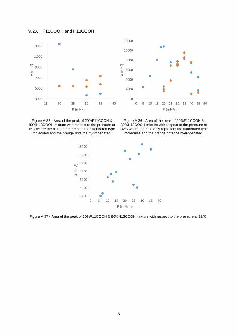
8

V.2.6 F11COOH and H13COOH

Figure A 35 - Area of the peak of 20%F11COOH & 80%H13COOH mixture with respect to the pressure at 6°C where the blue dots represent the fluorinated type




Figure A 37 - Area of the peak of 20%F11COOH & 80%H13COOH mixture with respect to the pressure at 22°C.

3000

5000

7000

9000

11000

13000

15 20 25 30 35 40

A (

nm

2)

P (mN/m)

0

2000

4000

6000

8000

10000

12000

0 5 10 15 20 25 30 35 40 45 50

A (

nm

2)

P (mN/m)

1200

3200

5200

7200

9200

11200

13200

0 5 10 15 20 25 30 35 40

A (

nm

2 )

P (mN/m)

9



Figure A 39 - Area of the peak of 35%F11COOH & 65%H13COOH mixture with respect to the pressure at 22°C where the blue dots represent the fluorinated




Figure A 41 - Area of the peak of 60%F11COOH & 40%H13COOH mixture with respect to the pressure at

22°C where the blue dots represent the fluorinated type molecules and the orange dot the hydrogenated.



Figure A 43 - Area of the peak of 70%F11COOH & 30%H13COOH mixture with respect to the pressure at

22°C where the blue dots represent the fluorinated type molecules and the orange dot the hydrogenated

70

570

1070

1570

2070

2570

3070

3570

4070

4570

5 10 15 20 25 30 35 40 45 50

A (

nm

2 )

P (mN/m)

170

2170

4170

6170

8170

10170

12170

14170

16170

18170

20170

5 10 15 20 25 30 35 40 45

A (

nm

2 )

P (mN/m)

0

500

1000

1500

2000

2500

3000

3500

4000

4500

0 5 10 15 20 25 30 35 40 45 50

A (

nm

2 )

P (mN/m)

300

1300

2300

3300

4300

5300

6300

7300

8300

9300

0 5 10 15 20 25 30 35 40 45 50

A (

nm

2 )

P (mN/m)

0

1000

2000

3000

4000

5000

6000

0 20 40 60

A (

nm

2 )

P (mN/m)

0

20000

40000

60000

80000

100000

120000

140000

0 5 10 15 20 25 30 35 40 45 50

A (

nm

2 )

P (mN/m)

10

VI. Notes

nanostructured fluorinated molecular films · hidrogenado, foi possível estimar um diagrama de...

Documents