nasa contractor report 189597 {d-jl - … · nasa contractor report 189597 {d-jl _'_j finite...
TRANSCRIPT
NASA CONTRACTOR REPORT 189597 {D-Jl _'_J
FINITE ELEMENT ANALYSIS
OF THE STIFFNESS OF FABRIC
REINFORCED COMPOSITES
R. L. Foye
Lockheed Engineering and Sciences CompanyHampton, VA 23666
Contract NASI-19000
February 1992
National Aeronautics and
Space Administration
LANGLEY RESEARCH CENTER
Hampton, Virginia 23665-5225
(NASA-CR-189597) FINIIE ELEMENT ANALYSIS OF
[HE STIFFNESS OF FABRIC _EINFORCEO
COMPOSITES (Lockheed Engineering and
Sciences Corp.) 137 p CSCt ]tOG3124
N92-23102
Unclas
0085176
https://ntrs.nasa.gov/search.jsp?R=19920013859 2018-08-18T16:26:31+00:00Z
TABLE OF CONTENTS
SECTIONPAGE
i •
2.
3.
4.
.
,
7,
8.
LIST OF SYMBOLS
ABSTRACT
INTRODUCTION
REINFORCING GEOMETRY
HISTORICAL DEVELOPMENT
FABRIC ANALYSIS
4.1 Determination of Overall Elastic Constants
4.2 Unit Cell Boundary Conditions
4.3 Symmetry Boundary Conditions
SUBELEMENT MECHANICS
5.1Subcell Analysis
5.2 Subcell Transformation
ASSEMBLY AND SOLUTION
6.1 Discrete Unit Cell Boundary Conditions
6.2 Discrete Symmetry Boundary Conditions
6.3 General Statement of the Discrete Problem
COMPUTER PROGRAM DESCRIPTION
SIMPLE APPLICATIONS
8.1 Fiber Path Variation
8.2 Void Analysis
iii
v
i
4
6
8
8
i0
12
14
15
19
22
22
23
24
27
29
3O
31
9.
10.
SECTION
WOVEN FABRIC APPLICATIONS
9.1 Realistic Plain Weave Model
9,2 Other Weaves
BRAIDED FABRIC APPLICATIONS
i0.I Triaxial Braids
KNITTED FABRIC APPLICATIONS
CONCLUDING REMARKS
LIST OF REFERENCES
TABLES
FIGURES
APPENDIX I - PROGRAM LISTING
APPENDIX II INPUT DATA FORMAT
APPENDIX III - SAMPLE PROBLEM
PAGE
35
40
44
45
48
50
53
55
63
98
119
124
i i.
LIST OF SYMBOLS
a, b, c
A, B, C,
[B]
CW, CCW
D, [D], D..13
d (vol)
E,E..13
Ep
{F}
Gr
G,G.13
[HI, [J]
[k], [K]
NX, NY, NZ
psi, msi
s, IS],s..13
T
N.A.
U,V,W, Ui,Vi,W i
x,y,z,x,y,z
X, Y, Z, Xi,Y i, Z i
_' _' _ij" 7ij
{61g,
13 13
rlij, k
V, Vij
(_' _" _ij' _ij
1;, "_, Iij, 'l;ij
_), _).1
O, *i
2-D
3-D
Subcell side lengths
Unit cell side lengths
Strain/displacement matrix
Clockwise, counterclockwise
Stress-strain stiffness coefficients
Increment of volume
Young's modulus
Epoxy
Force vector
Graphite
Shear modulus
Coefficient matrix
Stiffness matrix
Number of node points on coordinate axes
6Pounds/square inch, 10 pounds/square inch
Stress-strain flexibility matrix
Matrix transpose
Not available/not applicable
Displacements in coordinate directions
Rectangular coordinates
Forces in coordinate directions
Shear strain
Displacement vector
Normal strain
Coefficients of mutual influence
Poisson's ratio
Normal stress
Shear stress
Volume fraction
Fiber orientation angle
Two dimensional
Three dimensional
iii

ABSTRACT
This report concerns the prediction of elastic moduli for fabric reinforced
composites. Many analysis methods previously applied to this problem are not
general enough for use with the more complex reinforcing geometries that have
been suggested for suppressing impact damage and general delamination. The
proposed analysis places no restrictions on fabric microgeometry except that
it be determinate within some repeating rectangular pattern. No assumptions
are made regarding fiber cross-sectional shapes or fiber paths.
The analysis is based on a mechanical model that consists of a single
rectangular unit cell which typically contains one repeating pattern of the
fabric design. Every unit cell is assumed to be surrounded on six sides by
identical unit cells, similarly oriented, with all common surfaces perfectly
bonded. Elastic analysis of one such cell element yields all 3-D moduli of
the composite.
For analysis purposes the unit cell is assumed to be divisible into small
rectangular subcells in which the reinforcing geometries are easier to
visualize, define, and analyze. Details of micromodeling and the use of
single, finite element hexahedra to mathematically represent each subcell are
described in this report. The analysis is applied to a variety of woven,
braided, and knitted fabric reinforcements in epoxy matrix. A special purpose
computer program based on this analysis is also described. Moduli predictions
from this program are compared to fabric reinforced composite test data. A
program listing with sample input and output is included in the Appendices.
V
PRECEDJI_iG PAGE BLANK NOT FILMED
i. INTRODUCTION
Complex fibrous preforms (made from weaves, braids, knits, XYZ construction, etc.)
are under consideration for use as composite reinforcing materials. As
reinforcers, these preforms should increase impact resistance, reduce lay up time,
and generally improve interlaminar properties. Use of these textile structures
introduces a variety of both new and old manufacturing processes into the
fabrication cycle and creates an intermediate material stage. This stage consists
of an array of systematically interlaced fiber bundles (yarns or tows) surrounded
and impregnated by a matrix material. The basic repeating structural element in
this array has characteristic dimensions that are much larger than a single fiber
diameter, but are on the order of the structural plate or shell wall thickness
(Figure i) . From an analyst's point of view this stage creates a gap between
micro-mechanics and laminate analysis, and requires a new level of mechanics
analysis. The term "fabric mechanics" seems appropriate for categorizing this
level of composite mechanics. However, use of this terminology may confuse
textile engineers who normally associate fabric mechanics with unimpregnated
fabric behavior. The goals of fabric mechanics is to predict material properties
at the fabric reinforced composite level from knowledge of unidirectional
composite and bulk matrix material properties. This level of analysis is
necessary to reduce dependence on testing and to assist in data extrapolation and
interpretation. The influence of factors such as fiber curvature, misalignment,
and ply nesting are not conveniently assessed by either micro-mechanics or
laminate analysis. Fabric mechanics' role in the scheme of composite mechanics is
shown in Figure i. For laminates made from unidirectional material, fabric
mechanics is not required because micro-mechanics provides all the necessary
information for laminate analysis.
Although methods of fabric analysis are not firmly established, its goals are
identical to those of all mechanics analyses; namely, to predict stresses and
deformations within a deterministic structure as a result of prescribed external
loads or deformations. From these predictions (plus suitable failure criteria)
composite static properties of stiffness and strength can be estimated. The
limited objective of this report is to develop adequate capability (and a computer
code) to predict static stiffness of various fabric reinforced composites proposed
for minimizing impact damage. Several methods for predicting these properties
have been proposed, but they are built on many assumptions, and do not enjoy
widespread use or confidence.
The principal barrier to improved analyses is the geometric complexity of most
fabric microstructures. The proposed analysis crosses this barrier via two stages
of mechanical modeling. For example, consider the rib weave fabric microstructure
shown in Figure 2. This fabric geometry can be subdivided into small block
substructures or subcells (as shown in the same Figure). Simpler reinforcing
fiber geometry within each different subcell can be modeled by finite element
hexahedra. After reassembling the subcells the boundary conditions required to
simulate the six independent unit strain cases of 3-D elasticity may be enforced
(as in micro-mechanics). The resulting elastic solutions yield all necessary
information for computation of the 6 X 6 stiffness or flexibility matrix of the
composite. The approach is well-suited to computer analysis. A special propose
code has been written that predicts the stiffness of fabric reinforced composites
on the foregoing basis. A laminate analysis must be performed if several
different fabrics are combined into a thick, laminated structure. This approach
has the added advantage of lying within the range of experience of most structural
analysts.
2

One of the long range objectives of this work is to develop the capability of
estimating all of the 3-D static material property inputs required of transient
dynamic impact codes that analyze the response of composite target plates to
spherical impactors (Ref. i). This capability will permit rational selection of
woven, braided, and stitched fabric parameters to best meet impact damage
requirements with the least penalty to the basic static design properties.
2, REINFORCING GEOMETRY
In the textile sense, the term "fabric" is applicable to any network of bonded or
unbonded fibers which results in an essentially planar structure that is flexible
yet cohesive beyond the point of being self-supporting. The fabrics can be
categorized as having either a random distribution of fiber (as in a felt or
bonded flock) or an orderly distribution (as in weaves, braids or knits). Hybrids
of both are possible and some elements of order and disorder are always present in
both. Yarns or tows can also be continuous or discontinuous or a hybrid of both
(as in cut pile carpetS).
arranged in identifiable
considered. It is also
In this report, only fabrics made from continuous tows
and repetitious patterns of entanglement will be
assumed that this repetitious pattern has finite
dimensions and can be contained exclusively within the volume of a rectangular
prism. This prism is termed a "unit cell" of the fabric. Reproduction of this
unit cell, rigid transformation of it, and attachment to compatible surfaces of
other unit cells, allows any large planar area to be covered by this fabric, with
areal contours closely approximated by outer boundaries of units cells. Also unit
cells can by layered to fill any closed volume, even where minimum dimensions of
that volume are several orders of magnitude larger than unit cell dimensions. It
is assumed in this process that all common boundaries between unit cells are
perfectly bonded to each other.
This 3-D unit cell often visually relates to the 2-D fabric design plan that,
along with the harness draft and the chain draft, is typically used to describe a
weave pattern and to set up a shuttle loom to make that weave. The design plan is
a coded representation of a weave, whereas the unit cell is a true scale model of
the weave, albeit a somewhat idealized one. A design plan is usually drawn on 8 X
8 design paper. Columns represent warp yarns; rows represent fill yarns. Each
small square represents an intersection of one warp and one fill yarn. A shaded
square indicates that the fill yarn crosses over the warp yarn at that
intersection.
One unit cell representation of a plain weave is shown in Figure 3A. The
corresponding fabric design plan is shown in Figure 3B. But, neither the unit
cell nor the design plan are unique. Another very different unit cell of the same
weave is shown in Figure 3C.
Since unit cells are not unique, the question arises as to which unit cell should
form the basis for fabric analysis. The answer is that unit cell which is
simplest to analyze. Often, the simplest cell is presumed to be the smallest
cell. However, the smallest unit cell is frequently difficult to analyze,
particularly when it has complex boundaries, for example the twill weave (Figure
4). Boundaries of the smallest twill weave unit cell do not form a rectangular
prism. Hence, mechanical analysis of this weave can be difficult. The larger
unit cell of Figure 4C does not pose this problem.
Several rectangular unit cells for common weaves, knits and braids are shown in
Figure 5. For some complex fabrics, it is difficult to identify a rectangular
unit cell. For woven fabrics, one repeat of the design plan often resembles an
out-of-scale projection of a unit cell surface. But with knits or braids there is
no corresponding 2-D design plan. However, rectangular unit cells generally can
be established, although some liberties with the tow geometry may be required.
For example, some tow geometries like satin weaves (with large, complex,
rectangular, unit cells) contain smaller, simpler, trapezoidal, unit cells.
Slightly distorting the boundary of the smaller unit cell can make it rectangular
but this process entails some violation of the true microgeometry.
3. HISTORICAL DEVELOPMENT
Woven fiberglass cloth was the first reinforcing material with enough strength and
stiffness for general use on aircraft structures. However, relatively few fabric
weave styles saw extensive application. These fabrics were experimentally
characterized using epoxy and polyester resins and were treated like new
orthotropic materials with little consideration of fabric microstructural
analysis. Although it was known at that time that fabric microgeometry had a
significant effect on moduli and was one of the determining factors in stress
failure of this material, a convincing mechanical analysis of this problem was
beyond computational capabilities. The advent of filament winding and
unidirectional prepregging, along with increased capability in computing, soon
made such an analysis possible at the unidirectional level. It was assumed that a
wide range of fiber volume fractions and fiber cross-sectional shapes would
necessitate some type of micro-mechanics design/analysis cycle. Instead
unidirectional materials became even more standardized than fabrics. Test data
replaced micro-mechanics.
The search for improved impact resistance has brought about a renewal of interest
in more complex reinforcing geometries. Meanwhile, computing capability has kept
pace with materials development. This increased computing capability now allows
design and analysis of fabrics at a level comparable to design and analysis of
unidirectional materials. The number of geometric variables present and the
requirements of impact resistance suggest fabric reinforcements will play a role
in developing impact resistant composites.
First attempts to extend composite mechanics beyond the realm of planar analysis
arose in conjunction with carbon-carbon development for reentry vehicles (Ref 2).
These attempts ranged from 3-D versions of the rules of mixture and netting
analysis to finite element solutions. Fiber curvature was seldom considered.
Two-dimensional analysis of wavy fiber reinforced composites was considered by
some to be an initial step toward the analysis of true fabric reinforced
composites (Ref. 3). In this approach a single wavy fiber is treated as a curved
beam on an elastic foundation.
Another step toward geometric reality (Ref. 4) involved modeling of orthogonal
fiber arrays. However, the problem was reduced to two dimensions and solved by
finite elements.
Among the first to treat fabric mechanics as a true 3-D problem were Ishikawa,
Chou, et al., (Refs. 5 through ii). Based on assumed fiber paths and cross-
sectional shapes these authors developed a variety of models based largely on
"strength of materials" type idealizations and extended some of this work into the
nonlinear property realm.
Materials Sciences Corporation ......... a simple fabric model based on earlier
work on random fiber reinforcements (Ref. 12).
Another more refined approach was the attempt to fit fabric mechanics directly
into the context of laminated plate theory (Ref. 13). This analysis also
occasionally relies on "strength of materials" assumptions (Ref. 14).
The primary legacy of the previous work lies not in analytical details, but in the
modeling of complex fabric microgeometry with unit cells and subcells. Not only
does this reduce the geometry problem to smaller, "more digestible" pieces; it
also meshes with the finite element scheme of reducing a complex structure to an
assemblage of simpler ones which can be characterized, reassembled, and
manipulated to predict the response of the unit cell and the composite.

4. FABRIC ANALYSIS
For convenience in establishing thickness direction properties, each fabric
reinforced composite ply hereafter will be considered to be imbedded in a thick
laminate of identical plies layered such that each unit cell in each ply
represents one level in a vertical stacking of unit cells extending through the
full _hickness of the laminate (like stories in a multi-story building). For
example, treat each unit cell as a single brick in a stack bond wall (Figure 6).
A wide variety of other stacking arrangements are equally valid and can be
observed in laminates. Cursory investigations show these stacking variations to
be of secondary importance to the principal ply stiffness. A more thorough
investigation would be appropriate to strength analysis but of lower priority to
this study.
4.1 Determination of Overall Elastic Constants
Now consider a large cube of fabric reinforced composite material in which
dimensions of the cube are orders of magnitude greater than dimensions of the unit
cell. For most engineering purposes such a composite material can be considered
homogeneous and anisotropic with a linear stress-strain law of the form:
zz
- 1
_yz
_xz
_xy
m
S11 $12 $13 S14 S15 S16
$21 $22 $23 $24 $25 $26
S31 S32 S33 S34 S35 S36
$41 S42 $43 S44 S45 $46
S51 S52 S53 S54 S55 S56
S61 S62 S63 S64 S65 S66
(_xx
w
(_yy
(_zz
yz
xz
xy
(4.1)
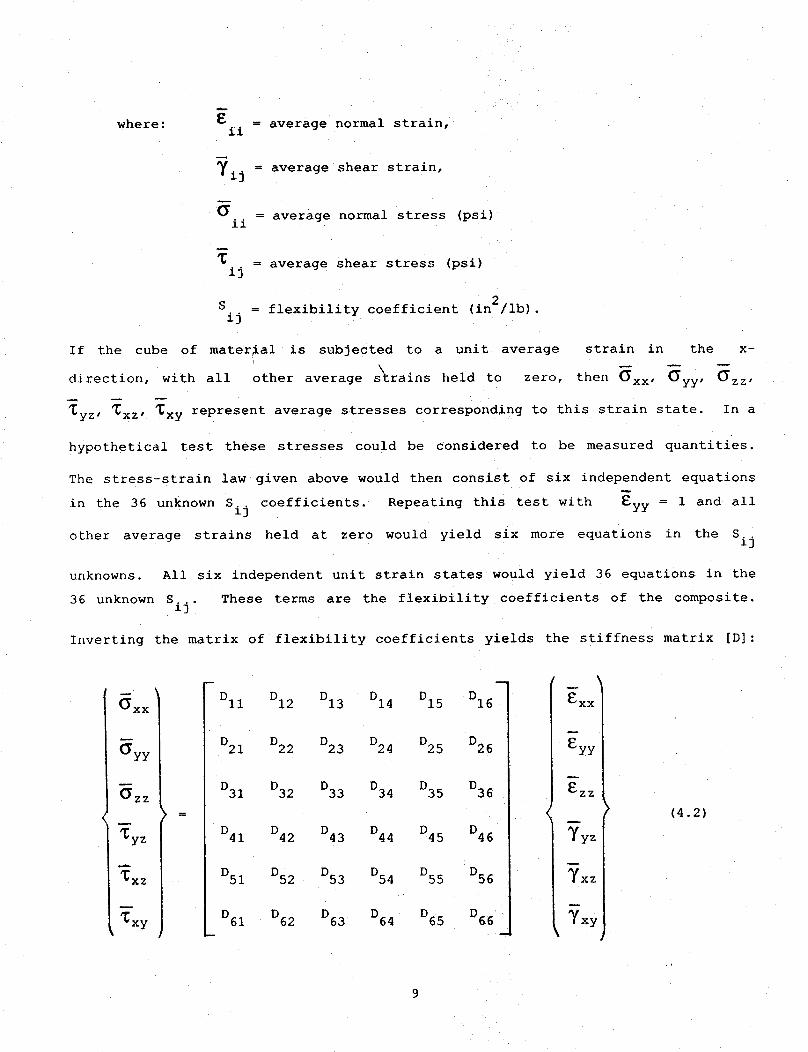
where: Eii = average normal strain,
_ij = average shear strain,
u
(_ = average normal stress (psi)ii
m
ij = average shear stress (psi)
= flexibility coefficient (in2/ib).S
ij
If the cube of material is subjected to a unit average strain in the x-
direction, with all other average s_rains held to zero, then _xx, _yy, _zz,
_yz, _xz, _xy represent average stresses corresponding to this strain state. In a
hypothetical test these stresses could be considered to be measured quantities.
The stress-strain law given above would then consist of six independent equations
in the 36 unknown Sij coefficients. Repeating this test with _yy = 1 and all
other average strains held at zero would yield six more equations in the S..13
unknowns. All six independent unit strain states would yield 36 equations in the
36 unknown S... These terms are the flexibility coefficients of the composite.13
Inverting the matrix of flexibility coefficients yields the stiffness matrix [D]:
(_xx
(_yy
(_zz
_yz
_xz
_xy
DII DI2 DI3 DI4 DI5 DI6
D21 D22 D23 D24 D25 D26
D31 D32 D33 D34 D35 D36
D41 D42 D43 D44 D45 D46
D51 D52 D53 D54 D55 D56
D61 D62 D63 D64 D65 D66
_xx
Eyy
_zz
_yz
m
_xz
Yxy
(4.2)

where: D.. = stiffness coefficient of composite (psi).13
E.,11 Vij, G..13 etc. for the composite can be obtained by considering the material
response to single nonzero components of each of the six average stresses
where: E = modulus of elasticity of material (psi),ii
V. = Poisson's Ratio,13
G.. = modulus of rigidity of material (psi).13
4.2 Unit Cell Boundary Conditions
Now return to the initial problem of obtaining the average composite stress
components _xx, _yy, _zz, _yz, _xz, _xy resulting from the average strain state
_ _ _ -=i _ = £ = 7xyxx " yy zz xz = = 0. (4.3)
This problem can be resolved by considering a single unit cell of the material,
sufficiently far removed from the surfaces to be free from edge, corner, or
surface effects. Since all such unit cells in the material are indistinguishable
from one another the response of any two unit cells to any uniform average stress
or strain state must be similar, except for rigid body motion.
Relative displacement of the eight corners of the unit cell are shown in Figure 7.
Any other set of relative displacements would be incompatible, inhomogeneous (in
the average strain sense), or in violation of the unit strain case that it
represents.
Now consider boundary conditions on surfaces of the unit cell. First consider
interlamina upper and lower surfaces of the cell. For every point on the upper
surface there is a corresponding point directly below it on the bottom surface
(Figure 8). Call these two points "image points" because the top image point on
I0
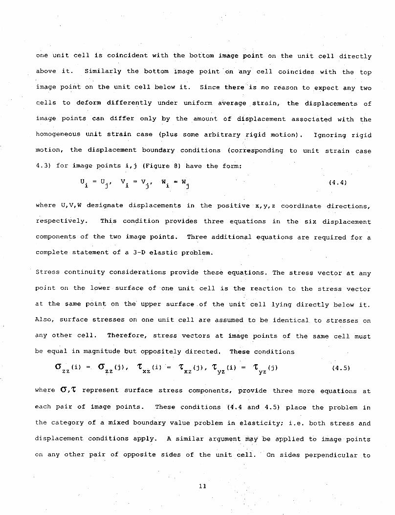
one unit cell is coincident with the bottom image point on the unit cell directly
above it. Similarly the bottom image point on any cell coincides with the top
image point on the unit cell below it. Since there is no reason to expect any two
cells to deform differently under uniform average strain, the displacements of
image points can differ only by the amount of displacement associated with the
homogeneousunit strain case (plus some arbitrary rigid motion). Ignoring rigid
motion, the displacement boundary conditions (corresponding to unit strain case
4.3) for image points i,j (Figure 8) have the form:
U. = U., V = V., W. = W. (4.4)z 3 z 3 z 3
where U,V,W designate displacements in the positive x,y,z coordinate directions,
respectively. This condition provides three equations in the six displacement
components of the two image points. Three additional equations are required for a
complete statement of a 3-D elastic problem.
Stress continuity considerations provide these equations. The stress vector at any
point on the lower surface of one unit cell is the reaction to the stress vector
at the same point on the upper surface of the unit cell lying directly below it.
Also, surface stresses on one unit cell are assumed to be identical to stresses on
any other cell. Therefore, stress vectors at image points of the same cell must
be equal zn magnitude but oppositely directed.
(_ (i) = (_ (j), • (i) = _ (j),zz zz xz xz yz
These conditions
(i) = _ (j)yz
(4.5)
where (_,_ represent surface stress components, provide three more equations at
each pair of image points. These conditions (4.4 and 4.5) place the problem in
the category of a mixed boundary value problem in elasticity; i.e. both stress and
displacement conditions apply. A similar argument may be applied to image points
on any other pair of opposite sides of the unit cell. On sides perpendicular to
11
the x-axis the U displacement condition has the more general form U. = U. + A,x 3
where A is a constant that accounts for the stretching in the x-direction.
Similar conditions can be specified for the other two normal strain cases.
Boundary conditions for the three unit shear strain cases differ from normal
strain cases only in that the constant terms that appear in some of the
displacement boundary conditions are associated with displacement components that
are parallel rather than normal to sides of the unit cell where they apply.
4.3 Symmetry Boundary Conditions
Structural symmetry often can be used to reduce the portion of the unit cell that
needs to be analyzed. However, boundary conditions on the plane of symmetry, and
the cell face parallel to the plane of symmetry, will differ from those conditions
previously stated. Consider only the special case where two parallel faces of the
reduced unit cell are both planes of symmetry.
First consider the three unit normal strain problems. All eight corners of the
reduced (by symmetry) unit cell now lie on planes of structural (and loading)
symmetry, but their pure displacement boundary conditions are not changed from the
previous discussion; i.e. their displacements are what establish the particular
unit strain case under consideration. Points lying on one plane of symmetry have
the traditional symmetry conditions of zero (or constant) normal displacement and
zero shear stress. Thus, stresses and displacements at image points that lie on
parallel planes of symmetry are no longer related through their boundary condition
equations.
12

Unit shear strain load cases divide into two categories: symmetric loading
categories and antisymmetric ones. Symmetric loading cases do not differ from
unit normal strain cases. Antisymmetric loading categories have boundary
conditions that are the converse of the symmetric ones; i.e., displacements
parallel to a plane of structural symmetry are zero (or constant), and stresses
normal to that plane are zero.
13
5. SUBELEMENT MECHANICS
The previous section (4.) of this report describes the elastic structure (the unit
cell), the various load (or displacement) cases applied to that structure, and the
boundary conditions prevailing on surfaces of the structure. This section
considers a numerical method for estimating internal (and surface) displacements
of the unit cell for each set of loads and boundary conditions. This analysis is
a direct application of the finite element method in which the unit cell
structure is idealized into a number of smaller polyhedra (subcells) joined
together at common vertices. The presumption is that stress, strain, and
displacement fields are simpler to approximate within the subcell, than in the
larger structure. Each subcell is then analyzed for the most general set of loads
(or displacements) at each of the vertices and reassembled into the unit cell
structure.
If the unit cell is in the shape of a rectangular prism it is convenient to
consider only subdivisions of the unit cell into smaller rectangular prisms
(subcells). The advantage of this restriction is that it simplifies the geometry
and the analysis, and eases coding for digital computation. This restriction is
one of convenience and is not particularly restrictive because fabric
microgeometries are often rectangular to some degree. For example, consider the
plain weave unit cell of Figure 9.* This unit cell of Figure 9 can be subdivided
into 16 subcells as shown. These subcells are all rectangular prisms, like the
unit cell.
* A subsequent section contains photomicrographs of aclual fabric reinforced composites, including a plain weave. The
sirrularities between cross sections of the more realistic c_it ceils which model the composite microstructure and the
pl-_tomicrographs are apparent.
14
If the warp and fill tows are similar and their paths are the same, then the 16
subcells are all simple transformations of each other; i.e., any one of their
reinforcing microgeometries can be reproduced by a combination of rigid motions
and reflections about the face planes of any one of the subcells. The
transformation makes the chore of describing microgeometry much simpler since a
detailed description of one subcell (mastercell) and a set of instructions for the
series of coordinate transformations will suffice to reconstruct the unit cell.
As another example consider the unit cell of the 2/2 rib weave construction with
similar warp and fill yarn geometries (Figure 2). This unit cell can be
constructed from a sequence of transformations of two master subcells designated I
and II in Figure 2.
5.1Subcell Analysis
Now consider the elastic analysis of a single rectangular subcell. For
incorporation into a finite element analysis at the simplest level, it is
necessary first to obtain a stiffness matrix relating the three components of
force, acting at each corner of the subcell, to the three components of
displacement at each corner. The method of obtaining this matrix is the central
problem in fabric reinforced composite stiffness analysis. Many possible
approaches exist. Simpler approaches often overlook fiber reinforcing detail.
Refined analyses lead to greater computational efforts than the problem warrants.
Hence, a compromise is needed. One compromise is suggested by the general energy
formulation for the stiffness matrix of rectangular finite element hexahedra (Ref.
15); l.e.,
15
[k] =vJ/J[B]T[D]fff [B] d(vol) (5.1)
where: [D] = 3-D material stiffness matrix,
[B] = strain/displacement matrix,
vol = volume
[D] contains only local material property distribution functions and [B] contains
only derivatives of displacement mode shapes. Superscript T designates matrix
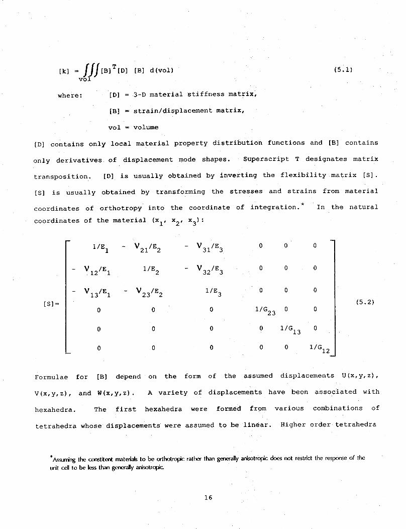
transposition. [D] is usually obtained by inverting the flexibility matrix [S].
[S] is usually obtained by transforming the stresses and strains from material
coordinates of orthotropy into the coordinate of integration. In the natural
coordinates of the material (x
[S] =
i' x2' x3) :
1/E 1 - V21/E 2 - V31/E 3 0 0
- VI2/E 1 I/E 2 - V32/E 3 0 0
- VI3/E 1 - V23/E 2 I/E 3 0 0
0 0 0 I/G23 0
0 0 0 0 I/G
0 0 0 0 0
13
I/G12
0
0
0
(5.2)
0
0
Formulae for [B] depend on the form of the assumed displacements U(x,y,z),
V(x,y,z), and W(x,y,z). A variety of displacements have been associated with
hexahedra. The first hexahedra were formed from various combinations of
tetrahedra whose displacements were assumed to be linear. Higher order tetrahedra
*Assuming the constitent materials to be orthotropic rather than generally anisotropic does not restrict the response of the
unit cell to be less than generally anisotropic_
16
were also used.
32 nodes.
were also
hexahedra.
Later, isoparametric families of hexahedra were used with 8, 20,
All nodes were located on element edges. Elements with internal nodes
investigated. Also used were super-elements formed from smaller
Displacement derivatives were used as nodal degrees of freedom also.
The intent of this study was to begin with simple elements, increasing their
complexity only as required to obtain acceptable accuracy for moduli predictions.
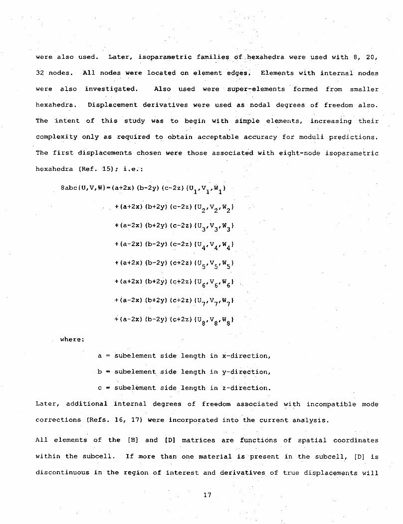
The first displacements chosen were those associated with eight-node isoparametric
hexahedra (Ref. 15); i.e. :
8abc{U,V,W}=(a+2x) (b-2y) (c-2z) {UI,VI,W I}
+ (a+2x) (b+2y) (c-2z) {U2,V2,W 2}
+ (a-2x) (b+2y) (c-2z) |U3,V3,W 3}
+ (a-2x) (b-2y) (c-2z) {U4,V4,W 4 }
+(a+2x) (b-2y) (c+2z){U5,V5,W 5}
+ (a+2x) (b+2y) (c+2z) {U6,V6,W 6}
+(a-2x) (b+2y) (c+2z) {U7,V7,W 7}
where:
+(a-2x) (b-2y) (c+2z){U8,V8,W 8}
a = subelement side length in x-direction,
b = subelement side length in y-direction,
c = subelement side length in z-direction.
Later, additional internal degrees of freedom associated with incompatible mode
corrections (Refs. 16, 17) were incorporated into the current analysis.
All elements of the [B] and [D] matrices are functions of spatial coordinates
within the subcell, if more than one material is present in the subcell, [D] is
discontinuous in the region of interest and derivatives of true displacements will
17

also be discontinuous. Nevertheless, the integration for obtaining the stiffness
matrix can still be performed. Mathematically, functions of class C {withoutf O
continuous first derivatives), can be approximated by a series of functions of
class C 1 (with continuous first derivatives).
Formation of the stiffness matrix from [B] and [D] requires numerical integration
Tof the matrix product [B] [D] [B]. Integration of a matrix product is the
integration of each element of the product matrix. Various mensuration formulae
exist which are applicable to the formation of this integral; e.g., Gaussian or
Newton-Cotes quadrature. In this report only the simplest step-function
approximation to the integrand is used for computing stiffness matrices. The
integral is formed independently for each different material appearing in the
subcell, and then is summed over all materials in the subcell.
For integration purposes, a 3-D grid is superimposed on the subcell volume as
follows. First, each set of parallel subcell edges is divided into N unequal
segments. N can be different for each coordinate direction. Planes are
constructed through these points of subdivision, normal to the edges of the
subcell. Intersections of these three sets of planes, within (or on) boundaries
of the subcell, are the integration points (Figure i0). Each element of the
[B]T[D] [B] matrix is evaluated at each integration point.
For each material a local average value of a fiber reinforcing direction is input
at each integration point. Each average value is estimated by considering all of
the material closest to that integration point. The fiber direction is
established by specifying the two spherical angles (_i,_2) that the fiber
principal axis makes within a local coordinate system parallel to the axes of
integration (See Figure Ii). Elastic properties of the material are then
transformed into the subcell reference system of integration. The value of each
18
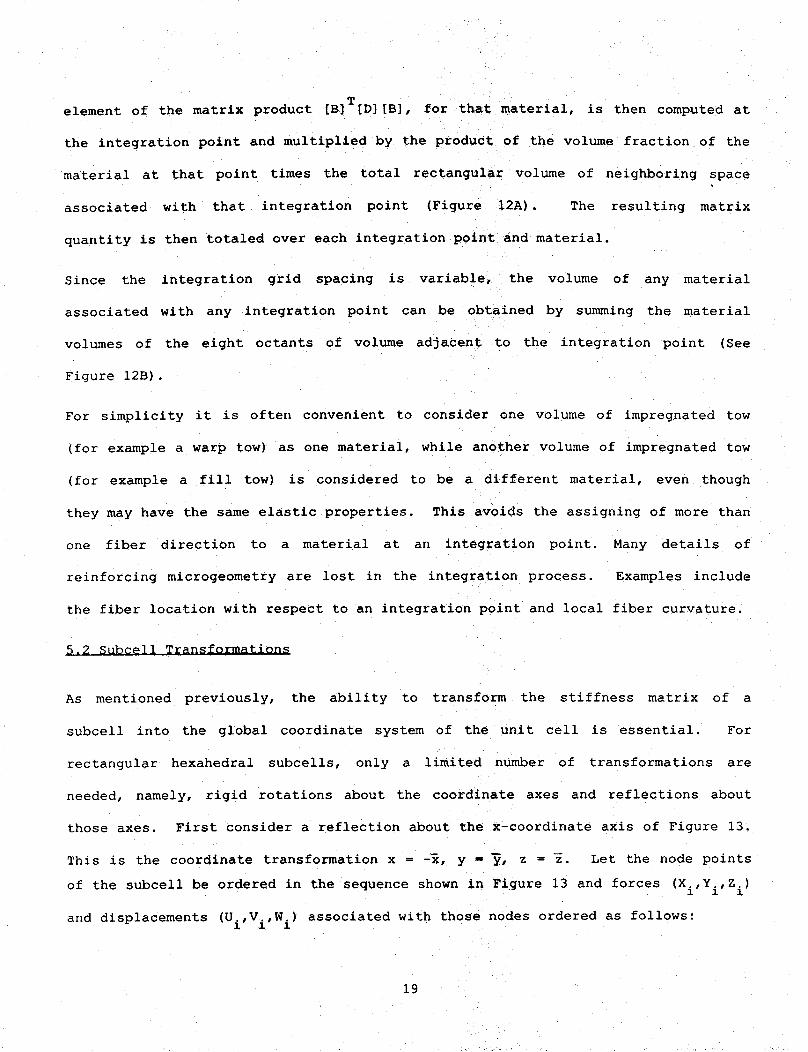
Telement of the matrix product [B] [D] [B], for that material, is then computed at
the integration point and multiplied by the product of the volume fraction of the
material at that point times the total rectangular volume of neighboring space
associated with that integration point (Figure 12A). The resulting matrix
quantity is then totaled over each integration point and material.
Since the integration grid spacing is variable, the volume of any material
associated with any integration point can be obtained by summing the material
volumes of the eight octants of volume adjacent to the integration point (See
Figure 12B).
For simplicity it is often convenient to consider one volume of impregnated tow
(for example a warp tow) as one material, while another volume of impregnated tow
(for example a fill tow) is considered to be a different material, even though
they may have the same elastic properties. This avoids the assigning of more than
one fiber direction to a material at an integration point. Many details of
reinforcing microgeometry are lost in the integration process. Examples include
the fiber location with respect to an integration point and local fiber curvature.
$,2 Subcell Transformations
As mentioned previously, the ability to transform the stiffness matrix of a
subcell into the global coordinate system of the unit cell is essential. For
rectangular hexahedral subcells, only a limited number of transformations are
needed, namely, rigid rotations about the coordinate axes and reflections about
those axes. First consider a reflection about the x-coordinate axis of Figure 13.
This is the coordinate transformation x = -x, y m _, z = z. Let the node points
of the subce!l be ordered in the sequence shown in Figure 13 and forces (Xi,Yi,Z i)
and displacements (Ui,Vi,W i) associated with those nodes ordered as follows:
19
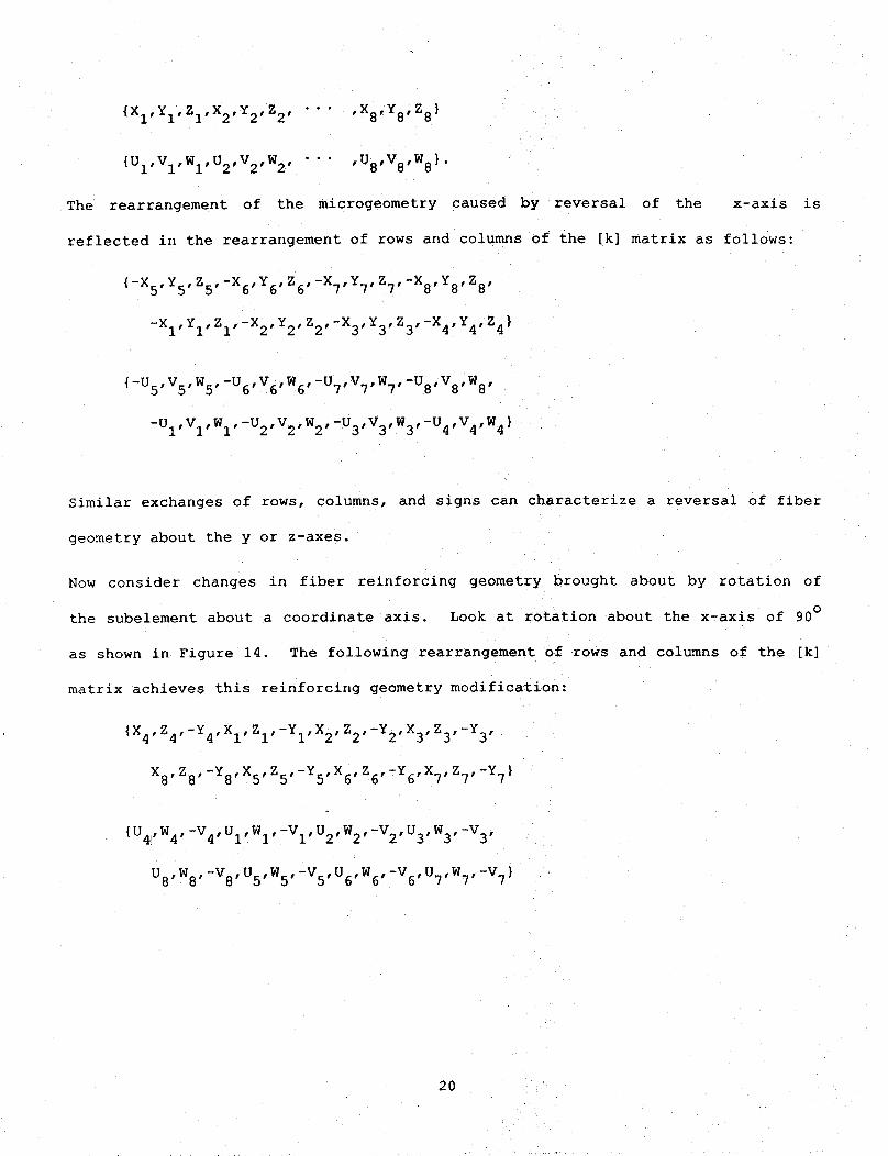
{XI,YI,ZI,X2,Y2,Z2, • " " ,X8,Y8,Z8}
{UI,VI,WI,U2,V2,W2, " • " ,U8,V8,W8}.
The rearrangement of the microgeometry caused by reversal of the x-axis is
reflected in the rearrangement of rows and columns of the [k] matrix as follows:
{-X5,Y5,Z5,-X6,Y6, Z6,-X7,Y7,Z7,-X8,Y8,Z8 ,
-XI,YI,ZI,-X2,Y2,Z2,-X3,Y3,Z3,-X4,Y4,Z4 }
{-Us,V5,W5,-U6,V6,W6,-U7,V7,W7,-U8,V8,W8 ,
-UI,VI,WI,-U2,V2,W2,-U3,V3,W3,-U4,V4,W4}
Similar exchanges of rows, columns, and signs can characterize a reversal of fiber
geometry about the y or z-axes.
Now consider changes in fiber reinforcing geometry brought about by rotation of
the subelement about a coordinate axis. Look at rotation about the x-axis of 90 °
as shown in Figure 14. The following rearrangement of rows and columns of the [k]
matrlx achieves this reinforcing geometry modification:
{X4,Z4,-Y4,XI,ZI,-YI,X2,Z2,-Y2,X3,Z3,-Y3 ,
X8,Zs,-Ys,X5,Z5,-Y5,X6, Z6,-Y6,X7,Z7,-Y 7 }
{U4i,W 4 , -V 4, U 1 ,W 1 , -V 1 ,U 2, W 2, -V 2, U 3, W 3, -V 3,
Us,W 8,-vS,U5,W 5,-v5,U6,W 6,-v6,U7,W 7,-v 7 }
20
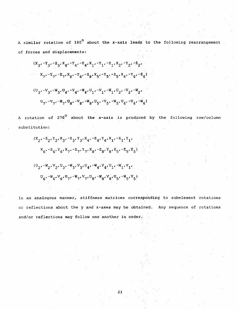
A similar rotation of 180 ° about the x-axis leads to the following rearrangement
of forces and displacements:
{X3,-Y3,-Z3,X4,-Y4,-Z4,Xl,-YI,-Zl,X2,-Y2,-Z 2,
X7,-Y7,-Z7,X8,-Ys,-Zs,X5,-Y5,-Z5,X6,-Y6,-Z6}
{U3,-V3,-W3,U4,-V4,-W4,UI,-VI,-WI,U2,-V2,-W 2,
U7,-V7,-W7,U8,-Vs,-W8,U5,-V5,-W5,U6,-V6,-W6 }
A rotation of 270 ° about the x-axis is produced by the
substitution:
{X2,-Z2,Y2,X3,-Z3,Y3,X4,-Z4,Y4,Xl,-ZI,YI •
X6,-Z6,Y6,X7,-Z7,Y7,Xs,-Zs,Ys,X5,-Z5,Y5 }
following row/column
{U2,-W2,V2,U3,-W3,V3,U4,-W4,V4,UI,-WI,V I,
U6,-W6,V6,U7,-W7,V7,Us,-Ws,Vs,U5,-W5,V5 }
In an analogous manner, stiffness matrices corresponding to subelement rotations
or reflections about the y and z-axes may be obtained. Any sequence of rotations
and/or reflections may follow one another in order.
21

6. ASSEMBLY AND SOLUTION
The process of assembling various subcell stiffness matrices into a unit cell
stiffness matrix is similar to any other finite element assembly. First, nodal
forces and displacements are arranged in some convenient order. Each element of
each subcell stiffness matrix is then placed in its appropriate location within
the unit cell stiffness matrix. All terms in any location of the unit cell matrix
are summed to obtain the unconstrained stiffness matrix of the assembled unit
cell. Now consider the manner in which the nodal displacements are obtained from
the unit cell stiffness matrix, the applied displacements (at corners of the
cell), and the surface boundary conditions.
6.1 Discrete Unit Cell Boundary Conditions
Unit cell corner displacements are established by the particular applied unit
strain and by the location of the zero displacement reference axis. In this
report the unit cell is always located wholly within the positive octant of a
right hand x,y,z coordinate system with one corner of the unit cell at the origin
(Figure 7), the zero displacement reference point. If the unit cell has
dimensions A,B,C in the x,y,z directions respectively, then the eight corner nodes
have the coordinate locations shown in Figure 7. Corner node displacements for
the six average unit strain cases of interest are given in Table i.
Next consider boundary conditions that apply at a finite element node point
situated on either the upper or lower surface of the unit cell, a common point on
two adjacent plies (Figure 8). The nodal boundary conditions are equivalent to
the continuum elastic boundary conditions discussed previously (Section 4.).
Nodal forces at two image points (i,j) must be equal but oppositely directed
(Figure 8), i.e.,
22

X. - -X., Yi " -Y , Z. = -Z. (6.1)I 3 3 I 3
while the corresponding displacement boundary conditions at the same two nodes
are:
Unit Strain Case (I)
Unit Strain Case (2)
E I* W i= ; U, = U.; V. = V ; = Wxx 1 3 1 j j
m
= l*Eyy ; U. " U ; V. = V.; W. = W.1 j 1 3 1 3
Unit Strain Case (3) _ i*zz U i = Uj; V. = V.; W. -C = W.I 3 i 3
= i*" U i = Uj; V. -C = Vj; W i = W.Unit Strain Case (4) yz ' 1 3
= i*; U -C = Uj; V i = Vj; W i = W.Unit Strain Case (5) xz i 3
Unit Strain Case (6) xy ; U. = U.; V i = V ; W. = W.I 3 j 1 3
(6.2)
If there is more than one subcell per ply thickness then there may be node points
on all four vertical faces of the unit cell that are not edge or corner nodes. If
these vertical faces are not planes of structural symmetry then the mixed boundary
conditions at these node points will be similar to those just stated for upper and
lower surface image points. Only the magnitude and location of the constants in
the displacement constraints will differ.
6.2 Discrete Symmetry Boundary Conditions
Where structural symmetry conditions exist on a vertical face of the unit cell,
nodal force conditions become, for all nodes (except corner nodes) on planes of
symmetry perpendicular to the
*All olher average strain c_ts equal zero.
23
x-axis
y-axis
Y = Z = 0X = 0
X= Z = 0Y = 0
for Unit Strain Cases (I), (2), (3) , (4)(6.3)
Jfor Unit Strain Cases (5), (6)
for Unit Strain Cases (I), (2), (3), (5) 1(6.4)
Jfor Unit Strain Cases (4), (6)
Displacement constraints, on planes of symmetry perpendicular to the x-axis, are:
U = 0 (or A) for Unit Strain Case (I)
U = 0 for Unit Strain Case (2), (3), (4) I (6.5)V = W = 0 for Unit Strain Case (5), (6)
For planes of symmetry perpendicular to the y-axis:
V = 0 (or B) for Unit Strain Case (2)
V = 0 for Unit Strain Case (I), (3), (5) (6.6)
U = W = 0 for Unit Strain Case (4), (6)
Similar sets of boundary conditions can be specified for all other unit average
strain cases with the chief difference being size and location of the constant
terms in the displacement constraints. The general form of the system of
equations for nodal forces and displacements can now be written.
6.3 General Statement of the Discrete Problem.
The assembled unit cell stiffness matrix, [K], relates all nodal forces, {F}, and
displacements {6}, as follows:
{F} = [K] {5}. (6.7)
The homogeneous force boundary conditions at surface and edge nodes can be written
symbolically in matrix form as:
{O} = [H] {F} (6.8)
where {O} is the null vector and [H] the coefficient matrix.
The homogeneous and inhomogeneous displacement boundary conditions at surface,
edge and corner nodes can similarly be written in matrix form as:
24

(O,A,B,C}- [J] (_} (6.9)
where {O,A,B,C} is a vector containing only the values O,A,B or C and [J] is the
coefficient matrix. Implicit is the absence of force resultants at all internal
nodes.
The foregoing system of equations (6.7,6.8,6.9) has dimension 6n by 6n where n is
the number of node points in (or on) a unit cell The size of the system can be
substantially reduced before attempting a solution.
All nodal forces must be eliminated by first setting to zero those forces that are
zero in the stiffness matrix. Remaining nonzero force equations involving the
stiffness matrix are then used to eliminate all nonzero force terms from the
homogeneous force boundary conditions. The combination of zero-force stiffness
equations and the force boundary conditions (in terms of displacements) comprise a
set of homogeneous equations in nodal displacement variables only. Each
displacement boundary condition is so simple that it can be used to eliminate one
surface displacement variable in the foregoing set of homogeneous equations. Over
half of the displacement variables on the faces Of the unit cell are eliminated
in this manner. The remaining equations can now be solved for all unconstrained
displacements. The foregoing procedure is not standard finite element procedure.
Most general purpose finite element programs do not treat boundary conditions of
this complexity.
Displacement boundary conditions and corner conditions are then used to obtain
constrained displacement values. All surface and corner forces can be obtained by
substituting the complete set of nodal displacements into the original stiffness
equations. Nodal force components on any side of the unit cell can then be summed
and divided by the area of the side. This dividend is the average stress on that
side. These stress values are the coefficients of the 3-D composite stress/strain
25
law, [D]. Elastic solutions fQr the six unit strain cases provide all 36
coefficients of the stress/strain law which can be inverted to provide the
composite flexibility matrix. Recourse to definitions Df engineering constants
provides formulae for these quantities.
One remaining simplification eliminates the need for reformulating and resolving
each elastic displacement problem for each of the six unit strain cases. Each
unit strain case is considered to be a combination of a homogeneous (uniform)
strain field plus an inhomogeneous (nonuniform) one. Nodal displacements for the
six uniform strain fields are obvious from knowledge of the response of
homogeneous material to uniform surface stress states. The six sets of equations
for the nonuniform displacements turn out to differ only in the inhomogeneous
portions of their algebraic equations. Thus only one large matrix inversion is
required (as opposed to six). If NX is the number of subcells along the x-
parallel side of a unit cell and NY is the number along a y-parallel side then the
size of the inversion is 3[(NX) (NY)-I] square.
The use of planes of structural symmetry to reduce the amount of unit cell
structure that must be analyzed complicates matters somewhat. Strain cases
representing symmetric loads (with respect to planes of symmetry) do not reduce to
the same set (or number) of unconstrained displacement equations as the shear
strain cases which represent asymmetric loadings. Thus, the computational effort
is approximately doubled. Despite this increased effort, it is still advantageous
to use structural symmetry when it exists.
26
7. COMPUTER PROGRAM DESCRIPTIQN
A computer code, based on the foregoing analysis, has been written in Fortran 77
language for use on the CDC 6600 computer at NASA Langley Research Center's
central computing facility. A listing for the program is given in Appendix I.
The core of the program consists of a set of three nested do loops. The outer do
loop computes the stiffness matrix for each elastically different subcell in the
finite element model of the unit cell, transforms it into the global unit cell
coordinates, and inserts each element of the subcell stiffness matrix into its
proper location in the larger unit cell stiffness matrix.
The intermediate do loop ranges over each material within the subcell. In other
words, the subcell stiffness matrix is assembled, one material at a time, and the
contribution that each material makes to the stiffness matrix is computed and
added into the subcell stiffness matrix, which maintains a running total of each
material contribution, in the same manner that the unit cell stiffness matrix
consists, at any point in time, of a running total of the different subcell
contributions.
The third and inner most do loop ranges over each integration point in the
integration grid. The contribution of one material to one subcell stiffness
matrix represents the sum of its contributions at each integration point. As the
fiber directions and constituent material volumes are read in, for any integration
point, the contribution to the appropriate subcell stiffness matrix is calculated
and added into the proper matrix locations. As the last constituent material
associated with the last integration point for the last subcell is read into the
program the last contribution to the unit cell stiffness matrix is put into place
and the unconstrained stiffness matrix of the unit cell is completed. There is no
further input data required. The six unit strain problems are solved in sequence
27
and the mean stresses corresponding to each unit strain tabulated. The elastic
constants for the composite are then computed and displayed.
Prior to entering the nested do loops the necessary information to characterize
the constituent materials, set the number of master subcells, size the unit cell,
divide the unit cell into subcell compartments, and fill each compartment with a
properly transformed subcell, must be specified. The subcells are sized in the
outermost portion of the nested do loops. The input data details are discussed in
Appendix II. Appendix III contains an interactive sample problem input and output
for a simple woven composite architecture. Figure 15 contains a flow chart of the
program.
The math subroutines that invert matrices and solve simultaneous equations (MATOPS
and GELIM) are not included in the listing. Similar subroutines are included in
any math library package.
28
8. SIMPLE APPLICATIONS
In this section fabric analysis is applied to a set of problems that are not
representative of any actual fabric reinforced composite, but are simple enough to
illustrate some basic features of the analysis. The simplest possible application
is the prediction of the stiffness of a bulk orthotropic material, for example, a
graphite/epoxy with the following elastic properties:
Ell = 20.0 msi VI2 = VI3 = 0.25
E22 = E33 = 1.5 msi V23 = 0.35 (8.1)
GI2 = GI3 = G23 = 0.7 msi
where planes perpendicular to the fiber axis are planes of transverse isotropy.
The fiber direction is denoted by I, the direction perpendicular to the fiber (in
the plane of the laminate) by 2, and the ply thickness direction by 3.
The unit cell of this reinforcing geometry can be any size of rectangular prism
with a minimum side length several orders of magnitude larger than the average
fiber diameter. This unit cell can be assembled from a single subcell which
contains only one material, the graphite/epoxy composite with fibers paralleling
the x-axis. The subcell is the unit cell. The simplest 3-D integration grid and
integration scheme is adequate in this case. Let the eight corners of the subcell
be the integration points. The subcell stiffness matrix generated by integration
represents a homogeneous material uniformly distributed throughout the subcell.
The unit cell stiffness matrix is identical to the subcell stiffness matrix.
Subsequent calculation of the composite stiffness coefficients and E,V,G values
yields the same numbers as the material property input. Analyzing the same
material with the fibers at an angle to (rather than parallel to) the global x-
29

axis gives
data.
the composite moduli in a different reference system from the input
8.1
The effect of +45 °
be evaluated with
Fiber Path Variation
zigzag (_) or rickrack fiber paths on the moduli can also
this analysis. For example, consider the 2-D rickrack
reinforcing pattern of Figure 16A. The unit cell shown contains one repeat of
this geometry. The unit cell can be subdivided into two subcells (I and II) with
constant fiber direction in each (Figure 16B). One subcell can be generated from
the other via a 180 ° rotation about the z-axis. Thus only one master subcell and
a pair of rigid transformations are required to orient fibers properly in the unit
cell. Using the previous unidirectional composite properties (Equation 8.1), the
analysis of the unit cell gives the following results:
= = _xzEx = 1.89 msi, Vy z 0.18, Gy z 0.70 msi, ,x = 0
E = 1.50 msi, V 0.35, G 2.04 msi, _xz,yy xz xz
-- -- _xzEz = ].89 msi, Vxy 0.23, Gxy 0.70 msi, ,z = 0
where the coefficient of mutual influence (_ij,k) designates shear strain in the
ij plane as a result of a unit normal strain in the k direction. The comparable
results for unidirectional material oriented at an angle of ±45 ° to the x-axis (in
the xy-plane) without the rickrack pattern are:
E = 1.89 msi, V = 0.18, Gx yz yz
E = 1.50 msi, V = 0.35, Gy xz xz
E = 1.89 msi, V = 0.23, Gz xy xy
= 0.70 msi, _xz,x = 0.81
= 1.40 msi, _xz,y = 0.36
= 0.70 msi, _xz,z = 0.81
3O
The Young's moduli and Poisson's ratios of the rickrack pattern are the same as
the skewed unidirectional material. However, the G shear modulus and all of thexz
non-zero coefficients of mutual influence differ.
Neither of these examples shows how multiple materials can be mixed in the same
subelement. The previous example problem could have been approached in this way;
i.e., the unit cell could have been modeled by a single subcell containing both
fiber angles in the rickrack pattern (see Figure 16C). If half of the subcell
contained only + 45 ° material and the other half -45 ° material then (using the
same eight corner integration points) the volume of material associated with the
four integration points on the x = 0 plane would consist only of +45 ° material
while integration points on the x = A plane would have only -45 ° material
associated with them. The complete subcell stiffness matrix includes all eight
integration points and both + 45 ° and -45 ° material. Resulting moduli predictions
are identical to the previous model based on two homogeneous subcells per unit
cell.
Three-dimensional rickrack reinforcements, shown in Figure 17A, can be analyzed
almost as easily as 2-D ones. A unit cell of this fiber reinforcing pattern is
shown in Figure 17B. Solid lines indicate fiber direction in an entire subcell.
All four subcells (Figure 17C) are rigid transformations of each other. Variation
in Young's modulus of this material with the z-axis fiber orientation angle (for
the same graphite/epoxy) is shown in Figure 18. This figure also contains a plot
of Young's moduli for the 2-D rickrack pattern of Figure 16. Internal constraints
from adjacent subcells increase the 3-D moduli very slightly over the 2-D case.
8.2 Void Analysis
Consider another example problem in which the material is homogeneous and
isotropic except for a periodic array of continuous, parallel, square holes. The
31

major axis of these holes is parallel to the z-axis, as shown in Figure 19A. One
unit cell of this microgeometry consists of a cube of material with one hole in
its center (Figure 19B). Since there is no variation of geometry along the axis
of the hole, there is no need for more than one subelement in that direction. The
simplest conceivable representation of hole geometry is a single subelement with
the volume integration for it's stiffness matrix extending only over the volume of
the actual material present. With the eight corners as integration points, Figure
20 shows the Young's modulus and shear modulus predictions as a function of hole
volume fraction for an epoxy unit cell. Similar estimates may be obtained using
3x3x2 and 4x4x2 integration grids depicted in Figure 21. However, the single
eight-node subcell is not capable of yielding better stiffness estimates than the
rule of mixtures (for elements in parallel) for this example, irrespective of
integration grid refinements.
Now consider a model of the same microstructure with more subcells of smaller
size. The unit cell model in Figure 22 contains 12 subcells. However, only two
are elastically different, the square subcells at the four corners and the eight
rectangular ones between the corners. Stiffness estimates for this model are
shown in Figure 23. Both 2x2x2 and 3x3x2 grids are used for subcell stiffness
integrations. There is a small difference in results for the 2x2x2 and 3x3x2
grids but there is no major improvement in accuracy with this or further grid
refinement. However, a large improvement has resulted from the use of smaller,
more numerous subelements (CompareFigures 20 and 23). The standard of comparison
in Figure 23 is the strength of materials calculation for stretching and bending
of two orthogonal sets of parallel plates, welded together at their lines of
intersection. This model is not an exact solution but is very accurate for hole
volume fractions of more than 50%.
32

For high void fractions, moduli prediction of the fabric analysis and predictions
of the strengths of materials model are generally in agreement; except for the Gxy
shear modulus case. These predictions differ by almost a constant factor of 2.
The reason for this difference is that the G shear modulus is dependent onxy
bending stiffness of the thin cellular walls between the square holes. The eight
node hexahedral element used to represent these cell walls is deficient in its
ability to model linear bending strain distributions.
33
9. WOVEN FABRIC APPLICATIONS
This section considers application of the preceeding analysis to woven fabric
microgeometry. First consider the most common weave construction, plain weave.
Idealizing the geometry is traditionally the first step in analyzing any
structure. For fabrics this usually implies replacing tow bundles with elastic
tubes of constant cross section. In textile mechanics these interwoven tubes are
referred to as channel models (Ref. 18). In composite mechanics these tubes are
assumed to consist of unidirectional orthotropic material with a plane of isotropy
normal to the principal axis of each tube. Figure 24A contains one such
idealization in which tow cross-sections are assumed to have a diamond shape.
Dissimilar materials in the unit cell are separated by a series of flat planar
areas. As mentioned previously, if warp and fili materials and their geometries
are identical, and if a rule of four subcells per yarn crossover is adopted, then
only one master subcell plus 16 transformations of that subcell are required to
model the unit cell, (Figure 24B, C). If a 2x2x2 integration grid is superimposed
on the idealized subcell microgeometry, then the small volumes of dissimilar
materials associated with each integration point can be visualized, characterized,
and tabulated from geometric considerations (Figures 25 and Table 2). Table 2
the two spherical fiber angles (_i,_2) and eight material volumepresents
fractions (Ul, D2,"" • D,8 ) associated with each octant of volume surrounding each
integration point for each of the three constituent materials, namely, the
unidirectional warp composite (I), the unidirectional fill composite (2), and the
bulk matrix (3). The subscripts 1 through 8 on the material volume fractions
refer to the following x,y,z octants respectively: ++÷, ++-, +-+, +--, -++, -+-, -
-+, and as shown in Figure 12.
The volume fraction of impregnated tow in this composite is 50%. The other 50% is
34
interstitial bulk matrix. If elastic properties of the transversely isotopic tow
material have the same values as the unidirectional material of the previous
section (Equation 8.1) and the bulk matrix properties are
E = 0.5 msi, G = 0.185 msi, V = 0.35, (9.1)
then the analytical predictions of the fabric reinforced composite properties are:
E = E = 4.40 msi , E = 1.14 msix y z
G = G = 0.48 msi , G = 0.42 msiyz xz xy
V = V = 0.425 , V = 0.132yz xz xy
If this same graphite/epoxy composite was unwoven unidirectional material in the
form of a thick blended 0/90 laminate with 50% bulk matrix material between the
plies, the laminate properties would be:
E = E = 5.67 msi , E = 1.02 msix y z
G = G = 0.29 msi , G = 0.44 msiyx xz xy
V = V = 0.422 , V = 0.051yz xz xy
The weave microgeometry is thus responsible for an approximate 22% reduction in
Young's moduli E and E , but a much smaller reduction in the in-plane shearx y
moduli.
This sample problem serves only as an example of the application of fabric
analysis to a reinforcing geometry resembling a plain weave microstructure. A
true fabric microstructure has more complex tow paths and tow cross-sectional
variations than this example. However, the analysis is not limited by any of
these geometric complications, as the next example illustrates.
9.1 Realistic Plain Weave Model
Now consider the microgeometry of Figure 26 for a graphite/epoxy, plain weave,
reinforced composite which is magnified approximately 70X. This laminate is an 8-
35

ply composite consisting of T-300 untwisted tow yarns at 18 ends and 18 picks per
inch. The matrix designation is 5208; average thickness per ply is 0.011 inches;
fiber volume fraction is 66.7%. Closer examination of Figure 26 reveals that warp
and fill fibers have a maximum angle of approximately ± 6 ° with the middle plane
of the fabric as they undulate over and under one another. Using the concept of a
somewhat irregular unit cell and subcell of Figure 9 with a 2x2x2 integration
network (the corners of the subcell are the integration points), Table 3 contains
all necessary remaining geometric input data for computation of the subcell
stiffness matrix. As before, _i designates the fraction of volume associated with
the i th octant of volume (surrounding an integration point) that is occupied by
one of the three constituent materials. Octants containing both warp and fill
tows are considered to contain two different orthotropic materials. Bulk matrix
is the third material.
Subcell cross-section sketches and 3-D yarn bundle models, based on
photomicrographs, assist in establishing the _. quantities. For simplicity, fiber1
angles are obtained from observed values at integration points rather than from
averages over neighborhoods of the integration points. There is no attempt in
this example to force reinforcing geometry to coincide with any idealized model.
The fiber volume fraction within a tow bundle is taken to be 75% based on
electronic scanning of similar composite photomicrographs using only those areas
within the tow cross sections. The void content of the composite is assumed to be
zero. The volume fraction of fiber in the tow (75%), times the volume fraction of
impregnated tow within the composite must equal the total fiber volume fraction of
64%.
36
The volume fraction of impregnated tow is thus 85% of the total volume.* The
volume fraction of the composite occupied by unreinforced matrix material must
therefore be 15%. This is necessary to arrive at an overall composite fiber
volume fraction of 64% which is the approximate average measured value for all of
the test materials considered in this section (as determined by acid digestion).
There is some difficulty associated with the assignment of principal moduli to the
impregnated tow material. Neither existing test data or micromechanics provides
reliable estimates. Test data from unidirectional material seldom extends into
the 75% fiber volume fraction range. Also, unidirectional test data does not
include the inevitable degradation to tow properties that result from the weaving
and related fabric forming processes. The latter objection also applies to
micromechanics estimates of moduli. A semi-empirical application of the rule of
mixtures (for elements in parallel) described subsequently seems to provide the
best basis for establishing E 1 of the impregnated tows.
In Ref. 19 twelve different unidirectional graphite composite materials were
characterized experimentally. Their measured longitudinal moduli were lower in
eleven out of twelve cases from the rule of mixtures prediction. The mixtures
rule overestimated measured moduli (E l ) by almost 10% based on an average of the
twelve materials. This shortfall in the measured E 1 can be attributed in part to
fiber loss, misalignment, and breakage in the unidirectional prepregging and
curing processes. The weaving process is considerably more damaging than the
unidirectional prepregging process.
*For analysis purposes 64% fiber volume fraction was used rather than 66.7% because it was desired to have a common
basis of comparison for each of the different weaves in this corrdatiort
37

Thus it seems reasonable to anticipate a greater reduction in E 1 due to weaving
than unidirectional tow placement. Another 10% reduction in E 1 might be
appropriate to account for weaving factors. Therefore, if the fiber volume
fraction of a graphite/epoxy unidirectional material, with a 20 msi longitudinal
modulus, were increased from 65% to 75% the rule of mixtures would predict about a
15% longitudinal modulus increase. However, the weaving reduction factor would
decrease this gain to only 5% and the resulting longitudinal modulus of the
impregnated tow material within the weave would be about 21 msi. A truly reliable
alternative to such an estimate would be an experimental study that measured
impregnated tow modulus before and after weaving. This was beyond the scope of
this program.
The weaving process often includes beaming, sizing, weaving, scouring, drying and
packaging. Each of these steps abrades, damages and misaligns the reinforcing
fibers to some degree. The floor of any weaving room is a testament to the
degradation and loss of reinforcing material. Also, T300 fibers showed more
evidence of property reduction as a result of the unidirectional prepregging
process than most of the graphite fibers studied in Ref. 19.
Only the longitudinal modulus of the tow composite is assumed to be significantly
degraded by weaving. Micromechanics considerations indicate a 15% increase in the
transverse Young's modulus and shear moduli are appropriate to a fiber volume
fraction increase from 65% to 75%. The principal Poisson's ratios should decrease
a few percent as the fiber content increases.
The principal moduli values for the impregnated tow composite are thus estimated
to be (using the Rule of Mixtures for elements in series and parallel):
38
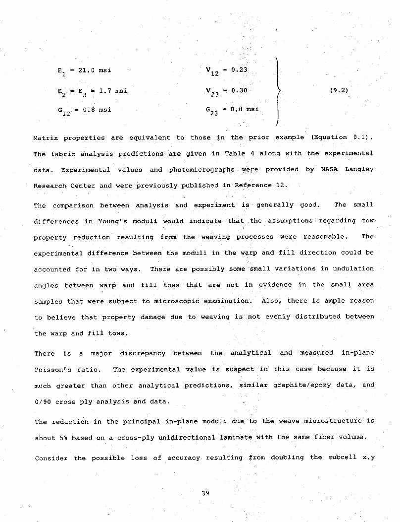
E1 = 21.0 msi
E2 = E3 = 1.7 msi
GI2 = 0.8 msi
VI2 = 0.23
V23 I 0.30
G23 = 0.8 msi
(9.2)
Matrix properties are equivalent to those in the prior example (Equation 9.1).
The fabric analysis predictions are given in Table 4 along with the experimental
data. Experimental values and photomicrographs were provided by NASA Langley
Research Center and were previously published in Reference 12.
The comparison between analysis and experiment is generally good. The small
differences in Young's moduli would indicate that the assumptions regarding tow
property reduction resulting from the weaving processes were reasonable. The
experimental difference between the moduli in the warp and fill direction could be
accounted for in two ways. There are possibly some small variations in undulation
angles between warp and fill tows that are not in evidence in the small area
samples that were subject to microscopic examination. Also, there is ample reason
to believe that property damage due to weaving is not evenly distributed between
the warp and fill tows.
There is a major discrepancy between the analytical and measured in-plane
Poisson's ratio. The experimental value is suspect in this case because it is
much greater than other analytical predictions, similar graphite/epoxy data, and
0/90 cross ply analysis and data.
The reduction in the principal in-plane moduli due to the weave microstructure is
about 5% based on a cross-ply unidirectional laminate with the same fiber volume.
Consider the possible loss of accuracy resulting from doubling the subcell x,y
39
side lengths while reducing the number of subcells in the unit cell from 16 to 4.
One subcell then represents one warp/fill yarn crossover. This increases the
maximum subcell side length ratio from 5/4 to 5/2, which is not excessive for
finite element analysis. If a 3x3x2 integration grid is applied to the subcell
then all the fiber angle and material volume fraction data associated with each
integration point carries over unchanged from the 16 subcell model to the 4
subcell model.
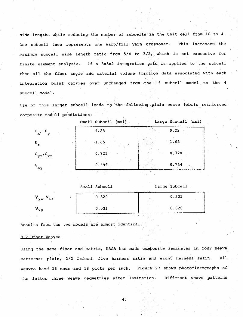
Use of this larger subcell leads to the following plain weave fabric reinforced
composite moduli predictions:
Ex, EY
Ez
Gyz'Gxz
Gxy
Small Subcell (msi)
9.25
1.65
0.721
0.699
Large Subcel! (msi)
9.22
1.65
0.720
0.744
Small Subcell Large Subcell
Iv IVy z,Vxz 0. 329 0. 333
Vxy 0. 031 0. 028
Results from the two models are almost identical.
9.2 Other Weaves
Using the same fiber and matrix, NASA has made composite laminates in four weave
patterns: plain, 2/2 Oxford, five harness satin and eight harness satin. All
weaves have 18 ends and 18 picks per inch. Figure 27 shows photomicrographs of
the latter three weave geometries after lamination. Different weave patterns
40

yield slight variations in fiber undulation angles. The maximum angle that satin
weave fibers make with the plane of the fabric is approximately one degree smaller
than the maximum plain weave fiber angle. Oxford weave angles are smaller than
plain weave angles but larger than satin weave angles. Fiber volume fractions of
the four weaves also vary slightly. In the analysis a fiber volume fraction of
64% was maintained for all weaves.
Figure 28 shows an Oxford weave unit cell and three possible subdivisions. The
first possibility (Figure 28C), with four subcells per yarn crossing, requires 32
transformations of two master subcells to model the unit cell. This model leads
to a matrix inversion of dimension 93 square; probably larger than warranted. The
second possibility (Figure 28D), with two subcells per yarn crossover, leads to a
matrix inversion of order 45. Only 16 transformations of a single master subcell
are required with this model. A third possible model is shown in Figure 28E. It
is a coarser subdivision than either previous model. Each subcell represents one
warp/fill tow crossover. All three models are shown to illustrate the point that
many variations are possible with this type of analysis. The fabric reinforced
composite moduli prediction, based on the medium subcell division model, using a
2x3x2 integration grid, are given in Table 4.
Comparison of the Oxford weave and plain weave moduli predictions shows a slightly
greater Young's moduli for the Oxford weave. This reflects the differences in
yarn crossover angles and crossover frequency. Fiber volume fraction for the
Oxford weave was 64% for the analysis and 62% for the experiment.
Consider the five harness satin weave geometry shown in the photomicrograph of
Figure 27 and the sketch of Figure 29. If a subcell division of the unit cell is
based on a rule of four subcells per yarn crossing then the largest matrix
inversion is of order 297. Use of one subcell per crossover reduces this
41
dimension to 72. Thus, the subcell division shown in Figure 29C was adopted. Two
different master subcell stiffness matrices are required for this model. A 3x3x2
integration grid is used on each subcell. Matrix and unidirectional properties
used are equivalent to those used in the Oxford and plain weave models. Analytical
and experimental moduli are given in Table 4.
Analysis again predicts the trend toward higher in-plane moduli with decreasing
density of yarn undulations. The frequency of undulations has little effect on
shear moduli or Poisson's ratios. Both analytical and experimental fabric volume
fractions of the five-harness satin weave are 64%.
The in-plane Young's moduli correlation is not as good as was obtained on the
plain weave or Oxford weave. This raises a question concerning the use of a
constant unidirectional tow composite property reduction factor to account for tow
damage in weaving. It would appear from the correlation that the amount of tow
damage is a function of the weave style. The lower than expected analytical
Young's moduli for the satin weave, with relatively few warp/fill crossovers per
unit of fabric area, indicates a possible lower level of tow damage than was
evidenced in the plain or Oxford weave forming process with many more warp/fill
crossovers. The beat up process following pick yarn insertion could be more ol a
localized damage phenomenon in the vicinity of warp/fill crossovers than an
overall damage mechanism.
i
The eight harness satin weave is shown in the photomicrograph of Figure 27 and
sketched in Figure 30. One unit cell is shown in Figure 30B. Using four subcells
per yarn crossing leads to a reduced stiffness matrix of 765 square. One subcell
per yarn crossing gives a stiffness matrix of order 189. In addition, three
different master subcells are required. Thus, it is of interest to consider a
42

cruder single subcell that includes four yarn crossovers. Only two different
master subcells require consideration with such a model. This subdivision of the
unit cell is shown in Figure 30C. The unit cell reduced stiffness matrix is of
order 45. Use of the previous constituent material properties with the 5x5x2
integration grid of Figure 30D yields the results given in Table 4.
The lower than expected analytical Young's moduli in the plane of the fabric for
the eight harness satin reflects the same trend as was observed for the five
harness satin and again suggests less weave damage with fewer warp/fill
crossovers.
In general the correlation between analysis and experiment was satisfactory for
most engineering applications. A linearly varying tow property reduction factor
based upon the number of warp/fill crossovers per inch of tow would have very much
improved the correlation. However, this correction should be verified more
thoroghly before adoption.
In summary, a general rule of "four subcells per yarn crossover with crude
integration schemes and networks" is adequate for modeling conventional woven
fabric reinforcing geometries. Larger subcells can be used with little compromise
in accuracy if corresponding refinements are made in the integration network. One
subcell per ply in the thickness direction seems adequate under the same
circumstances.
43

i0. BRAIDED FABRIC APPLICATIONS
A variety of industrial braided fabrics have application as composite reinforcing
materials. Their microgeometries are often similar to woven fabrics. The
simplest 2-D braids (Figure 31A) are analogous to skewed plain weaves.
One important braid characteristic is braid angle, i.e., the average angle (in the
plane of the fabric) that yarns (tows) make with the fabric output (machine take-
up) direction. A braid angle of ± 45 ° corresponds to an orthogonal plain weave
(although some microgeometry differences may result from differences in tow
handling). For analytical purposes ± 45 ° plain braid and plain weave
mlcrogeometry can be considered equivalent. Furthermore, when the braiding tows
are identical and have identical spacing, it is possible to isolate a unit cell
that is a rectangular prism (Figure 31B). This particular unit cell can be
subdivided into four subcells (Figure 31D), each of which can be obtained from the
other by various coordinate transformations. Thus, it is necessary to obtain a
stiffness matrix for only one master subcell in order to model the unit cell. The
stiffness matrix for the subcell is obtained by the same method used for weaves.
First, a 3x3x2 integration grid is superimposed on the subcell volume. Fractional
values of octant volumes (surrounding each integration point) containing the three
constituent materials (two sets of impregnated braid tows and bulk matrix
insterstices) are given in Table 5. Two spherical angles describing local fiber
directions at each of the 18 integration points are also tabulated. This data
corresponds to a braid angle of _ 45 O. The unidirectional composite properties
are given in equation (9.2). Bulk matrix properties are given in equation (9.1).
Moduli predictions for the 64% fiber volume fraction braid and for the 64% fiber
volume fraction plain weave from Section 9. should be close to equivalent after
the plain weave moduli are transformed into the coordinate system of the braid.
44
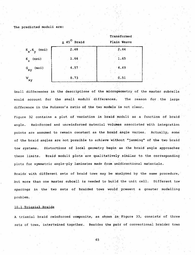
The predicted moduli are:
Ex,Ey (msi)
E (msi)z
G (msi)xy
Vxy
i 45° Braid
2.48
1.66
4.57
0.73
Transformed
Plain Weave
2.44
1.65
4.49
0.51
Small differences in the descriptions of the microgeometry of the master subcells
would account for the small moduli differences. The reason for the large
difference in the Poisson's ratio of the two models is not clear.
Figure 32 contains a plot of variation in braid moduli as a function of braid
angle. Reinforced and unreinforced material volumes associated with integration
points are assumed to remain constant as the braid angle varies. Actually, some
of the braid angles are not possible to achieve without "jamming" of the two braid
tow systems. Distortions of local geometry begin as the braid angle approaches
these limits. Braid moduli plots are qualitatively similar to the corresponding
plots for symmetric angle-ply laminates made from unidirectional materials.
Braids with different sets of braid tows may be analyzed by the same procedure,
but more than one master subcell is needed to build the unit cell. Different tow
spacings in the two sets of braided tows would present a greater modelling
problem.
10.1Triaxial Braids
A triaxial braid reinforced composite, as shown in Figure 33, consists of three
sets of tows, intertwined together. Besides the pair of conventional braider tows
45
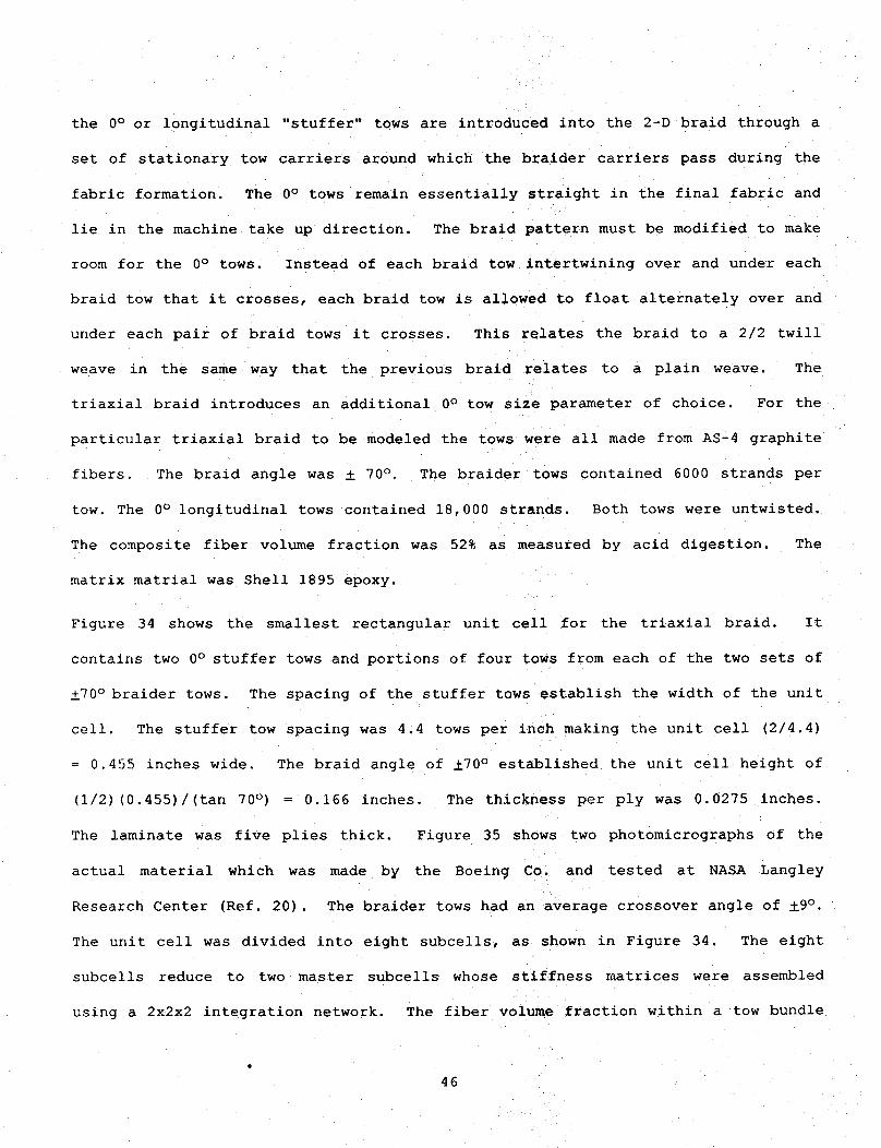
the 0° or longitudinal "stuffer" tows are introduced into the 2-D braid through a
set of stationary tow carriers around which the braider carriers pass during the
fabric formation. The 0° tows remain essentially straight in the final fabric and
lie in the machine take up direction. The braid pattern must be modified to make
room for the 0° tows. Instead of each braid tow intertwining over and under each
braid tow that it crosses, each braid tow is allowed to float alternately over and
under each pair of braid tows it crosses. This relates the braid to a 2/2 twill
weave in the same way that the previous braid relates to a plain weave. The
triaxial braid introduces an additional 0° tow size parameter of choice. For the
particular triaxial braid to be modeled the tows were all made from AS-4 graphite
fibers. The braid angle was ± 70° . The braider tows contained 6000 strands per
tow. The 0° longitudinal tows contained 18,000 strands. Both tows were untwisted.
The composite fiber volume fraction was 52% as measured by acid digestion. The
matrix matrial was Shell 1895 epoxy.
Figure 34 shows the smallest rectangular unit cell for the triaxial braid. It
contains two 0° stuffer tows and portions of four tows from each of the two sets of
±70 ° braider tows. The spacing of the stuffer tows establish the width of the unit
cell. The stuffer tow spacing was 4.4 tows per inch making the unit cell (2/4.4)
= 0.455 inches wide. The braid angle of ±70 ° established the unit cell height of
(I/2) (0.455)/(tan 70 ° ) = 0.166 inches. The thickness per ply was 0.0275 inches.
The laminate was five plies thick. Figure 35 shows two photomicrographs of the
actual material which was made by the Boeing Co. and tested at NASA Langley
Research Center (Ref. 20). The braider tows had an average crossover angle of ±9 ° .
The unit cell was divided into eight subcells, as shown in Figure 34. The eight
subcells reduce to two master subcells whose stiffness matrices were assembled
using a 2x2x2 integration network. The fiber volume fraction within a tow bundle
46
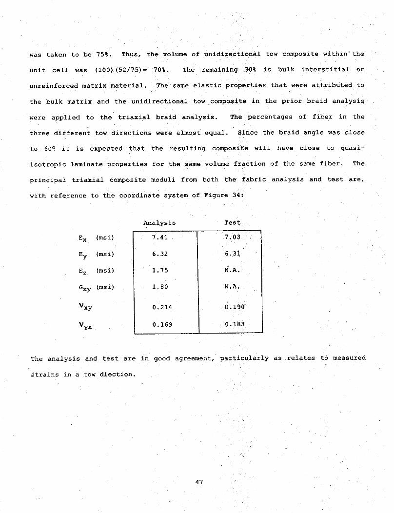
was taken to be 75%. Thus, the volume of unidirectional tow composite within the
unit cell was (100)(52/75)= 70%. The remaining 30% is bulk interstitial or
unreinforced matrix material. The same elastic properties that were attributed to
the bulk matrix and the unidirectional tow composite in the prior braid analysis
were applied to the triaxial braid analysis. The percentages of fiber in the
three different tow directions were almost equal. Since the braid angle was close
to 60 ° it is expected that the resulting composite will have close to quasi-
isotropic laminate properties for the same volume fraction of the same fiber. The
principal triaxial composite moduli from both the fabric analysis and test are,
with reference to the coordinate system of Figure 34:
E x (msi)
Ey (msi)
E z (msi)
Gxy (msi)
Vxy
Vyx
Analysis Test
7.41
6.32
1.75
1.80
0.214
0.169
7.03
6.31
N.A.
N.A.
0.190
0. 183
The analysis and test are in good agreement, particularly as relates to measured
strains in a tow diection.
47
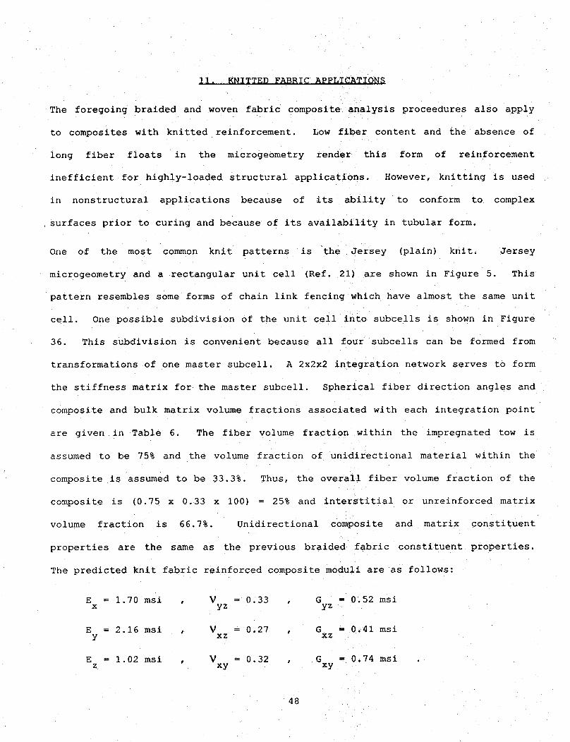
Ii. KNITTED FABRIC APPLICATIONS
The foregoing braided and woven fabric composite analysis proceedures also apply
to composites with knitted reinforcement. Low fiber content and the absence of
long fiber floats in the microgeometry render this form of reinforcement
inefficient for highly-loaded structural applications. However, knitting is used
in nonstructural applications because of its ability to conform to complex
surfaces prior to curing and because of its availability in tubular form.
One of the most common knit patterns is the Jersey (plain) knit. Jersey
microgeometry and a rectangular unit cell (Ref. 21) are shown in Figure 5. This
pattern resembles some forms of chain link fencing which have almost the same unit
cell. One possible subdivision of the unit cell into subcells is shown in Figure
36. This subdivision is convenient because all four subcells can be formed from
transformations of one master subcell. A 2x2x2 integration network serves to form
the stiffness matrix for the master subcell. Spherical fiber direction angles and
composite and bulk matrix volume fractions associated with each integration point
are given in Table 6. The fiber volume fraction within the impregnated tow is
assumed to be 75% and the volume fraction of unidirectional material within the
composite is assumed to be 33.3%. Thus, the overall fiber volume fraction of the
composite is (0.75 x 0.33 x i00) = 25% and interstitial or unreinforced matrix
volume fraction is 66.7%. Unidirectional composite and matrix constituent
properties are the same as the previous braided fabric constituent properties.
The predicted knit fabric reinforced composite moduli are as follows:
E = 1.70 msi , V = 0.33 , G = 0.52 msix yz yz
E = 2.16 msi , V = 0.27 , G _ 0.41 msiy xz xz
E = 1.02 msi , V = 0.32 , G = 0.74 msiz xy xy
48
The in-plane composite Young,s moduli are lower
unidirectional material with the same fiber content.
and Poisson's ratio are higher for the knit.
than (0/90) laminates of
The in-plane shear modulus
In braids, weaves, and knits prestress can distort microgeometry within the unit
cell and cause large changes in moduli of the composite material. Prestretching
of knits in the layup process is almost unavoidable. This phenomena is one reason
for the absence of reliable test data on knits. Figure 37 shows the effects of
prestretching or elongating the unit cell. As in the case of braids, tow
compaction may prevent some of these microgeometries from being achievable.
49
12. CONCLUDING REM_d_KS
This report describes a method for applying general 3-D finite element analysis to
predict all of the linear elastic constants of fabric reinforced composite
laminates. The analysis presumes the reinforcing microstructure can be condensed
into a small repeating rectangular unit cell. The generic composite structure is
presumed to consist of an infinite array of these unit cells joined together at
matching surfaces. The analysis of a single unit cell is sufficient to predict
all the global elastic properties of the composite. The approach avoids some of
the difficulties associated with matching of finite element node point locations
and element boundaries to internal material boundaries. Partially reinforced
elements are used, along with the general energy formula for their stiffness
matrix. This formula accounts for material property variations within the
element. This approach should work if element dimensions are small with respect
to the tow cross-sectional dimensions and interstitial matrix volume dimensions.
This report shows that for many reinforcing geometries it is not essential (within
the requirements of engineering accuracy) that the element size be that small.
With most common reinforcing weaves and with the eight-node hexahedral element, a
general rule for sizing of elements is one element per ply in the thickness
direction and one to four elements per tow crossover. This rule applies to braids
as well. Its application to knits is suggested but unverified.
Since most general purpose finite element codes are awkward to use with the
boundary conditions associated with moduli prediction, a special purpose computer
code was written to facilitate application to these problems. This code is much
quicker and easier to use than general finite element codes. Appendices I, II and
III contain a listing, discussion of input data and sample problem for this
Fortran code.
5O
One advantage to this analysis is that it easily adapts to most forms of
reinforcing microgeometry. The method does not require difficult logic or
multiple option choices and enables the calculation of the all 3-D elastic
contants. Hence, this method is useful for estimating material property inputs
required of impact damageanalysis codes. Another advantage of this analysis is
that it remains within the scope of finite elements, which is familair to many
engineers. No depth of knowledge in textile structures is required.
Examples of application of this analysis to weaves, braids and knits are included
to familiarize readers with fabric microgeometry and modeling of yarn
constructions, and to impart some appreciation for the effects of varying these
construction parameters. It is possible, with this code, to generate a catalogue
of moduli predictions based on microgeometry and constituent property variations.
However, the goal of this report is simply to show that reinforced composite
microgeometry is amenable to routine structural analysis and that this analysis is
useful in the search for impact damageresistant composite designs.
The analytical predictions of fabric reinforced composite moduli have been
compared to test data for several weave and braid reinforced composite laminates.
The predictions are largely within the desired range of accuracy required of most
materials engineering applications.
If a laminate consists of several different plies of different fabrics then it is
necessary to apply the fabric reinforced composite analysis to each different
fabric. This ply level analysis is followed by a conventional laminate analysis
in order to obtain the elastic properties of the complete laminate. Laminates
that are made from many plies of the same fabric reinforcement, oriented at
different angles with respect to each other require a single fabric reinforced
composite analysis followed by a conventional laminate analysis. Thin laminate
51

response may only be approximated using this analysis. Corrections may be
necessary to account for free surface effects and possible single ply bending and
stretching/bending coupling effects.
Historically very few special elements have been developed which contain more than
one material within the elements (except for laminated plate and shell elements).
The potential for new 3-D elements exists within the context of this analysis.
However, this work is beyond the scope of the present effort.
52
1 ,
.
.
°
.
6.
7°
,
9o
I0.
ii.
12.
13.
14.
15.
16.
LIST OF REFERENCES
Wu, Hsi-Yung T. and Springer, G.S., "Impact Induced Stresses, Strains, and
Delaminations", Journal of Composite Materials, Vol. 22, No. 6 (June 1988),
pp. 533-560.
Jortner, J., "Effects of Weave Geometry and Yarn Waviness on Thermomechanical
Properties of Multi-Directional Composites", 3-D Composite Materials, NASA
Conference Publication 2420, (1986), pp 53-73.
Harris, Charles E. and Lee, Jong-Won, "A Micromechanics Model of the
Stiffness and Strength of Laminates With Fiber Waviness", NASA Contractor
Report 181670 (July 1988).
Kriz, R.D., "Influence of Damage on Mechanical Properties of Woven Composites
at Low Temperatures", Journal of Composites Technology & Research, Vol. 7,
No. 2 (Summer 1985), pp 55-58.
Ishikawa, T. and Chou, Tsu-Wei, "Elastic Behavior of Wove_n Hybrid
Composites", Journal o_ Composite Materials, Vol 16 (January 1982), pp. 2-19.
Ishikawa, T. and Chou, Tsu-Wei, "Thermoelastic Analysis of Hybrid Fabric
Composites" Journal of Composite Materials Sciences, Vol. 18 (1983), pp.
2260-2268.
Ishikawa, T. and Chou, Tsu-Wei, "Nonlinear Behavior of Woven Fabric
Composites", Journal of Composite Materials, Vol 17 (September 1983), pp.
399-413.
Ishikawa, Takashi, "Anti-Symmetric Elastic Properties of Composite Plates of
Satin Weave Cloth", Fiber Sciences and Technology, Vol 15 (1981), pp. 127-
145.
Ishikawa, T. and Chou, T.W., "Stiffness and Strength Behavior of Woven Fabric
Composites", Journal of Materials Science, Vol. 17 (1982), pp. 3211-3220.
Ko, Frank K.,; Pastore, C.M.; Yang, J_M. and Chou, T.W., "Structure and
Properties of Multilayer Multidirectional Warp Knit Fabric Reinforced
Composites", Composites 86: Recent Advances in Japan and the United States,
Proc. Japan-U.S. CCM-III, Tokyo, 1986.
Chou, Tsu-Wei, "Modeling and Characterization of Three-Dimensional Braided
Metal-Matrix Composites", 3-D Composite Materials, NASA Conference
Publication 2420, (1986), pp. 31-52.
Dow, Norris F. and Ramnath, V., "Analysis of Woven Fabrics for Reinforced
Composite Materials", NASA Contractor Report 178275 (1987).
Mai, H. Ulv, "A Soft Mosaic Theory for Elastic and Strength Properties of
Hybrid Woven Composites", DFVLR Report B435-85/20 (1985).
Whitney, Thomas J.; Chou, Tsu-Wei; Taske, Leo and Majidi, Azar P.,
"Performance Maps of 3-D Textile Structural Composites", Fiber-Tex 1987, NASA
Conference Publication 3001 (1988), pp. 153-168.
Bathe, Klaus-Jurgen, "Finite Element Procedures in Engineering Analysis",
Prentice-Hall, Inc., Englewood Cliffs, New Jersey 07632 (1982).
Wilson, E.L.; Taylor, R.L.; Doherty, W. and Ghaboussi, "Incompatible
Displacement Models", Numerical and Computer Methods in Structural Mechanics,
Academic Press, Inc., New York, N.Y. (1973).
53
17.
18.
19.
20.
21.
Taylor, Robert L.,; Beresford, Peter J. and Wilson, Edward L., "A Non-
Conforming Element for Stress Analysis", International Journal for Numerical
Methods in Engineering, Vol. 10 (1976), pp. 1211-1219.
Davidson, D.A., "The Mechanical Behavior of Fabrics Subjected to Biaxial
Stress: Channel Model Theory of Plain Weave" A_r Force Materials Lab.
Technical Documentary Report No. MD-TDR-64-23, (July 1964).
Coquill, Scott L. and Adams, Donald F., "Mechanical Properties of Several
Neat Polymer Matrix Materials and Unidirectional Carbon Fiber-Reinforced
Composites", NASA Contractor Report 181805 (April 1989).
Masters, John E.; Foye, Raymond L., Pastore,Christopher M.; and Gowayed,
Yasser A. "Mechanical Properties of Triaxially Braided Composites:
Experimental and Analytical Results", Ninth DOD.NASA, FAA Conference on
Fibrous Composites in Structural Design, Lake Tahoe, NV (November 1991).
Epting, James and Whitney, James, "An Investigation of the Reliability of a
Mathematical Model Which Describes Knitted Fabrics Subjected to Biaxial
Stresses", Air Force Materials Lab. T@chnical Documentary Repot. No. ASD-TD_-
63-450, (June 1963).
54
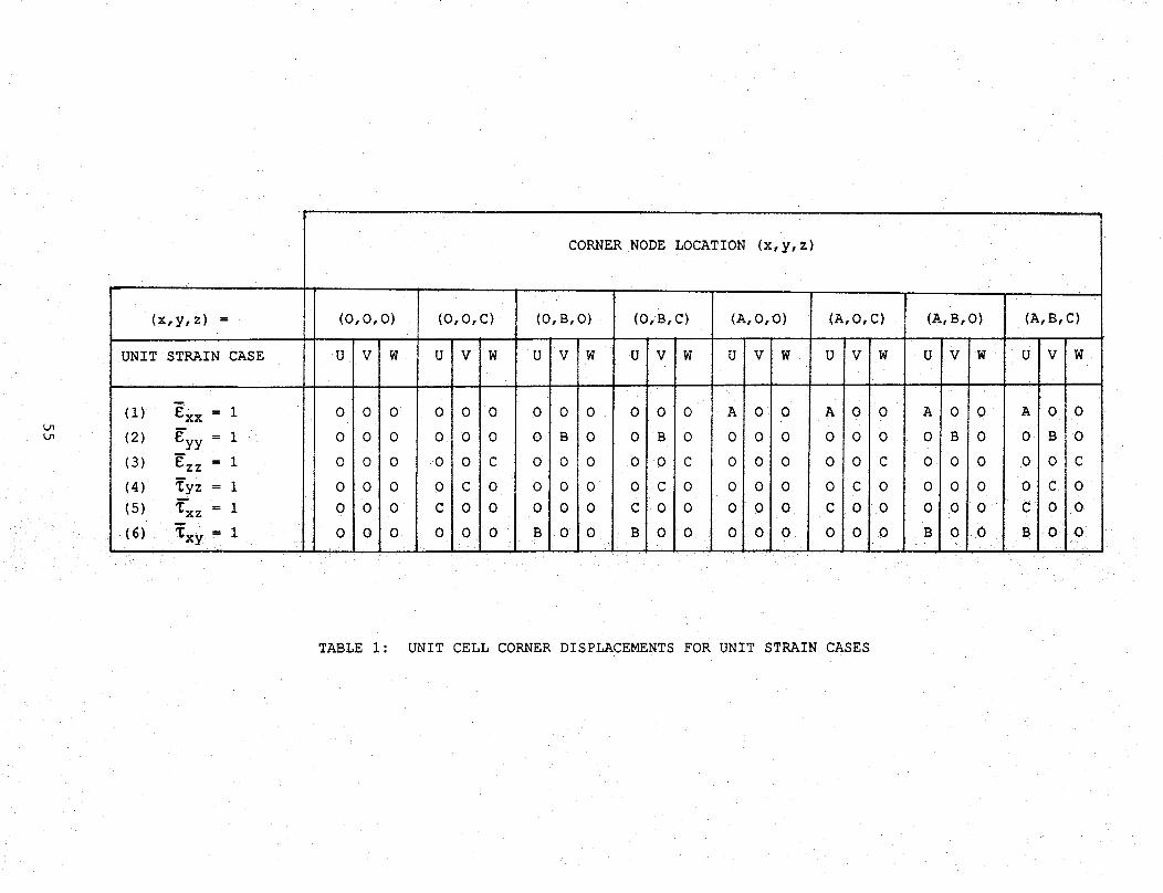
CORNER NODE LOCATION (x,y,z)
Ln
Ln
(x,y,z) =
UNIT STRAIN CASE
(I) _xx = 1m
(2) Eyy = 1
(3) Ezz = 1
(4) _yz = i
(5) _xz 1
(6) _xy; = 1
(O,O,O)
U, V W
0!0 0
0 0 0
0 0 0
0 0 0
0 0 0
0 0 0
(O,O, C)
U!V W
' l
oio o
010 0
00 C
O C O
C O O
O O O
(0, B,O)
U V W
O 00
O B O
O O 0
O O O
O O O
B 010
(O,B,C)
U V W
OIO O
O B O
O O C
O C O
C 00
B O O
(A, O, O)
U V W
A Oi O
000I
000
O O O
O 00
O O O
(A,O, C)
U V W
A O O
O O O
O O C
O C O
C O O
O O OJ
(A,B,O)
U V W
A O O
O .B O
o!o o
0 0 0
0 0 0
B 0 0
(A,B,C)
U V W
A O 0
O B O
00 C
O C O
C O O
O O
TABLE I: UNIT CELL CORNER DISPLACEMENTS FOR UNIT STRAIN CASES
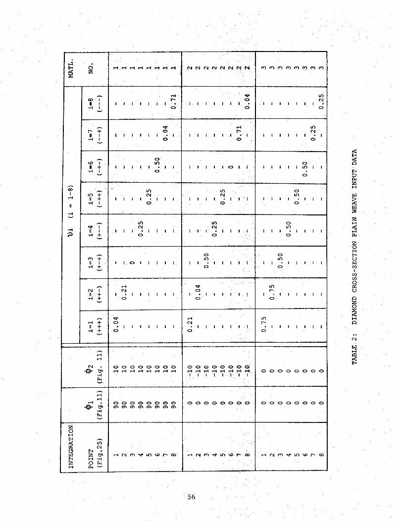
JE_ c;
II I•M I.
v
Ar_ +
II I-M I
v
,.o?It +
•M I
GOA
_+H +
II .,.* i
.Mv
-M
I
r._I I I I I I •
0
IIIIII
c)
I/')I I I I I - I
0
0• I
0
I
A
II I•,-I -t-
v
ur)
I I I I • I I IO
' ' I
tn(N
I I • I I I I0
A(_ +II I
v
II011111
II +•,-I +
v
I i I I I I I0
rM -+- OII + • I I I I I I I
•M + Ov
A
I-I
(N
",'4
A
f'-Ii--I
_-&-Mf-4v
ZOHEl A
L_ E_ •
E_ H -MZ 0H I_
0o000000
oooooooo
I " " i
• i
(Xl e4 Cxl (x; ('xl (xt (xl N
,,_o
I I I I I I I •0
i
u")
oIIIIIII
. i..i ¸¸ ir"
I I I I I I • I0
I I I I I 01 I I
l.n
I I I I • I I I0
I'll011110
, , i
0
I1011111O
OIIII1,!
0
r-I(_
• I I I I I0
It)
I I I I I I • I0
0I I I I _ I I
0
Ou3
I I I I • I I IO
0
_r)I I I • I I I I
0
oIf)
I I 0 I I I I Io
u")
I • I I I I I Io
u')
• I I I I I I Io
0oo00000_ _ _ _ oo0oo000
IIIIIIII
00000000
rl 0,10_ '_ 1.0 kO I'_ GO
_00000000
]
]
[--.iD
ZH
Z
5
Z0I-.IEtU
_0I
U
121Z0
56
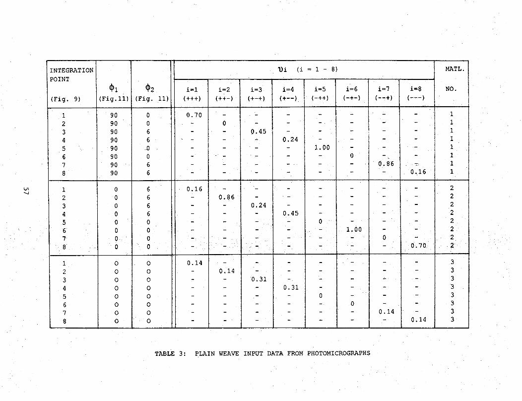
INTEGRATION
POINT
(Fig. 9)
1
2
3
4
5
6
7
8
1
2
3
4
5
7
I, 8
1
2
34
567
8
(Fig. ii)
90 0
90 0
90 6
90 6
90 0
90 0
90 6
90 6
0 6
0 6
0 6
0 6
0 0
0 0
0 0
0 0
O O
O O
O O
O O
O O
O O
O O
O O
i=l
(+++)
0.70
0.16
i=2
(++-)
0
m
0.86
I
_)i (i = 1 - 8)
, . , , ,,i=4 i=5
(+--) (-++)
i=3
(+-+)
0.45
0.24
0.24
0.45
0.31
1.00
0
F
0
i=6
(-+-)
i=7
(--+)
_° o786
l
_2
(Fig. II)
0.14
0
0.14
0.14
0.31
I
1.00
[
0
0.16
0.70
0.14
MATL.
NO.
I
1
I
I
1
1
I
1
2
2
2
2
2
2
2
2
3
3
3
3
3
3
3
3
TABLE 3: PLAIN WEAVE INPUT DATA FROM PHOTOMICROGRAPHS

LnO0
WEAVE
Plain
Oxford
5 Harness
Satin
8 Harness
Satin
Ex
(ms i )
9.25
(9.13)
9.33
(9.63)
9.57
(10.05)
I 9.68'(10.59)ii
Ey
(msi)
9.25
(8.83)
9.55
(9.68)
9.57
(10.09)
9.68
(10.35)
Gyz
(msi)
Gxz
(msi)
x,y plane is the plane of the fabric
* Warp Direction
** Fill Direction
*** Thickness Direction
Gxy
(msi)
0.7O
(N.A.)
0.70
(0.77)
, Vyz Vxz Vxy
0.03
(0.ii)
0.04
(0.06)
0.72
(0.76)//
0.72
(0.98)
0.03
(O.O6)
0.03
(0.06)
( ) Experimental Data
(N.A.) Not Available
Table 4: WOVEN FABRIC RESULTS

ha%(
INTEGRATION
POINT
1
2
3
4
5
6
7
8
9
I0
ii
12
13
14
15
16
17
18
Integration Points
l)i (i = i-8)
i=3 i=4 F i=5 i=6 i=7!
(+-+) (+--) I (-++) (-+-) (--+)
i- 0.9 / - - -
0.4 .... /
- 0.4 - - -
- - - 0.9 -
0.2 - 0.2 - -
- 0.2 I - 0.2 -
- - | - 0,4 -
- - _ 0.9 - 0.8
Subcell
TABLE 5A: BRAID INPUT DATA (MATERIAL i)
I
0.3
O
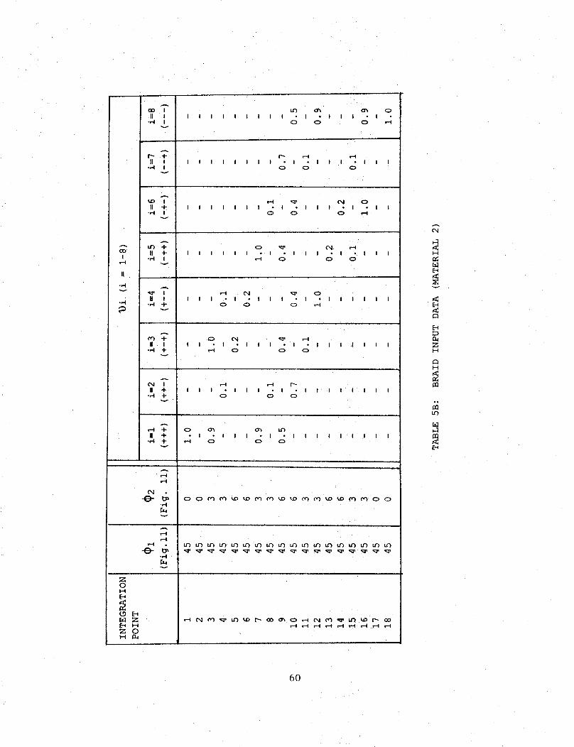
A
CO I
II i• M I
r-- 4-II I
-,-I I
lllillill
O's
• I • I I I - I
0 0 <_,
_TII 4-
..-I I
llllllll • I • I I I • I0 0 0
I I
A
ur) +
CO II +
I -M I
II
.,..t
v _ "TII I
.,-t -,'4 +
IIIIII I • I • I I I I
0 0 O
0
I I I I I I • I
I--I 0
('hi. _'4
I I I • I .. I I I
0 0
I I
_ ,m3' 0
I • I • I I I - I " I I I I
O C) O
I I
A
,n+-) +II i
-M 4-
I IC)
• I • I I
r.-I 0
I • I - I I I I I I I
0 0
0+
C_I "_ r_l ,--'1 I'_
II + I I I . I I I I - I I I I I I I I--4 + 0 C:_ 0
+-'4 -I- C) O_ 0% U')
II + - I - I I I . I - I I I I I I I I I
-+4 Jr _ 0 C) E)
, i
A
C,I
"M
v
A
_-&-,.4
v
0 0 _ _ _ _ _ _ _ _ _ _ __ 0 0
, , , l
_ _ _ _ _ _ _ _ 0 _ _ _ _ _ _ _
Z0I-4
E_
L_Z
__ HZ 0H 1_
H
E+
v
ZH
H
¢n
6O
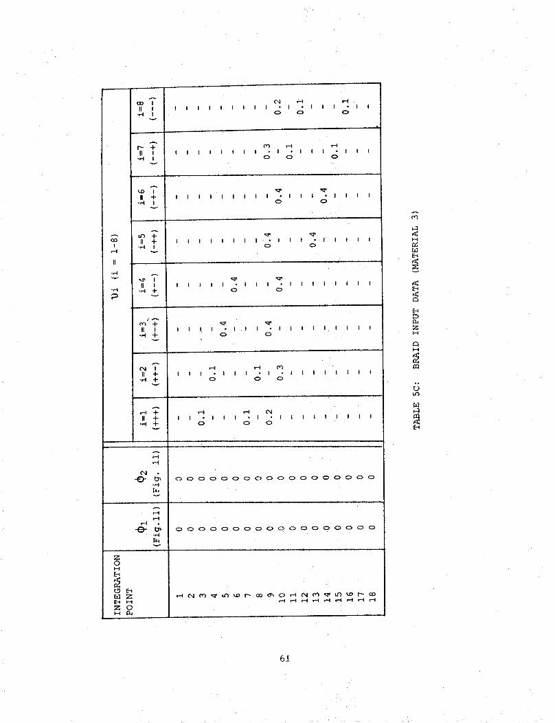
!I-4
I1
.,-I
.-4
zOHE_
[.9 £-_
Z
Z 0
II I-,-4 I
v
r- +
II I•,-I I
IIIIIII1"1"111"110 0 0
IIIIII(_ r-4
I !0 0
I I I
,oi"II +
•M Iv
I I IIIIll I
Aur) +
II +-M I
II !
lillllll • I I Io
_P• I I I I I
o
I I I I I • I0
I I •o
IIII IIII
_Aor) +
II I-,..I +
I I I I • I I I0
C:_ I I I I I I I I I
II +•M -l-
v
I I I,-"4 ,-4
• I I I • I0 0
IY)• 1 I I I I I I I
C)
A
II +•,-I +
I I o¢n1
i i I • i • i i i i I i I I io o
.,-i
_-&-,4r,4v
000 C) 000000000 O 0000
..... , ., ,l , ,,
000000000000000000
___0___
,--1
H
r.'l
v
Z
A
m
S
61
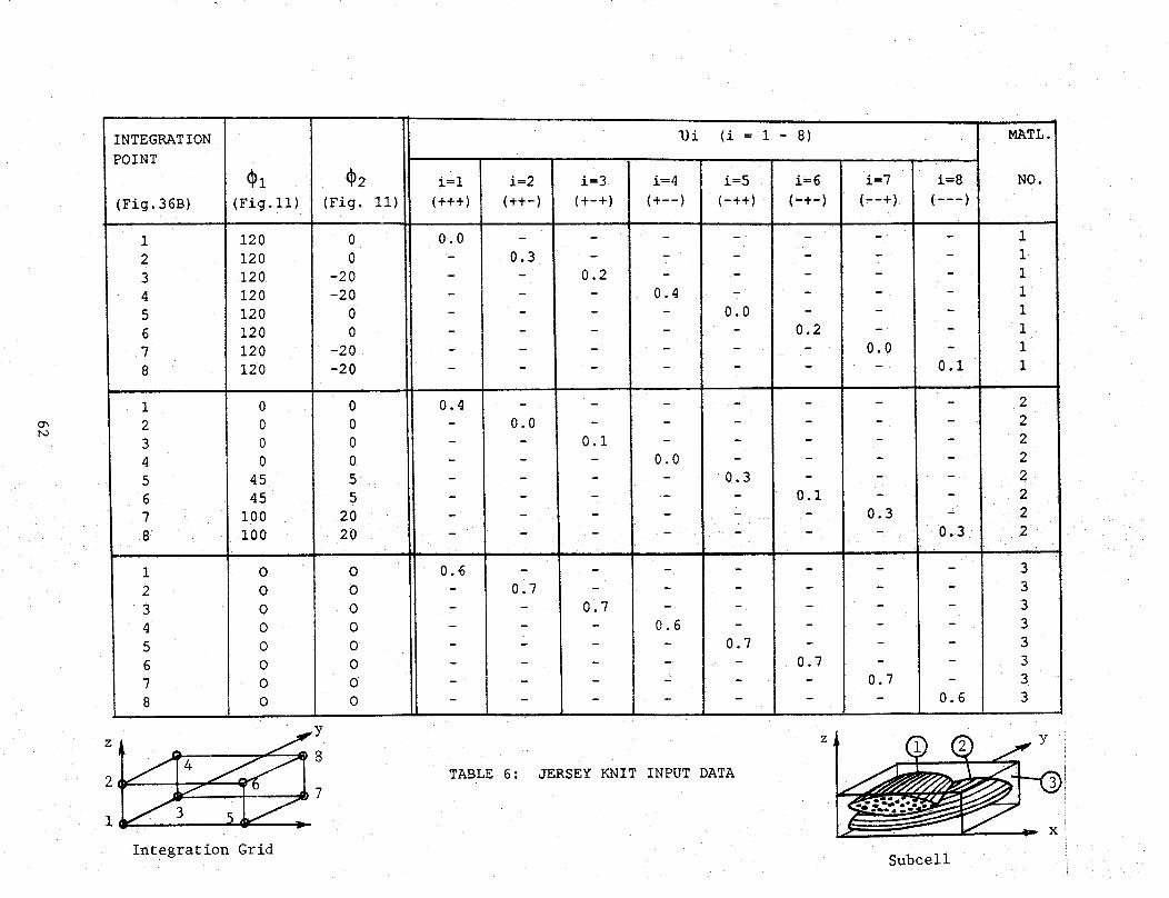
O_50
INTEGRATION
POINT
(Fig.36B)
1
2
3
4
5
6
7
8
1
2
3
4
5
6
7
8
1
2
3
4
5
6
7
8
(Fig. ii)
120
120
120
120
120
120
120
120
O
O
0
0
0
O
O
O
_2
(Fig. Ii)
0
0
-20
-20
0
0
-20
-20
0
0
0
0
5
5
20
20
0
0
0
0
45
45
I00
I00
0
0
0
0
0
0
0
0
i=l
(+++)
0.0
0.4
0.6
_)i (i = 1 - 8)
i=2
(++-)
0.3
0.0
0.7
i=3
(+-+)
0.2
0.I
o 7
i=4
(+--)
0.4
0.0
0.6
i=5
(-++)
II -
0.0
0.3
- 0.1
I
-- [ --
0.7
- 0.7
i=6
(-+-)
0.2
i=7
(--+)
0.0
0.3
0.7
i=8
(---)
I
0.1
0.3
0.6
MATL.
NO.
i
1
1
1
1
1
1
1
2
2
2
2
2
2
2
2
3
3
3
3
3
3
3
3
Integration Grid
TABLE 6: JERSEY KNIT INPUT DATA
Subcell
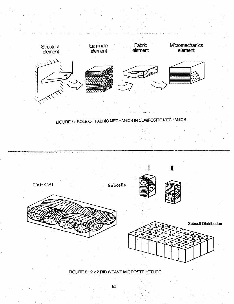
Structural Laminate Fabricelement element element
_\\\\\\\\" i; -7"/.,9_
VJ../_//'JJ_q(,flll//#_
_///////////////I__
Micromechanicselement
FIGURE 1" ROLE OF FABRIC MECHANICS IN COMPOSITE MECHANICS
. L • .............. ' ' . '
]I
Unit Cell Subcells _
Subcell Distribution
FIGURE 2:2 x 2 RIB WEAVE MICROSTRUCTURE
63
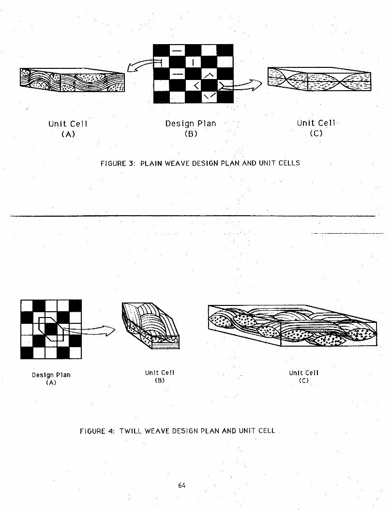
Unit Cell
(A)Design Plan
(B)
Unit Cell
(c)
FIGURE 3: PLAIN WEAVE DESIGN PLAN AND UNIT CELLS
Design Plan Unit Cell Unit Cell(A) (B) (C)
FIGURE 4: TWILL WEAVE DESIGN PLAN AND UNIT CELL
6A

2 x 2 Warp Rib Weave
i'iii
| i
lae
i
:,!i
ZZZZ
"ZZZ.
"4
2-D Braid
.......... i t i i i°=_.Q.... i.o°o_ .... | I i
i,',:,:,' .........
jii,....,,,"""""""....,.2 x2 Basket Weave
5-D Braid
Jersey Knit
1Tricot Knit
FIGURE 5: UNIT CELLS FOR WEAVES, BRAIDS, AND KNITS
6.5
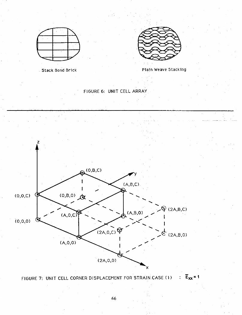
Stack Bond Brick Plain Weave Stacking
FIGURE 6: UNIT CELL ARRAY
z
I(O,O,C)
(0,0,0)
FIGURE 7:
(O,B,C)
(A,O,O)
(A,B,C)
(2A,O,O)
m
UNIT CELL CORNER DISPLACEMENT FOR STRAINCASE (i) " Exx =1
66
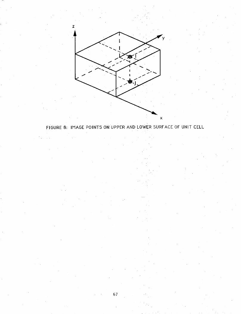
FIGURE 8:
X
IMAGE POINTS ON UPPER AND LOWER SURFACE OF UNIT CELL
67

1
5
Material (3)
Material (2)
Material (I)
Subcell
Unit Cell
Subcell Assembly
FIGURE 9: PLAIN WEAVE GEOMETRY
68
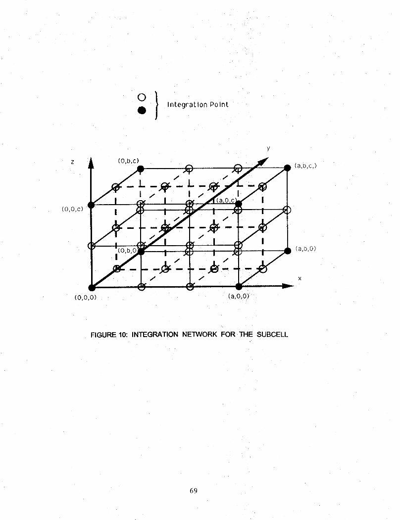
Integration Point
(O,O,c)
(O,b,c)(a,b,c,)
,__,_ , ..,_/ i I" " "
,_ I _ (a,b,O)
(0,0,0) (a,O.O)
FIGURE 10: INTEGRATION NE'IWORK FOR THE SUBCELL
69
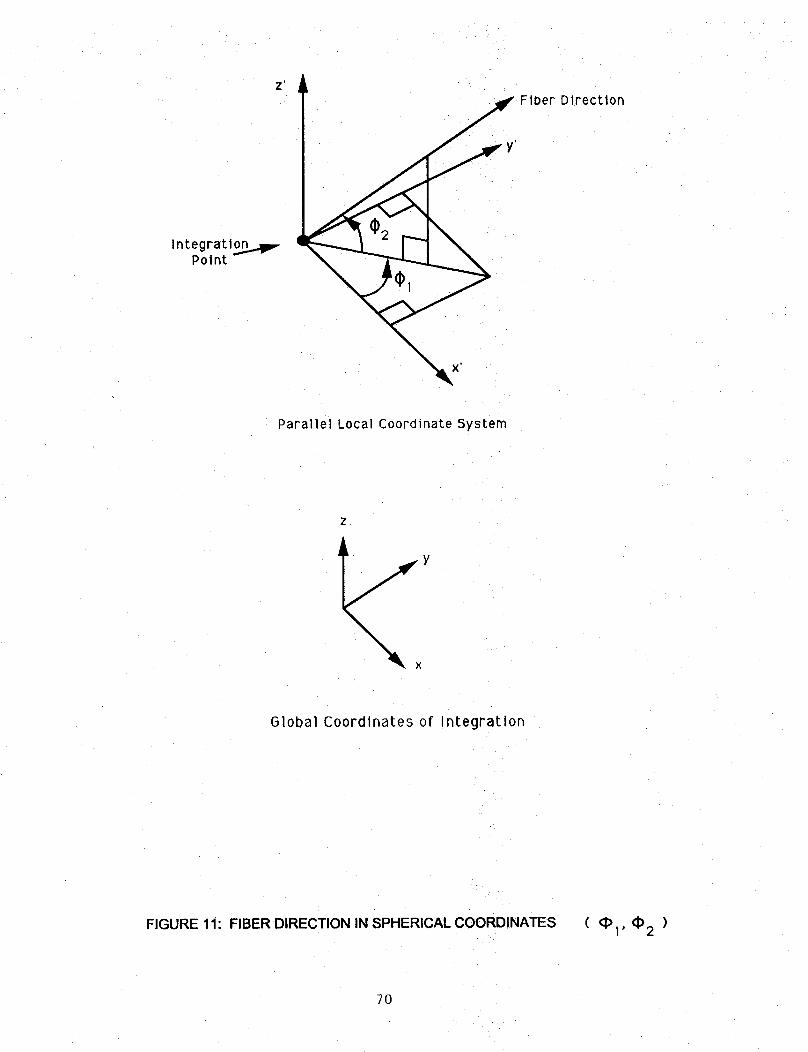
Z'
Integratlo_Point
Fiber Direction
Parallel Local Coordinate System
Y
Global Coordinates of Integration
FIGURE 11: FIBER DIRECTION IN SPHERICAL COORDINATES (q) 1' (I) 2 )
7O
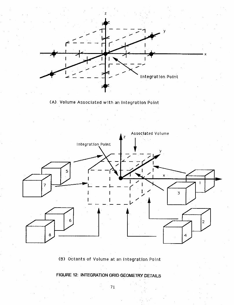
Z
111- _ ..-"1_. yI I_./ t
_- _ ._ _ o
×
eg tlon P
(A) Volume Associated wlth an Integration Point
A z Associated Volume
Integration.Point _ _ Y
I_.__ I ii /
/ /
I I(B) Octants of Volume at an Integration Point
FIGURE 12: INTEGRATION GRID GEOMETRY DETAILS
7]
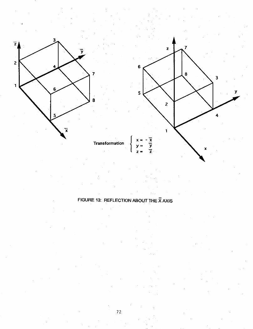
24
7
8
Transformation
6
8
4
FIGURE 13: REFLECTION ABOUT THE X AXIS
72
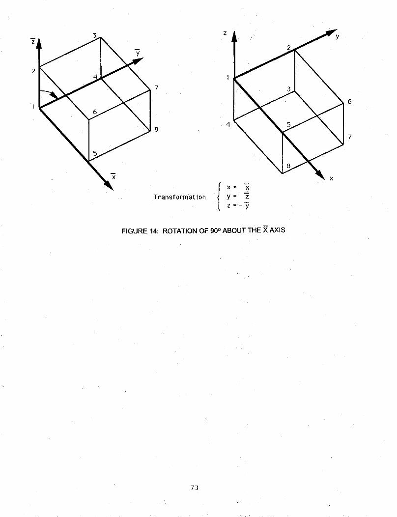
y
Transformation
4
g
×= ×
y= 7
z=-y
Y
6
7
×
FIGURE 14: ROTATION OF 90 ° ABOUT THE X AXIS
73
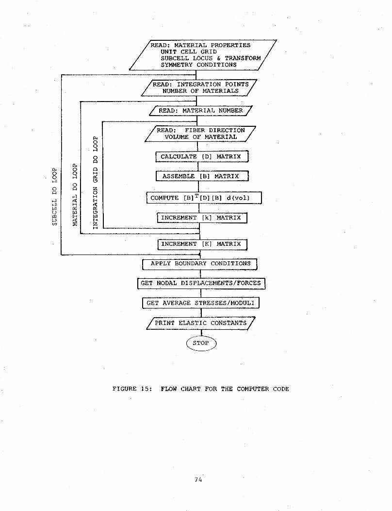
oo,-]
o
,._.],-IHt)l:n::DIn
o
o
<H
oo,-]
o
cII-.-I
(_9
:ZOI-I£-a
t9
[-4Zi---t
READ: MATERIAL PROPERTIESUNIT CELL GRID /SUBCELL LOCUS & TRANSFORM/SYMMETRY CONDITIONS , ,/
oiREAD:INTEGRATIONPOINTS/NUMBEROF MATERIALS/
I
]I
/READ: FIBER DIRECTIONVOLUME O F MATERIAL /
I!CALCU_TEtD1MATRIX]
I[ ASSEMBLEIBIMATRIX|
I[,C?MPUTE[B]T[D] [B] d(vol) I
I[ INCREMENTIkJ MATRIX]
INCREMENT [K] MATRIX I
4[ _P_,.YBO_''DARYCO'D'T'ONSI
I[GETNODALDISPLAC_.MENTS/FORCES1
I[GETAv_._GESTRESSES/MODU',"]
!/_IN,_._,c_o,s,_,,s/
FIGURE 15: FLOW CHART FOR THE COMPUTER CODE
74
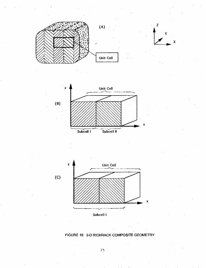
_ m m m •
_\'x_>A;- -: :'4mXs
• ,* Q,. •
;i:il onc
Z
(B)
Unit Cell
Subcell I Subcell II
(c)
z II1 Unit Cell
/
Subcell I
FIGURE 16: 2-D RICKRACK COMPOSITE GEOMETRY
75
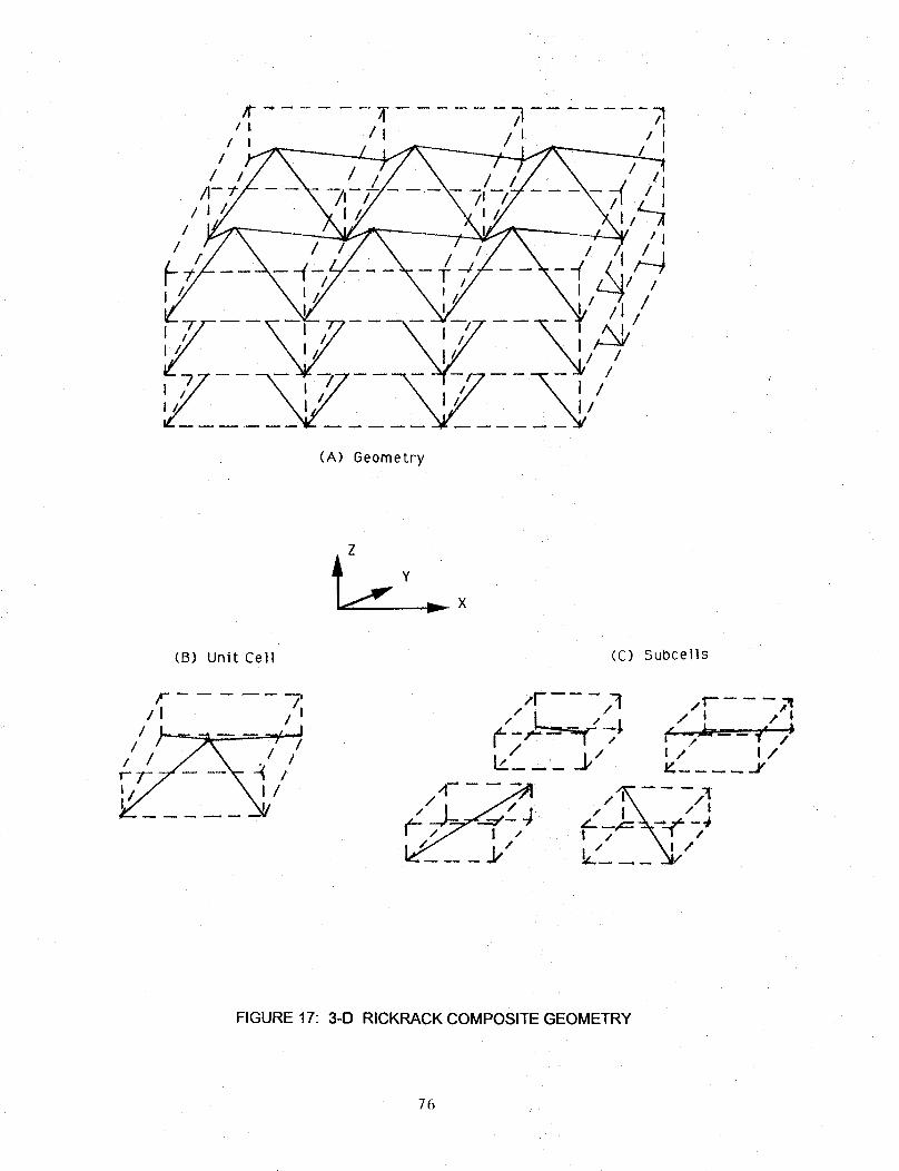
IL II /it /iI . - _- - .-'--_ - --- I I 1
I /A-//- % - ',,_z/__ ____/_/J__ _\__: ,'!
i _i:_-_ --_" _"i
,.7 \:]/ \;// \;z _ IIL__ _____',Z_....... _ ....... _ I ,"
CA) Geometry
(B) Unit Cell (C) Subcells
FIGURE 17: 3-D RICKRACK COMPOSITE GEOMETRY
76

Z
c 2-D Subcell
2O
3-D Subcell
z y
c Fiber ion
@2
E Z
(msl)
!0
3-D
2-D
I I I I i I! 5 30 45 60 75 90
@2 (degrees)
FIGURE 18: MODULUS OF RICKRACK COMPOSITE
77
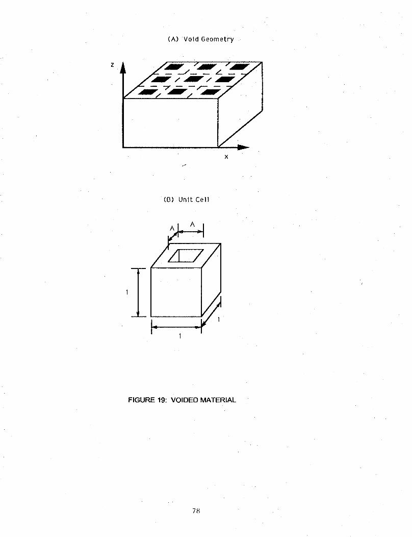
(A) Vold Geometry
x
i
(B) Unlt Cell
A A
--7-
1
1
FIGURE 19: VOIDED MATERIAL
7_
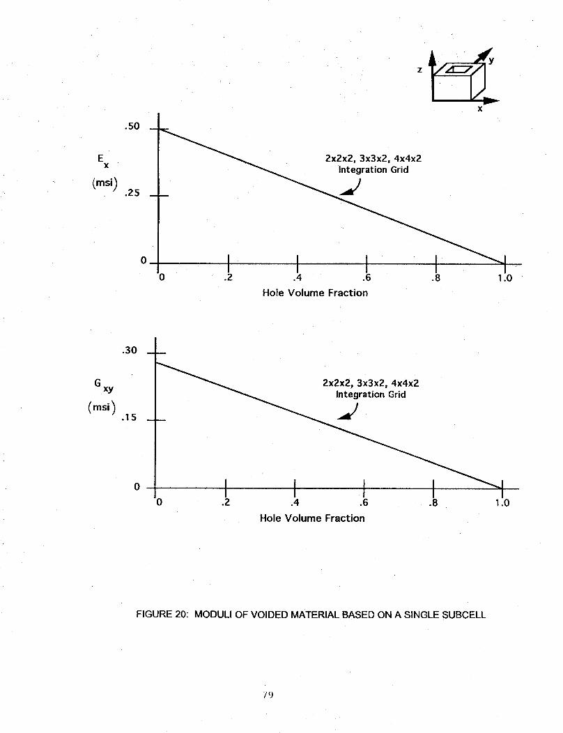
EX
.50
.25
0
X
--__ 2x2x2, 3x3x2, 4x4x2
IO .2 .4 .6 .8 1.0
Hole Volume Fraction
.30
2x2x2, 3x3x2, 4x4x2G xy Integration Grid
(msi) .15 ____ J
0
0 .2 .4 .6 .8 1.0
Hole Volume Fraction
FIGURE 20: MODULI OF VOIDED MATERIAL BASED ON A SINGLE SUBCELL
79
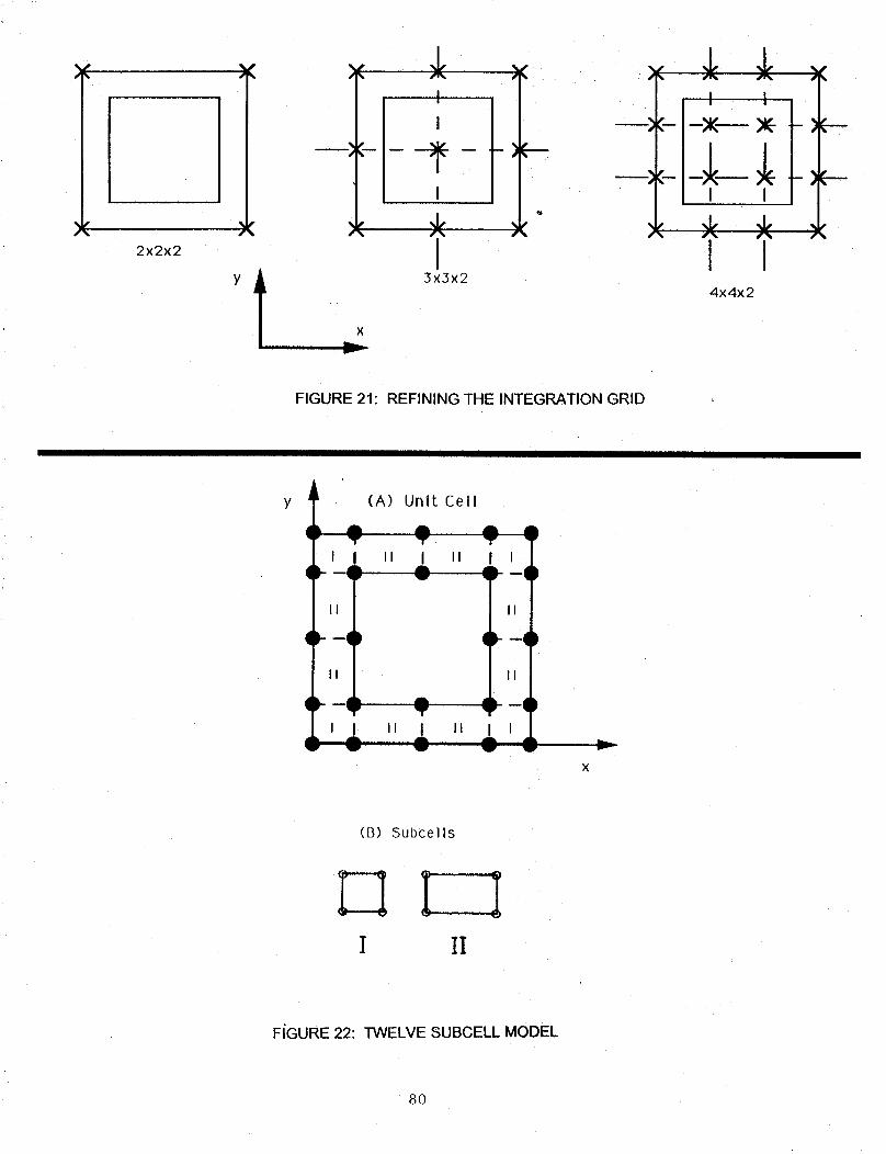
)(
2x2x2
) %
, I
]
---_-
I
),'
)_--
I3x3x2
%
), ,I,
I
• ,L ,LI I
I I
,J,,
I4x4x2
%
FIGURE 21" REFINING THE INTEGRATION GRID
I I I
(A) Unit Cell
k A l• _lF T
r I ii I
F-#l w"'
_-0
I d
@-(
II I
)___ AT
i I iJ IW V
II
i II
0-(
III
ql'
I tA •
V I Um_
x
(B) Subcells
I II
FIGURE 22: TWELVE SUBCELL MODEL
8O
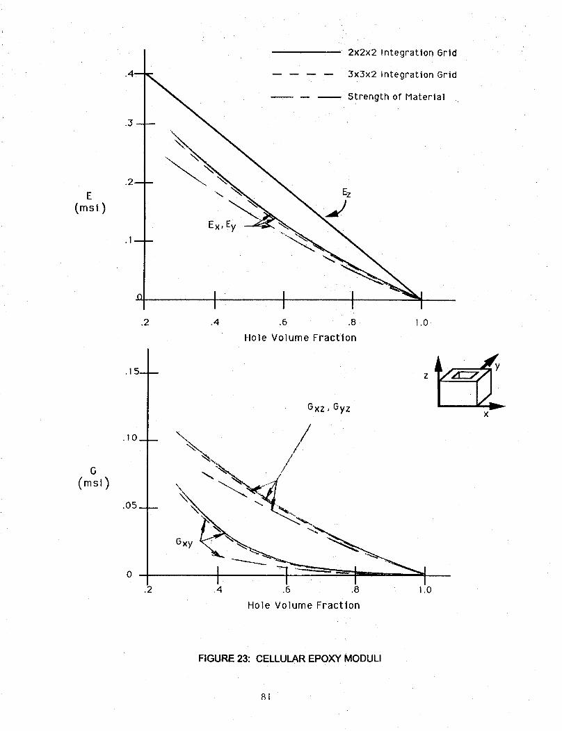
2x2x2 Integration Grid
3x3x2 Integration Grid
Strength of Material
E
(msl)
Ez
Ex, Ey
I.2 .4 ,6 .8 1,0
Hole Volume Fraction
.15--
.iO_
.05 _
Gxz, Gyzx
\\. j11/
_...
.4 .6 .8 1,0
Hole Volume Fraction
FIGURE 23: CELLULAR .EPOXY MODULI
8.1
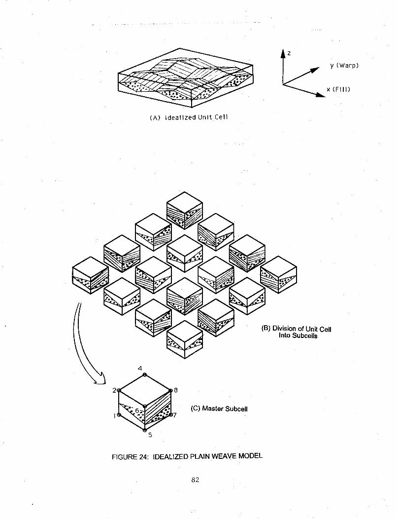
(A) Idealized Unit Cell
y (Warp)
x (Fill)
4
5
(C) Master Subcell
(B) Division of Unit CellInto Subcells
FIGURE 24: IDEALIZED PLAIN WEAVE MODEL
82
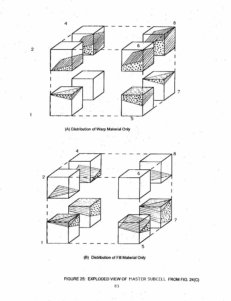
2
,4
5
8
7
(A) Distribution of Warp Material Only
8
2 rZ
7
15
(B) Distribution of Fill Material Only
FIGURE 25: EXPLODED VIEW OF MASTER $UBCELL FROM FIG. 24(C)
83
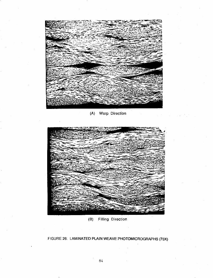
(A) Warp Direction
(B) Filling Direction
.FIGURE26: LAMINATEDPLAINWEAVEPHOTOMICROGRAPHS(70X)
84
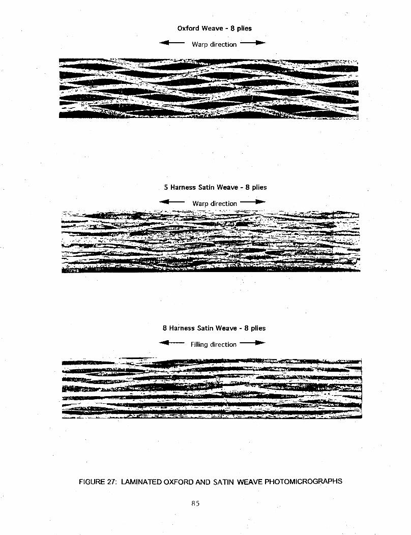
Oxford Weave - 8 plies
Warp direction
5 Harness Satin Weave - 8 plies
Warp direction
8 Harness Satin Weave - 8 plies
Filling direction
_ "_e - , T-"
FIGURE 27: LAMINATED OXFORD AND SATIN WEAVE PHOTOMICROGRAPHS
85
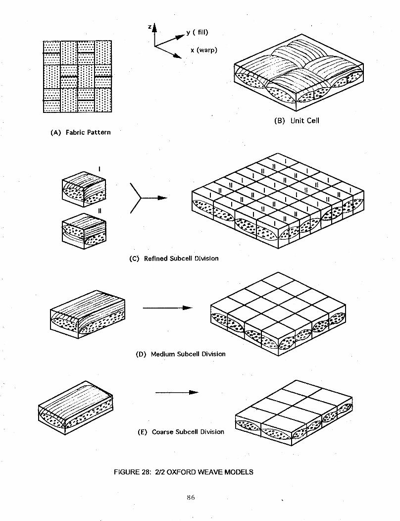
.... =.
/
'111 i
:,:0 ,I°:0'.-.-.-.- -.
m
|-°-i ...... °;1_°
,:,:,1 :,:,:_,00=0i
J°|=° i,'o'. :!:
.....iaiio oliOi _I °I ii|°o
,o, o:,:,°1°11°°lli m°°°°= II=°lilo
Iiil°,:,:° ,oI°1 |11I_t_4 oO,°,
(A) Fabric Pattern
Z_y (fill)x (warp)
(B) Unit Cell
(C) Refined Subcell Division
eh=..=y
(D) Medium Subcell Division
me=.._v
(E) Coarse Subcell Division
FIGURE 28:2/2 OXFORD WEAVE MODELS
86

iii_iii!_i!i!liiiiililiiiiliiiii_i__!il_:_-:_-:_-:li!!iiiiili_iii_!i_i!iiliiiiEiiii,.'-T-"" .....
°_ °°'° ::°°",
(A) Fabric Pattern
(B) Unit Cell
(C) Subcell Dlvislon
FIGURE 29: FIVE HARNESS SATIN WEAVE MODEL
87
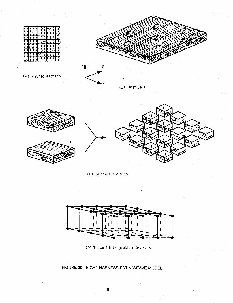
! !i_H!i:li_t!it!!i "
i:,'--1!i il:ili: t:i Ii;!! .... :1,':i_lii!li::l!it_ t'::"
iiil!i!F:-.'-llili.I:!:i_l;--..ilil!iili!il!ifill_I
(A) Fabric Pattern
(B) Unit Cell
(C) Subcell Division
(D) Subcell Intergration Network
FIGURE 30: EIGHT HARNESS SATIN WEAVE MODEL
88
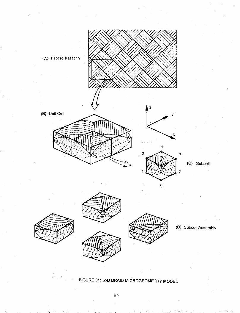
(A)
(B)
FabricPattern _j,/,__ x
UnitCell
2 8
(c)
1 7
Subcell
(D) Subcell Assembly
FIGURE 31" 2-D BRAID MICROGEOMETRY MODEL
89
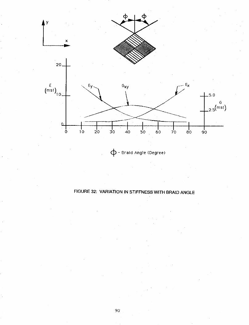
TY x
20_
E
(mSl)l 0 - _
0I̧ -¸ i....T_I I J I iI
I 0 20 30 40 50 60 70 80
__ __5.0
G
i2.5 (mSi)
9O
(_- Braid Angle (Degree)
FIGURE 32: VARIATION IN STIFFNESS WITH BRAID ANGLE
90
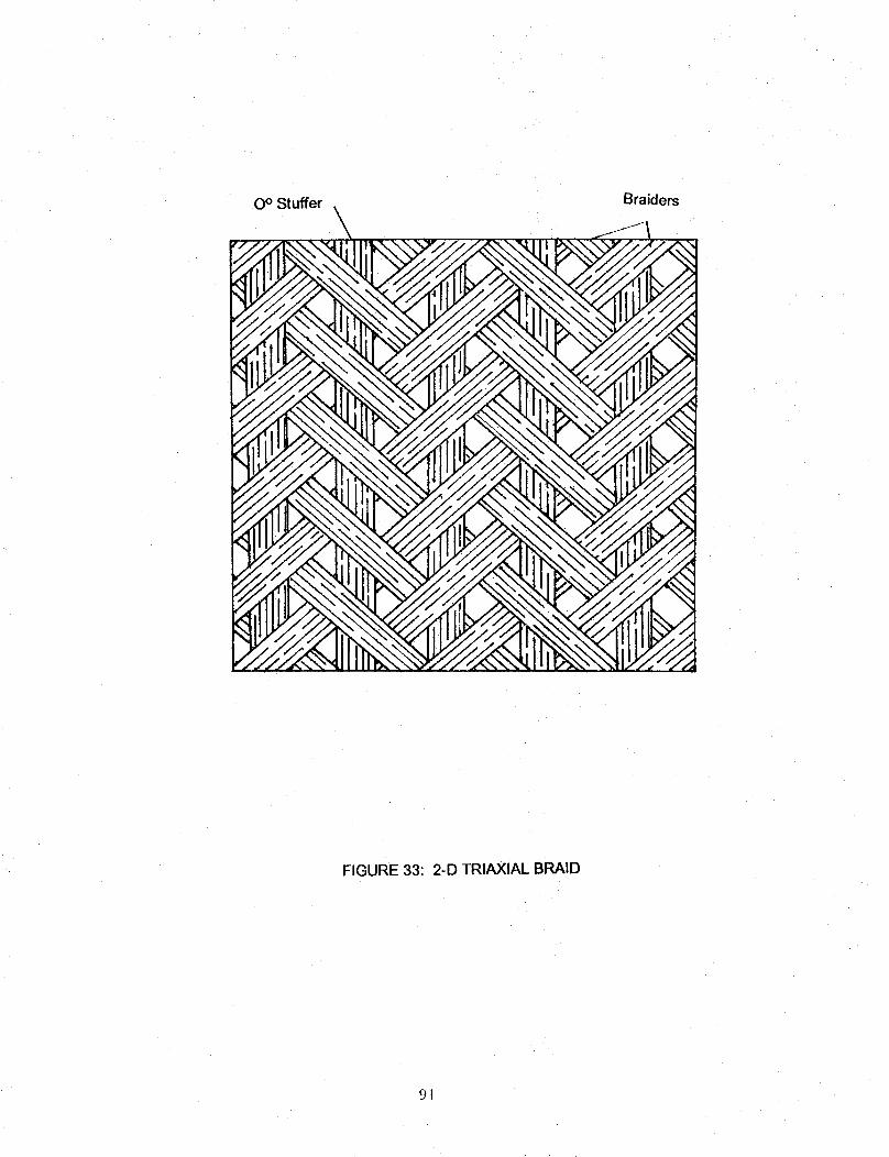
0 ° Stuffer Braiders
FIGURE 33: 2-D TRIAXlAL BRAID
9]
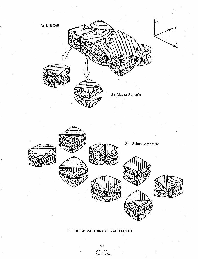
(A) Unit Cell Y
Mas e IC
(B) t r Su ells
(C) Subcell Assembly
FIGURE 34: 2-D TRIAXlAL BRAID MODEL
92

Braider Tow Stuffer Tow
Longitudinal Cross-Section (20x)
Braider Tow Stuffer Tow
• t ,:,r_ • _._i _,_ "';_
Transverse Cross-Section (20x)
FIGURE 35: PHOTOMICROGRAPHS OF TRIAXlAL BRAID
93
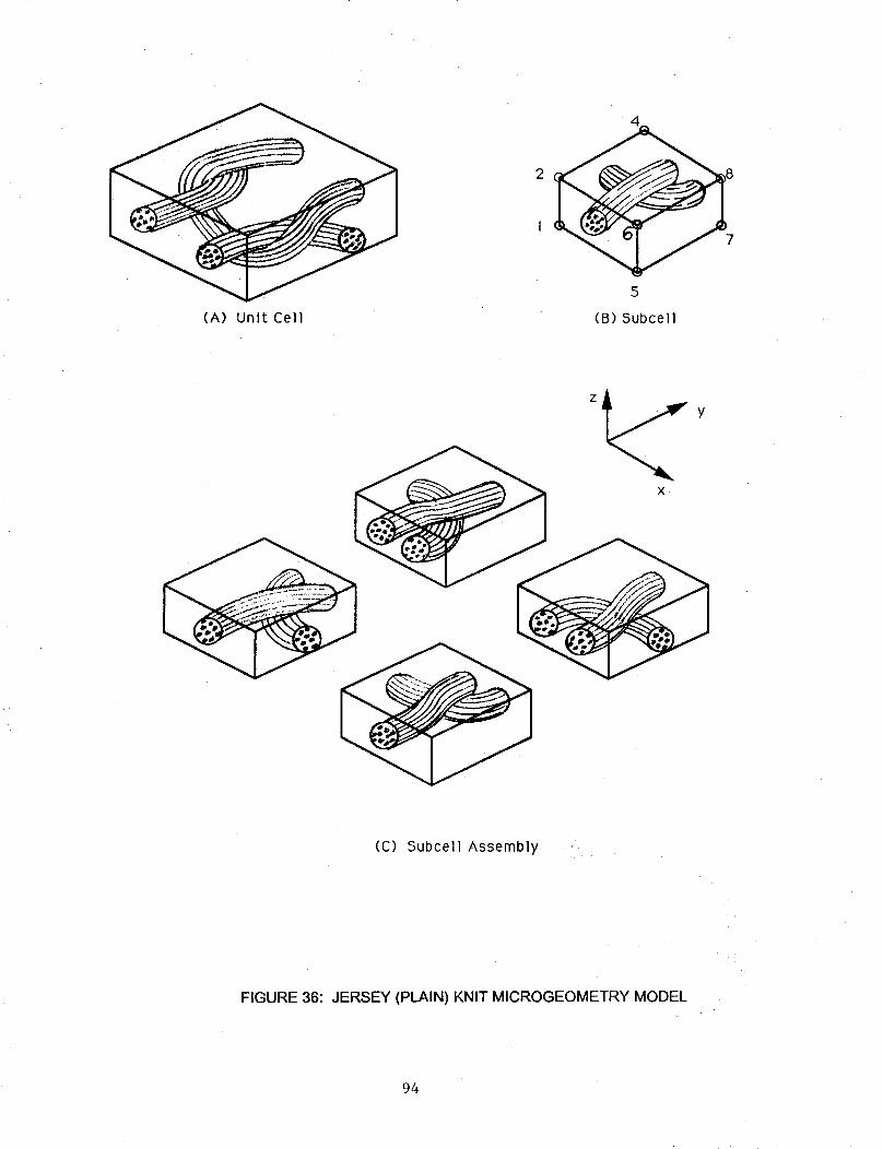
(A) Unit Cell (B) Subcell
(C) Subcell Assembly
FIGURE 36: JERSEY (PLAIN) KNIT MICROGEOMETRY MODEL
94

E,G
(msi)
4 I_
3 _
I
0
Y
A/2
\\\\\\
j- Ex
JJ
_._ Ez _ _._..__...." 2
Gxy
1 1 1 o.2 .4 .6 ,8 1 0
P
AI4B
FIGURE 37: EFFECT OF PRESTRAIN ON JERSEY KNIT COMPOSITE STIFFNESS
95
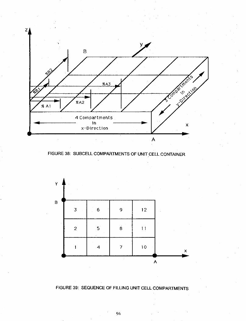
Z
B
Y
%AI
4 Compartmentsin
x-DirectionIlI'--
A
X
FIGURE 38: SUBCELL COMPARTMENTS OF UNIT CELL CONTAINER
3
2
4
9
8
7
12
11
10
A
×
FIGURE 39: SEQUENCE OF FILLING UNIT CELL COMPARTMENTS
96
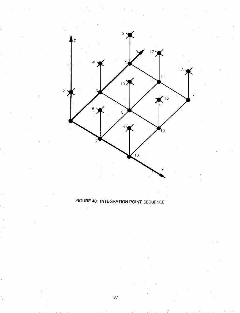
2
4 5
10
8
13
FIGURE 40: INTEGRATION POINT SEQUENCE
97
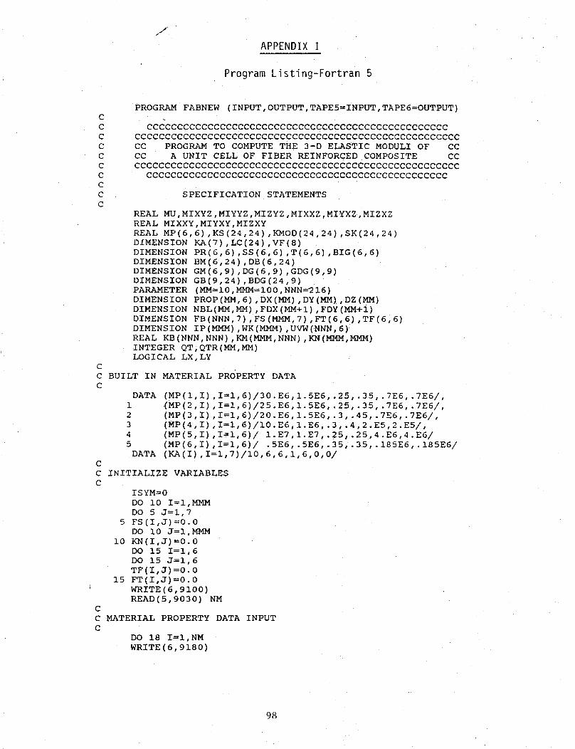
/./
APPENDIX I
Program Listing-Fortran 5
C
C
C
C
C
C
C
C
C
C
PROGRAM FABNEW (INPUT,OUTPUT,TAPEL=INPUT,TAPE6=OUTPUT)
CCCCCCCCCCCCCCCCCCCCCCCCCCCCCCCCCCCCCCCCCCCCCCCCCC
CCCCCCCCCCCCCCCCCCCCCCCCCCCCCCCCCCCCCCCCCCCCCCCCCCCCCC
CC PROGRAM TO COMPUTE THE 3-D ELASTIC MODULI OF CC
CC A UNIT CELL OF FIBER REINFORCED COMPOSITE CC
CCCCCCCCCCCCCCCCCCCCCCCCCCCCCCCCCCCCCCCCCCCCCCCCCCCCCC
CCCCCCCCCCCCCCCCCCCCCCCCCCCCCCCCCCCCCCCCCCCCCCCCCC
SPECIFICATION STATEMENTS
REAL MU,MIXYZ,MIYYZ,MIZYZ,MIXXZ,MIYXZ,MIZXZ
REAL MIXXY,MIYXY,MIZXY
REAL MP(6,6),KS(24,24) ,KMOD(24,24),SK(24,24)DIMENSION KA(7),LC(24) ,VF(8)
DIMENSION PR(6,6),SS(6,6) ,T(6,6),BIG(6,6)
DIMENSION BM(6,24),DB(6,24)
DIMENSION GM(6,9),DG(6,9) ,GDG(9,9)DIMENSION GB[9,24),BDG(24,9)
PARAMETER (MM=I0,MMM=I00,NNN='216)
DIMENSION PROP(MM,6),DX(M_4),DY(MM),DZ(MM)
DIMENSION NBL(MM,MM),FDX(MM+I),FDY(MM+I)
DIMENSION FB(NNN,7),FS(MMM,7),FT(6,6),TF(6,6)
DIMENSION IP(MMM),WK(M/_M),UVW(NNN,6)
REAL KB(NNN,NNN),KM(MMM,NNN),KN(MM_,MM_)
INTEGER QT,QTR(MM,MM)
LOGICAL LX,LY
BUILT IN MATERIAL PROPERTY DATA
DATA
1
2
3
4
5
DATA
C
(MP(I,I),I=I,6)/30.E6,1.5E6,.25,.35,.7E6,.7E6/,
(MP(2,I),I=I,6)/25.E6,1.5E6,.25,.35,.7E6,.7E6/,
(MP(3,I),I=I,6)/20.E6,1.5E6,.3, .45,.7E6,.7E6/,
(MP(4,I),I=I,6)/10.E6,I.E6,.3,.4,2.E5,2.E5/,
(MP(5,I),I=l,6)/ I.E7,I.E7,.25,.25,4.E6,4.E6/
(MP(6,I),I=I,6)/ .5E6,.LE6,.35,.35,.IS5E6,.185E6/
(IZ,A(I),I=l,7)/lO,6,6,1,6,0,O/
C INITIALIZE VARIABLES
C
ISYM=O
DO i0 I=I,MMM
DO 5 J=l,7
5 FS(I,J)=O.0
DO i0 J=I,MMM
i0 KN(I,J)=O.O
DO 15 I=I,6
DO 15 J=l,6
TF(I,J)=O.O
15 FT(I,J)=O.0
WRITE(6,9100)
READ(5,9030) NMC
C MATERIAL PROPERTY DATA INPUT
C
DO 18 I=I,NM
WRITE(6,9180)
98
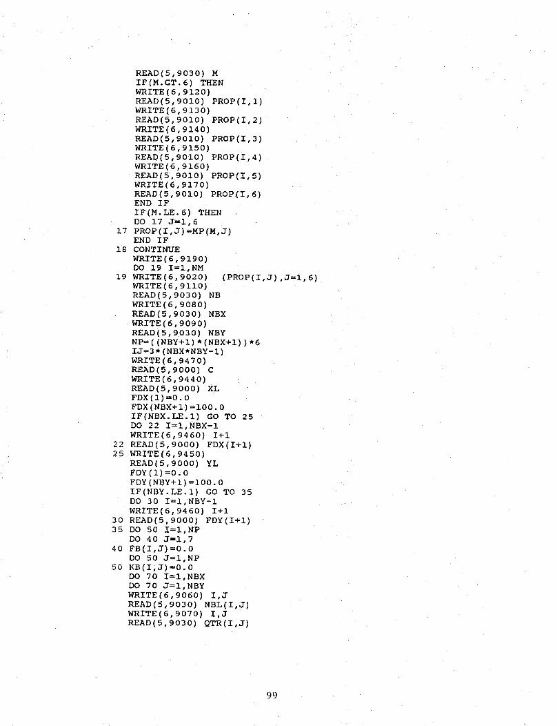
READ (5,9030) M
IF(M.GT. 6) THEN
WRITE (6,9120)
READ (5,9010) PROP (I, i)
WRITE (6,9130)
READ (5,9010) PROP(I, 2)
WRITE (6,9140)
READ(5,9010) PROP(I, 3)
WRITE (6,9150)
READ(5,9010) PROP(I, 4)
WRITE (6,9160)
READ(5,9010) PROP(I, 5)WRITE (6,9170)
READ (5,9010) PROP(I, 6)END IF
IF(M.LE.6) THEN
DO 17 J=l, 6
17 PROP (I, J) =MP (M, J)END IF
18 CONTINUE
WRITE (6,9190)
DO 19 I=I,NM
19 WRITE (6,9020)
WRITE (6,9110)
READ (5,9030)
WRITE (6,9080)
READ(5,9030) NBX
WRITE (6,9090)
READ (5,9030) NBY
NP= ((NBY+I) * (NBX+I)) *6
IJ=3* (NBX*NBY-I)
WRITE (6,9470)
READ(5,9000) C
WRITE(6,9440)
READ(5,9000) XL
FDX (i) =0.0
FDX (NBX+I) =I00.0IF(NBX.LE.I) GO TO 25
DO 22 I=I,NBX-I
WRITE (6,9460) I+l
22 READ(5,9000) FDXII+I)
25 WRITE (6,9450)
READ (5,9000) YL
FDY (i] =0.0
FDY (NBY+I) =i00.0
IF(NBY.LE. i) GO TO 35
DO 30 I=I,NBY-I
WRITE (6,9460) I+l
30 READ(5,9000) FDY(I+I)
35 DO 50 I=I,NP
DO 40 J=l,7
40 FB(I,J) =0.0
DO 50 J=I,NP
50 KB(I,J)=0.0
DO 70 I=I,NBX
DO 70 J=I,NBY
WRITE (6,9060) I,J
READ (5,9030) NBL(I, J)
WRITE (6,9070) I,J
READ(5,9030) QTR(I, J)
(PROP(I,J),J=l,6)
NB
99
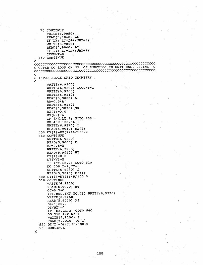
70 CONTINUE
WRITE(6,9050)
READ (5,9040) LX
IF(LX) IJ=IJ+(NBY+I)
WRITE (6,9055)
READ(5,9040) LY
IF(LY) IJ=IJ+(NBX+I)ICOUNT=0
35O CONTINUE
CCCCCCCCCCCCCCCCCCCCCCCCCCCCCCCCCCCCCCCCCCCCCCCCCCCCCCCCCC
C OUTER DO LOOP ON NO. OF SUBCELLS IN UNIT CELL BEGINS C
CCCCCCCCCCCCCCCCCCCCCCCCCCCCCCCCCCCCCCCCCCCCCCCCCCCCCCCCC
C
C
C
INPUT BLOCK GRID GEOMETRY
WRITE(6,9300]
WRITE(6,9200)
WRITE(6,9300)
WRITE(6,9210)
READ(5,9000) AAA=0.5*A
WRITE(6,9240)
READ(5,9030) NX
DX(i) =0.0
DX(NX)=A
IF (NX.LE.2) GOTO 460
DO 450 I=2,NX-I
WRITE(6,9270) I
READ(5,9010) DX(I)
450 DX(I)=DX(I)*A/100.0460 CONTINUE
WRITE(6,9220)
READ(5,9000) BBB=0.5*B
WRITE(6,9250)
READ(5,9030) NY
DY(1) =0.0
DY (NY )=B
IF (NY.LE.2) GOTO 510
DO 500 I=2,NY-I
WRITE(6,9280) I
READ(5,9010) DY(I)
500 DY(I)=DY(I)*B/100.0
510 CONTINUE
WRITE(6,9230)
READ(5,9000) HTCC=0.5*C
IF(.NOT. (HT.EQ.C))
WRITE (6,9260)
READ(5,9030) NZ
DZ(1)=0.0DZ (NZ)=CIF (NZ.LE.2) GOTO 560
DO 550 I=2,NZ-I
WRITE(6,9290) I
READ(5,9010) DZ(I)
550 DZ(I)=DZ(I)*C/100.0
56O CONTINUE
ICOUNT+I
WRITE(6,9330)
100

C GENERAL MATERIALS INFORMATION FOR THE SUBCELL
C
WRITE(6,9310) ICOUNT+I
READC5,9030) NMATMCOUNT=O
DO 570 I=I,24
DO 570 J=1,24
570 KS(I,J)=O-ODO 580 I=i,24
DO 580 J=l,9
580 BDG (I, J) =0-0DO 590 I=i,9
DO 590 J=l,9
590 GDG [I,J)=0.0CCCCCCCCCCCCCCCCCCCCCCCCCCCCCCCCCCCCCCCCCCCCCCCCCCCCCCCCC
C INNER DO LOOP ON MATLS. WITHIN SUBCELL BEGINS HERE C
CCCCCCCCCCCCCCCCCCCCCCCCCCCCCCCCCCCCCCCCCCCCCCCCCCCCCCCCC
600 WRITE(6,9320)
READ(5,9030) MN
CC INPUT 8 MATL. VOL. FRACTIONS AT EACH INTEGRATION POINT
C
8OO
85O
860
DO 2000 I=I,NX
DO 2000 J=I,NY
DO 2000 K=I,NZ
DO 800 LL=I,8
VF (LL) =0.0WRITE (6,9480)
READ(5,9000) A1
WRITE (6,9490)
READ (5,9000) A2
WRITE (6,9420) I,J,K
READ(5,9030) L
IF((L.LT.0) .OR. (L.GT.8))
WRITE (6,9430) L
READ (5,9000) VF(L)GO TO 850
CONTINUE
IF(I.EQ.NX) THENXP=O. 0
ELSE
XP= CDX (I+l) -DX (I))/2.0
END IF
IF(I.EQ. i) THENXM=0.0
ELSE
XM= (DX (I) -DX (I-l))/2.0
END I F
IF (J. EQ. NY) THEN
YP=0.0
ELSE
YP= (DY (J+l) -DY (J) ]/2.0
END IF
IF(J.EQ.I) THENYM=O. 0
ELSE
YM= (DY (J)-DY (J-l))/2.0
END IF
IF (K.EQ.NZ) THEN
ZP=0.0
GO TO 860
101

ELSEZP=(DZ(K+l) -DZ(K))/2.0ENDIFIF(K.EQ. i) THENZM=0.0ELSEZM=(DZ(K) -DZ(K-l))/2.0ENDIFVI=VF(I) *XP*YP*ZPV2=VF(2) *XP*YP*ZMV3=VF(3) *XP*YM*ZPV4=VF(4) *XP*YM*ZMV5=VF(5) *XM*YP*ZPV6=VF(6) *XM*YP*ZMV7=VF(7) *XM*YM*ZPVS=VF(8) *XM*YM*ZMVOL=VI+V2+V3+V4+VS+V6+V7+V8
GETTHE STRAINTRANSFORMATIONMATRIX(T)
SI=SIND(AI)S2=SIND(A2)CI=COSD(AI)C2=COSD(A2)SIS=SI*SI$2S=$2-$2ClS=CI*CI
C2S=C2"C2
SCI=SI*CI
SC2=$2"C2
T(I,I)=CIS*C2S
T(I, 2) =SIS*C2S
T(I,3)=$2S
T (i, 4) =SCI*C2S
T(I, 5) =SI*SC2
T (I, 6) =CI*SC2
T(2,1)=SIS
T(2,2) =CIS
T(2,3)=0.0
T(2,4)=-SCI
T(2,5]=0.0
T(2,6)=0.0
T(3,1]=ClS*S2S
T(3,2]=SIS*$2S
T(3,3)=C2S
T (3,4) =SCl*S2S
T (3 , 5) =-SI*SC2
T (3 , 6) =-CI*SC2
T(4,1)=-2.0"SCI*C2
T(4,2)=-T(4,1)
T(4,3)=0.0
T(4,4) = (CIS-SIS) *C2
T (4,5) =CI*S2
T(4,6) =-SI*$2
T 15, i) =2.0*SCI*S2
TI5,2)=-T(5,1)
T(5,3)=0.0
T (5,4) =- (CIS-SIS) *$2
T (5,5) =CI*C2
T(5,6) =-SI*C2
]_02

C
C GET
C
ii00
T(6,1)=-2.0"CIS*SC2
T(6,2)=-2.0"SIS*SC2
T(6,3)=2.0"SC2T(6,4)=-SCI*SC2"2.0
T(6,5)=SI*(C2S-$2S)
T(6,6)=CI*(C2S-$2S)
STRESS-STRAIN MATRIX (SS) IN MATL. COORD. SYSTEM
DO ll00 II=l,6
DO Ii00 JJ=l,6
SS(II,JJ)=0.0MC=MN
MU=PROP(MC,4)
R=PROP(MC,3)*PROP(MC,3)*PROP(MC,2)/PROP(MC, I)
D=(I.0+MU)*(I.0-MU-2.0*R)
IF(D.LE.0.0) D=I.0
SS(I,I)=PROP(MC,I)*(I.0-MU*MU)/D
SS(I,2)=PROP(MC,2)*PROP(MC,3)*(I-0+MU)/D
SS (1,3)=SS (1,2)
SS (2, I) =SS (i, 2)
SS (2,2) =PROP(MC, 2) * (I. 0-R)/D
SS (2,3) =PROP (MC, 2) * (MU+R)/D
ss(_, 1)=ss(1,3)SS(3,2)=SS(2,3)
SS(3,3)=SS(2,2)
SS (4,4) =PROP(MC, 5)
SS (5,5) =PROP (MC, 6)
SS (6,6) =PROP (MC, 5)
C
C GET
C
1150
1200
1225
1250
1300
1350
C
STRESS-STRAIN MATRIX (SS) IN COORDS. OF THE
DO 1200 II=l,6
DO 1200 JJ=l,6
SUM=0.0
DO 1150 KK=I,6
SUM=SUM+SS(II,KK)*T(KK,JJ)
PR(II,JJ)=SUMDO 1225 II=l,3
DO 1225 JJ=4,6
T(II,JJ)=2.0*T(II,JJ)
T[JJ,II)=0.5*T(JJ,II)CALL MATOPS(KA,T,DET,DDDD)
DO 1300 II=l,6
DO 1300 JJ=l,6
SUM=0 •0DO 1250 KK=I,6
SUM=SUM+T (I I, KK) * PR (KK, JJ )
BIG(II,JJ)=SUM*VOL
CONTINUE
SUBCELL GEOMETRY CALCULATIONS
1400
1500
DO 1400 II=l,6
DO 1400 JJ=l,9
GM(II,JJ)=0.0DO 1500 II=l,6
DO 1500 JJ=l,24
BM (II, JJ) =0.0
SUBCELL
103

CC
C
FORM 8 NODE FINITE ELEMENT STIFFNESS MATRIX FOR
X=DX (I)-AAY=DY (J) -BB
Z=DZ (K)-CCXl =- (0. 125/AA) * (i. O-Y/BB)
YI=-(0. 125/BB) * (I. 0-X/AA)
Z1 =-(0.125/cC)* (I.0-X/AA)
X2=- (0. 125/AA) * (I. 0-Y/BB)
Y2 =- (0. 125/BB) * (1.0-X/AA)
Z2=+ (0. 125/CC) * (I. O-X/AA)
X3=- (0. 125/AA) * (i. 0+Y/BB)
Y3=+ (0. 125/BB) * (i. 0-X/AA)
z3=- (0. 125/cc) *(I.0-X/AA)X4=-(0.125/AA)*(I.0+Y/BB)
Y4=+ (0. 125/BB) * (i. 0-X/AA)
Z4=+ (0. 125/CC) * (I. 0-X/AA)
X5=+ (0. 125/AA) * (i. 0-Y/BB)
Y5=- (0. 125/BB) * (i. 0+X/AA)
Z5=- (0. 125/CC) * (i. O+X/AA)
X6=+ (0. 125/AA) * (i. 0-Y/BB)
Y6=- (0. 125/BB) * (1.0+X/AA)
Z6=+ (0. 125/CC) * (i. 0+X/AA)
X7=+ (0. 125/AA) * (i. 0+Y/BB)
Y7=+ (0. 125/BB) * (I. 0+X/AA)
Z7 =- (0. 125/CC) * (i. 0+X/AA)
X8=+ (0. 125/AA) * (i. 0+Y/BB)
Y8=+ (0. 125/BB) * (i. 0+X/AA)
Z8=+ (0. 125/CC) * (I. 0+X/AA)
XX=-2.0*X/(AA*AA)YY=-2.0*Y/(BB*BB)
ZZ=-2.0*Z/(CC*CC)GM(I, I}=XX
GM(2,5)=YY
GM(3,9} =ZZ
GM(4,2 =XX
GM (4,4 =YY
GM(5,6 =YY
GM(5,8 =ZZ
GM(6,3 =XX
GM(6,7 =ZZ
BM(I, 1 =XI
BM(2,2)=YI
BM(3,3)=ZI
BM(I,4}=X2
BM(2,51 =Y2
BM(3,6)=Z2
BM(I,7)=X3
BM(2,8)=Y3
BM(3,9)=Z3
BM(I, i0) =X4
BM(2, Ii) =Y4
BM(3,12) =Z4
BM(I, 13)=X5
BM(2,14) =Y5
BM(3 , 15) =Z5
BM(I, 16) =X6
BM(2,17) =Y6
BM(3,18) =Z6
* (i.o-z/cc)* (l.O-Z/CC)* (i. 0-Y/BB)
* (i.O+Z/CC)* (i.o+z/cc)* (i. O-Y/BB)
* (i.o-z/cc)* (l.O-Z/CC)* (I. 0+Y/BB)
* (I.o+Z/CC)* (i.o+z/cc)* (i. 0+Y/BB)
* (I. o-z/cc)* (i. o-z/cc)* (I. 0-Y/BB)
* (I. 0+Z/CC)* (i. O+Z/CC)* (i. 0-Y/BB)
* (I. o-z/cc)* (i. o-z/cc)* (i. 0+Y/BB)
* (i. o+z/cc)* (l.O+Z/CC)* ( I. 0+Y/BB)
SUBCELL
104
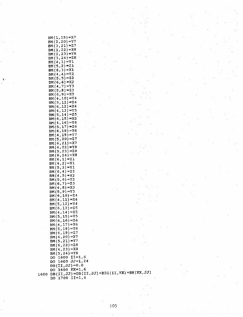
1600
BM(I,19)=X7
BM(2 20)=Y7
BM(3 21)=Z7
BM(I 22)=X8
BM(2 23) =Y8
BM(3 24) =Z8
BM(4 1)=Yl
BM(5 2)=ZI
BM(6 3)=XI
BM(4 4)=Y2
BM(5,5)=Z2
BM(6,6) =X2
BM(4,7] =Y3
BM(5,8]=Z3
BM(6,9]=X3
BM(4,10)=Y4
BM(5,11)=Z4
BM(6,12)=X4
BM(4,13)=Y5
BM(5,14)=Z5
BM(6,15)=X5
BM(4,16)=Y6
BM(5,17)=Z6
BM(6,18)=X6
BM(4,19) =Y7
BM(5,20)=Z7
BM(6,21)=X7BM [4,22 ) =Y8
BM(5,23) =Z8
BM(6,24)=X8
BM(6,1)=Z1
BM(4,2)=XI
BM(5,3)=YI
BM(6,4)=Z2
BM(4,5)=X2
BM(5,6)=Y2
BM(6,7)=Z3
BM(4,8]=X3
BM(5,9)=YS
BM(6,10)=Z4
BM(4,11)=X4
BM(5 12)=Y4
BM(6 13)=Z5
BM(4 14)=X5
BM(5 15)=Y5
BM(6 16) =Z6
BM(4 17) =X6
BM(5 18) =Y6
BM(6 19)=Z7
BM(4.20)=X7
BM(5 21)=Y7
BM(6,.22)=Z8
BM(4.23)=X8
BM(5,24)=Y8
DO 1600 II=l,6
DO 1600 JJ=l,24
DB(II,JJ)=O.0
DO 1600 KK=I,6
DB(II,JJ)=DB(II,JJ)+BIG(II,KK)*BM(KK,JJ)
DO 1700 II=l,6
105
1700
1750
1800
1900
2000
2020
2030
2040
C
C PUT
C
2050
2100
2200
DG(II,I)=XX*BIG(II,I)
DG(II,2)=XX*BIG(II,4)
DG(II,3)=XX*BIG(II,6)
DG(II,4)=YY*BIG(II,4)
DG(II,5)=YY*BIG(II,2)
DG(II,6)=YY*BIG(II,5)
DG(II,7)=ZZ*BIG(II,6)
DG(II,8)=ZZ*BIG(II,5)
DG(II,9)=ZZ*BIG(II,3)DO 1750 II=l,9
DO 1750 JJ=l,9DO 1750 KK=I,6
GDG(II,JJ)=GDG(II,JJ)+GM(KK,II)*DG(KK,JJ)
DO 1800 II=i,24
DO 1800 JJ=l,9
DO 1800 K_=I,6
BDG(II,JJ)=BDG(II,JJ)+BM(KK,II)*DG(KK,JJ)
DO 1900 II=i,24
DO 1900 JJ=l,24
DO 1900 KK=I,6
KS(!I,JJ)=KS(II,JJ)+BM(KK, II)*DB(ICK,JJ)CONTINUE
MCOUNT=MCOUNT+I
IF(MCOUNT.LT.NMAT) GO TO 600
CALL INV(GDG)
DO 2020 I=i,9
DO 2020 J=i,24
GB(I,J)=0.0DO 2020 K=I,9
GB(I,J)=GB(I,J)+GDG(I,K)*BDG(J,K)
DO 2030 I=I,24
DO 2030 J=i,24
KMOD(I,J)=0.0
DO 2030 K=I,9
KMOD (I, J)=KMOD (I, J) +BDG (I, K) *GB (K, J)
DO 2040 I=i,24
DO 2040 J=i,24
KS (I,J) =KS (I,J) -KMOD(I,J)
SMALL STIF. MATRIX (KS) INTO BIG STIF. MATRIX (KB)
ICOUNT=ICOUNT+I
DO 2400 I=I,NBX
DO 2400 J=I,NBY
QT=QTR(I,J)
NK=NBL(I,J)
IF(.NOT. (NK.EQ.ICOUNT)) GO TO
IF(QT.LT.0) GO TO 2400
DO 2050 II=i,24
DO 2050 JJ=l,24
SK(II,JJ)=KS(II,JJ)
IF(QT.EQ.0) GO TO 2100
CALL TRNS (QT, SK)
LC (i) = ((NBY+I) * (I-l) +J-l) "6+1
LC (13) =LC (1) + (NBY+I) *6
DO 2200 K=2,12
LC(K)=LC(K-I)+I
LC(K+I2)=LC(K+II)+I
DO 2300 II=i,24
DO 2300 JJ=l,24
2400
106
III=LC(II)JJJ=LC(JJ)
2300 KB(III,JJJ)=KB(III,JJJ)+SK(II,JJ)2400 CONTINUE
IF(ICOUNT.LT.NB) GO TO 350GO TO 2460
2440 ISYM=I
DO 2445 I=l,IJ
DO 2445 J=l,IJ
2445 KN(I,J)=0.O
DO 2447 I=l,IJ
2447 KN[I,I)=I.0
IF(LX) IJ=IJ-2*NBY+I
IF[LY) IJ=IJ-2*NBX+I
DO 2450 I=I,NP
DO 2450 J=l,6
2450 FB(I,J)=O.0
2460 CONTINUE
CALC. DISP. VECTORS FOR 6 HOMOGENEOUS UNIT STRAIN CASES
2500
2525
C
C USE
C
2850
2900
C
C USE
C
2950
DO 2500 I=I,NBX+I
DO 2500 J=IoNBY+I
K=((I-I)*(NBY+I)+(J-I))*6+I
FB(K,I)=FDX(I)*XL/100.0
FB(K+3,1)=FB(K,I)
FB(K+I,2)=FDY(J)*YL/100.O
FB(K+4,2)=FB(K+I,2)
FB(K+5,3)=C
FB(K,4)=FB(K+I,2)
FB(K+3,4)=FB(K,4)
FB(K+4,5)=C
FB(K+3,6)=C
DO 2525 I=I,NP
DO 2525 J=l,6
UXFW(I,J)=FB(I,J)
FORCE B.C.S TO ELIMINATE INTERNAL SURFACE FORCES
IN=0
IF((NBX.LE.I).OR.(NBY.LE.I))GO TO 2950
DO 2900 I=2,NBX
DO 2900 J=2,NBY
L=[(I-I)*(NBY+I)+(J-I))*6
DO 2850 K=I,NP
KM(IN+I,K)=KB(L+I,K)+KB(L+4,K)
KM(IN+2,K)=KB(L+2,K)+KB(L+5,K)
KM(IN+3,K)=KB(L+3,K)+KB(L+6,K)IN=IN+3
CONTINUE
FORCE B.C.S TO ELIMINATE FORCE AT SIDE NODES
IF(NBX.LE.I) GO TO 3150
DO 3100 I=2,NBX
L=6*(I-1)*(NBY+I)LL=L+NBY*6
IF(LY) GO TO 3050DO 3000 K=I,NP
KM(IN+I,K)=KB(L+I,K)+KB(L+4,K)+KB(LL+I,K)+KB(LL+4,K)
107
3000
3050
3075
3O8O
3085
309031003150
3200
3250
3275
3280
3285
329033003305
3310
3311
3312
DO3075KM(IN+IKM(IN+2KM(IN+3KM(IN+4IN=IN+4
KM[IN+2,K)=KB(L+2,K)+KB(L+5,K)+KB(LL+2,K)+KB(LL+5,K)KM(IN+3,K)=KB(L+3,K)+KB(L+6,K)+KB(LL+H,K)+KB(LL+6,K)IN=IN+3GO TO 3100
CONTINUE
IF(ISYM.EQ.I) GO TO 3080
K=I,NP
,K) =KB(L+I,K) +KB(L+4, K)
,K) =KB (L+3, K) +KB (L+6, K)
,K) =KB (LL+I, K) +KB (LL+4, K)
,K)=KB(LL+3,K)+KB(LL+6,K)
GO TO 3090
CONTINUE
DO 3085 K=I,NP
KM(IN+I,K)=KB(L+2,K)+KB(L+5,K)
KM(IN+2,K)=KB(LL+2,K)+KB(LL+5,K)INffiIN+2
CONTINUE
CONTINUE
IF(NBY.LE.I) GO TO 3305DO 3300 J=2,NBY
L=6*(J-I)
LL=L+NBX*(NBY+I)*6
IF(LX) GO TO 3250DO 3200 K=I,NP
KM(IN+I,K)=KB(L+I,K)+KB(L+4,K)+KB(LL+I,K)+KB(LL+4,K)
KM(IN+2,K)=KB(L+2,K)+KB(L+5,K)+KB(LL+2,K)+KB(LL+5,K)
KM(IN+3,K)=KB(L+3,K)+KB(L+6,K)+KB(LL+3,K)+KB(LL+6,K)IN=IN+3
GO TO 3300
CONTINUE
IFIISYM.EQ.I) GO TO 3280
DO 3275 K=I,NP
KM(IN+I,K)=KB(L+2,K)+KB(L+5,K)
KM(IN+2,K)=KB(L+3,K)+KB(L+6,K)
KM(IN+3,K)=KB(LL+2,K)+KB(LL+5,K)
KM(IN+4,K)=KB(LL+3,K)+KB(LL+6,K)IN=IN+4
GO TO 3290
CONTINUE
DO 3285 K=I,NP
KM(IN+I,K)=KB(L+I,K)+KB(L+4,K)
KM(IN+2,K)=KB(LL+I,K)+KB(LL+4,K)
IN=IN+2
CONTINUE
CONTINUE
CONTINUE
IF(.NOT.LY) GO TO 3315L=6*NBY
LL=L+6*NBX*(NBY+I)
IF(ISYM.EQ.1) GO TO 3311
DO 3310 K=I,NP
KM(IN+I,K)=KB(L+I,K)+KB(L+4,K)+KB(LL+I,K)+KB(LL+4,K)
KM(IN+2,K)=KB(L+3,K)+KB(L+6,K)+KB(LL+3,K)+KB(LL+6,K)IN=IN+2
GO TO 3314
CONTINUE
DO 3312 K=I,NP
KM(IN+I,K)=KB(L+2,K)+KB(L+5,K)+KB(LL+2,K)+KB(LL+5,K)
108
33143315
3320
3321
3322
33243325
9085
3330
3335
33403345
CC USEC
3350
33753400
3425
3430
IN=IN+ICONTINUECONTINUEIF(.NOT.LX) GOTO 3325L=6*NBX*(NBY+I)LL=L+6*NBYIF(ISYM.EQ.I) GOTO 3321DO 3320 K=I,NPKM(IN+I,K)=KB(L+2,K)+KB(L+5,K)+KB(LL+2,K)+KB(LL+5,K)KM(IN+2,K)=KB(L+3,K)+KB(L+6,K)+KB(LL+3,K)+KB(LL+6,K)IN=IN+2GOTO 3324CONTINUEDO3322 K=I,NPKM(IN+I,K)=KB(L+I,K)+KB(L+4,K)+KB(LL+I,K)+KB(LL+4,K)IN=IN+ICONTINUECONTINUEIF(IJ.LT.I) GOTO 3345FORMAT(IH,6F12.0)DO3330 I=l,IJDO3330 J=l,7FS(I,J) =0.0
DO 3340 I=i,6
DO 3335 J=I,IN
DO 3335 K=I,NP
FS (J, 7) =FS (J, 7) +KM (J, K) *UVW (K, I)
DO 3340 J=l,IJ
FS (J, I) =FS (J, 7)
FS(J,7)=0.O
CONTINUE
DISPLACEMENT B.C.S TO ELIMINATE DISPLACEMENTS
INN=IN
IN=0
IF(IJ.LT.I) GO TO 3575
IF((NBX.LE.I).OR. (NBY.LE.I)) GO TO 3400
DO 3375 I=2,NBX
DO 3375 J=2,NBY
L=((I-I)*(NBY+I)+(J-I))*6DO 3350 K=I,INN
KN(K, IN+I)=KM(K,L+I)+KM(K,L+4)
KN(K,IN+2)=KM(K,L+2)+KM(K,L+5)
KN(K,IN+3)=KM(K,L+3)+KM(K,L+6)
IN=IN+3
CONTINUE
CONTINUE
IF(NBX.LE.I) GO TO 3475
DO 3450 I=2,NBX
L=6*(I-I)*(NBY+I)LL=NBY*6+L
IF(LY) GO TO 3430DO 3425 K=I,INN
KN(K,IN+I]=KM(K,L+I)+KM(K,L+4)+KM(K,LL+I)+KM(K,LL+4)
KN(K,IN+2]=KM(K,L+2)+KM(K,L+5)+KM(K, LL+2)+KM(K,LL+5)
KN(K,IN+3)=KM(K,L+3)+KM(K,L+6)+KM(K,LL+3)+KM(K,LL+6)
IN=IN+3GO TO 3450
CONTINUE
109
3440
3445
3447
344934503475
3480
3490
3495
3496
3497
349935003510
3520
3530
3535
35403550
IF(ISYM.EQ.I) GOTO 3445DO3440 K=I,INNKN(K,IN+I)=KM(K,L+I)+KM(K,L+4)KN(K,IN+2)=KM(K,L+3)+KM(K,L+6)KN(K,IN+3)=KM(K,LL+I)+KM(K,LL+4)KN(K,IN+4)=KM(K,LL+3)+KM(K,LL+6)IN=IN+4GOTO 3449CONTINUEDO 3447 K=I,INNKN(K,IN+I)=KM(K,L+2)+KM(K,L+5)KN(K,IN+2)=KIM(K,LL+2)+KM(K,LL+5)IN=IN+2CONTINUECONTINUECONTINUEIF(NBY.LE.I) GOTO 3510DO3500 J=2,NBYL=6* (J-l)LL=6*NBX*(NBY+I)+LIF(LX) GOTO 3490DO 3480 K=I,INNKN(K,IN+I)=KM(K,L+I)+KM(K,L+4)+KM(K,LL+I)+KM(K,LL+4)KN(K,IN+2)=k94(K,L+2)+KM(K,L+5)+KM(K,LL+2)+KM(K,LL+5)KN(K,IN+3)=KM(K,L+3)+KM(K,L+6)+KM(K,LL+3)+KM(K,LL+6)IN=IN+3GOTO 3500CONTINUEIF(ISYM.EQ.I) GOTO 3496DO3495 K=I,INNKN(K,IN+I)=KM(K,L+2)+KM(K,L+5)KN(K,IN+2)=KM(K,L+3)+KM(K,L+6)KN(K,IN÷3)=KM(K,LL+2)+KM(K,LL+5)KN(K,IN+4)=KM(K,LL+3)+KM(K,LL+6)IN=IN+4
GO TO 3499
CONTINUE
DO 3497 K=I,INN
KN(K,IN+I)=KM(K,L+I]+KM(K,L+4)
KN(K,IN+2)=KMCK,LL+I)+KM(K, LL+4)IN=IN+2
CONTINUE
CONTINUE
CONTINUE
IFC.NOT.LY) GO TO 3550
L=6*NBY
LL=L+6*NBX*(NBY+I)
IF(ISYM.EQ.I) GO TO 3530
DO 3520 K=I,INN
KN(K, IN+I)=KM(K,L+I)+KM(K,L+4)+KM(K, LL+I)+KM(K, LL+4)
KN(K,IN+2)=KM(K,L+3)+KM(K,L+6)+KM(K,LL+3)+KM(K,LL+6)IN=IN+2
GO TO 3540
CONTINUE
DO 3535 K=I,INN
KN(K,IN+I)=KM(K,L+2)+KM(K,L+5)+KM(K,LL+2)+KM(K,LL+5)
IN=IN+I
CONTINUE
CONTINUE
IF(.NOT.LX) GO TO 3570
110

3560
3565
3566
3569
3570
C
C GET
C
C
C GET
C
3575
3590
3600
3625
3650
3700
3710
3720
L=6*NBX*(NBY+I)LL=L+6*NBY
IF(ISYM.EQ.I) GO TO 3565
DO 3560 K=I,INN
KN(K,IN+I)=KM(K,L+2)+KM(K,L+5)+KM(K,LL+2)+KM(K,LL+5)
KN(K, IN+2)=KM(K,L+3)+KM(K,L+6)+KM(K,LL+3)+KM(K,LL+6)IN=IN+2
GO TO 3569
CONTINUE
DO 3566 K=I,INN
KN(K,IN+I)=KM(K,L+I)+KM(K,L+4)+KM(K,LL+I)+KM(K,LL+4)IN=IN+I
CONTINUE
CONTINUE
UNCONSTRAINED DISPLACEMENTS FOR 6 UNIT STRAIN CASES
IZ=0
CALL GELIM(MMM,IJ,KN,7,FS,IP,IZ,WK,IERR)
A COMPLETE SET OF TOTAL DISPLACEMENTS
IN=0
IF((NBX.LE.I).OR.(NBY.LE.I)) GO TO 3650DO 3625 I=2,NBX
DO 3625 J=2,NBY
LL=(I*NBY+I+J-NBY-2)*6
DO 3600 K=I,3KP=K+3
DO 3600 L=I,6
UVW(LL+K,L)=UVW(LL+K,L)-FS(IN+K,L)
UVW(LL+KP,L)=UVW[LL+KP,L)-FS(IN+K,L)IN=IN+3
CONTINUE
IFINBX.LE.I) GO TO 3750
DO 3740 I=2,NBX
L=6*(I-I)*(NBY+I)LL=L+NBY*6
IF(LY) GO TO 3710
DO 3700 K=I,3
KP=K+3
DO 3700 M=I,6
UVW(L+K,M) =UVW(L+K,M) -FS(IN+K,M)
UVW(L+KP,M) =UVW(L+KP,M) -FS(IN+K,M)
UVW(LL+K,M)=UVW(LL+K,M)-FS(IN+K,M)
UVW(LL+KP,M)=UVW(LL+KP,M)-FS(IN+K,M)IN=IN+3
GO TO 3740
CONTINUE
IF(ISYM.EQ.I) GO TO 3730
DO 3720 M=l,6
UVW (L+I, M) =UVW (L+I, M) -FS (IN+l, M)
UVW[L+3,M)=UVW(L+3,M)-FS(IN+2,M)
UVW[L+4,M)=UVW(L+4,M)-FS(IN+I,M)
UVW(L+6,M)=[YVW(L+6,M)-FS(IN+2,M)
UVW(LL+I,M)=UVW(LL+I,M)-FS(IN+3,M)
UVW[LL+3,M)=UVW(LL+3,M)-FS(IN+4,M)
UVW(LL+4,M)=UVW(LL+4,M)-FS(IN+3,M)
UVW(LL+6,M)=UVW(LL+6,M)-FS(IN+4,M)
IN=IN+4
iii
3730
3735
373737403750
3800
3810
3820
3825
3830
3835
3845
385O
3860
GO TO 3737
CONTINUE
DO 3735 M=I,6
UVW(L+2,M)=UVW(L+2,M)-FS(IN+I,M)
UVW[L+5,M)=UVW(L+5,M)-FS(IN+I,M)
UVW[LL+2,M)=UVW(LL+2,M)-FS(IN+2,M)
UVWCLL+5,M)=UVW(LL+5,M)-FS(IN+2,M)IN=IN+2
CONTINUE
CONTINUE
IF(NBY.LE.I) GO TO 3850
DO 3845 J=2,NBY
L = 6*(J-l)
LL=L+ 6*(NBY+I)*NBX
IF(LX) GO TO 3810
DO 3800 K=I,3KP=K+3
DO 3800 M=I,6
UVW(L+K,M) =UVW(L+K,M) -FS(IN+K,M)
UVW(L+KP,M) =UVW(L+KP,M) -FS(IN+K,M)
UVW(LL÷K,M) =UVW(LL+K,M) -FS(IN+K,M)
UVW(LL+KP,M) =UVWCLL+KP,M ) -FS(IN+K,M)IN=IN+3
GO TO 3845
CONTINUE
IF(ISYM.EQ.I) GO TO 3825
DO 3820 M=I,6
UVW(L+2,M)=UVW(L+2,M)-FS(IN+I,M)
UVW(L+3,M)=UVW(L+3,M)-FS(IN+2,M)
UVW(L+5,M)=UVW(L+5,M)-FS(IN+I,M)
UVW(L+6,M)=UVW(L+6,M)-FS(IN+2,M)
UVW(LL+2,M)=UVW[LL+2,M)-FS(IN+3,M)
UVW(LL+3,M)=UVW(LL+3,M)-FS(IN+4,M)
UVW(LL+5,M)=UVW(LL+5,M)-FS(IN+3,M)
UVW(LL+6,M)=UVW(LL+6,M)-FS(IN+4,M)IN=IN+4
GO TO 3835
CONTINUE
DO 3830 M=I,6
UVW(L+I,M)=UVW(L+I,M)-FS(IN+I,M)
UVW(L+4,M)=UVW(L+4,M)-FS(IN+I,M)
UVW(LL+I,M)=UVW(LL+I,M)-FS(IN+2,M)
UVW(LL+4,M)=UVW(LL+4,M)-FS(IN+2,M)IN=IN+2
CONTINUE
CONTINUE
CONTINUE
IF[.NOT.LY) GO TO 3870L=6*NBY
LL=L+6*NBX*(NBY+I)
IF[ISYM.EQ.I) GO TO 3865
DO 3860 M=l,6
UVW(L+I,M)=UVW(L+I,M)-FS(IN+I,M)
UVW(L+3,M)=UV (L+3,M)-FS(IN+2,M)
UVW(L+4,M)=UVW(L+4,M)-FS(IN+I,M)
UVW(L+6,M)=UVW(L+6,M)-FS(IN+2,M)
UVW(LL+I,M)=UVW(LL+I,M)-FS(IN+I,M)
UVW(LL+3,M)=UVW(LL+3,M)-FS(IN+2,M)
UVW(LL+4,M)=UVW(LL+4,M)-FS(IN+I,M)
UVW(LL+6,M)=UVW(LL+6,M)-FS(IN+2,M)
112
3865
3866
38693870
388O
3885
3886
38893890
CC COMPUTENODALFORCESC
IN=IN+2GOTO 3869CONTINUEDO3866 M=I,6UVW(L+2,M)=UVW(L+2,M)-FS(IN+I,M)
UVW(L+5,M)=UVW(L+5,M)-FS(IN+I,M)
UVW(LL+2,M)=UVW(LL+2,M)-FS(IN+I,M)
UVW(LL+5,M)=UVW(LL+5,M)-FS(IN+I,M)IN=IN+I
CONTINUE
CONTINUE
IF(.NOT.LX) GO TO 3890
L=6*NBX*(NBY+I)LL=L+6*NBY
IF(ISYM.EQ.I) GO TO 3885
DO 3880 M=I,6
UVW{L+2,M)=LrVW(L+2,M)-FS(IN+I,M)
UVW{L+3,M)=UVW(L+3,M)-FS(IN+2,M)
UVW(L+5,M)=UVW(L+5,M)-FS(IN+I,M)
UVW(L+6,M)=UVW(L+6,M)-FS(IN÷2,M)
UVW(LL+2,M)=UVW(LL+2,M)-FS(IN+I,M)
UVW(LL+3,M)=UVW(LL+3,M)-FS(IN+2,M)
UVW(LL+5,M)=UVW(LL+5,M)-FS(IN+I,M)
UVW(LL+6,M)=UVW(LL+6,M)TFS(IN+2,M)IN=IN+2
GO TO 3889
CONTINUE
DO 3886 M=I,6
UVW(L+I,M)=UVW(L+I,M)-FS(IN+I,M)
UVW(L+4,M)=UVW(L+4,M)-FS(IN+I,M)
UVW(LL+I,M)=UVW(LL+I,M)-FS(IN+I,M)
UVW(LL+4,M)=UVW(LL+4,M)-FS(IN+I,M)IN=IN+I
CONTINUE
CONTINUE
IF(NP.LT.1) GO TO 3950
DO 3900 I=I,NP
DO 3900 J=l,6
FB(I,J) =0.0
DO 3900 K=I,NP
FB (I,J) =FB (I, J) +KB(I, K) *UVW (K, J)CONTINUE
3900
3950
C
C COMPUTE SIDE LOADS FOR EACH OF THE 6 UNIT
C
4200
YLC=YL*C
XLC=XL*C
DO 4500 I=I,6
DO 4200 J=I,NBY+I
K=(J-I)*6
FT(Itl)=FT(I,I)+FB(K+I,I)+FB(K+4,I)
FT(4,I)=FT(4,I)+FB(K+2,I)+FB(K+5,I)
FT(6,I)=FT(6,I)+FB(K+3,I)+FB(K+6,I)
FT(I,I)=-FT(I,I)/YLC
FT(4,I)=-FT(4,I)/YLC
FT(6,I)=-FT(6,I)/YLC
DO 4300 J=I,NBX+I
STRAIN CASES
113
K=(NBY+I)* (J-l) *6FTC2, I) =FT (2, I) +FB (K+2, I) +FB (K+5, I)
4300 FT (5, I) =FT (5, I) +FB (K+3, I) +FB [K+6, I)
FT (2, I) =-FT (2, I)/XLC
FT (5, I) =-FT (5, I)/XLC
DO 4400 J=I,NBX+I
DO 4400 K=I,NBY+I
L= ((NBY+I) * (J-l) + (K-l)) *6
4400 FT (3, I) =FT (3, I) +FB (L+3, I)
FT (3, I) =-FT (3, I) / (XL*YL)4500 CONTINUE
IF(ISYM.EQ.0) THEN
DO 4600 I=i,6
DO 4600 J=l,6
TF(I,J) =FT (I,J)
4600 FT(I,J)=0.0END IF
IF((LX.OR.LY) .AND. (ISYM.EQ.0)) GO TO 2440
IF (ISYM. EQ. i) THEN
DO 4700 I=I,6
TF(I,4)=FT(I, 4)
IF (LY) TF(I, 5)=FT(I,5)
4700 IF(LX) TF(I,6)=FT(I,6)END IF
DO 4800 I=i,6
DO 4800 J=l,6
4800 FT (I,J) =TF (I, J)C
C CALCULATE THE ELASTIC CONSTANTS OF THE UNIT CELLC
CALL MATO PS (KA, FT, DET, HH)
EX=I. 0/FT (i, i)
EY=I. 0/FT (2,2)
EZ=I. 0/FT (3,3)
GXY=I. 0/FT (4,4)
GYZ=I. 0/FT (5,5)
GXZ=I. 0/FT (6,6)
PRXY=-FT (I, 2)/FT(2,2)
PRXZ=-FT(I, 3)/FT(3,3)
PRYZ---FT (2,3)/FT (3,3)
MIXXY=FT (4, I)/FT (i, I)
MIXXZ=FT (6, i)/FT (i, i)
MIXYZ=FT (5, I)/FT (i, I)
MIYXY=FT(4,2)/FT(2,2)
MIYXZ=FT (6,2)/FT (2,2)
MIYYZ=FT (5,2)/FT (2,2)
MIZXY=FT 14,3)/FT(3,3)
MIZXZ=FT C6,3)/FT (3,3)
MIZYZ=FT(5,3)/FT(3,3)
CXYXZ=FT (4,5)/FT (5,5)
CXYYZ=FT (4,6)/FT (6,6)
CXZYZ--FT (5,6)/FT(6,6)
WRITE (6,9560)WRITE (6,9560)
WRITE (6,9600)
WRITE (6,9560)
WRITE (6,9500)
WRITE (6,9510)
WRITE (6,9520)
WRITE (6,9530)
EX,EY,EZ
GYZ,GXZ,GXY
PRYZ,PRXZ,PRXY
MIXYZ,MIYYZ,MIZYZ
114
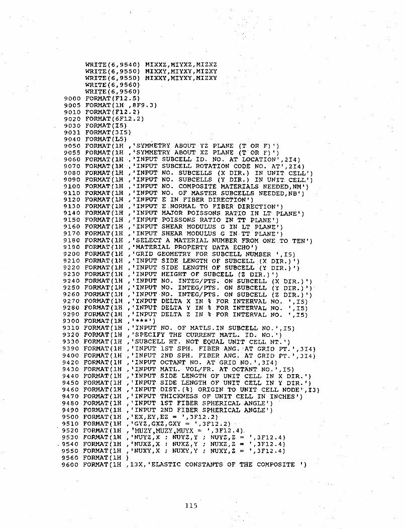
WRITE(6,9540) MIXXZ,MIYXZ,MIZXZWRITE(6,9550) MIXXY,MIYXY,MIZXYWRITE(6,9550) MIXXY,MIYXY,MIZXYWRITE(6,9560)WRITE(6,9560)
9000 FORMAT(F12.5)9005 FORMAT(IH,8F9.3)9010 FORMATIFI2.2)9020 FORMAT(6FI2.2)9030 FORMAT(I5)9031 FORMAT(315)9040 FORMAT(LS)9050 FORMAT(IH,'SYMMETRYABOUTYZ PLANE(T OR F)')9055 FORMAT(IH,'SYMMETRYABOUTXZ PLANE(T OR F) ')9060 FORMAT(IH,'INPUT SUBCELLID. NO. AT LOCATION',214)9070 FORMAT(IH,'INPUT SUBCELLROTATIONCODENO. AT',214)9080 FORMAT(IH,'INPUT NO. SUBCELLS(X DIR.) IN UNIT CELL')
9090 FORMAT(IH ,'INPUT NO. SUBCELLS (Y DIR.) IN UNIT CELL')
INPUT NO. COMPOSITE MATERIALS NEEDED,NM')
INPUT NO. OF MASTER SUBCELLS NEEDED,NB')
INPUT E IN FIBER DIRECTION')
INPUT E NORMAL TO FIBER DIRECTION')
INPUT MAJOR POISSONS RATIO IN LT PLANE')INPUT POISSONS RATIO IN TT PLANE')
INPUT SHEAR MODULUS G IN LT PLANE')
INPUT SHEAR MODULUS G IN TT PLANE')
SELECT A MATERIAL NUMBER FROM ONE TO TEN')
MATERIAL PROPERTY DATA ECHO')
GRID GEOMETRY FOR SUBCELL NUMBER ',I5)
INPUT SIDE LENGTH OF SUBCELL (X DIR.) ')
INPUT SIDE LENGTH OF SUBCELL (Y DIR.) ')
INPUT HEIGHT OF SUBCELL (Z DIR.) ')
INPUT NO. INTEG/PTS. ON SUBCELL (X DIR.)')
INPUT NO. INTEG/PTS. ON SUBCELL (Y DIR.)')
INPUT NO. INTEG/PTS. ON SUBCELL (Z DIR.)')
INPUT DELTA X IN % FOR INTERVAL NO. ',I5)
INPUT DELTA Y IN % FOR INTERVAL NO. ',I5)
INPUT DELTA Z IN % FOR INTERVAL NO. ',I5)9300 FORMAT(IH , ***')
9310 FORMAT(IH ,'INPUT NO. OF MATLS.IN SUBCELL NO.',I5)
9320 FORMAT(IH ,'SPECIFY THE CURRENT MATL. ID. NO.")
9330 FORMAT(IH , SUBCELL HT. NOT EQUAL UNIT CELL HT.')
9390 FORMAT(IH , INPUT IST SPH. FIBER ANG. AT GRID PT.',314)
9400 FORMAT(IH , INPUT 2ND SPH. FIBER ANG. AT GRID PT.',314)
9420 FORMAT(IH , INPUT OCTANT NO. AT GRID NO.',314)
9430 FORMAT(IH , _NPUT MATL. VOL/FR. AT OCTANT NO.',I5)
9440 FORMAT(IH , INPUT SIDE LENGTH OF UNIT CELL IN X DIR.')
9450 FORMAT(IH , INPUT SIDE LENGTH OF UNIT CELL IN Y DIR.')
9460 FORMAT(IH , INPUT DIST.(%) ORIGIN TO UNIT CELL NODE',I3)
9470 FORMAT(IH , INPUT THICKNESS OF UNIT CELL IN INCHES')
9480 FORMAT(IH , INPUT IST FIBER SPHERICAL ANGLE')
9490 FORMAT(IH , INPUT 2ND FIBER SPHERICAL ANGLE')
9500 FORMAT(IH , EX,EY,EZ = ',3F12.2)
9510 FORMAT(IH , GYZ,GXZ,GXY = ',3F12.2)
9520 FORMAT(IH , 'MUZY,MUZY,MUYX = ',3F12.4)
9530 FORMAT(IH , 'NUYZ,X ; NUYZ,Y ; NUYZ,Z = ',3F12.4)
.9540 FORMAT(IH ,'NUXZ,X ; NUXZ,Y ; NUXZ,Z = ',3F12.4)
9550 FORMAT(IH ,'NUXY,X ; NUXY,Y ; NUXY,Z = ',3F12.4)
9560 FORMAT(IH )
9600 FORMATIIH ,13X,'ELASTIC CONSTANTS OF THE COMPOSITE ')
9100 FORMAT(IH ,
9110 FORMAT(IH ,9120 FORMAT(IH ,
9130 FORMAT(IH ,
9140 FORMAT(IH ,
9150 FORMAT(IH ,
9160 FORMAT(IH ,
9170 FORMAT(IH ,
9180 FORMAT(IH ,
9190 FORMAT(IH ,
9200 FORMAT(IH ,
9210 FORMAT(IH ,
9220 FORMAT(IH ,
9230 FORMAT(IH ,
9240 FORMAT(IH ,
9250 FORMAT(IH ,
9260 FORMAT(IH ,
9270 FORMAT(IH ,
9280 FORMAT(IH ,
9290 FORMAT[IH ,
115

5000 ENDCC SUBROUTINETO TRANSFORMTHEC
SUBROUTINETRNS(QT,KS)DIMENSION SK(24,24)
REAL KS (24,24)
INTEGER QT
7117 FORMAT(IH , 'IN SUB TRNS,
IF(QT.GE. I00) THENDO I0 I=l,3
SN=I. 0
IF (I.EQ.3) SN=-I.0
DO i0 J=I,24
SK(I,J) =KS (I+3 ,J) *SN
SK (I+3 ,J) =KS (I ,J) *SN
SK(I+6,J) =KS (I+9,J) *SN
SK(I+9,J) =KS (I+6, J) *SN
SK(I+I2 ,J) =KS (I+15,J) *SN
SK(I+IS,J) =KS (I+12 ,J) *SNSK (I+18 ,J) =KS (I+21, J) *SN
I0 SK (I+2 i, J) =KS (I+18, J) *SNDO 20 J=l,3
SN=I. 0
IF (J.EQ. 3) SN=-I. 0
DO 20 I=i,24
KS (I,J) =SK (I, J+3) *SN
KS (I, J+3) =SK(I, J) *SN
KS (I, J+6)=SK (I,J+9) *SN
KS (I,J+9) =SK(I ,J+6) *SN
KS (I, J+12) =SK(I, J+15) *SN
KS (I,J+15) =SK (I,J+12) *SN
KS (I,J+lS) =SK (I,J+21) *SN
20 KS (I, J+2 i) =SK (I, J+lS) *SN
QT=QT-100END IF
IF (QT.GE. i0) THEN
DO I00 I=i,3
SN=-I. 0
IF(I.EQ. i) SN=I. 0DO I00 J=I,24
SK (I, J) =KS (I+9 ,J) *SN
SK (I+3, J) =KS (I+6, J) *SN
SK(I+6, J) =KS (I+3, J) *SN
SK (I+9,J) =KS (I,J) *SN
SK(I+I2 ,J)=KS (I+21,J) *SN
SK (I+15, J) =KS (I+lS, J) *SN
SK(I+I8,J) =KS (I+15,J) *SN
I00 SK(I+21,J)=KS(I+I2,J)*SNDO 200 J=l,3
SN=-I. 0
IF (J. EQ. I) SN=I. 0DO 200 I=1,24
KS (I,J] =SK(I,J+9) *SN
KS (I,J+3) =SK (I,J+6) *SN
KS (I, J+6) =SK (I, J+3) *SN
KS (I,J+9) =SK(I,J) *SN
KS (I,J+12) =SK(I,J+21) *SN
KS (I, J+15) =SK(I,J+IS) *SN
KS (I,J+18) =SK(I,J+IS) *SN
SUBCELL
QT=',I3)
STIFFNESS MATRIX
116
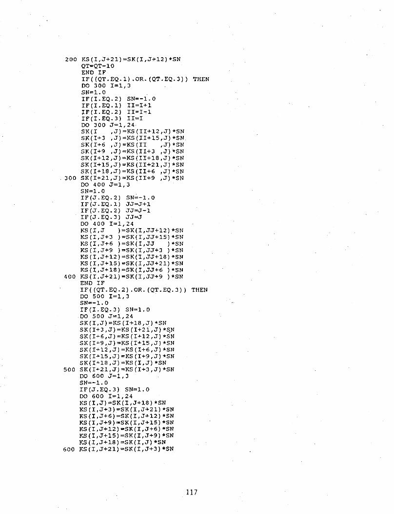
200 KS(I, J+21) =SK(I, J+12) *SNQT=QT-10ENDIFIF((QT.EQ.I) .OR.(QT.EQ.3)) THENDO300 I=i,3SN=I. 0IF(I.EQ. 2) SN=-I. 0IF(I.EQ. i) II=I+lIF(I.EQ. 2) II=I-iIF(I.EQ. 3) II=IDO300 J=i,24SK(I ,J) =KS (II+12 ,J) *SN
SK(I+3 ,J) =KS (II+15,J) *SN
SK(I_6 ,J) =KS (II ,J) *SN
SK(I÷9 ,J)=KS(II+3 ,J)*SN
SK (I+12, J) =KS (II+18, J) *SN
SK (I+15,J) =KS (II+2 i, J) *SN
SK (I+18 ,J) =KS (II+6 ,J) *SN
300 SK[I+21,J)=KS(II+9 ,J)*SN
DO 400 J=l,3SN=I. 0
IF(J.EQ. 2) SN=-I. 0
IF(J.EQ.I) JJ=J+l
IF(J.EQ.2) JJ=J-I
IF(J.EQ. 3) JJ=J
DO 400 I=i,24
KS(I,J ) =SK (I, JJ+12) *SN
KS(I,J+3 )=SK(I,JJ+IS)*SN
KS (I,J+6) =SK(I,JJ )*SN
KS(I,J+9 )=SK(I,JJ+3 )*SN
KS (I,J+12) =SK(I,JJ+I8) *SN
KS (I, J+15) =SK (I, JJ+21) *SN
KS(I,J+IS)=SK(I,JJ+6 )*SN
400 KS(I,J+21)=SK(I,JJ+9 )*SNEND I F
IF((QT.EQ.2) .OR. (QT.EQ.3)) THEN
DO 500 I=i,3SN=-I. 0
IF(I.EQ. 3) SN=I. 0
DO 500 J=i,24
SK(I ,J) =KS (I+18 ,J) *SN
SK (I+3 ,J)=KS (I+21,J) *SN
SK(I+6,J) =KS (I+12 ,J) *SN
SK (I_-9 ,J) =KS (I+15, J) *SN
SK (I÷12 ,J) =KS (I+6, J) *SN
SK(I_I5,J) =KS (I+9 ,J) *SN
SK (I_i8, J) =KS (I, J) *SN
500 SK(I_21,J)=KS(I+3,J)*SNDO 600 J=l,3
SN=-I. 0
IF(J.EQ. 3) SN=I. 0
DO 600 I=i,24
KS (I,J) =SK (I ,J+18) *SN
KS (I,J÷3) =SK (I, J+21) *SN
KS (I,J+6) =SK(I,J+I2) *SN
KS (I,J+9) =.SK (I,J+15) *SN
KS (I, J+12) =SK(I,J+6) *SN
KS (I, J+15) =SK(I, J+9) *SN
KS (I,J+lS) =SK(I, J) *SN
600 KS(I,J+21)=SK(I,J+3)*SN
117
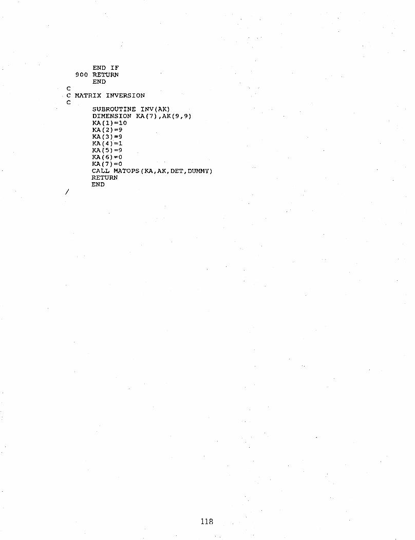
END IF
9 0 0 RETURN
END
MATRIX INVERSION
SUBROUTINE INV (AK)
DIMENSION KA(7) ,AK(9,9)
KACI) =I0KA(2) =9
KA(3)--9
KA(4):IKA(5) =9KA(6)=0KA(7) =0
CALL MATOPS (KA,AK, DET, DUMMY)RETURN
END
118
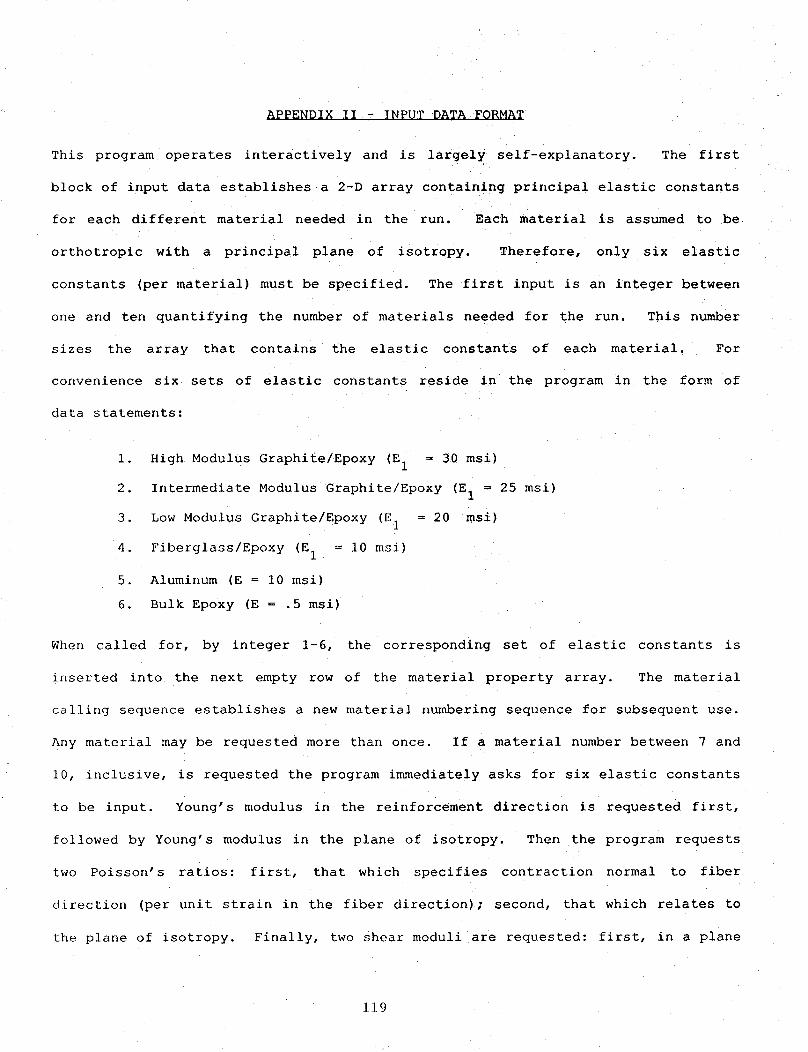
APPENDIX II - INPUT DATA FORMAT
This program operates interactively and is largely self-explanatory. The first
block of input data establishes a 2-D array containing principal elastic constants
for each different material needed in the run. Each material is assumed to be
orthotropic with a principal plane of isotropy. Therefore, only six elastic
constants (per material) must be specified. The first input is an integer between
one and ten quantifying the nun_ber of materials needed for the run. This nun_er
sizes the array that contains the elastic constants of each material. For
convenience six sets of elastic constants reside in the program in the form of
data statements:
I°
2.
3.
4.
5.
6.
When called for, by integer 1-6,
High Modulus Graphite/Epoxy (E 1 = 30 msi)
Intermediate Modulus Graphite/Epoxy (E 1 = 25 msi)
Low Modulus Graphite/Epoxy (E l = 20 msi)
Fiberglass/Epoxy (E 1 = I0 msi)
Aluminum (E = i0 msi)
Bulk Epoxy (E = .5 msi)
the corresponding set of elastic constants is
inserted into the next empty row of the material property array. The material
calling sequence establishes a new material numbering sequence for subsequent use.
Any material may be requested more than once. If a material number between 7 and
I0, inclusive, is requested the program immediately asks for six elastic constants
to be input. Young's modulus in the reinforcement direction is requested first,
followed by Young's modulus in the plane of isotropy. Then the program requests
two Poisson's ratios: first, that which specifies contraction normal to fiber
direction (per unit strain in the fiber direction); second, that which relates to
the plane of isotropy. Finally, two shear moduli are requested: first, in a plane
119
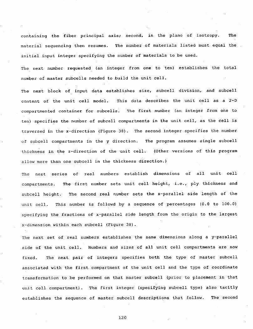
containing the fiber principal axis; second, in the plane of isotropy. The
material sequencing then resumes. The number of materials listed must equal the
initial input integer specifying the number of materials to be used.
The next number requested (an integer from one to ten) establishes the total
number of master subcells needed to build the unit cell.
The next block of input data establishes size, subcell division, and subcell
content of the unit cell model. This data describes the unit cell as a 2-D
compartmented container for subcells. The first number (an integer from one to
ten) specifies the number of subcell compartments in the unit cell, as the cell is
traversed in the x-direction (Figure 38). The second integer specifies the number
of subcell compartments in the y direction. The program assumes single subcell
thickness in the z-direction of the unit cell. (Other versions of this program
allow more than one subcell in the thickness direction.)
The next serles of real numbers establish dimensions of all unit cell
compartments. The first number sets unit cell height, i.e., ply thickness and
subcell height. The second real number sets the x-parallel side length of the
unit cell. This number is followd by a sequence of percentages (0.0 to 100.0)
specifying the fractions of x-parallel side length from the origin to the largest
x-dimension within each subcell (Figure 38).
The next set of real numbers establishes the same dimensions along a y-parallel
side of the unit cell. Numbers and sizes of all unit cell compartments are now
fixed. The next pair of integers specifies both the type of master subcell
associated with the first compartment of the unit cell and the type of coordinate
transformation to be performed on that master subcell (prior to placement in that
unit cell compartment). The first integer (specifying subcell type) also tacitly
establishes the sequence of master subcell descriptions that follow. The second
120
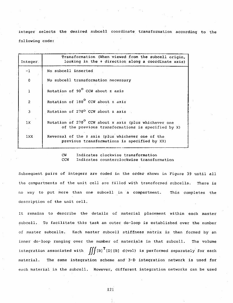
integer selects the desired subcell coordinate transformation according to the
following code:
Transformation (Whenviewed from the subcell origin,Integer looking in the + direction along a coordinate axis)
No subcell inserted-i
0
IX
IXX
No subcell transformation necessary
Rotation of 90° CCWabout z axis
Rotation of 180° CCWabout z axis
Rotation of 270° CCWabout z axis
Rotation of 270° cCW about x axis (plus whichever one
of the previous transformations is specified by X)
Reversal of the z axis (plus whichever one of the
previous transformations is specified by XX)
CW
CCW
Indicates clockwise transformation
Indicates counterclockwise transformation
Subsequent pairs of integers are coded in the order shown in Figure 39 until all
the compartments of the unit cell are filled with transformed subcells. There is
no way to put more than one subcell in a compartment. This completes the
description of the unit cell.
It remains to describe the details of material placement within each master
subcell. To facilitate this task an outer do-loop is established over the number
of master subcells. Each master subcell stiffness matrix is then formed by an
inner do-loop ranging over the number of materials in that subcell. The volume
associated with f/f[B]T[D] [B] d(vol) is performed separately for eachintegration
material. The same integration scheme and 3-D integration network is used for
each material in the subcell. However, different integration networks can be used
121

for different master subcells. What follows pertains to the integration grid
dimensions for the first master subcell.
The next real number input is the integration grids dimension in the x-direction,
followed by an integer that specifies the number of integration points on the x-
axis. This is followed by a sequence of percentages (0.0 to 100.00) specifying
the fraction of the overall grid dimension represented by the distance of each x-
axis integration point from the origin (except for the first and last values which
are assumedto be 0.0% and 100.0%).
The next two batches of input data repeat this same information for the
integration grid points along the y-axis and along the z-axis. Subsequently, an
integer is specified establishing the number of materials in the first master
subcell. This sets the upper limit on the inner do-loop that begins at this
point.
The first integer related to the inner do-loop is a material number. This selects
a set of material properties from that row of the material property matrix. The
program is now ready for detailed information on fiber orientation and amount of
material at each integration point. First, two spherical angles (_i,_2 in
degrees) specifying fiber direction (Figure II) at the first integration point,
are input, followed by the volume fraction of each octant of volume surrounding
that integration point that contains the material of interest. These volume
fractions are determined by examining photomicrographs of the actual composite and
unit cell models constructed from the same photomicrographs. To save time each
octant volume fraction is read in by means of a two number code. The first number
specifies which of the eight octants is being referenced. Octant one is the +++
octant, octant two the ++- one, octant three the +-+ one, octant four the +-- one,
octant five the -++ one, octant six the -+- one, octant seven the --+ one, and
122
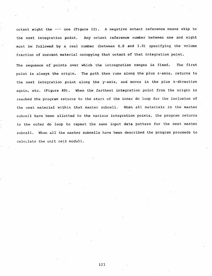
octant eight the --- one (Figure 12). A negative octant reference means skip to
the next integration point. Any octant reference number between one and eight
must be followed by a real number (between 0.0 and 1.0) specifying the volume
fraction of current material occupying that octant of that integration point.
The sequence of points over which the intregration ranges is fixed. The first
point is always the origin. The path then runs along the plus z-axis, returns to
the next integration point along the y-axis, and moves in the plus z-direction
again, etc. (Figure 40). When the farthest integration point from the origin is
reached the program returns to the start of the inner do loop for the inclusion of
the next material within that master subcell. When all materials in the master
subcell have been allotted to the various integration points, the program returns
to the outer do loop to repeat the same input data pattern for the next master
subcell. Whenall the master subcells have been described the program proceeds to
calculate the unit cell moduli.
123
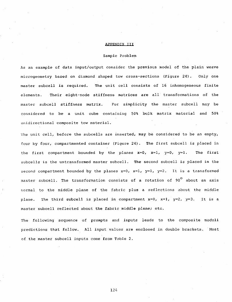
.__, - - : -
Sample Problem
As an example of data input/output consider the previous model of the plain weave
microgeometry based on diamond shaped tow cross-sections (Figure 24). Only one
master subcell is required. The unit cell consists of 16 inhomogeneous finite
elements. Their eight-node stiffness matrices are all transformations of the
master subcell stiffness matrix. For simplicity the master subcell may be
considered to be a unit cube containing 50% bulk matrix material and 50%
unidirectional composite tow material.
The unit cell, before the subcells are inserted, may be considered to be an empty,
four by four, compartmented container (Figure 24). The first subcell is placed in
the first compartment bounded by the planes x=0, x=l, y=0, y=l. The first
subcells is the untransformed master subcell. The second subcell is placed in the
second compartment bounded by the planes x=0, x=l, y=l, y=2. It is a transformed
master subcell. The transformation consists of a rotation of 90 ° about an axis
normal to the middle plane of the fabric plus a reflections about the middle
plane. The third subcell is placed in compartment x=0, x=l, y=2, y=3. It is a
master subcell reflected about the fabric middle plane; etc.
The following sequence of prompts and inputs leads to the composite moduli
predictions that follow. All input values are enclosed in double brackets. Most
of the master subcell inputs come from Table 2.
124
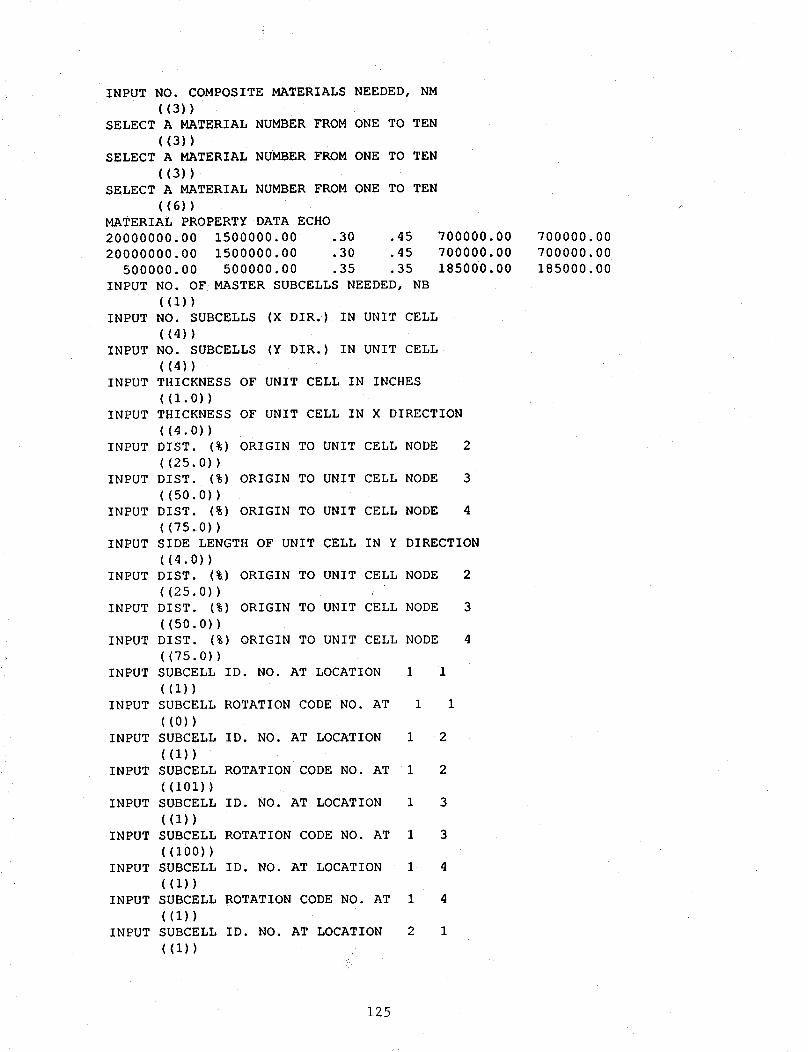
INPUTNO. COMPOSITEMATERIALSNEEDED,NM((3))
SELECTA MATERIALNUMBERFROMONETO TEN((3))
SELECT A MATERIAL NUMBER FROM ONE TO TEN
((3))
SELECT A MATERIAL NUMBER FROM ONE TO TEN
((6))
MATERIAL PROPERTY DATA ECHO
20000000.00 1500000.00 .30 .45
20000000.00 1500000.00 .30 .45
500000.00 500000.00 .35 .35
INPUT NO. OF MASTER SUBCELLS NEEDED, NB
((I))
INPUT NO. SUBCELLS (X DIR.) IN UNIT CELL
((4))INPUT NO. SUBCELLS (Y DIR.) IN UNIT CELL
((4))
INPUT THICKNESS OF UNIT CELL IN INCHES
((I.0))
INPUT THICKNESS OF UNIT CELL IN X DIRECTION
((4.0))
INPUT DIST. (%) ORIGIN TO UNIT CELL NODE 2
((25.0))
INPUT DIST. (%) ORIGIN TO UNIT CELL NODE 3
((5O. 0) )
INPUT DIST. (%) ORIGIN TO UNIT CELL NODE 4
((75.0))
INPUT SIDE LENGTH OF UNIT CELL IN Y DIRECTION
((4.0))
INPUT DIST. (%) ORIGIN TO UNIT CELL NODE 2
((25.0))
INPUT DIST. (%) ORIGIN TO UNIT CELL NODE 3
((5O.O))
INPUT DIST. (%) ORIGIN TO UNIT CELL NODE 4
((75.o) )
INPUT SUBCELL ID. NO. AT LOCATION 1 1
((I))INPUT SUBCELL ROTATION CODE NO. AT 1 1
((0))
INPUT SUBCELL ID. NO. AT LOCATION 1 2
((I))
INPUT SUBCELL ROTATION CODE NO. AT 1 2
((101))
INPUT SUBCELL ID. NO. AT LOCATION 1 3
((1))INPUT SUBCELL ROTATION CODE NO. AT 1 3
((100))INPUT SUBCELL ID. NO. AT LOCATION 1 4
((I))INPUT SUBCELL ROTATION CODE NO. AT I 4
((I))INPUT SUBCELL ID. NO. AT LOCATION 2 1
((i))
700000.00
700000.00
185000.00
700000.00
700000.00
185000.00
125
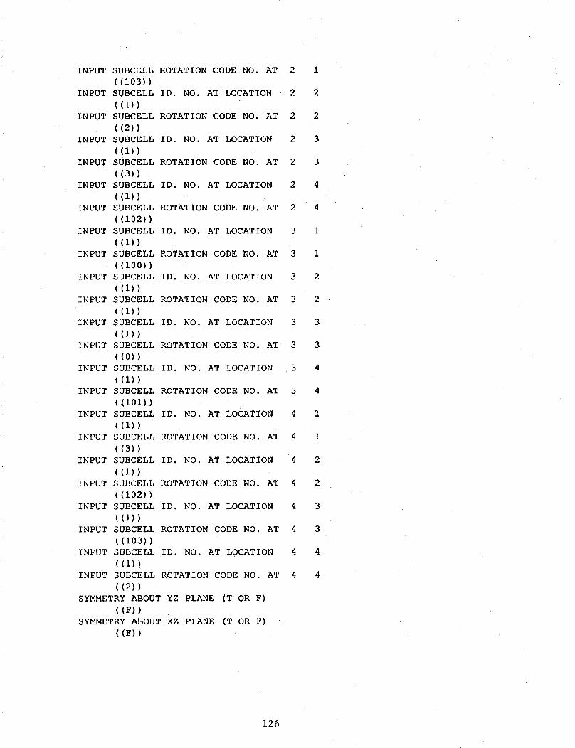
INPUTSUBCELLROTATION CODE NO. AT
((103))
INPUT SUBCELL ID. NO. AT LOCATION
((i))
INPUT SUBCELL ROTATION CODE NO. AT
((2))
INPUT SUBCELL ID. NO. AT LOCATION
((I))
INPUT SUBCELL ROTATION CODE NO. AT
((3))
INPUT SUBCELL ID. NO. AT LOCATION
((I))
INPUT SUBCELL ROTATION CODE NO. AT
((102))
INPUT SUBCELL ID. NO. AT LOCATION
((i))INPUT SUBCELL ROTATION CODE NO. AT
((IOO))
INPUT SUBCELL ID. NO. AT LOCATION
((1))INPUT SUBCELL ROTATION CODE NO. AT
((I))
INPUT SUBCELL ID NO. AT LOCATION
((i))INPUT SUBCELL ROTATION CODE NO. AT
((0))INPUT SUBCELL ID NO. AT LOCATION
((I))
INPUT SUBCELL ROTATION CODE NO. AT
((I01))
INPUT SUBCELL ID NO. AT LOCATION
((i))
INPUT SUBCELL ROTATION CODE NO. AT
((3))
INPUT SUBCELL ID NO. AT LOCATION
((1))
INPUT SUBCELL ROTATION CODE NO. AT
((102))
INPUT SUBCELL ID NO. AT LOCATION
((I))
INPUT SUBCELL ROTATION CODE NO. AT
((103))
INPUT SUBCELL ID NO. AT LOCATION
((I))INPUT SUBCELL ROTATION CODE NO. AT
((2))
SYMMETRY ABOUT YZ PLANE (T OR F)
((F))
SYMMETRY ABOUT XZ PLANE (T OR F)
((F))
2
2
2
2
2
2
2
3
3
3
3
3
3
3
3
4
4
4
4
4
4
4
4
1
2
2
3
3
4
4
1
1
2
2
3
3
4
4
1
1
2
2
3
3
4
4
126
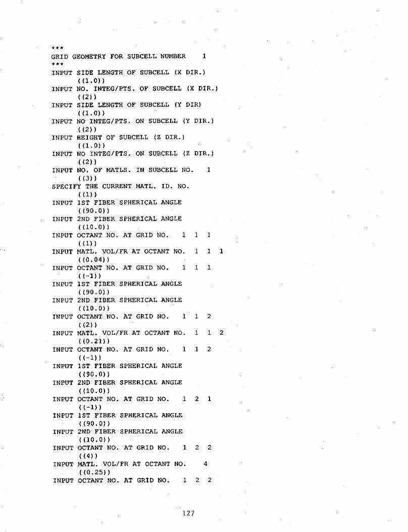
GRID GEOMETRYFORSUBCELLNUMBER 1
INPUTSIDE LENGTHOF SUBCELL(X DIR.)((i.0))
INPUTNO. INTEG/PTS.OF SUBCELL(X DIR.)((2))
INPUT SIDE LENGTH OF SUBCELL (Y DIR)
((1.0))
INPUT NO INTEG/PTS. ON SUBCELL (Y DIR.)
((2))INPUT HEIGHT OF SUBCELL (Z DIR.)
((I.0))
INPUT NO INTEG/PTS. ON SUBCELL (Z DIR.)
((2))INPUT NO. OF MATLS. IN SUBCELL NO. 1
((3))
SPECIFY THE CURRENT MATL. ID. NO.
((I))
INPUT IST FIBER SPHERICAL ANGLE
((9O.O))
INPUT 2ND FIBER SPHERICAL ANGLE
((IO.0))INPUT OCTANT NO. AT GRID NO. 1 1 I
((I))INPUT MATL. VOL/FR AT OCTANT NO. 1 1
((0.04))
INPUT OCTANT NO. AT GRID NO. 1 1 1
((-I))
INPUT IST FIBER SPHERICAL ANGLE
((9O.O))
INPUT 2ND FIBER SPHERICAL ANGLE
((i0.0))
INPUT OCTANT NO. AT GRID NO. 1 1 2
((2))INPUT MATL. VOL/FR AT OCTANT NO. 1 1
((0.21))
INPUT OCTANT NO. AT GRID NO. 1 1 2
((-I))INPUT IST FIBER SPHERICAL ANGLE
((9O.O))
INPUT 2ND FIBER SPHERICAL ANGLE
((i0.0))
INPUT OCTANT NO. AT GRID NO. 1 2 1
((-1))INPUT IST FIBER SPHERICAL ANGLE
((9O.O))
INPUT 2ND FIBER SPHERICAL ANGLE
((i0.0))
INPUT OCTANT NO. AT GRID NO. 1 2 2
((4))INPUT MATL. VOL/FR AT OCTANT NO. 4
((O.25))INPUT OCTANT NO. AT GRID NO. 1 2 2
127
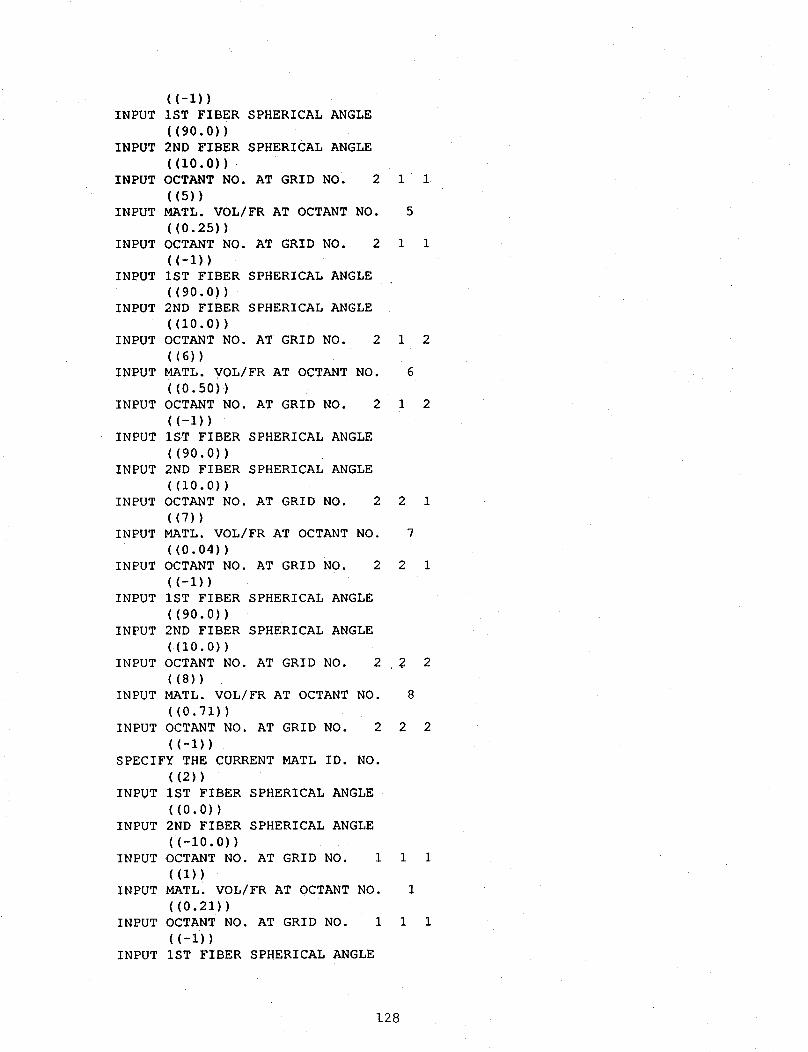
((-1))
INPUT IST FIBER SPHERICAL ANGLE
((90.0))
INPUT 2ND FIBER SPHERICAL ANGLE
((i0.0))INPUT OCTANT NO. AT GRID NO. 2 i 1
((5))INPUT MATL. VOL/FR AT OCTANT NO. 5
((0.25))
INPUT OCTANT NO. AT GRID NO. 2 1 1
((-i))
INPUT IST FIBER SPHERICAL ANGLE
((90.0))
INPUT 2ND FIBER SPHERICAL ANGLE
((I0.0))
INPUT OCTANT NO. AT GRID NO. 2 i 2
((6))
INPUT MATL. VOL/FR AT OCTANT NO. 6
((O.5O))INPUT OCTANT NO. AT GRID NO. 2 1 2
((-I))
INPUT IST FIBER SPHERICAL ANGLE
((9O.0))
INPUT 2ND FIBER SPHERICAL ANGLE
((10.0))
INPUT OCTANT NO. AT GRID NO. 2 2 1
((7))INPUT MATL. VOL/FR AT OCTANT NO. 7
((0.04))INPUT OCTANT NO. AT GRID NO. 2 2 1
((-i))
INPUT IST FIBER SPHERICAL ANGLE
((9O.0))INPUT 2ND FIBER SPHERICAL ANGLE
((I0.O))
INPUT OCTANT NO. AT GRID NO. 2 _ 2
((8))
INPUT MATL. VOL/FR AT OCTANT NO. 8
((0.71))
INPUT OCTANT NO. AT GRID NO. 2 2 2
((-I))
SPECIFY THE CURRENT MATL ID. NO.
((2))
INPUT IST FIBER SPHERICAL ANGLE
((0.0))
INPUT 2ND FIBER SPHERICAL ANGLE
((-I0.0))INPUT OCTANT NO. AT GRID NO. 1 1 1
((I))INPUT MATL. VOL/FR AT OCTANT NO. 1
((0.21))
INPUT OCTANT NO. AT GRID NO. 1 1 1
((-I))
INPUT IST FIBER SPHERICAL ANGLE
128
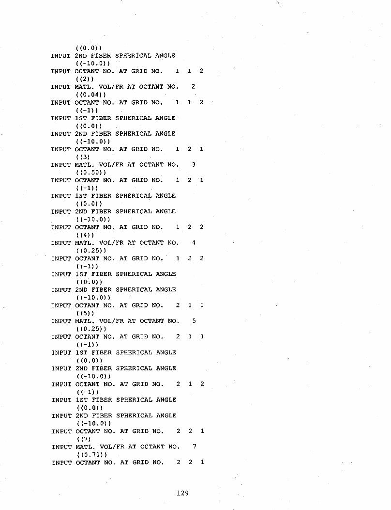
((0.0))INPUT 2ND FIBER SPHERICAL ANGLE
((-i0.0))
INPUT OCTANT NO. AT GRID NO. 1 1 2
((2))INPUT MATL. VOL/FR AT OCTANT NO. 2
((0.04))INPUT OCTANT NO. AT GRID NO. 1 1 2
((-i))INPUT IST FIBER SPHERICAL ANGLE
((0.0))
INPUT 2ND FIBER SPHERICAL ANGLE
((-i0.0))
INPUT OCTANT NO. AT GRID NO. 1 2 1
((3)INPUT MATL. VOL/FR AT OCTANT NO. 3
((O.5O))
INPUT OCTANT NO. AT GRID NO. 1 2 1
((-I))
INPUT IST FIBER SPHERICAL ANGLE
((0.0))INPUT 2ND FIBER SPHERICAL ANGLE
((-I0.0))
INPUT OCTANT NO. AT GRID NO. 1 2 2
((4))
INPUT MATL. VOL/FR AT OCTANT NO. 4
((0.25))
INPUT OCTANT NO. AT GRID NO. 1 2 2
((-I))INPUT IST FIBER SPHERICAL ANGLE
((0.0))
INPUT 2ND FIBER SPHERICAL ANGLE
((-I0.0))
INPUT OCTANT NO. AT GRID NO. 2 1 1
((5))
INPUT MATL. VOL/FR AT OCTANT NO. 5
((0.25))INPUT OCTANT NO. AT GRID NO. 2 1 1
((-I))
INPUT IST FIBER SPHERICAL ANGLE
((0.0))
INPUT 2ND FIBER SPHERICAL ANGLE
((-I0.0))INPUT OCTANT NO. AT GRID NO. 2 I 2
((-I))
INPUT IST FIBER SPHERICAL ANGLE
((0.0))
INPUT 2ND FIBER SPHERICAL ANGLE
((-I0.0))
INPUT OCTANT NO. AT GRID NO. 2 2 1
((7)INPUT MATL. VOL/FR AT OCTANT NO. 7
((0.71))
INPUT OCTANT NO. AT GRID NO. 2 2 1
129

((-1))INPUT IST FIBER SPHERICAL ANGLE
((0.0))INPUT 2ND FIBER SPHERICAL ANGLE
((-i0.0))INPUT OCTANT NO. AT GRID NO. 2 2 2
((8))
INPUT MATL. VOL/FR AT OCTANT NO. 8
((o.04) )INPUT OCTANT NO. AT GRID NO. 2 2 2
((-i))
SPECIFY THE CURRENT MATL. ID. NO.
((3))
INPUT IST FIBER SPHERICAL ANGLE
((0.0))
INPUT 2ND FIBER SPHERICAL ANGLE
((0.0))
INPUT OCTANT NO. AT GRID NO. 1 1 1
((I))
INPUT MATL. VOL/FR AT OCTANT NO. 1
((0.75))INPUT OCTANT NO. AT GRID NO. 1 1 1
((-i))INPUT IST FIBER SPHERICAL ANGLE
((o.0))INPUT 2ND FIBER SPHERICAL ANGLE
((0.0))
INPUT OCTANT NO. AT GRID NO. 1 1 2
((2))
INPUT MATL. VOL/FR AT OCTANT NO. 2
((0.75))INPUT OCTANT NO. AT GRID NO. 1 1 2
((-I))
INPUT IST FIBER SPHERICAL ANGLE
((0.0))
INPUT 2ND FIBER SPHERICAL ANGLE
((0.0))INPUT OCTANT NO. AT GRID NO. 1 2 1
((3))
INPUT MATL. VOL/FR AT OCTANT NO. 3
((O.5O))
INPUT OCTANT NO. AT GRID NO. 1 2 1
((-I))
INPUT IST FIBER SPHERICAL ANGLE
((0.0))INPUT 2ND FIBER SPHERICAL ANGLE
((0.0))
INPUT OCTANT NO. AT GRID NO. 1 2 2
((4))
INPUT MATL. VOL/FR AT OCTANT NO. 4
((0.5O))INPUT OCTANT NO. AT GRID NO. 1 2 2
((-i))
INPUT IST FIBER SPHERICAL ANGLE
130

((0.0))INPUT 2ND FIBER SPHERICAL ANGLE
((0.0))INPUT OCTANT NO. AT GRID NO. 2 1 1
((5))INPUT MATL. VOL/FR AT OCTANT NO. 5
((0.50))INPUT OCTANT NO. AT GRID NO. 2 1 1
((-I))
INPUT IST FIBER SPHERICAL ANGLE
((0.0))
INPUT 2ND FIBER SPHERICAL ANGLE
((0.0))INPUT OCTANT NO. AT GRID NO. 2 1 2
((6))INPUT MATL. VOL/FR AT OCTANT NO. 6
((0.5O))INPUT OCTANT NO. AT GRID NO. 2 1 2
((-i))
INPUT 1ST FIBER SPHERICAL ANGLE
((0.0))INPUT 2ND FIBER SPHERICAL ANGLE
((0.0))
INPUT OCTANT NO. AT GRID NO. 2 2 1
((7))
INPUT MATL. VOL/FR AT OCTANT NO. 7
((O.25))
INPUT OCTANT NO. AT GRID NO. 2 2 1
((-I))
INPUT IST FIBER SPHERICAL ANGLE
((0.0))
INPUT 2ND FIBER SPHERICAL ANGLE
((0.0))
INPUT OCTANT NO. AT GRID NO. 2 2 2
((8))
INPUT MATL. VOL/FR AT OCTANT NO. 8
((0.25))
INPUT OCTANT NO. AT GRID NO. 2 2 2
((-I))
ELASTIC CONSTANTS OF THE COMPOSITE
EX, EY, EZ = 4395007.97 4395007.97 1181426.56
GYZ,GXZ,GXY = 482009.43 482009.43 423769.42
MUYZ,MUXZ,MUXY = .1274 .1274 .1370
NUYZ,X ; NUYZ,Y ; NUYZ, Z = .0000 .0000 .0000
NUXZ,X ; NUXZ,Y ; NUXZ, Z = .0000 .0000 .0000
NUXY,X ; NUXY, Y ; NUXY,Z = .0000 .0000 .0000
131
Form Approved
OMB No. 0704-0188REPORT DOCUMENTATION PAGE
P'_QIIC rel_Orl_lR_ Durden fol" tRi$ collection of information ;s estlmat_cl to averaqe ; hour oer respor_$e, including the time for rewewmg insti'uc_ions, _earcnmq exrstlng elate sources.
_atherlng and malntammg the data nee_ecl, and ¢ompietlncj ancl reviewing the collection ot _nformatlon. Sena comments regarding this bucaen esttmate ot any other aspect of _.hl$collection of information. _nctuding suggest!ons for r_=_iuclng this Duraen. to W_tshJngton Headcluarters Services, Dire_orate for Information OPerations and ReDort$, 1215 Jefferson
Oavls Highway, Suite 1204, Arlington, VA 222024302, anti tO the Office of Management and Budcjet, Paperwork Reduction Prc ject (0704-0188), Wasr',ington, OC 20503.
1. AGENCY USE ONLY (Leave blanK) 2. REPORT DATE 3. REPORT TYPE AND DATES COVERED
February 199:_ C,_ntractorReoort14. TITLE AND SUBTITLE
FiniteElementAnalysisof the Stiffnessof FabricReinforcedComposites
6. AUTHOR(S)
R. L Foye
7. PERFORMING ORGANIZATION NAME(S) AND ADDRESS(ES)
Lockheed Engineering and Sciences Company144 Research Drive
Hampton, VA 23666
9. SPONSORING/MONITORING AGENCY NAME(S) AND ADDRESS(ES)
National Aeronautics and Space Administration
Langley Research Center
Hampton, VA 23665-5225
5. FUNDING NUMBERS
C NASI-19000
505-63-50-04
8. PERFORMING ORGANIZATIONREP_JRT NUMBER
10. SPONSORING/MONITORINGAGENCY REPORT NUMBER
NASA CR-189597
11. SUPPLEMENTARY NOTES
Langley Technical Monitor: H. Benson Dexter/C. C. Poe
12a. DISTRIBUTION / AVAILABILITY STATEMENT
Unclassified-Unlimited
Subject Category 24
12b. DISTRIBUTION CODE
13. ABSTRACT (Maximum 200 words)
The objective of this work is the prediction of all 3-D elastic moduli of textile fabric reinforced composites. The analysis is
general enough for use with complex reinforcing geometries and capable of subseqUent improvements. It places norestrictions on fabric microgeometry except that the unit cell be determinate and rectangular. The unit cell is divided into
rectangular subcelis in which the reinforcing geometries are easier to define and analyze. The analysis, based on
inhomogeneous finite elements, is applied to a variety of weave, braid, and knit reinforced composites. Some of these
predictions are correlated to test data.
14. SUBJECT TERMS
Fabrics;Elasticproperties;Finiteelement analysis
17. SECURITY CLASSIFICATION 18. SECURITY CLASSIFICATION 19. SECURITY CLASSIFICATIONOF REPORT OF THIS PAGE _ OF ABSTRACT
I I m_,l _Nc;,,_I
NSN 7540-01-280-5500I I _¢._.= _ _ _,,w=4 !
15. NUMBER OF PAGES
137 -16. PRICE CODE
#07 ....-
20. LIMITATION ()F ABSTRACT
Standard Form 298 (Rev. 2-89)PrescrliOed t_y _NSI Std. Z39-18
='78-_02