nasa contractor report 4687
TRANSCRIPT

NASA Contractor Report 4687
N96-148Bt
Uncll as
HfJfS Q06479f

NASA Contractor Report 4687
An Open Loop Guidance Architecture for Navigationally Robust On-Orbit Docking Hung-Sheng Chern The George Washington University Joint Institute for Advancement of Flight Sciences Langley Research Center 0 Harnpton, Virginia
National Aeronautics and Space Administration Langley Research Center * Hampton, Virginia 23681 -0001
Prepared for Langley Research Center under Cooperative Agreement NCC1-104

Printed copies available from the following:
NASA Center for Aerospace Information 800 Elkridge Landing Road Linthicum Heights, MD 21090-2934 (301) 621-0390 (703) 487-4650
National Technical Information Service (NTIS) 5285 Port Royal Road Springfield, VA 22161-2171

Abstract
The development of an open-loop guidance architecture is outlined for autonomous
rendezvous and docking (AR&D) missions to determine whether the Global Position-
ing System (GPS) can be used in place of optical sensors for relative initial position
determination of the chase vehicle. Feasible command trajectories for one, two, and
three impulse AR&D maneuvers are determined using constrained trajectory opti-
mization. Early AR&D command trajectory results suggest that docking accuracies
are most sensitive to vertical position errors at the initial condition of the chase ve-
hicle. Thus, a feasible command trajectory is based on maximizing the size of the
locus of initial vertical positions for which a fixed sequence of impulses will trans-
late the chase vehicle into the target while satisfying docking accuracy requirements.
Documented accuracies are used to determine whether relative GPS can achieve the
vertical position error requirements of the impulsive command trajectories. Prelim-
inary development of a thruster management system for the Cargo Transfer Vehicle
(CTV) based on optimal throttle settings is presented to complete the guidance archi-
tecture. Results show that a guidance architecture based on a two impulse maneuver
generated the best performance in terms of initial position error and total velocity
change for the chase vehicle.
iii


Contents
Abstract iii
List of Figures vii
List of Tables X
Nomenclature xi
1 Introduction 1
1.1 Types of Rendezvous Maneuvers . . . . . . . . . . . . . . . . . . . . . 1
1.2 Current Sensor Technology . . . . . . . . . . . . . . . . . . . . . . . . 2
1.3 Global Positioning System Overview . . . . . . . . . . . . . . . . . . 3
1.4 Scope of Investigation . . . . . . . . . . . . . . . . . . . . . . . . . . 4
1.4.1 Feasible Command Trajectories . . . . . . . . . . . . . . . . . 5
1.4.2 Thruster Management System . . . . . . . . . . . . . . . . . . 6
2 Mission Description 7
2.1 Basic Assumptions . . . . . . . . . . . . . . . . . . . . . . . . . . . . 7
2.2 Vehicle Model . . . . . . . . . . . . . . . . . . . . . . . . . . . . . . . 7
2.3 Mission Constraints . . . . . . . . . . . . . . . . . . . . . . . . . . . . 10
2.3.1 Basic Target Constraints . . . . . . . . . . . . . . . . . . . . . 10
2.3.2 Additional Constraints . . . . . . . . . . . . . . . . . . . . . . 11
3 Single Impulse AR&D Maneuver 14
3.1 Constrained Trajectories . . . . . . . . . . . . . . . . . . . . . . . . . 15

3.1.1 Two Trajectory Formulation . . . . . . . . . . . . . . . . . . . 15
3.1.3 Quadratic-Fit Formulation . . . . . . . . . . . . . . . . . . . . 18
3.2 Single Impulse AR&D Results . . . . . . . . . . . . . . . . . . . . . . 22
3.2.1 Optimized Results for a Single Initial Position . . . . . . . . . 22
3.2.2 Family of Optimized Results . . . . . . . . . . . . . . . . . . . 26
3.1.2 Three Trajectory Formulation . . . . . . . . . . . . . . . . . . 17
4 Two Impulse AR&D Maneuver 29
4.1 Optimization Formulation . . . . . . . . . . . . . . . . . . . . . . . . 30
4.2 Two Impulse AR&D Results . . . . . . . . . . . . . . . . . . . . . . . 31
4.2.1 Optimization Results . . . . . . . . . . . . . . . . . . . . . . . 31
4.2.2 Simulation Results . . . . . . . . . . . . . . . . . . . . . . . . 34
5 Three Impulse AR&D Maneuver 42
5.1 Optimization Formulation . . . . . . . . . . . . . . . . . . . . . . . . 42
5.2 Three Impulse AR&D Results . . . . . . . . . . . . . . . . . . . . . . 43
6 Thruster Management System 48
6.1 Cargo Transfer Vehicle (CTV) . . . . . . . . . . . . . . . . . . . . . . 48
6.2 Thruster Firing Concept . . . . . . . . . . . . . . . . . . . . . . . . . 50
6.2.1 Formulations for Optimal CTV Thruster Firings . . . . . . . . 51
6.2.3 Representative Throttle Setting Results . . . . . . . . . . . . . 52
6.2.2 Solving the Thruster Firing Optimization Problem . . . . . . 52
7 Summary and Recommendations 55
Bibliography 58
A Early AR&D Formulations 60
A. l Early AR&D Problem Statement . . . . . . . . . . . . . . . . . . . . 60
A.2 Early AR&D Results . . . . . . . . . . . . . . . . . . . . . . . . . . . 61
I3 Quadratic Behavior at Target Vehicle
vi
64

List of Figures
1.1
2.1
2.2
3.1
3.2
3.3
3.4
3.5
3.6
3.7
3.8
3.9
Open-loop guidance architecture . . . . . . . . . . . . . . . . . . . . . 4
Coordinate system geometry . . . . . . . . . . . . . . . . . . . . . . . Maneuver constraints geometry . . . . . . . . . . . . . . . . . . . . .
9
12
Maximum vertical tolerance target constraint for the chase vehicle . . Vertical tolerance constraint comparison between two trajectory and
three trajectory formulations . . . . . . . . . . . . . . . . . . . . . . . Vertical tolerance constraint comparison between two trajectory, three
trajectory, and three trajectory with quadratic constraint formulations
Horizontal relative position for chase vehicle starting at xo = 600 ft . Vertical relative position for chase vehicle starting at xo = 600 ft . . . Trajectory simulation for the chase vehicle starting at xo = 600 ft . . Early trajectory for the chase vehicle starting at xo = 600 f t . . . . . Final approach trajectory for chase vehicle starting at xo = 600 ft . . Performance robustness with respect to initial relative horizontal chase
vehicle position . . . . . . . . . . . . . . . . . . . . . . . . . . . . . .
16
18
21
23
24
24
25
25
27
3.10 Initial impulse components with respect to initial relative horizontal
chase vehicle position . . . . . . . . . . . . . . . . . . . . . . . . . . . 3.11 Initial impulse speed with respect to initial relative horizontal chase
vehicle position . . . . . . . . . . . . . . . . . . . . . . . . . . . . . . 3.12 Terminal chase vehicle speed with respect to initial relative horizontal
chase vehicle position . . . . . . . . . . . . . . . . . . . . . . . . . . .
27
28
28
vii

4.1
4.2
4.3
4.4
4.5
4.6
4.7
4.8
4.9
Performance robustness for two impulse maneuver at xo = 600 f t . . . Variation of initial impulse components at xo = 600 ft . . . . . . . . . Variation of second impulse components at xo = 600 ft . . . . . . . . Impulse speeds with respect to second impulse time at xo = 600 f t . . Total speed change with respect to second impulse time at 20 = 600 ft
Gate and target times for upper trajectories at xo = 600 ft . . . . . . Two impulse simulation for chase vehicle starting at xo = 600 ft with
a second impulse time of 3000 seconds . . . . . . . . . . . . . . . . . Two impulse final approach trajectories for the chase vehicle starting
at 20 = 600 ft with a second impulse time of 3000 seconds . . . . . . Horizontal relative position for chase vehicle starting at 50 = 600 ft
with a second impulse time of 3000 seconds . . . . . . . . . . . . . . .
31
32
32
33
33
35
36
36
37
4.10 Vertical relative position for chase vehicle starting at xo = 600 ft with
. . . . . . . . . . . . . . . . . 4.11 Two impulse simulation for chase vehicle starting at 20 = 600 ft with
. . . . . . . . . . . . . . . . . 4.12 Horizontal relative position for chase vehicle starting at xo = 600 ft
with a second impulse time of 1000 seconds . . . . . . . . . . . . . . . 4.13 Vertical relative position for chase vehicle starting at 20 = 600 ft with
. . . . . . . . . . . . . . . . . 4.14 Two impulse simulation for chase vehicle starting at xo = 600 ft with
a second impulse time of 5000 seconds . . . . . . . . . . . . . . . . . 4.15 Horizontal relative position for chase vehicle starting at xo = 600 ft
with a second impulse time of 5000 seconds . . . . . . . . . . . . . . . 4.16 Vertical relative position for chase vehicle starting at xo = 600 ft with
.
a second impulse time of 3000 seconds 37
a second impulse time of 1000 seconds 38
39
a second impulse time of 1000 seconds 39
40
40
a second impulse time of 5000 seconds . . . . . . . . . . . . . . . 41
5.1 Performance robustness with respect to second and third impulse times
at xo = 600 ft . . . . . . . . . . . . . . . . . . . . . . . . . . . . . . . Performance robustness with respect to third impulse times. . . . . .
45
46 5.2
viii

6.1
6.2
Optimal throttle settings for positive axial direction unit impulses . . Optimal throttle settings for negative axial direction unit impulses . .
53
54
A.l Early AR&D footprint results of admissible position errors at the chase
vehicle initial condition . . . . . . . . . . . . . . . . . . . . . . . . . . 62
A.2 Early AR&D trajectory simulation starting from the extreme ends of
admissible initial vertical chase positions . . . . . . . . . . . . . . . . 63
B.1 Perturbation results of 2 using optimized single-impulse results at
~o=600 ft . . . . . . . . . . . . . . . . . . . . . . . . . . . . . . . . . 67
ix

List of Tables
2.1 Target accuracy requirements . . . . . . . . . . . . . . . . . . . . . . 10
2.2 Gate constraint position . . . . . . . . . . . . . . . . . . . . . . . . . 12
5.1 Percent increase comparisons between the two impulse command tra-
jectory and the three impulse command trajectory . . . . . . . . . . . 47
6.1 CTV thruster location and force vector directions . . . . . . . . . . . 49
6.2 CTV and payloads mass properties . . . . . . . . . . . . . . . . . . . 50
X

Nomenclature
Symbols
a
C
CTV thruster throttle setting
function weighting values for Do function weighting values for D1 function weighting values for D2
CTV optimal control constraint relations vector
constraint relations
second-order polynomial coefficients
normalized CTV thruster forces vectors
constraint relation between final chase vehicle position and
maximum target tolerance, in
target vehicle orbital altitude, ft
cost function
Lagrangian
second-order Lagrange interpolating polynomials
nth-order Lagrange interpolating polynomials
interpolated polynomial
quadratic polynomial to model evf
in-plane radial distance component for polar coordinate system
thruster location with respect to CTV body axis, ft
CTV thruster model
xi

X
Y
Y e
At
AV
A%
t
X g a t e
Y g a t e
Y t a r g
VtO,Tg
in-plane horizontal distance component for Cartesian coordinate
system
in-plane vertical distance component for Cartesian coordinate
system
point of occurance for maximum value of q(y)
total transfer time, sec
total velocity change of the chase vehicle, in/s
total velocity of the chase vehicle associated with the
initial impulse, in/s
total velocity of the chase vehicle associated with the
second impulse, in/s
total velocity of the chase vehicle associated with the
third impulse, in/s
variational operat or
Lagrange multiplier vector
orbital angular velocity, rad/s
in-plane state transition matrix
in-plane angular sweep in polar coordinate system
locus of initial chase vehicle vertical positions, ft
admissible initial vertical error, in
set of free parameters for one, two, and three impulse
maneuvers, respectively
time, sec
horizontal position of gate constraint, ft
vertical position of gate constraint, ft
vertical position tolerance at target, in
maximum docking speed, in/s
xii
Subscripts
0
f gate
i .. 22
targ
time1
time2
AR&D
CTV
DOF
EP
GPS
H.O.T.
IMU
LaRC
LEO
MSFC
NASA
NAVSTAR
TOPEX
at initial position
at final time
at gate geometry
at second impulse
at third impulse
at target vehicle
time constraint relation for two impulse command trajectories
time constraint relation for three impulse command trajectories
Superscripts
derivative with respect to time
vector
Acronyms
autonomous rendezvous and docking
cargo transfer vehicle
degree-of- freedom
explorer platform
global positioning system
higher-order terms
inertial measurement unit
Langley Research Center
low-Earth orbit
Marshall Space Flight Center
National Aeronautics and Space Administration
navigation system using timing and ranging
ocean topography experiment
xiii


Chapter 1
Introduction
Present rendezvous and docking procedures for the U.S. space program have relied
heavily upon crew and ground involvement. The most taxing of all the phases in a
rendezvous and docking mission is arguably the terminal phase of the rendezvous.
Under present conditions, the pilot operations take precedence over nearly all the on-
board guidance and navigation. The terminal approach is performed manually using
visual cues and proximity data from extremely accurate sensors. However, rendezvous
systems of this type are highly susceptible to pilot error and, considering the cost and
complexity of the subsystems required, are expensive to perform on a regular basis.
The future of the space program include plans for rendezvous and docking missions
such as satellite servicing and unmanned cargo resupply of Space Station Freedom.
Thus, the development of a reliable autonomous rendezvous and docking maneuver
is an integral step for progress in the space program. The foundation for a reli-
able AR&D maneuver is a navigational system which can accurately provide relative
position and velocity throughout the entire docking procedure.
1.1 Types of Rendezvous Maneuvers
There exist two different types of terminal phase rendezvous maneuvers - docking and
berthing maneuvers. In general, both types of procedures involve the maneuvering of
a chase vehicle to meet a target vehicle in orbit so that the two vehicles can couple,

presumably for purposes of mass transfer. Specifically, docking refer to maneuvers in
which the chase vehicle flies directly into the target with a nonzero final velocity [l].
Berthing maneuvers refer to the use of an intermediate device, such as a manipulator
arm, to grapple the chase vehicle as it is brought to a relative standstill near the
target [l]. Thus, berthing maneuvers do not require a closing velocity between the
two vehicles. While docking maneuvers provide the simplest means of coupling two
vehicles in orbit, they do introduce some risk in the areas of collision, guidance,
navigation, and control.
1. .2 Current Sensor Technology
Some of the most common sensors used to determine relative position are visual sen-
sors and laser navigation sensors. These sensors are used since they can obtain the
highly stringent accuracy requirements associated with terminal phase rendezvous
and docking maneuvers. Visual sensors, such as video-only cameras and sophisti-
cated automatic pattern recognition cameras [2], are susceptible to adverse lighting
conditions and require high computer throughput [3]. Laser navigation systems re-
quire the placement of reflectors on the target. Thus, a highly accurate knowledge
of the reflector location relative to the target vehicle coordinate system is required.
This essentially means that a complete knowledge of the target vehicle attitude is
necessary for an accurate laser measurement.
Both systems essentially require a direct line-of-sight between the chase and target
vehicle. This partially accounts for the so-called R-bar and V-bar terminal approaches
associated with current rendezvous and docking procedures in which the chase vehicle
flies directly towards the target along the radial or tangential directions, respectively.
While these two conventional navigation systems have provided adequate results
for present rendezvous and docking missions, future autonomous rendezvous and
docking (AR&D) missions, particular for unmanned vehicles, require a system that
provides sufficiently accurate results while, at the same time, is not restricted by some
of the limitations of visual sensors and laser navigation.
2

1.3 Global Positioning System Overview
The Global Positioning System (GPS) is a constellation of navigation satellites and
is a means of providing the US. military with accurate latitude, longitude, altitude,
travel velocity, and time under any environmental conditions. This system was ini-
tially proposed in the 1970’s with the first Navigation System using Timing And
Ranging (NAVSTAR) GPS satellite launched in 1978 [4]. The present constellation
consists of 24 satellite positions at an altitude of 10,924 nmi, with four satellites at
each of the six 55 deg inclined equally spaced orbital planes [5] .
GPS technology has developed to the point where it is now a means of providing
an ideal on-board precision navigation and pointing capability for Low Earth Orbit
(LEO) missions [6]. In fact, several flight experiments have been proposed which
incorporate the use of GPS position and attitude determination for AR&D missions.
One such proposed flight demonstration suggests an AR&D mission between a small,
low-cost, NASA satellite powered by batteries and a cold gas thruster and the Ex-
plorer Platform (EP) Spacecraft. Under this proposed scenario, the sensor system
is comprised of a GPS receiver, a laser illuminator, and a video camera. The GPS
receiver is used for both absolute and relative positioning for coarse guidance of up
to 330 ft while the laser illuminator and the video camera are used for fine guidance
c71. However, relative GPS position determination has improved to the point where
inch accuracies are possible. Recent precision orbit determination experiments with
the Ocean Topography Experiment (TOPEX)/Poseidon satellite have obtained radial
ephemeris RMS difference accuracies to within 1.18 - 1.57 inches [SI. Ground sur-
veying experiments using relative GPS have also obtained inch accuracies in relative
position determination [9].
However, these accuracies are based on GPS data transmitted through the atmo-
sphere. Thus, these accuracies can be affected by tropospheric delays, ionospheric
delays, and multipath errors due to ground structures. In this study, it is conceivable
that relative GPS accuracies between orbiting vehicles are much better than those
3

previously documented. Recent evaluations of relative GPS position determination
for AR&D missions has shown that it is theoretically possible to obtain relative posi-
tion accuracies to within 0.394 inches [lo]. Thus, it may be possible to replace optical
sensors with relative GPS as a cheaper means of navigation.
1.4 Scope of Investigation
The scope of this investigation is to develop an open-loop guidance architecture for
the terminal phase of an AR&D mission to determine whether relative GPS can be
used in place of optical sensors. Figure (1.1) illustrates a schematic of the open-loop
system.
threshold _ _ - __ _ _
I
> non-realtim Avfc,Av2c thruster re/ative GPS
Avfbv2 5. vehicle
sequencer I management i initial
Figure 1.1: Open-loop guidance architecture
4

The first step in the open-loop system is the use of non-real time relative GPS to
determine the initial position of the chase and target vehicles. Once the threshold
accuracy for the relative position between the vehicles is achie , the chase vehicle
is given a fixed sequence of pre-determined AV commands. The final step in the
open-loop process is the execution of the commands from the AV sequencer by the
thruster management system. In addition to the firing laws, the thruster management
system includes an inertial measurement unit (IMU). Thruster management laws can
be affected by errors that are cause by finite burn-time effects and thruster errors.
For short periods, the IMU would be used to correct these errors. The development
of the guidance architecture is done in two steps. First, feasible command trajecto-
ries are determined for one, two, and three impulse maneuvers. Second, a thruster
management system is developed to execute these command trajectories.
1.4.1 Feasible Command Trajectories
In this study, feasible command trajectories govern the fixed sequences of impulses.
These trajectories are determined for one, two, and three impulse AR&D maneuvers.
Previous impulsive guidance research suggests that accuracies at docking are most
sensitive to vertical position errors at the initial condition of the chase vehicle and
is rather insensitive to horizontal position errors (see Appendix A). Thus, command
trajectories are determined by using optimization methods to maximize the range
of admissible initial vertical position errors of the chase vehicle. The maximized
admissible vertical position errors for each of the command trajectories are compared
to navigational accuracies attainable through relative GPS to determine whether it
is a viable maneuver. Chapter 2 outlines the vehicle model, mission parameters, and
mission constraints. Chapters 3, 4, and 5 detail the optimization formulation and
command trajectory results for the various impulse maneuvers.
5

1.4.2 Thruster Management System
The approach in developing the thruster management system is to determine opti-
mal throttle settings for the chase vehicle thrusters to realize the impulse commands
for the feasible command trajectories. A modulator is then required to determine
minimum firing times based on these optimal throttle settings. This study presents
the preliminary design of the thruster management system by developing the formu-
lations to determine these optimal throttle settings. Chapter 6 outlines the specific
chase vehicle thruster model and the basic optimization formulations.
6

Chapter 2
Mission Description
This chapter presents the basic assumptions for the mission, the vehicle model, the
mission parameters, and the mission constraints for the terminal phase AR&D ma-
neuver.
2 , l Basic Assumptions
There are several basic assumptions which govern the type of AR&D maneuver de-
termined by the command trajectories. First, it is assumed that the chase vehicle
is on-orbit with the target and trails the target by some given distance, say 600 ft.
While in its initial position, the chase vehicle is assumed to have no relative motion
with respect to the target. Also, the docking mechanism is assumed to be located on
the far side of the target vehicle. This requires an AR&D maneuver where the chase
vehicle must fly to the front of the target vehicle to complete the docking mission.
Finally, to obtain the highest degree of relative position accuracy using relative GPS,
issues such as integer ambiguity and cycle slip are assumed to be resolved.
2-2 Vehicle Model
Several assumptions are made concerning the vehicle model. Since this study involves
the terminal phase of an AR&D maneuver, equations are determined which govern
7

the motion of the chase vehicle relative to the target vehicle for small perturbations
about a reference orbit. In this case, the reference orbit is assumed to be the circular
orbit of the target vehicle. This naturally assumes that the radial component of
the target velocity does not change with respect to time and with respect to the
orbital position. Conversely, if the reference orbit had a slight eccentricity, such
an assumption concerning the radial velocity component of the target vehicle would
not be true. Furthermore, the orbital angular velocity of the target vehicle, w, is
also assumed to be constant. Thus, the transfer angle between the chase and target
vehicle is simply the product of the angular velocity and the transfer time At.
The dynarnical model and coordinate system for the rendezvous and docking mis-
sion are constituted by the Clohessy-Wiltshire equations [ll]. This is a Cartesian
coordinate system centered on a target assumed to be in a circular orbit and involves
linear time-invariant dynamics. The Clohessy-Wiltshire equations are also known as
Hill’s equations and have been used to analyze the relative motion of two satellites
in orbit in close proximity to each other. The model presented in this report rep-
resent the motion in the vertical plane. The geometry is shown in Fig. (2.1). The
target-centered Cartesian coordinate system is orientated such that the y-axis is al-
ways pointing radially outward from the center of the Earth and the x-axis is pointing
in the opposite direction of the target vehicle velocity vector. In this representation,
the x and y-axes are in the orbit plane.
For the target-centered coordinate system, the in-plane linearized equations of
relative motion for the chase vehicle are Ell]
8
(2.1) .

Y A Target
Safellite Chaser 5afeM?e
- 1 6(wAt - sin w A t ) sin w A t - 3 A t $( 1 - cos w A t )
0 4 - 3 cos w A t ?( 1 - cos w A t ) sin w A t
0 6w( 1 - CoswAt) 4 COS w A t - 3 2 sin w A t
0 3w sin w A t -2 sin w A t cos w A t
(ain( At) =
-
/ ~ , E ~ M e r e n c e O r b i f
Relative Coordinate System
(2-3)
Figure 2.1: Coordinate system geometry
The solution to Eqn. (2.1) results in an in-plane chase vehicle motion governed
by [111
where
Yo = (ai,( At)
r
9

2.3 Mission Constraints
This section presents the target accuracy requirements of the AR&D mission and the
motivation behind and the requirements of the gate constraints.
2.3.1 Basic Target Constraints
The orbital altitude, h, of the target vehicle is approximately 255 mi. Table (2.1)
lists the allowable position and velocity tolerances at the target for the chase vehicle.
For this particular AR&D problem, the chase vehicle must be within a vertical (y-
axis) accuracy of f0.591 in and a maximum speed tolerance of 0.591 in/s (priv.
communication - Mr. Fred Roe, MSFC - April 30, 1993). These constraints assume
that the chase vehicle motion is restricted to the orbital plane.
Table 2.1 : Target accuracy requirements
With the docking accuracies set, the target constraints for the constrained opti-
mization problem which must be satisfied by the chase vehicle are represented as
Ctarg = (2.4) y ( t t a r g ) I Ytarg
y(ttu7.g) L -Ytarg
k 2 ( t t a r g ) + G2( t targ ) I Vt"arg where ytarg > 0. The first of Eqn. (2.4) requires that the chase vehicle physically
docks with the target at the transfer time of tturg. The remainder of Eqn. (2.4)
are the vertical position tolerance and the maximum speed tolerance summarized in
Table (2.1).
10

2.3.2 Additional Constraints
Previously unpublished work has been done for this type of impulsive AR&D com-
mand trajectory. Appendix A outlines the basic formulation and presents some basic
results for this earIy AR&D research. In summary, the early AR&D results suggests
two points. First, accuracy at docking seems most sensitive to the initial vertical PO-
sition errors of the chase vehicle. Second, early simulation results show that, with just
target constraints, optimized trajectories for the chase vehicle tend to approach the
target tangentially. While handling vertical position sensitivity is presented later in
this work, the simulation results shown in Fig. (A.2) justify the need for additional
chase vehicle constraints to generate a more direct and predictable final approach
towards the target vehicle.
For this particular problem, it is assumed that the target docking port is facing the
same direction as the target vehicle velocity vector. Thus, the command trajectory
for the chase vehicle must approach the target from the negative x-axis. While any
docking approach could have been chosen, this particular type of approach takes
advantage of the target vehicle velocity. Recall that the target motion is in the
negative x-axis direction. A final approach trajectory from that direction requires
less total velocity change by the chase vehicle. To generate such a trajectory, a
gate constraint placed at an arbitrary position ahead of the target is added to the
optimization problem. Figure (2.2) displays the desired final approach trajectory for
the chase vehicle. The exact position of the gate geometry relative to the target is
listed in Table (2.2). While these particular parameters are arbitrarily chosen, an
appropriate gate position for actual flight experiments would be highly dependent
upon the configuration of the chase and target vehicles. The gate position must be
chosen such that the docking procedure does not result in any collisions between
possible extended appendages present in the vehicle configurations. Note that the
illustration in Fig. (2.2) is not drawn to scale.
11

k----lOft Gate Geometry
ygate Target Geometry +5 ft
Figure 2.2: Maneuver constraints geometry
Table 2.2: Gate constraint position n I 11
Category Accuracy
12

Based on this trajectory approach requirement, the gate constraints for the chase
vehicle are represented as
i ( t g a t e ) L 0
5 ( t g a t e ) = zgate
Y ( t g a t e ) I Ygate
Y ( t g a t e ) 2 -ygate
Cgate =
where ygate > 0. The first portion of Eqn. (2.5) is the mathematical representation
that the chase vehicle must eventually approach the target from the negative x-axis
direction at the transfer time of tgate. The remaining portions of Eqn. (2.5) are just
the geometric constraints listed in Table (2.2).
As a final assurance that the approach trajectory is from the negative x-axis
direction, an additional constraint must be added to Eqn. (2.4). Equation (2.6)
controls the horizontal component of the chase vehicle velocity at the target insuring
that the final chase vehicle motion is in the positive x-axis direction.
To completely quantify this final approach trajectory, Eqn. (2.6) must be added
to the target constraints. Thus, the complete target constraints for the constrained
optimization problem are expressed as
13

Chapter 3
Single Impulse AR&D Maneuver
This chapter develops a single impulse command trajectory. The single impulse com-
mand trajectory is determined by maximizing the locus of initial vertical positions
for which a single impulse translates the chase vehicle into the target while satisfying
all gate and target constraint conditions outlined in Chapter 2. This locus of vertical
positions is expressed as
Yo = {Y = Yo + SY, ISY I I AYOI (3.1)
The scalar cost function for the AR&D trajectory optimization is, accordingly,
where Ayo > 0. For each command trajectory, the free parameters of the problem
are zo, YO, AYO, 50, Yo, (ttarg)y7 and ( t g a t e ) y - The parameters ( t t a r g ) y and ( t g a t e ) y
correspond to target and gate times for different trajectories emanating from (zo, y)
where y e yo. In the results generated for the single impulse command trajectories,
the parameter zo is selected by the user. To simplify the notation, the set of free
parameters for each trajectory in the single impulse maneuver is expressed as
14

While results are presented for the single impulse AR,&D command trajectories,
the initial portion of this chapter illustrate the individual steps taken in the research
to mathematically determine this locus of admissible initial vertical positions for the
chase vehicle.
3.1 Constrained Trajectories
While maximizing Ayo provides a means of determining this locus of initial vertical
positions, no mention has yet been made on how to represent Ayo. In this section, the
steps taken in the research are presented individually to show how a set of constrained
trajectories are used to quantify Ayo. These constrained trajectories are actual op-
timized trajectories of the chase vehicle which satisfy gate and target constraints of
Eqns. (2.5) and (2.7), respectively.
3.1.1 Two Trajectory Formulation
A straightforward method of maximizing Ayo is to use a two trajectory approach. In
this method, determining the uppermost (Sy > 0) and lowermost (Sy < 0) vertical
trajectories about the nominal initial chase vehicle position, xo and yo, will in essence
determine the maximum Ayo. Thus, for a given xo, the maximum admissible vertical
position error is determined by maximizing Eqn. (3.2) subject to two sets of gate and
target constraints, i.e.
where Ctarg and Cgute are represented in Eqns. (2.7) and (2.5); respectively. Two
sets of gate and target constraints are needed since two trajectories are propagated
towards the target and each of these trajectories must satisfy all constraints.
15

However, one issue associated with this approach is that it assumes all the in-
termediate trajectories for the chase vehicle emanating from y e & satisfy gate and
target constraints. To test this assumption, an optimization routine is performed
based on Eqns. (3.2) and (3.4) at zo = 600 ft. All constraints are determined as
a function of initial vertical position. Unfortunately, the interior trajectories do not
satisfy all gate and target constraints as is assumed. In fact, only one constraint is
not satisfied. Figure (3.1) graphically represents the target constraint relation
Physically, this represents the difference between the final chase vehicle vertical posi-
tion and the maximum vertical position target tolerance. For fully satisfied interior
trajectories, this constraint value must be less than zero, but as can be seen from Fig.
(3.1), this is not the case.
Initial vertical emr about nominal, A y (in)
Figure 3.1: Maximum vertical tolerance target constraint for the chase vehicle
16

3.1.2 Three Trajectory Formulation
Since interior trajectories do not satisfy constraints, any solution obtained from such
a formulation is unreliable. However, the problem at hand is still to maximize the
locus of initial vertical positions for the chase vehicle. Thus, the optimization routine
must be reformulated so that all interior trajectories do in fact satisfy gate and target
constraints.
A seemingly simple solution to this problem is to add a third middle trajectory to
the formulation. This additional middle trajectory can act to constrain the behavior
of ey such that it is satisfied for all interior trajectories. While the original cost
function is still valid, an additional set of gate and target constraints is applied to
this third trajectory. The modified problem statement is to maximize Eqn. (3.2)
subject to Eqn. (3.4) and, additionally,
This modified problem statement still, however, assumes that all interior trajecto-
ries, in addition to the three already specified, satisfy all gate and target constraints.
Figure (3.2) illustrates the same constraint relation as in Fig. (3.1) with the additional
results stemming from the three trajectory formulation.
Figure (3.2) does illustrate the fact that including an additional trajectory to
the problem statement almost satisfies Eqn. (3.5). While a majority of all possible
interior trajectories do satisfy gate and target constraints, a small portion still do not
satisfy the problem formulation assumption.
17

Initial vertical error about nominal, Ay (in)
Figure 3.2: Vertical tolerance constraint comparison between two trajectory
trajectory formulations
and three
3.1.3 Quadratic-Fit Formulation
Visual examination of Fig. (3.2) suggests that it may be possible to control the
entire constraint behavior by taking advantage of what appears to be a parabolic
relationship in Eqn. (3.5). By using the individual constraint values obtained from the
three trajectory formulation, a quadratic relation between these values and the initial
relative vertical position of the chase vehicle can be determined using Lagrange’s
interpolating polynomials. Using this quadratic model, the constraint behavior in
Eqn. (3.5) can be controlled to be less than or equal to zero by forcing the quadratic
to be less than or equal to zero at its maximum point.
Lagrange Interpolating Polynomials
The first step in this process is to determine the coefficients for the Lagrange inter-
polating polynomial. Equations (3.7) and (3.8) represent the general formulation for
an nth order Lagrange interpolating polynomial [la]:
18

where i # k and xi and f(q) are the given data points and corresponding function
values, respectively.
However, this particular problem only involves a second-order interpolating poly-
nomial. Thus, Eqns. (3.7) and (3.8) can be reduced to
Equations (3.9) and (3.10) can be rearranged and expressed in the more familiar
form of a second-order polynomial, i.e.
P(.) = D0Z2 + DlZ + 0 2 (3.11)
where the polynomial coefficients are defined as
(3.12)
(3.13)
19

(3.14)
(3.15)
Quadratic Constraint Formulation and Results
Equations (3.11), (3.12), (3.13), (3.14), and (3.15) constitute the set of relations which
are used to model the constraint behavior of Eqn. (3.5). To insure that the constraint
is always satisfied, the maximum point of Eqn. (3.11) must be no greater than zero.
Thus, a single constraint is added to the three trajectory optimization formulation.
First, a quadratic is fit to the constraint relation behavior, Le.
where q( y ) is simply the second-order Lagrange interpolating polynomial. Equation
(3.16) has a single maximum point which occurs at
(3.17)
Assuming that Eqn. (3.5) is sufficiently modeled by Eqn. (3.16), then the additional
constraint
d y e ) L 0 (3.18)
is adequate for enforcing the interior trajectory constraint assumption.
20

Figure (3.3) compares the interior constraint relations for the various methods
discussed. It appears that the quadratic model assumption for the constraint relation
is valid, and by implementing the quadratic constraint, the violated constraint be-
havior can be control such that the interior trajectory assumption is satisfied. Figure
(3.3) also illustrates that as ey improves from the two trajectory to the three trajec-
tory, quadratic-fit formulation, there exists an overall loss in performance, i.e. Ago
decreases. However, the slight loss in performance is necessary to insure the validity
of the optimized solutions.
-'3.6 -0.4 -0.2 0 0.2 0.4 0.6 Initial vertical error about nominal. A y (in)
Figure 3.3: Vertical tolerance constraint comparison between two trajectory, three
trajectory, and three trajectory with quadratic constraint formulations
A major assumption with the additional quadratic-fit constraint is that the con-
straint behavior of ey is adequately modeled by a second-order polynomial. Appendix
B summarizes the derivation for the relationship between the final and the initial chase
vehicle relative vertical position. Based on typical solutions, the analytic solution
shows that the relationship is in fact quadratic.
21

Formulation Summary
To maximize the locus of initial vertical position errors represented in Eqn. (3.1), the
scalar cost function for the AR&D mission is expressed as Eqn. (3.2). To quantify
this cost function, a constrained trajectory optimization problem is proposed based on
a three trajectory, quadratic-fit formulation. In short, the constrained optimization
problem is to maximized Eqn. (3.2) subject to Eqns. (3.4), (3.6), and (3.18).
3.2 Single Impulse AR&D Results
With the problem statement properly formulated, valid results can be presented for
the single impulse guidance maneuver. Recall that the problem is to determine feasi-
ble command trajectories where the chase vehicle is assumed to initially start several
hundred feet behind the target.
3.2.1 Optimized Results for a Single Initial Position
Figures (3.4) and (3.5) display the progression of the chase vehicle with respect to
time. Figure (3.6) is a simulation of the in-plane relative position for all three opti-
mized trajectories. Finally, Figs. (3.7) and (3.8) illustrate the early progression and
the final approach, respectively, of the chase vehicle for all three trajectories. These
results are based on an initial relative horizontal position, x g , for the chase vehicle of
600 ft.
Figures (3.7) and (3.8) illustrate the quadratic behavior between the initial verti-
cal position and the final vertical position of the chase vehicle. The lower trajectory
appears to initially swing out further than the upper trajectory while the third trajec-
tory stays the middle course. However, Fig. (3.8) displays very different results. An
initial middle vertical position results in a final vertical position near the maximum
position tolerance at the target. However, an initial upper vertical position results in
a final vertical position very close to nominal. Lastly, an initial lower vertical position
results in a final vertical position near the minimum position tolerance at the target.
22

The free time parameter, ttarg, converged to a transfer time of approximately 95
minutes which is approximately one orbital rotation. Finally, the performance, Ayo,
for this particular initial chase vehicle position is determined to have a maximum
value of 0.457 in. However, this performance is based on a single initial chase vehicle
position. Since initial relative horizontal position is a user-defined parameter, it is
possible to generate a family of results based on this relative position. The maximum
overall performance can then be determined.
Figure 3.4: Horizontal relative position for chase vehicle starting at xo = 600 ft
23

20 40 60 80 100 -140;
Time (minutes)
Figure 3.5: Vertical relative position for chase vehicle starting at xo = 600 f t
Figure 3.6: Trajectory simulation for the chase vehicle starting at xo = 600 ft
24

Figure
I I I I I
...............-
5
...............
............. -
600 605 61 0 61 5 620 625 Relative position x (ft)
3 9 5
3.7: Early trajectory for the chase vehicle starting at xo
.................
Relative position x (ft)
= 600 ft
Figure 3.8: Final approach trajectory €or chase vehicle starting at xo = 600 f t
25

3.2.2 Family of Optimized Results
By defining a range of initial relative horizontal positions, a family of results can
be obtained for the single impulse command trajectory. Examining the performance
trend for this family of results can be used to determine the highest overall cost value
and to ascertain whether the scheme is navigationally robust to allow a successful
single impulse AR&D maneuver.
Figure (3.9) displays the optimal cost of Eqn. (3.2) as a function of the initial
relative chase vehicle position, xo. Figure (3.10) depicts the corresponding variation
in the impulse velocity components. Figure (3.11) is related to Fig. (3.10) in that
it illustrates the impulse speed with respect to the chase vehicle’s initial relative
position. Finally, Fig. (3.12) depicts the chase vehicle speed at the target.
Over the range of approximately 450 ft to 825 ft, Fig. (3.9) shows that the cost
function in relation with 50 is roughly piecewise linear with a change in slope occurring
at approximately xo M 675 ft. Also, solutions above 825 ft could not be obtained.
Both phenomena are likely due to the fact that the terminal velocity constraint of
the chase vehicle becomes active. From Fig. (3.12)) as 20 approaches 825 ft, the
chase vehicle speed at the target approaches the maximum speed tolerance of 0.591
in/s. This terminal speed condition shown is also the reasonable cause behind the
sudden drop in the vertical impulse component depicted in Fig. (3.10). The drop in
the vertical impulse component balances the the gradual increase of the horizontal
impulse component to 0.591 in/s.
Based on these results, the total accuracy requirement, 2Ay0, for the single impulse
command trajectory at xo = 600 ft is 0.914 in. This is slightly below the range
documented in relative GPS accuracy experiments [8, 9, 101. While the accuracy
requirement may be attainable, it certainly would be prudent to generate command
trajectories with much more relaxed relative position accuracies between the chase
and target vehicles.
26

CI 5 ;s
0
d i 0 t al al n E
- .- I 2
Relative initial position, xo (ft)
Figure 3.9: Performance robustness with respect to initial relative horizontal chase
vehicle position
.... . - : I I
500 600 700 800 900 Relative initial position, x (ft)
&I
Figure 3.10: Initial impulse components with respect to initial relative horizontal
chase vehicle position
27

Figure
vehicle
Relative initial position, x (ft)
3.11: Initial impulse speed with respect to initial relative horizontal
position
chase
I I 650 700 750 800 850 900
Relative initial position, xo (ft)
Figure 3.12: Terminal chase vehicle speed with respect to initial relative horizontal
chase vehicle position
28

Chapter 4
Two Impulse AR&D Maneuver
The degree of vertical position accuracy required for a single impulse AR&D com-
mand trajectory is rather stringent under certain initial chase vehicle positions. It
is desirable to develop a command trajectory with enough freedom to provide the
required accuracy based on relative GPS position determination. With a two impulse
command trajectory, up to three additional degrees-of-freedom are possible due to
the parameters defining the second impulse. These additional parameters are ii, the
horizontal velocity component of the second impulse, $i, the vertical velocity compo-
nent of the second impulse, and t i , the application time of the second impulse. In the
results generated for the two impulse command trajectories, the parameters 50 and ti
are selected by the user. For each constrained trajectory, the free parameters are ZO,
yo, Ayo, i o , $0, &, $;, ti, ( t t a r g ) y , and (tgate)y. For a simpler notation, the parameters
are defined as
29

4.1 Optimization Formulation
c g u t e ( ~ 2 ( ~ 0 + AYO)) ’
C w t e ( - T 2 ( ~ 0 ) )
. C g a t e ( & ( ~ o - Ago))
Cturg(F2(YO + Ago))
Ctarg ( 3 2 ( Y o ) )
Cturg(F2(Yo - AYO)) ,
The problem statement is to optimize Eqn. (3.2) subject to Eqn. (3.18) and
+
Ctimel = { t; 5 tgute (4-3)
Since all three trajectories must satisfy this constraint, Eqn. (4.3) imposes the
following set of constraints to the problem formulation
(4.4) 1 Ctirnel(F2 ( Y O + AYO))
Ctimel ( & ( Y O ) )
Ctimel (F2( YO - Ago))
Another advantage of Egn. (4.4) is that it helps to control plume contamination or
plume impingement. For close proximity maneuvers between orbiting vehicles, the
firing of thrusters by one vehicle can cause adverse effects in the desired relative mo-
tion with the other vehicle. In this particular problem, the target vehicle is assumed
to be in a fixed position relative to the chase vehicle. A close proximity impulse
firing by the chase vehicle can contaminate the assumed fixed position of the target
vehicle. By requiring that the second impulse be fired at or before encountering the
gate constraint, plume contamination can be controlled.
30

4.2 Two Impulse AR&D Results
To generate an appropriate performance comparison between the single impulse and
the two impulse command trajectories, a family of results is generated where xo is
fixed at 600 ft.
4.2.1 Optimization Results
Figure (4.1) displays the cost function variation with respect to ti at xo = 600 ft.
Figures (4.2) and (4.3) represent the initial impulse and second impulse velocity
components, respectively, with respect to ti. Figures (4.4) and (4.5) displays the
variation of the individual impulse magnitudes and the total AT/ of the chase vehicle
with respect to ti.
Second impulse time, ti (min)
Figure 4.1: Performance robustness for two impulse maneuver at $0 = 600 ft
31

Figure 4.2: Variation of initial impulse components at xo = 600 ft
600 ft
32

Figure 4.4:
2.5 i
I 1 I I I I
\ : 1 ; 1 :
(40 2b 3b 4il sb $0 ;o 80 90 Second impulse time, t (min)
Impulse speeds with respect to second impulse time at xo = 600 ft
Second impulse time, t (min)
Figure 4.5: Total speed change with respect to second impulse time at xo = 600 f t
33

As compared to results documented in Chapter 3, two impulse command trajec-
tories produce nearly a 60.5% increase in performance, i.e. Ayo increases to 0.728 in
for a total required GPS accuracy of 1.46 in. In fact, Fig. (4.1) reveal that the perfor-
mance remains nearly constant regardless oft;. Figures (4.2), (4.3), (4.4), and (4.5)
illustrate the different command trajectories available at 20 = 600 ft. Unlike single
impulse results, there is no identifiable trend in the various velocity components. Fur-
thermore, when compared to single impulse results, the total velocity change of the
chase vehicle increases nearly an order-of-magnitude. Physically, this indicates that
greater fuel expenditure is required to perform the two impulse command trajectories.
However, examining all the above figures reveal that there is a visible trend change
at t; = 4000 seconds ( m 66.67 minutes). These trends correspond closely with the
changes in the gate and target times for the chase vehicle depicted in Fig. (4.6). This
figure shows that the second impulse times are exactly equal to the gate times, tgate.
In other words, within this region, Eqn. (4.4) is active. Other adverse results are also
visible. First, the performance gradually decreases, i.e. greater positional accuracy
is required of the chase vehicle. Second, the second impulse velocity components and
magnitude gradually approach zero, i.e. the initial impulse begin to dominate. Thus,
based on these indicators, it is fairly safe to surmise that for larger second impulse
times the two impulse command trajectory results gradually approach single impulse
command trajectory results.
4.2.2 Simulation Results
While Figs. (4.1) - (4.5) illustrate the various command trajectories for xo = 600 ft,
it may be desirable to determine the best overall two impulse command trajectory.
At 20 = 600 ft, this would appear to occur at approximately t; = 3000 seconds (50
minutes). This assessment is based on considering both the cost performance and the
required AV. Based on Figs. (4.1) and (4.5), the performance is 0.731 in with a AT/
of 1.26 in/s. Clearly, the AV is not the absolute lowest but is a fairly good estimate
of the local minimum given a desired high performance.
34

4
Figure =. Gate and target times for upper trajectories at xo = a
Figures (4.7), (4.8), (4.9), and (4.10) are the trajectory simulation results for
initial conditions of xo = 600 f t and ti = 3000 seconds. When compared to single
impulse results, two impulse simulations do not appear much different. However,
the final approach trajectories do appear to be slightly different than the approach
trajectories for the single impulse simulations at xo = 600 ft. Furthermore, when
examining Fig. (4.10), the initial change in the relative vertical position of the chase
vehicle is much more abrupt than results obtained in Chapter 3. This would indicate
that the vertical component of the initial impulse is greater in magnitude for the two
impulse command trajectory. Finally, also note that the total transfer time for the two
impulse command trajectory is considerably less than the single impulse command
trajectory.
35

Figure 4.7: Two impulse simulation for chase vehicle starting at xo = 600 ft with a
second impulse time of 3000 seconds
Figure 4.8: Two impulse final approach trajectories for the chase vehicle starting at
xo = 600 ft with a second impulse time of 3000 seconds
36

Figure 4.9: Horizontal relative position for chase vehicle starting at xg = 600 ft with
a second impulse time of 3000 seconds
Figure 4.10: Vertical relative position for chase vehicle starting at xo = 600 ft with a
second impulse time of 3000 seconds
37

As a comparison fqr other two impulse maneuvers, Figs. (4.11) - (4.13) and Figs.
(4.14) - (4.16) simulate command trajectories at second impulse times of 1000 seconds
(- 16.67 minutes) and 5000 seconds (- 83.33 minutes), respe
Simulation results for t; = 1000 seconds show a very abrupt change in the optimal
chase vehicle trajectory at the second impulse firing. This corresponds with earlier
results indicating that the second impulse velocity components dominate the required
velocity change for the chase vehicle at early second impulse firings. Furthermore,
Fig. (4.13) reveal that the chase vehicle trajectory propagates to relatively lower
positions than earlier simulation results. Finally, it is important to note that while
these particular results are different than simulation results at t; = 3000 seconds, the
performance values between the two simulations are nearly equivalent.
Examination of Figs. (4.14) - (4.16) reveal that simulation results for ti = 5000
seconds are similar to results obtained for a single impulse maneuver. This clearly
implies that two impulse command trajectories approach single impulse command
trajectories as t; increases.
20 I I I I I I I
Figure
second
38

Figure 4.12: Horizontal relative position for chase vehicle starting at xo = 600 ft with
a second impulse time of 1000 seconds
Figure
second
= 600 ft with a
39

Figure 4.14: Two impulse simulation for chase vehicle starting at xo = 600 ft with a
second impulse time of 5000 seconds
20 40 60 80 Time (minutes)
-100; 9
Figure 4.15: Horizontal relative position for chase vehicle starting at xo = 600 ft with
a second impulse time of 5000 seconds
40

201 I I I I I
Figure 4.16: Vertical relative position for chase vehicle starting at xo = 600 ft with a
second impulse time of 5000 seconds
41

Chapter 5
Three Impulse AR&D Maneuver
Results from the two impulse AR&D command trajectory suggest that two impulse
maneuvers can provide a viable solution to the terminal phase rendezvous and docking
problem presented in this study. However, for the three impulse command trajectory,
the performance may be improved by the addition of up to three degrees-of-freedom
due to the parameters defining the third impulse. These additional parameters are
xii, the horizontal velocity component of the third impulse, &i, the vertical velocity
component of the third impulse, and tii, the application time of the third impulse.
In the results generated for the three impulse command trajectories, the parameters
20, ti, and tii are selected by the user. For each constrained trajectory, the free
parameters are 50, YO, Ayo, 20, Yo, ;it Yi, i i i , Yii, ti, tiit (ttarg)y, and ( t g a t e ) y - For a
simpler notation, the parameters are defined as
-F~(Y) {Y, ( t t a r g ) y , ( t g a t e ) y , YO, ii, Yi, i i i , Yii ; 30,ti, tii} ( 5 4
where y E Yo and Yo is defined in Eqn. (3.1).
5.1 Opt irnizat ion Forrnulat ion
The three impulse problem formulation is to maximize Eqn. (3.2) subject to Eqn.
(3.18) and
42

An additional set of time constraints are also required. These constraints insure
the proper and successive firings of the second and third impulses. Since impulse
times are user-defined parameters, the additional constraint requires that the time of
the third impulse firing, t;i, occurs before the chase vehicle reaches the gate constraint.
The following equation represents this condition.
ctirne2 = { ti; 5 tgate (5-3)
Since the three trajectory, quadratic-fit formulation is being utilized, Eqn.
imposes the following set of constraints to the problem statement (5.3)
(5.4) 1 &me2 (3?3 (YO + AYO))
&mea (3?3 (YO))
&me2 (F3(YO - AYO))
As with the two impulse command trajectory formulation, these constraints also help
to control possible plume impingement.
5.2 Three Impulse AR&D Results
To compare between the various impulse command trajectories, the initial horizontal
separation, 20, is set at 600 ft. Thus, a “3-D” family of results is generated dependent
upon t; and ti;.
The overall effectiveness of the three impulse command trajectory is the enhance-
ment, if any, in the performance of the problem. Figure (5.1) illustrates the scalar
43

cost function based on varying the second and third impulse times. In this repre-
sentation, the second impulse firing times range from 1000 seconds after the initial
impulse to 3050 seconds after the initial impulse while the third impulse firing times
range from 2000 seconds after the initial impulse to 4100 seconds after the initial im-
pulse. Clearly, not all possible solutions are represented in this Fig. (5.1). Due to the
extreme complexity of the problem, determining all possible command trajectories
based on impulse times is beyond the scope of this study. However, Fig. (5.1) does
provide a fairly decent representation of the type of solutions generated by the three
impulse optimization problem. Closer examination of Fig. (5.1) reveal that naviga-
tional robustness results are similar to the comparable results generated by the two
impulse command trajectory. In fact, no significant improvement in the cost function
is achieved by implementing a three impulse command trajectory.
A clearer view of the similarity between the three impulse solutions and the two
impulse solutions is seen in Fig. (5.2). This illustration is essentially the same as Fig.
(5.1) except it is seen from the third impulse time axis. As seen from this particular
orientation, the solution to the three impulse optimization formulation is essentially
the same as the two impulse formulation. A further comparison of the two command
trajectories appear to indicate that the behavior of Ayo is highly dependent upon the
final impulse and not on the previous impulse firings.
44

Figure 5.1: Performance robustness with respect to second and third impulse times
at xo = 600 ft
45

.................................................................................................. 0-74r
Figure 5.2: Performance robustness with respect to third impulse times
However, while the increase in performance is insignificant, the AV experienced
by the chase vehicle in the three impulse command trajectory is extreme. Table (5.1)
places the slight increase in performance obtained by the three impulse command
trajectory in perspective by comparing it to similar results generated by the two
impulse command trajectory. In the tabulated results, both schemes are initiated
with the chase vehicle starting at 600 f t behind the target vehicle. The two impulse
command trajectory results are based on a second impulse firing time of 1000 seconds
after the initial impulse while the three impulse command trajectory results are based
on second and third impulse firing times of 1000 seconds and 2020 seconds after
the initial impulse, respectively. While the performance has a marginal increase of
0.41%, the total AV required of the chase vehicle increases by 49.88%. Thus, the
implementation of a three impulse command trajectory over a two impulse command
trajectory is not warranted when considering the subsequent increase in fuel cost in
relation to the slight improvement in performance.
46

Table 5.1: Percent increase comparisons between the two impulse command trajectory
and the three impulse command trajectory
47

Chapter 6
Thruster Management System
Recall from Chapter 1 that the assumed guidance architecture is an open-loop system
utilizing relative GPS for initial position determination. While previous chapters
detail the work in determining optimized command trajectories, this chapter examines
the preliminary steps taken to complete the guidance architecture.
6.1 Cargo Transfer Vehicle (CTV)
The first step in designing the thruster management system is to determine the ref-
erence design for the chase vehicle. The reference design utilized for the AR&D
simulations will be NASA’s cargo transfer vehicle (CTV). The CTV has an empty
mass of 308.1 slugs and has twenty-four 11.24 lbf thrusters. These thrusters are used
for orbit transfer and attitude control. Table (6.1) lists the normalized force vector
and the thruster location with respect to the CTV origin while Table (6.2) lists the
CTV and payload mass properties (priv. communication - Mr. Richard Dabney,
MSFC - Sept. 28, 1994).
The basic concept for the thruster management system is two-fold. Due to the
amount of thrusters available on the CTV, optimal throttle settings for each of the
thrusters are determined such that the resulting motion is purely translational. In
other words, given an impulse command from the command trajectories, theoreti-
cal throttle settings are determined such that the desired AV is generated with no
48

Table 6.1: CTV thruster location and force vector directions ..
Normalized Thruster
Thruster force vector location (ft)
0.00
24
49

Table 6.2: CTV and payloads mass properties
Empty CTV
Propellants
Payload 1
Payload 2
M a s (slugs) I, (slugs-ft 2, I,, (slugs-ft 2, 122 (slugs-ft 2,
308.1 57.24 50.09 50.09
308.1 32.20 37.57 37.57
855.8 159.0 185.5 185.5
1712 318.0 371.0 371.0
Payload 3
resultant moment experienced by the CTV. However, since most thrusters used in
space are not throttlable, the second part of the control system involves developing a
modulator which uses the optimal throttle settings to determine the minimum firing
times for each of the thrusters.
In designing the thruster management system for the CTV, this study focuses
upon developing the formulations for determining optimal throttle settings given de-
sired impulse commands. Completing the thruster management system would simply
involve developing a modulator to determine minimum firing times and a trajectory
correction mechanism to account for non-impulsive motion. No effort was made in
developing the modulator or trajectory correction mechanism.
1712 318.0 1007 1007
6.2 Thruster Firing Concept
In terms of control, probably the most difficult issue to handle is not the translational
motion of the vehicle but rather the rotational motion and the ensuing rotational
dynamics associated with such a motion. Since the two impulse command trajectory
assumes a point mass with no rotational dynamics, it would be desirable to implement
a thruster management system which determines the optimal thruster firings for pure
translational motion given a desired AV. In many vehicle configurations, it would
probably not be possible to utilize such a control scheme but since the CTV model
consists of twenty-four thrusters (twice the amount theoretically required for 6-DOF),
50

a thruster management concept in this manner should be possible regardless of the
type of AV required by the command trajectory.
6.2.1 Formulations for Optimal CTV Thruster Firings
The thruster management concept is based on determining the minimum theoretical
throttle settings for each thruster to accomplish the inputted guidance commands such
that no rotational motion results from the thruster firings. Since throttle settings must
be positive values, the mathematical model for each of the thrusters are represented
as
where j = 1,2, . . . ,24, E' represent the normalized force vectors for each thruster, and
a; represent the throttle setting ranging from zero to one.
The scalar cost function is to minimize the sum of all the thruster magnitudes.
This is the equivalent to stating that
24
j=1
However, since the normalized force directions are unit vectors, the magnitude of Cis
simply equal to one. Thus, the cost function can be simplified to the following
24 J-=Ca; j=1
(6-3)
The scalar cost function is constrained to two criteria. First, the throttle settings
must produce a resultant force vector such that the resulting vehicle motion proceeds
in the desired velocity direction. Second, the CTV must move in pure translational
motion. Thus, the sum of all the moments generated by the different thrusters must
be equal to zero. Mathematically, the constraints can be expressed as the following
51
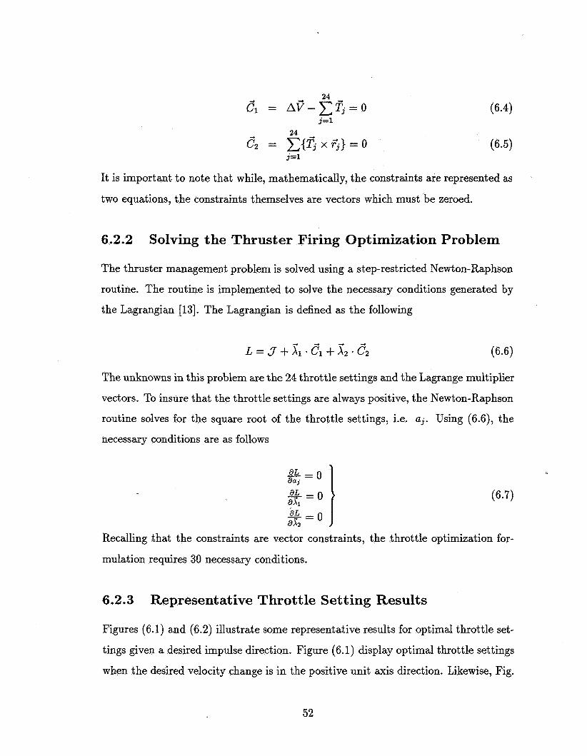
It is important to note that while, mathematically, the constraints are represented as
two equations, the constraints themselves are vectors which must be zeroed.
6.2.2 Solving the Thruster Firing Optimization Problem
The thruster management problem is solved using a step-restricted Newton-Raphson
routine. The routine is implemented to solve the necessary conditions generated by
the Lagrangian [13]. The Lagrangian is defined as the following
The unknowns in this problem are the 24 throttle settings and the Lagrange multiplier
vectors. To insure that the throttle settings are always positive, the Newton-Raphson
routine solves for the square root of the throttle settings, i.e. aj. Using (6.6), the
necessary conditions are as follows
Recalling that the constraints are vector constraints, the throttle optimization for-
mulation requires 30 necessary conditions.
6.2.3 Representative Throttle Setting Results
Figures (6.1) and (6.2) illustrate some representative results for optimal throttle set-
tings given a desired impulse direction. Figure (6.1) display optimal throttle settings
when the desired velocity change is in the positive unit axis direction. Likewise, Fig.
52

(6.2) display optimal throttle settings when the desired velocity change is in the nega-
tive unit axis direction. Each individual subplot in the figures represent optimization
results from the step-restricted Newton-Raphson routine.
u) Unit impube in +Y dir&ion Q)
5 10 15 20 25
Thruster number
Figure 6.1: Optimal throttle settings for positive axial direction unit impulses
53

L .- Unit impul% in -X dirdon
(Do.2 -.... .... .. ........ 1 .................. .; ......... .. .. 4 .. ............. : ...........,......- - z 5 10 15 20 2s
! Unit impu$e in -Y dire&ion 11. 1 S I I I I r I
Figure 6.2: Optimal throttle settings for negative axial direction unit impulses
54

Chapter 7
Summary and Recornmendations
This study focused upon the development of an open-loop guidance architecture for
the terminal phase of an autonomous rendezvous and docking (AR&D) mission to
determine the capability of using the Global Positioning System (GPS) for initial rela-
tive position determination instead of conventional optical sensors. The development
of the guidance architecture was performed in two steps. First, feasible command
trajectories were determined for one, two, and three impulse maneuvers. Second, a
thruster management system was developed to execute these command trajectories.
Several assumptions were made concerning the type of terminal phase docking
maneuver. First, the chase vehicle was on-orbit with the target and trailed the target
by a given distance. Second, while at its initial position, the chase vehicle was assumed
to have no relative motion with respect to the target. Third, the docking mechanism
was assumed to be located on the far side of the target vehicle. This required a
docking maneuver where the chase flies to the front of the target to complete the
mission. Finally, relative GPS issues such as integer ambiguity and cycle slip were
assumed to be resolved. In this study, linear time-invariant equations of motions were
used to govern the relative dynamics between the chase and target vehicles.
Previous command trajectory research suggested that docking accuracies were
highly sensitive to initial vertical position errors while fairly insensitive to initial
horizontal position errors of the chase vehicle. In this study, command trajectories
were deemed feasible by maximizing the locus of admissible initial vertical positions
55

and comparing the maximum vertical position error to documented relative GPS
accuracies. In this study, constrained trajectory optimization was used to determine
this locus of initial positions.
Results show that for small initial horizontal separations between the chase and
target vehicles, one impulse command trajectories were not feasible based on required
initial vertical position accuracy. For small separations, the initial vertical position
accuracy were too stringent for relative GPS position determination. The robustness
for two impulse command trajectories were significantly better. The accuracy re-
quired of two impulse command trajectories were determined to clearly be obtainable
using relative GPS. At a given initial horizontal separation, required initial vertical
position accuracies were nearly constant regardless of the application time of the sec-
ond impulse. As compared to two impulse command trajectory results, initial vertical
position accuracy requirements for the three impulse command trajectory exhibited
no significant improvement. However, the increase in total velocity change required
of the chase vehicle was significant to the point where the implementation of a three
impulse maneuver over a two impulse maneuver was not warranted. From an engi-
neering standpoint, the two impulse command trajectory was the best maneuver to
complete the specified docking mission.
The development of the thruster management system was based upon determining
optimal throttle settings given a desired impulse command. In addition to realizing
the impulse command, an additional constraint required that the resultant chase vehi-
cle motion was purely translational. The specific model used for the chase vehicle was
the cargo transfer vehicle. In this study, it was determined that formulations could
be developed where the thruster management system realized the impulse commands
while producing no resultant moment. Research in designing the management system
was preliminary in that no effort was made on developing a modulator to determine
minimum thruster firing times based on the throttle settings.
There are several areas of possible future work in this field. Additional work
is required to complete the thruster management system. Future work could also
involve examining thruster error and finite-burn effects. Additionally, navigational
56

errors and pointing errors are very important with these maneuvers. Thus, future
research could be devoted to these issues. Other areas of recommended research
could involve incorporating other force effect, such as differential drag, gravitational
effect of the Moon, and solar pressure, which can affect the desired motion of the
chase vehicle. Finally, future work could involve developing a closed-loop guidance,
navigation, and control system where navigation corrections are performed by relative
GPS in real-time.
57

Bibliography
[l] Leonard, C. L. and Bergmann, E. V., “A Survey of Rendezvous and Docking
Issues and Developments”, Orbital Mechanics and Mission Design: Advances in
the Astronautical Sciences, Vol. 69, Paper AAS 89-158, April 24-27, 1989, pp.
85-101.
[2] Kunkel, B., Lutz, R., and Manhart, S., “Advanced Opto-electrical Sensors for
Autonomous Rendezvous-Docking and Proximity Operations in Space”, Proceed-
ings Solid State Imagers and Their Applications, Vol. 591, Nov. 26-27, 1985, pp.
138- 148.
[3] Fukase, M., Maruyama, T., Uchiyama, T., Okamoto, O., and Yamaguchi, I., “Visual Sensing for Autonomous Rendezvous and Docking”, 4 1 st Congress of
the International Astronautical Federation, Oct. 6-12, 1990.
[4] Curtis, A., ed., Space Satellite Handbook, 3rd Edition, Gulf Publishing Company,
1994, pp. 86-87, 114-115.
[5] Green, G. B., Massatt, P. D., and Rhodus, N. W.,“The GPS 21 Primary Satellite
Constellation”, Navigation: Journal of the Institute of Navigation, Vol. 36, No.
1, Spring 1989, pp. 9-24.
[6] Upadhyay, T., Cotterill, S., and Deaton, A. W., “Autonomous Reconfigurable
GPS/INS Navigation and Pointing System for Rendezvous and Docking”, AIAA
Space Programs and Technologies Conference, March 24-27, 1992.
171 Hohwiesner, B. and Pairot, J., “On-Orbit Demonstration of Automated Clo-
sure and Capture Using European & NASA Proximity Operations Technologies
58

and an Existing, Serviceable NASA Explorer Platform Spacecraft”, AIAA Space
Programs and Technologies Conference, March 24-27, 1992.
Smith, A., Hesper, E., Kuijper, D., Mets, G., Ambrosius, B., and Wakker, K.,
“TOPEX/Poseidon Precise Orbit Determination”, SpacefEight Mechanics 1994,
Vol. 87, Part 11, Paper AAS 94-137, 1994, pp. 1107-1124.
Euler, H., “Achieving High- Accuracy Relative Positioning in Real-time: System
Design, Performance and Real-time Results”, 1994 IEEE Position Location and
Navigation Symposium, April 11-15, 1994, pp. 540-546.
[lo] DiPrinzio, M.D. and Tolson, R.H., “Evaluation of GPS Position and Attitude
Determination for Automated Rendezvous and Docking Missions”, NASA Con-
tractor Report 461.4, July 1994.
[ll] Mullin, L.D., “Initial Value and TPBV Solutions to the Clohessy-Wiltshire Equa-
tions”, The Journal of Astronautical Sciences, Vol. 40, No. 4, 0ct.-Dec. 1992,
pp. 487-501.
[12] Burden, R. L. and Faires, J. D., Numerical Analysis, Fifth Edition, PWS-Kent
Publishing Company, 1993, pp. 98-105.
1131 Bryson, A. E. and Ho, Y . , Applied Optimal Control: Optimization, Estimation,
and Control, Hemisphere Publishing Corporation, 1975.
59

Appendix A
Early AR&D Formulations
The optimization formulations and results presented in this appendix illustrate early,
unpublished AR&D research performed by Dr. Daniel D. Moerder (NASA LaRC) and
Dr. Robert B. Bless (Lockheed). The basic research involves determining optimized
trajectories for a single impulse command trajectory with no preconceptions about
the initial position error sensitivities in relation to docking accuracies. Thus, their
formulations involve determining a locus of initial positions, xo and yo, and not just
a locus of initial vertical positions. Within this locus, the chase vehicle performs a
fixed sequence of impulses which translates the vehicle into the target while satisfying
the accuracy requirements listed in Table (2.1).
A.1 Early AR&D Problem Statement
An early approach to this problem is to determine the maximum two-dimensional
“footprint” of admissible initial positions for the chase vehicle such that a single fixed
impulse anywhere within this footprint results in a successful docking with the target.
60

In polar coordinates, the formulation is to maximize
3 = xi + yi = ro 2
where the initial position is represented as
xo = rocos8
yo = rosin8
To generate a footprint of admissible initial positions, the parameter 8 is allowed to
range from 0 deg to 360 deg. In this approach, the only constraints to the optimization
problem are to satisfy the target conditions summarized in Table (2.1) and represented
mathematically in Eqn. (2.4).
A.2 Early AR&D Results
Figure (A.1) illustrate admissible position errors about the nominal initial chase vehi-
cle position, xo and yo, which in this figure is centered about the origin. These AR&D
results show that to meet the accuracy required at docking the position errors of the
chase vehicle at its initial condition are very sensitive to the initial vertical position
errors while fairly insensitive to horizontal position errors. In fact, the admissible
errors in the horizontal position of the chase vehicle are in the order-of-magnitude
of several feet. Documented results of relative GPS orbit determination performance
has demonstrated that local horizontal position errors of several feet are clearly ob-
tainable [8, 9, 101. However, based purely on these results, it is uncertain whether
the admissible errors in the initial vertical position of the chase vehicle is attainable
through relative GPS position determination.
It is important to point out that this early AR&D formulation is based on the
assumption that intermediate trajectories within the boundary of the footprint satisfy
target constraints. However, results from Chapter 3 show that this assumption is not
true without actually constraining the interior trajectories. Thus, if interior trajectory
constraints are included in the formulation, the overall magnitude of the footprint
61

15 I 1 I I I I I I
J -1 5 -1 0 -5 0 5 10 15
Horizontal initial position enor (ft) -1 5’
Figure A.l: Early AR&D footprint results of admissible position errors at the chase
vehicle initial condition
would decrease, but it is safe to presume that the trend exhibited in Fig. (A.l) would
continue to exist.
Furthermore, optimized trajectory simulations of this single impulse AR&D ma-
neuver are performed based on the optimization formulation of Eqns. (A.l) and
(2.4). Figure (A.2) illustrate two chase vehicle trajectories initiated from the upper-
most and lowermost admissible vertical positions. Based on Fig. (A.2), the chase
vehicle approaches the target vehicle tangentially from either side. In this basic for-
mulation, the final approach trajectory of the chase vehicle is uncontrolled. Ideally, it
is best to formulate the trajectory optimization problem such that the chase vehicle
always approaches the target from a specified direction. As seen in Fig. (A.2), to
accommodate different chase vehicle approach trajectories, the target vehicle docking
port would have to be continually reorientated based upon the initial position of the
chase vehicle. While reorientating small target vehicles would certainly be possible,
this scenario is impractical for large proposed target structures such as Space Station
Freedom.
62

0 Relative position x (ft)
Figure A.2: Early AR&D trajectory simulation starting from the extreme ends of
admissible initial vertical chase positions
The results of this early AR&D formulation lay the groundwork for the current
constrained trajectory optimization problem presented in Chapter 3. It hints at the
need to maximize a locus of initial vertical positions for the chase vehicle. It also
illustrates the required addition of gate constraints that must be satisfied by the chase
vehicle to generate more direct and predictable optimized approach trajectories.
63

Appendix B
Quadratic Behavior at Target
Vehicle
Analysis of rendezvous and docking results has shown that Eqn. (3.5) is violated for
the intervals of yo - AyO 5 yo 5 yo + Ayo at a given 20. To adequately satisfy this
constraint, an assumed parabolic behavior of ey is exploited by modeling the behavior
of Eqn. (3.5) as a quadratic according to Eqn. (3.16). The additional constraint
expression of Eqn. (3.18) is required in the three trajectory problem formulation.
There are two governing equations related to the behavior of yf. By the Clohessy-
Wiltshire dynamical model [ll], they are
4 sin wt 2YO "(yo, t ) = xo + Gyo(wt - sinwt) + io( - 3t) + -(1 - coswt) (B.1) W W
2i0 YO Y(Yo,t) = (4 - COS wt)yo - -(I W - coswt) + - w sinwt
where 20, io, and $0 are assumed to be given for a particular command trajectory.
To show quadratic behavior, Eqns. (B.l) and (B.2) are expanded about the target,
i.e. at t = tf , using a first-order Taylor series. The Taylor series will have the form:
64

where, at the target, Sxf = 0. Note that the higher-order terms in Eqns. (B.3) and
(B.4) are negligible since secular terms exist in the governing equations.
From Eqn. (B.3), a set of all feasible solutions of Stf in terms of Syo is found to
be
(B.5) 6(sin wtf - wtf)
6wy0( 1 - cos wtf) - i0(3 - 4 cos wtf) + 2y0 sin wtf
Using Eqns. (B.4) and (B.5), a perturbation relation between Syf and Syo is found
Stf = SYO
to be of the form:
where
(B-7) 1 A = 6w(7 - 7 cos wtf - 3wtf sin wtf)
B = io(12wtf sin wtj + 25 cos utj - 24) + yo(8 sin wtf - 6wtf cos utj)
C = 6w( 1 - COS wtf)
D = i0(4coswtf - 3) + 2$0 sinwtf
Recall that Eqn. (B.7) contains xo, 20, and yo which are assumed to be given for a
particulas impulse scheme.
Clearly, the perturbation relation of Eqn. (B.6) represent the tangential relation-
ship between the final position of the chase vehicle, yf, in terms of its initial position,
yo. To show a relation is quadratic with a clear maximum point is the equivalent
to showing that the corresponding tangential relation is linear. The relation derived
using perturbation methods is a ratio of linear relations for all feasible solutions of
tf and yo. However, results for the impulse command trajectories posed in this work
consist of a specific set of feasible solutions. Thus, to show that Eqn. (B.6) is linear,
the magnitude of A must dominate,the magnitude of C. Evaluating Eqn. (B.7) using
65

optimized single impulse solutions 'at xo = 600 f t results in the following order of
magnitudes:
B M 10-1
c M 10-5
D x
Based on Eqn. (B.8), the dominant linear relation in Eqn. (B.6) is the numerator.
The dominant term in the denominator of Eqn. (B.6) is the stand-alone constant D.
In fact, the smallest order of magnitude in Eqn. (B.8) is the one associated with the
linear coefficient term in the denominator. At O(lO-'), this term is three orders-of-
magnitude smaller than the magnitude of A which clearly implies that Eqn. (B.6)
can be approximated as a linear relation. Figure (B.l) displays Eqn. (B.6) using
results from the optimized single impulse command trajectory over the entire interval
of yo and its corresponding set of t f . The graphic shows a decreasing linear relation
crossing the zero axis. This shows fairly conclusively that yf(y0) is a parabolic relation
with a clear maximum.
66

-9.8 -9.6 -9.4 -9.2 , -9 -8.8 initial vettical position, yo (in)
Figure B. 1: Perturbation results of 2 using optimized single-impulse results at
~0=600 ft
67

An Open Loop Guidance Architecture For Navigationally Robust On-orbii Docking
6. AUlHOCyS)
Hung-Sheng Chern
NCC1-104
WU 242-80-01 -02
The George Washington University Joint Institute for Advancement of Flight Sciences
Langley Research Center NASA CR-4687 Hampton, VA 23681 -0001
The development of an open-loop guidance architecture is outlined for autonomous rendezvous and docking (AR&D) missions to determine whether the Global Positioning System (GPS) can be used in place of optical
1 sensors for relative initial position determination of the chase vehicle. Feasible command trajectories for one, two, and three impulse AR&D maneuvers are determined using constrained trajectory optimization. Early AR&D
1 command trajectory results suggest that docking accuracies are most sensitive to vertical position errors at the initial conduction of the chase vehicle. Thus, a feasible command trajectory is based on maximizing the size of
1 the locus of initial vertical positions for which a fied sequence of impulses will translate the chase vehicle into 1 the target while satisfying docking accuracy requirements. Documented accuracies are used to determine whether relative GPS can achieve the vertical position error requirements of the impulsive command trajectories. Preliminary development of a thruster management system for the Cargo Transfer Vehicle (CTV) based on optimal throttle settings is presented to complete the guidance architecture. Results show that a guidance architecture based on a two impulse manuever generated the best performance in terms of initial position error and total velocity change for the chase vehicle.
14. SUBJECT TERMS 115. NUMBER OF PAGES
Rendezvous and Docking, On-otbii Maneuvers, Space Vehicle Guidance
I 17. SECURITY CLASSIFICATION 18. SECURITY CLASSIFICATION 19. SECURITY CLASSIFICATION 20. LIMITATION OF ABSTRACT
OF REPORT OF THIS PAGE OF ABSTRACT
unclassified unclassified
Standard Form 298 (Rev. 2-89) Pfescnbsd ty ANSI Std. 239-18 298-102
NSN 7540-01-280-5500