(NASA-CR-U20736) HORKING EODEL OF THE N75-21562LONDON HO-ENT READOUT SYSTEH SemiannualProgress Report, 1 Jan. -30 Jun. 1974(Alabama Univ.o Huntsville.), 38 p HC $3.75 Unclas

CSCL 13K G3/34 19247

WORKING MODEL

OF THE

LONDON MOMENT READOUT SYSTEM

January 1, 1974 - June 30, 1974

John Benjamin Hendricks

and

Gerald R. Karr

The University of Alabama in Huntsville

School of Graduate Studies and Research

Huntsville, Alabama 35807

SEMI-ANNUAL PROGRESS REPORT

Contract Number NAS8-29316

/'q

Prepared for

George C. Marshall Space Flight CenterNational Aeronautics and Space Administration

Marshall Space Flight Center, Alabama 35812

March 1975

https://ntrs.nasa.gov/search.jsp?R=19750013490 2020-04-03T04:04:04+00:00Z

I. PROGRESS ON STUDY PROGRAM

This progress report covers the work done by Dr. Karr on the theory

of super fluid plug operation. The purpose of the work was to develop

expressions which explain the behavior of the super fluid plug which is

being proposed for use in liquid helium management in space for the

relativity experiment.

The details of the calculations and results are provided in the

appendix. In summary, the essential results are that the mass flow rate,

i, through the plug is given by the expression

P (T) + Phm v h

AT pSL2 1K + F IA*

where AT is the total area of the plug, p is the density, S is the en-

tropy, L is the latent heat of vaporization, and K is the total thermal

conductivity of the plug with the liquid helium included. All properties

are for the helium in the liquid state evaluated at the temperature on

FAthe liquid side of the plug. The factor A is related to the im-

pedance of the pumping system on the gas side of the plug.

Solution was also obtained for the mass flow at temperature above

the lambda point temperature given by

fn Pv (T) + Ph

_A14r

2

where 4 is the viscosity, k is the permeability of the plug and A is

the total area of pores contained in a cross section of the plug. The

value of A is found from measurement of the plug porosity.

Solutions were obtained for the normal and superfluid velocity

(equation 29 and 30 of the appendix). This was done in order to inves-

tigate the possibility of the superfluid component reaching the critical

velocity, thereby violating certain assumptions in the derivation. We

found that for the plugs of pore sizes under consideration here, that

the superfluid velocity is always less than the critical velocity. We

also conclude that only for pore sizes larger than 10 micron would this

effect become of importance.

A brief comparison of the theory results with the experimental re-

sults obtained by Dr. Urban are made. We find that the theory is very

accurate in the region of 1.50K but departs as much as 30% at near 20K.

The source of error is believed to be the approximate linear relationship

used to represent the pumping system impedance.

II. PLANS FOR NEXT REPORTING PERIOD

The next semi-annual progress report will cover work on the magne-

tometer and low temperature research apparatus by Dr. Hendricks and work

on magnetic shielding calculations.

Jo B. Hendricksincipal Investigator

Gerald R. KarrPrincipal Investigator

asw

APPENDIX

THEORY OF SUPER FLUID PLUG OPERATION

by

Gerald R. Karr

I. INTRODUCTION

The operating characteristics of a porous plug which has liquid

helium on one side and which is pumped on under vacuum on the other

side is discussed. Such a device has application to the containment

of liquid helium in a zero gravity environment. The plug has the capa-

bility of acting as a phase separator and, to some extent, as a temperature

control device.

The system to be considered in the work consists of a container of

liquid helium which is well isolated. The only means for mass flow out

of the container is through a plug mode of porous material. The plug

is assumed to have liquid helium on the container side while the other

side of the plug is evacuated. In the experiment ran on earth under

one g, the plug is situated on the bottom of the container. The physical

system employed in the evacuation is found to be important to the plug

operation. Three cases in particular will be considered: (1) perfect

evacuation with zero pressure, (2) evacuation through an chocked orifice,

and (3) evacuation through a long, small diameter pipe with heating.

The last case is the one most likely to occur in practice.

Two distinct ranges of temperature operation are of importance in

describing plug flow. (1) Above T = 2.1720K and (2) Blow T = 2.1720K.

The temperature 2.1720K is the point at which liquid helium changes from

Hel which exists at the higher temperature range to a second liquid

5

phase Hell at the lower range of temperature. Hel is a normal liquid

phase and the flow of this liquid is described by classical fluid flow

relationships. In the Hell phase, however, the fluid exhibits super

fluid properties which must be taken into consideration.

For purposes of describing the plug operation, the two-fluid model

of the Hell phase is used. The two-fluid model considers Hell to consist

of a super fluid component, ps, and a normal fluid component, pn, where

the total density of the fluid, p, is given by

P = Ps + Pn

The ratio pn/p drops from a value of one at the X-point and asymptoticly

approaches zero at OOK.

The fluid flow of Hell using the two-fluid model is described by

the following set of Landau's equations (see for example R. J. Donnelly,

Experimental Superfluidity, University of Chicago Press, 1967),

avs PS PnPs 2

P + Ps ( v s Vp + P ST + - V (n-vs) (1)

avn PnPn -a + P (v.n V) v n Vp - ps SVT

PnPs 2 2- V (v n v ) + t V v (2)

The first term on the right hand side represents the reaction of the

fluid to pressure forces, the second term is associated with the thermo-

mechanical effect, and the third term is a mutual friction dependent on

the motion of one component with respect to the other, Equation (2)

contains a fourth term on the right hand side which represents the

effect of viscosity. The flow equation for temperature above the X

point can be obtained from equation (2) for the case of ps = 0 and

Pn =P

The flow equations are found to reduce considerably for the com-

bination of steady state flow and small VT across the plug. These

conditions are reasonable assumptions for plugs made with large pore

(5-10p) material. For small pore material (.54), the VT across the

plug is found to be large. Also, small pore materials seem to exhibit

time dependent behavior which may require non-steady state analysis.

In summary, the description of porous plug operation for liquid

helium management is divided into the following items of importance.

1. Type of evacuation

a. perfect vacuum

b. through orifice

c. through pipe with heating

2. Temperature range

a. above X-point

b. below -point

3. Simplifying assumptions

a. steady state

b. small VT

4. Velocity range of superfluid

a. less than critical velocity

b. greater than critical velocity

7

This report will consider the special case of small VT, steady

state operation of a plug evacuated through an ideal orifice over the

full temperature range. The results will be reducable to the case of

a perfect vacuum evacuation. Future progress reports will consider the

case of evacuation through a pipe with heating and large VT across the

plug.

II. SMALL VT WITH EVACUATION THROUGH CHOKED ORIFICE

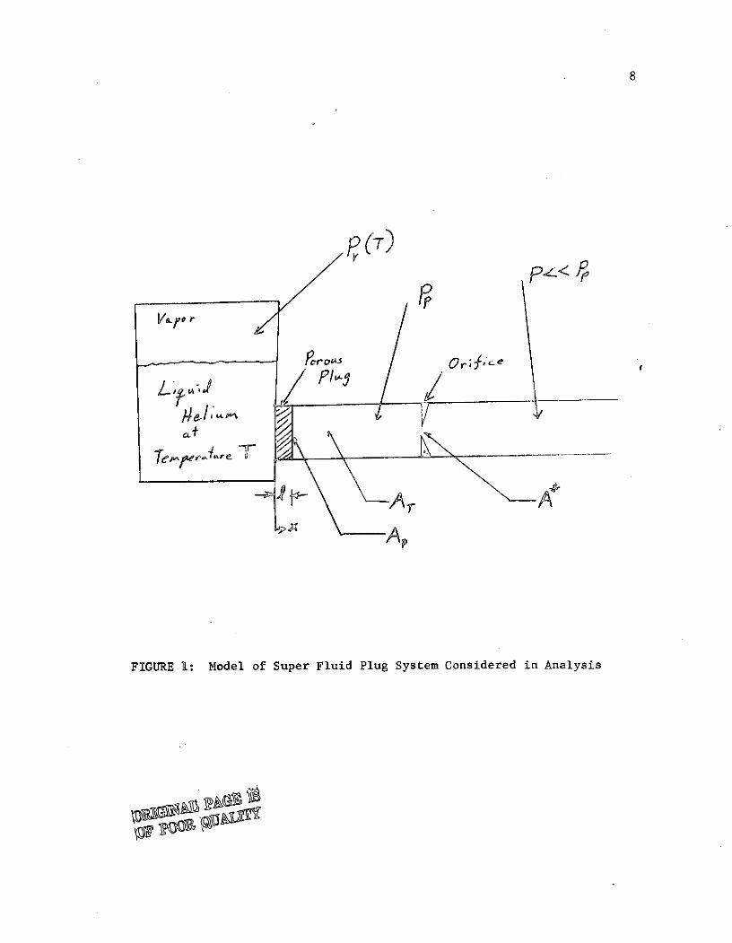
The model of the system to be described is shown in Figure 1. The

flow through the orifice is linear in the pressure difference across the

orifice. If the pressure downstream of the orifice is small compared

to the pressure in the plenum, Pp, the mass flow per unit area through

the orifice is given by

it/A* = F P (3)p

where m is the mass flow rate, A is a flow area at the point that Mach

Number M=l, and F is given for a choked orifice by

F=C 2 y-1 (4)w RT y+l

where C is a orifice discharge coefficient, y is the ratio of specific

heats, R is the gas constant of the gas and T is the temperature of

the gas in the plenum. For pressure ratios acorss the orifice of .1

or less, the value of C is 0.85.

In normal operation, heat is transferred out of the container

through the plug at a rate proportional to the conductivity across the

plug. The heat comes from heat leaks into the container due to imperfect

a + i

Ar~A

FIGURE 1: Model of Super Fluid Plug System Considered in Analysis

9

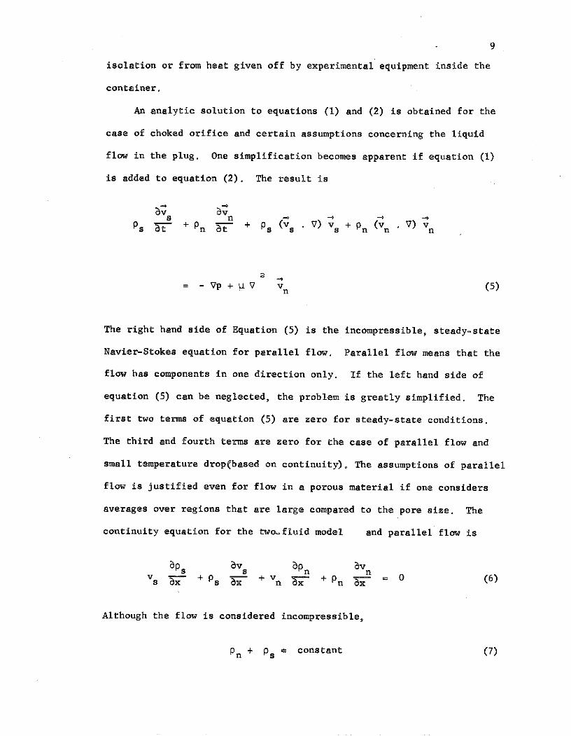
isolation or from heat given off by experimental equipment inside the

container.

An analytic solution to equations (1) and (2) is obtained for the

case of choked orifice and certain assumptions concerning the liquid

flow in the plug. One simplification becomes apparent if equation (1)

is added to equation (2). The result is

-4

by avs n -PPSV + Pn + P (v s V) Vs + p n (v ) n

= -Vp + ~ V Vn (5)

The right hand side of Equation (5) is the incompressible, steady-state

Navier-Stokes equation for parallel flow. Parallel flow means that the

flow has components in one direction only. If the left hand side of

equation (5) can be neglected, the problem is greatly simplified. The

first two terms of equation (5) are zero for steady-state conditions.

The third and fourth terms are zero for the case of parallel flow and

small temperature drop(based on continuity). The assumptions of parallel

flow is justified even for flow in a porous material if one considers

averages over regions that are large compared to the pore size. The

continuity equation for the two-fluid model and parallel flow is

ap y ap avs s Pn n

s x + P x +n +n x - 0 (6)

Although the flow is considered incompressible,

Pn + Ps a constant (7)

10

the individual densities are a strong function of temperature as

discussed earlier. For this reason, the derivatives of ps and p n

may be finite if a temperature gradient exists. Since heat transfer

is taking place, one can neglect these derivatives only if the tempera-

ture gradient is small enough to make the resultant density gradient

negligible. This condition can be met for plugs with large pores

except near TX where the density changes are large with respect to

temperature. The large pore plugs have a high effective thermal con-

ductivity and therefore a small gradient of temperature as will be

discussed later.

Under the assumption of small AT and parallel flow, equation (5)

becomes

2

Vp PV vn (8)

where the velocity vn is determined completely by the pressure drop.

If the plug were constructed of smooth channels, such as a bundle of

capillary tubes of radius R, the exact solution to the above for laminar

pipe flow could be employed to find the volume flow rate given by

4

2= R d(9)n 8p dx

which shows that the flow rate is a linear function of the pressure

drop. The plugs being considered by NASA at this time, however, are

made of packed granular material which cannot be considered to have

smooth passages.

For flow through porous material, a relationship similar to

equation (9) is available given by Darey's law (see Muskat, Flow of

Homogeneous Puuido)

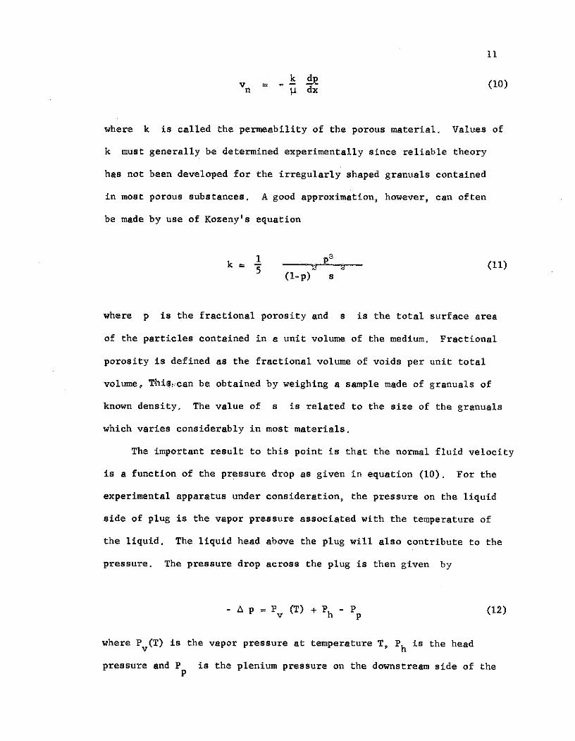
v k d (10)n = dx

where k is called the permeability of the porous material. Values of

k must generally be determined experimentally since reliable theory

has not been developed for the irregularly shaped granuals contained

in most porous substances. A good approximation, however, can often

be made by use of Kozeny's equation

1 pk = (11)(l-p) s

where p is the fractional porosity and s is the total surface area

of the particles contained in a unit volume of the medium. Fractional

porosity is defined as the fractional volume of voids per unit total

volume, Thie@can be obtained by weighing a sample made of granuals of

known density. The value of s is related to the size of the granuals

which varies considerably in most materials.

The important result to this point is that the normal fluid velocity

is a function of the pressure drop as given in equation (10). For the

experimental apparatus under consideration, the pressure on the liquid

side of plug is the vapor pressure associated with the temperature of

the liquid. The liquid head above the plug will also contribute to the

pressure. The pressure drop across the plug is then given by

- A p = P (T) + Ph - Pp (12)

where P (T) is the vapor pressure at temperature T, Ph is the head

pressure and P is the plenium pressure on the downstream side of thep

12

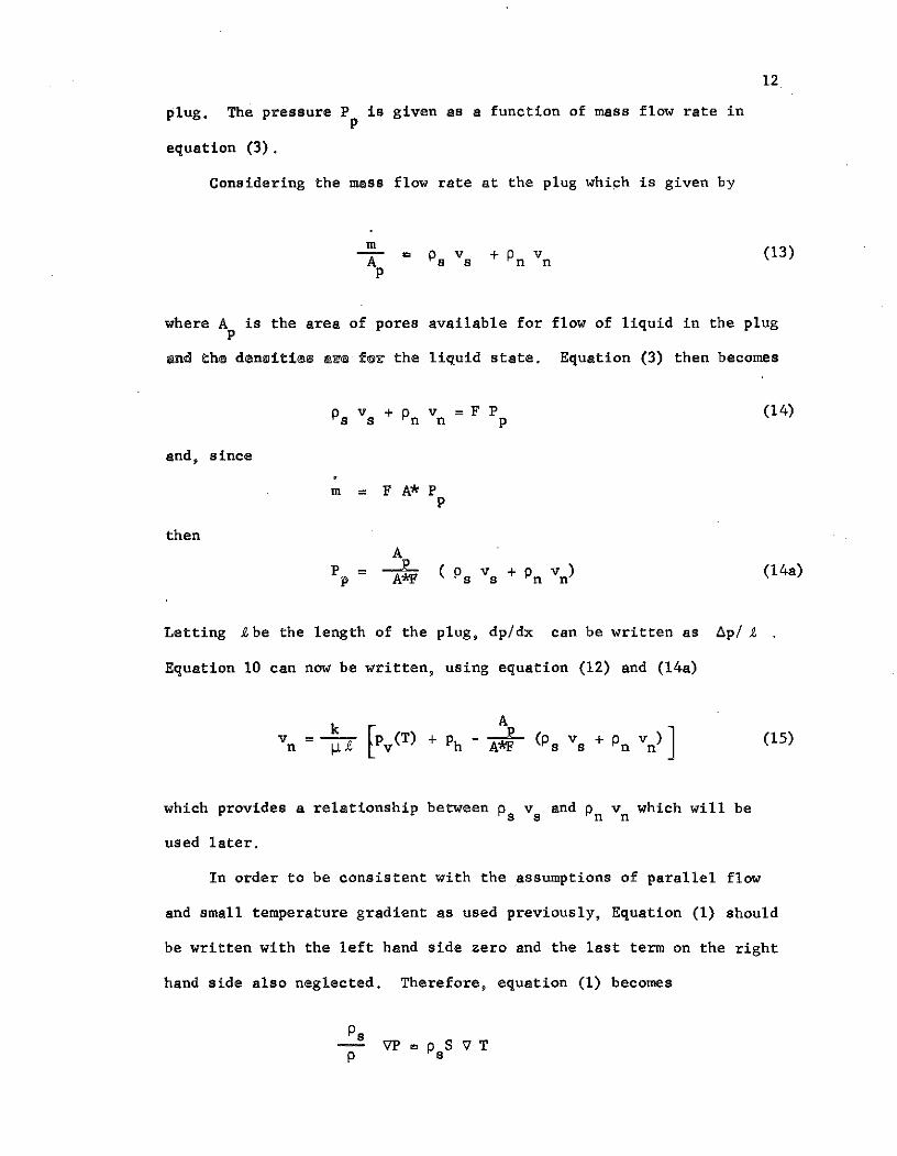
plug. The pressure P is given as a function of mass flow rate in

equation (3).

Considering the mass flow rate at the plug which is given by

m 5 v + P v (13)A s + n nP

where A is the area of pores available for flow of liquid in the plug

and the densities are for the liquid state. Equation (3) then becomes

P vs + n v = F P (14)

and, since

m = F A* Pp

thenA

P -- R- ( P v + Pn ) (14a)p A*F s s n n

Letting lbe the length of the plug, dp/dx can be written as Ap/ Y

Equation 10 can now be written, using equation (12) and (14a)

AVn v ( T ) + Ph - (s + v)] (15)

which provides a relationship between ps vs and pn vn which will be

used later.

In order to be consistent with the assumptions of parallel flow

and small temperature gradient as used previously, Equation (1) should

be written with the left hand side zero and the last term on the right

hand side also neglected. Therefore, equation (1) becomes

- VP f psS VTP s

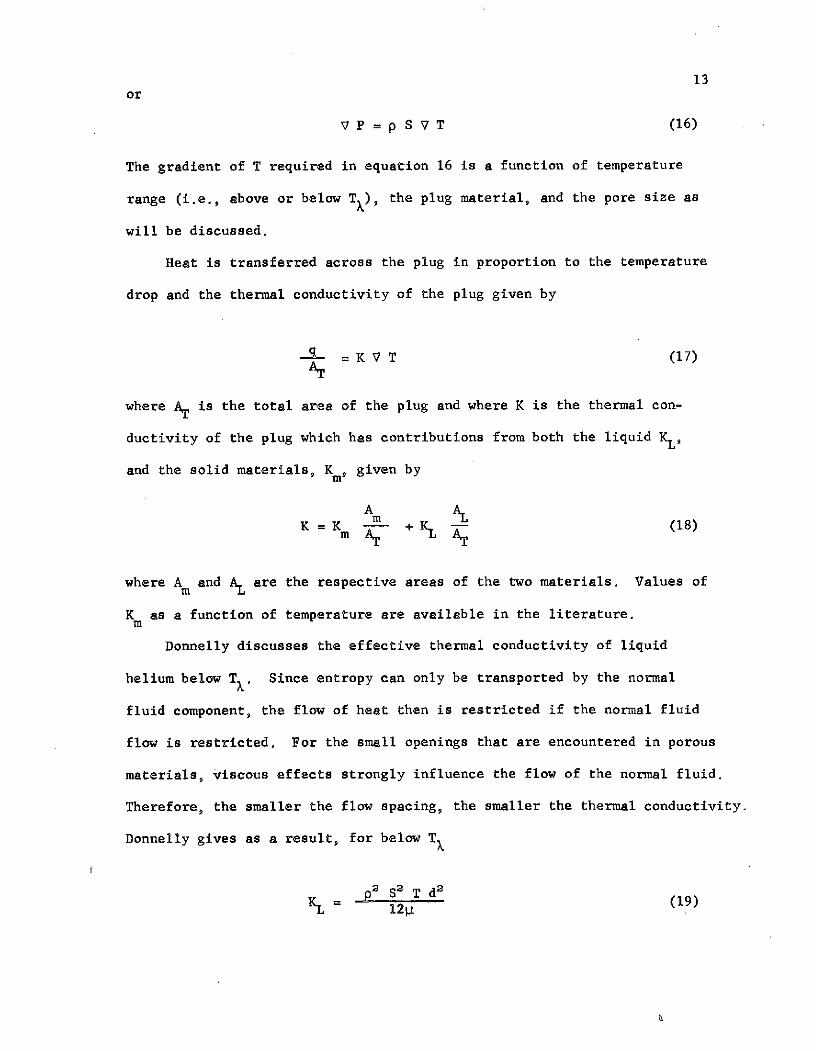
13or

V P = p S V T (16)

The gradient of T required in equation 16 is a function of temperature

range (i.e., above or below Tx), the plug material, and the pore size as

will be discussed.

Heat is transferred across the plug in proportion to the temperature

drop and the thermal conductivity of the plug given by

- K V T (17)AT

where AT is the total area of the plug and where K is the thermal con-

ductivity of the plug which has contributions from both the liquid KL,

and the solid materials, K , given by

A ALK = K + KL (18)

mAT

where A and AL are the respective areas of the two materials. Values of

K as a function of temperature are available in the literature.m

Donnelly discusses the effective thermal conductivity of liquid

helium below T . Since entropy can only be transported by the normal

fluid component, the flow of heat then is restricted if the normal fluid

flow is restricted. For the small openings that are encountered in porous

materials, viscous effects strongly influence the flow of the normal fluid.

Therefore, the smaller the flow spacing, the smaller the thermal conductivity.

Donnelly gives as a result, for below T

P2 S2 T d2KL 12 - (19)

14

'where S is the entropy. Since S is a strong function of temperature,

KL, also becomes a strong function of temperature as evidenced by the

approximation

KL 1.2 x 105 T12 .2 d2 (20)

Heat conductivity of helium at 3.30 k is only

KL (3.30 k) = 6 x 105 cal/deg/cm/sec (21)

Large pore size then results in extremely high thermal conductivities

below TX which tends to be the dominant term in equation 18.

The heat that is transferred across the plug is liberated in

transforming the liquid into a gas at the surface of the plug. The heat

flow then is related to the mass flow rate and the latent heat of vapori-

zation, L, of the helium given by

- L (22)AT AT

Equating the heat flow expression from equation (17) and (22), we obtain

K VT = L (23)

Substituting for VT in equation (16) using the above we get

VP = pS ( ) (24)Usin tion (12and(13 and (14) in e tion (24)

Using equation (12) and (13), and (14) in equation (24)

15

Ap (T) +Ph " (PP vs + P Vn) : A

S h =(Ps s +p S (P v + p ) _v

(25)

This equation is solved for i directly

. P (T) + Phv

(26)AT R2 + 1

K FA*

T'

Equation (26) gives the flow rate through the plug as a function of

temperature of the liquid helium. These results are not the same as

obtained by Selzer, Fairbank, and Everett given by

APKn- pL (27)

pSL

Equation (26) is seen to reduce to equation (27) for the special case

of 1/F = 0 which corresponds to the case of zero pressure on the down-

stream side of the plug. Zero pressure is, however, an unrealistic

assumption for laboratory systems. (A factor of length, £/A, is

evidently missing from equation (27)).

CRITICAL VELOCITY LIMITING

Equation (26) applies only for superfluid velocities below the

critical velocity. In order to assess the M&.idity of this solution,

the superfluid velocity, vs, must be obtained to compare with the critical

velocity, vc. If the critical velocity is reached, another method of

solution must be employed.

In order to obtain a solution for v and v n, equations (26) and

equation (15) are solved simultaneously. Substituting for h/AT from

16

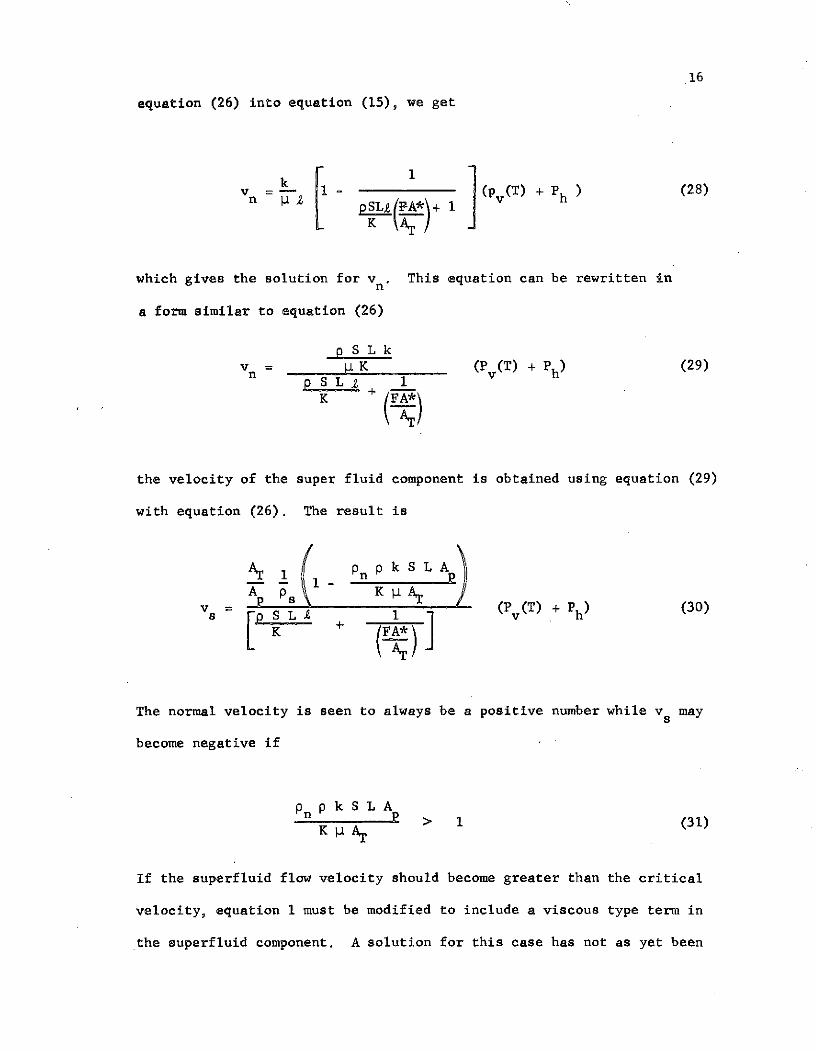
equation (26) into equation (15), we get

vn ~ SLk - A+ I1 (p (T) + P ) (28)

which gives the solution for vn. This equation can be rewritten in

a form similar to equation (26)

p SLkVn 1 K (P (T) + Ph) (29)

pSL£ 1K FA*)

the velocity of the super fluid component is obtained using equation (29)

with equation (26). The result is

AT1 PnpkSLA>I I-

vsS K (Pv(T) + Ph) (30)

The normal velocity is seen to always be a positive number while vs may

become negative if

p pkSLAn p > 1 (31)K p AT

If the superfluid flow velocity should become greater than the critical

velocity, equation 1 must be modified to include a viscous type term in

the superfluid component. A solution for this case has not as yet been

17

developed since it was found that for the pore sizes and pressures under

consideration, critical velocity was not reached. Critical velocity

would be expected to become important, however, for larger sizes of

pores and much higher pressure heads.

ABOVE T

The flow rate above the transition temperature consists of only

the normal fluid which is governed by Darey's law as mentioned earlier.

The flow is still effected by the orifice,however. Equation (12) for the

pressure drop remains the same @nd equation (14) becomes, for flow of

vapor,

F P - (32)p A*

Using equation (10) and (12) with the above we get

AP = --- (p v)p A*F

SApv (P(T) + v) (33)P I v h A*F

where p is the density of the liquid helium.

Solving for p , the flow above TX is given by

Above T% results

Pv(T) + Ph (34)

pAT 1

pr --A T

18

SUMMARY OF BELOW TX RESULTS

Below T

A P (T) + P

(* (26)AT(Ps Vs + Pn Vn) -A T 1K IK FA*\

where

pSL ek

v n P K (Pv(T) + Ph) (29)

K (FA*

and

S 1 P(30)

vs = p S L 1 (Pv(T) + Ph )

K FA*

ATa

19

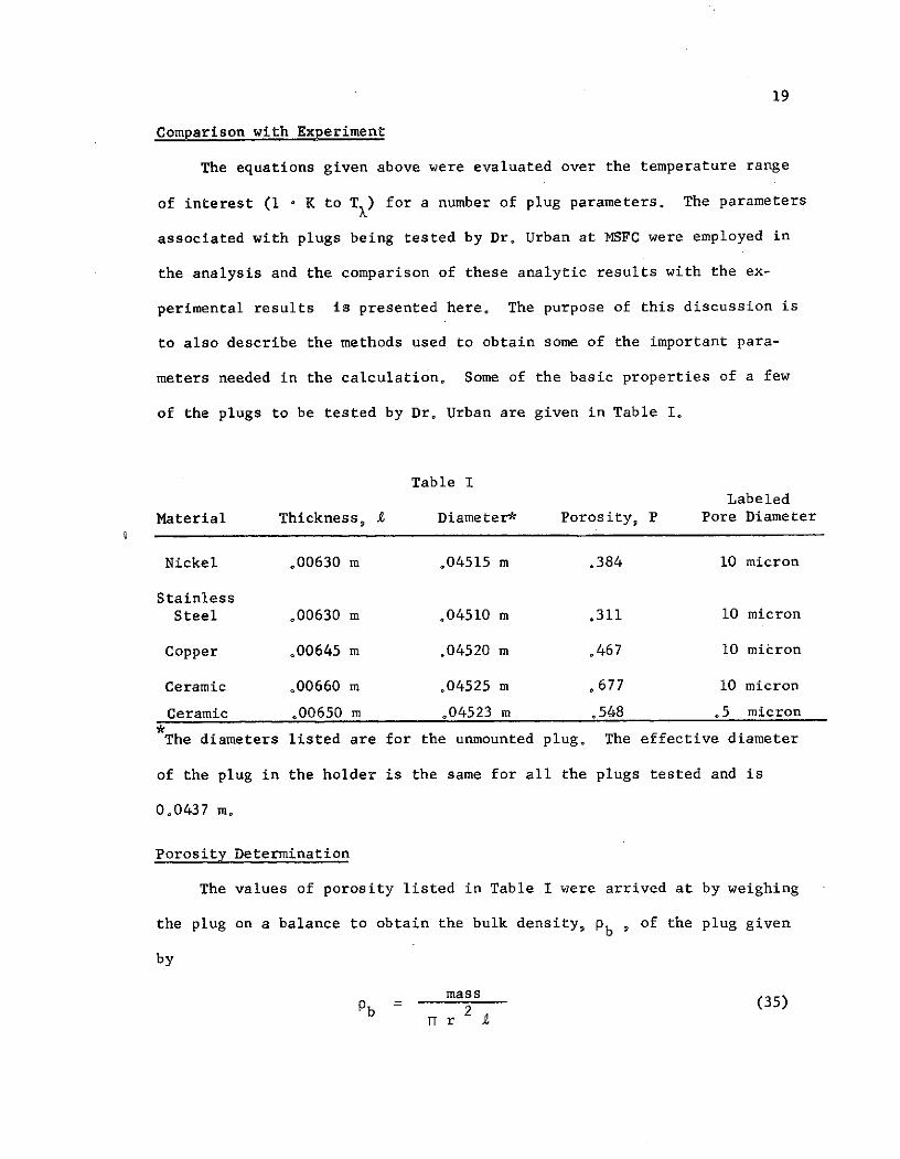
Comparison with Experiment

The equations given above were evaluated over the temperature range

of interest (1 - K to Tx) for a number of plug parameters. The parameters

associated with plugs being tested by Dr. Urban at MSFC were employed in

the analysis and the comparison of these analytic results with the ex-

perimental results is presented here. The purpose of this discussion is

to also describe the methods used to obtain some of the important para-

meters needed in the calculation. Some of the basic properties of a few

of the plugs to be tested by Dr. Urban are given in Table I.

Table ILabeled

Material Thickness, e Diameter* Porosity, P Pore Diameter

Nickel .00630 m .04515 m .384 10 micron

StainlessSteel .00630 m .04510 m .311 10 micron

Copper .00645 m .04520 m .467 10 micron

Ceramic .00660 m .04525 m .677 10 micron

Ceramic .00650 m .04523 m .548 .5 micron

The diameters listed are for the unmounted plug. The effective diameter

of the plug in the holder is the same for all the plugs tested and is

0.0437 m.

Porosity Determination

The values of porosity listed in Table I were arrived at by weighing

the plug on a balance to obtain the bulk density, pb , of the plug given

by

massmass (35)b 2

TTr e

20

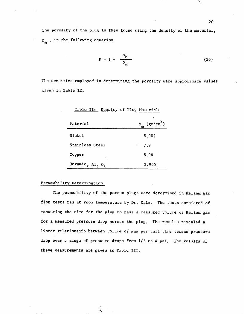
The porosity of the plug is then found using the density of the material,

pm 1 in the following equation

PbP = 1 (36)

The densities employed in determining the porosity were approximate values

given in Table II.

Table II: Density of Plug Materials

Material Om (gm/cm 3 )

Nickel 8.902

Stainless Steel 7.9

Copper 8.96

Ceramic, Al2 03 3.965

Permeability Determination

The permeability of the porous plugs were determined in Helium gas

flow tests ran at room temperature by Dr. Katz. The tests consisted of

measuring the time for the plug to pass a measured volume of Helium gas

for a measured pressure drop across the plug. The results revealed a

linear relationship between volume of gas per unit time versus pressure

drop over a range of pressure drops from 1/2 to 4 psi. The results of

these measurements are given in Table III.

21

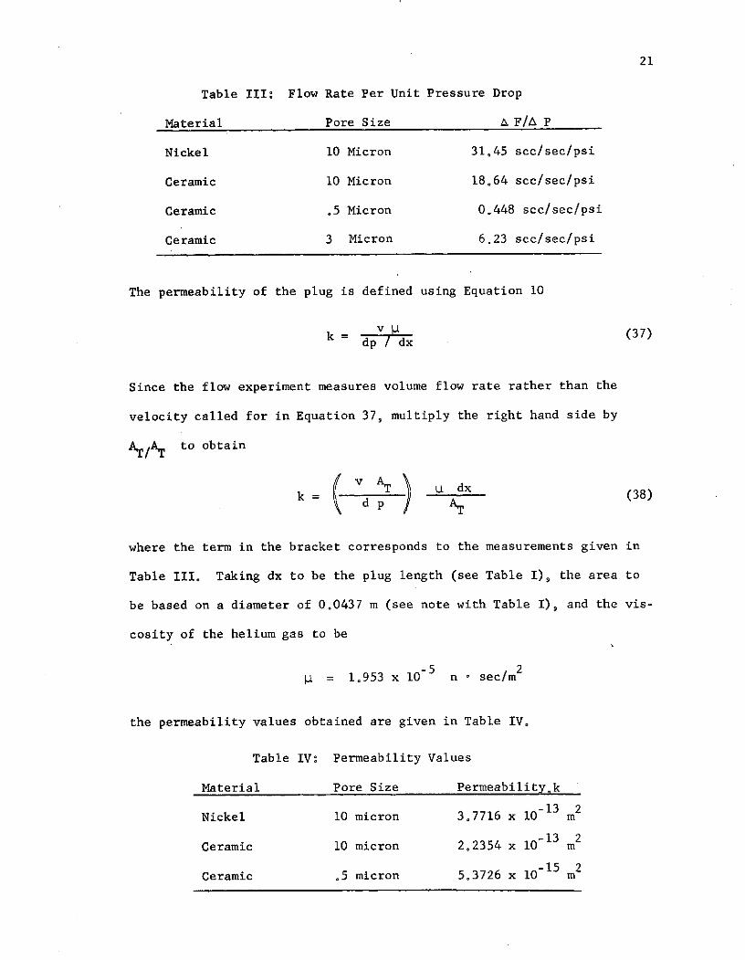
Table III: Flow Rate Per Unit Pressure Drop

Material Pore Size A F/A P

Nickel 10 Micron 31.45 scc/sec/psi

Ceramic 10 Micron 18.64 scc/sec/psi

Ceramic .5 Micron 0.448 scc/sec/psi

Ceramic 3 Micron 6.23 scc/sec/psi

The permeability of the plug is defined using Equation 10

k v L (37)dp / dx

Since the flow experiment measures volume flow rate rather than the

velocity called for in Equation 37, multiply the right hand side by

AT/AT to obtain

k v AT dx (38)dk=p

where the term in the bracket corresponds to the measurements given in

Table III. Taking dx to be the plug length (see Table I), the area to

be based on a diameter of 0.0437 m (see note with Table I), and the vis-

cosity of the helium gas to be

i = 1.953 x 10- 5 n - sec/m 2

the permeability values obtained are given in Table IV.

Table IV: Permeability Values

Material Pore Size Permeability,k

-13 2Nickel 10 micron 3.7716 x 10 m

-13 2Ceramic 10 micron 2.2354 x 10 m

-15 2Ceramic .5 micron 5.3726 x 10 m

22

Effective Orifice Parameter

Equation 3 is a linear relationship between the flow rate and the

back pressure developed on the gas side of the plug. This relationship

is strictly valid only for a sharp edged orifice. The pumping line em-

ployed in the experimental apparatus to be considered here has a minimum

diameter of 1/4 inch with many turns and a length of over six feet before

expanding to a larger diameter. The pumping line reaches room temperature

soon after leaving the dewar.

The restriction to the gas flow caused by the small diameter, long

tube with high heating is represented in this analysis as a single sharp

edged orifice. Modeling the pumping line restriction as a sharp edged

orifice is not particularly accurate but serves to represent an important

part of the plug system in a simple manner. Future work will incorporate

a more accurate representation of the pumping line restriction which calls

for an equation of the form,

m = GP 2 (39)

instead of the linear relationship given in Equation 3. The F factor in

Equation 3 is a function of temperature on the gas side of the plug as

given in Equation 4. This temperature dependence will be ignored in the

present treatment since the error committed is less than the error of using

Equation 3 rather than Equation 39.

The determination of F and A cannot be made separately but an

effective orifice parameter can be found by writing Equation 3 as

(/AT P= P (40)

23

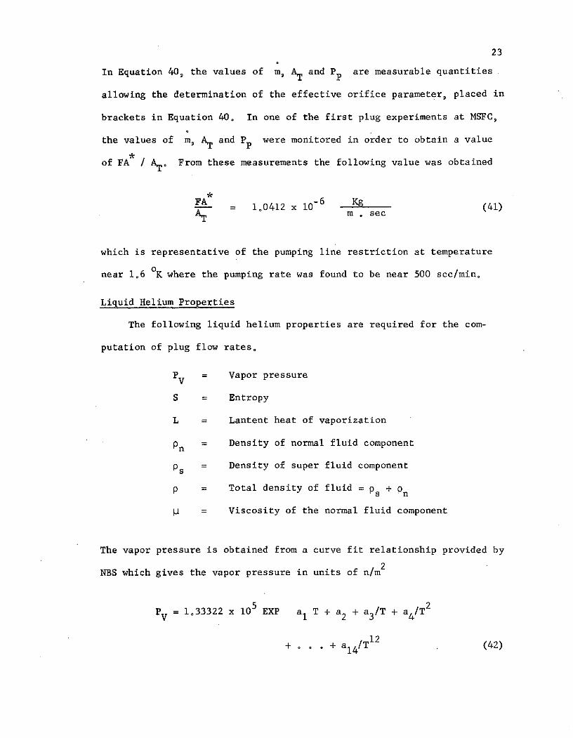
In Equation 40, the values of m, AT and Pp are measurable quantities

allowing the determination of the effective orifice parameter, placed in

brackets in Equation 40. In one of the first plug experiments at MSFC,

the values of m, AT and Pp were monitored in order to obtain a value

of FA / AT. From these measurements the following value was obtained

FA 1.0412 x 10- 6 Kg (41)AT m o sec

which is representative of the pumping line restriction at temperature

near 1.6 OK where the pumping rate was found to be near 500 scc/min.

Liquid Helium Properties

The following liquid helium properties are required for the com-

putation of plug flow rates.

PV = Vapor pressure

S = Entropy

L = Lantent heat of vaporization

pn = Density of normal fluid component

ps = Density of super fluid component

p = Total density of fluid = ps + pn

= Viscosity of the normal fluid component

The vapor pressure is obtained from a curve fit relationship provided by

NBS which gives the vapor pressure in units of n/m2

PV = 1.33322 x 105 EXP a T + a2 + a3/T + a 4/T2

+ . . + a14/T 1 2 (42)

24

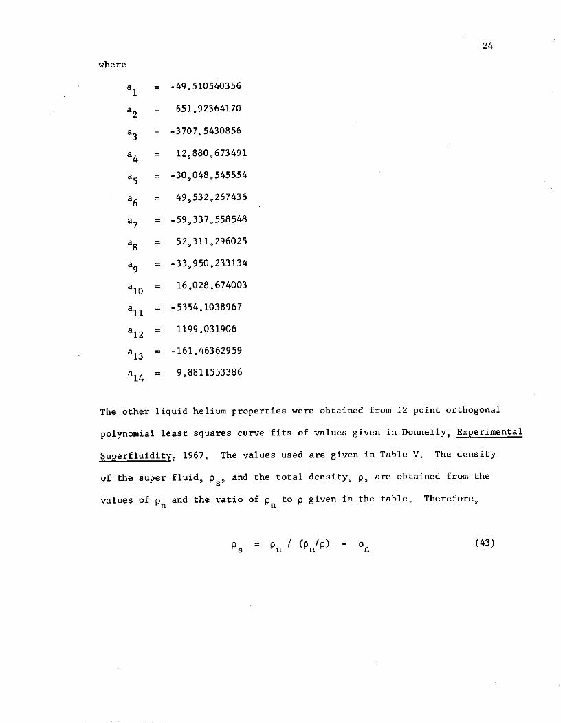
where

al = -49.510540356

a2 = 651.92364170

a3 = -3707.5430856

a4 = 12,880.673491

a5 = -30,048.545554

a6 = 49,532.267436

a7 = -59,337.558548

a8 = 52,311.296025

a9 = -33,950.233134

al0 = 16,028.674003

all = -5354.1038967

a1 2 = 1199.031906

a1 3 = -161.46362959

a1 4 = 9.8811553386

The other liquid helium properties were obtained from 12 point orthogonal

polynomial least squares curve fits of values given in Donnelly, Experimental

Superfluidity, 1967. The values used are given in Table V. The density

of the super fluid, ps, and the total density, p, are obtained from the

values of pn and the ratio of pn to p given in the table. Therefore,

Ps = on / (Pn/) - on (43)

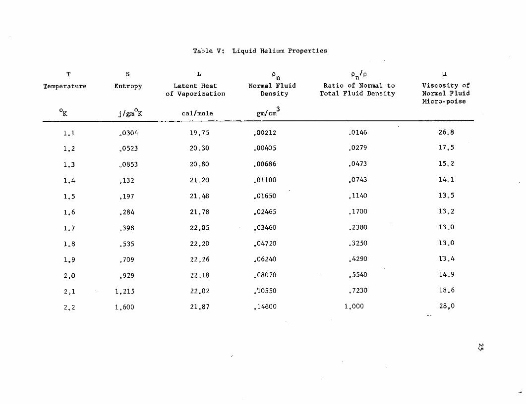
Table V: Liquid Helium Properties

T S L p pn/P

Temperature Entropy Latent Heat Normal Fluid Ratio of Normal to Viscosity ofof Vaporization Density Total Fluid Density Normal Fluid

Micro-poiseOK j/gmoK cal/mole gm/cm 3

1,1 .0304 19.75 .00212 .0146 26.8

1,2 .0523 20.30 .00405 .0279 17.5

1.3 .0853 20.80 .00686 .0473 15.2

1.4 .132 21.20 .01100 .0743 14.1

1.5 .197 21.48 .01650 .1140 13.5

1.6 .284 21.78 .02465 .1700 13.2

1.7 .398 22.05 .03460 .2380 13.0

1,8 .535 22.20 .04720 .3250 13.0

1,9 .709 22.26 .06240 .4290 13.4

2.0 .929 22.18 .08070 .5540 14.9

2,1 1,215 22.02 .10550 .7230 18.6

2.2 1,600 21.87 .14600 1.000 28,0

26

and

p = Ps + Pn (44)

Thermal Conductivity

Values of the thermal conductivity of the plug materials were ob-

tained from National Bureau of Standards, NBS Monograph 131, Thermal

Conductivity of Solids at Room Temperature and Below, 1973. At the

temperatures under consideration, the material thermal conductivities

are found to vary in a linear manner on a log-log plot of conductivity

and temperature. The thermal conductivity is then written as

Km = EXP (A + B log T) (45)

where A and B are the parameters of the straight line curve fit.

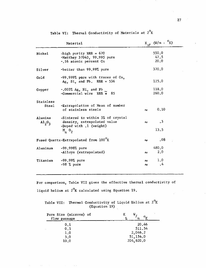
Thermal conductivity is found to be a strong function of the im-

purities or the alloy of the material under condideration. Table VI gives

a sampling of the thermal conductivities of various materials at 20K.

Figure 1 shows the variation of thermal conductivity with respect to

temperature for a number of materials.

Copper A12O3008 99S crystal

Copr

0 1-lytic)

iGermanium Figure 1:Brass(70-301

l- / Thermal conductivity variations of meels andStainless alloys (. . ), electrical insulators (---

steel l and a semi-conductor (Oo-o).

1/ Pyrex

SNylon

° 1

0.1 1.0 10 100 1000TEMPERATURE, K

27

Table VI: Thermal Conductivity of Materials at 20K

Material Km (W/m ° OK)

Nickel -high purity RRR = 670 550.0

-Matthey 37043, 99.995 pure 47.5-.16 atomic percent Cu 20.0

Silver -better than 99.99% pure 370.0

Gold -99.999% pdre with traces of Cu,

Ag, Si, and Pb. RRR = 536 125.0

Copper -.003% Ag, Ni, and Pb 118.0

-Commercial wire RRR 85 260.0

StainlessSteel -Extrapolation of Mean of number

of stainless steels 0.10

Alumina -Sintered to within 5% of crystal

Al203 density, estrapolated value .3-Doped with .1 (weight)M 02 13.5

Fused Quartz-Extrapolated from 1000K M .08

Aluminum -99.998% pure 480.0

-Alloys (extrapolated) 2.0

Titanium -99.99% pure M 1.0-98 % pure w .4

For comparison, Table VII gives the effective thermal conductivity of

liquid helium at 20K calculated using Equation 19.

Table VII: Thermal Conductivity of Liquid Helium at 20K(Equation 19)

Pore Size (microns) of K W/flow passage L m K

0.1 20.46

0.5 511.541.0 2,046.25.0 51,154.0

10.0 204,620.0

28

The thermal conductivity of the liquid is seen to be generally higher

than the material values given in Table VI except for pore sizes less

than .5 micron in diameter.

The thermal conductivities of the porous plug materials are ex-

pected to be less than the bulk material because of the granular structure

of the plug. Since thermal conductivity measurements were not made of

the porous materials used in the plug tests, the bulk properties are em-

ployed in the analysis with the realization that these conductivities

are likely higher than that of the porous material. The error made in

using the higher conductivity values is not important for large pore

plugs since the liquid helium thermal conductivity dominates the total

conductivity. For cases in which the conductivity of the plug material

is important (for pore sizes less than 0.5 micron), better values of

thermal conductivity are needed in order to accurately predict the plug

operation. While the relationships used here are expected to be in error

in absolute value, the variation with respect to temperature is repre-

sented. The characteristics of small-pore-size plugs revealed in ex-

periments may yield improved values of thermal conductivity when such

results are compared with those predicted.

In view of the lack of porous material conductivity information as

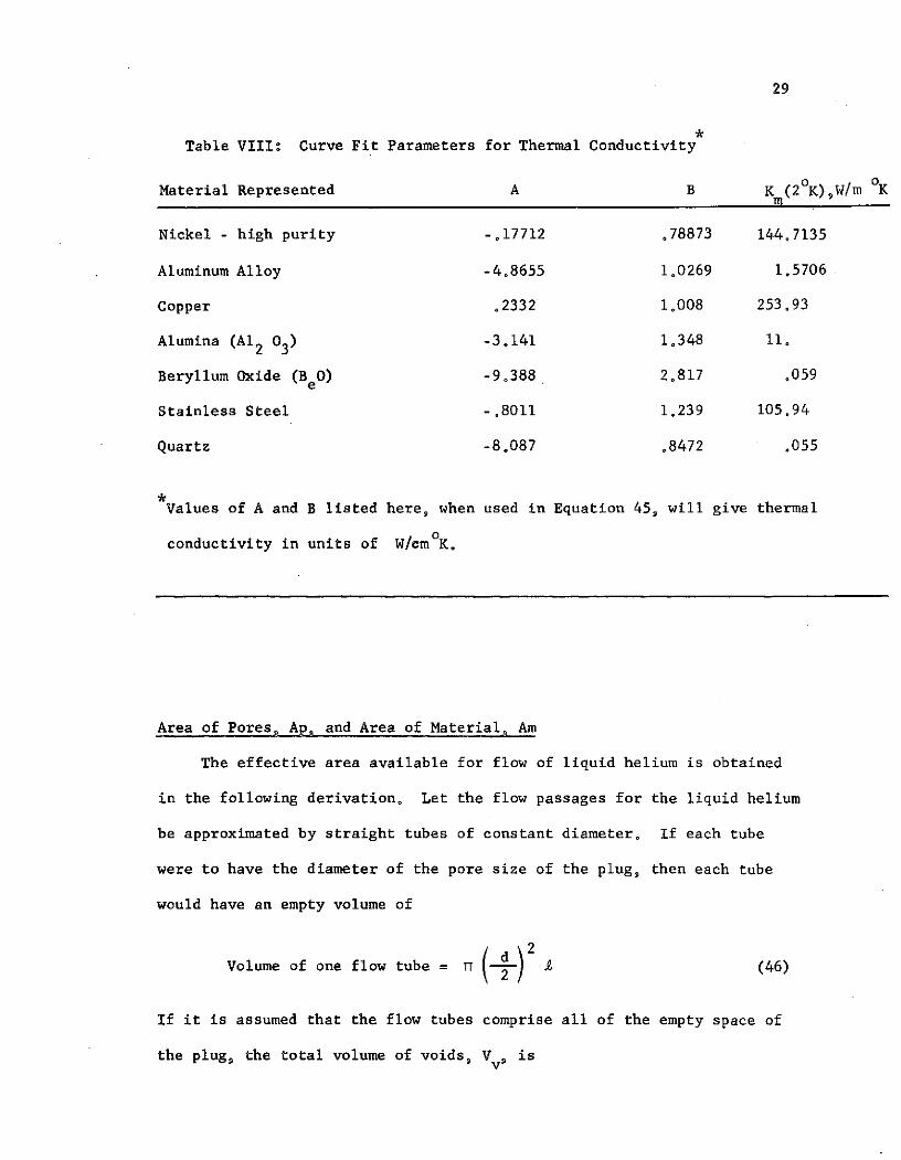
discussed above, curve fit parameters A and B were derived to represent

a number of different materials. These values are given in Table VIII.

29

Table VIII: Curve Fit Parameters for Thermal Conductivity

Material Represented A B K (20 K),W/m oK

Nickel - high purity -.17712 .78873 144.7135

Aluminum Alloy -4.8655 1.0269 1.5706

Copper .2332 1.008 253.93

Alumina (Al2 03) -3.141 1.348 11.

Beryllum Oxide (B 0) -9.388 2.817 .059

Stainless Steel -.8011 1.239 105.94

Quartz -8.087 .8472 .055

Values of A and B listed here, when used in Equation 459 will give thermal

conductivity in units of W/cmoK.

Area of Pores, Ap, and Area of Material, Am

The effective area available for flow of liquid helium is obtained

in the following derivation. Let the flow passages for the liquid helium

be approximated by straight tubes of constant diameter. If each tube

were to have the diameter of the pore size of the plug, then each tube

would have an empty volume of

Volume of one flow tube = ( 2 (46)

If it is assumed that the flow tubes comprise all of the empty space of

the plug, the total volume of voids, VvP is

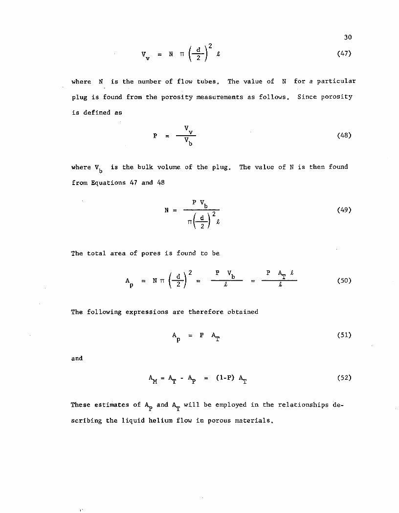
30

V = N ( d (47)v 2

where N is the number of flow tubes. The value of N for a particular

plug is found from the porosity measurements as follows. Since porosity

is defined as

VP V (48)

b

where Vb is the bulk volume of the plug. The value of N is then found

from Equations 47 and 48

PVN b (49)

2

The total area of pores is found to be

A N d 2 P Vb P AT (50)p 2)

The following expressions are therefore obtained

A = P AT (51)

and

AM = AT - A = ( 1 -P) AT (52)

These estimates of AP and AT will be employed in the relationships de-

scribing the liquid helium flow in porous materials.

31

Pore Size Estimation

The size of the pores in the porous plugs tested are not uniform as

evidenced by electron microscope pictures made of a number of the plugs.

The labeled values of pore size are very approximate and is meant as only

an estimate of the pore size, Since pore size is required in the eval-

uation of the equations presented here, it was decided to relate the

pore size to the measured value of permeability rather than use the

labeled value.

The permeability measurements given in Table III were least squares

fit with respect to the labeled pore size. A linear curve fit was em-

ployed with the result

d = ( F / P) / 2.5 (53)

where d is the pore diameter (assumed to have a circular cross section)

and A.F/A P corresponds to the room temperature helium gas flow given

in Table III in units of standard cubic centimeters per second per psi

of pressure drop (SCC/SEC/psi). The value of d determined using

Equation 46 will be given in units of microns.

Results

The above relationships were evaluated on the UAH Univac 1108 com-

puter. The computations were performed using the international system

of units. The flow rates were then converted to units of Standard Cubic

Centimeters per Minute (SCC/M) for ready comparison with the experimental

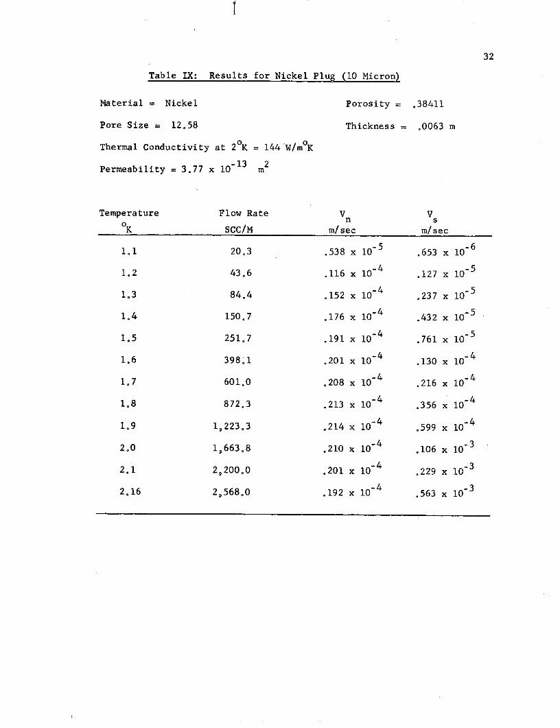
measurements which were made in those units. Table IX gives the results

for the first plug tested which was nickel having the properties listed

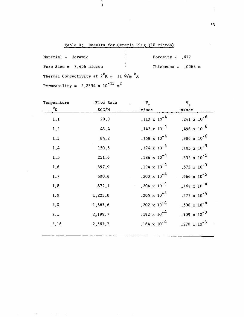
with the table. Table X gives results of the 10 micron ceramic and Table

XI gives results for .5 micron ceramic.

32

Table IX: Results for Nickel Plug (10 Micron)

Material = Nickel Porosity = .38411

Pore Size = 12.58 Thickness = .0063 m

Thermal Conductivity at 20K = 144 'W/mK

-13 2Permeability = 3.77 x 10 m

Temperature Flow Rate V Vn s

OK SCC/M m/sec m/sec

1.1 20.3 .538 x 10- 5 .653 x 10- 6

1.2 43.6 .116 x 10- 4 .127 x 10- 5

1.3 84.4 .152 x 10- 4 .237 x 10- 5

1.4 150.7 .176 x 10- 4 .432 x 10- 5

1.5 251.7 .191 x 10- 4 .761 x 10- 5

1.6 398.1 .201 x 10- 4 .130 x 10- 4

1.7 601.0 .208 x 10- 4 .216 x 10- 4

1.8 872.3 .213 x 10- 4 .356 x 10- 4

1.9 1,223.3 .214 x 10- 4 .599 x 10- 4

2.0 1,663.8 .210 x 10- 4 .106 x 10- 3

2.1 2,200.0 .201 x 10- 4 .229 x 10- 3

2.16 2,568.0 .192 x 10- 4 .563 x 10- 3

33

Table X: Results for Ceramic Plug (10 micron)

Material = Ceramic Porosity = .677

Pore Size = 7.456 micron Thickness = .0066 m

Thermal Conductivity at 20K = 11 W/m OK

-13 2Permeability = 2.2354 x 10 m

Temperature Flow Rate V Vn s

OK SCC/M m/sec m/sec

1,1 20.0 .113 x 10- 4 .241 x 10- 6

1.2 43.4 .142 x 10- 4 .496 x 10- 6

1.3 84.2 .158 x 10- 4 .986 x 10-6

1.4 150.5 .174 x 10- 4 .185 x 10- 5

1.5 251.6 .186 x 10- 4 .332 x 10- 5

1.6 397.9 .194 x 10- 4 .573 x 10- 5

1.7 600.8 .200 x 10- 4 .966 x 10- 5

1.8 872.1 .204 x 10- 4 ,162 x 10- 4

1.9 1,223.0 .205 x 10- 4 .277 x 10-4

2.0 1,663.6 .202 x 10- 4 .500 x 10- 4

2.1 29199.7 .192 x 10- 4 .109 x 10-3

2.16 2,567,7 .184 x 10- 4 .270 x 10- 3

34

Table XI: Results for Ce amic Plug (.5 micron)

Material = Ceramic Porosity = .548

Pore Size = .1792 micron Thickness = .0065 m

Thermal Conductivity at 2K = 11 W/m OK-15 2Permeability 5.3726 x 10 m

Temperature Flow Rate V Vn sOK SCC/M m/sec m/sec

-5 -1.1 16.0 .260 x 10-5 .366 x 10-6

1.2 30.7 .117 x 10-4 .455 x 10-6

1.3 52.2 .336 x 10-3 -.304 x 10-6

-4 -1,4 83.9 .747 x 10 -.377 x 10-5

-3 -1.5 130.9 .141 x 10-3 -.146 x 10-

1,6 204.5 .231 x 10-3 -.409 x 10-4

1.7 321.7 .338 x 10-3 -. 954 x 10- 4

1,8 502.7 .448 x 10-3 -.197 x 10-3

-331,9 761.3 .543 x 10-3 -. 374 x 10- 3

-332.0 1,096.1 .600 x 10-3 -.685 x 10-3

2.1 1,484.9 .606 x 10-3 -.145 x 10- 2

2.16 1,717.4 .580 x 10- 3 -. 351 x 10 - 2

35

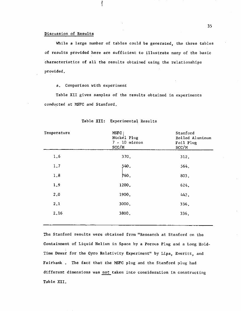
Discussion of Results

While a large number of tables could be generated, the three tables

of results provided here are sufficient to illustrate many of the basic

characteristics of all the results obtained using the relationships

provided.

a. Comparison with experiment

Table XII gives samples of the results obtained in experiments

conducted at MSFC and Stanford.

Table XII: Experimental Results

Temperature MSFC I StanfordNickel Plug Rolled Aluminum7 - 10 micron Foil PlugSCC/M SCC/M

1.6 370. 312.

1.7 40o 564.

1.8 60. 803°

1.9 1200. 624.

2,0 1900. 442.

2,1 3000. 336.

2,16 3800. 336.

The Stanford results were obtained from "Research at Stanford on the

Containment of Liquid Helium in Space by a Porous Plug and a Long Hold-

Time Dewar for the Gyro Relativity Experiment" by Lipa, Everitt, and

Fairbank . The fact that the MSFC plug and the Stanford plug had

different dimensions was not taken into consideration in constructing

Table XII.

36

The experimental results given in Table XII show similar total flow

rates in the range of 1.6 OK to 1.8 OK for both the MSFC and Stanford

plugs. However, at 1.8 OK and higher, the Stanford plug shows a reduction

in flow rate with increasing temperature to the lambda point. The MSFC

plug on the other hand shows a monatomically increasing flow rate with

increasing temperature which is in agreement with that predicted by the

equations developed here as given in Tables IX, X, and XI.

The theory developed here is found to predict the behavior of the

MSFC large pore Nickel plug with respect to temperature. While the

shape of the flow rate versus temperature curve is accurately predicted,

the values predicted are about 30%,less than that measured at temperatures

near the lambda point. The agreement at lower temperatures is progressively

better until the best agreement is reached at 1.6 K. (7.5% error).

The reason the theory has such large error at the higher temperatures

FA*was traced to the value of the pumping factor A used in the program.

This factor was determined for flow measurements made near 1.6 OK. If

the pumping line restriction were an ideal choked orifice as modeled,

this factor would be constant. H ever, since the restriction is more

complex, the factor is not constat and is found to increase as the

pressure on the gas side of the plug increases. Future work will modify

the model of the pumping line restriction to yield improved comparison

with experiment.

OF Polimi I~' ~RUA=~e

FINANCIAL STAUJS REPORT

Contract No. NAS8-29316

f. Expnditures to date as of June 30, 1974 beginning with the UAH

fisca yarw October T, 1973 and each previous year, if any. $102,326.54

I. Forecast of funds required for compltion: 61,914.46

II. Proble areas:

SORIoR PAGEOF POOR QUAIXY