NBER WORKING PAPER SERIES

RENT-SHARING, HOLDUP, AND WAGES:EVIDENCE FROM MATCHED PANEL DATA

David CardFrancesco Devicienti

Agata Maida

Working Paper 16192http://www.nber.org/papers/w16192

NATIONAL BUREAU OF ECONOMIC RESEARCH1050 Massachusetts Avenue

Cambridge, MA 02138July 2010

We thank Raj Chetty, Carlo Gianelle, Peter Kuhn, Alex Lefter, Bentley MacLeod, Enrico Moretti,Luigi Pistaferri, Ben Sand, and seminar participants at the LABORatorio Revelli, Berkeley IRLE,and the Federal Reserve Board of San Francisco for comments and suggestions. We are especiallygrateful to Giuseppe Tattara for providing the Veneto Work History Data, and to Carlo Gianelle andMarco Valentini for assistance in using these data. Agata Maida is pleased to acknowledge supportfrom the Leibniz Association though the Labor Market Institutions project at RWI-Essen. The viewsexpressed herein are those of the authors and do not necessarily reflect the views of the National Bureauof Economic Research.

NBER working papers are circulated for discussion and comment purposes. They have not been peer-reviewed or been subject to the review by the NBER Board of Directors that accompanies officialNBER publications.

© 2010 by David Card, Francesco Devicienti, and Agata Maida. All rights reserved. Short sectionsof text, not to exceed two paragraphs, may be quoted without explicit permission provided that fullcredit, including © notice, is given to the source.

Rent-sharing, Holdup, and Wages: Evidence from Matched Panel DataDavid Card, Francesco Devicienti, and Agata MaidaNBER Working Paper No. 16192July 2010JEL No. J31

ABSTRACT

When wage contracts are relatively short-lived, rent sharing may reduce the incentives for investmentsince some of the returns to sunk capital are captured by workers. In this paper we use a matched worker-firmdata set from the Veneto region of Italy that combines Social Security earnings records for employeeswith detailed financial information for employers to measure the degree of rent sharing and test forholdup. We estimate wage models with job match effects, allowing us to control for any permanentdifferences in productivity across workers, firms, and job matches. We also compare OLS and instrumentalvariables specifications that use sales of firms in other regions of the country to instrument value-addedper worker. We find strong evidence of rent-sharing, with a “Lester range” of variation in wages betweenprofitable and unprofitable firms of around 10%. On the other hand we find little evidence that bargaininglowers the return to investment. Instead, firm-level bargaining in Veneto appears to split the rentsafter deducting the full cost of capital. Our findings are consistent with a dynamic bargaining model(Crawford, 1988) in which workers pay up front for the returns to sunk capital they will capture inlater periods.

David CardDepartment of Economics549 Evans Hall, #3880University of California, BerkeleyBerkeley, CA 94720-3880and NBERcard@econ.berkeley.edu

Francesco DevicientiUniversity of Torino Faculty of EconomicsCorso Unione Sovietica 218bis10134 TorinoITALYfdevic@tiscali.it

Agata MaidaRWI-EssenHohenzollernstr. 1-3Essen 45128GERMANYagata.maida@laboratoriorevelli.it

1

A long-running strand of research has argued that employees share some of the rents

earned by their employers.1 Early studies used data on wages and profitability at the industry

level (e.g., Slichter, 1950; de Menil, 1971; Dickens and Katz, 1986) while later studies use firm-

level data (e.g., Nickell and Wadhwani, 1990; Chistofides and Oswald, 1992; Abowd and

Lemieux, 1993; Blanchflower, Oswald and Sanfey, 1996; Hildreth and Oswald, 1997; Arai,

2003). Both literatures show a positive correlation between profitability and wages. How much

of this is due to the sorting of high-ability workers to high-profit industries or firms is still

unclear. Recent studies that use matched worker/firm data to control for unobserved ability find

smaller but generally significant effects of profitability on wages (e.g., Margolis and Salvanes,

2001; Martins, 2009; Guertzgen, forthcoming).2

In a dynamic setting it is well known that bargaining over rents can lead to a “holdup”

problem (Baldwin, 1983; Grout, 1984; Che and Sakovics, 2008; MacLeod, 2010). Specifically,

when capital is sunk, bargaining over quasi-rents can divert some of the return on investment to

workers, potentially causing firms to under-invest.3 Building on this insight, Connolly et al.

1The idea of rent-sharing by a cartel of workers appears in Adam Smith (1976, Book I, Chapter 8). The post-war neo-institutionalists (e.g., Lester, 1952, Slichter, 1950) emphasized firm profitability (or ability to pay) as an important determinant of wages. De Menil (1971) laid out the basic model of bargaining that we use in this paper and has been adopted by many subsequent authors (e.g., Svejnar, 1986; Abowd and Lemieux, 1993; Blanchflower, Oswald and Sanfey, 1996).

2Guiso, Pistaferri, and Schivardi (2005) study the effect of firm-specific productivity shocks on employee wages using a matched longitudinal data set similar to ours. Although their empirical analysis focuses on risk sharing, rather than rent-sharing, their results suggest that firm-level productivity shocks have a positive effect on wages.

3The problem was recognized by Simons (1944) who wrote: “Frankly, I can see no reason why strongly organized workers, in an industry where huge investment is already sunk in highly durable assets, should ever permit a return on investment sufficient to attract new capital.”

2

(1986), Denny and Nickell (1992), and Bronars and Deere (1993) have argued that unionized

firms invest less than their non-union competitors, contributing to the decline in union coverage

in many countries (see also Addison and Hirsch, 1989, and Hirsch, 2004).4

In this paper we use a matched data set that combines administrative earnings records for

individual employees with detailed balance sheet data for their employers to measure the degree

of rent sharing by firms in the Veneto region of Italy. We implement a simple test for the

presence of holdup based on the fraction of capital costs that are deducted from the quasi-rent

expression in the wage determination model. When capital costs are fully deducted firms have

the right incentives to invest. When some of the returns to previous investments are included as

quasi-rent, however, firms that invest more will pay higher wages in the future, generating a

holdup problem.

Our estimation sample includes about 400,000 workers and 7,000 firms, with wages and

detailed financial information covering the period from 1995 to 2001. These data enable us to

estimate wage models that include job match effects (i.e., dummies for each worker-firm pair

observed in the sample), as well as time-varying worker and firm variables. Match effects

control for any permanent differences between workers, firms, and job-matches. For about

three-quarters of the sample we can also identify the minimum wage specified by the sector-wide

contract that covers the employment relationship.5 Thus, we can measure the wage premium that

4As shown by Crawford (1988) holdup does not necessarily arise in long term relationships governed by short term contracts. It should also be noted that not all previous studies have found that unionized firms have lower investment rates – see e.g., Machin and Wadhwani (1991).

5In Italy contracts negotiated at the sector-level between national unions and employer groups are extended to cover essentially all employees. The sectoral contracts specify minimum wages by industry and occupation category (typically 5 or more categories).

3

arises through a combination of firm-level contracting and individual bargaining.6 In an

institutional setting like Italy with binding sectoral contracts, this premium is arguably the

appropriate earnings concept for measuring firm-specific rent-sharing.7

We relate individual earnings to a firm-specific quasi-rent measure, defined as value

added per worker net of the opportunity cost of labor and some share of the cost of capital per

worker. A longstanding concern in the rent-sharing literature is the potential endogeneity of

profitability, arising through efficiency wage effects or other channels.8 A related problem is

measurement error in value added, which is likely to be exacerbated by a within-spell estimation

strategy. To address both issues we use the revenues of firms in the same narrowly defined

sector in other regions of Italy to construct an instrumental variable for value-added per worker

for employers in Veneto. Our identifying assumption is that industry demand shocks affect firm-

level profitability but have no direct effect on local labor supply.

Our empirical findings point to two main conclusions. First, consistent with existing

studies, we find that more profitable employers pay higher wages. In simple cross-sectional

models the estimated elasticity of wages with respect to quasi-rents per worker is on the order of

6-8%. Within-job-spell estimates obtained by OLS are substantially smaller, but appear to be

attenuated by measurement errors and transitory fluctuations in value-added. When we

6During our sample period about 40% of workers were covered by firm-level contracts that set pay scales above the sectoral minimum.

7Cristini and Leoni (2007) specify a two-level bargaining model that describes the determination of the sector wide minimum wages and the firm-specific wage premium. We abstract from the first and concentrate on the second.

8See e.g., Abowd and Lemieux (1993) and Van Reenen (1996). These authors are most concerned about the possibility that more profitable firms hire high-ability workers. As noted, by including job match dummies we control for any permanent differences in ability between employees (including differences that are rewarded more highly in some firms than others).

4

instrument value-added using data for firms in the same sector in other regions we obtain

estimates of the rent sharing elasticity in the range of 3-4% – roughly one-half as large as the

cross-sectional estimates. Second, our estimates suggest that firm-level bargaining in Italy is

driven by a quasi-rent measure that deducts the full cost of capital. Though we cannot rule out a

small degree of holdup, the point estimates from a range of specifications are consistent with an

implicit user cost of capital of around 10% – close to the benchmark suggested by several recent

studies (Arachi and Biagi, 2005; Elston and Rondi, 2006).

Full offset of capital costs is consistent with a dynamic bargaining model in which

workers pay up-front for the portion of returns to sunk investments they will capture in future

bargaining (Crawford, 1988). In such a model the appropriate expression for the quasi-rent

contains a deduction for the cost of the non-irreversible share of the current capital stock, plus a

deduction for future holdup of the irreversible share of future capital. When the firm’s capital

stock is growing at the real interest rate the sum of these deductions equals the full cost of

capital.

II. A Model of Rent Sharing and Wage Determination

In this section we outline a simple dynamic model of wage bargaining between a firm

and a collection of identical workers. We assume that wages are renegotiated every period, and

that some fraction of the current capital stock is sunk, and cannot be resold by the firm during the

current period.9 Although this is a textbook setting for holdup (e.g., Cahuc and Zylberberg, 2004,

pp. 543-545) we show that the holdup problem is mitigated when bargaining today anticipates

9Thus, we are modeling a long term relationship governed by incomplete short term contracts. Our model is an adaptation of the one presented in Crawford (1988).

5

rent-sharing tomorrow. Instead, as in Becker’s (1962) on-the-job training model, workers make

an up-front contribution by accepting lower wages today in return for a share of future quasi-

rents. When workers and firms share the same discount rate and workers’ bargaining power is

constant over time this restores the incentive for firms to invest efficiently.

a. Basic Model with Fixed Employment

We start with the case where employment is fixed at L. We adopt a two-period model and

assume that the firm’s revenue in period t (net of raw materials costs) is R(Kt, θt) where θt is a

fully anticipated demand shock and Kt is the firm’s capital stock, assumed to be determined one

period in advance. The firm’s profit in period t is:

R(Kt, θt) ! wtL ! rt Kt ,

where wt represents the negotiated wage and rt represents the user cost of capital. We assume

that workers’ preferences over wage outcomes in period t are represented by the excess wage

bill:

u(wt, L) = (wt!mt)L ,

where mt represents in the opportunity cost of labor.10 Finally, we assume that the parties

discount the future at a common discount rate β.

In the second period the only decision variable is the wage, w2. Following de Menil

(1971) and subsequent authors we assume that w2 is determined by generalized Nash bargaining:

(1) w2 = argmax [ u(w, L) ! u02 ]γ [ π(w, r2; K2, L, θ2) ! π0

2 ]1!γ , w 10In our empirical work we assume that mt is either the minimum sectoral wage, or the average wage in the sector. The assumption of an excess wage bill objective means that in a setting with variable employment, the surplus-maximizing choice of employment equates the marginal product of labor to the outside wage mt.

6

where u0

2 and π02 represent the fallback positions of the parties if no agreement is reached, and γ

represents the relative bargaining power of workers. On the workers’ side we assume that u02 =

0. On the firm’s side we assume that a fraction δ of the capital stock can be resold for other uses

in the event of no agreement.11 In this case, the fallback position of the firm is a net cash flow of

!(1!δ)r2K2. Combining these assumptions with equation (1), the second period wage

maximizes:

(2) [ (w2 !m2)L ]γ [ R(K2, θ2) ! w2L ! δr2K2 ]1!γ . The associated first order condition for w2 can be re-arranged as:

(3) w2 = m2 + γ Q2/L ,

where

Q2 / R(K2, θ2) ! m2 L ! δ r2K2

is the “quasi-rent” associated with reaching agreement in period 2. Notice that when δ=1,

investment is reversible and the appropriate quasi-rent is value-added minus the opportunity cost

of labor minus the full cost of capital. On the other hand, when δ=0, all investment is sunk and

the appropriate quasi-rent is value-added minus the opportunity cost of labor.

The second period profits of the firm are:

(4) π2 = (1!γ)Q2 ! (1!δ)r2K2 ,

= (1!γ) [ R(K2, θ2) ! m2 L ] ! r2(1!γδ)K2 .

Differentiating the second line with respect to K2 yields:

(5) Mπ2/MK2 = (1!γ) [ MR/MK2 ! r2(1!γδ)/(1!γ) ] .

If the firm chooses K2 to maximize second period profits, this first order condition implies that it

11A similar assumption is made by Grout (1984) who distinguishes between the price

7

will under invest whenever δ<1. In particular, when a fraction 1!δ of investment is sunk, the

firm acts as if the user cost of capital is r2(1!γδ)/(1!γ) > r2. For this reason a number of

previous authors have concluded that short term bargaining with sunk investment imposes a

“tax” on capital.12

The intuition underlying equation (5) is potentially misleading, however, because it fails

to recognize that the outcome of bargaining in period 1 will in general depend on the expected

outcomes of bargaining in period 2.13 Assume that the parties bargain in period 1 anticipating the

returns in period 2 implied by the wage bargain of equation (3) (i.e., net utility of (w2!m2)L =

γQ2 and profits specified in equation (4)). As in period 2, assume that the fallback position of

workers in the event of no agreement in period 1 is a payoff of 0 (for one period), while the

fallback for the firm is a cash flow of !r1(1!δ)K1. In this case, bargaining in period 1 will

maximize the expression

(6) [ (w1!m1)L + βγQ2 ]γ [ R(K1,θ1)!w1L!δr1K1 + β( (1!γ)Q2 ! r2(1!δ)K2 )) ]1!γ.

As was emphasized in the efficient contracting literature (e.g., MacDonald and Solow, 1981;

Brown and Ashenfelter, 1986) it is potentially important to consider whether w1 and K2 are

jointly determined in period 1, or whether the firm selects K2 unilaterally before w1 is

determined. For the moment, consider the case where K2 is jointly determined. Then it is easily

shown that maximization of (6) requires MR(K2, θ2)/MK2 = r2, i.e., an “efficient” level of

paid for capital and its resale value.

12For example, Cahuc and Zylberberg (2004, pp. 543-545) present a simple analysis of the sunk investment case that yields essentially the same formula as equation (5) with δ=0.

13The same point was made by Becker (1962) in an analysis of the return to general human capital investments.

8

investment.14

Turning to the wage, the first order condition for w1 can be written as:

(7) w1 ! m1 = γQ1/L, where

Q1 / R(K1,θ1) ! m1L ! δr1K1 ! β(1!δ)r2K2 .

Note that when the bargaining relationship is expected to continue the effective quasi-rent in

period 1 deducts a fraction δ of current capital costs, and a complementary fraction 1!δ of future

costs (discounted by β). In essence, the firm is compensated ex ante for the share of returns to

capital it will lose due to rent sharing in the second period. Note that if the return to capital is

constant (r1=r2=r) and the capital stock is growing at the “steady state” rate 1/β then K2=K1/β and

the quasi-rent expression becomes:

(8) Q1 = R(K1 , θ1) ! m1L ! rK1 .

In this case the appropriate expression for the quasi-rent deducts the full cost of capital even

though capital is sunk.

Importantly, the expression for w1 in equation (7) remains the same whether K2 is

determined jointly by the parties, or whether the firm chooses K2 unilaterally, prior to wage

bargaining in period 1. In the latter case equations (4) and (7) can be combined to show that:

(9) π1 + βπ2 = (1!γ) [ R(K1,θ1) ! m1L ! δr1K1 ] ! γ(1!δ)r1K1

+ β(1!γ) [ R(K2,θ2) ! m2L ! r2K2 ] .

An immediate implication is that

14For a maximand of the form [ a + bw + g(K) ]γ [ c ! bw + h(K) ]1!γ , if w and K are the choice variables and there are no constraints on w the first order conditions require that gN(K)+hN(K)=0. In this setup w is an efficient transfer and any bargaining solution requires a surplus-maximizing choice of K. In applying this observation to (6) note that the sum of the second period payoffs to workers and the firm is equal to R(K2, L, θ2)!m2L!r2K2.

9

M[π1 + βπ2]/MK2 = β(1!γ) [ MR(K2,θ2)/MK2 ! r2 ] .

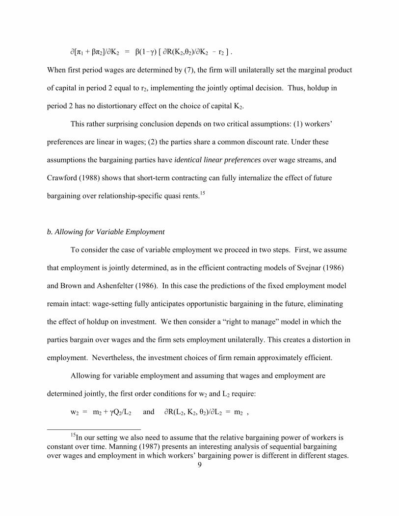
When first period wages are determined by (7), the firm will unilaterally set the marginal product

of capital in period 2 equal to r2, implementing the jointly optimal decision. Thus, holdup in

period 2 has no distortionary effect on the choice of capital K2.

This rather surprising conclusion depends on two critical assumptions: (1) workers’

preferences are linear in wages; (2) the parties share a common discount rate. Under these

assumptions the bargaining parties have identical linear preferences over wage streams, and

Crawford (1988) shows that short-term contracting can fully internalize the effect of future

bargaining over relationship-specific quasi rents.15

b. Allowing for Variable Employment

To consider the case of variable employment we proceed in two steps. First, we assume

that employment is jointly determined, as in the efficient contracting models of Svejnar (1986)

and Brown and Ashenfelter (1986). In this case the predictions of the fixed employment model

remain intact: wage-setting fully anticipates opportunistic bargaining in the future, eliminating

the effect of holdup on investment. We then consider a “right to manage” model in which the

parties bargain over wages and the firm sets employment unilaterally. This creates a distortion in

employment. Nevertheless, the investment choices of firm remain approximately efficient.

Allowing for variable employment and assuming that wages and employment are

determined jointly, the first order conditions for w2 and L2 require:

w2 = m2 + γQ2/L2 and MR(L2, K2, θ2)/ML2 = m2 ,

15In our setting we also need to assume that the relative bargaining power of workers is constant over time. Manning (1987) presents an interesting analysis of sequential bargaining over wages and employment in which workers’ bargaining power is different in different stages.

10

where

Q2 = R(L2, K2, θ2) ! m2 L2 ! δ r2K2 .

Likewise, the first order conditions for the optimal choices of w1 and L1 require

w1 = m1 + γQ1/L1 and MR(L1, K1, θ1)/ML1 = m1 ,

where

Q1 = R(L1, K1, θ1) ! m1L1 ! δ r1K1 ! β(1!δ)r2K2.

Finally, the optimal choice for K2 (which we assume is also made in period 1) requires

r2 = MR(L2, K2, θ2)/MK2 .

The expressions for w1 and w2 are the same as in the fixed employment case, except that L is

replaced by the efficient level of employment that equates the marginal product of labor with the

outside wage mt. The expression for the firm’s discounted profits also remains the same as in

equation (9) (with the appropriate substitution for Lt), implying that the firm unilaterally selects

the jointly optimal investment choice when wages and employment are jointly determined in a

sequence of short-term bargains. Consequently, with jointly determined employment, holdup

does not distort investment.

When the firm sets employment unilaterally the analysis is more complicated because

now wages have three competing functions: to split the surplus between the parties; to regulate

incentives for investment; and to allocate labor within the period. The conflict between these

objectives causes some inefficiency. In particular, with unilateral employment setting any

bargained wage above the alternative wage implies that employment is set below the efficient

choice that maximizes the joint surplus of the parties. To first order, however, this distortion

does not spill over to investment: as in the fixed employment case the negotiated wage contains a

11

discount for future holdup, and the level of capital selected by the firm sets the marginal product

of capital approximately equal to the interest rate.

Specifically, in Appendix A we show that when: (i) the firm sets employment taking the

wage as given; (ii) wage bargaining maximizes a generalized Nash objective with a fixed weight

γ for workers; and (iii) the negotiated mark-up over the alternative wage is approximately

constant over time; the first-period wage is approximately

(10) w1 = m1 + γ Q1*/L1

* , where

Q1* = R(L1

*, K1, θ1) ! m1 L1* ! δ r1 K1 ! β(1!δ) r2 K2

* and L1

* = L1(mt , K1, θ1)

are the “efficient” levels of quasi-rent and employment, respectively, K1 is the initial capital

stock (inherited from the past), and K2* is the “efficient” capital stock in period 2 (defined

precisely in the Appendix).16 Moreover, as in the simple case with fixed employment, the firm

selects the efficient capital stock K2*.

These results imply that when the firm sets investment and employment unilaterally, w1

and K2 will be set at (approximately) the same levels as would occur under joint employment

setting. However, the firm’s employment choice L1 will be below the efficient level, L1*, and the

observed measure of rents in period 1 will differ from the measure Q1* that determines wages. In

particular, we show in Appendix A that the observed measure of rents in period 1 is:

(11) Q1 = R(L1, K1, θ1) ! m1 L1 ! δ r1 K1 ! β(1!δ) r2 K2

16The derivation of these expressions uses a linearization of the firm’s profit functions in each period around the profit associated with the outside wage (m1 or m2). Assuming that γ is on the order of 10-20% and the ratio of profits to the wage bill is in the range of 0 to 1, the percentage wage markup implied by (10) is under 20% and the assumption of local linearity is reasonable. The average markup of wages over the sectoral minimum in our sample ranges from 23% to 26%, so we believe condition (iii) is reasonable.

12

. Q1* (1 + εγg1

* )

where ε #0 is the elasticity of the firm’s labor demand schedule and g1* / (w1!m1)/m1 is the

negotiated markup of the contract wage over the outside wage. Approximating L1 =

L1*(1+εg1

*), the “efficient” quasi-rent per worker is

(12) Q1*/L1

* = λ Q1/L1 , where

λ . (1 + εg1*(1!γ) ) # 1 .

Thus, observed quasi-rent per worker overstates the appropriate expression Q1*/L1

* in the wage

determination model. For example, assuming a demand elasticity of ε=!1, a rent-share

parameter of γ=0.20, and a markup of g1*=0.15, the implied value of λ is approximately 0.9.

c. Empirical Implementation

In the derivation of equation (10) we assumed that capital is homogeneous and that a

fraction δ of the capital stock in each period can be put to other uses during a dispute, leading to

a quasi-rent measure of the form:

Qt* = R(Lt

*, Kt, θt) ! mt Lt* ! δ rt Kt ! β(1!δ) rt+1 Kt+1 .

Since capital adjusts irregularly and is measured with some error, it is difficult to separately

identify the effects of Kt and Kt+1 on wages in any period.17 Moreover we do not have period-

specific estimates of the cost of capital. In view of these limitations we make the assumptions

that rt = rt+1 = r, and that the rate of growth of capital is close to the discount rate (i.e., Kt+1 =

(1/β)Kt). In this case, our bargaining model predicts that the appropriate quasi-rent measure for

wage determination in period t is:

17Note however that prior to a large new investment workers are predicted to take a wage cut in anticipation of higher rents in the future. Such dynamic behavior is arguably the strongest

13

Qt* = R(Lt

*, Kt, θt) ! mt Lt* ! r Kt .

Substituting this expression into equation (10) yields:

wt = mt + γ [ R(Lt*, Kt, θt) ! mt Lt

* ! r Kt ] / Lt* ,

and using (12) we obtain a relationship between wages and observed quasi-rents:

(13) wt = mt + λγ [ R(Lt, Kt, θt) ! mt Lt ! r Kt ] / Lt

= mt (1 ! λγ) + λγ R(Lt, Kt, θt)/Lt ! λγr (Kt/Lt) .

Inspection of equation (13) points to two immediate predictions: (1) value-added per

worker affects wages with a coefficient λγ that understates the true rent-splitting parameter γ to

the extent that λ < 1; (2) controlling for value-added per worker, capital per worker affects wages

with a coefficient of !λγr. In contrast, in the presence of distortionary holdup, we would expect

the coefficient of capital per worker to be smaller than !λγr (in absolute value). In the extreme

case of complete holdup the predicted coefficient of capital per worker is 0. Thus, our main

empirical focus is on comparing the estimated effects of value-added per worker and capital per

worker on negotiated wages, and testing whether the ratio is consistent with existing estimates of

the cost of capital. We also compare the effects of different types of capital (e.g., physical

versus working capital) and distinguish between firms with higher and lower levels of debt to

check whether there is a larger offset for investments that are financed by debt (as suggested by

Dasgupta and Sengupta, 1993).

The literature on capital investment in Italy suggests that during the mid-to-late 1990s a

reasonable estimate of the user cost of capital is in the range of 8-12%. Elston and Rondi (2006)

report a distribution of estimates of the user cost of capital for publicly traded Italian firms in the

implication of our model. We thank Peter Kuhn for pointing this out.

14

1995-2002 period, with a median of 11% (Elston and Rondi, 2006, Table A4). Arachi and Biagi

(2005) calculate the user cost of capital, with special attention to the tax treatment of investment,

for a panel of larger firms over the 1982-1998 period. Their estimates for 1995-1998 are in the

range of 10-15% with a value of 11% in 1998 (Arachi and Biagi, 2005, Figure 2).18

In our estimation we adopt a log-linearization of equation (13). Specifically, building on

the observation that wages are approximately log-normally distributed, and that standard

covariates like gender, age, and job tenure exert a proportional effect on wages, we fit models of

the form:

(13N) log(wit) = log(ait) b1 + Xitb2 + VAj(i,t),t b3 + KLj(i,t),t b4 + ξit ,

where wit is the average daily wage earned by worker i in year t, ait is a (potentially noisy)

measure of the opportunity wage for the worker in that year, Xit represents a vector of measured

characteristics of the worker, VAj(i,t),t represents measured value-added per worker at the firm

j(i,t) that employed worker i in period t, KLj(i,t),t is measured capital per worker at the firm, and

ξit is an error term. The prediction of no distortionary holdup implies that b4 =! r b3, while full

holdup implies b4 = 0. We fit this model using a variety of estimation strategies, including OLS,

OLS with firm-worker-match fixed effects, and instrumental variables (IV) with match fixed

effects, treating value added per worker (and in some cases capital per worker) as endogenous.

18Franzosi (2008) calculates the marginal user cost of capital taking into account the differential costs of debt and equity financing, and the effects of tax reforms in 1996 and 1997. Her calculations suggest that the marginal user cost of capital was about 7.5% pre-1996 for a firm with 60% debt financing, and fell to 6% after 1997.

15

III. Institutional Background, Data Sources, and Descriptive Overview

a. Institutional Background

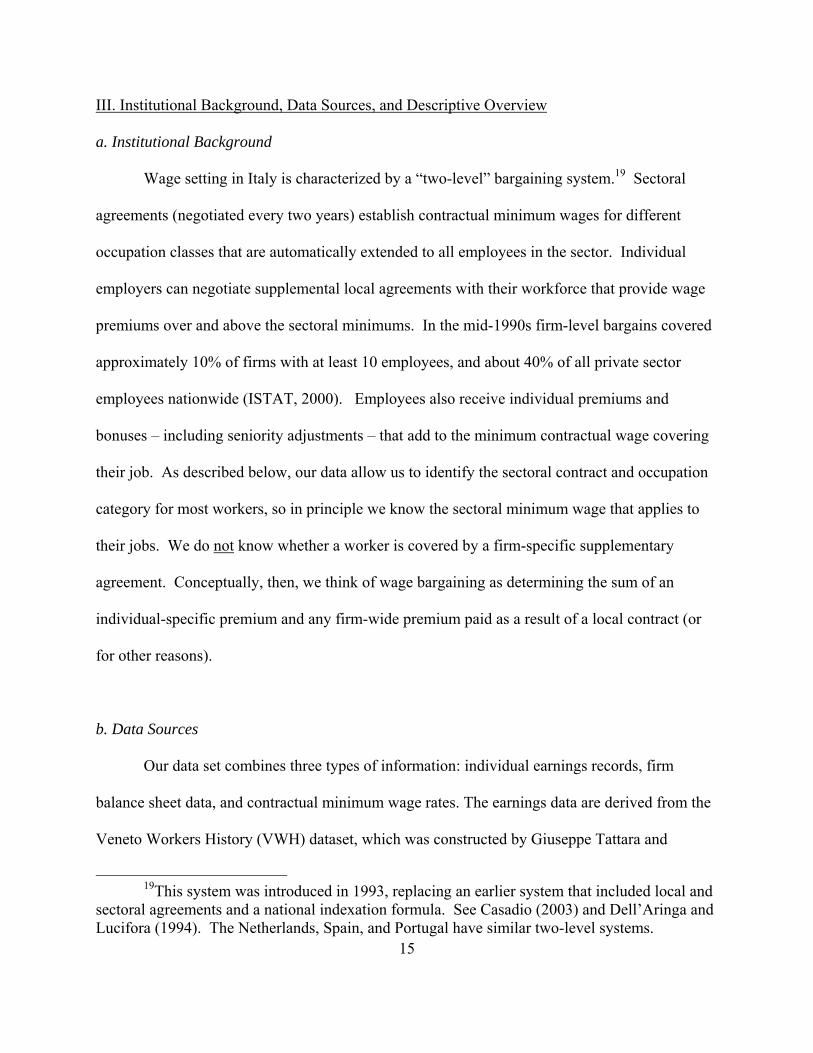
Wage setting in Italy is characterized by a “two-level” bargaining system.19 Sectoral

agreements (negotiated every two years) establish contractual minimum wages for different

occupation classes that are automatically extended to all employees in the sector. Individual

employers can negotiate supplemental local agreements with their workforce that provide wage

premiums over and above the sectoral minimums. In the mid-1990s firm-level bargains covered

approximately 10% of firms with at least 10 employees, and about 40% of all private sector

employees nationwide (ISTAT, 2000). Employees also receive individual premiums and

bonuses – including seniority adjustments – that add to the minimum contractual wage covering

their job. As described below, our data allow us to identify the sectoral contract and occupation

category for most workers, so in principle we know the sectoral minimum wage that applies to

their jobs. We do not know whether a worker is covered by a firm-specific supplementary

agreement. Conceptually, then, we think of wage bargaining as determining the sum of an

individual-specific premium and any firm-wide premium paid as a result of a local contract (or

for other reasons).

b. Data Sources

Our data set combines three types of information: individual earnings records, firm

balance sheet data, and contractual minimum wage rates. The earnings data are derived from the

Veneto Workers History (VWH) dataset, which was constructed by Giuseppe Tattara and

19This system was introduced in 1993, replacing an earlier system that included local and sectoral agreements and a national indexation formula. See Casadio (2003) and Dell’Aringa and Lucifora (1994). The Netherlands, Spain, and Portugal have similar two-level systems.

16

colleagues at the University of Venezia using administrative records of the Italian Social

Security System.20 The VWH contains information on private sector employees in the Veneto

region over the period from 1975 to 2001 (see Tattara and Valentini, 2007).21 Specifically, it

includes register-based information for any job that lasts at least one day.

On the employee side the VWH includes total earnings during the calendar year for each

job, the number of days worked during the year, the appropriate national contract and level

within that contract (i.e., a “job ladder” code), and the the worker’s gender, age, region (or

country) of birth, and seniority with the firm. On the employer side the VWH includes industry

(classified by 5-digit ATECO 91), the dates of “birth” and closure of the firm (if applicable), the

firm’s location, and the firm’s national tax number (codice fiscale).

Column 1 of Table 1 provides an overview of the sample of individual workers age 16-64

in the VWH over the 1995-2001 period (the period of overlap with the firm financial data). The

sample includes just under 2 million individuals who were observed in 3.11 million job spells at

191,000 firms. On average 42% of Veneto workers are female, 45% are between the ages of 17

and 30, 37% are between the ages of 31 and 44, and 17% are age 45 or older. The mean daily

wage (for jobs observed in 2000) was 65 Euros.

Firm-level balance sheet information was obtained from AIDA (analisi informatizzata

delle aziende), a database distributed by Bureau Van Dijk that includes information for

incorporated non-financial firms in Italy with annual sales of at least 500,000 Euros.22 AIDA

20We are extremely grateful to Giuseppe Tattara for making available the dataset and to Marco Valentini and Carlo Gianelle for assistance in using it.

21The Veneto region has a population of about 4.6 million – approximately 8% of the total population of Italy.

22See http://www.bvdep.com/en/aida.html. Only a tiny fraction of firms in AIDA are

17

contains the official balance sheet data for these firms, and is available starting in 1995. The

AIDA data include sales, value added, total wage bill, capital, the total number of employees,

industry (categorized by 5-digit code), and the firm’s tax number.

Contractual minimum wage levels were obtained from records of the national contracts.

We were able to reconstruct contractual wages over our sample period for a total of 23 major

national contracts in construction, metal and mechanical engineering, textiles and clothing, food,

furniture and wood products, trade, tourism, and services. We were unable to obtain information

for one major sector – chemicals – and for other smaller sectoral contracts. For each occupation

grade listed in the contract, we have information on the minimum wage, the cost-of-living

allowance, and other special allowances. Typically, the contractual minimum wage levels are

updated once or twice per year to reflect changes in the cost of living allowance.

c. Matching the Worker and Firm Data

We use tax code identifiers to match job-year observations for employees age 16 to 64 in

the VWH to employer information in AIDA for the period from 1995 to 2001. The match rate is

relatively high: we were able to find at least one observation in the VHW for over 95% of the

firms in AIDA sample. We evaluated the quality of the matches by comparing the total number

of workers in the VWH who are recorded as having a job at a given firm (in October of a given

year) with the total number of employees reported in AIDA (for the same year). In general the

two counts agree very closely. To reduce the influence of false matches (particularly for larger

firms) we decided to eliminate a small number of matches for which the absolute difference

publicly traded. We exclude these firms and those with consolidated balance sheets (i.e., holding companies).

18

between the number of employees reported in the balance sheet and the number found in the

VWH exceeded 100. Removing these “gross outliers” (less than 1% of all firms) the correlation

between the number of employees in the balance sheet and the number found in the VWH is

0.99. (A plot of the two measures against each other, available on request, shows that most of

the points lie very close to the 45 degree line). We also compared total wages and salaries for

the calendar year as reported in AIDA with total wage payments reported for employees in the

VWH. The two measures are highly correlated (correlation > 0.98), and the median ratio

between them is close to 1.0.

Column 2 of Table 1 shows the characteristics of the job-year observations we

successfully matched to AIDA. About one-half of all workers observed between 1995 and 2001

in the VWH can be matched to an AIDA firm. Most of the non-matches appear to be employees

of small firms that are excluded from AIDA. We were able to match at least one worker for

about 18,000 firms, or about 10% of the total universe of firms contained in the VWH. Average

firm size for the matched jobs sample (36.0 employees) is substantially above the average for all

firms in the VWH (7.0 employees). Mean daily wages for the matched observations are also

higher, while the fractions of female and younger workers are lower.

From the set of potential matches described in column 2 we made a series of exclusions

to arrive at our estimation sample. First, we eliminated job-year observations for jobs that lasted

only part of a year. Second, we eliminated apprentices, managers, and part-time employees, as

well as employees in construction.23 Finally, we eliminated jobs at firms that had fewer than 15

23We also eliminated workers in one small textile industry (furs), and several other industries with a relatively small number of firms outside the Veneto area. The latter restriction was adopted to improve the power of our instrumental variables strategy, which relies on revenue shocks at firms outside Veneto. Elimination of these sectors does not change the basic OLS rent sharing models (in Table 2)

19

employees or closed during the calendar year, and job-year observations with unusually high or

low values for several key firm-level variables, including value added per worker and capital per

worker. The characteristics of the resulting sample are shown in column 3 of Table 1. The

estimation sample includes about 40% of the individuals and firms in the overall sample of

potential matches in column 2.24

We were able to match information on the sectoral minimum wage for about 73% of the

observations in the overall estimation sample.25 The resulting subsample is summarized in

column 4 of Table 1. The age, gender, and earnings distributions of workers who can be

matched to a sectoral minimum wage are not too different from those in the overall estimation

sample. For this group we can also construct an estimate of the “wage drift” component of

salary: the gap between the average daily wage and the sectoral minimum. As shown in row 7,

mean drift is 21 Euros per day – the mean percentage premium (not reported) is about 25%.

Rows 10-14 of Table 1 show the mean values of various indicators of firm profitability.

Row 10 reports mean value added per worker (in thousands of Euros per year). This is slightly

higher in the overall sample of matches (column 2) but very similar between columns 3 and 4.

Row 11 shows the mean of value added per worker minus a crude estimate of the opportunity

cost of labor, based on the average wage in the firm’s (2 digit) industry. In the notation of our

model this is R(Lt, Kt, θt)/Lt ! at , where at is the industry mean wage. For comparison, row 12

shows an estimate of value added per worker minus the sectoral minimum wage (which is only

24The largest reduction in sample size comes from the year-round job requirement, which eliminates about 33% of individuals.

25As noted above, we do not have sectoral contract information for firms in the chemical industry, which is a relatively large employer in the Veneto region, and for firms in industries covered by relatively narrow sectoral agreements.

20

available for the subsample that can be matched to contracts in column 4). Since the industry

average wage is above the sectoral minimum wage, the latter is substantially larger than the

former. Finally, rows 13 and 14 show an estimate of value added per worker, minus the

alternative wage, minus 10% of capital per worker, i.e., R(Lt, Kt, θt)/Lt !at !0.1Kt/Lt . Assuming

there are no holdup issues, and that the user cost of capital is 10%, this is an estimate of quasi-

rent per worker. Again, we present two estimates, using either the industry average wage (row

13) or the minimum sectoral wage (row 14). A comparison of average quasi-rent per worker

(using the sectoral minimum wage) to the average markup of wages over the sectoral minimum

implies an estimate of γ = 0.25.26 This estimate of workers’ bargaining power is arguably

upward-biased to the extent that firms pay higher wages for more skilled workers in a given

occupation class (i.e., to the extent that wage drift includes both skill premiums and bargaining

rents).

IV. Estimation Results

a. Basic Results

As a point of departure for our analysis Table 2 presents a set of simple OLS models

which relate the average wage earned by an individual worker to the components of observed

quasi-rent at his or her employer and other control variables. Columns 1 and 2 show models

estimated over our full estimation sample. In this sample we use the industry-wide average wage

(calculated at the 2 digit level) for employees in Veneto region as our estimate of the alterative

26From equation (10), (w-m) = γ Q*/L, implying that a rough estimate of γ is the ratio of the average markup of the wage over the contractual minimum wage, divided by quasi-rent per worker. To construct the ratio we multiply the mean drift in row 7 (21.2 Euros per day) times 312 working days per year and divide by quasi-rent per worker in row 14 (which is in 1000s).

21

wage. Columns 3 and 4 use the subsample of observations that can be matched to a minimum

sectoral wage. The baseline models in columns 1 and 3 include only the three covariates shown

in the table and a set of year effects. The richer specifications in columns 2 and 4 add controls

for age, tenure, gender, and foreign-born status, dummies for province and 2-digit industry, and

controls for the age and total number of employees at the firm. In these models (and all other

specifications in the paper) we report clustered standard errors, allowing a common component

of variance at the four digit industry level (about 480 clusters).

The estimation results in Table 2 confirm that in our sample, as in other samples analyzed

in the literature, wages are higher at more profitable firms. The effect of value added per worker

on wages is somewhat smaller in magnitude when the sectoral minimum wage is used as a

measure of outside wage opportunities, and when controls for worker and firm characteristics are

added (as in columns 2 and 4), but in all cases the estimated effects are precisely estimated. The

implied elasticities of wages with respect to quasi-rent per worker are reported at the bottom of

the table, and center around 0.07.27 We also report the “Lester range” (Lester, 1952): the change

in log wages associated with a 4-standard deviation shift in the value of quasi-rents per worker

(i.e., from the bottom 5% to the top 5% of the profitability distribution, if quasi-rent per worker

were normally distributed). This ranges from 18 to 22 percent.

When the sectoral average wage is used as a measure of the alternative wage, the

estimated coefficients on the capital stock per worker are very close to 0. In contrast, when we

27We estimate the elasticity by multiplying the coefficient of value-added per worker (in row 1 of the table) by the sample average value of quasi-rent per worker, assuming no holdup issues and a 10% return to capital. This is constructed as value added per worker, minus the alternative wage, minus 0.1 times capital stock per worker. An estimate of γ can be obtained by multiplying the elasticity estimate by the ratio of wages to quasi-rents per worker (which is approximately 0.8).

22

use the contractual minimum wage as the alternative wage, the estimated coefficients are

negative, and around 10% as large (in magnitude) as the corresponding coefficients on value

added per worker. The implied estimates of the user cost of capital are shown in the bottom row

of the table, along with estimated standard errors (obtained by the delta method). Depending on

the choice of the alternative wage, these simple OLS models suggest either complete holdup

(columns 1-2) or roughly full offset of the cost of capital in the appropriate quasi-rent expression

(columns 3-4). We are uncertain of the reason(s) for the discrepancy, though we believe the

sectoral minimum wage is probably a better measure of the alternative wage in the Italian

setting.28 Moreover, as we show below, the discrepancy disappears once we include job-match

fixed effects, in which case both choices are consistent with full offset of capital costs.

While the models in Table 2 fit relatively well (the R-squared from the model in column

4, for example, is close to 50%), and yield estimated profit-sharing effects that are comparable to

those in many earlier studies, an important concern is the potential impact of unobserved

heterogeneity in firm profitability and workers’ skills. In particular, if more profitable firms tend

to hire better-qualified workers (as suggested by Abowd, Kramarz and Margolis, 1999, for

example) OLS models like those in Table 2 will overstate the causal effect of rent-sharing on

wages. A number of recent studies have used matched worker-firm data to relate within-job

changes in the profitability of the firm to within-job wage growth (see e.g., Margolis and

Salvanes, 2001; Martins, 2009; Guertzgen, forthcoming). This approach eliminates any biases

caused by permanent heterogeneity due to worker, firm, or match-specific effects.

28The difference is not due to the different samples used in columns 1-2 and 3-4. When we fit the model using the industry-average wage to the subsample for which we can match a sectoral minimum wage, the estimated coefficients on value-added per worker are very similar to the ones in columns 3 and 4 (0.256 and 0.257, respectively) but the coefficients of capital per worker are small and insignificant (!0.004 and !0.002, respectively).

23

Table 3 presents estimation results from models that include unrestricted match effects.

All the models in the table also include the richer set of controls included in the even-numbered

columns of Table 2. OLS models with match effects are presented in columns 1 and 3. These

specifications yield relatively small (but precisely estimated) estimates of the effect of

profitability on wages. Compared to models without match effects (e.g., in Table 2), the implied

elasticities of wages with respect to quasi-rents, and the implied estimates of the Lester range,

are reduced by a factor of 8-10. Taken at face value these models suggest that rent sharing is

quantitatively unimportant in explaining wage variability in Italy.

We believe, however, that the measured response of wages to value added per worker is

likely to be downward-biased by measurement errors and transitory fluctuations in value-added,

particularly in specifications that include match effects. Measured value added can vary

substantially from year to year depending on the timing of sales and payments for raw materials.

We are also concerned that there may be some endogeneity in the relationship between wages

and value added per worker, even within a job spell. To address both issues we constructed an

instrument for value added per worker, based on average revenues per worker for firms in the

AIDA data set in the same 4 digit industry but in other regions of Italy. This variable provides a

proxy for industry-wide demand shocks that affect the profitability of employers in our sample,

but should be uncorrelated with measurement errors or transitory fluctuations in value added. It

is a relatively strong predictor of value added per worker for the employers in our sample (see

the first stage F-statistics in row 7).

Columns 2 and 4 of Table 3 report within-spell IV estimates of our wage determination

model. The IV strategy leads to a substantial increase in the magnitude of the estimated response

24

of wages to value added: the implied elasticities of wages with respect to quasi rents are about

one-half as large as the elasticities from the simple OLS models – in the range of 0.03 to 0.045.

The IV estimation strategy also yields estimates of the response of wages to capital per

worker that are negative, and roughly one-tenth as large in magnitude as the responses to value

added per worker. (See the implied estimates of the user cost of capital in the bottom row of the

table). This pattern is consistent with the predictions of a no-holdup model with a user cost of

capital of approximately 10%. As a check we fit a parallel set of models to those in Table 3 that

impose the restriction from the no-holdup specification, and assume a 10% user cost. These

restricted models fit about as those in Table 3, and yield essentially the same estimates of the

elasticity of wages with respect to quasi rents, and of the Lester range in wages between high and

low-profit firms.

The large increases in the estimated coefficient of value-added per worker between the

OLS and IV specifications suggest that the causal effect of this variable is substantially

downward-biased in the OLS models with job match dummies. A similar finding is reported by

Abowd and Lemieux (1993) who estimate models of rent sharing using firm-specific wage

contract data, and obtain IV estimates that are much larger than the corresponding OLS

estimates. Likewise, Arai and Heyman (2004) compare OLS and IV estimates of rent-sharing in

Sweden, using worker-firm data with job-match effects, and find much larger IV estimates.

Finally, Guiso, Pistaferri, and Schivardi (2005) use Italian Social Security and balance sheet data

from an earlier period (1984-1994) to analyze the response of earnings to firm-specific shocks in

value added, allowing different effects for transitory and permanent shocks. They find that the

wage response to permanent shocks is about ten times larger than the response to temporary

25

shocks. While their empirical setup and identification strategy are different than ours, we believe

that the permanent-transitory distinction in their results is consistent with our IV-OLS

distinction, since our IV strategy identifies the response to industry-wide demand shocks, which

are likely to be more persistent than firm-specific deviations from the industry mean.

b. Endogeneity of Capital

One concern with the IV estimates in Table 3 is that although we have instrumented

value added per worker, we have treated capital per worker as exogenous. As a check on this

assumption, we re-estimated the models, using revenues per worker for firms outside Veneto as

an instrument for value added per worker and lagged capital per worker as an instrument for its

current value. The use of lagged capital per worker leads to some reduction in our sample size

because we lose all observations from 1995 (the first year of the AIDA data). The estimation

results, presented in Table 4, suggest that treating capital as endogenous leads to an increase in

the implied estimate of the cost of capital to around 0.2, although the estimates are relatively

imprecise and we cannot reject a user cost of 10%. We conclude that specifications that take

capital as exogenous provide, if anything, somewhat “conservative” estimates of the offset effect

of capital costs in the wage determination model.

c. Allowing for Different Forms of Capital

Holdup arises from the fixity of capital investments. Presumably, then, concerns over

holdup are more relevant for some types of investments – particularly assets that are harder to

liquidate – than for others. The AIDA balance sheets include information on three broad

26

categories of capital: tangible fixed assets (buildings and machinery); intangible fixed assets

(intellectual property, accumulated research and development investments, goodwill); and

current assets or “working capital” (inventories, receivables, and liquid financial assets). To

investigate the effects of different types of capital, we re-estimated the IV models in Table 3,

allowing separate coefficients for measures of the amount of each type of capital per worker.

The results are presented in Table 5. We find negative coefficients for all three types of capital,

with the largest estimated offset effect for intangible fixed assets (implicit return .20%), an

intermediate magnitude for tangible fixed assets (implicit return .9%), and the smallest

magnitude for working capital (implicit return .3%). The implicit user cost estimates are

relatively imprecise for intangible fixed assets, and we cannot reject a specification in which we

pool tangible and intangible fixed assets. The finding of a larger offset effect for fixed assets

than working capital is the opposite of what might be expected if holdup is more of a problem for

sunk investments than relatively liquid forms of capital. Instead, the point estimates are

consistent with the idea that the user cost of working capital is relatively low, whereas the user

cost for fixed investments (which are arguably riskier, and require a higher return) is higher.

d. Differences by Sector

There are a number of reasons to expect that the parameters of our wage setting model

may vary across industries. For example, the extent of firm-level bargaining varies by sector. To

the extent that formal contracting leads to more rent-sharing than informal bargaining, the

response of individual wages to firm-specific rents will vary accordingly. The types of capital

and the riskiness of investment also vary by sector, leading to potential variation in the relevant

27

user cost. To explore the heterogeneity by sector we fit a series of models similar to the IV

specification in Table 3, using a number of alternative classifications of industries.

As an illustration, columns 1-4 of Table 6 present a simple 3-way classification that

divides workers into three (roughly equal) groups: employees at manufacturing firms with high

capital-intensity; employees at low capital-intensity manufacturing firms; and employees in non-

manufacturing.29 For simplicity we only show models that use the sectoral minimum wage as

the measure of the alternative wage. The results for employees in manufacturing as a whole

(column 1) are quite similar to our overall results (compare the estimates to those in column 4 of

Table 3). Interestingly, the results for high capital intensity manufacturing (column 2) and low

capital intensity manufacturing (column 3) are also quite similar, and close to the pooled results.

By contrast, the results for non-manufacturing industries (column 4) suggest a smaller degree of

rent-sharing in this sector. Nevertheless in all three sectors the implied estimate of the user cost

of capital is around 10%. We conclude that there is some heterogeneity in the degree of rent

sharing across industrial sectors but no strong evidence of differential holdup.

As an alternative we used the Herfindahl index (estimated by four-digit industry in each

year, using AIDA data on shipments for all firms in Italy) to classify job matches as belonging to

more concentrated industries (Hefindahl above the median value) or less concentrated industries

(Hefindahl below the median value). We then fit versions of the IV models in Table 3 to the two

subgroups. The estimates, reported in columns 5 and 6 of Table 6, suggest that rent sharing is

mainly limited to firms in high-concentration industries. In the high-concentration subsample

the elasticity of wages with respect to quasi-rents is 0.07 – roughly 50% larger than in the sample

29We construct an estimate of average capital per worker for each firm, and classify firms depending on whether the average is above or below the median for all firms in manufacturing.

28

as a whole. The implied return to capital for the high-concentration sector is relatively precisely

estimated at just over 10%. In contrast, in the low-concentration sector there is no evidence of

rent-sharing, and the implied estimate of the cost of capital is extremely imprecise.

e. Debt versus Equity Financing

In our theoretical and empirical discussions so far we have made no distinction between

different sources of capital financing. A number of authors have pointed out that the use of debt

financing is one way to mitigate the holdup problems that arise between workers and firms, or

between suppliers and consumers of intermediate inputs (e.g., Dasgupta and Sengupta 1993;

Subramaniam 1996). In the simplest version of this hypothesis it is assumed that debt holders

have to be repaid before workers and owners receive any payments, implying that debt-financed

capital costs are fully deducted from the quasi-rent before any rent-splitting.30 This argument

suggests that an alternative explanation for our “no holdup” finding is the use of debt financing,

particularly by firms that are most vulnerable to holdup.31

To test this explanation we stratified the firms in our sample into two groups: those with

an above-median ratio of debt to debt-plus-equity, and those with a below-median ratio. We

then fit our basic IV specification (with match-specific fixed effects) to the two sets of firms

separately. We found that the estimated coefficients of our model vary between subsamples, but

30This builds on an insight about the value of pre-committing to debt in Brander and Lewis (1986). As noted by Usman (2004), an implicit assumption is that renegotiation with creditors is costly in the event of no agreement. We are grateful to Bentley MacLeod for helpful discussions on the potential importance of debt in avoiding holdup.

31Debt financing requires costly monitoring by lenders and may introduce its own moral hazard problems between managers and debt holders (Myers, 1977; Dasgupta and Sengupta, 1993). Thus, one would not expect debt financing to fully mitigate holdup.

29

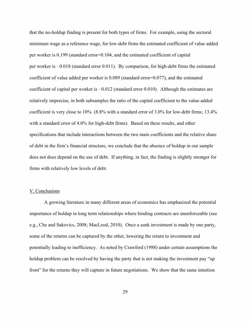
that the no-holdup finding is present for both types of firms. For example, using the sectoral

minimum wage as a reference wage, for low-debt firms the estimated coefficient of value added

per worker is 0.199 (standard error=0.104, and the estimated coefficient of capital

per worker is !0.018 (standard error 0.011). By comparison, for high-debt firms the estimated

coefficient of value added per worker is 0.089 (standard error=0.077), and the estimated

coefficient of capital per worker is !0.012 (standard error 0.010). Although the estimates are

relatively imprecise, in both subsamples the ratio of the capital coefficient to the value-added

coefficient is very close to 10% (8.8% with a standard error of 3.0% for low-debt firms; 13.4%

with a standard error of 4.0% for high-debt firms). Based on these results, and other

specifications that include interactions between the two main coefficients and the relative share

of debt in the firm’s financial structure, we conclude that the absence of holdup in our sample

does not does depend on the use of debt. If anything, in fact, the finding is slightly stronger for

firms with relatively low levels of debt.

V. Conclusions

A growing literature in many different areas of economics has emphasized the potential

importance of holdup in long term relationships where binding contracts are unenforceable (see

e.g., Che and Sakovics, 2008; MacLeod, 2010). Once a sunk investment is made by one party,

some of the returns can be captured by the other, lowering the return to investment and

potentially leading to inefficiency. As noted by Crawford (1988) under certain assumptions the

holdup problem can be resolved by having the party that is not making the investment pay “up

front” for the returns they will capture in future negotiations. We show that the same intuition

30

applies to worker-firm bargaining. We derive an expression for the quasi-rent that is split by the

bargaining parties in each period and show that it deducts the cost of the fraction of the current

capital stock that is fully reversible, plus the cost of the irreversible share of the future capital

stock. The sum of these deductions is approximately equal to the full cost of capital. By

comparison, in the presence of distortionary holdup only a fraction of the cost of the current

capital stock is deducted, and firms have an incentive to under-invest.

We then use a matched employer-employee data set from the Veneto region of Italy that

contains individual earnings records and firm-specific balance sheet data to estimate within-job

models of rent-sharing and test for holdup. We find strong evidence of rent sharing, with an

elasticity of wages with respect to profits on the order of 3-5%, mainly arising from firms in

more concentrated industies. We also find that firms with higher capital per worker pay lower

wages, holding constant value-added per worker. The relative size of the deduction for capital is

consistent with efficient investment (i.e., no holdup) assuming a user cost of capital of around

10%. The deduction is larger for tangible investments than for working capital ! a pattern that is

inconsistent with a higher risk of holdup for tangible investments, but consistent with a lower

user cost for liquid assets. The relative magnitude of the deduction is also similar for firms with

relatively low and relatively high levels of debt, suggesting that the absence of holdup is not

directly attributable to the strategic use of debt financing.

There are a number of limitations of our empirical analysis that need to be kept in mind.

We have no information on the presence of formal firm-level contracts, so our analysis of rent

sharing represents a combination of formal and informal contracting. Our matched data set also

covers a relatively short period (6 years), so we have to rely on the reported book value of

31

capital, rather than on a capital series derived from past investments. Finally, the power of our

instrumental variables strategy is limited and in some specifications the estimated effects of

quasi-rents on wages are rather imprecise. In view of these and other limitations our findings

must be interpreted with some care. Nevertheless, we believe our findings suggest that rent

sharing does not necessarily lead to inefficiently low levels of investment by firms that either

formally or informally share rents with their employees.

32

Appendix A

This appendix derives expressions for wages and other outcomes when employment is set

unilaterally by the firm. As in the simpler cases described in the text, we proceed backward from

the second period. Given K2 and θ2, the second period wage negotiation maximizes

(A1) [ (w!m2)L2 ]γ [ R(L2,K2,θ2) ! wL2 ! δr2K2 ]1!γ ,

where L2 is endogenously determined from the labor demand schedule L2(w2, K2, θ2). Using the

fact that MR(L2,K2,θ2)/ML2 ! w2 = 0, the first-order condition for w2 can be written as:

(A2) (w2 !m2) L2 = γ/(1!γ) × [ 1 + ε (w2 !m2)/w2 ] × [ R(L2, K2, θ2) ! w2L2 ! δr2K2 ] ,

where ε is the elasticity of labor demand, which we assume is constant. Since L2 is endogenous,

we approximate (A2) around L2* = L2(m2, K2, θ2), the efficient employment level in period 2.

We assume that

(A3) L2 . L2* × ( 1 + ε (w2 !m2)/w2 ) ,

and use a first order approximation of the firm’s profit function around the profit associated with

the wage m2:

(A4) R(L2, K2, θ2) ! w2L2 . R(L2*, K2, θ2) ! m2 L2

* ! L2* (w2 !m2) .

Substituting (A3) and (A4) into (A2) we obtain:

(A5) w2 = m2 + γ Q2*/L2

*

where

(A6) Q2* = R(L2

*, K2, θ2) ! m2 L2* ! δr2 K2

is the “efficient” quasi-rent in period 2. The optimized value of the second period bargain to

workers is:

(A7) (w2 !m2) L2 = γ Q2* × L2 /L2

* = γ (1 + ε g2* ) Q2

*

where g2* = (w2 !m2)/w2 = γ Q2

*/(m2 L2* ) is the optimized proportional wage markup. Using

equation (A4), the firm’s second period profits can be written as:

(A8) π2 = R(L2, K2, θ2) ! w2L2 ! δ r2 K2

= Q2* ! L2

* (w2 !m2) ! (1!δ)r2K2

= (1 !γ) Q2* ! (1!δ)r2K2 .

33

Turning now to the first period, the wage w1 is selected to maximize

(A9) [ (w1 !m1)L1 + βγ(1 + εg2* )Q2

* ]γ

× [ R(L1,K1,θ1 ) ! w1L1 ! δr1K1 + β(1!γ)Q2* ! β(1!δ)r2K2 ]1!γ

subject to the condition that the firm selects L1 once the wage is determined. We assume that the

firm selects K2 unilaterally in period 1, anticipating the choice for w1 and w2. The first order

condition for the negotiated first period wage can be written as

(A10) (w1 !m1) L1 + βγ(1 + εg2* )Q2

* = γ/(1!γ) × (1 + ε(w1!m1)/w1 )

× [ R(L1,K1,θ1 ) ! wL1 ! δr1K1 ! β(1!δ) r2 K2 + β(1!γ)Q2* ]

Notice that if

(1 + εg2* ) = (1 + ε (w1!m1)/w1),

then the terms involving Q2* cancel from the both sides of (A10). Since g2

* = (w2 !m2)/w2, this

will be true if the markup of the wage over the outside wage is constant over time (or if ε=0).

Assuming a constant markup, (A10) can be written as

(A11) (w1 !m1) L1 = γ/(1!γ) × (1 + ε (w1 !m1)/w1 )

× [ R(L1,K1,θ1 ) ! wL1 ! δr1K1 ! β(1!δ) r2 K2 ].

This has exactly the same form as (A2) – the first order condition for w2 – and using a similar

first order expansion of the profit function we get

(A12) w1 = m1 + γ Q1*/L1

*

where

(A13) Q1* = R(L1

*, K1, θ1) ! m1 L1* ! δ r1 K1 ! β(1!δ) r2 K2

and L1* = L1(m1, K1, θ1), the efficient employment level in period 1. Note that, as in the

baseline model with fixed employment, the quasi-rent expression deducts a share δ of first period

capital costs, and a (discounted) share (1!δ) of second period costs. Comparing (A12) to (A5),

the markup of the negotiated wage over the outside alternative will be constant if the ratio of

efficient quasi-rent to efficient employment is constant – a situation that we regard as plausible.32

Finally, we turn to the determination of K2, which we assume is made unilaterally by the

firm, anticipating wages over the next two periods. Paralleling (A8), the firm’s first period

32In a 2-period model, the quasi-rent in the second period does not include a discount for future capital costs. In a multi-period model, however, the quasi-rent in successive periods (except the last) will have the form of (A13).

34

profits can be written as

(A14) π1 = (1 !γ) Q1* ! (1!δ) r1 K1 + β(1!δ) r2 K2 .

Thus,

(A15) π1 + βπ2 = (1 !γ) Q1* ! (1!δ) r1 K1 + β(1!δ) r2 K2

+ β(1 !γ) Q2* ! β(1!δ) r2 K2

= (1 !γ) [ Q1* + β Q2

* ] ! (1!δ) r1 K1

which implies that the firm selects a K2 that maximizes the discounted quasi-rent. Using the

definitions of Q1* and Q2

* we obtain:

(A16) Q1* + β Q2

* = R(L1*, K1, θ1) ! m1 L1

* ! δ r1 K1

+ β[ R(L2*, K2, θ2) ! m2 L2

* ! r2 K2 ] .

Thus, the firm’s first order condition for K2 sets MR(L2*, K2, θ2)/MK2 = r2 , implying an efficient

capital choice.

With unilateral employment-setting, L1 will differ from L1*, and the observed level of

quasi-rent for a particular bargaining pair (Q1) will differ from the efficient quasi-rent (Q1*) that

appears in the wage determination model. In particular, the observed quasi-rent implied by the

model is

(A17) Q1 = R(L1, K1, θ1) ! m1 L1 ! r1 δ K1 ! β(1!δ) r2 K2 ,

and, using an first-order expansion like (A4),

(A18) Q1 = R(L1*, K1, θ1) ! m1 L1

* ! r1 δ K1 ! β(1!δ) r2 K2 + (L1 ! L1*)(w1 ! m1)

= Q1* + (L1 ! L1

*)(w1 ! m1) .

Using the approximation that L1 = L1* ( 1 + ε (w1 !m1)/m1 ) and equation (A12) this can be

further simplified to:

(A19) Q1 = Q1* ( 1 + εγg1

* )

where g1* = (w1 !m1)/m1 is the optimal first period markup. Finally, measured quasi-rent per

employee is:

(A20) Q1 / L1 = Q1* ( 1 + εγg1

* ) / [ L1* ( 1 + εg1

* ) ]

. Q1* / L1

* × ( 1 ! εg1*(1!γ) ) > Q1

* / L1* .

Thus, measured quasi-rent per worker overstates Q1* / L1

*, the measure of quasi-rent per worker

that drives wage determination, by approximately |ε| g1*(1!γ) percent.

35

References

Abowd, John M. and Thomas Lemieux (1993). “The Effects of Product Market Competition on Collective Bargaining Agreements: The Case of Foreign Competition in Canada.” Quarterly Journal of Economics 108, pp. 983–1014. Abowd, John M., Francis Kramarz, and David N. Margolis. (1999) “High-Wage Workers and High-Wage Firms.” Econometrica, 67(2), pp. 251-333. Addison, John T. and Barry T. Hirsch (1989) “Union Effects on Productivity, Profits, and Growth: Has the Long Run Arrived?" Journal of Labor Economics 7, pp. 72-105. Arachi, Giampaolo and Federico Biagi (2005). “Taxation, Cost of Capital, and Investment: Do Tax Asymmetries Matter? Gionale degli Economisti e Annali di Economia 64 (2/3), pp. 295-322. Arai, Mahmood. (2003) “Wages, Profitability and Capital Intensity: Evidence from Matched Worker-Firm Data.” Journal of Labor Economics 21 (3), pp. 593-618. Arai, Mahmood, and Fredrik Heyman. (2004). “Microdata Evidence on Rent-Sharing.” FIEF Working Paper No. 198. Stockholm: Trade Union Institute for Economic Research (FIEF). Baldwin, Carliss (1983). “Productivity and Labor Unions: An Application of the Theory of Self-Enforcing Contracts.” Journal of Business 56, pp. 155-186. Becker, Gary S. (1962). “Investment in Human Capital: A Theoretical Analysis.” Journal of Political Economy 70 (Supplement), pp. 9-49. Blanchflower, David G., Andrew J. Oswald, and Peter Sanfey (1996). “Wages, Profits and Rent-sharing.” Quarterly Journal of Economics 111 , pp. 227–251. Brander James and Tracy Lewis (1986). “Oligopoly and Financial Structure: The Limited Liability Effect.” American Economic Review 76 , pp. 956-970. Bronars, Stephen G. and Donald R. Deere (1993) “Unionization, Incomplete Contracting, and Capital Investment.” Journal of Business; 66(1), pp. 117-32. Brown, James N. and Orley Ashenfelter (1986). “Testing the Efficiency of Employment Contracts.” Journal of Political Economy 94 (3, Supplement), pp, pp. S40-S87. Casadio Piero (2003), “Wage Formation in the Italian Private Sector After the 1992–93 Income Policy Agreements.” In G. Fagan, F.P. Mongelli and J. Morgan, editors, Institutions and Wage Formation in the New Europe, Cheltenham, UK: Edward Elgar, pp. 112–33. Che, Yeon-Koo and Jozsef Sakovics (2008). "Hold-up Problem." In Steven N. Durlauf and Lawrence E. Blume, editors, The New Palgrave Dictionary of Economics, Second Edition. New

36

York: Palgrave Macmillan. Cristini, Annalisa and Riccardo Leoni (2006). “The ′93 July Agreement in Italy: Bargaining Power, Efficiency Wages, or Both?” In Nicola Acocella and Riccardo Leoni, editors, Social Pacts, Employment and Growth: A Reappraisal of Ezio Tarantelli’s Thought. Heidelberg: Physica-Verlag. pp. 97-122. Christofides, Louis N. and Andrew J. Oswald (1992). “Real Wage Determination and Rent-sharing in Collective Bargaining Agreements.” Quarterly Journal of Economics 107, pp. 985–1002. Connolly, Robert A., Barry T. Hirsch, and Mark Hirschey (1986). “Union Rent Seeking, Intangible Capital, and Market Value of the Firm.” Review of Economics and Statistics 68 (4) pp. 567-577. Crawford, Vincent F. (1988). “Long-Term Relationships Governed by Short-Term Contracts.” American Economic Review 78 (3), pp. 485-499 . Cahuc, Pierre and André Zylberberg (2004). Labor Economics. Cambridge MA: MIT Press. Dasgupta, Sudipto and Kunal Sengupta (1993). “Sunk Investment, Bargaining, and the Choice of Capital Structure.” International Economic Review 34 (1), pp. 203-220. Dell'Aringa, Carlo, and Claudio Lucifora. (1994). “Collective Bargaining and Relative Earnings in Italy.” European Journal of Political Economy, Vol. 10, pp. 727–47. de Menil, George (1971). Bargaining: Monopoly Power versus Union Power. Cambridge, MA: MIT Press Denny, Kevin and Stephen J. Nickell (1992). “Unions and Investment in British Manufacturing Industry.” British Journal of Industrial Relations 29 (1), pp. 113-121. Dickens, William T. and Lawrence F. Katz (1986) “Industry Wage Patterns and Theories of Wage Determination.” Unpublished Manuscript, University of California at Berkeley. Elston, Julie Ann and Laura Rondi (2006). “Shareholder Protection and the Cost of Capital: Empirical Evidence from German and Italian Firms.” CERIS-CNR Working Paper No. 8. Montcalieri (Italy): CERIS-CNR. Franzosi, Alessandra M. (2008). “Costo del Capitale e Struttura Finanziaria: Valutazione degli Effecti di IRAP e DIT.” Instituto per la Ricerca Sociale (Milano) Unpublished Working Paper. Grout, Paul A. (1984). “Investment and Wages in the Absence of Binding Contracts: A Nash Bargaining Approach.” Econometrica 52 (2), pp. 449-460.

37

Guiso, Luigi, Luigi Pistaferri and Fabiano Schivardi (2005). “Insurance within the Firm.” Journal of Political Economy 113 (5), pp. 1054-1087. Guertzgen, N. (forthcoming). “Rent-Sharing and Collective Wage Contracts - Evidence from German Establishment-Level Data.” Forthcoming in Applied Economics. Hildreth, A.K.G. and Andrew J. Oswald (1997). “Rent-sharing and Wages: Evidence from Company and Establishment Panels.” Journal of Labor Economics 15, pp. 318–337. Hirsch, Barry T. (2004). “What Do Unions Do For Economic Performance?” Journal of Labor Research 25, pp. 417-455. Istat (2000). “La FlessibilitB del Mercato del Lavoro nel Periodo 1995-96.” Informazioni 34 Roma: ISTAT. Lester, Richard A. (1952). “A Range Theory of Wage Differentials.” Industrial and Labor Relations Review 5, pp. 483-500. Machin, Stephen and Sushil Wadhwani (1991). “The Effects of Unions on Investment and Innovation: Evidence From WIRS.” Economic Journal 101 (405), pp. 324-330. MacLeod, W. Bentley (2010). “Great Expectations: Law, Employment Contracts, and Labor Market Performance.” In Orley Ashenfelter and David Card, editors, Handbook of Labor Economics Volume 4. New York: Elsevier, forthcoming 2010. Manning, Alan (1987). “An Integration of Trade Union Models in a Sequential Bargaining Framework.” Economic Journal 97 (385), pp. 121-139. Margolis, David N. and Kjell G. Salvanes. (2001). “Do Firms Really Share Rents with Their Workers?” IZA Discussion Paper No. 330. Bonn: IZA. Martins, Pedro (2009) “Rent Sharing Before and After the Wage Bill.” Applied Economics 41 (17), pp. 2133-2151. McDonald, Ian M., and Robert Solow (1981). “Wage Bargaining and Employment.” American Economic Review 71, pp. 896-908. Myers, Stewart (1977). “The Determinants of Corporate Borrowing.” Journal of Financial Economics 4, pp. 147-175. Nickell, Stephen J. and Sushil Wadhwani (1990). “Insider Forces and Wage Determination.” Economic Journal 100(401), pp. 496-509. Simons, Henry (1944). “Some Reflections on Syndicalism.” Journal of Political Economy 52, pp. 1-25.

38

Slichter, Sumner. (1950). “Notes on the Structure of Wages. Review of Economics and Statistics 32, pp. 80–91. Smith, Adam. (1976). An Enquiry into the Nature and Causes of the Wealth of Nations, Clarendon Press, Oxford. Subramaniam, Venkat (1996). “Underinvestment, Debt Financing, and Long-Term Supplier Relations.” Journal of Law, Economics and Organizations 12 (2), pp. 461-475. Svejnar, Jan. (1986). “Bargaining Power, Fear of Disagreement, and Wage Settlements: Theory and Evidence from U.S. Industry.” Econometrica 54 (5), pp. 1055-1078. Tattara, Giuseppe and Marco Valentini (2007). “The Cyclical Behavior of Job and Worker Flows.” Working Paper No. 16. Department of Economics Ca’ Foscari University of Venice. Usman, Murat. (2004). “Optimal Debt Contracts with Renegotiation.” Journal of Economics and Management Strategy 13 (4), pp. 755-776. Van Reenen, John. (1996). "The Creation and Capture of Economic Rents: Wages and Innovation in a Panel of UK Companies" Quarterly Journal of Economics 111 (443), pp. 195-226.

Table 1: Descriptive Statistics for Workers, Firms and Job Matches

Universe of Matched Estimation SampleJob-Year Job-Year Subset Matched to

Observations Observations Full Sample Sectoral Contract(1) (2) (3) (4)

Characteristics of Workers:1. Number of Individual Workers 1,990,751 985,160 416,587 305,364

2. Percent Female 42.3 34.4 27.3 26.8

3. Percent Age 30 or Less 45.6 39.8 41.3 42.5

4. Percent Age 45 or More 17.1 19.8 18.1 17.4

5. Percent White Collar 29.6 29.8 31.3 32.9

6. Mean Daily Wage (real Euros) 64.8 74.2 68.9 68.37

7. Mean Drift Component of Daily Wage − − − 21.2 (real Euros)

Characteristics of Firms:8. Number of Individual Firms 191,202 18,312 7,283 5,677

9. Firm Size a 7.0 36.0 54.4 54.8

10. Value Added/Worker (1000's real Euros) − 59.7 44.6 44.5

11. Valued Added/Worker less Industry Mean Wage − 31.5 24.4 20.1 (1000's of real Euros)

12. Valued Added/Worker less Sectoral Min. Wage − − − 30.2 (1000's of real Euros)

13. Quasi-rent/Worker, using Industry Mean Wage − 23.3 20.0 20.1 (1000's of real Euros)

14. Quasi-rent/Worker, using Sectoral Min. Wage − − − 26.2 (1000's of real Euros)

Characteristics of Job Match:15. Number of Job Matches 3,111,990 1,223,889 452,136 328,824

16. Mean Duration of Job (years) 2.1 2.5 3.5 3.5

aIn column 1 firm size is based on number of employees as of October in VWH data. In other columns firm size is from AIDA data.

Notes: Sample in column 1 includes observed jobs for individuals between the ages of 16 and 64 in Veneto Worker History File during a calendar year between 1995 and 2001. Sample in column 2 includes subset of job-year observations that can be matched to AIDA balance sheet data for the firm (in the same calendar year). Estimation sample excludes part-year jobs, jobs at firms with under 15 employees, part-time jobs, jobs held by apprentices and managers, and jobs in construction and sectors with a relatively small number of AIDA firms outside Veneto. Sample in column 4 includes job-year observations that can be matched to information on the minimum wage in the relevant sectoral contract. See text for further details.

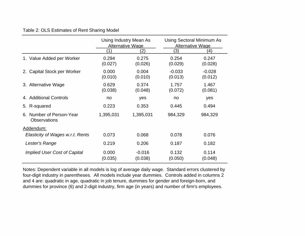
Table 2: OLS Estimates of Rent Sharing Model

(1) (2) (3) (4)1. Value Added per Worker 0.294 0.275 0.254 0.247 (0.027) (0.026) (0.029) (0.028)

2. Capital Stock per Worker 0.000 0.004 -0.033 -0.028(0.010) (0.010) (0.013) (0.012)

3. Alternative Wage 0.629 0.374 1.757 1.467(0.038) (0.048) (0.072) (0.081)

4. Additional Controls no yes no yes

5. R-squared 0.223 0.353 0.445 0.494

6. Number of Person-Year 1,395,031 1,395,031 984,329 984,329 Observations

Addendum: Elasticity of Wages w.r.t. Rents 0.073 0.068 0.078 0.076 Lester's Range 0.219 0.206 0.187 0.182

Implied User Cost of Capital 0.000 -0.016 0.132 0.114(0.035) (0.038) (0.050) (0.048)

Using Industry Mean As Alternative Wage

Using Sectoral Minimum As Alternative Wage

Notes: Dependent variable in all models is log of average daily wage. Standard errors clustered by four-digit industry in parentheses. All models include year dummies. Controls added in columns 2 and 4 are: quadratic in age, quadratic in job tenure, dummies for gender and foreign-born, and dummies for province (6) and 2-digit industry, firm age (in years) and number of firm's employees.

Table 3: OLS and IV Within-Spell Estimates of Rent Sharing Model

OLS IV OLS IV(1) (2) (3) (4)

1. Value Added per Worker 0.032 0.117 0.030 0.146(0.005) (0.062) (0.007) (0.071)

2. Capital Stock per Worker -0.002 -0.012 -0.002 -0.015(0.003) (0.007) (0.003) (0.008)

3. Alternative Wage 0.011 0.010 0.801 0.800(0.009) (0.007) (0.035) (0.029)

4. Additional Controls yes yes yes yes

5. Number of Person-Year 1,395,301 1,395,301 984,329 984,329 Observations

6. First-stage F-statistic − 28.2 − 20.3

Addendum: Elasticity of Wages w.r.t. Rents 0.008 0.029 0.009 0.045 Lester's Range 0.024 0.087 0.022 0.108

Implied User Cost of Capital 0.074 0.107 0.058 0.105(0.098) (0.025) (0.111) (0.023)

Using Industry Mean As Alternative Wage

Using Sectoral Minimum As Alternative Wage

Notes: Dependent variable in all models is log of average daily wage. All models include a complete set of job-spell dummies as well as year effects and the covariates described in Table 2 that vary within job spells. In IV models (columns 2 and 4) value-added per worker is treated as endogenous. Instrument is revenue per worker for firms in the same 4 digit industry in the same year in other regions of Italy. Standard errors clustered by four digit industry in parentheses.

Table 4: IV Within-Spell Estimates of Rent Sharing Model, Treating Capital as Endogenous

(1) (2)

1. Value Added per Worker 0.153 0.147(0.081) (0.105)

2. Capital Stock per Worker -0.038 -0.030(0.009) (0.012)

3. Alternative Wage 0.009 0.790(0.008) (0.034)

4. Additional Controls yes yes

5. Number of Person-Year 1,127,153 806,348 Observations

6. First-stage F-statistic for 13.9 10.4 Value added per Worker

7. First-stage F-statistic for 77.5 64.7 Capital Stock per Worker

Addendum: Elasticity of Wages w.r.t. Rents 0.038 0.045 Lester's Range 0.111 0.105

Implied User Cost of Capital 0.251 0.203(0.122) (0.119)

Using Sectoral Minimum As Alternative Wage

Notes: Dependent variable in both models is log of average daily wage. Models include a complete set of job-spell dummies as well as year effects and the covariates described in Table 2 that vary within job spells. Value-added per worker and capital per worker are treated as endogenous. Instruments are revenue per worker for firms in the same 4 digit industry in the same year in other regions of Italy, and lagged capital per worker at the firm. Standard errors clustered by four-digit industry in parentheses.

Using Industry Mean As Alternative Wage

Table 5: IV Within-Spell Estimates of Rent Sharing Model, Distinguishing Three Types of Capital

(1) (2)

1. Value Added per Worker 0.120 0.154(0.074) (0.080)

2. Tangible Fixed Assets per Worker -0.011 -0.013 (plant and equipment) (0.007) (0.007)

3. Intangible Fixed Assets per Worker -0.027 -0.033 (intellectual property, R&D, goodwill) (0.013) (0.017)

4. Current Assets per Worker -0.003 -0.005 (inventories, receiveables, non-fixed (0.007) (0.008) financial assets, liquid funds)

5. Alternative Wage 0.010 0.801(0.006) (0.029)

6. Additional Controls yes yes

7. Number of Person-Year 1,395,301 984,329 Observations8. First-stage F-statistic 22.8 17.0 Value added per worker

Addendum: Elasticity of Wages w.r.t. Rents 0.030 0.047 Lester's Range 0.090 0.113

Implied User Cost - Tangible Fixed Assets 0.092 0.087(0.025) (0.024)

Implied User Cost - Intangible Fixed Assets 0.225 0.217(0.134) (0.114)

Implied User Cost - Current Assets 0.021 0.035(0.047) (0.032)

Using Sectoral Minimum As Alternative Wage

Notes: Dependent variable in both models is log of average daily wage. Models include a complete set of job-spell dummies as well as year effects and the covariates described in Table 2 that vary within job spells. Value-added per worker is treated as endogenous. Instrument is revenue per worker for firms in the same 4 digit industry in the same year in other regions of Italy. Standard errors clustered by four-digit industry in parentheses.

Using Industry Mean As Alternative Wage

Table 6: IV Within-Spell Estimates of Rent Sharing Model for Different Sectors

Non High Low All High K/L Low K/L Manufacturing Concentration Concentration

(1) (2) (3) (4) (5) (6)

1. Value Added per Worker 0.207 0.259 0.254 0.084 0.233 0.012(0.097) (0.164) (0.121) (0.079) (0.111) (0.085)

2. Capital Stock per Worker -0.021 -0.028 -0.024 -0.010 -0.024 -0.001(0.011) (0.018) (0.015) (0.010) (0.012) (0.011)

3. Alternative Wage 0.789 0.761 0.811 0.814 0.776 0.816 (Sectoral Minimum) (0.036) (0.058) (0.041) (0.052) (0.042) (0.036)

4. Additional Controls yes yes yes yes yes yes

5. Number of Person-Year 717,674 328,731 388,943 266,655 481,752 502,577 Observations

6. First-stage F-statistic 14.2 5.2 10.7 10.8 10.9 17.6 Value added per worker

Addendum: Elasticity of Wages w.r.t. Rents 0.063 0.079 0.078 0.026 0.071 0.004 Lester's Range 0.152 0.191 0.187 0.062 0.171 0.009

Implied User Cost of Capital 0.102 0.108 0.093 0.123 0.104 0.120(0.027) (0.033) (0.034) (0.047) (0.026) (0.331)

ManufacturingManufacturing versus Other Industries: By Industry Herfindahl:

Notes: Dependent variable in all models is log of average daily wage. Models include a complete set of job-spell dummies as well as year effects and the covariates described in Table 2 that vary within job spells. Value-added per worker is treated as endogenous. Instrument is revenue per worker for firms in the same 4 digit industry in the same year in other regions of Italy. Manufacturing firms are classified as having high or low capital per worker (K/L) if their ratio of capital per worker is above or below the median for all manufacturing firms. High/low concentration classification in columns 5-6 is based on Herfindahl index of sales for 4-digit industry in all of Italy. Standard errors clustered by four-digit industry in parentheses.