natural amenities and tourism employment: a spatial analysis

i

Natural Amenities and Tourism Employment: A

Spatial Analysis

Dhammika Niromi Naranpanawa BSc. MSc. MEnvSc.

A thesis submitted for the degree of

Doctor of Philosophy at

The University of Queensland

2019

School of Earth and Environmental Sciences

iii

Abstract

This thesis examines the spatial linkages between natural amenities and tourism

employment when spatial spillover effects are taken into account under three neighbourhood

structures. To the author’s knowledge, tourism employment and natural amenity spillovers

have not previously been examined in a non-geographic spatial context.

To address this research gap and explore the non-geographic spatial spillovers in

tourism employment and natural amenities, spatial models are developed with different

neighbourhood structures. In addition, the thesis examines: tourism clusters; the

measurement of cluster proximity; and characteristics of tourism employment within and

across clusters.

This thesis developed an empirical model at the local government level for

Queensland, Australia. The model incorporates 13 natural amenity variables and four other

variables that explain regional tourism employment. The analysis is conducted for 74 local

governments in Queensland using cross-sectional data compiled for 2011.

Three specifications of a Spatial Durbin Model (SDM) are implemented. The

specifications use three alternative weight matrices to reflect three different proximity

dimensions or neighbourhood structures. A non-spatial linear model (NSLM) estimated by

least squares is used as the base model. The three weight matrices specifications are

proportional to: a) geographic contiguity, to capture geographic spillovers; b) the share of

employment in the tourism industry; and c) the proportion of tourism employment to total

employment. The last two are measures of economic distance.

To identify tourism employment clusters, the study uses a K-mean cluster analysis

technique. Factor analysis is used to summarise 17 variables selected from a review of

theoretical models of tourism employment. Based on computed factor scores, the main

cluster attributes are identified.

The results suggest that independent of the specification (spatial and non-spatial),

internet penetration, regional population, the number of regional parks and state forests and

World Heritage areas are statistically significant. This is taken as evidence of their

importance as factors that influence tourism employment in a region. Most importantly,

spillovers exist; not only between traditional geographic neighbours, but also between

neighbours of economic proximity where neighbours are those that have a similar profile in

their share of tourism employment.

iv

When the spatial autocorrelation parameter is negative and significant between

geographic neighbours, it reflects competition; however, when it is positive and significant

between economic neighbours (regions with similar share of tourism employment) it

indicates a collaborative effect between the regions with similar tourism performance. The

results further suggest non-geographic proximity can explain tourism employment clusters.

Characteristics such as “urbanness”, communications capacity, natural attractions, level of

agriculture and percentage of indigenous population are shared within clusters.

The conclusion is that non-geographical proximity dimensions can be highly

informative when developing plans or strategies to maximise spillovers and clustering in

regional tourism.

v

Declaration by author

This thesis is composed of my original work, and contains no material previously

published or written by another person except where due reference has been made in the

text. I have clearly stated the contribution by others to jointly-authored works that I have

included in my thesis.

I have clearly stated the contribution of others to my thesis as a whole, including

statistical assistance, survey design, data analysis, significant technical procedures,

professional editorial advice, financial support and any other original research work used or

reported in my thesis. The content of my thesis is the result of work I have carried out since

the commencement of my higher degree by research candidature and does not include a

substantial part of work that has been submitted to qualify for the award of any other degree

or diploma in any university or other tertiary institution. I have clearly stated which parts of

my thesis, if any, have been submitted to qualify for another award.

I acknowledge that an electronic copy of my thesis must be lodged with the University

Library and, subject to the policy and procedures of The University of Queensland, the thesis

be made available for research and study in accordance with the Copyright Act 1968 unless

a period of embargo has been approved by the Dean of the Graduate School.

I acknowledge that copyright of all material contained in my thesis resides with the

copyright holder(s) of that material. Where appropriate I have obtained copyright permission

from the copyright holder to reproduce material in this thesis and have sought permission

from co-authors for any jointly authored works included in the thesis.

vi

Publications included in this thesis

No publications included

Submitted manuscripts included in this thesis

No manuscripts submitted for publication

Other publications during candidature

Niromi Naranpanawa, Alicia N. Rambaldi and Neil Sipe, ‘Natural amenities and Tourism

Employment: A Spatial Analysis’, Papers in Regional Science (2019).

Contributions by others to the thesis

No contributions by others

Statement of parts of the thesis submitted to qualify for the

award of another degree

No works submitted towards another degree have been included in this thesis

Research Involving Human or Animal Subjects

No animal or human subjects were involved in this research

vii

Acknowledgements

I would like to begin by expressing my absolute deepest gratitude and respect to my

supervisors, Professor Neil Sipe and Professor Alicia Rambaldi, who have supported me

endlessly throughout my PhD journey with their profound intellectual contribution and

constant encouragement. If it were not for their continuous guidance and support, this thesis

would not have been possible. In particular, I wish to express my sincere indebtedness to

Neil for his optimism, patience, encouragement and overall guidance to make my PhD a

success. My deepest gratitude goes to Alicia, my associate supervisor, who was willing to

share her strong intellectual understanding in spatial econometric modelling with me during

the study period. I am deeply grateful for her guidance in constructing my spatial

econometric models, which are the major contribution of my thesis. Thank you both so much

for your encouragement.

I wish to express my sincere thanks to the University of Queensland for granting me a

University of Queensland Research Scholarship to conduct my research studies that lead

to my PhD at the University of Queensland.

I am deeply thankful to Dr Sally Driml for giving me an opportunity to work at the end

of my scholarship period which helped me to overcome my financial stresses. I would like

to thank Dr Tien Pham for his valuable advice particularly on estimating tourism

employment. My sincere thanks also go to Professor Rodney Wolff for his valuable guidance

at the early stages of my research. My sincere thanks go to Jurgen Overheu for his technical

support and Catriona McLeod for editorial support. I would like to thank my friends, who have

given me a heaps of wonderful times which helped me to have a life-study balance and let

go my stress during my study period.

My greatest appreciation goes to my dear parents, Duleep and Eunice Gooneratne, for

their selfless support through my entire life. My father’s positive attitudes and great

encouragement are truly admirable. Finally my heartiest thanks go to my husband Athula,

son Rajitha, and daughter Sachini for their continuous patience, love and care during this

long and tiring journey of completion of my research work.

viii

Financial support

This research was supported by a University of Queensland Research Scholarship

Keywords

Tourism employment, natural amenity, regional tourism, geographic proximity, non-

geographic proximity, spatial analysis, factor analysis, cluster analysis, spatial econometric

model

Australian and New Zealand Standard Research Classifications

(ANZSRC)

ANZSRC code: 160402, Recreation Leisure and Tourism Geography, 50%

ANZSRC code: 140216, Tourism Economics, 50%

Fields of Research (FoR) Classification

FoR code: 1604 Human Geography, 50%

FoR code: 1402 Applied Economics, 50%

ix

Dedication

To my loving parents

Who believe in the

Richness of Learning

x

Table of Contents

Abstract .......................................................................................................................................... iii

Declaration by author ...................................................................................................................... v

Publications during candidature ...................................................................................................... vi

Publications included in this thesis ................................................... Error! Bookmark not defined.

Contributions by others to the thesis ............................................................................................... vi

Statement of parts of the thesis submitted to qualify for the award of another degree ..................... vi

Acknowledgements ........................................................................................................................ vii

Dedication ....................................................................................................................................... ix

Table of Contents............................................................................................................................ x

List of Figures .............................................................................................................................. xvii

List of Tables .............................................................................................................................. xviii

Chapter 1 ........................................................................................................................................ 1

Introduction ..................................................................................................................................... 1

1.1 Background, the problem and research rationale .................................................................. 1

1.2 Research approach and the thesis framework ....................................................................... 5

1.3 Aims of the study ................................................................................................................... 5

1.4 Research objectives .............................................................................................................. 8

1.4.1 Research Objective 1 ...................................................................................................... 8



1.5 Research Questions .............................................................................................................. 9

1.5.1 Research Question 1 ...................................................................................................... 9



1.6 Contribution to literature ...................................................................................................... 10

1.7 Thesis structure ................................................................................................................... 10

Chapter 2 ...................................................................................................................................... 13

Literature review ........................................................................................................................... 13

Natural amenities, regional tourism and regional economies ........................................................ 13

2.1 Introduction.......................................................................................................................... 13

2.2. Structural changes in regional economies and changes in perceptions of the role of natural

resources in regional economies ............................................................................................... 15

2.3 Natural amenity ................................................................................................................... 15

2.3.1 Defining natural amenities ............................................................................................. 16

2.3.2 Values of natural amenity .............................................................................................. 16

xi

2.3.3 Characteristics of natural amenity ................................................................................. 17

2.3.4 Measuring natural amenity attributes ............................................................................ 17

2.3.5 List of amenity variables ................................................................................................ 18

2.3.6 Summary index approach (Single dimension) ............................................................... 18

2.3.7 Aggregate Factor Score Approach ................................................................................ 18

2.4 Theories of regional economic dynamics: jobs versus people or jobs versus amenity ......... 19

2.4.1 New Economic Geography (NEG) ................................................................................. 19

2.4.2 Amenity-led growth: jobs follow amenity ........................................................................ 19

2.5 The role of natural amenities in regional development ......................................................... 20

2.6 Natural amenities in rural development through population growth due to in-migration ........ 21

2.6.1. Natural amenities and rural development through employment including tourism

employment ........................................................................................................................... 23

2.6.2 Natural amenity, income distribution and inequality and per capita income ................... 24

2.7 Spatial dependence of natural amenities ............................................................................. 25

2.8 Tourism ............................................................................................................................... 27

2.8.1 Background ................................................................................................................... 27

2.8.2 Definitions and interpretations of tourism ...................................................................... 28

2.9 Theoretical perspectives of tourism ..................................................................................... 30

2.9.1 The framework of tourism as an open system: general system theory and tourism ....... 30

2.9.2 Jafari’s four platforms of tourism research ..................................................................... 30

2.9.3 Advocacy Platform ........................................................................................................ 31

2.9.4 Cautionary Platform ...................................................................................................... 32

2.9.5 Adaptancy Platform ....................................................................................................... 32

2.9.6 Knowledge-based Platform ........................................................................................... 32

2.10 This study in terms of Jafari’s four platforms ...................................................................... 33

2.11 Tourism in natural areas (nature-based tourism) ............................................................... 34

2.11.1 Nature Based Tourism (NBT) ...................................................................................... 34

2.11.2 Working definition of NBT ............................................................................................ 35

2.11.3. Experiences of natural amenities in NBT .................................................................... 36

2.12 A Conceptual framework of nature-based tourism and regional economies ....................... 36

2.13 Approaches to measuring tourism activity.......................................................................... 39

2.13.1 Tourism employment ................................................................................................... 39

2.13.2 Measuring tourism employment .................................................................................. 41

2.14 Summary ........................................................................................................................... 43

Chapter 3 ...................................................................................................................................... 45

An overview of tourism in Queensland .......................................................................................... 45

3.1 Introduction.......................................................................................................................... 45

xii

3.2 The economic significance of tourism .................................................................................. 46

3.3 Tourism 2020 Strategy and Forecasts ................................................................................. 47

3.4 Queensland tourism and the Queensland economy ............................................................ 49

3.4.1 Economic significance of the Queensland tourism industry ........................................... 50

3.5 Tourism Workforce .............................................................................................................. 51

3.6 Regional tourism ................................................................................................................. 53

3.6.1 Queensland tourism destination regions ....................................................................... 53

3.7 The regional economic contribution of tourism in Queensland ............................................. 55

3.7.1 Tropical North Queensland (TNQ) ................................................................................. 56

3.7.2 Northern (Townsville) Region ........................................................................................ 56

3.7.3 Outback Region ............................................................................................................ 56

3.7.4 Whitsundays Region ..................................................................................................... 57

3.7.5 Mackay Region ............................................................................................................. 57

3.7.6 Brisbane Region ........................................................................................................... 57

3.7.7 Southern Great Barrier Reef and Bundaberg North Burnett Region .............................. 58

3.7.8 Central Queensland Region .......................................................................................... 58

3.7.9 Southern Queensland Country (Darling Downs) ............................................................ 58

3.7.10 Gold Coast region ....................................................................................................... 58

3.7.11 Sunshine Coast Region............................................................................................... 59

3.7.12 Fraser Coast Region ................................................................................................... 59

3.8 Natural amenities and tourism in Queensland ..................................................................... 59

3.9 NBT in Queensland ............................................................................................................. 60

3.10 Economic significance of NBT ........................................................................................... 61

3.11 Natural amenities in Queensland ....................................................................................... 61

3.11.1 World Heritage areas: ................................................................................................. 61

3.11.2 Green areas in Queensland ........................................................................................ 63

3.11.3 Ramsar (internationally important) and Nationally important (DIWA) wetlands ............ 63

3.12 Summary ........................................................................................................................... 64

Chapter 4 ...................................................................................................................................... 66

Spatial econometric models to capture geographical as well as non-geographical spillovers in

tourism employment ...................................................................................................................... 66

4.1 Introduction.......................................................................................................................... 66

4.1.1 Motivation ..................................................................................................................... 67

4.2 Literature Review of tourism spillovers and the spatial models with geographic and non-

geographic neighbourhood structures ....................................................................................... 68

4.2.1 Spatial dependence in tourism (tourism spillovers) ....................................................... 68

4.2.2 Spatial dependence in non- geographical neighbourhood structures ............................ 71

xiii

4.3 Research methods .............................................................................................................. 75

4.3.1 Estimating tourism related employment: measuring tourism activity .............................. 75

4.4. Methodology of spatial models ........................................................................................... 77

4.4.1 Introduction ................................................................................................................... 77

4.4.2 The Model: spatial econometric model – spatial dependence ....................................... 78

4.4.3 Types of spatial dependence ........................................................................................ 79

4.4.4 Spatial weight matrices ................................................................................................. 80

4.5 Testing for spatial dependence: statistical tests to examine the presence of spatial

dependence .............................................................................................................................. 84

4.5.1 Lagrange multiplier tests (LM test) ................................................................................ 84

4.5.2 Moran’s I test ................................................................................................................ 85

4.6 Why the SDM model? (Selecting the appropriate spatial model) ......................................... 85

4.6.1 SDM model and explanation of the model ..................................................................... 85

4.7 Interpretation of the model: the parameter estimates ........................................................... 86

4.7.1 Direct, indirect and total effects ..................................................................................... 87

4.8 Estimation method ............................................................................................................... 89

4.9 Model specification and data description ............................................................................. 89

4.9.1 The spatial scale: defining the region ............................................................................ 89

4.10 Selection of variables, data description and data transformation ....................................... 90

4.10.1 The dependent variable: log of tourism employment ................................................... 90

4.11 Explanatory variables ........................................................................................................ 92

4.11.1 Natural amenity variables ............................................................................................ 93

4.12 Control variables................................................................................................................ 97

4.12.1 Estimated resident population (POP) .......................................................................... 97

4.12.2 Urbanness (URBAN) ................................................................................................... 97

4.12.3 Communication and transportation infrastructure variables ......................................... 98

4.13 A variable to capture mining performance of the region ..................................................... 98

4.14 Summary ........................................................................................................................... 99

Chapter 5 .................................................................................................................................... 101

Results of the spatial and non-spatial analysis 2011 ................................................................... 101

5.1 Introduction........................................................................................................................ 101

5.2 Compilation (estimated) tourism employment for LGAs in Queensland ............................. 101

5.3 Normality test for Logarithmic Tourism Employment .......................................................... 103

5.4 Estimation of spatial spillovers in tourism employment and natural amenities .................... 104

5.4.1 The models ................................................................................................................. 104

5.4.2 Results of the hierarchical regression.......................................................................... 105

5.4.3 Diagnostic tests: examining the spatial dependence ................................................... 105

xiv

5.4.4 Parameter estimates of the models ............................................................................. 106

5.4.5 Significance of the spatial correlation parameter (ρ) .................................................... 108

5.4.6 Point estimates ........................................................................................................... 108

5.4.7 Spatial spillover ........................................................................................................... 109

5.5 Direct, indirect and total effects .......................................................................................... 110

5.5.1 Decomposition of spatial effects of the explanatory variables into direct, indirect and total

effects .................................................................................................................................. 110

5.6 Model 2: Spatial model with geographically weighted contiguity matrix .............................. 112

5.6.1 Direct, indirect and total effects ................................................................................... 112

5.6.2 Marginal effects ........................................................................................................... 112

5.7 Model 3: neighbourhood structure based on share of tourism employment ....................... 115

5.7.1 Direct, indirect and total effects ................................................................................... 115

5.8 Comparison of Models 2 and 3 .......................................................................................... 118

5.9 Model 4: Direct, indirect and total effects – neighbourhood structure based on percentage of

total employment ..................................................................................................................... 122

5.10 Prediction of tourism employment .................................................................................... 123

5.11 Robustness of the model under different neighbourhood structure .................................. 123

5.12 Impact of mining on regional tourism in 2011 ................................................................... 124

5.13 Significance of the spatial auto correlation parameter (ρ) ................................................ 125

5.14 Parameter estimates of the models with the mining variable ........................................... 127

5.15 Significance of the mining variable .................................................................................. 127

5.15.1 Model 2M .................................................................................................................. 127

5.15.2 Model 3M .................................................................................................................. 128

5.15.3 Model 4M .................................................................................................................. 128

5.16 Conclusions ..................................................................................................................... 129

Chapter 6 .................................................................................................................................... 132

Identifying proximity dimensions or neighbourhood structures in tourism employment clusters ... 132

6.1 Introduction........................................................................................................................ 132

6.2 Literature review: background............................................................................................ 133

6.3 Theoretical foundation of clusters ...................................................................................... 134

6.3.1 The New Economic Geography (NEG) ........................................................................ 134

6.3.2 Cluster theory: Clusters based on geographic proximity .............................................. 134

6.4 Other proximity dimensions for clusters ............................................................................. 136

6.5 The application of clustering and proximity dimensions in tourism ..................................... 137

6.6 Research method .............................................................................................................. 139

6.7 Step 1: Identification of clusters based on tourism employment, using cluster analysis ..... 139

6.7.1 Cluster analysis ........................................................................................................... 140

xv

6.7.2 K-mean clustering ....................................................................................................... 140

6.7.3 Proximity distance: assigning items to the closest centroid ......................................... 141

6.7.4 The choice of number of clusters and the clustering method ....................................... 141

6.8 Step 2: Identification of the underlying attributes of the clusters......................................... 142

6.8.1 Constructing factors using EFA ................................................................................... 142

6.8.2 Exploratory factor analysis (EFA) ................................................................................ 142

6.8.3 The Factor Model: the orthogonal factor model ........................................................... 145

6.8.4 Estimation factor scores .............................................................................................. 146

6.9 Empirical Results ............................................................................................................... 147

6.9.1 Identifying the clusters based on estimated tourism employment ................................ 147

6.9.2 Identification of the factors and the factor scores ........................................................ 148

6.9.3 Results of initial selected factors ................................................................................. 148

6.10 Estimating factor scores .................................................................................................. 152

6.11 Attributes of clusters based on factor scores derived from the selected variables and to

define the proximity dimension inherent to each cluster ........................................................... 152

6.12 Conclusions ..................................................................................................................... 156

Chapter 7 .................................................................................................................................... 157

Summary and Conclusions ......................................................................................................... 157

7.1 Introduction........................................................................................................................ 157

7.2 Summary ........................................................................................................................... 157

7.2.1 Chapter 1: Introduction ................................................................................................ 157

Research Objective 2 ........................................................................................................... 158

7.2.2. Chapter 2: Natural amenities, regional economies, regional tourism and tourism

employment ......................................................................................................................... 159

7.2.3 Chapter 3: An overview of tourism in Queensland, by tourism region .......................... 160

7.2.4 Chapter 4: Spatial econometric models to capture geographical as well as non-

geographical spillovers in tourism employment .................................................................... 160

7.2.5 Chapter 5: Results of the spatial econometric models to capture geographical, as well as

non-geographical, spillovers in tourism employment ............................................................ 164

7.2.6 Chapter 6: Identifying proximity dimensions or neighbourhood structures in tourism

employment clusters ............................................................................................................ 165

7.3 Key findings ....................................................................................................................... 166

7.4 Limitations of study ............................................................................................................ 168

7.5 Suggestions for future research ......................................................................................... 169

7.6 Policy implications: a final word ......................................................................................... 170

References ................................................................................................................................. 172

Appendix A ................................................................................................................................. 180

Appendix B ................................................................................................................................. 183

xvi

Appendix C ................................................................................................................................. 219

xvii

List of Figures

Figure 1.1: The Research Framework ......................................................................................................... 6

Figure 2.1: The literature review framework ............................................................................................. 14

Figure 2.2: The tourism system Leiper (1979) from Meyer (2005) ....................................................... 31

Figure 2.3: Link between Jafari’s platforms and this research .............................................................. 34

Figure 2.4: Experiences of NBT ................................................................................................................. 36

Figure 2.5: The Conceptual framework of system of regional nature based tourism......................... 38

Figure 3.1: The growth of the tourism economy compared to the Australian economy during the

period of 2000-01 to 2015-16 ...................................................................................................................... 48

Figure 3.2: Direct tourism employment per region 2013-14 ................................................................... 52

Figure 3.3: Tourism regions in Queensland 2016 ................................................................................... 54

Figure 5.1: Histogram of the Log tourism employment ......................................................................... 104

Figure 5.2: Spatial Distribution of predicted tourism employment under geographic matrix ........... 120

Figure 5.3: Spatial Distribution of predicted tourism employment under tourism share matrix ...... 121

Figure 6.1: EFA Decision Sequence ........................................................................................................ 143

Figure 6.2: Scree Plot test ......................................................................................................................... 149

Figure 6.3: Clusters based on log of tourism employment ................................................................... 154

Figure A1: Access points to Great Barrier Reef .................................................................................... 181

Figure A2: Local Government Areas within Wet Tropics World Heritage area ................................. 182

Figure C1: Graphical presentation of the Agglomeration Schedule .................................................... 221

xviii

List of Tables

Table 3.1: Disaggregation of sectors in direct tourism employment ..................................................... 52

Table 3.2: Tourism destination regions and LGAs in each tourism destination region ...................... 55

Table 4.1: Estimated tourism employment in relevant sectors in Queensland ................................... 91

Table 4.2: The calculation of direct tourism employment for food and accommodation and indirect

tourism employment in the Banana region ............................................................................................... 92

Table 4.3: Descriptive statistics of the variables in the tourism employment model ........................ 100

Table 5.1: Tourism employment in 74 LGAs in Queensland in 2011 ................................................. 102

Table 5.2: Results of the hierarchical regression for logarithm of tourism employment .................. 105

Table 5.3: Base and Spatial Durbin Models under three alternative specifications ......................... 106

Table 5.4: Parameter estimates comparison for the four models ....................................................... 107

Table 5.5: Direct, indirect and total effects for Model 2 ........................................................................ 112

Table 5.6: Marginal effects (Direct, indirect and total) for Model 2 ..................................................... 113


Table 5.8: Marginal effects of Model 3 .................................................................................................... 116


Table 5.10: Marginal effects of Model 4 .................................................................................................. 122

Table 5.11: Sensitivity of results to the choice of neighbour definition ............................................... 124

Table 5.12 Parameter estimates comparison for the four models ...................................................... 126

Table 5.13 Direct, indirect and total effects ............................................................................................ 129

Table 6. 1 Classification of clusters ......................................................................................................... 147

Table 6.2: Eigen values of the factors of the correlation matrix .......................................................... 149

Table 6.3: Initial eigenvalues and the rotation sums of squared loadings of five factors ................ 150

Table 6.4: Factor loadings for the five factors based on Scree plot test1 ........................................... 150

Table 6.5: Spatial landscape of tourism employment in Queensland ................................................ 153

Table B1: SPSS output of Shapiro- Wilk test Tests of Normality ........................................................ 183

Table B2: Sparse contiguity weight matrix .............................................................................................. 184

Table B3: Tourism employment share matrix ....................................................................................... 186

Table B4: Total employment share matrix .............................................................................................. 201

Table B5: Mean Square Prediction Error ................................................................................................ 216

Table B6: Sensitivity of results to the choice of neighbour definition .................................................. 218

Table C1: Agglomeration Schedule ......................................................................................................... 219

Table C2: Total Variance explained by each factor ............................................................................... 221

Table C3: Rescaled factor scores ............................................................................................................ 222

xix

List of Abbreviations

ABS Australian Bureau of Statistics

ADTR Australian Department of Tourism and Recreation

ANZSIC Australian and new Zealand Standard Industrial Classification CcCClassification APEC Asia Pacific Economic Cooperation

ASGC Australian standard Geographical Classification

CBD Central Business District

CNTA China National Tourism Administration

DEHP Department of Environment and Heritage Protection

DGP Data Generating Process

DNPSR Department of National Parks, Sports and Racing

DNRM Department of Natural Resources and Mines

EFA Exploratory Factor Analysis

EHP Department of Environment and Heritage Protection

FA Factor Analysis

GDP Gross Domestic Product

GMM Generalised Method of Moments

GRP Gross Regional Product

GSP Gross State Product

GVA Gross Value Added

IO Input-Output

IPC International Patent Classification

IUOTO International Union of Official Travel Organisations

IV Instrumental Variable

JTW Journey to Work

LGA Local Government Area

LISA Local indicators of Spatial Association

LM Lagrange Multiplier

MCMC Markov Chain Monte Carlo

ML Maximum Likelihood

MSPE Mean Square Prediction Error

NBT Nature Based Tourism

NPWS National Parks and Wildlife Services

NSW New South Wales

NUTS Nomenclature of Territorial Units)

OLS Ordinary Least Squares

PAF Principal Axis Factoring

PCA Principal Component Analysis

R&D Research and Development

SAR Spatial Autoregressive model

SDM Spatial Durbin Model

xx

SEM Spatial Error Model

SEMLD Spatial Error Model with Lagged Dependence model

SEQ South East Queensland

SLA Statistical Local Area

SLX Spatial lagged X regression model

SNA Systems of National Accounts

SNA Social Network Analysis

T&H Tourism and Hospitality

TEQ Tourism and Events Queensland

TNQ Tropical North Queensland

TRA Tourism Research Australia

TSA Tourism Satellite Accounts

UNWTO United Nations World Tourism Organisation

US United States

USA United State of America

WEF World Economic Forum

WHA World Heritage area

WTO World Tourism Organisation

WTTC World Travel and Tourism Council

1

Chapter 1

Introduction

1.1 Background, the problem and research rationale

Over last few decades, rural economic structures in many parts of the world, including

Australia, are undergoing significant structural change. There is a shift from traditional goods

producing, extractive sectors such as mining, agriculture and manufacturing to non-

extractive industries such as tourism and retirement-oriented services (Chhetri, 2014; Deller

et al., 2001; Green, 2001; Poudyal et al., 2008). Natural resources and nature-based

amenities have become key drivers in local economies resulting in increases in employment,

population and migration in many US communities, which is consistent with the amenity-led

approach exposed by Philip Graves (Deller et al., 2001; Partridge, 2010).

Queensland is no exception to the shift in structural change from extractive based to

non-extractive based industries. Regional and rural economies and their communities are

continuing to encounter challenges and pressures as a result of the social and economic

changes occurring across industrialised countries including Australia. Key reasons for this

pressure include more efficient and less labour intensive technology in agriculture practises,

trade liberalisation, rising conflicts between competing land-use, increasing unemployment,

change in population patterns and increased awareness of the environment and most

importantly the decline in traditional industries including the resource sector (Prosser, 2000).

Although the mining sector has played a critical role in Australia’s economy since

European settlement, the mining sector in Australia is now at the end of the boom and is

experiencing the bust. The ongoing contraction of mining industry is evident by key

indicators, including sales and service income and employment have declined by 11.4 per

cent and 8.4 per cent, respectively, between 2014-15 to 2015-16 (ABS, 2015-16) . Mining

communities are going through a ‘roller coaster’ of highs and lows that are making them

socially and economically vulnerable.

As mining is not a labour intensive industry, its contribution to the local labour force is

comparatively small. Even during the mining boom, the impact of mining on regional

employment was minimal; at the peak of the mining boom in 2012, the contribution of mining

to Australian labour force was 2.4 per cent. With the uncertainty of extractive industries and

the negative economic, social and environmental impacts on regional host communities, it

2

is important to investigate other potential income generating activities that could supplement

existing industries in regional Australia to build and maintain socially vibrant, economically

strong and environmentally sound regional communities.

In contrast to the resource sector, the tourism sector is one of the fastest growing

sectors globally, including in Australia. According to the United Nations World Tourism

Organisation (UNWTO), international tourist arrivals worldwide have grown by 7 per cent in

2017 reaching a total of 1,322 million and it is expected to continue in 2018 at a rate of 4 to

5 per cent (UNWTO, 2018).

Australia is no exception to these increasing trends in the tourism sector. Tourism

Research Australia (TRA) predicts tourism is one of the five sectors that will grow

significantly faster than average over the next twenty years (TRA, 2015). Australia has a

competitive advantage in tourism due to: being close to growing Asian markets; richness in

natural amenities; and the reputation as a safe environment (TRA, 2015).

In 2015-2016 the Gross Domestic Product (GDP) from tourism rose to 6.1 per cent (in

real terms), contributing a 3.2 per cent share to GDP, which is the highest share since 2003-

2004. With respect to employment generation, which is the focal point in this thesis, in 2015-

2016 the industry created 580,200 jobs directly, which is 4.9 per cent of the total labour force

and greater than that of mining, agriculture and utility services (TRA, 2017a).

In addition to the large growth in the tourism sector, it is considered as a one of the

most appropriate industries for regional and rural communities. Tourism is a way to

transform, restructure and deliver sustainable economic development in declining regions

(McLennan et al., 2012; Zurick, 1992). Tourism also contributes to the reduction of regional

inequality and it is an increasingly popular strategy in regional economic development (Li et

al., 2016) (Deller et al., 2001; Green, 2001). Rural areas in the USA, for example, that

depend on tourism and recreation for employment, can anticipate rapid economic growth

(Deller et al., 2001; Green, 2001).

The supply of labour is a major component in tourism development. It is evident in the

literature (see Chapter 2) that the tourism industry serves as a “refuge” in finding a job during

difficult economic times. The tourism industry is considered to have high labour accessibility

absorption and mobility, which makes it an attractive option during times of economic

transition and labour displacement. Tourism is an ‘accommodating’ industry that requires a

wide range of jobs with a range of human capital requirements. (Szivas and Riley, 1999;

3

Szivas et al., 2003). These attributes of tourism employment make it a strong contender as

a potential source of employment for regional Australia.

“Nature is still Australia’s wildcard for tourists”; natural attractions are ranked as the

top five most appealing tourist attractions in Australia (Hajkowicz et al., 2013). The top five

include: beaches; wildlife; the Great Barrier Reef; rainforests/national parks; and natural

wildness. Australia, including Queensland, is well endowed with natural attractions when

compared with many other countries. Of the 18 World Heritage Areas in Australia, five are

in Queensland: Fraser Island; Gondwana Rainforests; the Great Barrier Reef; Riversleigh

fossil site; and the Wet Tropics. With over 300 national parks and other conservation areas,

Queensland has Australia’s highest levels of biodiversity, with 85 per cent of the nation’s

native mammals, 72 per cent of its native birds, more than half of its native reptiles and frog

species and thousands of native plant species (DEHP, 2012) . This makes Queensland a

“hotspot” for nature based tourism (NBT), and with the downturn in the mining sector it is an

ideal candidate for increasing its tourism in rural and regional areas of the state.

There is limited research on the tourism related role of natural amenities in regional

Australia as an economic development strategy for mining regions. There is a need for

empirical research that focuses on natural amenities and regional tourism as a key economic

activity. As natural amenity attributes tend to be spatially clustered and not randomly

distributed, the spatial dependence of natural amenities are implicit (Marcouiller et al., 2004).

Understanding the spatial distribution of natural amenity–led tourism is a prerequisite for

regional tourism planning. Despite the literature on the links between natural amenity and

regional tourism, there are limited studies that explain the spatial spillovers of natural

amenities and regional tourism (Kim et al., 2005).

Unlike many industries that are concentrated in geographic pockets, the tourism

industry has many spillovers across regions. These spillovers can be either positive or

negative. The positive spillovers are known as spatial complementary effects while negative

spillovers are known as spatial competitive effects (Bo et al., 2017; Patuelli et al., 2013).

These spatial complementary and competitive effects can result from either supply-side

factors like tourism infrastructure, resource endowments and market access or from tourist

flows or proxies for tourist flows, such as tourism related employment or tourism related

revenues.

Although the development of tourism is an important factor in declining regional

economies, tourism-led strategies and models might not be successful without appropriate

4

integration of spillovers in the context of tourism and tourism related endowments. In tourism

research, there is a considerable body of literature devoted to investigating the spillovers

between geographic neighbours. The modelling strategy in the literature is to study the

spillover effects by using spatial correlation structures based on geographical proximity (Bo

et al., 2017; Chhetri et al., 2008; Deller, 2010; Li et al., 2016; Marcouiller et al., 2004; Yang

and Fik, 2014; Yang and Wong, 2012). The tourism models that acknowledge the spatial

spillovers across regions have great importance to regional economies.

It is evident in the literature that other dimensions of proximity (besides geographical)

are important for understanding regional tourism planning. Although it is new to the tourism

industry, research on spillovers under different proximity dimensions1 including geographical

proximities is evident in literature (Boschma, 2005; Rambaldi et al., 2010). Hence, it is crucial

to study tourism spatial relationships based on geographic, as well as non-geographic

boundaries as cross regional complementary effects and competitive effects in tourism vary

with the neighbourhood structure. This is a priority consideration in strategic planning in

regional tourism. To my knowledge, there are no studies on tourism spillover effects, using

non-geographical spatial correlations.

Geographical agglomeration, or clustering based on geographical proximity, is clearly

evident in regional tourism planning and economic geography. Capone and Boix (2008) note

that agglomeration economies are vital in tourism growth, in addition to resource

endowments. (Chhetri et al. (2008); Michael (2003)) note that tourism and hospitality

employment tend to form clusters in and around tourist destinations. It is evident that the

existence of clusters enhances regional economic growth and harnesses tourist

employment opportunities through competitive advantage. However, geographical proximity

is not the only type of proximity that creates interactions resulting in clusters. Other types of

proximity dimensions, including social proximity, cognitive proximity, institutional proximity

are also evident in literature in the context of clustering (Boschma, 2005). Therefore any

policies and strategies for building a regional economy through tourism clustering, based

only on geographical clusters would insufficient.

Therefore I argue that spatial spillovers and spatial clustering of tourism employment

needs to be considered through geographic as well as other non-geographic neighbourhood

structures in regional tourism models. This will avoid unreliable and potentially misleading

outcomes in regional tourism models. This research revisits the existing literature on tourism

1 Proximity dimension, connectivity structure and neighbourhood structure are using inter-changeably in this thesis

5

employment spillovers and clusters, but adds new proximity dimensions, thereby advancing

knowledge in regional tourism analysis and modelling.

This research examines geographic and non-geographic spatial spillovers and

clustering in tourism employment in relation to natural amenities in Queensland, Australia.

It uses natural amenities as a proxy for the supply of NBT operations, and tourism-related

employment as a proxy for tourism performance.

1.2 Research approach and the thesis framework

This thesis begins by introducing the role of natural amenities in regional development,

with particular reference to regional tourism. Then it provides a discussion of regional

tourism in Queensland by emphasising the importance of the tourism industry as a

complement to the mining industry as source of employment. The overall research

framework is shown in Figure 1.1

The first section involves constructing a spatial econometric model for regional tourism

to determine the role of natural amenities in regional tourism employment and their

spillovers. This section also focuses on the influence of the mining industry, by including

variables to reflect mining industry in the model. The analysis is carried out using 2011

Australian Bureau of Statistics Census data, as it was the most recent available regional

data at the time of analysis. The second section identifies the proximity dimensions existing

in tourism employment clusters. Finally, the thesis concludes with the results and policy

implications and recommendations for regional tourism development in Queensland.

1.3 Aims of the study

As noted above, little research has been done on the tourism-related role of natural

amenities, as a potential economic development strategy for mining regions, in regional

Australia, and in particular Queensland. Thus, there is a need for research that focuses on

natural amenities and regional tourism as a key economic activity in this region.

6

Figure 1.1: The Research Framework

Understanding the spatial distribution of natural amenity-led tourism is vital for regional

tourism planning, particularly because there are few studies that explain the spatial

spillovers of natural amenities and regional tourism. It is now a priority, given the downturn

in the mining sector, to study spatial relationships based on geographic, as well as non-

Regional tourism as a way of

regional development

Empirical analysis of natural

amenities on regional tourism

employment

Natural amenities

in regional

economies

Natural

amenities and

tourism in

regions

Queensland

Natural amenities

in regional tourism

employment

Identification of cross-

regional spillovers in

natural amenities and

tourism employment

(outcome)

Theories in tourism

Empirical evidence

of Nature-Based

Tourism

Spillovers in tourism

Regional tourism

in Queensland

Spatial spillovers at

geographic

connectivity

structures

Spatial spillovers

at non-geographic

connectivity

structures

Identification of

proximity

dimensions and

attributes of tourism

employment

clusters (outcome)

Natural amenities and other

drivers of Regional tourism in

Queensland

Regional tourism employment

in Queensland

Identification of

influence of

mining activity on

cross regional

spillovers of

tourism

employment

(outcome)

7

geographic boundaries. There are also no known studies on tourism spillover effects, when

non-geographical spatial correlations are assumed.

This research examines the role of natural amenities in regional tourism employment

in regional Queensland, with cross-regional spillover effects across geographical and non-

geographical (economic) boundaries or proximity dimensions. The research uses data from

74 Local Government Areas (LGAs) in Queensland.

This examination is undertaken by the development of a spatial econometric model for

tourism with several spatial structures, which reflect the neighbourhood structure. This

model also investigates the influence of mining activities on tourism employment spillovers.

This is done by incorporating a variable to reflect mining activity of the region. Although this

objective is not considered a main focus of the research, it will be done to capture some

insights on tourism in mining regions.

This research also examines tourism employment clusters in Queensland and

investigates the proximity dimensions that link them together as clusters.

This study will develop a cross-sectional spatial econometric model for 20112 . Tourism

2020, the National Strategy for tourism, aims to double the overnight spending to between

$115 and $140 billion by 2020. In order to achieve this target there is a strategy to integrate

national and state tourism plans into regional development and local government planning.

Therefore, the model generated by this research will equip state and local government

decision makers with a more efficient and effective way of evaluating strategies for regional

tourism. The specific research objectives of the thesis are provided below.

2 At the time of the research, 2011 census data was the most current data available

8

1.4 Research objectives

1.4.1 Research Objective 1

Identify the role of natural amenities in regional development with particular

reference to regional tourism.

This involves a review of the literature on:

Theories and empirical evidence on amenity-based regional economic

development;

Regional tourism in regional economic development;

Regional tourism employment in regional economic development; and

Regional tourism, with particular reference to nature-based amenities.


Identify and evaluate the spatial spillovers in regional tourism under geographic and

non-geographic neighbourhood structures.

This objective will be achieved by:

Identifying the key explanatory variables that determine regional tourism

employment as a proxy to regional tourism;

Estimating the tourism employment for Queensland’s LGAs based on secondary

data sources;

Undertaking a literature review on non-geographical proximity dimensions existing

in other sectors;

Constructing the relevant neighbourhood structures (matrices) based on existing

literature;

Developing a spatial econometric model to capture the spatial spillovers; and

Estimating the influence of mining on tourism employment spillovers: Constructing a

spatial econometric model including a variable to reflect mining performance on

tourism employment.


To investigate if there are tourism employment clusters existing in regional

Queensland and, if so, to investigate the type of proximity dimension or the

neighbourhood structures that link them together as a cluster.

9

This objective will achieved by:

Undertaking a literature review on existing tourism employment clusters in

Queensland and their proximity dimensions;

Undertaking a literature review on proximity dimensions in clustering across various

sectors;

Identifying tourism employment clusters existing in Queensland;

Investigating the proximity dimensions inherent to these clusters; and

Analysing the attributes of these clusters.

1.5 Research Questions

1.5.1 Research Question 1

How does natural amenity impact regional tourism?

a. What is the relationship between amenity impact and regional tourism?

b. How can this relationship be measured?


What are the cross regional spillover effects of tourism employment in Queensland?

a. Do these cross regional spillovers effects vary with different neighbourhood

structures?

b. How can they be estimated?

c. What is the best neighbourhood structure for capturing these cross regional

spillovers effects?

d. Do these cross regional spillovers effects vary with the mining activity?


Are there tourism related employment clusters in regional Queensland?

a. How can these clusters be defined and what are the proximity dimensions that link

the elements of these clusters?

b. What are the attributes of these clusters?

c. What do they have in common in a particular cluster (that is, a broader grouping)?

10

1.6 Contribution to literature

This research will make the following significant and novel contributions to knowledge:

1. It will provide an econometric model to capture and assess major determinants of

natural amenities on tourism employment with their cross regional spillover effects.

2. It will determine the best neighbourhood structure for tourism employment spillovers

in regional Queensland by capturing the cross regional spillover effects under three

different neighbourhood structures. This is the first attempt to compare Australian

regional tourism spillover effects using matrices weighted by different

neighbourhood structures, namely geographical proximity and economic proximity.

3. It will investigate the existing tourism employment clusters existing in Queensland

and analyse the inherent attributes of these clusters and their proximity dimensions.

1.7 Thesis structure

The remainder of the thesis in comprised of the following chapters.

Chapter 2 contains the literature review that examines the theories and empirical

evidence on natural amenities on regional economies with particular reference to regional

tourism. It expands on the tourism models and, specifically, the conceptual framework on

regional economies. It discusses the measurement of tourism with special emphasis on

tourism employment. It also reviews the motivation behind spatial analysis in tourism and

finally on spatial analysis in different connectivity structures.

The literature review is divided into three parts: Part One is the review of literature

provides the basic platform of the whole research. It encompasses with review of natural

amenities in regional economies and regional tourism including tourism employment as a

source of income opportunity in regional areas. This Section provides a detailed review of

the role of natural amenities in regional development including tourism development. This

will be followed by the concepts and theoretical foundation of tourism employment in

regional areas which is focal of this research. Then it expands into more specific areas;

namely the tourism employment spillover under different proximity dimensions and tourism

employment clusters, which is the Part two and Part three of the literature review

respectively. Part two and Part three are discussed in the chapters focused on those topics,

namely Chapters 4 and 6.

11

Part Two of the literature review discusses the geographical spatial spillovers or spatial

dependence in tourism employment followed by the literature on non-geographical spatial

spillovers in other sectors. Section Two is presented in Chapter 4.

Part Three of the review is presented in Chapter 6 (Section 6.2), and includes

identification of the attributes and the proximity dimensions of the tourism employment

clusters. This section discusses the application of clustering concepts and theories in

tourism and importance of identification of clusters in geographic as well as non-geographic

proximity dimensions based on inherent attributes of the clusters.

Chapter 3 provides some background about the research. It provides a discussion of:

tourism in Australia with special emphasis on Queensland: the economic significance of

tourism in regional Queensland; and a description of the tourism workforce and the main

sectors in Queensland that contribute to the tourism sector. Finally a discussion is provided

on natural amenities and the significance of NBT in Queensland.

Chapter 4 provides the methodology for developing the spatial econometric models

that are used to capture geographic and non-geographic spillovers in tourism employment -

- the core of the thesis. This chapter starts by examining the motivation behind spatial

analysis in tourism and empirical evidence of spatial analysis with non-geographical

neighbourhood structures in addition to geographical neighbourhood structure. Then it

elaborates on the estimation of regional tourism employment, measuring tourism activity,

variable selection and data compilation, spatial econometric model–spatial dependence,

spatial weight matrices based on geographic and economic distances, then the Spatial

Durbin Model, model estimation and the interpretation of the model.

Chapter 5 applies the method of estimation of tourism employment and spatial

econometric model developed in Chapter 4. This chapter starts with an estimation of tourism

employment in 74 Local Government Areas (LGAs) in Queensland. The analysis in this

chapter is conducted using four models; one non-spatial model and three spatial models.

The spatial models used in this analysis are Spatial Durbin Models (SDMs) and they are

based on three different weight matrices. The parameter estimates and the spatial

correlation parameter (ρ) are used to identify the significant natural amenities and other

drivers of tourism employment, spatial spillovers in tourism and to predict the tourism

employment in each region based on three different proximity dimensions.

12

Chapter 6 is the analysis of tourism clusters in regional Queensland, based on the

estimated tourism employment in Chapter 4. This chapter commences with constructing

tourism employment clusters in Queensland, based on estimated tourism employment using

K-mean cluster analysis technique. The data set developed in Chapter 4 is applied to the

factor analysis. The estimated factors and factor scores for each cluster is used to identify

the important attributes and the proximity dimensions in each cluster.

Chapter 7 is the Conclusion, which summarises the research and empirical findings

and conclusions, policy suggestions for regional tourism and finally implications for future

research followed by the List of References and three Appendices. Appendix A relates to

Chapter 4, Appendix B relates to Chapter 5 and Appendix C relates to 6.

13

Chapter 2

Literature review

Natural amenities, regional tourism and regional economies

2.1 Introduction

The body of literature examined in this research is a broad overview of natural

amenities in regional economies and regional tourism including tourism employment as a

source of employment opportunity in rural areas. Then it expands into more specific areas;

namely the tourism employment spillover under different proximity dimensions and tourism

employment clusters. Thus, the literature review of this thesis is divided into three parts. This

chapter provides the first part which is a review of literature for the whole thesis. It

encompasses with review of natural amenities, regional economies and regional tourism

including tourism employment.

The second part is a review of the literature on geographical spatial spillovers or spatial

dependence in tourism employment and on non-geographical spatial spillovers in other

sectors. It is provided in Chapter 4, Section 4.2 as part of the methodology discussion. As

tourism is not concentrated into one area as most other industries, this section reviews the

cross regional spillover in tourism employment and natural amenities at geographical

neighbourhood structure. This will be followed by a review of spillovers in different sectors

(industries) at non-geographic neighbourhood structures. Thus literature fails to capture

regional tourism and natural amenity spillovers at non-geographical neighbourhood

structures, which is the identified gap in literature this research addresses.

The third part of literature review is presented in Chapter 6, Section 6.2 and focuses on

identification of the attributes and the proximity dimensions of the tourism employment

clusters). This section discusses the understanding of application of clustering concepts and

theories in tourism and importance of identification of clusters in geographic as well as non-

geographic proximity dimensions based on inherent attributes of the clusters. The literature

review framework in shown in Figure 2.1.

14

Figure 2.1: The literature review framework

To understand the significance of these concepts and ideas, Chapter 2, Section 2.2

describes the structural change in regional economies and the roles played by natural

amenities in regional economies. The Section 2.3 of this chapter discusses definitions,

characteristics and measuring natural amenities, followed by the ways natural amenities

have influenced shaping socio economic and demographic attributes of regional

communities. Then it reviews the role of natural amenities in regional population, per capita

income and equity and employment through tourism and recreation. Then the importance in

a review of theories, concepts and definitions of tourism with special emphasis on (NBT) in

regional economies, is made clear. This chapter then concludes with a review of the

importance of tourism employment in a tourism economy.

Literature review

Part 1

Regional economies

Natural amenities, regional tourism and tourism

employment

Part 2

Spatial spillover in tourism

employment and existing evidence of

geographical and non-geographical

spillovers

Part 3

Concepts of clustering based on

geographic and non-geographic

proximity dimensions and its

application on tourism

employment clusters

15

2.2. Structural changes in regional economies and changes in perceptions of the

role of natural resources in regional economies

Natural resources continue to play a significant role in regional economic dynamics. It

is evident that over last several decades, the rural economic structure in many parts of the

world has undergone significant changes. The role of natural resources as the regional

growth engine has been transformed from a market to non-market commodity in rural

economies. There is a shift from traditional goods producing, extractive industries such as

mining, agriculture and manufacturing to non-extractive service industries, such as tourism

and retirement-oriented services. Regional areas rich in natural amenities such as clean air,

mild climates with varied topography are moving towards natural amenity-based economies,

such as tourism and retirees. Many regional areas dependent on extractive industries, have

started to investigate natural amenities as their economic growth engine through tourism,

recreation and retirees; this is referred as an “amenity-led” development strategy (Deller et

al., 2001; Green, 2001; Kim et al., 2005; McGranahan, 1999; Poudyal et al., 2008).

The natural resources on regional economies play two extreme roles; The extraction

view of the local economy and the environmental view of the local economy. The extraction

view of the local economy assumes that extraction of natural resources such as forestry,

mining, fishing and agriculture enhance the local economy while the environmental view is

that the environment is the base or the foundation of the rural economic growth through

diversification of the economy and employment and income generation (Green, 2001).

However, regional economies are going through a structural change that shows a shift

from an “extraction view of local economy” to an “environmental view of local economy”.

Some of the drivers that contribute to this shift include more efficient agricultural practises,

an increased awareness of environmental conservation, the ‘roller-coaster’ nature of mining

industries, the change in population structure increased unemployment problems and

growing conflicts between competing land-uses (Kim et al., 2005; Prosser, 2000). Over the

last few decades, regional areas rich in natural resources have begun to contribute to the

rural economy, not only as sources of raw materials (such as agriculture and mines) but also

as sources of non-market recreational values to tourism and in-migration retiree sectors.

Rural areas rich in amenities and declining employment opportunities from traditional

income generating activities, can offer alternative or complementary income sources to the

regional communities. (Deller et al., 2001; Green, 2001; Partridge, 2010).

2.3 Natural amenity

16

2.3.1 Defining natural amenities

Definitions of natural amenities vary widely as different researchers focus on different

perspective of them. Amenity is a specific physical attribute of a location that makes it

attractive as a place to live and work and mainly focuses amenities for the purpose of

residence ((Power, 1988) in (Power, 2006)). This may include local climate, outdoor

recreation opportunities , air and water quality, quality of schools and urban density.

McGranahan (1999) notes the attributes that attract tourists may be perceived differently by

locals. Therefore, in addition to physical attributes that attractive to residence, attributes that

are attractive to travel or somehow unique, such as caves, canyons, theme parks and

casinos, can also be considered amenities with respect to tourism. These definitions include

natural as well as built amenity attributes.

Moss (2006) describes natural amenities as physical and ecological features of an area

that make it attractive, and which consists of terrestrial and aquatic landscapes, distinctive

topographical attributes, climate, air, water and biodiversity richness and extent. From the

perspective of growth theory, natural amenities are latent non-market inputs to rural

production and contribute to local economies in many ways. The extent and distribution of

local or regional wealth is dependent on tangible market inputs (land, labour and capital –

primary factor inputs) as well as intangible latent factor inputs, such as amenity (Deller et

al., 2001; D. W. Marcouiller, 1998; Marcouiller et al., 2004).

According to Pearce and Turner (1990), amenity is one of the main economic functions

of the natural environment. Amenities may include aesthetic pleasures such as, attractive

views, immersion in nature, recreational benefits, the improvement of neighbouring

environments and residential areas and provision of clean air (Bolitzer and Netusil, 2000;

Tyrväinen, 1997)

For the purpose of this study, natural amenity is defined as any natural or man-modified

physical attribute of a location that makes it attractive to live or to visit (travel). This definition

excludes physical man-made attributes, such as casinos and museums. It is also considered

the latent non-market input to regional production, which contributes to regional economies.

2.3.2 Values of natural amenity

Value of amenity may vary based on its utility. It could be use-value that individuals get

from direct consumption; such as recreation and tourism. In addition to use, values

amenities have mainly three non-use values: that is an individuals do not have to use or

17

consume the amenity to derive some value from it. First, where amenity is not being used

now but option to use it is kept, this is known as optional value. Second, existence value,

whereby some people may value an amenity simply for its existence. Third, the bequest

value is the value derived from the ability to pass the amenity on to future

generations(Green, 2001).

2.3.3 Characteristics of natural amenity

Natural amenities are unique as regional factors of production and their uniqueness is

expressed by four basic characteristics, as follows:

Non-producible, that is, the supply of natural amenities is restricted and cannot be

recreated and is only limited to gradual or incremental transformation of the natural

resource;

Secondly natural amenities are irreversible, and the level of irreversibility depends

on the temporal aspects of resource renewability and the rehabilitation effects. It

would be very difficult to reverse the damage once it is has occurred.

The third characteristic is high income elasticity of demand, where amenity values

are characterised as luxury good, and the demand for natural amenities increases

with increasing income, which is known as a superior good. The use of natural

amenities as a tourism product is tied to this particular characteristic of the natural

amenity, as people tend to spend on nature-based recreation as income increases.

The final characteristic of the natural amenity is the non-tradability value of any

natural resource, which is fixed to the region where amenities are present. Compared

with capital and labour resources, the amenity value is not traded between regions;

it can attract people from other regions. This fixed, immobile attribute of amenity is a

supply characteristic, while its ability to attract people from other regions is the

demand attribute of the amenity value.

Although amenity is a non-market good (where its true value is not reflected in the

market economy) the demand for amenity is created by travellers, recreational housing

demand, retirees and rural in-migrants. This will be reflected by the money spent on these

demands, which is the market based proxy of the amenity (Green, 2001; Power, 2006).

2.3.4 Measuring natural amenity attributes

Measuring natural amenities has been a challenge in the history of research in this

field. As Deller and Lledo (2007) note, although amenities are easy to conceptualise, they

18

are challenging to empirically measure. In natural amenity and regional economies literature,

it is evident that natural amenities are incorporated into models in several ways, based on

the theoretical and empirical approaches adopted. For instance, amenities have been

included in studies; a) as a single dimensional attribute such as climate, where climate is

incorporated as warm and cold, annual temperature variance, humidity and wind direction

(Gaves, 1977), b) as a list of amenity attributes (Chi and Marcouiller, 2013), c) as a single

composite index (a summary index) of mild sunny winters, moderate summers, low humidity,

varied topography , mountains and the abundance of water (McGranahan, 1999; Nord and

Cromartie, 1997) and d) as an aggregate factor approach (Deller et al., 2001).

2.3.5 List of amenity variables

There is large body of literature on incorporating natural amenity as a list of variables

(Chi and Marcouiller, 2009a, 2009b, 2013). These studies selected seven amenity variables

to reflect the natural amenity attributes in urban to rural regions, including the proportions of

forest area, proportions of water area, proportions of public land and proportion of wetlands.

This method is more appropriate to investigate the influence of individual amenity variable;

however, if the number of amenity variables are substantially high, this method cannot be

used due to technical (statistical) issues.

2.3.6 Summary index approach (Single dimension)

The single dimension approach defines natural amenities as a single index with

collection of natural amenity attributes. McGranahan (1999) developed a summary index

with amenity attributes to study population and employment in rural America, and captured

the natural attractiveness by three types of amenities, which includes four types of mild

climate types, varied topography and proximity to surface water. Heterogeneous amenity

attributes are reflected by a single index (uni-dimensional), ad hoc selection or subjectivity

in selection of amenity attributes to construct the index and finally the lack of strong

theoretical justification of developing the index are some of the limitations in this approach

(Kim et al., 2005; Marcouiller et al., 2004).

2.3.7 Aggregate Factor Score Approach

The aggregate factor score approach is facilitated by minimising the number of amenity

attributes by developing aggregate factor scores for multiple groups with similar attributes.

The Principle Component Analysis (PCA) or Factor Analysis (FA) is used to construct

multiple factor scores. English et al. (2000) use this approach to construct four factor scores;

19

namely urban, land, winter and water amenities. Deller et al. (2001) construct five amenity

attributes; namely, climate factor, recreational infrastructure factor, land factor, water factor

and winter factor. Marcouiller et al. (2004) reduce the fifty two amenity attributes into five

factor scores using the PCA method, Kim et al. (2005) also construct five amenity groups

using PCA. Compared with the Summary index approach, this method is less subjective and

aggregates the similar amenity attributes into a single dimension; however, there can be

difficulties in interpretation of the factor scores or the dimensions and similarly to the

summary index method, there is no strong theoretical background to constructing the factor

scores (Kim et al., 2005; Marcouiller et al., 2004). However, aggregate factor score method

allows researchers to identify the multidimensional aspect of the amenities (Kahsai et al.,

2011; Marcouiller et al., 2004).

The following section focuses on role of natural amenities on regional economies.

Before discussing natural amenities in regional economies, the next section provides a brief

discussion of theories of regional economies

2.4 Theories of regional economic dynamics: jobs versus people or jobs versus

amenity

The literature notes two main theories that explain regional economic growth in last

two to three decades. The theory based on agglomeration of economies (New Economic

Geography) and the theory based on regional amenities. These are discussed following.

2.4.1 New Economic Geography (NEG)

The New Economic Geography model (NEG) by Paul Krugman dates backs to 1991,

and explains that urban or regional agglomeration is the main cause for regional growth.

This model assumes interregional labour mobility, monopolistic competition and increasing

return to scale for interregional mobile firms, together with the backward and forward

linkages in demand and supply, which are the main causes for regional growth through

urban/regional agglomeration. Although, the NEG is not discussed in detail as it is outside

the scope of this study, the concept of cluster theory based on new economic geography is

discussed in detailed in Chapter 6, under different proximity dimensions of clustering.

2.4.2 Amenity-led growth: jobs follow amenity

The amenity-led growth theory states that location-specific amenities play a powerful

role in inter-regional or metropolitan migration. According to this model, by definition,

20

amenities may be natural as well as man-modified, including weather, landscape, public

services and infrastructure, crime and so on. When considering only job and population

growth, there is an observable balance between places growing due to strong productivity

in firms or due to favourable amenities: do people follow jobs or do jobs follow amenity?.

In revising the spatial equilibrium model Partridge and Rickmans (2003), note

favourable industry shifts increase labour demand, while favourable amenity shifts increase

labour supply. The revised spatial equilibrium model states firms will reside in locations that

maximise profit, and profit maximisations is a function of regional prices for output, land

prices, wages and location specific attributes including access to agglomeration economies

and natural resources.

US regional counties rich in amenities have experienced substantial growth in their

populations through retiree in-migration. Regions that are dependent on tourism and

recreation for their employment and income are considered to have amenity -led growth.

Philip Graves was the first to suggest that demand for location specific amenities increases

with rising income and wealth. (Graves (1983); Graves and Linneman (1979)) believe

location specific amenities, such as climate, are major contributors to population in-migration

to regional areas and he argues that the poor performance of migration prediction models

in the past was directly attributable to a lack of incorporating amenity factors into models.

Graves and Clawson (1981) note areas rich in natural amenities recovered in the 1970s

from declining economy from mechanised farming in USA.

Graves’s equilibrium theory further suggests that natural amenity effects are the main

cause for in-migration, rather economic effects (Graves, 1983; Graves and Linneman,

1979). Amenities considered as superior goods as income rises natural amenities become

more important while at low income levels, natural amenities are less important as people

focuses on household necessities rather natural amenities in population migration. The

amenity-led model is consistent with the spatial equilibrium model, which states both

economic conditions and quality of life (which is reflected by amenity) influence migration,

and amenity migration becomes a relatively important concept (Green, 2001; Partridge,

2010). Partridge (2010) concludes that natural amenity provides a better explanation of

regional dynamics than new economic geography. The existing empirical applications of the

role of natural amenities on regional development are discussed in the next section.

2.5 The role of natural amenities in regional development

21

Natural amenities play an integral part in socio-demographic and economic attributes

in regional communities and this will be increasingly important over time. Natural amenities

act as basic elements in regional economies through increased population by in-migration

and retirement, employment and income through recreation and tourism (Leatherman and

Marcouiller, 1996; D. Marcouiller, 1998). They provide multiple roles in regional economies,

as the latent primary factors contribute to the tourism industry, as well as the quality of life

factor in human migration, and firm location decisions (Dissart and Deller, 2000; Graves,

1983; Graves and Linneman, 1979; D. Marcouiller, 1998; Power, 1988).

There is a substantial literature on regional economic consequences through amenity-

led development. The role of natural amenities in regional development and population has

been addressed in a large body of literature, with more recent studies incorporating

discussions of spatial spillovers across regions. Although the studies discuss varying type

of variables, geographic coverage and mode of analysis, most of the literature suggests that

natural amenities influence regional growth through aggregate measures of economic

performance, including demographic changes (in-migration as a quality of life factor);

income distribution and per capita income, employment through recreation and tourism and

retiree in-migration (English et al., 2000; Green, 2001; Kim et al., 2005; Poudyal et al., 2008).

Further, the natural amenity attributes exhibit spatial clustering and cannot be treated as

random variables in statistical models. As a result, most of the recent (during last ten years)

literature has identified the significance of spatial spillovers across regions dependence of

natural amenities and being included in models (Chi and Marcouiller, 2013; Kim et al., 2005;

Marcouiller et al., 2004).

In the next section is a discussion on the role of natural amenities in regional

economies. This is categorised into three streams. The first section reviews the literature on

the role of natural amenities on population. Second, it examines the effects of natural

amenities on rural employment including tourism. Third, is the literature on the influence of

natural amenities on income and income distribution.

2.6 Natural amenities in rural development through population growth due to in-

migration

Population growth due to migration is an important indicator of rural economic

development, as it reflects the relative attractiveness of places for households (Partridge

and Rickmans, 2003). Recent studies have paid attention to effects of natural amenities on

migration. McGranahan (1999) examines the influence of the amenity score on population

22

change over a period of 25 years in various US counties. An individual amenity measure,

as well as the natural amenity scale, was constructed using climate types, the percentage

of water area and topography. The results suggest that the higher the score on the scale, a

higher level of population growth during 1970-96 period results.

McGranahan (1999) notes this relationship was quite strong, where counties with low

amenity score showed decreasing population, while counties with higher amenity scores

showed higher population growth during this period. The results further suggest that out of

selected amenity variables, the temperate summer and the topographic variations were the

most crucial for population change.

Rudzitis and Johansen (1991) conducted a survey in eleven counties in US, which

have federally designated wilderness within their boundaries, with 2670 residents. They

found the presence of wilderness and large open-space triggers people to move or live in

remote areas. The results suggest 53 per cent of wilderness is the main factor to move to

and stay in that area; most importantly it shows that only 20 per cent of the population is

over age of 65. This demonstrates that retirement migration is not an important factor in

population growth in these areas.

Deller et al. (2001) suggest there is a strong correlation between natural amenities,

quality of life and regional economic development. They devised five principal components

including, climate, recreational infrastructure, land, water and winter to describe natural

amenity attributes. The results suggest these five amenity attributes play a significant role

in regional economic growth, with variations among three: growth measures, population,

employment and per capita income, while all five amenity attribute measures, contributed

significantly positively to regional population growth.

Rickman and Rickman (2011) indicate there is a positive relationship between

population growth and natural amenities, in a study that assessed the role of demand for

natural amenities in non-metropolitan counties in US during the period of 1990-2000, which

incorporated the elasticity of housing supply and labour demand.

More recent studies on incorporation of spatial dependence into natural amenity linked

regional models are prevalent. A 2013 study that examines the spatial dependence and

spatial heterogeneity of natural amenity on in-migration by Chi and Marcouiller (2013) found

23

that viewsheds3 (proportion of slopes) and public lands (including parks and walking trails)

attracted more in-migrants, while the presence of forests distracted migrants in a model

which captures the spatial dependence (the spatial lag model).

Other natural amenities, including water, wetlands, shorelines (river, lakes and coast)

and golf courses had no significant influence on in-migration. In order to incorporate the

spatial heterogeneity, Chi and Marcouiller (2013) applied the spatial regime model and

results show the impact of natural amenity on in-migration vary substantially between the

five regional types. The study indicates that none of the natural amenity attributes attracted

in-migrants to urban areas. In suburban areas, only the water amenity had a significant

impact on migration, but it was negative. The rural adjacent areas are those most influenced

by natural amenities in in-migration and natural amenities including water, public lands, golf

courses and viewsheds were positively significant. It is also noted that the demographic

context also plays a role in amenity migration; as it is shown in life cycle literature, people

are more attracted to natural amenities as they age, and this is confirmed with retiree

migration in rural counties in US (Poudyal et al., 2008).

Natural amenities and rural employment, including tourism employment is discussed

in the following section.

2.6.1. Natural amenities and rural development through employment including

tourism employment

English et al. (2000), noted the recreational use of natural resources creates local

demand for traded goods and services due to tourist spending, thus creating jobs and

income for local residents. In a study to estimate the tourism-related employment and

resource base English et al. (2000) found that out of 2261 non-metropolitan counties in USA

(in 472 rural counties) 6 per cent of the jobs (which is double the national average) were due

to non-resident recreation visitors. 338 counties had more than double the national

percentage of jobs and income due to non-resident recreation visitation and these counties

were defined as being most dependent on tourism. Further, most of these counties are

located in mountains, coastal areas, near national parks or forest reserve.

3 Viewsheds are the geographical areas that are visible from a specific location. They include all surrounding points,

which are within line-of-sight of that location. Points that are beyond the horizon or obstructed by terrain and other

features (for example, buildings and trees) are excluded.

24

English et al. (2000) also found these recreational counties grew much faster between

1980 and 1990, with respect to income, employment, housing values and population

compared with other counties. Henderson and McDaniel (2005), examine the impact of

natural amenities on employment across various sectors by using a model based on location

theory, and by adding agglomeration factors in addition to indices capturing natural amenity.

The results show there is rural employment growth in areas rich in natural amenity. The

results further suggest there is no contribution from natural amenity to employment in

manufacturing sector. In contrast, the service and retail sectors demonstrates positive

relationships with amenity indices, which includes tourism employment.

Deller et al. (2001) found that out of the five amenity attributes,three attributes including

recreational infrastructure (availability of parks, tennis courts and golf courses), the winter

amenity attribute (skiing, snowmobiling) and land amenity attributes (acres of state parks,

acres of national forests) positively contribute to regional employment, which reflects the

tourist economy.

McGranahan (1999), in his study over a 25 year period (1970-96) found that, similarly

to population, employment increases more rapidly in non-metropolitan counties with a higher

score on the natural amenity scale. It is noted the employment growth was largest at the

highest end of the amenity scale and in these counties employment grew on average over

350 per cent over the period compared with the low amenity scale counties, where

employment growth was 150 per cent.

There are also studies that suggest there are zero or negative impacts on employment

from natural amenity. (Kahsai et al., 2011) found natural amenity and land-based recreation

attributes, including forest and grass lands, scenic river miles and parks, golf courses and

organised camps, have no significant positive direct impact on regional employment growth.

2.6.2 Natural amenity, income distribution and inequality and per capita income

Although economic growth is a precursor in determining development, it alone is

insufficient. The distributional aspects of growth are critical in assessing impacts of

development. This is mainly true for strategies such as tourism and amenity-based

migration, as some studies suggests existence of hollowing-out effect in income distribution

(Marcouiller et al., 2004). Marcouiller et al. (2004) developed a county-level model for the

USA lake states, which incorporated five natural amenity types with economic structure

variables (including tourism employment) and growth variables such as population. The

25

results demonstrate that the counties with higher river-based and lake-based natural

amenity reduce the income inequality rapidly than other counties.

Kahsai et al. (2011) undertook a study that captures the direct effects as well as indirect

effects (spillover effects); water related amenities of the given county and land-based

amenities of the neighbouring counties contributed positively to per capita income growth.

Deller et al. (2001) found water, winter, recreational infrastructure and land attributes

positively influence regional per capita income.

In a study of recreation and tourism on rural poverty, Deller (2010) found that out of six

tourism and recreation measures, one measure – rural counties with higher concentration

of golf courses, tennis courts and swimming facilities – significantly reduce rural poverty;

while other tourism and recreational measures were statistically insignificant, suggesting

that tourism measures have no influence on higher levels of rural poverty.

Marcouiller et al. (2004) note that there are no significant effects of tourism employment

on income inequality in a spatial error model, while there is a significant decrease in income

inequality with tourism employment in a traditional OLS model. This suggests the inability of

the OLS to incorporate the spatial dependence of the residuals. This suggests that water

based amenities (river-based and lake-based) have a significant negative effect on the Gini

coefficient4, indicating water-based amenities contribute to decrease the income inequality.

2.7 Spatial dependence of natural amenities

The distributions of natural amenity attributes are varied. They are not randomly

located and are usually clustered, while some are specific to one location while others cover

wide range of area. The spatial distribution of natural amenities may exhibit some

relationship with the close neighbours; hence, natural amenity attributes exhibit spatial

dependence and spatial heterogeneity, which cannot be treated as random variables in

statistical models. Recent literature identifies the significance of implicit spatial dependence

of natural amenities and has incorporated the spatial dependence of natural amenities into

models (Chi and Marcouiller, 2013; Kim et al., 2005; Marcouiller et al., 2004).

Recent studies have paid attention to the spatial dependence of natural amenity

attributes in terms of regional growth measures. In a Spatial Error Model (SEM) designed to

4 The Gini coefficient is a measure of statistical dispersion in economics, and is meant to represent the income or wealth

distribution of the residents of a nation. It is the most commonly used measure of inequality. This value vary between 0

and 1.Higher the value (closer to 1) greater the income inequality.

26

examine influence on the change in economic measures (population change, retail and

service employment, per capita income and Gini coefficient ) from amenity variables and

other control variables, Kim et al. (2005) found Moran’s I (a statistic of spatial dependence)

was positive. This suggests a positive spatial correlation (coefficients of the Wx) in amenity

attributes between neighbouring regions. Marcouiller et al. (2004) found results of the SEM

model differed from the traditional OLS model of income distribution and natural amenities.

This further concludes the importance of incorporating spatial models to capture the spatial

dependence of natural amenities.

In a study that examined the spatial dependence and spatial heterogeneity of natural

amenity impacts on migration, Chi and Marcouiller (2013) found that the effect of natural

amenities on in-migration was insignificant in the spatial dependence model, while the effect

of natural amenities on in-migration in the spatial heterogeneity model of urban- rural

continuum was significant. The study suggests that none of the natural amenity attributes

attracted in-migrants to urban areas. However, the rural-adjacent areas are the most

influenced by natural amenities for in-migration, and natural amenities including water,

public lands, golf courses and viewsheds were positively significant. Notably, rural-exurban

and rural-remote regions demonstrated that forested areas negatively influence the in-

migration in those two regions(Chi and Marcouiller, 2013).

In the three Spatial Durbin models (SDM) investigating the cross regional spillover

effects, Kahsai et al. (2011) found that in all three dependent variables (namely, population

growth, employment growth and per capita income growth) resulted in significant positive

spatial autocorrelation coefficient (ρ), which indicates spatial dependence with their

counterpart variable in the neighbouring region. However Kahsai et al. (2011) further note

out of regional economic indicators, namely population growth, employment growth and per

capita income growth, only the population growth was influenced by natural and built

amenity attributes. The direct effects and indirect effects (the cross regional spillover effects)

were statistically negative and positive respectively. That is, while there is no influence on

population growth from a county’s (local) amenity attributes, but still benefit from

neighbourhood amenities. However, the impact of amenities on employment and income

were minimal.

Chi and Marcouiller (2009a) found the effect of natural amenities on migration vary

with the inclusion and exclusion of other explanatory variables, which reflect the

accessibility, demographics and liveability. Chi and Marcouiller (2009b) further tested for

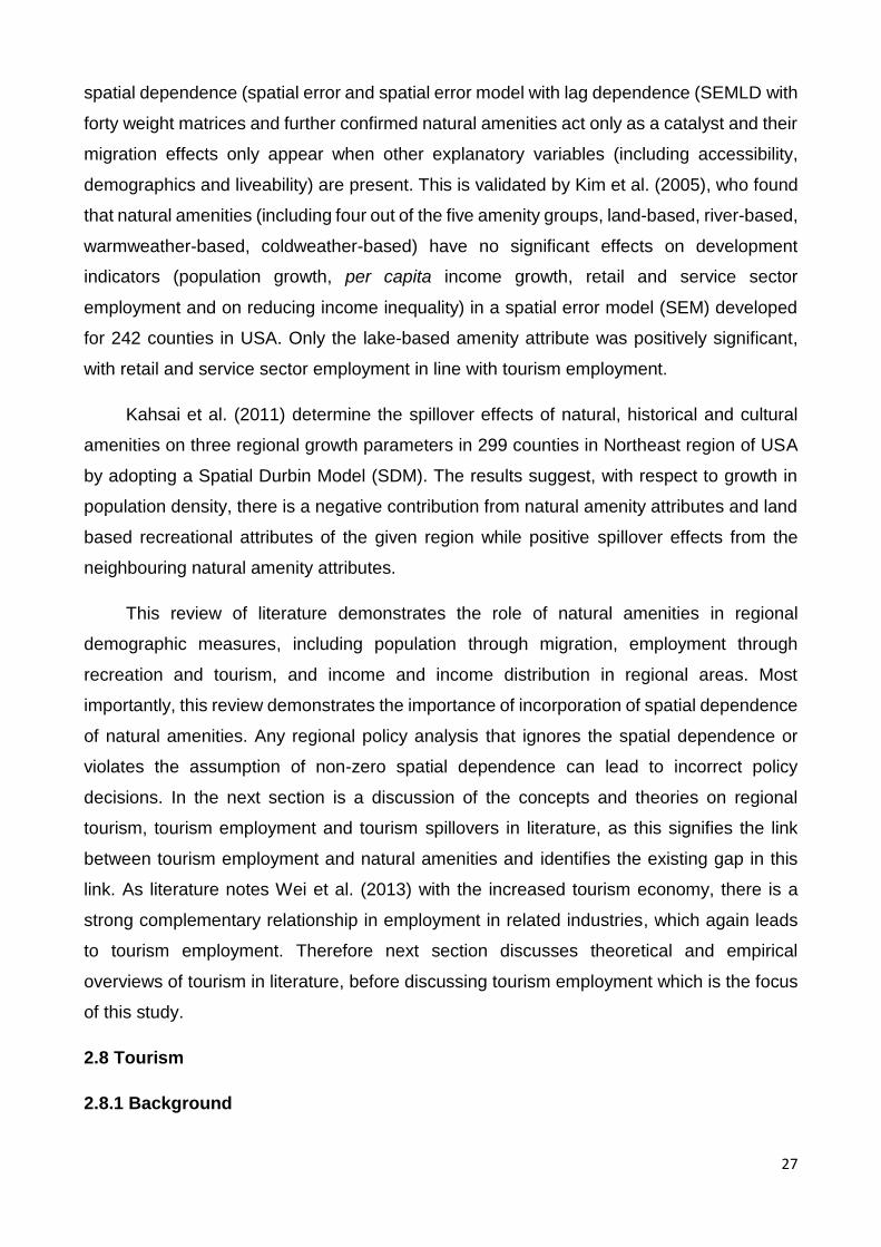
27

spatial dependence (spatial error and spatial error model with lag dependence (SEMLD with

forty weight matrices and further confirmed natural amenities act only as a catalyst and their

migration effects only appear when other explanatory variables (including accessibility,

demographics and liveability) are present. This is validated by Kim et al. (2005), who found

that natural amenities (including four out of the five amenity groups, land-based, river-based,

warmweather-based, coldweather-based) have no significant effects on development

indicators (population growth, per capita income growth, retail and service sector

employment and on reducing income inequality) in a spatial error model (SEM) developed

for 242 counties in USA. Only the lake-based amenity attribute was positively significant,

with retail and service sector employment in line with tourism employment.

Kahsai et al. (2011) determine the spillover effects of natural, historical and cultural

amenities on three regional growth parameters in 299 counties in Northeast region of USA

by adopting a Spatial Durbin Model (SDM). The results suggest, with respect to growth in

population density, there is a negative contribution from natural amenity attributes and land

based recreational attributes of the given region while positive spillover effects from the

neighbouring natural amenity attributes.

This review of literature demonstrates the role of natural amenities in regional

demographic measures, including population through migration, employment through

recreation and tourism, and income and income distribution in regional areas. Most

importantly, this review demonstrates the importance of incorporation of spatial dependence

of natural amenities. Any regional policy analysis that ignores the spatial dependence or

violates the assumption of non-zero spatial dependence can lead to incorrect policy

decisions. In the next section is a discussion of the concepts and theories on regional

tourism, tourism employment and tourism spillovers in literature, as this signifies the link

between tourism employment and natural amenities and identifies the existing gap in this

link. As literature notes Wei et al. (2013) with the increased tourism economy, there is a

strong complementary relationship in employment in related industries, which again leads

to tourism employment. Therefore next section discusses theoretical and empirical

overviews of tourism in literature, before discussing tourism employment which is the focus

of this study.

2.8 Tourism

2.8.1 Background

28

Tourism is a social, cultural and economic phenomenon that relates to the movement

of people to places from outside their usual place of residence (UNWTO, 2017). Tourism is

becoming one of the largest and fastest growing sectors in the world as one of the key

drivers to enhance the socio-economic standards of the community. It is a way to transform,

restructure and deliver sustainable economic development in declining regions (McLennan

et al., 2012; Zurick, 1992). Rural areas in the USA and around the world that depend on

tourism and recreation for employment can experience rapid economic growth and

contributes to the reduction of regional inequality (Deller et al., 2001; Green, 2001; Li et al.,

2016). A review of the literature indicates tourism, including , is an increasingly popular

strategy in regional economic development, due to its ability to enhance local job

opportunities and income with less training and infrastructure requirements (less demand

for skilled labour and technology) (Deller et al., 2001; Green, 2001; Lundmark and Müller,

2010).

2.8.2 Definitions and interpretations of tourism

It is noted in literature, with the maturation of the tourism industry, governments,

business organisations and researchers were started to define tourism with respect to

various perspectives and approaches (Leiper, 1979). As Jafari (2003) explains, tourism

means different things to different people. For governments, tourism means economic

benefits, employment, multiplier effects; for the industry sector it may be promotions,

arrivals, length of stay; for the host destinations, tourism means the type of tourist, inflation

and finally for the tourists it may be relaxation, indulgence and pleasure.

Therefore the interpretation of tourism has historically varied between disciplines and

this is reflected in the definition of the concept over time. According to Leiper 1979, the three

main approaches of defining tourism are: namely, “economic”, “technical” and “holistic”

identified between different disciplines(Leiper, 1979).

According to economic perspective, tourism has been interpreted as that which is a

nationally important industry and it involves wide range of activities, including provision of

transportation, accommodation, recreation, food and related services (ADTR, 1975) as in

(Leiper, 1979). This definition have been criticised due to it’s lack of human element and the

lack of spatial and temporal element.

In respect to the technical perspective, to define tourism, it is important to distinguish

between concept and the technical definition in 1968, the international Union of official travel

29

organisations (which is now known as the UNWTO) defined ‘visitor’ as any person visiting a

country other than that of his or her usual place of residence. This definition also covers two

forms of ‘visitors: the tourists’ who are defined as visitors who are staying at least twenty

four hours in the country for the purpose of journey that could be for leisure (recreation,

holiday, study, sports and religion) or for business, family , mission or meeting, or the

‘excursionists’ who are temporary visitors staying less than twenty fours in a visiting country,

which includes travellers and those on cruise ships. These various definitions of tourist

provide different concepts for a general definition for tourism framework (IUOTO, 1963) as

in (Leiper, 1979).

Finally, in the context of the holistic approach, tourism is identified as a ‘whole’ system.

Under the holistic approach several definitions are identified. Jafari (1977) defines tourism

as the study of people away from their usual place of residence, the industry that response

to their needs and the impacts that they and the industry have on the host’s socio cultural,

physical and economic environment.

Gunn (1972) identifies tourism as a closed system with five components:

people with the ability and desire to participate;

attractions for the participants;

services for the participants;

transportation for the movement of the participants to and from the attractions;

and

the information needed for the participation (Gunn, 1972) as in (Leiper, 1979).5

According to UNWTO, 2008 the concept of tourism is based on three criteria. The

geographical dimension, temporal dimension and the purpose. Tourism is the activity of

visitors, where a visitor is a traveller taking a trip to a main destination away from his/her

usual environment for less than a year, for any purpose (it could be business, leisure or any

family purpose) other than work. This has been further disaggregated based on temporal

dimension, where a visitor (domestic, inbound or outbound) is categorised as a tourist or

overnight visitor if the trip involves an overnight stay or as a same-day (excursionist) it is

otherwise.

Yu et al. (2012) defined the concept of tourism through examining by tourists’

perspective which relates to multiple dimension of several tourism definitions. Tourism is

5 More definitions of tourism under economic, technical and holistic context could be found in Leiper 1979

30

defined under several dimensions; usual environment, length of stay, purpose of the trip,

tourism characteristics and socioeconomic Covariates.

2.9 Theoretical perspectives of tourism

2.9.1 The framework of tourism as an open system: general system theory and

tourism

Leiper (1979) criticises definitions in the economic context due to the lack of human or

tourist elements , which is the focal point of tourism. Leiper (1979) notes by Gunn’s(1972)

holistic approach is more appropriate for expressing tourism as a framework in a more formal

system of theory setting, except for two points. First, Gunn (1972) fails to identify the

environmental interactions beyond the five elements of his organisation. Second, he

explicitly omits a clear definition of the tourism industry.

Leiper (1979) defines tourism as a formal system which recognises the

multidisciplinary approach of tourism. This defines tourism as a system involving

discretionary travel and the temporary stay of people away from their usual place of

residence for one or more nights, excluding tours made for primary purpose of remuneration.

This is an open system of five elements:

the human element which is the tourist;

three geographical elements; and

the tourist industry.

As shown in Figure 2.2, the elements of the system are the tourists, with three

geographical elements; the tourist generation regions, transit routes and the destination

regions. The fifth element is the tourist industry, which comprises all firms and organisations

involved in serving the specific needs of the tourist. There are spatial and functional

connections between these five elements and they interact and operate within social,

cultural, economic, technological and physical environments. This study employs Leiper

(1979) definition of tourism, which involves multiple aspects of tourism.

2.9.2 Jafari’s four platforms of tourism research

31

To understand tourism research and development, one of the most popular theories is

the four platforms/paradigms advocated by (Jafari (2001), 2003)), who suggests the

evolution of the tourism sector can be described in a sequential framework of four platforms:

1. advocacy;

2. cautionary;

3. adaptancy; and

4. knowledge based.

Figure 2.2: The tourism system Leiper (1979) from Meyer (2005)

Jafari (2003) addresses the change in attitudes in tourism research in an evolutionary

context, and argues the four platforms of tourism research developed sequentially over time.

Although each platform builds upon its predecessors, reaching a new platform does not

mean that preceding platforms disappear or become less significant as a whole (Jafari,

2001). Today, all four platforms co-exist in tourism in regional economies.

2.9.3 Advocacy Platform

Followers of the Advocacy Platform (1950-1960) consider tourism to be an ideal

activity, with less negative impacts on the host regions, and are mainly attracted to the

economic benefits of tourism. The advocates of this platform may be governments (public

sectors), private entities or any business related to tourism. The main focus is on tourism

providing myriad economic benefits. As it is a labour intensive industry with more

employment opportunities, and more multiplier effects, it is a viable option for economic

development and to gain foreign exchange.In line with (Jafari (2001), 2003)) advocacy

32

platform, the empirical evidence suggests tourism is commonly considered as a tool to boost

declining economies particularly with limited economic development opportunities through

employment generation and income (Deller et al., 2001; English et al., 2000; Green, 2001;

Hohl and Tisdell, 1995; Job and Paesler, 2013; Lundmark and Müller, 2010).

Further, as noted by Jafari (2003), the Advocacy Platform has been further

strengthened by pulling the non-market benefits of tourism into focus; these include tourism

preserves, and natural and man modified environments.

2.9.4 Cautionary Platform

The Advocacy Platform was replaced by the Cautionary Platform in the 1960s. This

newer platform emphasises the negative impacts or undesirable consequences of tourism

in economic, as well as non-economic perspectives. The negative attributes of tourism

employment, such as seasonality and low payments in jobs, generation of unskilled labour,

social and environmental pollution of the host communities, were taken into account by this

platform (Jafari, 2003).

2.9.5 Adaptancy Platform

The adaptancy platform appeared in the early 1980s and focussed on the forms of

tourism, which are more responsive to the host communities and their socio-cultural, man-

made and natural environments (Jafari, 2003). This platform is mainly concerned with the

impacts of tourism and is characterised by advocates of alternatives to mass tourism, such

as soft tourism, eco-tourism, responsible tourism and nature-based tourism, with minimum

negative impacts to the host community and to the environment. Further, this platform holds

these type of tourism are community-centred, not destructive, and both hosts and their

guests both will benefit (Jafari, 2003).

2.9.6 Knowledge-based Platform

Knowledge-based platform link with three previous platforms, but its main purpose is

to underpin a scientific body of knowledge on tourism, by considering tourism as a whole

system. This platform became evident in recent years and has deepened perceptions to

tourism. Tourism is a giant global industry, which generates benefits and costs, with

relationships between them. The advocacy and cautionary platforms focus on tourism

impacts and the adaptancy platform focuses on forms of development: these three platforms

cannot represent tourism as a whole. The knowledge-based platform considers tourism as

33

a whole and the resulting knowledge stimulates the development of theoretical concepts

and practical applications. Therefore, unlike other three platforms, this platform places itself

in a scientific foundation while maintaining its links with the others (Jafari, 2003).

2.10 This study in terms of Jafari’s four platforms

This study is consistent with Jafari’s platforms within the context of tourism literature

and research for four key reasons (see Figure 2.3). First, this study considers tourism as a

complementary income source for the regional communities with the downturn of mining in

regional Queensland, which is consistent with the Jafari’s advocacy platform. As noted in

the previous section, advocates of this platform observe the economic benefits provided by

tourism.

Second, this study uses perceived less positive attributes of tourism industry, such as

labour-intensive and low skill requirements, as an economic opportunity for the local host

communities. This research investigates cross-regional spillovers (that could be negative or

positive), which is consistent with Jafari’s cautionary platform.

Third, this study mainly focuses on nature-based tourism, which is an alternative to

mass tourism, and it is generally community-centred, and in which both hosts and guests

are benefit. This demonstrates the Jafari’s adaptancy platform.

Fourth, this study falls into the Jafari’s knowledge-based platform as contributes to the

scientific body of knowledge of tourism by investigating the geographical and non-

geographical spatial spillovers in tourism employment.

Tourism is a complementary

source of income to the

regional communities

Advocacy Platform

Negative impacts of tourism:

low skill, labour intensive

(opportunity for the regions),

cross regional spillovers

Cautionary Platform

Regions’ NBT

Adaptancy Platform

Knowledge –based Platform

Research on linking above all three Platforms – role of

natural amenities in tourism /geographical and non-

geographical spatial spillovers in tourism employment

34

Figure 2.3: Link between Jafari’s platforms and this research

2.11 Tourism in natural areas (nature-based tourism)

Both Smith (1994) and (D. Marcouiller, 1998) note the positive role of nature-based

public goods ( for example, parks and forests) as an input to the tourism production function.

Further they describe, similar to forest (natural resource) enter into the production function

of timber production, forest also enter into the production function of tourism production as

a non-market input. Marcouiller, D. (1998) notes the importance of nature-based tourism, it

is unlikely that people travel to forested regions because they have excellent restaurants or

uniquely wonderful hotel beds even though they may indeed exist!.

2.11.1 Nature Based Tourism (NBT)

NBT is considered one of the most popular regional development strategies across the

world due to its ability to create jobs with low demand for skill labour and infrastructure

(Margaryan and Fredman, 2016), and Australia is no exception. NBT is a type of tourism

that is more responsive to the host communities, to their socio cultural, man-made and

natural environments; hence it is consistent with Jafari’s Adaptancy platform.

There is no universally accepted definition of nature-based tourism. Lundmark and

Müller (2010) note NBT is more or less something to do with natural areas, but it could be

addressed from different perspectives. NBT has been defined in the literature from several

perspectives; namely, sociological perspectives, geographical perspectives and functional

perspectives. From the functional perspective (C. M. Hall and S. Boyd (2005)) define NBT

as focusing on three elements:

tourism in a natural setting (for example, adventure tourism);

tourism based on an element of the natural environment (for example, safari and

wildlife tourism, nature tourism and marine tourism); and

tourism etablished in order to protect natural areas, such as ecotourism and national

parks.

Further, Newsome et al. (2002) define NBT as tourism about the environment that is a

part of the tourism in natural areas. According to Newsome et al. (2002), tourism in natural

areas is categorised into three types:

35

tourism in the environment (adventure tourism);

tourism about the environment (NBT and wildlife tourism); and

tourism for the environment (ecotourism).

According to Tisdell and Wilson (2012) NBT is based on the visits to natural non-living

objects, or the utilasation of natural living objects or on a mixture of both. Natural non-living

objects includes moutains, canyons, lakes and waterfalls while natural living objects are the

wildlife.

Fredman and Sandell (2009)define NBT as “human activities occurring when visiting

nature areas outside the person’s ordinary neighbourhood” (p.24-25)which can be

considered a simplistic definition. As with Fredman and Tyrväinen (2010), Fredman et al.

(2009) define NBT as consisting of four recurrent components:

visitors to the nature area;

experiencing the nature area;

participating in an activity; and

the other related components such as local impacts and eco-tourism.

Weaver et al. (1999) define NBT as based on the extent to which the natural

environment is actually used as an attraction or setting. Valentine (1992) classifies activities,

based on the level of association, into three groups.

1. activities that depend on nature for attraction or the setting, such as wildlife

observation;

2. activities enhanced by nature, such as camping; and

3. activities, which are incidental in the natural setting, such as water skiing or rock

climbing.

Any tourism activity for which nature is beyond an incidental association is non-NBT,

which is the opposite end of the spectrum. Based on this association Weaver et al. (1999)

define NBT as the type of tourism that has a dependent, enhancive or incidental association

with the natural environment or some aspect, with respect to their utilised attractions and or

settings.

2.11.2 Working definition of NBT

Integrating the definitions of Lundmark and Müller (2010) , Fredman and Tyrväinen

(2010) and Weaver et al. (1999), for th puspose of this study NBT is defined as the tourism

36

that occurs in natural areas, outside the person’s neighbourhood and visiting a natural area,

associating with nature by enhancive or incidental and influencing the local community and

the region.

Based on a functional perspective, activities related to nature such as ecotourism,

wilderness tourism and adventure tourism also will be included (Hall, 2009). The definition

also includes man-modified natural areas, such as parks in regional areas, as commodities

of nature-based tourism.

2.11.3. Experiences of natural amenities in NBT

Natural amenities exist in many different forms and their contribution on experiences

may vary across different forms. It is evident in literature that the tourist experience in nature-

based tourism varies from adventure to escape. (Amuquandoh et al., 2011; Mehmetoglu,

2006) (see Figure 2.4)

Figure 2.4: Experiences of NBT

2.12 A Conceptual framework of nature-based tourism and regional economies

Nature-based tourism is not only about the tourism industry and the number of visitors

to the regional areas (Fredman and Tyrväinen, 2010). It is an interactive system with

Experiences of NBT

To engage in challenging

physical activity

(Adventure)

To engage in non-

challenging physical

activity - walking

Social – to be friends

and relatives

Education/knowledge

Escape

Relaxation

Being close to

nature

Scenic beauty

37

backward and forward linkages between different agents and entities. The conceptual

framework of regional tourism, with particular focus on nature-based tourism, integrates

multifunctional regional landscapes, the regional nature of natural amenities and their links

in regional development. The conceptual framework consists of several elements.

The tourism product is unique compared with other products, due to its complexity.

The supply of regional tourism products involves complex combination of factors and

attributes. First, is the importance of natural resources, as latent non-market inputs that are

unpriced public goods, which represents the supply side of the system. The value of these

natural amenity endowments is integral in rural tourism production. Nature-based tourist

destinations, such as parks, rivers and mountains, are the main pulling factors and they are

central to nature-based tourism.

The supporting services and access infrastructure, such as accommodation, visitor

centres, parking, trails, guides and local public transportation, also contribute to the rural

tourism supply. In this manner, the local community is highly integrated into the system from

the supply perspective, which includes, rural recreational services such as rural parks,

farmers’ markets, arts and crafts, local public transportation and parking. These attributes

are tied with other actors involved in supply of opportunities and their links to alternative land

use (Dissart and Marcouiller, 2012; Fredman and Tyrväinen, 2010).

The second component of the model are the indirect and joint producers of the rural

tourism product. This includes joint producers of multifunctional landscapes, particularly

consumptive-use or consumptive (logging) when produced jointly with a non-consumptive

produce (amenity)6. As Dissart and Marcouiller (2012), explain (and as described by

Clawson and Knetsch (1966), from a recreational perspective, the natural resource becomes

a recreation product or tourism product as a combination of natural qualities and

experiences with the ability and the desire of people to use it.

Therefore, in rural tourism, natural amenities are considered the latent non-market

input to the rural tourism product, which is jointly produced by various private and public

entities, such as rural amusements, recreational equipment providers, tourist guides,

instructors and also rural specific markets This also includes landholders, government

organisations and environmental conservation institutions.

6 There is a trade-off between consumptive and non-consumptive use, which will not be discussed in this literature review as it is

beyond the scope of this study). This includes other competing resource users, such as agriculture, forestry and mining.

38

Third, the demand side involves nature tourists who are the visitors of the natural area,

and who participate various forms of activities such as, bush walking and hiking, boating

and recreational fishing and consumers at local markets.

This demonstrates nature-based tourism is attributed by many stakeholders; mainly

the local community and other stakeholders involved in management, utilisation and

protection of natural resources. This further signifies the importance of NBT in regional

economies in the study area (see Figure 2.5).

Figure 2.5: The Conceptual framework of system of regional nature based tourism

After (Dissart and Marcouiller, 2012; English et al., 2000; Lundmark and Müller, 2010)

Rural nature-based tourism,

with respect to NBT

Other suppliers link to NBT:

rural parks

recreational services

arts and crafts markets

farmers’ markets

service and

infrastructure:

parking, transportation

Joint Producers of

multifunctional landscape:

The trade-off between:

consumptive and non-

consumptive users,

agriculture producers,

miners,

infrastructure

producers,

tangible governance –

the government, and

intangible governance –

the local community

and

the social capital

Demand for NBT

Nature tourists or visitors to

the natural areas and

participants in various

activities; such as hiking,

boating and bushwalking

Supply of NBT: Natural

amenity endowments, parks,

rivers, mountains

39

2.13 Approaches to measuring tourism activity

Tourism is not well defined as an industry and is considered an export sector in regional

economies (English et al., 2000). Given the multi-attributable activities involved in tourism,

tourism performance can be measured using several different perspectives. Measuring

tourism through the demand side perspective is the process of measuring trends, forecasts

and travellers’ perceptions. With respect to the supply side perspective, it is the economic

scale and the impact of tourism.

Most tourism impact studies are based on tourism expenditure and employment

associated with visitor demand. Measuring the expenditure or employment associated with

visitor demands is done by surveys, investigating input-output techniques to estimate

spending through visitors and by estimating tourism employment through secondary data

sources (English et al., 2000; Leatherman and Marcouiller, 1996).

2.13.1 Tourism employment

Wei et al. (2013) note that the tourism economy positively correlates with tourism

employment in China in three ways. Firstly, the technology level, which is associated with

tourism economy, and leads to more employment opportunities. Secondly, with the

increased tourism economy, there is a strong complementary relationship in employment in

related industries, which again leads to tourism employment. The third way is referred as

‘environmental pressure’, which increases tourist arrivals and also leads to increased

tourism employment.

It is well known in literature, that tourism is considered an industry that has the ability

absorb surplus labour; one of the main elements in tourism development is supply of labour

(Falk and Broner, 1980; Szivas et al., 2003). As a consequence of any change in an

economic system, there is a change in human capital; the tourism industry serves as a

‘refuge’ to find a job in difficult times. Tourism is understood to be an accessible and

attractive option during times of economic transition and labour displacement (Szivas and

Riley, 1999; Szivas et al., 2003).

Szivas and Riley (1999) noted that during the time of economic transition, such as from

communism to capitalism or extractive to non-extractive industries, the tourism industry is

an expanding industry with low human capital that will provide refuge for labour. Szivas and

Riley (1999) further note that at a time when the workforce is devalued and redundant, it

40

moves to industries with higher growth potential that also require lower skills. The particular

universal attributes of the industry, such as”

the “non-factory” nature of work (Riley, 1986),

less distinction between leisure time and work (Urry, 1990),

more interpersonal contacts and flexibility,

higher proportion of unskilled labour, seasonality, and

high intra-industry mobility,

These provide a competitive advantage for this industry over others (Szivas et al.,

2003). Tourism is an accommodating industry that requires a wide range of jobs with a

variety of human capital requirements. Therefore, job seekers find tourism employment is

more attractive, as it provides a wide range of choices in skill requirements, working

conditions and even in payment. However, it is noted despite the advantages in tourism

employment, matching the human capital with the job is the most attractive attribute in

tourism employment (Szivas et al., 2003).

Szivas et al. (2003), further argue labour mobility into tourism is beneficial for the

economy, if the labour is more productive in tourism than it was in the previous employment.

It is an economic disadvantage if labour moves into tourism, when it is employed and needed

by other sectors in the economy. This creates labour shortages and the displacement of

other industries by tourism. However, this is not the case with respect to this study, as this

study considers tourism employment as a complementary to other sectors, and labour

mobility between sectors is beyond the scope of this research.

Szivas and Riley (1999) study investigates the pattern of labour mobility to tourism

(after collapse of communism), the impact of the mobility and the motives of the mobility, in

a random sample of 351 direct tourism workers in Hungary (including Budapest). The study

found there as a broad spectrum of industries from which workers migrated (trade and

manufacturing topped the list) while there was no migration from the mining industry.

Further, it notes that in addition to inter-industry migration there was migration with respect

to geographic context. Regardless of the motive for mobility, the impact of mobility was

generally positive with respect to several attributes, including job security, income, social

status and career prospects. The results also show the most important motive to move to

tourism was refuge, followed by other positive impacts.

41

Despite the popularity of tourism as a major driver in regional economies, economic

development through tourism has advantages and disadvantages. In line with Jafari’s

advocacy and cautionary platforms, the literature suggests rural areas that depend on

tourism and recreation for employment have experienced rapid economic growth, but that

most of this employment is low-skilled, low paying and only seasonal (Deller et al., 2001;

Green, 2001; Jafari, 2001, 2003).

Therefore, while acknowledging that tourism employment is low paying and seasonal,

this study uses tourism employment as the proxy for tourism performance in regional

economies.

2.13.2 Measuring tourism employment

Although the tourism industry is an important contributor to the overall economy in a

country, the Systems of National Accounts (SNA) does not consider tourism as a single

homogenous industry, due to its multiple provisions of products and services (Chhetri, 2014;

Pham and Marshall, 2012). Therefore, to measure the economic significance of tourism

industry, Tourism Satellite Accounts (TSA) is supplementing SNA. TSA was produced in

2000. The Tourism Division of Asia-Pacific Economic Cooperation (APEC) and the World

Travel and Tourism Council (WTTC) published “ The Economic Impact of Travel and

Tourism Development in the APEC Region 2000” (WTTC, 2000). Based on this report, TSA

notes tourism employment as comprising four parts:

The first is direct tourism employment, where services are directly provided to

tourists; this includes accommodation, restaurants, airline and other transport.

The second is indirect tourism employment, which provides jobs supporting the

tourism industry, such as airline food suppliers and wholesalers.

The third is direct employment through the tourism suppliers industries, such as

tourism souvenir producers.

The fourth is indirect employment to tourism suppliers industries.

With respect to Australian context, TRA prepares TSA, including state TSA. The

National and state TSA measure both direct and indirect contribution of tourism to national

and state economies. The direct contribution is measured based on TSA framework, while

indirect contribution is measured through using input-output (IO) modelling techniques. The

direct contribution refers to any transaction between visitors and producers of goods and

42

services, which involves direct physical or economic connection such as suppliers and

services to the visitors in hotel accommodation.

Indirect effects refer to flow-on effects created by the inputs for the supplying goods

and services to the tourists such as fresh food suppliers and the electricity used. Although

TRA estimates the national and state TSA, investigating tourism employment in more

disaggregated levels (such as county levels in USA) in Australia it is limited to tourism

regional7 levels in tourism literature.

(English et al. (2000); Gunderson and Ng (2005)) note one of the major issues in

estimating tourism employment in local economies is the fact that many of the businesses

that cater tourists also cater to local residents and visitors on trips other than recreation

(such as visiting families, friends or business trips). In an attempt to disintegrate the

recreation (amenity ) based travel from local and non-tourism (business and visiting family

and relatives) based travel, (English et al., 2000; Gunderson and Ng, 2005) treat non-

tourism based activities as a function of population and recreational based travel as a

function of recreation endowments of the counties. A regression model with population and

recreational tourism of a county is used to separate employment created by recreation-

based travel by non-recreational based travel. However, by this method, the minimum

requirement technique considers one region within the cluster as the region with local

demand employment only (that caters for local residents only) and zero tourism-related

employment, which is a restrictive assumption.

To differentiate the export employment (English et al. (2000); Gunderson and Ng

(2005)), which is the employment created by recreational and non-recreational based

visitors, the minimum requirement technique is used. The counties (in US) are clustered on

some common attributes, based on population density, proximity to the metropolitan area,

forest cover, pasture cover and cropland cover. Within each cluster, the county with the

minimum employment percentage of each tourism related sector was assumed to be the

county with no export employment. In all other counties within the cluster, the excess to the

minimum requirement is assumed to be export employment percentage.

Chhetri et al. (2008) and Chhetri (2014) use the ABS Census data on Basic Community

Profile and Journey to Work (JTW) to estimate the tourism-related employment in Statistical

Local Areas (SLAs) in South East Queensland. Based on Australian and New Zealand

7 According to ABS (date?), tourism regions are classified based on a structure not defined and maintained by ABS. ABS defines

tourism regions as a collection of Statistical Area Level 2s (SA2). This is in detail in Chapter 3

43

Standard Industrial Classification (ANZSIC), codes were given to industries in JTW and used

to identify the tourism sector employment. To identify the tourism related employment, the

industry sector ‘Accommodation, Cafes, Restaurants’ and other sub-sectors (Casinos-

9322, Mueums-9220, Recreational parks and Gardens- 9239 based on four-digit codes) are

used as the surrogate measure for tourism related employment. Although this method of

estimation is appropriate to estimate the direct employment in Tourism and Hospitality (T&H)

sector, this method cannot be used to estimate the indirect employment or employment from

flow on effects in tourism.

Wei et al. (2013) estimate the relationships between tourism economy and tourism

employment. In this study, tourism employment was measured based on the method

adopted by Annual Tourism Statistics system of the China National Tourism Administration

(CNTA). Although there are a large number of studies, which discuss the general

employment models, studies specifically on measuring tourism employment are very limited

in literature.

Based on the limited existing literature on measuring tourism employment, there is no

unique method by which to measure tourism employment at a regional level. As this study

measures direct and indirect regional tourism employment the method adopted by this study

is based on national and state TSAs. This is discussed in detail in Chapter 4.

2.14 Summary

Natural resources play a critical role in regional economies, but have been transformed

from market to non-market commodities in rural economies. It is evident there is a shift from

traditional good production (extracting industries such as mining, agriculture and

manufacturing) to more service oriented industries, such as tourism and retirement-oriented

services. Hence natural amenities play a critical role in regional economies.

Natural amenities contribute to regional economies in many ways. Natural amenities

influence the regional economies through population (in-migration), employment including

tourism employment, per capita income and also income inequality (Deller et al., 2001;

English et al., 2000; Henderson and McDaniel, 2005; McGranahan, 1999). Further, natural

amenities are not randomly located and are usually spatially clustered. Recent studies show

there is a spatial dependence of natural amenity attributes on regional growth measures,

including tourism.

44

This literature review discusses the theoretical foundation of tourism research and it

demonstrates how this study is supported by Jafari’s platform of tourism research. Tourism

is considered an industry that has the ability to absorb surplus labour and one of the main

elements in tourism development is the supply of labour. The tourism industry serves as a

‘refuge’ to find a job in difficult times.

There is an identified aim to combine the role of natural amenities in tourism

employment and the ability of the tourism industry to absorb excess labour during

economically difficult periods. Hence, the review of literature indicates tourism, particularly

nature-based tourism (NBT), is an increasingly popular strategy in regional economic

development and natural amenities plays significant role in regional tourism.

Although the tourism industry is an important contributor to the overall economy in a

country, the Systems of National Accounts (SNA) does not consider tourism a single

homogenous industry, due to its multiple provisions of products and services. There is only

very limited literature on measuring tourism employment at regional or local levels. The

National and state TSAs measure both direct and indirect contribution of tourism to national

and state economies.

In Chapter 3, an overview of tourism in Queensland, one of the fastest growing

tourism regions in Australia is provided.

45

Chapter 3

An overview of tourism in Queensland

With the resources boom now behind us, tourism has the potential to be Australia’s fastest

growing industry.

State Tourism Satellite Accounts 2014-15 (TRA, 2016a) p.2

3.1 Introduction

Despite the recent downturn in the Australian resource sector, the tourism industry

remains resilient and is one of the largest and fastest growing sectors in Australia. The

tourism industry will play a critical role as one of the growth engines in the Australian

economy. Tourism Gross Domestic Product (GDP) reached 7.4 per cent in 2015-16, well

ahead of the rest of the economy (TRA, 2017b) The tourism industry has been recognised

as one of the five super-growth sectors that will drive the Australian economy over the next

decade. (TRA, 2015).

Tourism is a major export earner for Australian economy, a major source of

employment and a key driver in the national economy. Compared with other industries, the

benefits of tourism are widely spread and not geographically concentrated; almost half of all

expenditure in tourism is benefitted by regional Australia (TRA, 2017a) .

Australia has a competitive advantage in tourism in comparison with other countries

due to several reasons. It is close to growing Asian markets, it has a richness of natural

amenity, a safe environment and the depreciation of the Australian dollar favours Australian

tourism too (TRA, 2015). As noted, Australia is geographically strategically placed to

harness the benefits of an expected five-fold growth in the Asian middle class population

over the next twenty years.

There were 8.35 million visitor arrivals during the annual period that ended in February

2017, which is an increase of 10.1 per cent or 736,000 extra visitors, relative to the previous

year. Most importantly, leisure arrivals (holiday and visiting friends and families) was the

highest among international arrivals an increase of 11.7 per cent since last year, which

further demonstrates the rising trend of this industry in Australia. (Tourism, 2017). Tourism

Research Australia forecasts that in 2024-25, there will be an increase of 48 per cent

international visitors, compared with 2016-17.

46

The next section of this chapter begins with a discussion of the economic significance

of tourism in Australia, followed by the economic contribution of tourism to Queensland.

Then it briefly reviews the existing national and state level tourism strategies and tourism

forecasts for the future. This is followed by a description of the tourism workforce in

Queensland, which provides an insight into the main sectors of tourism employment. Then

it discusses the twelve8 identified tourism destination regions in Queensland. This section

provides a detailed description of the tourism destination regions, including the economic

contribution of the tourism sector, based on tourism employment, Gross Regional Product

(GRP) and Gross State Product (GSP). This section also provides a brief overview of the

geography of the region and a list of LGAs that encompasses in each tourism destination

region. A discussion of the main natural amenities that attract tourists to Queensland will be

followed by the conclusion of the chapter.

3.2 The economic significance of tourism

In 2015-16 the tourism industry created 580,200 direct jobs, equivalent to 4.9 per cent

of Australia’s total workforce. This figure is larger than that of mining (227,800 workers),

agriculture (321,600 workers) and utilities services (144,000 workers). In addition to direct

employment, the total flow-on share in national employment (direct and indirect ) increased

up to 7.9 per cent of total Australian workforce, or 934,300 workers. This is an increase of

28,200 from 2014-15, or 906,100 workers. The increase of 7.9 per cent share of national

employment is 0.1% point higher than the previous year, and above the long-term average

share of 7.6 per cent since 2006-07.

New South Wales, Victoria and Queensland contributed around three quarters of total

tourism employment (direct and indirect). Unlike other industries, the tourism industry spread

across most of the sectors in Australian economy, including retail, food and accommodation,

transport and recreation. The industries that contribute directly to direct tourism employment

are food services, retail trade, accommodation, education and training.

The food industry sector is the main employer of tourism workers, which includes cafes,

takeaways, tavern and bars. This industry sector employed 194,300 workers in 2015-16; an

increase of 5300 workers compared with 2014-15.(STSA, 2017)

8 The number of tourism destination regions is reported as twelve or thirteen as Bundaberg and Central Queensland is noted as on tourism regions Southern Great Barrier Reef in some occasions (TEQ, 2015-16)

47

In same period, the Gross Domestic Product (GDP) from tourism increased 7.4 per

cent ($3.7 billion) in nominal terms, which accounted for $53 billion. This is well ahead of

the rest of the economy (as shown in figure 3.1). This was equivalent to 3.2 per cent share

of total GDP, which is the highest share since 2003-2004. In 2015-2016 GVA (Gross Value

Added) increased 7.5 per cent or $3.4 billion, which represented 3.1 per cent of the national

economy. This is more than that of agriculture, forestry and fishing (2.6 per cent share of

national economy) (TRA, 2017a). The sectors that contributed most to the growth in GVA

are food services (up 9.5% to $9.0 billion), air and water transport (up 9.4 per cent to $8.2

billion) and accommodation (up 7.1 per cent to $7.5 billion).

Tourism also contributes to the Australian economy by reducing trade deficit. In 2015-

16, through aggregate expenditure by international tourists, Australian export earning was

$34.2 billion, which is an increase of $3.4 billion on 2014-15. This makes tourism one of the

largest export service sectors in the Australian economy, accounting for 11 per cent share

of Australian exports of the year. The tourism imports (the expenditure by Australians

travelling overseas) was $38.6 billion in 2015-16. Most importantly, over this period export

earnings increased faster than imports, which resulted in a decline in trade deficit. Compared

with $5.2 billion in 2014-15, in 2015-16 Australia’s tourism trade deficit narrowed to $4.3

billion, a decrease of 15.9 per cent. (TRA, 2016b).

In 2015-16, tourism consumption was $130 billion, an increase of 6.1 per cent

compared with 2014-15. Out of total tourism consumption, domestic tourists contributed 74

per cent, while international tourists contributed 26 per cent. Accommodation, eating out,

long distance transport and shopping were the main items that accounted for tourism

expenditure. In 2014-15, New South Wales, Victoria and Queensland contributed more than

three quarters of the total Australian domestic tourism consumption, 31 per cent, 23 per cent

and 23 per cent respectively.

3.3 Tourism 2020 Strategy and Forecasts

Although, the Australian tourism industry is strengthened by many positive forecasts,

it also faces many challenges. The global tourism market is highly competitive; over 190

tourism organisations compete for international visitors. The industry is highly susceptible to

international events, economic uncertainties, the risks of travelling, and economic and

political instability (local and global).

48

Figure 3.1: The growth of the tourism economy compared to the Australian economy

during the period of 2000-01 to 2015-16.

Source Tourism Research Australia (TRA, 2017a)

Therefore, in order to ensure the Australia’s ongoing high position in global tourism, to

remain as an attractive destination for international tourists and to maintain the growth in

tourism infrastructure, attractions and training, the Australian Government and the tourism

industry implemented Tourism-2020 Strategy. Tourism 2020, the National Strategy for

tourism, aims to double the overnight spend to between $115 and $140 billion by 2020. In

order to achieve this target, , there is a reform to integrate national and state tourism plans

into regional development and local government planning.

Tourism forecasts for 2017 show that by the end of 2020, the forecast total

spend(excluding day trips) will reach $ 131 billion, only slightly above the target set under

the Tourism 2020 strategy. Of international and domestic visitors, the former capture the

greater share of tourism spending, and it is expected there will be a 10 per cent increase

from 2016-17 to 2026-27, while domestic tourism spending continues with moderate growth.

In terms of international tourists, China will be the largest target with respect to inbound

arrivals and inbound spending, overtaking New Zealand. Over the next two years,

international visitor number is expected increase by 13.1 per cent from 2016-17 to 2018-19.

Asia will dominate the overseas market, contributing 64 per cent of all visitor growth between

these two time periods, led by China, and followed by India and Japan.

49

Domestic tourist growth is expected to be moderate over the same period, as a result

of historically below average Australian economic growth and a stagnated wage rate. It is

expected the 2018 Commonwealth Games on the Gold Coast, will boost domestic and

international travel (TRA, 2017b).

3.4 Queensland tourism and the Queensland economy

Queensland is commonly known as the ‘Sunshine State’ in Australia and it is popular

with tourists due to its pristine sandy beaches, tranquil forests, amusement parks, heritage

sites and the ‘Outback’. One in five Australians lives in Queensland. It had the population of

4,703,193 people according to ABS Census 2016 (ABS, 2017a). Queensland is the second

largest state (in square kilometres) in Australia and it is third most populous state, after

Victoria and New South Wales. Queensland has the highest Aboriginal and Torres Strait

Islander population of 4.0 per cent, compared with the national percentage, of 2.8 per cent

(Treasury 2017) .

Queensland has a modern, diversified economy strengthened by mainly agriculture,

resources, construction, tourism, manufacturing and services. Queensland’s economic

growth has been above the national average, between 2015 and 2017. The agriculture

sector in Queensland is the original platform of the Queensland economy, accounts for 2.5

per cent of the state’s economy and provides 57,000 jobs to the Queenslanders (contributing

2.4 per cent share to the Queensland employment). Queensland’s resource sector has been

the key driver of the state economy, while Queensland’s coal and bauxite reserves are

largest in the world. In 2014-15, this sector contributed 7.4 per cent to the state economy

and 1.9 per cent to state employment, which is a decline of 10.6 per cent compared with the

previous year. With respect to tourism in Queensland, in 2014-15 tourism in Queensland

was the second largest tourism market in Australia, next to New South Wales, with 24.9 per

cent of national tourism and employing 130,900 people in the sector (Treasury 2017).

This study selected Queensland as a good location for an empirical study to explore

the spatial patterns of tourism employment spillovers and natural amenities, due to its

richness in natural amenities and significance of its improving tourism sector and effect on

the state economy. With the expansion of the tourism sector, with a 9.5 per cent share of

total employment in Queensland, demonstrates the economic significance of the tourism

sector in the future and validates the importance of exploring tourism employment spillovers

in the state, for effective future planning and decision-making in this sector.

50

Moreover, the selection of Queensland as the study area was driven by several factors,

including the public policy strategy in Queensland that focuses on tourism as one of the

main strategies of economic development in Queensland. Tourism has been identified as

the one of the four pillars that contributes to a strong, future Queensland economy by the

Queensland Government state Planning Policy 2014. The three other pillars are agriculture,

resources and construction.

3.4.1 Economic significance of the Queensland tourism industry

The tourism industry in Queensland is vibrant, with a rapid and noticeable growth in

2015-16, where domestic tourists contributed more than $23.0 billion worth of goods and

services in the state, which is $1635 million more than the previous year 2014-15.

The tourism sector plays a critical role in Queensland’s economy. In 2015-16 tourism

directly contributed 138,000 jobs (that is, 5.8 per cent) jobs and indirectly 88,000 jobs to the

Queensland economy. That is 9.5 per cent overall of employment to the total state

employment, which is substantially more than the mining (2.5 per cent) and construction

(8.8%) industries. Queensland is the second highest contributor to national tourism

employment, followed by New South Wales, which has a 24 per cent share of direct tourism

and 25 per cent share of indirect tourism. The tourism-related industries that contributed

most to total tourism employment were food, retail, accommodation and education and

training.

In the 2015-16 financial year the tourism industry directly contributed $12.6 billion to

the Queensland economy, accounting for 4.0 per cent of Queensland Gross State Product

(GSP). As tourism is an industry with strong links with other sectors of the economy, the

indirect contribution to the state’s economy was $12.4 billion. In 2015-16, the tourism

industry was worth $25 billion or 7.9 per cent of total GSP to the Queensland economy,

including both direct and indirect contribution. The indirect or flow-on contribution of tourism

in Queensland is for every dollar that is spent in the tourism industry, an extra 84 cents spent

elsewhere in the economy .The share of GVA by tourism to the total state GVA is the second

highest contribution across all states, contributing $10.2 billion and $10.0 billion directly and

indirectly, which demonstrates the significance of the industry to the state and national level

(TRA, 2016b)

Most importantly, domestic visitors play a significant role in tourism in Queensland.

Unlike the national context, with respect to tourist visitations, domestic tourists shows the

51

largest contribution, accounting more than two thirds of total nights spent by tourists in

Queensland. Brisbane is the most popular destination, followed by the Gold Coast, Tropical

North Queensland and the Sunshine Coast.

3.5 Tourism Workforce

Although the tourism industry is an major contributor to the economy, it is not

considered a single industry due to its diverse goods and services, and thus it is not included

in System of National Accounts (SNA) (Pham and Marshall, 2012). There is no specific

identifier in ANZSIC for the tourism industry. As shown in Figure 3.1, the industry consists

of multiple sectors, as visitors consume goods and services across wide range of sectors in

the economy. The industry includes transport, accommodation, attractions, events, food

services, clubs and casinos, retail, arts and recreation, travel agencies and tour operators,

education and training.

Although there is a wide range of jobs within the tourism industry, there are eleven

occupations that represent the majority of the workforce in the industry, including

accommodation and hospitality managers, housekeepers and cleaners, fast food cooks and

kitchen hands, receptionists, waiters, bar attendants and baristas, chefs, cooks, cafe

workers, travel and tourism advisors and air transport professionals. Most importantly two

thirds of direct employment in tourism is outside the capital city Brisbane region, which

highlights the importance of the tourism industry to the state’s remote and rural regions.

Table 3.1 shows café, restaurants and takeaway food services dominate direct tourism

employment, which is 26 per cent of the total direct employment, followed by retail trade and

accommodation, which are 17 per cent and 15 per cent of the direct tourism employment

respectively.

The next section discusses regional tourism in thirteen tourism destination regions in

Queensland and the economic significance of the tourism sector to each tourism destination

region, and to Queensland, in general.

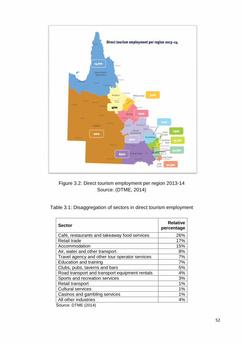
52

Figure 3.2: Direct tourism employment per region 2013-14

Source: (DTME, 2014)

Table 3.1: Disaggregation of sectors in direct tourism employment

Sector Relative

percentage

Café, restaurants and takeaway food services 26%

Retail trade 17%

Accommodation 15%

Air, water and other transport 8%

Travel agency and other tour operator services 7%

Education and training 7%

Clubs, pubs, taverns and bars 5%

Road transport and transport equipment rentals 4%

Sports and recreation services 3%

Retail transport 1%

Cultural services 1%

Casinos and gambling services 1%

All other industries 4%

Source: DTME (2014)

53

3.6 Regional tourism

Regional tourism includes tourism in concentrated tourism areas such as coastal

areas, urban areas and also the countryside, hinterlands and coastal areas outside, the

main capital cities. It is not a particular activity or the experience scape; but it is the specific

attributes of the place to which tourists are attracted. It includes a wide range of tourism;

namely, , eco-tourism, cultural tourism, food and wine tourism, backpacker tourism and

adventure tourism (Prosser, 2000).

Regional and rural economies in Australia, and their communities, are continuing to

encounter various challenges and pressures as a result of the social and economic changes

occurring across industrialised countries globally . The main drivers for this pressure

including more efficient and less labour intensive technology in agriculture practises, trade

liberalisation, rising conflicts between competing land uses, increasing unemployment,

change in population patterns and an increased awareness of the environment and, most

importantly, the decline in traditional industries including the mining sector.

As a result of this changing nature of regional economies, the tourism industry is

becoming a major industry in regional areas. Although, international tourists contribute to

strong growth in Australian tourism, domestic tourism still plays a major role in tourism in

Australia and most of the domestic visitor nights are spent outside major capital cities. More

than 60 per cent of the international and domestic visitor nights in Australia are spent outside

the main capital cities. Further, there is greater market for natural and cultural attractions

with ‘authentic’ experiences for both domestic and international tourists and Australian

regions are well placed to cater for these markets., further highlights the importance of

regional tourism to Australia (Prosser, 2000).

3.6.1 Queensland tourism destination regions

Based on the tourist attractions and the characteristics and the economic contribution,

Tourism Research Australia divides Queensland into twelve tourism destination regions9 as

shown in Figure 3.2. According to ABS (2017b), tourism regions are classified based on a

structure not defined or maintained by the ABS. ABS defines tourism regions as a collection

of Statistical Area Level 2s (SA2). These regions are divided based on the tourism attributes

and the economic contribution of the tourism industry of each region (Pham et al., 2010).

The LGA boundaries do not exactly fit with the tourism region boundaries, as these regions

9 The terms ‘tourism destination regions’ and ‘tourism regions’ are used interchangeably in this thesis

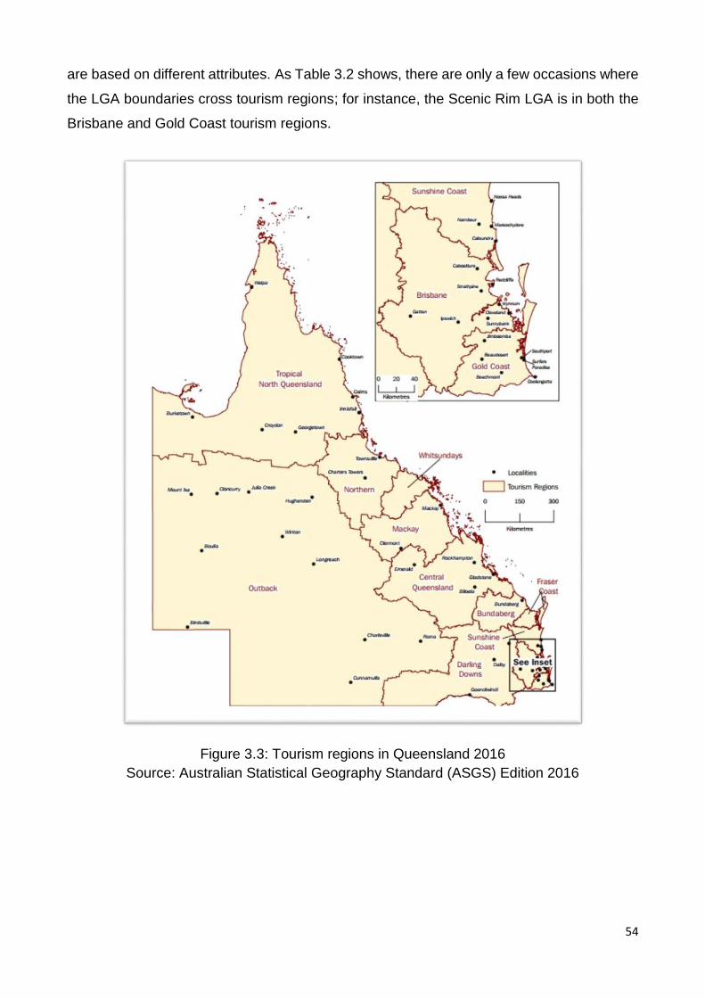
54

are based on different attributes. As Table 3.2 shows, there are only a few occasions where

the LGA boundaries cross tourism regions; for instance, the Scenic Rim LGA is in both the

Brisbane and Gold Coast tourism regions.

Figure 3.3: Tourism regions in Queensland 2016

Source: Australian Statistical Geography Standard (ASGS) Edition 2016

55

Table 3.2: Tourism destination regions and LGAs in each tourism destination region.

Tourism Region LGAs

Whitsundays Whitsundays

Tropical North Queensland

Aurukun, Burke, Cairns, Carpentaria, Cassowary Coast, Cook, Croydon, Doomadgee, Douglas10*, Etheridge, Hope Vale, Kowanyama, Lockhart River, Mapoon, Mareeba*, Mornington, Mount Isa, Northern Peninsula Area, Pormpuraaw, Tablelands, Torres, Torres Strait Island, Weipa, Wujal Wujal

Brisbane Brisbane, Ipswich, Lockyer Valley, Logan, Moreton Bay, Redland, Scenic Rim, Somerset, Sunshine Coast

Bundaberg Bundaberg, North Burnett

Central Queensland Banana, Central Highlands, Gladstone, Livingstone*, Rockhampton, Woorabinda

Southern Queensland Country (Darling Downs)

Balonne, Cherbourg, Goondiwindi, Maranoa, South Burnett, Southern Downs, Toowoomba, Western Downs

Fraser Coast Fraser Coast

Gold Coast Gold Coast, Logan, Scenic Rim

Mackay Isaac, Mackay,

Northern (Townsville) Burdekin, Charters Towers, Flinders, Hinchinbrook, Palm Island, Townsville

Outback

Barcaldine, Barcoo, Blackall-Tambo, Boulia, Bulloo, Cloncurry, Diamantina, Flinders, Longreach, McKinlay, Mount Isa, Murweh, Paroo, Quilpie, Richmond, Winton

Sunshine Coast Gympie, Noosa*, Sunshine Coast

Source: Tourism Research Australia

3.7 The regional economic contribution of tourism in Queensland

The regions can be divided into three broad categories:

1. Main tourism destinations which includes Gold Coast, Tropical North Queensland and

Whitsundays

2. Regions with strong links as indirect input suppliers but not necessarily tourism

focused; which includes Darling Downs (suppliers of agricultural inputs to the tourism

industry)

3. Regions with both direct and indirect tourism links; which includes Brisbane region

(Deloitte, 2017b).

Each tourism region is discussed separately below.

10 * These four LGAs are Queensland de-amalgamated councils in 2013. Hence, they were not considered as separate LGAs in this study.

56

3.7.1 Tropical North Queensland (TNQ)

The Tropical North Queensland TNQ region is a large area, with twenty-six LGAs

extending from Mission Beach in the south, to Cape York and the Torres Strait in the north,

and Gulf Savannah in the west. This region boasts its natural tourist attractions; out of five

World Heritage areas in Queensland, TNQ has two, the Great Barrier Reef and Wet Tropics

Rainforest. In 2015-16 the tourism industry directly employed approximately 16,700 people

and a total of 23,300 tourism-related jobs in the region. The direct and total employment

contribution of tourism to the region is 12.6 per cent and 17.6 per cent of regional

employment respectively. Retail, accommodation and food industries are the top

commercial sectors. In same period the contribution of tourism industry to the regional

economy as Gross Regional Product (GRP) was 16.7 per cent while 3 per cent of the state’s

GSP, which indicates the economic significance of the tourism industry in TNQ to the

Queensland economy. Based on the overall comparative importance of tourism across

Queensland regions, Tropical North Queensland is ranked second (TEQ, 2015-16).

3.7.2 Northern (Townsville) Region

This tourist destination region provides variety of experiences for tourists, including

tropical islands, the Outback and indigenous experiences in two World Heritage areas (the

Great Barrier Reef and the Wet Tropics). This region comprises five LGAs, including highly

urbanised ones such as Townsville, to Aboriginal shire councils such as Palm Islands. In

2015-16 the tourism industry contributed approximately 5.7 per cent of the Gross Regional

Product and direct employment contributed 4.8 per cent of the regional employment by

providing 5600 direct jobs (while contributing 7.1 per cent to regional employment in total).

The Northern Region is ranked sixth based on overall importance of tourism across all

Queensland regions (TEQ, 2015-16).

3.7.3 Outback Region

The Outback11 region offers myriad rural Australian experiences and extends, in this

case, from Camooweal and The Overlander’s Way in the north, Birdsville in the west,

Cunnamulla in the south, to Barcaldine and Charleville in the east. This region consists of

sixteen LGAs, including heavy resource regions such as Mount Isa and Cloncurry. In 2015-

16, the tourism industry contributed approximately 3.1 per cent of the Gross Regional

11 Outback generally refers to non-specified and remote areas of Australia that are some distance from towns and cities,

particularly desert areas in central Australia.

57

Product, and direct and total employment contributed 4.4 per cent and 5.9 per cent of the

regional employment. With respect to the overall significance of Outback tourism across

regional Queensland, it is not a prominent region; rather it is acts as a supply region of

indirect inputs to the tourism activity elsewhere in Queensland (TEQ, 2015-16).

3.7.4 Whitsundays Region

The Whitsundays region is the core of Great Barrier Reef, consisting only of the

Whitsundays LGA. The area extends from Mackay in the north to Townsville in the south.

The region contains stunning natural amenities: the white sands of Whitehaven Beach,

crystal clear waters and beautiful corals. In 2015-16, the tourism industry contributed 20.2

per cent of Gross Regional Product to the Whitsundays regional economy. The direct

employment to the region by tourism was approximately 3300 people; that is, 17.5 per cent

of regional employment while the total employment contribution to the region’s employment

was 24.1 per cent. Based on the overall significance of the importance of tourism industry,

this region ranked as the first across all Queensland tourism regions(TEQ, 2015-16).

3.7.5 Mackay Region

Mackay is a tropical region full of natural attractions, including national parks, the Great

Barrier Reef, tropical islands and pristine beaches. This region comprises two LGAs: Isaac

and Mackay. In 2015-16 the tourism industry contributed 1.6 per cent of GRP to the Mackay

regional economy and directly employed approximately 2.0 per cent of the regional

employment, with 3.0 per cent as total employment. Based on the overall significance of the

tourism industry to the Queensland economy, Mackay ranked twelfth (TEQ, 2015-16).

3.7.6 Brisbane Region

The Brisbane region stretches from Bribie Island in the north, Logan city in the south,

Lockyer Valley in the west and Moreton Island and Stradbroke Island to the east. The region

comprises nine LGAs including Brisbane, which is the capital city in Queensland. This

region is rich with national parks, coastal villages, countryside historic towns and farmlands.

In 2015-16, the tourism industry contributed 4.9 per cent of GRP to the Brisbane regional

economy and 5.8 per cent of regional employment with 3.8 per cent (45,200) of direct

employment. Food services and the retail trade are the main direct employment sectors.

Compared with regional Queensland, the Brisbane region is less dependent on tourism

industry, due to its large and diverse economy. However, the Brisbane region contributes

58

35 per cent of the state-wide contribution of tourism, and ranks highest in the state(TEQ,

2015-16).

3.7.7 Southern Great Barrier Reef and Bundaberg North Burnett Region

The region comprises two LGAs Bundaberg and North Burnett, stretches from

Bundaberg, Lady Elliot Island and Mon Repos in the east to the North Burnet LGA, out to

Gin Gin in the west and Chiders to the south. The region has many national parks including

Cania Gorge, Auburn River and island recreational dams such as Lake Gregory and Lake

Paradise. It is also rich in croplands and has several hinterland wineries. This region is also

popular as a gateway to the Southern Great Barrier Reef. In 2015-16 the tourism industry

contributed 5.2 per cent of GRP to the Bundaberg North Burnett regional economy, with 6.3

per cent of total employment with 4.6 per cent direct employment to the regional

employment. Based on the overall significance of tourism, this region ranked seventh of

Queensland’s twelve tourism regions (TEQ, 2015-16).

3.7.8 Central Queensland Region

This region is the northern gateway to the Southern Great Barrier Reef and includes

the Tropic of Capricorn. Banana, Central Highlands, Gladstone, Woorabinda and

Rockhampton are the LGAs belonging to this region. This region is rich with popular tourist

destinations, such as Blackdown Tableland national parks, Lake Maraboon and the

Sapphire Gemfields. In 2015-16, the tourism industry contributed 3.5 per cent of GRP of the

region, with 5.7 per cent of total employment with 3.8% of direct employment to the region.

Based on an overall significance of tourism to the region, Central Queensland ranked

eleventh place out of the twelve tourism regions in Queensland.(TEQ, 2015-16)

3.7.9 Southern Queensland Country (Darling Downs)

This region is rich with heritage and natural beauty, including natural attractions,

wineries, mountains and beautiful scenic views. The region comprises eight LGAs, including

Toowoomba, South Burnett and Maranoa. In 2015-16, the tourism industry contributed 4.9

per cent of GRP to the Darling Downs region with 4.3 per cent and 6.4 per cent of regional

employment, through direct and total tourism employment, respectively. This region ranks

ninth, based on the significance of the tourism industry to the region(TEQ, 2015-16).

3.7.10 Gold Coast region

59

This region is Australia’s one of the prime tourist destinations, popular for it’s beautiful

beaches, theme parks, shopping, nightlife and hinterland. The Gold Coast is located just

one hour south of Brisbane and consists of the Gold Coast LGA and parts of Logan and

Scenic Rim LGAs. With respect to natural attractions, this region boasts seventy kilometre

uninterrupted stretches of coastline, and is bordered by rainforest hinterland, including World

Heritage listed national parks and Gondwana Rain forests. In 2015-16 tourism industry

contributed 17.0 per cent of GRP to the Gold Coast regional economy, with 11.4 per cent

and 17.5 per cent of direct and total employment to the regional employment. The Gold

Coast is considered a tourism hotspot in regional Queensland and it is placed third in overall

importance to the tourism in Queensland. (TEQ, 2015-16).

3.7.11 Sunshine Coast Region

The Sunshine Coast Region provides a wide variety of tourism experiences, ranging

from beaches and waterways to hinterland areas and national parks. Gympie, Noosa and

Sunshine Coast are the three LGAs in this region. In 2015-16 tourism industry contributed

14.8 per cent of Sunshine Coast regional GRP, with 16.1 per cent share of employment in

the region. Based on an overall significance of tourism, this region ranked fourth across the

Queensland tourism regions(TEQ, 2015-16).

3.7.12 Fraser Coast Region

The region includes areas of highly popular tourist attractions, including Fraser Island,

Harvey Bay, Maryborough and Great Sandy Strait. Fraser Coast Regional Council is the

sole LGA in this region. In 2015-16, the tourism industry contributed 10.7% of the Fraser

Coast regions GRP and supported approximately 11.5per cent of employment with 8.5 per

cent of direct employment in the Fraser Coast region. The main employment sectors are

food services, retail trade, accommodation, travel agencies and tour operators. Based on

comparative importance of tourism to the region, this region ranked fifth across all twelve

tourism regions in Queensland(TEQ, 2015-16).

3.8 Natural amenities and tourism in Queensland

Hajkowicz et al. (2013) finds natural attractions, as “nature is still Australia’s wildcard

for tourists”, are ranked as the top five most appealing tourist attractions in Australia, with

53 per cent of the tourists considered Australian beaches as the top attraction followed by

46 per cent with Australian wildlife, 44 per cent with Great Barrier reef, 42 per cent with

Rainforests and national parks and 40 per cent with unspoilt natural wildness.

60

Australia including Queensland is well rich with natural assets compared to other

countries. Australia boasts for its highest number of World Heritage natural sites in the world

(WEF, 2013) and Queensland proudly own five out of its 18 sites including Fraser Island,

Gondwana Rainforests, the Great Barrier Reef, Riversleigh fossil site and the Wet Tropics

(DEHP, 2012).Queensland is one of the most naturally diversified places on the world which

vary from extensive reefs, rainforests and remote deserts.

3.9 NBT in Queensland

NBT is one of the significant components of the Australian tourism economy, ranking

among one of the top international, as well as domestic visitor, attractions to the country. At

the end of the first half of the 2017, 68 per cent (5.0 million) of total international visitors

were involved in some type of nature based activity, The top four international nature based

markets are China (17 per cent), United kingdom(11 per cent), New Zealand (10 per cent)

and USA (9 per cent) (Tourism, 2016). With increasing urbanisation and the rise in

populations around the world and diminishing open spaces, the relatively undisturbed

locations in Australia are attractive destinations. There is a growing demand for NBT as an

unique commodity that attracts domestic as well as international tourists (Priskin, 2001).

Nature is considered as a way of escaping from urbanised societies. With the increase

in urbanised living, there is a growing affinity with nature experiences and the outdoors.

People who live in urban areas often consider nature to be a way of relaxing and improving

health and wellbeing.

Nature continues to be enjoyed by across all ages; activities such as travelling to

beaches or nature-based activities are highly popular methods of holidaying. Young adult

generations particularly enjoy the beach, in addition to nature-based activities such as

visiting National parks/state parks, bushwalking, visiting botanical gardens, whale watching

and farm-stays are more popular among all generations(Hajkowicz et al., 2013).

Queensland is one of the most naturally diverse places on earth. Queensland proudly

owns nine million hectares of terrestrial protected areas (which includes national parks,

regional parks, conservation areas and nature refuges) . Over eight million hectares of

marine parks and fish habitat areas include world-class national and conservation

parks(Hajkowicz et al., 2013; WEF, 2013).

In addition to the ownership of five World Heritage Areas (Out of eighteen in total

across Australia) of the states in Australia, Queensland has the highest levels of biodiversity,

61

with 85 per cent of the nation’s native mammals, 72 cent of its native birds, and more than

half of its native reptiles, frog species and thousands of native plant species (DEHP, 2012).

These unique attributes provide a competitive advantage for the nature-based tourism

industry in Queensland (DNPSR, 2016a).

3.10 Economic significance of NBT

NBT is a key sector in Queensland tourism, which contributes to the Queensland

economy. For instance, national parks are significant contributor to the Queensland

economy, with fifty one million domestic travellers and nearly eight million international

travellers contributing $4.43 billion to the state economy. It is estimated that direct spending

by visitors of over $749 million per year is due mainly to the existence of national parks, in

addition to around $345 million to the Gross State Product(DNPSR, 2016a). DRIML et al.

(2011) also note the contribution to the Queensland Gross State Product (GSP) by national

parks was estimated at $345 million annually, which is 4.9 per cent of tourism’s contribution

to the GSP.

Deloitte (2017a) suggests the Great Barrier Reef contributed $6.4 billion in value added

with 64,000 jobs (direct and indirect) to the Australian economy, while $3.9 billion in value

and 33,000 jobs to Queensland economy. The majority of jobs were generated by tourism

activities. It is also noted annual employment supported by GBR is more than most of the

Australia’s major banks and corporations, such as Qantas which further signifies the

importance natural attractions in Queensland.

3.11 Natural amenities in Queensland

As discusses in Section 1.1,Australia (including Queensland) is well endowed with natural

attractions when compared to many other countries. Of the 18 World Heritage Areas

(WHA/NHA) in Australia, five are in Queensland: Fraser Island; Gondwana Rainforests; the

Great Barrier Reef; Riversleigh fossil site; and the Wet Tropics. With over 300 national parks

and other conservation areas, Queensland has the highest levels of biodiversity, with 85 per

cent of the nation’s native mammals, 72 per cent of its native birds, more than half of its

native reptiles and frog species and thousands of native plant species (DEHP, 2012) .

3.11.1 World Heritage areas:

3.11.1.1 Fraser Island

62

Fraser Island is the world’s largest sand island stretching 122 km and it located in the

Fraser Coast LGA. The island includes over 250 km of sandy beaches with more than 40

km of brightly coloured sand cliffs together with dune ‘blowouts’, tall rainforests on sand

dune lakes and mosaic landscapes. It was listed on the World Heritage register in 1992 due

to its ongoing biological, hydrological and geomorphological processes(DNPSR, 2016b;

Heitzmann, 2015).

3.11.1.2 Gondwana Rainforests

Gondwana was originally a temperate forest of the ancient southern supercontinent,

broadly comprising Australasia, Africa and South America. The Gondwana supercontinent

split about 180 million years ago into Africa, South America, Australia, Antarctica, the Indian

subcontinent and the Arabian Peninsula. When this happened, the majority of the rainforests

deteriorated.

Today the remnant Gondwana rainforests include approximately 50 separate reserves

that cover 366,000 hectares, of which 59000 hectares are in Queensland. It is estimated

two million people annually visit these Rainforests. One of the unique features of this site is

that it consists of many rainforest types including warm temperate, cool temperate,

subtropical and dry(DNPSR, 2016b; Heitzmann, 2015).

3.11.1.3 Great Barrier Reef

The iconic Great Barrier Reef is one of the most globally significant natural assets in

Queensland, stretching more than 2,000 km along the Queensland coast from Bundaberg

in the south to Cape York in the tropical north, and covering an area of 348,000 of square

kilometres. It is the only living structure on earth visible from outer space and this precious

ecosystem is considered one of the seven wonders of the (natural) world(DNPSR, 2016a).

It is one of the world’s most unique and complex ecosystems, and shelters hundreds of

thousands of marine and coral species(Deloitte, 2017a). More than 1.9 million visitors from

across the globe visit every year(DNPSR, 2016a).

3.11.1.4 Riversleigh Fossil Sites

Riversleigh Fossil sites is an Australian fossil mammal site, which covers 10,000 ha of

land in the southern section of the Boodjamulla (Lawn Hill) National park in north-western

Queensland. It is also part of the Outback tourism region. This site represents a major stage

in earth’s evolutionary history, from iceberg to rich rainforest to dry grasslands, with

preserved evolutionary evidence of many Australia’s mammal species still existing today.

63

The Riversleigh fossil deposits are believed to be the richest and most extensive in the

world(DNPSR, 2016b; Heitzmann, 2015).

3.11.1.5 The Wet Tropics

The Wet Tropics contain the oldest rainforests in the world. Covering nearly 900,000

hectares, the Wet Tropics Heritage Areas stretches 450 km along the coastal fringe from

Cooktown (north of Cairns) south to Townsville. Almost thirty rainforest communities are in

this heritage site and they are the most important natural habitats for biodiversity

conservation(DNPSR, 2016b; Heitzmann, 2015).

3.11.2 Green areas in Queensland

The range of environments within the extensive areas of public land in Queensland

includes national parks, regional parks, state forests, nature refuges, coastal parks and other

areas. With the growth of world population, open-spaces are diminishing and relatively

undisturbed places are becoming a valuable commodity (Priskin, 2001).This includes below

green areas.

3.11.2.1 National Parks

National Parks are the areas of national significance and they consist of outstanding

natural environments, scenic landscapes and highly diverse unspoilt landscapes. There are

over 250 national parks in Queensland. Although the main purpose of national parks is to

protect native flora and fauna, they can sometimes also be used for recreational purposes,

including camping, hiking, cycling, canoeing and picnicking.

3.11.2.2 Regional parks

Regional parks are lands reserved to protect areas in natural or modified landscapes.

They are easily accessible and their main purpose is to provide recreation and enjoyment

for visitors while protecting the natural environment.

3.11.2.3 State forests/ state conservation areas

State forests areas are lands reserved to provide significant ecosystems, landforms

and or places of cultural significance. They provide sustainable recreation use and research.

They also provide sustainable resources for communities, such as timber and other forest

products (DNPSR, 2017; NSW (NPWS), 2017; Travel Victoria).

3.11.3 Ramsar (internationally important) and Nationally important (DIWA) wetlands

64

Wetlands offer an extensive range of ecosystem opportunities, including recreational

opportunities for tourists. They are significant providers of amenity for tourists, including

open-space, aesthetics and opportunities for wildlife watching. Some wetlands provide

opportunities for boating, bird watching, swimming, snorkelling, bushwalking and

photography. There are five Ramsar listed wetlands in Queensland; namely Shoalwater Bay

and Corio Bay, Bowling Green Bay, Currawinya Lakes, Great Sandy Strait and Moreton Bay

(Energy, 2017; Wetlandinfo).

3.12 Summary

With the structural shift in the Australian economy and the downturn in the resources

sector, the tourism industry is becoming the fastest growing in the Australian economy. In

2015-16 the tourism sector contributed to the national GDP by 7.4 per cent, while creating

580,200 direct jobs to the economy, which is well ahead of other sectors of the economy.

Queensland is the second largest tourism market in Australia after New South Wales. The

tourism industry consists of multiple sectors as visitors consume a wide range of goods and

services. Café, restaurants and other food services, retail trade and accommodation are the

main sectors that contribute to tourism employment.

Regional and rural communities are facing various challenges and pressures as the

result of changing economies, including less labour-intensive technologies in agriculture,

competing land uses, increasing unemployment and the decline in traditional industries such

as mining. As a result of changing nature of regional economies, the tourism industry is

becoming a highly potential industry in regional areas. It is also noted that more than 60 per

cent of international and domestic visitor nights in Australia are spent outside the main

capital cities, and this further highlights the importance of regional tourism in Australia.

Queensland is classified into twelve tourism regions, based on tourist attractions and

the economic contribution of the tourism industry by each region. The LGA boundaries do

not exactly overlap with tourism region boundaries and there are few occasions where the

LGA boundaries cross more than one tourism region. As Queensland is rich with natural

attractions, NBT is considered to be a significant component in regional tourism.

Of eighteen World Heritage areas in Australia, Queensland has five, including the

Great Barrier Reef and Wet Tropics. Of all states in Australia, Queensland also has the

highest biodiversity, which showcases the significance of NBT for the Queensland tourism

industry. This chapter presents the case for the economic significance of the tourism industry

65

to the national, state and regional levels, in addition to the potential of regional tourism

(mainly NBT) in regional Queensland. Hence, this highlights the importance of conducting

research on the spatial spillovers of tourism employment and natural amenities in regional

Queensland.

66

Chapter 4

Spatial econometric models to capture geographical as well as non-geographical spillovers in tourism employment

4.1 Introduction

Chapter 1 highlights the importance of investigating the role of natural amenities in

regional tourism employment with spatial cross-regional spillover effects under different

neighbourhood structures. This chapter examines this issue with data from 74 Local

Government Areas (LGAs) of State of Queensland, Australia. To explain the linkage and the

spatial spillovers between regional tourism and natural amenity, there are a large number of

studies existing in the literature. Almost all these studies have defined spatial neighbourhood

structure based on a geographical perspective. This study argues cross regional spillovers

are not only defined by geography. The spillovers may exist from an economic perspective,

which is vital to be identified and addressed in regional tourism. In this way, this study

proposes a construction of spatial econometric models under two weight matrices

;geographic and economic – to capture the cross regional spillovers of tourism employment

and natural amenities.

Although they are rare, the construction of spatial econometric models with non-

geographical neighbourhoods do exist in the literature. However, no spatial econometric

models, which capture geographical as well as non-geographical spillovers were located in

the tourism literature.

This chapter also investigates the influence of the mining sector on regional tourism

employment spillovers, as described in Chapter 1. However, it is important to note that as

the main focus of this chapter is to investigate the spillovers of natural amenities and tourism

employment at different neighbourhood structures, an examination of the influence of mining

on tourism employment spillovers is carried out in a narrow context.

This chapter is structured as follows. The first section introduces the motivation of the

research. Then it discusses the literature review of the methodology used in this study,

including the construction of spatial econometric models with geographical and non-

geographical weight matrices. Section three discusses the research method of estimating

tourism employment and Section four comprises the research method of spatial models

67

employed in this study, which is the core section of Chapter 4. Data description and data

transformation are described in the fifth section.

4.1.1 Motivation

Chapter 2, the literature review, discusses conceptually and theoretically, how natural

amenities influence regional economies through population, income and employment

including tourism employment. This study focuses on the relationship between natural

amenities and regional tourism employment, which is an indicator of regional growth. In

natural amenity and tourism employment relationships, the supply of natural amenities and

its impact on regional tourism employment vary significantly over space.

Although there is substantial research on the relationship between natural amenities

and regional growth (Deller et al., 2001; English et al., 2000; Green, 2001; Marcouiller, 2002;

Marcouiller et al., 2004; Partridge, 2010), there are only a few studies that have modelled

the spatial dependence of natural amenities in regional economic growth (Chi and

Marcouiller, 2013; Kahsai et al., 2011; Kim et al., 2005). Most of these studies address the

spatial dependence of natural amenities and other attributes on regional growth with few

exceptions that exclusively identify the spatial distribution of natural amenities and other

drivers on regional tourism (Chhetri et al., 2008; Marcouiller et al., 2004).

Natural amenity attributes are not randomly located; they are usually clustered.

Therefore, natural amenities should not be treated as random variables in traditional linear

models (Marcouiller et al., 2004), as estimates would be biased. Models that account for the

spatial dependence of natural amenities avoid this bias.

During the last few decades there is increasing evidence of a literature on spatial

spillovers of tourism activity and tourism employment. In addition to region specific factors,

which influence tourism employment, tourism employment in a region can be influenced by

a number of factors in neighbouring regions, including neighbouring tourism employment

(Chhetri et al., 2008; Filiztekin, 2009; Pavlyuk, 2011b). Incorporating spatial dependence of

tourism employment into models to determine tourism employment should improve

prediction and inference in this area.

Most importantly, almost all the studies have focus on spatial dependence are limited

to geographical dependence; that is, the spatial dependence of two regions that are in close

proximity, with respect to geographical distance. The modelling strategy in these studies is

to study the spillover effects by assuming spatial correlation structures based on

68

geographical proximity. (Bo et al., 2017; Deller, 2010; Li et al., 2016; Marcouiller et al., 2004;

Yang and Fik, 2014; Yang and Wong, 2012). This is consistent with Tobler’s Law which

states “everything is related to everything else, but near things are more related than distant

things” (Tobler, 1970).

However, it is clear in the literature of economic geography there are other proximity

dimensions besides geographic proximity that are key to understanding the spillovers or

externalities.The connection to tourist regions is not only determined by geographic distance

but it also depends on other non-geographic dimensions. While the geographic proximity or

neighbourhood structure defined as the geographical spatial distance between the actors

(in this case it is the LGAs), the economic proximity or neighbourhood is associated with the

closeness of actors (LGAs) in economic terms. Therefore, this study uses a broader

definition of distance, where regions can be neighbours when they are similar in their

economic profile. This study considers the share of tourism employment and the per cent of

total employment as defining non-geographic distance.

There were no studies located on tourism spillover effects when non-geographical

spatial correlations are assumed, to date. It is crucial to study tourism spatial relationships

based on geographic, as well as economic, boundaries as cross regional complementary

effects and competitive effects in tourism, priority considerations in strategic planning in

regional tourism, depend on the neighbourhood structure.

Therefore, the main motivation of this chapter is to examine the spatial dependence or

spatial spillovers of tourism employment and natural amenities in traditional geographical as

well as non-geographical neighbourhood structures.

4.2 Literature Review of tourism spillovers and the spatial models with geographic

and non-geographic neighbourhood structures

This section reviews literature in the context of the methodology of the study. First, the

Section 4.2.1 reviews the literature on tourism spatial spillovers or spatial dependence with

traditional geographic proximity. The Section 4.2.2 reviews literature on spatial spillovers

with non-geographic proximity dimensions. A review of research on natural amenities and

tourism in regional economies is described in Chapter 3. A review of the literature on spatial

clustering in tourism is included in Chapter 6 of this thesis.

4.2.1 Spatial dependence in tourism (tourism spillovers)

69

Tourism spillovers are described as any activity or any resource related to the tourism

industry in one region that impacts on neighbouring regions. These spillovers could be either

positive or negative. Positive spillovers are known as “spatially complementary”, while

negative spillovers are known as “spatially competitive”. This description is a modification of

statements by (Bo et al., 2017; Yang and Fik, 2014; Yang and Wong, 2012). These positive

spillovers reflect cross regional collaboration while negative spillovers reflect the cross

regional competion.Spillover effects, with respect to tourism, can be defined from a number

of perspectives. It could be from the tourists’ flow spillover, which is the influence or the

impact of tourists’ flow in one region on the tourism activity in neighboring regions (Yang

and Fik, 2014), or tourist attraction spillovers; which are defined as the tourist attractions in

one region influencing the tourism in neigbouring regions (Bo et al., 2017). It could also be

both; tourists’ flow spillover effects and the tourist attractions spillover effects.

Yang and Wong (2012) identify several reasons for tourism flow spillovers across

regional boundaries; the productivity spillovers which address the productivity gap between

regions, when tourism flow spillovers occurs. The labour movement, competition effect and

demonstration effects (imitating the high performance regions) are the main channels of

productivity spillovers. In addition to productivity spillovers, the market access spillovers,

where one city or region possesses a higher share of a particular market the neighbouring

regions will benifit due to easy access to the market due to geographical proximity. Yang

and Wong (2012) further note the joint promotion, which is the collaboration between

geographically close neighbours and the negative effects, such as natural, political and

social events in one region, which will influence the tourism flows in neighbouring

regions.Yang and Wong (2012) investigate the spillover effects of domestic and inbound

tourism flows in 341 cities in mainland China, by adopting a spatial econometric model.

However, all of these spillovers are assumed only under a geographical neighbourhood

structure.Tourism employment spillovers can be considered, with tourist flow spillovers, as

the tourism employment in a given region is a reflection of the tourism flow or the tourism

activity of that particular region. The tourist attractions, number of national parks, number of

scenic spots and World Heritage sites are incoporated into the model with other

determinants of the tourist flows. Most importantly, to estimate the spillovers of tourist flows,

the spatial lag of tourist flows were incorporated. The results suggests there is positive

significant spillovers of tourist flows across the five nearest neigbouring cities.

Extending the studies by Yang and Wong (2012), Bo et al. (2017) investigate tourism

attractions on tourism flows in eastern China, including 98 administrative cities in seven

70

provinces. The study developed a panel data spatial econometric model to capture the cross

regional spillovers in tourism attractions (spatial lag of tourism attractions) as well as the

cross regional spillovers of tourism flows (spatial lag of tourism flows) for the period 2004-

2012. The cross regional spillovers were considered under the geographical distance, and

the weight matrix is based on the five nearest neighbours. It is also important to note the

number of hotels, population, length of the highway, foreign direct investment, were

considered the determinants of the tourism flow; the spatial lag of these determinants were

not accounted.

In terms of the attractions, Bo et al. (2017) incorporates natural and cultural, as well as

man-made attractions. Natural attractions, such as landscape, forests and mountains were

used. Lifestyles, historical sites, art, architecture and other attributes of local culture were

used to capture the cultural aspect on tourist flows. In order to overcome the endogeneity

issue of spatially lagged dependent variable, maximum likelihood estimation was carried

out. The results suggest that mainly cultural and natural attractions demonstrate positive

and statistically significant cross-city spillovers on domestic and inbound tourism flows.

Yang and Fik (2014) estimate the spatial spillover in the regional tourism growth rate

(a growth rate of total revenue from inbound and domestic tourists) over the period of 2002-

2009 in 342 prefectural-level cities in China. Population density and GDP are used as the

explanatory variables to reflect the urbanisation economy and localisation economy

respectively, together with hotel infrastructure and resource endowments. That study used

the SDM model to capture the spatial lag of y as well as the spatial lag of x. In addition to

SDM, the study used SEM (Spatial error model) and SAR (spatial auto-regressive model),

which is not necessary as SDM nests SAR and SEM models through capturing spatially

lagged dependent variables and spatially lagged independent variables. Results of the SDM

suggest there is significant positive spatial dependence in regional tourism growth across

cities with urbanisation economies that have positive indirect effects while localisation

economies have positive direct effects under geographical neighbourhood structure.

Chhetri et al. (2008) note tourism is a geographic phenomenon and it defines explicit

locational attributes in which tourists interact and experience escape. Despite the fact that

this research builds on this phenomenon, it moves it another step ahead, by identifying

tourism as not only a geographic phenomenon, but that it also possess a non-geographical

phenomenon.

71

Chhetri et al. (2008) investigate drivers of tourism employment in South-East

Queensland (SEQ), adopting a spatial error model and spatial lag model with a first order

contiguity geographic weight matrix, where suburbs with common borders are considered

neighbours. Moran I (Moran scatter plot) and Local indicators of Spatial Association (LISA)

are applied to measure spatial dependence. The results reveal the spatial clustering was

observed between high tourism related employment (TRE) with high TRE, low TRE- low

TRE and also few clusterings between suburbs with contrasting TRE as well.

With respect to the drivers of TRE, agglomeration economies, degree of urban

development, accessibility and the proximity to the Central Business District (CBD) of

Brisbane city were significant. However, nature-based tourist attractions were not significant.

Pavlyuk (2010) investigates regional tourism competition between Baltic States

(Estonia, Latvia and Lithuania) using a spatial autoregressive model, incorporating lag of

dependent variables and the spatial lag of the error. Most importantly, unlike other research

on tourism spillovers, this study uses two different contiguity matrices to capture the spillover

differences. It uses the geometrical Euclidean distance, as well as travel time to capture the

distance. The study uses the number of tourists staying at least one night in a hotel or any

other accommodation as the dependent variable.

The set of explanatory variables (control variables) used in this study are the number

of beds in accommodation, retail sectors needed for tourism, accommodation and food

services, transportation, information and communication. The number of museums (man-

made attractions) and number of national parks and dummy variables for seaside were also

incorporated. With respect to neighbourhood proximity based on travel time, the results

suggest transport, beds, and tourism-related sectors have a significantly positive influence

on number of tourists. Of the natural attractions, the seaside was positive and significant. It

is important to note the spatial autocorrelation parameter is significant and negative, which

demonstrates the negative spillovers (competition) across regions, with respect to the

number of tourists.

4.2.2 Spatial dependence in non- geographical neighbourhood structures

As described in Section 4.2.1., previous studies on spatial spillover effects on tourism

have defined the spatial relationship using geographical distance (Chhetri et al., 2008; Yang

and Fik, 2014). However, the interactions between regions are not limited to geographical

distance. Social and economic interactions between regions are also dependent on non-

72

geographic distances. Therefore, the proximity or neighbourhood structures can be based

on technological, economic, trade, demographic, political distance or a common factor

developed from more than one variable (Autant-Bernard and LeSage, 2011; Parent and

LeSage, 2008; Pijnenburg and Kholodilin, 2014; Rambaldi et al., 2010).

Although it is new in the field of tourism, the literature on spatial dependence notes the

connections or interactions between regions are not only determined by geographic

distance, but can also be determined by non-geographic distances (Pijnenburg and

Kholodilin, 2014). More recently, proximity has been hypothesised beyond the geographical

boundaries. Although it is not investigated for tourism activities, it has been found in other

fields of study.

Boschma (2005) identifies five dimensions of proximity that influence the effective

learning and innovation:

cognitive proximity, which reflects the proximity between firms through mutual

knowledge sharing;

organisational proximity, that is, learning and innovation through organisational

arrangements such as networks;

social proximity, the socially embedded relations between the agents

(friendships, kinship and past experiences);

institutional proximity, which describes where agents are neighbours with each

other, based on same norms and established practises; and

geographical proximity in which the physical distance between the agents.

Boschma (2005) further states that cognitive proximity is a prerequisite for learning and

innovation, and together with the other four dimensions bring agents together, which is

essential in knowledge sharing and innovation.

Martinus and Sigler (2017) investigate how various firm level proximity dimensions

influence global city clusters by applying Social Network Analysis (SNA) approach. Results

suggest geographical proximity plays a critical role in urban regional networks. In addition

to geographical proximity, organisational proximity, social proximity, institutional proximity

and cognitive proximity also play critical roles in forming city clusters.

Scherngell and Barber (2009) study the Research and Development (R&D)

collaborative networks in Europe by adopting a Poisson spatial interactive model. The study

uses several proximity dimensions between regions, including the most traditional

73

geographical proximity, language proximity (the common language between the regions),

and technological distance as defined by the Pearson correlation coefficient between the

technological vectors of two regions. The technological vector is constructed as regions

share patenting in each of the technological subclasses of the International Patent

Classification (IPC). The results suggest collaboration in R&D is significant in geographical,

as well as technological, proximity dimensions but firms collaborate better in R&D when they

are technologically close rather than geographically close. It was also found that R&D

collaborations are influenced by language barriers, but these are less than the geographical

effects.

Abate (2016) studies the relationship between growth and volatility under the bilateral

trade weight matrix, instead of the geographical matrix. Abate (2016) states the reason for

including the bilateral trade weight matrix instead of conventional geographical weight matrix

is that the trade intensities are more appropriate to capture economic spillovers than

geographic distance weight matrices.

Parent and LeSage (2008) estimate cross-regional knowledge spillovers in three

proximity dimensions; Geographical proximity, technological proximity and transport

proximity in a sample of 323 European regions. The technological proximity matrix is based

on the distribution of patents granted in each technological field (based on International

Patent Classification (IPC) in each region, while the transportation proximity matrix is based

on difference in transportation time for shipping.

Parent and LeSage (2008) further note the importance of the incorporation of

asymmetry of the technological distances rather than assuming symmetry between two

regions. This is accomplished by incorporating the level of Gross Domestic Product (GDP)

to reflect the economic size of the region. Further, the level of economic activity may have

some influence of spillover effects, which could be captured by adding level of GDP in each

region to the proximity matrix. The study adopted the Cobb-Douglas production function,

where knowledge output is the y and research and development inputs are the explanatory

variables in the regression-based model. The number of patents per 100,000 inhabitants is

used as the proxy for knowledge output, which is the dependent variable of the model. As

the explanatory variables, the research and development (R&D) expenditure as a

percentage of GDP and R&D full employment for each region have used.

Pijnenburg and Kholodilin (2014) investigate knowledge spillovers through

entrepreneurship capital on the economic performance in 337 Germen NUTS-3

74

(Nomenclature of Territorial Units) districts. The main aim is to investigate the impact of

weight matrices on the spillovers. The Spatial Durbin model was adopted with economic

output as the dependent variable, and physical capital, human capital and entrepreneurship

capital as the explanatory variables.Pijnenburg and Kholodilin (2014) use four geographical

and two non-geographical weight matrices. The technological weight metrics are

constructed based on number of employees in eighteen different branches of economic

activity to reflect the regional employment structure, which is assumed to have similar

technologies.

Pijnenburg and Kholodilin (2014) further note that interaction between regions is

dependent on commuting flows; therefore, in order to capture the spatial dependence based

on commuting flows a commuting weight matrix is developed in addition to the technological

weight matrix.

Rambaldi et al. (2010) investigate the influence of alternative definitions of proximity

between countries in a model that predicts national price levels. Economic distance was

defined as based on factors constructed using geographical, trade and cultural proximity in

one instance, and on bilateral trade flows in another.

Carmignani and Kler (2016) investigate the spatial conflict spillovers between

geographically adjacent countries using a panel data model extending for five decades

(1960-2010) for 130 countries. Although this study measures spatial spillovers across

geographical neighbours, to capture the spatial spillovers of incidence of war in the

neighbourhood countries, this study defined weighted average of incidence of war in each

neighbour, with weights based on the length of land border of each neighbour.

Han and Sickles (2017) examine the cross sectional economic interdependencies in

aggregate productivity between industries by developing a spatial econometric model. The

spatial weight matrix is devised on economic distance, and based on input-output tables not

on geographical distance. The multiplier product matrix is used to develop the economic

distance weight matrix. By expanding the Cobb-Douglas production function to SDM and

SAR models were specified.

The above empirical studies on non-geographic spatial dependence demonstrate the

importance of exploring the spatial dependence at non-geographic spatial proximity

dimensions in regional tourism spillovers.

75

4.3 Research methods

This section is the core of this chapter. The discussion of the method of research

comprises the following sections. The first section discusses the estimation of tourism

employment. The second section is the model specification (developing the spatial

econometric model). The third section describes the development of the spatial weight

matrices for the spatial models.

4.3.1 Estimating tourism related employment: measuring tourism activity

As described in Chapter 3, tourism employment in a region is considered one of the

indicators that reflect tourism performance (Wei et al., 2013). Hence, this study uses regional

tourism related employment as the dependent variable, which reflects tourism activity in the

region.

Although the tourism industry is an important contributor to the economy, the systems

of National Accounts (SNA) fail to capture tourism as a single industry, due to its multi-

attributable nature in the provision of goods and services. Tourism Satellite Accounts (TSA)

supplement the SNA to measure the economic contribution of tourism. The ABS produces

the national TSA, which shows the economic contribution of tourism at national level. The

development of national TSAs has been further extended to the state level in Australia.

Tourism Research Australia (TRA) produce a state based TSA that describes both the

direct and indirect economic contribution of tourism of each state and territory in Australia.

Another step down, TRA has developed tourism statistics for regional economies since

2003-04. Regional tourism statistics have been developed using a method to join the three

tiers of tourism jurisdiction; that is national, state and tourism destination levels (Pham et al.,

2010). As described in Chapter 3, although tourism destinations are considered as regional

entities, tourism destinations boundaries vary from the LGA boundaries. Hence, this study

estimates tourism related employment in each LGA in Queensland, by using compiled

secondary data from the State Tourism Satellite Accounts 2011-2012 Report as it is the best

possible alternative method (Pham and Kookana, 2013).

As Chhetri (2014) points out, there are a few concerns in estimating tourism

employment through TSAs; however, this study follows national and State TSAs to estimate

tourism employment in each LGAs due to following reasons. First, this study focuses not

only on direct employment through tourism but also on flow-on effects or spillovers in tourism

employment. Second, as discussed in Chapter 1, this study considers tourism to be one of

76

the most appropriate industries for declining regional communities as the tourism industry

has the capacity to absorb surplus labour, and thus the need to consider direct and indirect

employment through tourism. Finally the fact that sectors such as retail as retail sector

contribute 17 per cent of direct tourism employment out of total direct tourism employment

cannot be ignored.

4.3.1.1 Direct and indirect tourism related employment

State Tourism Satellite Accounts (TSA) data for Queensland provides the total number

of people working directly and indirectly in tourism related industries. Direct employment is

any contribution to employment generated by a transaction between the visitor (tourist) and

the producer of a good and services that involves a direct physical or economic relationship.

Indirect employment is any contribution to employment generated by flow-on effects created

by the requirements for the inputs of the industries that supply goods and services directly

to the tourists (Pham and Kookana, 2013). In the next section an illustration of calculation

of direct indirect tourism related employment in 74 LGAs in Queensland is provided.

According to Pham and Kookana (2013) TSA defines the following sectors as the main

contributors to the tourism sector:

food and accommodation;

retail;

recreation (cultural, casinos and gambling, sports and recreation);

transport (rail, road, air, water, travel agencies); and

education.

From these data, in addition to the Australian Bureau of Statistics 2011 Census

Community profile, tourism related employment for each LGA in Queensland are calculated

based on equations 4.1 to 4.6 below.

77

Tourism indirect employment by regions12

(4.1)

(4.2)

(4.3)

Where: 𝑄𝑇𝐸 = Queensland total employment;

𝑇𝐸𝑟 = total employment in region ‘r’;

𝑇𝐼𝐸𝑟 = tourism indirect employment in region ‘r’;

𝑆𝑡𝑒𝑟 = total employment share in region ‘r’; and

𝑄𝑇𝐼𝐸 = total indirect employment in tourism in Queensland

Tourism direct employment by region and sector

(4.4)

(4.5)

(4.6)

Where : 𝑇𝐷𝐸𝑠𝑟 = tourism direct employment by sector ‘s’ and region ‘r’;

𝑄𝑇𝐸𝑠 = tourism employment by sector ‘s’ in Queensland;

𝑄𝐸𝑠 = Queensland employment by sector ‘s’;

𝑆𝐸𝑠𝑟 = share of employment by sector ‘s’ and region ‘r’;

𝐸𝑠𝑟 = employment by sector ‘s’ and region ‘r’; and

𝑇𝑡𝑒𝑟 = total tourism employment (direct + indirect) by region ‘r’

4.4. Methodology of spatial models

4.4.1 Introduction

This Section describes the difference between spatial and non-spatial Models, and

then this is followed by a discussion about the different types of spatial dependence.

Following this are the statistical approaches of testing spatial dependence, then the

12 In this study, the LGAs are considered the regions.

1

n

r

r

QTE TE

rr

TESte

QTE

r rTIE Ste QTIE

srsr

s

ESE

QE

sr sr sTDE SE QTE

1

k

r r sr

s

Tte TIE TDE

78

justification of the selection of the Spatial Durbin Model (SDM) as the most appropriate

model for this research.

4.4.2 The Model: spatial econometric model – spatial dependence

Spatial models allow the accounting for spatial dependence among observations,

unlike conventional regression models. These observations are collected from points or

regions located from space. When the locational aspect is incorporated into the model, two

issues need to be considered; namely, the spatial dependence between observations and

the spatial heterogeneity in relationships that are being modelled. Spatial dependence in

regional science modelling captures vital components, with respect to human geography

and their interactions, which depend on spatial interactions, spatial diffusion, hierarchies of

places and spatial spillovers (LeSage and Pace, 2009).

In traditional econometrics, the regression models are based on Gauss-Markov

assumptions, which assume the observations are independent and identically distributed of

one another. The Gauss- Markov assumption of regression (the OLS model or non-spatial

linear model) data generating process is expressed as 4.7 where 𝑦 denotes an n x 1 vector

consisting of one observation of the dependent variable for each unit of the sample 𝑋, is the

n x k matrix of explanatory variables , β is the vector of k x 1 parameters and ε is the vector

of n stochastic disturbances terms. The linear model under standard assumptions follows.

𝑦𝑖 = 𝑥𝑖𝛽 + 𝜀𝑖 (4.7)

𝜀𝑖~𝑁(0, 𝜎2 ) 𝑖 = 1, 2…….n

𝐸(𝜀𝑖𝜀𝑗) = 𝐸(𝜀𝑖) = 𝐸(𝜀𝑗) = 0

Although the assumption of independence simplifies the model, in a spatial context, an

observation located in a specific location may be dependent on observations at other

locations. Spatial dependence may arise in three situations and three different types of

interactions, explaining why observations in a specific location may be dependent on

neighbouring observations at nearby locations. The endogenous interaction effects, where

the observation at location 𝑖 depends on the observation at location j, where ≠ 𝑗 ; where 𝑖

and 𝑗 are neighbours, this is expressed as (4.8).

79

𝑦𝑖 = 𝑓(𝑦𝑗), 𝑖 = 1, … … . 𝑛 𝑗 ≠ 𝑖 (4.8)

𝑦𝑖 = 𝛼𝑖 𝑦𝑗 + 𝑥𝑖𝛽 + 𝜀𝑖

𝑦𝑗 = 𝛼𝑗 𝑦𝑖 + 𝑥𝑗𝛽 + 𝜀𝑗

𝜀𝑖 ~ 𝑁 (0, 𝜎2)

𝜀𝑗 ~ 𝑁 (0, 𝜎2)

This shows a simultaneous data generating process where 𝑦𝑖 depends on 𝑦𝑗 and vice

versa. This is a one type of spatial dependence that is observed in the spatial context. In the

next section is a description of the types of spatial dependence that are observed when data

are considered in a spatial context and the spatial models that are used in the spatial

econometric literature.

4.4.3 Types of spatial dependence

a) Spatial lag of y

Dependent variable 𝒚 of 𝒊 location Dependent variable 𝒚 of location 𝒋

As 𝑖 can be any value from 𝑖 = 1 … . . 𝑛, the dependence will be between several

observations. This exogeneous interactions are where dependent variable of location 𝑖

depends on the dependent variable in location 𝑗 (Elhorst, 2014).

b) Spatial lag of 𝒙

Dependent variable 𝒚 of location 𝒊 Independent variable 𝒙 of location 𝒋

The second exogenous interactions is where the dependent variable of location 𝒊

depends on independent explanatory variables of other locations.

c) Error term 𝜺 of the location 𝒊 Error term 𝜺 of the location 𝒋

The third type of interactions is between error terms. The spatial dependency is a

correlation of error terms in neighbouring regions. Although the error terms do not require a

theoretical model for spatial interactions, they are consistent with a situation of omitted

variables, which are spatially autocorrelated.

80

Reflecting on the above three types of spatial interactions, four types of models are

evident. They are the spatially weighted dependent variables (Spatial Autoregressive Model:

SAR), the spatially dependent independent variable (Spatial lagged X regression model:

SLX), the spatial dependence captured in the error term (Spatial Error Model: SEM) and

also the model with both spatially dependent variable and the independent variables (Spatial

Durbin Model (SDM) (Elhorst, 2014; Han and Sickles, 2017; LeSage and Pace, 2009).

4.4.4 Spatial weight matrices

In addition to specifying the spatial model, defining the spatial weights matrix is critical

in spatial models. To incorporate the spatial dependence to the model requires a spatial

weight matrix (W) reflecting the spatial connectivity between the regions. Spatial weight

matrix is a central part of spatial modelling and it is based on an exogenous concept of the

spatial dependence (Han and Sickles, 2017). The definition of the weight matrix W may

influence the outcome (Han and Sickles, 2017; Parent and LeSage, 2008; Pijnenburg and

Kholodilin, 2014; Rambaldi et al., 2010). It is defined as the formal expression of spatial

dependence between observations or the spatial connectivity structure between regions

(Anselin, 1988; Parent and LeSage, 2008).

The spatial weights matrix is an n x n positive matrix (W), which specifies the

neighbouring sets for each observation. The spatial weight matrices represent the ‘degree

of potential interactions’ between neighbouring locations. The diagonal elements, W ii, are

zero and the off diagonal elements; Wij, measures the distance’ between observations. They

are scaled in a way to make sum of the row element in each matrix is equal to one (row

stochastic). Once row standardised, the weight matrix is asymmetric and positive, and the

value of the elements is less than or equal to one (Anselin et al., 1996).

Previous studies on spatial spillover effects on tourism have defined the spatial

relationship using geographical distance (Chhetri et al., 2008; Yang and Fik, 2014). As Yang

and Wong (2012) point out, joint promotion, competition and labour movement between

neighbouring regions are some reasons for spillover effects or spatial dependence in tourism

flow between regions. Yang and Wong (2012) define neighbours as regions that are close

to each other by geographical distance; but as noted in Section 4.2.2, the interactions

between regions are not limited to geographical distance. Social and economic interactions

between regions are also dependent on non-geographic distances. Therefore, the proximity

dimensions can be based on technological, economic, trade, demographical or political

distance. As described in Section 4.2.2, although it is not investigated for tourism activities,

81

it has been found in other fields of study. (Abate, 2016; Han and Sickles, 2017; Parent and

LeSage, 2008; Pijnenburg and Kholodilin, 2014; Rambaldi et al., 2010).

Hence, this study captures the spatial spillover between regions, which are close to

each other on economic performance and competitive effect, in addition to traditional

geographic distance. This study develops three spatial models (SDM) with three weight

matrices to reflect three different proximity dimensions. For the analysis, three-row

normalised spatial weight matrices were created. One weight matrix is the conventional

geographical contiguity matrix in which weights were generated based on the geographical

proximity.

The other two weight matrices are created based on economic distance in which

weights will reflect how two regions are close with respect to economic performance and

competitive effects between regions. The total employment percentage was used to capture

the economic proximity and the tourism employment was used to capture the competitive

proximity, with respect to tourism activity. Alternate choices of the spatial weight matrix (W)

lead to three different variance-covariance structures and three weight matrix choices are

as follows:

Weight matrix 1: Contiguity weight matrix based on the geographic distance

Weight matrix 2: Contiguity weight matrix based on the share of tourism employment

Weight matrix 3: Contiguity weight matrix based on the share of total employment

4.4.4.1 Weight matrix 1: construction of contiguity weight matrix-based on

geographic distance

In this specification, the neighbours are defined through geographic distance or

geographic proximity dimension. This is the most common spatial neighbourhood structure

in spatial literature. Spatial weights matrices that commonly used in research are as below:

82

a) p-order binary contiguity matrices (if p =1 only first order neighbours are included, if

p =2, first order and second order neighbours are included and so on;

b) Inverse distance matrices;

c) q- nearest neighbour matrices (where q is a positive integer);

d) block diagonal matrices where each block with group of spatial units which interact

with each other, but independent from other groups.

Spatial weight matrices are symmetrical, with few exceptions of asymmetric spatial

weights (Elhorst, 2014)

The spatial weights matrix is an n x n positive matrix (W), which specify the

neighbouring sets for each observation. This study used a binary contiguity weight matrix,

where if region 𝑖 and 𝑗 share the common border, they are considered first order contiguous

and a value of 1 is assigned to Wij and zero otherwise (Anselin, 2002). This was constructed

using Spatial Econometrics Toolbox in Matlab (LeSage, 2009) by incorporating the latitude

and longitude coordinates of the centroid of the each region obtained from ArcGIS software

and the shape files obtained from DNRM.

4.4.4.2 Construction of weight matrices based on economic distance

The study created two spatial weight matrices based on the economic proximity (how

close two regions are based on economic performance) and based on the competition effect

between two regions (how close two regions are based on competition/collaboration, with

respect to tourism). (Anselin (2002)) points out it is important to create weight matrices as

exogenous. When the weights are endogenous with the model, the model become non-

linear with endogeneity.

Weight matrix 2: construction of weight matrix based on tourism employment

percentage

To create the weight matrix, the tourism employment was taken as the proximity score

variable. Although the number of people on tourism employment is the dependent variable,

the proximity matrix created from tourism employment percentage is exogenous due to three

reasons; first, for the matrix, the percentage of tourism employment was used rather number

of people on tourism employment; second, the dependent variable is the log of number of

people employed in tourism; and third the variable was used as a discrete variable to find

83

neighbours. This is further validated by Parent and LeSage (2008) whereby the dependent

variable is log patents granted per 100,000 inhabitants and the technology proximity matrix

developed using number of patents granted as an element.

The weight matrix to reflect economic distances is defined as follows: If two regions

have similar tourism employment percentages it is assumed they have competition in

tourism.

The Euclidean distance is defined as:

Cij = √(𝐸i − 𝐸𝑗 ) 2 (4.11)

Where: E𝑖 is the percentage of tourism employment in region 𝑖

E𝑗 is the percentage of tourism employment in region𝑗

From formula (4.11), the proximity matrix was created. In the proximity matrix, most of

the Cij elements (proximity scores) are non-zero, which creates a dense matrix. In order to

make them sufficiently sparse to capture the neighbours accurately (that is, to capture only

very close neighbours) with respect to tourism employment percentage, the proximity

scores, Cij ≤ 1 is considered as neighbours and Cij ≥ 1 was made 0, then transform the

proximity scores to weights using equation (4.12). The weight Wij was assigned by 1/ Cij,

which reflects lower the Euclidean distance higher the weight assigned. Finally, the proximity

matrix is transformed into a row-stochastic matrix W, where each element in the matrix value

is between 0 and 1 (by row standardisation by making row of the matrix to sum to unity).

Cij = (≤ 1, i and j are neighbours, = 0 otherwise)

Wij =1/ Cij (4.12)

Weight matrix 3: construction of weight matrix based on total employment

percentage

The weight matrix to reflect economic distances is defined as follows: If two regions

have similar employment percentages it is assumed they have similar ‘economic

performance’.

The Euclidean distance is defined as:

84

Cij = √(𝐸i − 𝐸𝑗 )2 (4.13)

Where: E𝑖 is the percentage of total employment in region 𝑖

E𝑗 is the percentage of total employment in region𝑗

From formula (4.13) the proximity matrix was created; however, in this proximity matrix

most of the Cij elements (proximity scores) are non-zero, which creates a dense matrix.

Therefore, in order to make them sufficiently sparse to capture the neighbours accurately

(to capture only the very close neighbours) with respect to total employment percentage, the

proximity scores, Cij < 5 was considered as neighbours and Cij ≥ 5 was made 0, then

transform the proximity scores to weights using equation (4.14). Finally it was transformed

into a row-stochastic matrix where each element, W ij , in the matrix value is between 0 and

1 (by row standardisation by making row of the matrix to sum to unity).

Cij = (≤ 5 i and j are neighbours, = 0 otherwise)

Wij =1/ Cij (4.14)

4.5 Testing for spatial dependence: statistical tests to examine the presence of

spatial dependence

There are several statistical approaches to investigate the presence of spatial

dependence.

Elhorst (2014) points out the standard approach in any spatial analysis is to start with

a non-spatial linear regression model, then to determine whether this benchmark model

needs to be extended for spatial interactions. This method is known as a specific-to-general

approach, and this study follows this approach. The model begins with simple non-spatial

regression model that estimates the relationship between tourism employment and nature

based amenities, as well as the other variables (parameters), which influence the tourism

employment in regions. This model is referred as the base model’. There are several

statistical approaches to investigate the presence of spatial dependence. It is well noted in

literature that Moran’s I and the Lagrange multiplier tests are commonly used.

4.5.1 Lagrange multiplier tests (LM test)

The Lagrange multiplier (LM) tests (classic LM-tests or robust LM tests) are used to

test for spatial autocorrelation in the presence of a spatially lagged dependent variable and

for spatial lag dependence in the presence of spatial error autocorrelation. Both classic and

85

robust LM tests are based on the residuals of the OLS model and follow the Chi squared

distribution with 1 degree of freedom (Anselin et al., 1996) (Elhorst, 2014).

4.5.2 Moran’s I test

Moran’s I coefficient allows discovery of the spatial dependence or spatial

autocorrelation of the residual of the model, but fails to differentiate whether it is spatial lag

or the spatial error. Further, if spatial lag and the spatial errors have different directions of

influence, Moran’s I may lead to incorrect conclusions in the absence of spatial correlation

(Pavlyuk, 2011b). The next section discusses the details of the spatial unit of observation

and the variables considered in the base model.

4.6 Why the SDM model? (Selecting the appropriate spatial model)

To capture the spatial dependence or spatial spillover effects between regions the

base model is extended to a spatial econometric model. LeSage and Pace (2010) note the

data generating process (DGP) of the sample data determines the type of spatial

dependence and different approaches are being used in modelling. This study uses the

flexible model specification approach that give rise to different possible data generating

processes. The study adopts the Spatial Durbin Model (SDM), as this model nests a number

of other models’ spatial lag and the spatial error model as special cases. The SDM captures

the spatial dependence (including the spatial lag of the dependent variable and the spatial

lag of the explanatory variables) and it accounts for omitted variables by including spatially

lagged independent variables. The SDM provides consistent estimates, irrespective of the

data generating process (LeSage and Pace, 2010; Pijnenburg and Kholodilin, 2014; Yang

and Fik, 2014). The construction of geographical, as well as non-geographical weight

matrices which is important in spatial dependence models are discussed in the next section.

4.6.1 SDM model and explanation of the model

The Spatial Durbin Model takes the following form:

𝑦 = 𝜌𝑊𝑦 + 𝑋𝛽 + 𝑊𝑋𝜃 + 𝜀 (4.15)

𝑦𝑖 = 𝜌 ∑ 𝑊𝑖𝑗𝑦𝑗𝑁𝑗≠𝑖 + ∑ 𝛽𝑘𝑥𝑘𝑖

𝐾𝑘=1 + ∑ 𝑊𝑖𝑗𝑥𝑘𝑖

𝐾𝑘=1 + 𝜀𝑖 (4.16)

Where: 𝑦 is N x1 vector of tourism employment in LGAs

86

𝑋 is the N x K matrix of observations of the K exogenous explanatory variables

for the each LGA.

W is the N x N weight matrix that shows the degree of spatial connectivity

between region i and j.

ε is the error term, which follows an i.i.d. N (0, 𝜎2).

The spatially lagged explanatory variable, 𝑊𝑋 captures the effects of explanatory

variables in neighbouring regions on a given region, which is measured by the coefficients

in the vector, θ. The spatially lagged dependent variable 𝑊𝑦 captures the spillover effects

of dependent variable in neighbouring regions on the given region which is measured by ρ

is the spatially autoregressive coefficient. 𝛽 is the regression coefficient vector K x 1.

(Elhorst, 2014; LeSage and Pace, 2009; Yang and Fik, 2014)

4.7 Interpretation of the model: the parameter estimates

Spatial regression models demonstrate complicated dependence structure between

neighbouring observations. A change in a single explanatory variable in a given region

(observation) will affect the given region itself. This is known as the direct effect and also

affects the other neighbouring regions, which is known as the indirect impact.

The interpretation of linear regression parameters is fairly straightforward; this is the

partial derivative of the dependent variable with respect to the independent or explanatory

variable. This is because of the linearity and most importantly assumption of the

independence of the observations in the model. Based on equation (4.7), the partial

derivative of 𝑦𝑖 with respect to 𝑥𝑖 is as below (4.17):

𝜕𝑦𝑖

𝜕𝑥𝑖= 𝛽 for all 𝑖 (4.17)

𝜕𝑦𝑖

𝜕𝑥𝑗 = 0 as 𝑖 ≠ 𝑗 (4.18)

However, models with spatial dependence, that is spatial lag of explanatory variables

and the interpretation of parameter estimates, becomes more complicated, where 𝜕𝑦𝑖/𝜕𝑥𝑗

is potentially non zero.

87

4.7.1 Direct, indirect and total effects

4.7.1.1 Decomposition of spatial effects of the explanatory variables into direct,

indirect and total effects

The inspection of the expression in equation (4.19) point estimates of the spatial

modifications cannot be used to draw conclusions on existence on spatial spillovers. As

expressed in equation (4.20), the partial derivative interpretation of the impact from the

changes to the variables of the model provides a more valid conclusion as it provides the

point estimates as well as the spillover effects of the explanatory variables of the

neighbouring region.

𝑦 = (1 − 𝜌𝑊)−1 (𝑋𝛽 + 𝑊𝑋𝜃 + 𝜀) (4.19)

𝜕𝑦

𝜕𝑋 = (1 − 𝜌𝑊)−1 (𝛽 + 𝑊𝑋𝜃) (4.20)

The matrix of the partial derivatives of the expected value of y with respect to the kth

explanatory variable xk for i=1 to N

(4.21)

4.7.1.2 Average Direct impacts

As equation (4.21) illustrates, the correct calculation of the response of 𝑦𝑖 to the

changes in own and neighbouring regions explanatory variables, is given by its own partial

1 1

1

1

1

( ) ( ).

( ) ( ). . . .

( ) ( ).

k Nk

k Nk

N N

k Nk

E y E y

x x

E Y E Y

x x

E y E y

x x

12 1

21 21

1 2

.

.( )

. . . .

.

k k N k

k k N k

N k N k k

w w

w wI W

w w

88

derivative as well as cross partial derivatives. Equation (4.21) the partial derivatives of y with

respect to the kth explanatory variable have several important attributes. The response of

dependent variable in region 𝑖 to the changes in explanatory variables of region 𝑖 is known

as the own partial derivative, which is the direct effects. The direct effects are represented

by the diagonal elements of the matrix of partial derivatives. It is important to note that

averaging the direct impacts over all observations is similar to the regression coefficient

interpretation, which is the average response of the dependent variable to independent

variable over the sample of observations (LeSage and Pace, 2009).

4.7.1.3 Average indirect impacts

The response of dependent variable in region 𝑖 to the changes in explanatory variables

in region 𝑗 is known as cross partial derivative, which are the indirect effects. Similar to direct

effects, averaging the indirect impacts over all observations is the average response of the

dependent variable in region 𝑖 to the explanatory variable in the region 𝑗 over the sample of

observations and the indirect effects is represented by off-diagonal elements of the matrix

of partial derivatives (LeSage and Pace, 2009).

4.7.1.4 Average total impacts

The sum of the direct impacts and the indirect impacts is the total impacts. This could

be interpreted in two ways, based on from an observation viewpoint and to an observation

viewpoint. The from an observation view point is expressed as how changes in a single

observation in region 𝑗 influence all observations; to an observation is how changes in all

observations influence single observation 𝑖. Averaging over all observations of the total

impacts results same numerical outcome in both viewpoints (LeSage and Pace, 2009).

Further, as (Elhorst (2014); LeSage and Pace (2009)) explain, the direct and indirect effects

are different for different units. Direct effects are different as (1 − 𝜌𝑊)−1 different for

different units provided ≠ 0 . The indirect effects are different because (1 − 𝜌𝑊)−1 as well

as the W is different for different units provided 𝜌 ≠ 0 and 𝜃 ≠ 0.The indirect effects when

𝜃 ≠ 0 is known as local effects and the indirect effects when 𝜌 ≠ 0 are known as global

effects. If both 𝜃 ≠ 0 and 𝜌 ≠ 0, both local and global effects exist, but cannot be separated

from each other.

Both direct and indirect effects are different for different units. LeSage and Pace (2009)

describe a summary indicator for the direct effects as the average of the diagonal elements

of the matrix and indirect effects as the average of either row sums or column sums of the

89

off-diagonal elements of the matrix. Hence, it is very important to note the direct and indirect

effects stated in this thesis are average values of the overall sample.

Further, the models are log-linear functional forms, therefore the marginal effects are

calculated by direct and indirect effects by median of the y, tourism employment (Hill et al.,

2001)

4.8 Estimation method

Three methods have been used in literature in estimating models with spatial

interactions. These are the maximum likelihood (ML), instrumental variables or generalised

method of moments (IV/GMM), and the Bayesian Markov Chain Monte Carlo (MCMC)

approach. The OLS cannot be used as an estimation method in spatial models for two

reasons. First, the spatially lagged dependent variable generates feedback effects, as each

region is also a neighbour of its neighbours. Second, the dependent variable 𝑦𝑖 is dependent

on the error terms at all regions (locations) not just on the error at 𝑖 region. Therefore, the

spatially lagged 𝑊𝑦 becomes an endogenous variable, which needs a specialised

estimation method (Anselin, 2002; LeSage and Pace, 2010).

4.9 Model specification and data description

4.9.1 The spatial scale: defining the region

This study defines the region, which is the basic unit of analysis, based on the literature

on regional science. According to Richardson (1973) the following three methods are used

to define the boundary for a region. These three methods are homogeneity, nodality and on

programming. Richardson (1973) says areas form an economic region if the areas are

homogeneous, with respect to main economic element such as the industry structure.

In terms of nodality, areas form a region if that area comprises a single labour market.

Programming regions are defined as administrative or political areas on the basis the data

are collected from such as Local Government Areas (LGAs), Statistical Local Areas (SLAs)

and Local council areas.

This study considers LGAs in Queensland as the basic spatial unit of research. Based

on practical applicability and the data availability for the investigation of the linkage between

tourism employment and natural amenities with spatial spillover, this study selected LGA as

the most appropriate spatial unit over more disaggregated level SLAs due to following

reasons.

90

Natural amenities such as national parks, state forest and World Heritage areas

(WHAs) are spread over large areas, and also spread over more than one SLA. Therefore,

selecting a spatial unit smaller than LGA, such as SLAs, will create problems such as the

lack of variability (less spatial heterogeneity in natural amenities) between the spatial units.

Further, selecting LGAs as the spatial unit of analysis will not create any Modified Area Unit

Problem (MAUP) as LGAs are not an aggregated level of SLAs. The data set covers the 74

LGAs in Queensland. According to Australian Standard Geographical Classification (ASGS)

2011 of ABS, LGAs are defined as the spatial units which represent the geographical areas

of incorporated local government councils(ABS, 2011).

With respect to the temporal scale, the study was initiated using cross sectional data

for 2011 which was selected as it was the most current year for which census data were

available for most of the variables.

4.10 Selection of variables, data description and data transformation

4.10.1 The dependent variable: log of tourism employment

The logarithmic transformation of tourism employment is the dependent variable. The

variable is tested for normality through a histogram, a Shapiro-Wilk’s test and the

Kolmogorov-Smirnov test in SPSS.

As described in Chapter 3, tourism is not well defined as an industry and is considered

an export sector in regional economies. Given the multi- attributable activities involved in

tourism, tourism performance could be measured by several perspectives. It is widely

acknowledged in the literature on tourism performance that tourism employment is used to

capture the tourism performance of a given region (English et al., 2000; Leatherman and

Marcouiller, 1996; Pavlyuk, 2010).

This study uses tourism-related employment as a proxy for tourism performance

(Leatherman and Marcouiller, 1996). Despite the fact that tourism employment is one the

main indicators of tourism performance, this study chose tourism employment over other

indicators (including tourists ‘expenditure or government revenue’) due to the following

reasons. Tourism jobs are considered as a refuge in difficult times and at economic

transitional stages and is one of the main elements in tourism development from a supply

perspective (Szivas et al., 2003). Further, as tourism is a labour-intensive industry

(compared with industries such as mining) tourism employment can capture even a small

change in tourism performance. This is discussed in Section 2.13.1.

91

Based on information obtained from TSA 2011-2012 (Pham and Kookana, 2013) and

ABS 2011 Census Community profile (Basic Community Profile:Catalogue number 2001.0)

tourism-related employment in each LGA in Queensland was calculated. To implement the

calculations TSA 2011-2012 (Pham and Kookana, 2013) estimate the number of persons

employed in tourism in the relevant sectors as shown in Table 4.1. The illustration of the

calculation is depicted in Table 4. 2. More information on tourism employment is provided in

Table A1 of Appendix A.

Table 4.1: Estimated tourism employment in relevant sectors in Queensland

Direct Employment by Sector Total Employment

Food and Accommodation 60,700

Retail 25,200

Recreation 9,600

Transport 26,900

Education 7,700

All other sectors 6,000

Indirect employed by all sectors 99,000

Source: Modified from State Tourism Satellite Accounts 2011-2012

92

Table 4.2: The calculation of direct tourism employment for food and accommodation and

indirect tourism employment in the Banana region

Tourism direct employment by food and accommodation (F&A) in the Banana region

Symbol Calculation

Employment by F&A in Banana LGA

Esr (Census ABS 2011) 366

Employment by F&A in all LGAs Queensland

QEs 141447

Share of employment by F&A in Banana LGA

SEsr Esr / QEs (366/141447)

Tourism employment by F&A in Queensland

QTEs (Estimated by State Tourism Satellite accounts,

2011 60700

Tourism direct employment by F&A sector Banana region

TDEsr

(Esr / QEs )* QTEs

366/141447*60700= 157.0637765 (157)

Tourism indirect employment in Banana region

Total employment in Banana region

TEr 7527

Total employment in Queensland

QTE 2,035,445

Total employment share in Banana region

Ster TEr / QTE 7525/2035445

Total indirect employment in tourism in Queensland

QTIE (Estimated by State Tourism Satellite accounts,

2011) 99000

Tourism indirect employment in Banana region

TIEr Ster* QTIE

(7525/2035445)*99000 =366

Tourism direct and indirect employment in Banana region

TDEsr + TIEr 157 + 366

Source: State Tourism Satellite Accounts 2011-2012

4.11 Explanatory variables

93

The explanatory variables selected in this model explain the spatial patterns and links

between estimated tourism and natural amenity. In order to avoid an ad hoc incorporation

of explanatory variables into the model, the study identified and selected variables based on

the following criteria:

The working definition on nature-based tourism (NBT) (see Chapter 2, Section

2.11.3)

The empirical evidence in the literature for the assessment of regional tourism;

That used in the literature on natural amenity-led development and in new economic

geography and nature-based tourism

That relevant to the regional tourism of Queensland;

Data availability

4.11.1 Natural amenity variables

Based on the criteria above, the study identifies 13 natural amenity variables based on

its tourist experiences varying from ‘being close to nature’ to ‘adventure, as integral to

Queensland nature-based tourism (Amuquandoh et al., 2011). A description of the types of

tourist experiences in NBT is provided in Section 2.11. Natural amenity variables are the

main focus of the model, as they address Research Question 1 [How does the natural

amenity impact regional tourism?] This study incorporates natural amenity variables into the

model based on the above criteria as a precautionary measure to avoid an ad hoc selection

of variables.

As discussed in Chapter 2, natural amenity variables can incorporated into the model

in several ways, including a list of amenity variables; a summary index and an aggregate

factor approach (a description of each is in Sections 2.3.4. This study uses a list of variables

over two other methods, for the following reasons:

First, the central aim of this study is to examine the role of natural amenities in regional

tourism; therefore, it is important to examine the individual effect on each natural amenity

variable on tourism employment rather as a whole.

Second, the summary index approach and the aggregate factor approach have their

own limitations, such as problems of interpretation over a list of variables. Therefore, as

Deller and Lledo (2007) state, adopting a summary index or aggregate measure method will

prevent insights into specific policy measures.

94

Third, developing a summary index or the aggregate factor demands a substantial

number of variables, which was not realistic with this study due to the unavailability of data.

4.11.1.1 World Heritage Areas (WHAs)

According to the UNESCO’s heritage classification, world heritage areas are classified

into three categories: cultural, natural and mixed (both cultural and natural) heritages. This

study is investigating only WHAs under the natural category. Empirical evidence indicates

WHAs have a positive significant influence on economic development through tourism

(Arezki et al., 2009). Further, Hajkowicz et al. (2013) notes the incorporation of WHAs as

natural amenity attributes into the model is critical, as 44% of tourists consider the Great

Barrier Reef (which is a World Heritage Area) as the top tourist attraction in Australia.

Incorporation of the existence of a WHA in a LGA was included in the model as a dummy

variable, where the existence of a WHA, if yes=1 and if no=0.

As described in Sections 3.11.1 out of nineteen WHA in Australia, Queensland has five

WHAs; namely, Fraser Island, Gondwana Rainforest, Great Barrier Reef, Riversleigh and

Wet Tropics. Deller et al. (2008) note the spatial unit of analysis of natural amenities is

complicated; some are sight specific while others stretch over large geographic areas.

Depending on the type of WHA, some are strictly confined to one or more LGAs with

defined boundaries and were simply incorporated into the model. However, two WHAs (the

Great Barrier Reef and the Wet Tropics) are spread out over one or more LGAs, without

undefined boundaries. In this situation it is crucial to decide on which LGAs have influence

or effects from the WHA. Therefore, the study includes only coastal LGAs that have an

access or ‘gate way’ to the GBR, as the LGAs that have the influence of GBR (as depicted

in Figure A2 in Appendix A). This is valid, as if there is no access to the GBR from a LGAs,

the tourists won’t visit that particular LGA, for the purpose of visiting GBR.

As described in Section 3.11.5, the Wet Tropics WHA stretches along the northeast

coast of Australia, parallel to the GBR, from Townsville to Cooktown. The Wet Tropics WHA

stretches along nine LGAs with varying percentages of cover from more than 25 per cent to

less than 1 per cent in some LGAs (see Figure A3 in Appendix A). Therefore, in order to

capture the influence of Wet Tropics on LGAs, only LGAs that have at least 10 per cent

cover of Wet Tropics were included. Deller et al. (2008) note this will provide an amenity

measure, which reflects the influence or the supply of this particular amenity.

95

4.11.1. 2 Land-based natural amenity variables: extent of protected areas

The study selected protected areas in each region to reflect the wilderness’ of the

region. Wilderness understood to be a natural amenity. Power (1996) notes wilderness

enhances the attractiveness of the region to live or work. Therefore, the existence of

wilderness may influence regional employment as well. This variable was incorporated into

the model as relative percentage (relative proportion) out of the total extent of protected

areas in the population, to capture the relative supply of this amenity to each LGA (Duffy-

Deno, 1998).

4.11.1.3 Land-based natural amenity variables: National parks, regional parks and

State forests

National parks (NPARKS), regional parks and state forests (RP&SFOREST) are

incorporated into the model as two separate variables and as two discrete variables. With

respect to conservation significance National parks are of national significance, with very

high conservation significance; whereas state forests and regional parks have less

conservation significance. Yet, regional parks often offer more recreational activities.

The incorporation of National parks, regional parks and State forest into amenity related

models is commonly observed in literature, as these variables provide several forms of

tourist experiences, including being close to nature, escape, relaxation, learning and

adventure ((Deller et al., 2008; Deller et al., 2001; Deller and Lledo, 2007; English et al.,

2000; Kim et al., 2005). The data on number of national parks, regional parks and state

forest were obtained from Wetland info website from Department of Environment and

Heritage Protection Queensland.

4.11.1.4 Land-based natural amenity variables: nature refuges

Another proxy measure for natural amenity included in the model is nature refuge.

Nature refuge is an area voluntarily conserved, while sustainable land use is permitted.

These areas are protected against any future developments while acting as a refuge for

wildlife and provision of ecosystem services. The data on number of nature refuge were

obtained from Wetland info website from Department of Environment and Heritage

Protection Queensland.

4.11.1.5 Land-based natural amenity variables: Pasturelands and croplands

96

This was included in the model as the total extent of land under pasture and croplands. This

variable was incorporated into the model as the relative percentage (relative proportion) of

the total extent of protected areas in the population to capture the relative supply of this

amenity to each LGA. These two variables are included as tourists often view these as

‘green space amenities’ attributed with scenic beauty, wildlife habitats and open space.

However, it is important to note some croplands may consists of vineyards which is another

tourist attraction was not captured in this study. Although it is not common in literature to

incorporate pasturelands and croplands as amenity variables, there are studies, which have

incorporated pasturelands and croplands as amenity variables in models (Deller et al.,

2001). The extent of croplands and pasturelands in Queensland LGAs were obtained from

National Regional Profiles by LGA, 2008-2012, ABS website.

4.111.6 Land-based natural amenity variables: Number of Camping (CAMPS) and

Canoeing (CANOE) sites

The number of camping sites and canoeing sites are included in the model to capture the

recreational and leisure attributes of the natural amenities, which is consistent with the

existing literature ((Deller et al., 2008; Deller et al., 2001; Deller and Lledo, 2007; English et

al., 2000; Kim et al., 2005). The data on number of camping and canoeing sites in each LGA

in Queensland were obtained by Queensland Department of National Parks, Sports and

Racing (DNSR) website.

4.11.1.7 Water-based natural amenity variables- extent of water bodies

The measures of water-based amenity variables aim t to capture the amenities derived from

natural water attractions. The extent of water bodies was incorporated into the model as a

relative percentage of extent of water bodies out of the total sample, which reflects the

relative supply of this amenity variable in each LGA. The extent of water bodies in a given

LGA reflects the total surface water bodies including rivers and lakes in the LGA. The extent

of surface waterbodies in each LGA were obtained from National Regional Profiles by LGA,

2008-2012, ABS website.

4.11.1.8 Extent of wetlands

97

In addition to the extent of water bodies, the extent of wetlands in each LGA is also

incorporated into the model as a relative percentage out of total sample to capture the

relative measure of water-based natural amenity variables in each LGA.

4.11.1.9 Number of Ramsar and DIWA wetlands

In addition to extent of water bodies and wetlands, wetlands of internationally and

nationally importance (Ramsar and DIWA) are also included, due to their national and global

significance.

4.11.1.10 Coastal

The coastal variable is used to capture the influence of the existence of coastal

background or beaches on tourism. A dummy variable was used with 1 if the LGA borders

a beach, if not 0.

4.12 Control variables

It is noted, natural amenity alone does not enhance the economic value of a tourist

destination. It should be supplemented by other supportive attributes such as infrastructure,

networks, quality of life and social and cultural capital which are likely to differ from one

region to other (Green, 2001; M. C. Hall and S. Boyd, 2005; Lundmark and Müller, 2010;

Lundmark and Stjernstöm, 2009). A number of key control variables related to regional

tourism were identified from the literature review. The literature shows that strategies

depend on natural amenities as well as destination region’s supporting structures (Dissart

and Marcouiller, 2006).

4.12.1 Estimated resident population (POP)

Estimated resident population percentage of the region (POP) as population plays a

key role in tourism employment in the region, as it increases the demand for services

resulting in an increase in the number of businesses. Further, some researches argue there

is a direct link between population and family /business related trips (English et al., 2000;

Green, 2001).

4.12.2 Urbanness (URBAN)

URBAN is a dummy variable that captures the influence of urban infrastructure on

tourism. The URBAN dummy variable was developed by standardising the population

density of the LGA. Urbanness variable reflects the intensity of urbanisation of a region

98

4.12.3 Communication and transportation infrastructure variables

Empirical evidence suggests the infrastructure base of any destination is a prime

attraction of tourist flow (Khadaroo and Seetanah, 2007). In tourism models (in the

literature), the infrastructure has two categories:

transport (including air, land and sea transport infrastructure),

non-transport (including communication, wastewater and energy).

Further, Gunn (1988) notes transport infrastructure and communication infrastructure

are prominent. Sound transport facilities including, road infrastructure, airports and railways,

are critical to ensure the movement of tourists within and between destination regions.

4.12.3.1 Existence of rail network and Airports (RAIL & AIR)

RAIL & AIR is the existence of both, railway network and an airport in the region, which

captures the contribution of transport or accessibility to regional tourism. Accessibility is a

key component in tourism. As Pavlyuk (2010) notes regional transport networks play an

important role in regional tourism efficiency and competition. The data on accessibility that

is existence of both railway and airports were gathered through mainly three sources,

namely, Tourism and Events Queensland (obtained the number of airports mainly for

tourism activities), Queensland Rail, DNRM. (Information from above three sources together

with ArcGIS maps developed from information obtained from QSpatial was used to

determine the existence of both railway network and the airport in each LGA in the study

area.

4.12.3.2 Percentage of population with Internet

This was included as this provides a proxy for communication infrastructure of the

region, which is key factor that determines the access to different sources as well as

communication within the tourism system.

4.13 A variable to capture mining performance of the region

As explained in Chapter 1, this study also estimates the influence of mining on tourism

employment spillover. Although this is not the main focus of this study, investigation of the

influence of mining on tourism employment spillover will provide some insights into the co-

existence of mining and tourism in Queensland’s mining regions. This will address the

99

research question 2d: Do these cross regional spillover effects vary with the mining activity?

This is sub-question of Research Question 2: [What are the cross regional spillover effects

of tourism employment in Queensland?] In order to capture mining performance in the

region, a dummy variable was used. If the mining employment is greater than ten percent of

the total employment in the region, it is “ 1”, if not it is “0”.

Finally, to avoid issues related to different unit of measurement, in order to maintain a

common scale, some variables were adjusted to a common scale by percentage terms.

4.14 Summary

The importance of investigating the spillovers, under geographical as well as non-

geographical neighbourhood structures, is demonstrated through a literature review on

spillovers in different neighbourhood structures. This chapter describes the method of

research and, the estimation of tourism related employment in each LGA, the spatial models

and different types of spatial dependence. It validates why this study selected SDM as the

most appropriate model. The construction of geographical and non-geographical weight

matrices and, the interpretation of parameter estimates that in spatial models is different

from traditional regression models, are presented.

The spatial unit of the analysis is the LGA, and a study area comprising 74 LGAs in

Queensland. The selection of variables is based on the working definition of nature-based

tourism (NBT), empirical evidence in the literature on natural amenity based tourism

(relevant to regional tourism in Queensland) and data availability. The variables are of two

categories; the natural amenity variables that drive regional tourism (the main focus of the

study) and the control variables.

There are 13 natural amenity variables and they are grouped into World Heritage

areas, land-based natural amenities and water based natural amenities. In addition, the

estimated resident population, percentage of population with Internet, the existence of

railway networks and airports and “urbanness” are used as control variables that influence

regional tourism employment. Further, a dummy variable to capture mining performance of

the region is incorporated.

100

Table 4.3: Descriptive statistics of the variables in the tourism employment model

Variable Description Source

y Log of number of tourism related employees

Authors calculation

INT% %of population with internet ABS

POP Estimated resident population in 2011 as a % of total population in QLD

ABS

WATER Extent of water bodies as a % of total extent of water bodies in QLD

ABS

WET Extent of wetlands as a % of total extent of wetlands in QLD

ABS

PRO (ha) Extent of Total Protected Area as a % of total extent of protected areas in QLD

ABS

NPARKS Number of National Parks EHP

RPARKS&SFORESTS Number of regional parks and state forests

EHP

CROP Extent of croplands as a% of total extent croplands in QLD

ABS

PASTURE Extent of pasturelands as a% of total extent of pasturelands in QLD

ABS

CAMPS Number of Camping sites EHP

CANOE Number of canoeing sites EHP

WHA Existence of World Heritage areas

EHP

RAMSAR/DIWA Number of RAMSAR /DIWA wetlands EHP

NREFUGEE Number of nature refuges EHP

RAIL&AIR Existence of railway & airports DNRM

URBAN Urbanised/not-urbanised Authors calculation

COASTAL Existence of coast DNRM

MINE Mining employment is greater than 10% or less

ABS

Sample size 74

101

Chapter 5

Results of the spatial and non-spatial analysis 2011

5.1 Introduction

In Chapter 4, the theoretical framework for spatial modelling tourism employment is

discussed; this includes a description of the construction of three weight matrices. This is

complemented by a discussion on tourism employment as the proxy to tourism performance,

and natural amenity variables and other control variables as determinants of tourism

employment.

This chapter presents the results of the empirical analysis of the application of

traditional non-spatial Ordinary Least Square regression (OLS) and the Spatial Durbin model

(SDM), with three neighbourhood structures on the data set, as described in Section 4.5.1.

As stated in Section 4.9, the cross-sectional data set consists of 18 variables (17 explanatory

variables and the dependent variable) from 2011 ABS Census, State tourism Satellite

Accounts 2010-11 and EHP (Wetland info website). The models estimate the cross regional

spatial spillover in tourism employment and natural amenities in 74 LGAs in Queensland

Australia.

The rest of this chapter is structured as follows. The first section (5.2) describes the

estimated tourism employment in each LGA in Queensland. Section 5.3 to 5.11 discusses

the results of the models, including parameter estimates, coefficients, direct, indirect and

total effects and the marginal effects. Section 5.12 to 5.15 discusse the results of the

empirical analysis of the model, after incorporating a variable to capture mining. Section

5.16 concludes the chapter.

5.2 Compilation (estimated) tourism employment for LGAs in Queensland

As described in Section 4.3.1, based on information obtained from TSA 2011-2012

(Pham and Kookana, 2013) and the ABS 2011 Census Community profile (Basic

Community Profile (Catalogue number 2001.0)), tourism related employment for each LGA

in Queensland is calculated. Table 5.1 shows the estimated tourism employment in 74 LGAs

in Queensland.

102

Table 5.1: Tourism employment in 74 LGAs in Queensland in 2011

Local Government Area Tourism Employment (y)

(calculated, including the decimal)

Tourism Employment (y) (as number of people employed in

tourism industry)

Aurukun (S) 22.33595076 22

Balonne (S) 215.6530015 216

Banana (S) 702.4615985 702

Barcaldine (R) 150.9173006 151

Barcoo (S) 16.93469526 17

Blackall Tambo (R) 113.0732968 113

Boulia (S) 17.72173081 18

Brisbane (C) 60,639.16238 60,639

Bulloo (S) 21.50669143 22

Bundaberg (R) 3729.108563 3729

Burdekin (S) 770.7071768 771

Burke (S) 28.79623293 29

Cairns (R) 10,273.89848 10,274

Carpentaria (S) 98.08184662 98

Cassowary Coast (R) 1,372.535031 1,373

Central Highlands (R) 1,577.798003 1,578

Charters Towers (R) 557.7955091 558

Cherbourg (S) 13.08466059 13

Cloncurry (S) 193.5074101 194

Cook (S) 217.9003956 218

Croydon (S) 12.99969551 13

Diamantina (S) 23.06089613 23

Doomadgee (S) 18.36132954 18

Etheridge (S) 46.2730841 46

Flinders (S) 103.5113406 103

Fraser Coast (R) 3,870.223174 3,870

Gladstone (R) 3,173.741158 3,174

Gold Coast (C) 30,170.36569 30,170

Goondiwindi (R) 558.2243669 558

Gympie (R) 1,955.930144 1,956

Hinchinbrook (S) 538.1011647 538

Hope Vale (S) 21.44258827 21

Ipswich (C) 8,201.034222 8,201

Isaac (R) 1,193.30073 1,193

Kowanyama (S) 20.2478051 20

Lockhart River (S) 16.0220003 16

Lockyer Valley (R) 1,667.936181 1,668

Logan (C) 14,247.98805 14,248

Longreach (R) 250.2015224 250

Mackay (R) 6,325.088156 6,325

McKinlay (S) 57.60267535 58

Mapoon (S) 5.637447521 6

103

Maranoa (R) 688.2541704 688

Moreton Bay (R) 19,663.73405 19,664

Mornington (S) 26.74994116 27

Mount Isa (C) 1,001.567193 1,002

Murweh (S) 232.2595214 232

Napranum (S) 11.88670025 12

North Burnett (R) 434.3160928 434

Northern Peninsula Area (R) 64.44656187 64

Palm Island (S) 44.4749763 44

Paroo (S) 76.1002235 76

Pormpuraaw (S) 21.37586864 21

Quilpie (S) 59.28024494 59

Redland (C) 7,456.185404 7,456

Richmond (S) 41.92435229 42

Rockhampton (R) 5,864.350614 5,864

Scenic Rim (R) 1,839.713122 1,840

Somerset (R) 933.2835622 933

South Burnett (R) 1,236.629641 1,237

Southern Downs (R) 1,719.960198 1,720

Sunshine Coast (R) 16,673.87046 16,674

Tablelands (R) 1,954.947708 1,955

Toowoomba (R) 7,452.701153 7,452

Torres (S) 154.343099 154

Torres Strait Island (R) 126.5900618 127

Townsville (C) 9,989.042911 9,989

Weipa (T) 170.5355847 171

Western Downs (R) 1,505.111732 1,505

Whitsunday (R) 2,329.170685 2,329

Winton (S) 75.2795243 75

Woorabinda (S) 14.44136019 14

Wujal Wujal (S) 6.447448609 6

Yarrabah (S) 20.75246051 21

5.3 Normality test for Logarithmic Tourism Employment

The model begins with a non-spatial regression model that is estimated by OLS. The

normality of the dependent variable 𝑦 = ln (𝑇𝑜𝑢𝑟𝑖𝑠𝑚 𝐸𝑚𝑝𝑙𝑜𝑦𝑚𝑒𝑛𝑡) was tested. The outcome

of the normality tests is reported in Table B1 in Appendix B. The p-value for the null

hypothesis of normality is 0.012, using the Shapiro-Wilk’s test and thus normality is rejected

at the 5 per cent level of significance. The Kolmogorov-Smirnov test, on the other hand,

does not reject the null at the 5 per cent level of significance with a p-value of 0.091. Figure

5.1 shows the histogram of log tourism employment. Log tourism employment has low

dispersion and does not appear to be skewed; however, the distribution seems to have

104

heavier tails than the normal distribution, which is the likely reason for the rejection of

normality by the Shapiro-Wilk test.

Figure 5.1: Histogram of the Log tourism employment

5.4 Estimation of spatial spillovers in tourism employment and natural amenities

5.4.1 The models

As described in Chapter 4, the modelling begins with a simple non-spatial regression

model that estimates the relationship between tourism employment and nature based

amenities (natural amenities) as well as the other variables (parameters), which influence

tourism employment in the regions. This model is referred as the ‘base model’, and labelled

Model 1. In addition to Model 1, which is estimated by OLS, three spatial models are

included in the estimation. The three spatial models differ from each other based on the

spatial weight matrix used as below:

Model 1: The base model with simple non-spatial regression model

Model 2: Spatial model with geographically weighted contiguity matrix;

105

Model 3: Spatial model with weight matrix based on share of tourism employment;

Model 4: Spatial model with weight matrix based on total employment percentage.

5.4.2 Results of the hierarchical regression

The Model 1 is used to conduct a hierarchical regression to capture the contribution of

natural amenities on tourism employment. As explained in Chapter 4, Model 1A is the base

model without the natural amenity variables and Model 1 is the full base model. Table 5.2

show the results of the hierarchical regression, where after adding the natural amenity

variables into the model, the change in Adjusted R2 was significant. This results in the

conclusion that natural amenities explain a significant proportion of the variance in the

dependent variable (logarithm of tourism employment)

Table 5.2: Results of the hierarchical regression for logarithm of tourism employment

Model 1A Model 1

Predictors Constant, Urban, Rail & Airports, Internet,

Population

Constant, Urban, Rail & Airports, Internet, Population + All natural

amenity variables

r 0.809 0.909

R2 0.654 0.826

Adjuster R2 0.634 0.773

Standard Error of Estimate 1.45049 1.14281

R2 Change 0.654 0.172

F change 32.652 4.243

df1 4 13

df2 69 56

Significance F Change 0.000 0.000

5.4.3 Diagnostic tests: examining the spatial dependence

As described in Section 4.4.2, there are two main components of spatial dependency:

the spatial lag and spatial error. Based on the residuals of the OLS, LM tests Moran’s I test

are used as the diagnostic tests for the existence of spatial lagged dependence and spatial

error dependence.

Table 5.3 shows the results of tests for spatial correlation on the residuals of the base

regression (Model 1), when the tests are computed using the three alternative spatial

matrices. The Moran’s I statistic and Lagrange multiplier (LM) lag and error statistic are

computed. The results show the hypothesis of no spatially lagged dependent variable was

rejected at 1 per cent significance for all specifications. The hypothesis of no spatially

106

autocorrelated errors is rejected only for Model 3, at five per cent level of significance. As

the sample size is small, there is strong evidence of spatial lags and it is statistically difficult

to estimate a model with both spatial lag and spatial errors. Further, SDM alleviates the

omitted variable(s) issues by incorporating a set of spatially lagged independent variables.

Hence, all three models are estimated as an SDM (Elhorst, 2014) .

Table 5.3: Base and Spatial Durbin Models under three alternative specifications

Model 1 Model 2 Model 3 Model 4

OLS with all

variables SDM SDM SDM

Spatial Weight W-Contiguity W –Tourism employment

W- Total employment

Adjust R2 0.841 0.891 0.864 0.842

MSPE 0.330593 0.410895 0.480168

LM lag 12.5386*** 13.0442*** 12.6172***

LM error 0.101700 4.394600** 0.095600

Moran I -0.029200 0.183100* 0.026200

*** indicates significance at the 0.01 level, ** indicates significance at the 0.05 level, * indicates significance at 0.1 level.

As explained in Chapter 4, Models 2, 3 and 4 include spatially lagged dependent and

independent variables, to allow for the inclusion of the two main spillover effects. The first is

the influence of tourism employment in one region on the tourism employment in

neighbouring regions (spatially lagged dependent). The second is the influence of the

amenity variables and other independent variables on the local and neighbouring tourism

employment (spatially lagged independent).

5.4.4 Parameter estimates of the models

The maximum likelihood estimates of the parameters are presented in Table 5.4. The

non-spatial model is the base and benchmark model. The parameter estimates are obtained

using the Spatial Econometrics Toolbox for Matlab (J.P LeSage). As described in Section 4.

the function xy2count_d is used to construct the contiguity matrix based on geographical

distance (Sparse contiguity weight matrix is provided in Table B2 of Appendix B).

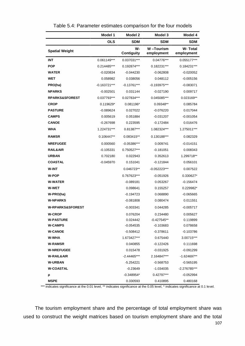
107

Table 5.4: Parameter estimates comparison for the four models

Model 1 Model 2 Model 3 Model 4

OLS SDM SDM SDM

Spatial Weight W-

Contiguity W –Tourism employment

W- Total employment

INT 0.061149*** 0.037031*** 0.04776*** 0.055177***

POP 0.214485*** 0.192874*** 0.182231*** 0.184231***

WATER -0.020834 -0.044230 -0.062808 -0.020052

WET 0.058982 0.038056 0.048112 -0.005156

PRO(ha) -0.163721*** -0.13761*** -0.193975*** -0.083071

NPARKS -0.002501 0.031144 -0.027190 0.009717

RPARKS&SFOREST 0.037793*** 0.027834*** 0.045085*** 0.023169**

CROP 0.119629* 0.081196* 0.09348** 0.085784

PASTURE -0.089624 0.027022 -0.076220 0.017044

CAMPS 0.005619 0.051884 -0.031207 -0.001054

CANOE -0.267698 0.223595 -0.172484 0.016476

WHA 1.224731*** 0.81387*** 1.082324*** 1.275011***

RAMSR 0.106447** 0.083415** 0.130188*** 0.082329

NREFUGEE 0.000560 -0.05386*** 0.009741 -0.014151

RAIL&AIR -0.105331 0.750527*** -0.181051 0.008343

URBAN 0.702180 0.022943 0.352613 1.299718**

COASTAL -0.045970 0.151041 -0.121844 0.056101

W-INT

0.046723** -0.052223*** 0.007522

W-POP

0.767623*** -0.051926 0.330627*

W-WATER

-0.089181 0.053267 -0.156474

W-WET

0.098641 0.155257 0.229982*

W-PRO(ha)

-0.194723 0.068890 -0.065665

W-NPARKS

-0.081808 0.080474 0.011551

W-RPARKS&SFOREST

-0.003341 0.044285 -0.005717

W-CROP

0.076204 0.234480 0.005627

W-PASTURE 0.024442 -0.427545** 0.119899

W-CAMPS

-0.054535 -0.103683 0.078658

W-CANOE

-0.508412 -0.378611 -0.103786

W-WHA

1.673427*** 0.675440 3.00715***

W-RAMSR

0.040855 -0.122426 0.111698

W-NREFUGEE

0.015478 -0.031925 -0.091299

W-RAIL&AIR

-2.44465*** 2.164847*** -1.624697**

W-URBAN

-5.254221 -0.568753 -0.565195

W-COASTAL

-0.23649 -1.034035 -2.276785***

ρ

-0.348954* 0.42797*** -0.052994

MSPE 0.330593 0.410895 0.480168


The tourism employment share and the percentage of total employment share was

used to construct the weight matrices based on tourism employment share and the total

108

employment share respectively (Tourism employment share and total employment share

matrices are provided in Table B3 and Table B4 of appendix of Chapter 5). Modified

versions of the sdm.m function from the Spatial Econometrics Toolbox were used to obtain

the parameter estimates of the all three spatial models.

5.4.5 Significance of the spatial correlation parameter (ρ)

The spatial correlation parameter, ρ, is significant in Model 2 and Model 3. In Model 2,

it is negative and significant at 10 per cent significance level while in Model 3 it is positive

and significant at 1 per cent significance level. Model 2 uses geographical neighbours and

Model 3 uses economic neighbours, when they have a similar regional profile based on the

share of employment from tourism. However, for Model 4 where the economic neighbours

are based on the share of total employment, the spatial correlation parameter was not

significant.

5.4.6 Point estimates

As explained in Section 4.5.2., the point estimates of the spatial regression model

cannot be used to draw conclusions on the existence of spatial dependence. As LeSage

and Pace (2009) explain, the partial derivative interpretation or the marginal effects is the

valid way of interpretation. The estimates on Table 5.4 are not marginal effects and thus the

magnitude of the effect cannot be assessed; however, the signs of these parameters

determine the sign of the marginal effects.

The estimates of the regression coefficients change when these parameters are

estimated jointly with different weight matrices by maximum likelihood method. It is important

to note that in all four models the results are consistent for amenity variables RPARKS &

SFORESTS (number of regional parks and state forests) and WHA (the existence of World

Heritage area) and are significant with a positive sign. This provides empirical evidence for

the importance of regional parks and state forests and World Heritage areas as tourism

amenities.

Further, except for Model 4, in all three models RAMSAR/DIWA (number of Ramsar

wetland and nationally important wetlands) and CROP (extent of croplands) are significant

at 10 per cent and 5 per cent significant levels and positive and PRO (percentage of total

protected area) is significant with negative sign (As shown in Table 5.4). This further

provides some insights on the significance of important wetlands and croplands as amenities

for tourists. There are two contributing amenity elements to Croplands; Croplands provide

109

some visual amenity and some croplands also contain vineyards, which can provide an

additional recreational factor to the tourists.

Similarly to CROP, RAMSAR/DIWA is significant and positive at 5 per cent and 1 per

cent significance levels in three models, except Model 4, which again demonstrates the

importance of these important wetlands as an amenity in tourism. Similarly, the protected

areas act as a dis-amenity on local tourism employment in the region. It is also important to

note that INT (percentage of people with Internet) and POP (estimated resident population),

are significant with the expected sign highlighting the importance of demography and

communication infrastructure on local tourism employment.

However, there are some differences on the signs and significance of the variables

across the three spatial models. In Model 2, in addition to above variables, NR (number of

nature refuge) and RAIL&AIR (existence of railway network and Airports) are also significant

with expected signs. The RAIL/AIR are significant with positive while NR was significant with

negative. NR is significant only in Model 2 and it is negative with 1 per cent significance

level. These refuge areas belong mainly to private landholders. Similarly to protected areas,

the results suggest nature refuge areas act as a dis-amenity to tourism as it is mainly belong

to private landholders there may be limited recreational activities for the tourists. Further, it

is important to note although beaches are one of the main natural tourist attractions in

Australia, particularly in Queensland, it has not being captured by the four models. One

explanation is that in several LGAs that border the coast also consist of the Great Barrier

Reef, World Heritage area.

5.4.7 Spatial spillover

When the explanatory variables interact with the spatial weights, they capture spatial

spillovers, which provide some insights on cross regional competitive and collaborative

effects.

In Model 2 the spatial effects are found significant, with W-INT, W-POP and W-WHA

being significant and positive, which suggests higher communication capacity, higher

population and existence of World Heritage areas in geographically close regions to provide

higher tourism employment in the given region. However, W-PRO, W-RAIL&AIR and W-

URBAN are significant and negative, which suggests higher percentage of protected areas,

existence of rail and airports; higher urban infrastructure in geographically neighbouring

110

regions also hinders the tourism employment in the given region. W-RAIL&AIR and W-

URBAN clearly indicate competition exists between geographically close neighbours.

In contrast, for Model 3 the spatial effect W-INT is significant and negative while W-

RAIL&AIR is significant and positive. This suggests better communication infrastructure

(proxied by the percentage of people with Internet) in neighbouring regions hinders the

tourism employment in the given region, while the existence of railway networks and airports

in neighbouring regions has a positive effect on the local tourism due to collaborative

operations between regions which are similar in tourism. This clearly indicates that

competitive and collaborative spillovers between regions vary based on the neighbourhood

structure.

In Model 4 where neighbours are defined as based on the share of total employment,

which captures the neighbourhood structure based on the economic performance (the share

of total employment as a proxy to economic performance of the region), W-INT, W-WET and

W-WHA are significant and positive, while W-RAIL&AIR and W-COASTAL are significant

and negative.

5.5 Direct, indirect and total effects

5.5.1 Decomposition of spatial effects of the explanatory variables into direct, indirect

and total effects

As described in Section 4.5.2, point estimates of the parameters of the spatial models

cannot be used to draw conclusions on the existence on spatial spillover. Inspection of the

expressions in equations (5.1) and (5.2) show the marginal effect; that is, the impact of a

change in a given independent variable is a function of the weights matrix and all the

parameters of the model.

𝑦 = (1 − 𝜌𝑊)−1 (𝑥𝛽 + 𝑊𝑥𝜃 + 𝜀) (5.1)

𝜕𝑦

𝜕𝑥 = (1 − 𝜌𝑊)−1 (𝛽 + 𝑊𝑥𝜃) (5.2)

The matrix of the partial derivatives of the expected value of y with respect to kth

explanatory variable x for the sample 1 to N is given by

111

(5.3)

Equation (5.3) illustrates the partial derivatives of 𝑦 with respect to the kth explanatory

variable having three important attributes. If a particular explanatory variable changes, the

dependent variable in that unit/region changes by (1 − 𝜌𝑊)−1𝛽, which is known as the direct

effect and appears in the diagonal. The off-diagonal elements show the effect of a change

in the kth explanatory variable for a given unit/region, on the value of the dependent variable

for other units/regions. This is known as the indirect effect which is measured by the cross

partial derivative which is (1 − 𝜌𝑊)−1𝑊𝜃.

(Elhorst (2014); LeSage and Pace (2009)) explain that the direct and indirect effects

are different for different units. Direct effects are different as (1 − 𝜌𝑊)−1 differs for different

units provided 𝜌 ≠ 0. The indirect effects are different because (1 − 𝜌𝑊)−1 as well as the 𝑊

is different for different units provided 𝜌 ≠ 0 and 𝜃 ≠ 0. The indirect effects if 𝜃 ≠ 0 is known

as local effects, and the indirect effects when 𝜌 ≠ 0 is known as global effects.

If both 𝜃 ≠ 0 and 𝜌 ≠ 0, both local and global effects exist but cannot be separated

from each other. As both direct and indirect effects are different for different units LeSage

and Pace (2009) describe a summary indicator for the direct effects as the average of the

diagonal elements of the matrix, and indirect effects as the average of either row sums or

column sums of the off-diagonal elements of the matrix. Hence, it is very important to note

the direct and indirect effects stated are an average value of the overall sample.

With respect to this study, direct and indirect effects are interpreted as follows; a

change in the single value of any explanatory variable will affect the region itself, which is

known as the direct effect and also might affect the neighbouring regions which is known as

1 1

1

1

1

( ) ( ).

( ) ( ). . . .

( ) ( ).

k Nk

k Nk

N N

k Nk

E y E y

x x

E Y E Y

x x

E y E y

x x

12 1

21 21

1 2

.

.( )

. . . .

.

k k N k

k k N k

N k N k k

w w

w wI W

w w

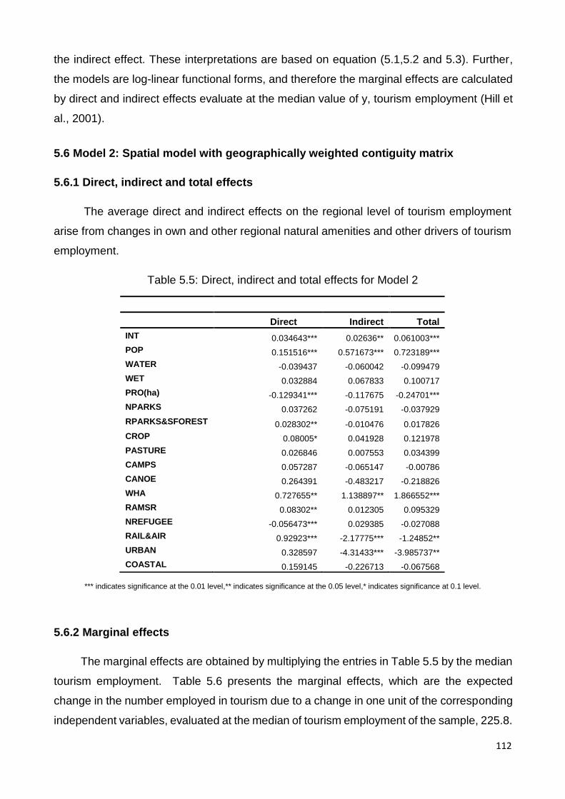
112

the indirect effect. These interpretations are based on equation (5.1,5.2 and 5.3). Further,

the models are log-linear functional forms, and therefore the marginal effects are calculated

by direct and indirect effects evaluate at the median value of y, tourism employment (Hill et

al., 2001).

5.6 Model 2: Spatial model with geographically weighted contiguity matrix


The average direct and indirect effects on the regional level of tourism employment

arise from changes in own and other regional natural amenities and other drivers of tourism

employment.

Table 5.5: Direct, indirect and total effects for Model 2

*** indicates significance at the 0.01 level,** indicates significance at the 0.05 level,* indicates significance at 0.1 level.

5.6.2 Marginal effects

The marginal effects are obtained by multiplying the entries in Table 5.5 by the median

tourism employment. Table 5.6 presents the marginal effects, which are the expected

change in the number employed in tourism due to a change in one unit of the corresponding

independent variables, evaluated at the median of tourism employment of the sample, 225.8.

Direct Indirect Total

INT 0.034643*** 0.02636** 0.061003***

POP 0.151516*** 0.571673*** 0.723189***

WATER -0.039437 -0.060042 -0.099479

WET 0.032884 0.067833 0.100717

PRO(ha) -0.129341*** -0.117675 -0.24701***

NPARKS 0.037262 -0.075191 -0.037929

RPARKS&SFOREST 0.028302** -0.010476 0.017826

CROP 0.08005* 0.041928 0.121978

PASTURE 0.026846 0.007553 0.034399

CAMPS 0.057287 -0.065147 -0.00786

CANOE 0.264391 -0.483217 -0.218826

WHA 0.727655** 1.138897** 1.866552***

RAMSR 0.08302** 0.012305 0.095329

NREFUGEE -0.056473*** 0.029385 -0.027088

RAIL&AIR 0.92923*** -2.17775*** -1.24852**

URBAN 0.328597 -4.31433*** -3.985737**

COASTAL 0.159145 -0.226713 -0.067568

113

Table 5.6: Marginal effects (Direct, indirect and total) for Model 2


RPARKS&SFOREST has a significant and positive direct effect at the 5 per cent level

of significance with no significant indirect effects. That is, the presence of a regional park or

State forest in a given region enhances tourism in that particular region with no influence on

neighbouring regions. One possible explanation is there is no unique contribution from a

given regional parks or State forest, as almost all LGAs have at least one of them. The

marginal effect is 6.37. Thus, one additional regional park or State forest leads to an

expected average increase in tourism employment of six employees, with no indirect effects

on geographically neighbouring regions.

WHA has significant direct and indirect effects at the 5 per cent significance level. The

direct is estimated to be 0.73 and the indirect effect is 1.14. As these are dummy variables,

these are semi-elasticity estimates. Thus, the existence of WHA in a region increases local

tourism employment by 73 per cent while in neighbouring regions by 114 per cent indicating

that due to the exclusive nature of this natural amenity, there are positive cross regional

spillover effects.


INT 7.79744*** 5.93310** 13.73055***

POP 34.1032*** 128.6721*** 162.7753***

WATER -8.87647996 -13.51425336

-22.39073332

WET 7.40153072 15.26785164 22.66938236

PRO(ha) -29.1120*** -26.486289 -55.5983***

NPARKS 8.38693096 -16.92399028 -8.53705932

RPARKS&SFOREST 6.37021** -2.35793808 4.01227608

CROP 18.0176* 9.43715424 27.45480824

PASTURE 6.04249768 1.70002924 7.74252692

CAMPS 12.89415796 -14.66328676 -1.769128

CANOE 59.50912628 -108.7624824 -49.253356

WHA 72.7655** 113.8897** 9.5329***

RAMSR 18.6872** 2.7696094 21.45665132

NREFUGEE -12.7109*** 6.6139758 -6.09696704

RAIL&AIR 92.923*** -217.775*** -124.852**

URBAN 32.8597 -431.4335*** -398.5737**

COASTAL 15.9145 -22.6713 -6.7568

114

RAMSAR/DIWA has a significant direct effect at the 5 per cent significance level and it

is estimated to be 0.083, where the direct marginal effect of RAMSAR/DIWA wetlands is

18.68. Thus one additional RAMSAR/DIWA wetland leads to an expected increase in

tourism employment of 19 employees in the local region with no significant influence on

neighbouring regions.

PRO (ha), which is the total protected area as a percentage of total population and NR

(nature refuge), also play an important role in regional tourism employment. As shown in

Table 4, both variables have negative and significant direct effects at 1 per cent significance

level with no indirect significant effects. That is, PRO (ha) and NR hinder tourism

employment in the given region. One possible explanation is that they do not provide any

recreational facilities for local tourism.

In addition to the natural amenity variables, RAIL&AIR (the existence of railway

network and airport) shows significantly positive direct effects and negative indirect effects

at the 1 per cent significance levels. As shown in Table 5.6, at the 1 per cent significance

level the direct effect is estimated to be 0.93 and indirect effect is 2.18. These effects could

be interpreted as semi-elasticity as these are dummy variables. That is, the existence of a

railway and airport in a region will enhance the local tourism employment by 93 per cent,

while hindering tourism employment in neighbouring region by 218 per cent.

It is important to stress that the indirect effects are both the local as well as the global

effects. Therefore, the possible explanations for the decreasing tourism employment may

be due to local effects; that is, cross regional competition of transport access infrastructure

as well as global effects: negative spillover from tourism employment. Further, in addition to

RAIL&AIR, URBAN (the intensity of “urbanness”) has significant negative indirect effects;

that is, being geographically neighbouring to a highly urban region hinders tourism

employment in a given region.

It is also evident that INT and POP have significant positive direct and indirect effects,

which shows that communication capacity of the region (the Internet) and the resident

population of a given region are important to tourism development for the region and its

neighbouring regions.

Finally it is important to note that the estimated spatial autocorrelation parameter, ρ, is

negative and significant at the 5 per cent level of significance, which indicates there is

competition for tourism employment across neighbouring regions. This result substantiates

115

the existing literature on tourism spillovers and the explanation of competitive effects

between regions for tourists (Pavlyuk, 2010, 2011a).

5.7 Model 3: neighbourhood structure based on share of tourism employment


Tables 5.7 and 5.8 present the direct, indirect and total effects, and marginal effects,

respectively, for Model 3.



INT 0.042704*** -0.055129* -0.012425

POP 0.185043*** 0.036616 0.221659

WATER -0.061968 0.037808 -0.024161

WET 0.074466 0.285909 0.360375

PRO(ha) -0.196587*** -0.02066 -0.217247

NPARKS -0.015927 0.113228 0.097301

RPARKS&SFOREST 0.054847*** 0.107753** 0.162601***

CROP 0.136086** 0.461995 0.598081

PASTURE -0.147181* -0.769874* -0.917055*

CAMPS -0.050221 -0.203001 -0.253222

CANOE -0.239273 -0.730434 -0.969706

WHA 1.264048*** 1.986907 3.250955**

RAMSR 0.121894** -0.101949 0.019945

NREFUGEE 0.004177 -0.052348 -0.048172

RAIL&AIR 0.140487 3.534139*** 3.674626**

URBAN 0.280627 -0.577933 -0.297306

COASTAL -0.278738 -1.841668 -2.120407


116

Table 5.8: Marginal effects of Model 3


INT 9.61182*** -12.40843* -2.796619

POP 41.6494*** 8.24152928 49.89100772

WATER -13.94775744 8.50982464 -5.43815788

WET 16.76080728 64.35239772 81.113205

PRO(ha) -44.2478*** -4.6501528 -48.89795476

NPARKS -3.58484916 25.48535824 21.90050908

RPARKS&SFOREST 12.3449*** 24.2530** 36.5982***

CROP 30.6302** 103.9858346 134.6160715

PASTURE -33.1274* -173.2832* -206.4107*

CAMPS -11.30374268 -45.69146508 -56.99520776

CANOE -53.85556684 -164.4060847 -218.2614265

WHA 126.4048*** 198.6907 325.0955**

RAMSR 27.4359** -22.94668092 4.4892206

NREFUGEE 0.94015916 -11.7824*** -10.8425**

RAIL&AIR 14.0487 353.4139*** 367.4626**

URBAN 28.0627 -130.0811596 -29.7306

COASTAL -27.8738 -414.5226334 -212.0407


RPARKS&SFOREST has significant and positive direct and indirect effects at the 1 per

cent and 5 per cent level of significance, respectively. This indicates that the presence of

regional parks and state forests in a given region enhances tourism in that particular region,

as well as in the neighbouring regions with similar tourism performance. The direct effect is

estimated to be 0.0549 and the marginal effect is 12.4. Thus, one additional regional park

leads to an expected average increase in tourism employment of 12 employees.

The indirect effect is estimated to be 0.1078 and marginal indirect effect is 24.25. That

is, one additional regional or State forest leads to an expected average increase in tourism

employment by 24 employees in the neighbouring region. Further, it is noted that the total

effects of RPARKS and SFFOREST are significant at 1 per cent. The total effect is the sum

of direct and indirect effects. The total effects of RPARKS is estimated to be 0.01626 and

marginal total effect is 36.5. This can be interpreted as one additional regional park or State

forest is expected to increase tourism employment by 37 employees when counting those

in the direct location and those that are generated in the neighbouring regions.

The results also suggest a significant role of World Heritage areas in tourism

employment. The direct effect is estimated to be 1.26; as the variable is binary, this indirect

117

effect can be interpreted as semi-elasticity. Thus, the existence of WHA in a region increases

local tourism employment by 126 per cent.

RAMSAR/DIWA is a significant direct effect at the 5 per cent significance level and it is

estimated to be 0.121894 and the marginal effect of RAMSAR/DIWA wetlands indicating an

expected increase in tourism employment of 27 employees in the local region. However,

there are no significant indirect effects to neighbouring regions.

PRO (ha), which is the total protected area as a percentage of total population also

plays an important role in regional tourism employment. As shown in Table 5.8, it has a

negative and significant direct effect at the 1 per cent significance level with no indirect

significant effects. That is PRO (ha) in a given area, tends to act as a disamenity to a given

region. This is further validated, as, although these provide green areas to the region, they

do not provide any recreational facilities to the local tourism, which is consistent with existing

literature.

In addition to the natural amenity variables, RAIL&AIR have significant, positive and

substantial indirect and total effects at the 1 per cent significance levels. As shown in Table

5.8, at the 1 per cent significance level the indirect effect is estimated to be 3.534 and total

effect of 3.675. These effects could be interpreted as semi-elasticity. That is, the existence

of a railway and airport in a region will enhance the tourism employment in the neighbouring

regions by 353.4 per cent. In addition, INT, which captures the communication capacity of

the region, has significant positive direct effect with significant negative indirect effects.

However, it is important to note the indirect effects from RAIL&AIR are negative and

significant when neighbours are defined by geographical proximity (Model 2) (see Table

5.5). This further confirms the competitive and collaboration effects between regions at

different neighbourhood structures.

CROP and PASTURES have significant positive and negative direct effects

respectively. One possible explanation is the definition of the variables. For instance, the

presence of winery or vineyards (which is a tourist attraction) within the agricultural lands is

not separately defined but would be included in CROP in this study.

INT has significant positive direct and negative indirect effects, which shows that the

communication capacity of the region (Internet) enhances tourism in that given region, but

hinders tourism performance in neighbouring regions. The result highlights two effects. The

first is that well-connected regions can reach potential tourists through an array of options

118

(for example, social media and websites) that rely on good Internet connectivity. The second

is that tourists increasingly prefer to be connected while on holidays. POP (estimated

resident population) has significant positive direct effects; that is, the resident population

contributes positively to local tourism employment, which is consistent with the existing

literature.

Most importantly, spatial autocorrelation parameter, ρ, is positive and significant at the

1 per cent level of significance. This is a positive correlation in tourism employment across

neighbouring regions that are economically close. The possible explanation is that there are

collaborative spillover effects, which may be “market access spillovers” and “joint promotion

spillover” between regions (Yang and Wong (2012)).

5.8 Comparison of Models 2 and 3

One of the most interesting outcomes of this analysis is that the spatial correlation

parameter, ρ, is significant but of opposite signs in Models 2 and 3: ρ is negative for Model

2 and positive in Model 3. This indicates the interaction between geographically close

regions is one of competition, while that of regions with similar share of tourism is

collaborative. The results are consistent with existing literature on tourism (Park and Yoon,

2011; Pavlyuk, 2011b; Yang and Wong, 2012).

RPARKS&SFOREST has no significant indirect effects in geographic neighbours

(Model 2) while there are significant positive indirect effects in Model 3 where neighbours

with similar tourism performance. This again indicates the collaborative and competitive

effects between two different types of neighbours. The results indicate more regional parks

and state forests in neighbouring regions with similar tourism performances will promote

tourism employment in a given region, while regional parks and state forests have no effects

on geographically close neighbours.

The presence of WHA has significant direct positive effects in both models with

significant positive indirect effects in model with geographic neighbours. However, it is

important to note that although the presence of WHA has no statistically significant indirect

effects in model with similar tourism performance, the total effect is significant and positive.

Therefore, this indicates that regardless of the neighbourhood structure, the presence of

World Heritage sites demonstrates significant and positive contribution to tourism

employment spillover.

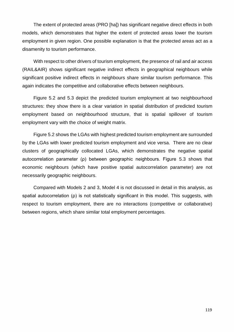
119

The extent of protected areas (PRO [ha]) has significant negative direct effects in both

models, which demonstrates that higher the extent of protected areas lower the tourism

employment in given region. One possible explanation is that the protected areas act as a

disamenity to tourism performance.

With respect to other drivers of tourism employment, the presence of rail and air access

(RAIL&AIR) shows significant negative indirect effects in geographical neighbours while

significant positive indirect effects in neighbours share similar tourism performance. This

again indicates the competitive and collaborative effects between neighbours.

Figure 5.2 and 5.3 depict the predicted tourism employment at two neighbourhood

structures: they show there is a clear variation in spatial distribution of predicted tourism

employment based on neighbourhood structure, that is spatial spillover of tourism

employment vary with the choice of weight matrix.

Figure 5.2 shows the LGAs with highest predicted tourism employment are surrounded

by the LGAs with lower predicted tourism employment and vice versa. There are no clear

clusters of geographically collocated LGAs, which demonstrates the negative spatial

autocorrelation parameter (ρ) between geographic neighbours. Figure 5.3 shows that

economic neighbours (which have positive spatial autocorrelation parameter) are not

necessarily geographic neighbours.

Compared with Models 2 and 3, Model 4 is not discussed in detail in this analysis, as

spatial autocorrelation (ρ) is not statistically significant in this model. This suggests, with

respect to tourism employment, there are no interactions (competitive or collaborative)

between regions, which share similar total employment percentages.

120

Figure 5.2: Spatial Distribution of predicted tourism employment under geographic matrix

121

Figure 5.3: Spatial Distribution of predicted tourism employment under tourism share

matrix

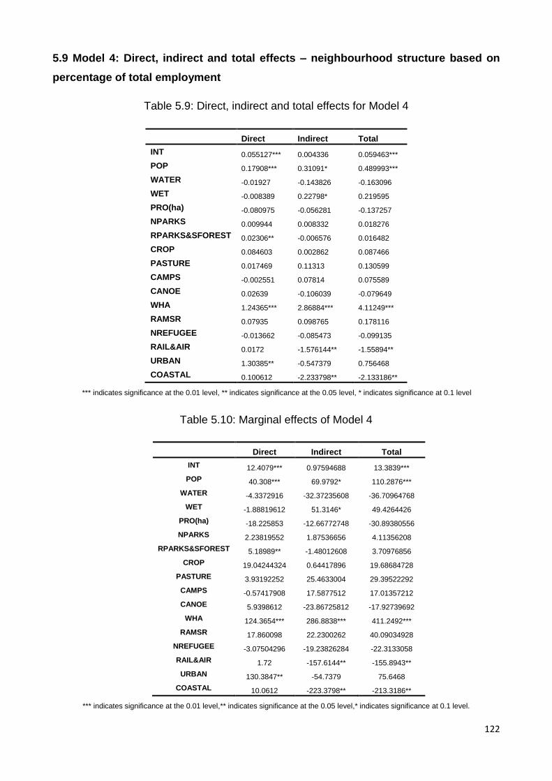
122

5.9 Model 4: Direct, indirect and total effects – neighbourhood structure based on

percentage of total employment



INT 0.055127*** 0.004336 0.059463***

POP 0.17908*** 0.31091* 0.489993***

WATER -0.01927 -0.143826 -0.163096

WET -0.008389 0.22798* 0.219595

PRO(ha) -0.080975 -0.056281 -0.137257

NPARKS 0.009944 0.008332 0.018276

RPARKS&SFOREST 0.02306** -0.006576 0.016482

CROP 0.084603 0.002862 0.087466

PASTURE 0.017469 0.11313 0.130599

CAMPS -0.002551 0.07814 0.075589

CANOE 0.02639 -0.106039 -0.079649

WHA 1.24365*** 2.86884*** 4.11249***

RAMSR 0.07935 0.098765 0.178116

NREFUGEE -0.013662 -0.085473 -0.099135

RAIL&AIR 0.0172 -1.576144** -1.55894**

URBAN 1.30385** -0.547379 0.756468

COASTAL 0.100612 -2.233798** -2.133186**

*** indicates significance at the 0.01 level, ** indicates significance at the 0.05 level, * indicates significance at 0.1 level

Table 5.10: Marginal effects of Model 4


INT 12.4079*** 0.97594688 13.3839***

POP 40.308*** 69.9792* 110.2876***

WATER -4.3372916 -32.37235608 -36.70964768

WET -1.88819612 51.3146* 49.4264426

PRO(ha) -18.225853 -12.66772748 -30.89380556

NPARKS 2.23819552 1.87536656 4.11356208

RPARKS&SFOREST 5.18989** -1.48012608 3.70976856

CROP 19.04244324 0.64417896 19.68684728

PASTURE 3.93192252 25.4633004 29.39522292

CAMPS -0.57417908 17.5877512 17.01357212

CANOE 5.9398612 -23.86725812 -17.92739692

WHA 124.3654*** 286.8838*** 411.2492***

RAMSR 17.860098 22.2300262 40.09034928

NREFUGEE -3.07504296 -19.23826284 -22.3133058

RAIL&AIR 1.72 -157.6144** -155.8943**

URBAN 130.3847** -54.7379 75.6468

COASTAL 10.0612 -223.3798** -213.3186**


123

5.10 Prediction of tourism employment

The primary purpose of the model is to predict tourism employment in each LGA at

different neighbourhood structures and to select the best model. Hence, accuracy of

prediction is critical when comparing competing models. The Mean Square Prediction Error

(MSPE) is commonly used as a simple criterion to test the predictive ability of a model.

MSPE is defined by:

𝑀𝑆𝑃𝐸 = 𝐸(𝑦 − �̅�)2 ……………………………………………(5.4)

𝐸 denotes the expectation over the target population of individual observations.

Considering the sample of size n, and denoting the predicted value of 𝑦𝑖 by �̂�𝑖 𝑖 = 1, … , 𝑛,

the MSPE is given by :

𝑀𝑆𝑃𝐸 = (1

𝑛) ∑ (𝑦𝑖 − �̂�𝑖 )

2

𝑖 ………………………………………….(5.5)

Then the model with the lowest MSPE will be selected as the best model for the

prediction. As described in Table 5.5B appendix for Chapter 5, Model 2 has the lowest Mean

Square Prediction Error (MSPE), which is 0.330593, compared with 0.410895 and 0.480168

in Models 3 and 4 respectively, thus it would be the most suitable model to predict tourism

employment. A detailed calculation of MSPE for each model is presented in Table 5.5B

appendix for Chapter 5.

5.11 Robustness of the model under different neighbourhood structure

Table 5.11 provides a comparison of the estimated spatial effects across the three

spatial models. While the spatial autoregressive parameter, , and the indirect effects of the

explanatory variables vary with the choice (which is in line with previous research) the

parameter estimates and direct spatial effects are not sensitive to the choice of the spatial

weight matrix.

However, as described in Section 5.5, the direct effects and indirect effects are different

for different units (LGAs in this study) as the term (1 − 𝜌𝑊)−1 is different across models.

The Table 5.11 provides only the average direct and indirect effects.

124

Table 5.1113: Sensitivity of results to the choice of neighbour definition


An investigation of the influence of mining on tourism employment in regional

Queensland in provided in the next section. As discussed in Chapter 1, with the recent

downturn of mining in Australia including Queensland, this study considers tourism

employment as a strong contender for potential employment opportunities in those affected

areas by mining sector. Hence, it is important to examine the co-existence of mining and

tourism in regional Queensland.

5.12 Impact of mining on regional tourism in 2011

As explained in Section 4.12, in order to examine the influence of mining on tourism

employment, a dummy variable, reflecting mining activity in each LGA is incorporated into

each of the four models. The dummy variable, MINE, equals “1” if the percentage of mining

employment out of total employment in the region is more than 10 per cent in that region,

and “0” otherwise. It is important to note that the variable capturing mining may influence

tourism in two ways. First, mining activity may influence tourism performance. Second,

mining employment may influence tourism employment due to higher demand in areas such

as hospitality. Maximum likelihood estimates of the parameters are presented in Table 5.12.

The models are described below:

Model 1M: The base model with simple non-spatial regression model with MINE as a

variable

13 Entries which are not included are as not significant at any level. Table 5.6B is in appendix with the all entries

Model 3 Model 4

Direct Indirect Total Direct Indirect Total Direct Indirect Total

INT 0.034643*** 0.02636** 0.061003*** 0.042704*** 0.055127*** 0.059463***

POP 0.151516*** 0.571673*** 0.723189*** 0.185043*** 0.179084*** 0.310908* 0.489993***

WATER

WET 0.227984*

PRO(ha) (-0.129341***) (-0.247016***) (-0.196587***)

NPARKS

RPARKS&S

FOREST 0.028302** 0.054847*** 0.107753** 0.162601*** 0.023058*

CROP 0.08005* 0.136086**

PASTURE (-0.147181*) (-0.769874*) (-0.917055*)

CAMPS

CANOE

WHA 0.727655** 1.138897** 1.866552*** 1.264048*** 3.250955** 1.243654*** 2.868838*** 4.112492***

RAMSR 0.08302** 0.121894**

NREFUGEE (-0.056473***)

RAIL&AIR 0.92923*** (-2.17775***) (-1.24852**) 3.534139*** 3.674626** (-1.576144**)(-1.558943**)

URBAN 0.328597 (-4.314335***)(-3.985737**) 1.303847**

COASTAL (-2.233798**)(-2.133186**)

Model 2

125

Model 2M: Spatial model with geographically weighted contiguity matrix with MINE as a

variable;

Model 3M: Spatial model with weight matrix based on share of tourism employment with

MINE as a variable;

Model 4M: Spatial model with weight matrix based on total employment percentage with

MINE as a variable;

5.13 Significance of the spatial auto correlation parameter (ρ)

As shown in Table 5.12, the results suggest the significance and the sign of the mining

variable vary with the neighbourhood structure; however, the spatial autocorrelation

parameter (ρ) is significant only at 1 per cent significance level only in Model 3M, where

neighbours are defined as those with similar regional profile with respect to their share of

tourism employment. Similarly to the results obtained in Model 3 (without the mining

variable), in Model 3M, a positive spatial auto correlation is observed. This indicates positive

cross regional tourism employment spillovers. That is, when two LGAs are close neighbours,

with respect to tourism employment there are agglomeration effects; namely, collaboration

and joint promotion between the two regions which provide positive cross regional spillovers

in tourism employment irrespective of mining activities in the regions.

In contrast to Model 3M, in Model 2M and Model 4M, where neighbourhood structures

are based on geographical proximity and share of total employment, respectively, the ρ is

not significant indicating no significant cross regional spatial spillovers in tourism

employment between geographical neighbours. As noted with Model 2 (Model without the

mining variable and neighbours are defined based on geographical proximity) the spatial

autocorrelation parameter (ρ) was significant and negative indicating negative tourism

employment spillovers across geographical regions, which is in contrast to the non-

significant results obtained when the mining variable is included. This provides some useful

insights into the interaction (co-existence) of tourism and mining industry.

126

Table 5.12 Parameter estimates comparison for the four models


Model 1M Model 2M Model 3M Model 4M

OLS SDM SDM SDM

Spatial Weight W-Geographic

W –Tourism employment

W- Total employment

INT 0.061649*** 0.03829*** 0.048789*** 0.058689***

POP 0.218629*** 0.190548*** 0.18967*** 0.197372***

WATER -0.021069 -0.034057 -0.064406 -0.025477

WET 0.061367 0.041255 0.052752 0.021657

PRO(ha) -0.16187*** -0.12535*** -0.186937*** -0.096889

NPARKS -0.000713 0.035281 -0.022589 0.020058

RPARKS&SFOREST 0.038019*** 0.026659** 0.045888*** 0.024297**

CROP 0.123570 0.084851* 0.101632** 0.116475*

PASTURE -0.102608 -0.013332 -0.108608 -0.055015

CAMPS -0.004602 -0.000576 -0.062105 -0.046740

CANOE -0.272321 0.208307 -0.195011 0.005078

WHA 1.232093*** 0.82849*** 1.104836*** 1.299367***

RAMSR 0.105643** 0.075053** 0.127664*** 0.083916

NREFUGEE 0.000818 -0.044949** 0.011986 -0.016352

RAIL&AIR -0.115443 0.695221** -0.215737 0.024009

URBAN 0.634447 -0.128747 0.164876 0.945396

COASTAL -0.034170 0.273050 -0.081774 0.099473

MINE 0.130183 0.288789 0.345021 0.601991*

W-INT 0.039447** -0.05198*** 0.011779

W-POP 0.695393*** -0.053881 0.339967**

W-WATER -0.083144 0.054377 -0.194239

W-WET 0.067251 0.163672 0.292915**

W-PRO(ha) -0.178138 0.085083 -0.107063

W-NPARKS -0.079564 0.071506 0.018307

W-RPARKS&SFOREST

-0.009138 0.047995* -0.004177

W-CROP

0.019912 0.228500 0.066918

W-PASTURE

0.163884 -0.441356* 0.010354

W-CAMPS

-0.012850 -0.056131 0.088297

W-CANOE

-0.327620 -0.382081 -0.033276

W-WHA

1.401555** 0.639923 3.098137***

W-RAMSR

0.024021 -0.143186 0.102979

W-NREFUGEE

-0.005360 -0.035304 -0.105784

W-RAIL&AIR

-2.28199*** 2.212038*** -1.703081**

W-URBAN

-4.76572*** -0.582511 -0.831243

W-COASTAL

-0.185597 -1.086647 -2.316861***

W-MINE

-1.081098* -0.080056 0.462669

ρ -0.239983 0.430996*** -0.060995

127

5.14 Parameter estimates of the models with the mining variable

Although point estimates cannot be used to draw conclusions about the spatial

spillovers, the variable MINE is significant only in Model 4M, where the neighbourhood

structure is based on the share of total employment, and W-MINE is significant and negative

only in Model 2M where neighbours are defined, as based on geographical contiguity.

In all four models the results are consistent for amenity variables RPARKS&

SFORESTS (number of regional parks and state forests), WHA (existence of World Heritage

area) are significant with positive sign similarly to models without the mining variable. With

the exception of Model 4M, in all other three models PRO (percentage of total protected

area) is significant with negative sign with RAMSAR/DIWA is significant and positive

similarly to the models without the mining variable.

In addition to the above variables, the significance and the sign of the variables in all

four models are consistent with the results obtained in models without the mining variable.

This further demonstrates the robustness of the model specification and gives some insights

on influence on mining on regional tourism employment.

5.15 Significance of the mining variable

5.15.1 Model 2M

As explained in Section 5.5 when the explanatory variables are interacted with the

spatial weights, they capture spatial spillovers, which reflects the cross regional competitive

and collaborative effects. In Model 2M, W-MINE is negative and significant at the 10 per cent

significance level. The results suggest that higher mining employment (>10 per cent) in

geographically neighbouring regions hinders tourism employment in a given region.

With respect to the decomposition of the spatial effects of the explanatory variables

into direct, indirect and total effects, MINE has a significant negative indirect effect at the 10

per cent significance level with no direct effects on tourism employment. This indicates

higher mining employment in the neighbouring regions has a significant and negative

influence on tourism employment in a given region.

One possible explanation is that when compared with tourism, mining is higher-paid

and it therefore acts as a ‘pull factor’ for employment. That is, it has a labour-based

competition effect in the regional labour market. In addition to W-MINE, W-URBAN is also

negative and significant at the 10 per cent percent significance level. As described above

128

this provide interesting insights into the interaction (co-existence) of tourism and mining

industry. When mining is included the spatial autocorrelation parameter (ρ) is not significant

and negative as without the mining variable. But in contrast W-MINE is significant and

negative.

5.15.2 Model 3M

As shown in Table 5.12, in Model 3M (where the neighbourhood structure is based on

the share of tourism employment) mining does not contribute to tourism employment either

as a single variable (MINE) or as a spatially lagged independent variable W-MINE. Further,

as shown in Table 5.13, the influence of mining on the direct effects, indirect effects and

total effects is also insignificant. However, as in Model 3, the spatial autocorrelation

parameter (ρ) is significant and positive. Hence, the results are that when the neighbourhood

structure is defined as based on the share of tourism employment, there is no significant

direct or spillover effects on tourism employment from mining.

5.15.3 Model 4M

As shown in Table 5.12, the point estimator of MINE is significant and positive while

W-MINE is not significant. That is, if mining employment is higher (>10 per cent) in a given

region, it positively contributes to tourism employment in the given region with no influence

on tourism employment in neighbouring regions, which is consistent with existing literature

on the competitive and coexistence context between mining and tourism (Buultjens J. et al.,

2010)

One possible explanation is that mining through increased infrastructure may

advantage tourism. Further, as shown in Table 5.13, in Model 4M, in addition to the

significant direct and indirect effects described in Model 4 (without mining variable), MINE

has a positive and significant direct effect at the 10 per cent significance level with no

significant indirect effects. The results suggest that for two regions that are close economic

neighbours (measured by their share of total employment), the presence of mining

contributes to increase regional tourism employment.

However, it is important to note that the direct effects and indirect effects are different

for different LGAs in the sample, and the direct and indirect effects shown in the Table 5.13

are the average direct and indirect effects over all LGAs. Further, this analysis uses the

percentage of employment in mining to capture mining performance of a region; however,

there may be other factors, such as environmental pollution and the provision of

129

infrastructure that reflects mining performance of the region, which were not taken into

account in this analysis.

Table 5.13 Direct, indirect and total effects


5.16 Conclusions

In this chapter, tourism employment data in 74 LGAs in the State of Queensland are

gathered and analysed for each Local Government Area (LGA) in the state based on the

methodology described in Section 4.3.1, using information TSA 2011-2012(Pham and

Kookana, 2013) and ABS 2011 Census Community profile (Basic Community Profile

(Catalogue number 2001.0)).

Based on the results obtained in diagnostic tests for the presence of a spatial lag and

spatial errors, it is concluded that the Spatial Durbin Model (SDM) is the most appropriate

spatial model for this study. Alternative specifications of SDMs are estimated using three

alternative definitions of neighbours to construct the spatial weight matrices, namely:

geographic weight matrix (to capture the geographic proximity between

regions);

Model 3M Model 4M

Direct Indirect Total Direct Indirect Total Direct Indirect Total

INT 0.03729*** 0.025135* 0.06243*** 0.0437*** (-0.0534*) 0.05831*** 0.00804* 0.06634***

PO P 0.16511*** 0.55482*** 0.719932*** 0.19473*** 0.18974*** 0.31068 0.50043***

WATER

WET 0.2858*

PRO (ha) (-0.12087***) -0.12207 (-0.24295***) (-0.1878**)

NPARKS

RPARKS&

SFO REST 0.02685** 0.0555*** 0.113126** 0.168631*** 0.0240**

CRO P 0.1377**

PASTURE (-0.1720*) (-0.791497*) (-0.96350*)

CAMPS

CANO E

WHA 0.77823*** 1.003586** 1.78182*** 1.27628*** 3.196449** 1.2361*** 2.92238** 4.15851***

RAMSR 0.07574** 0.11616**

NREFUGEE (-0.04515**)

RAIL/AIR 0.79071*** (-2.06575***)(-1.275043**) 3.53582*** 3.624806* (-1.64098**) (-1.59291**)

URBAN (-4.065198***) -4.00699

CO ASTAL (-2.24310**) (-2.1041**)

MINE (-1.020627*) 0.587649*

Model 2M

130

weight matrix defined by the share of tourism employment (to capture the

proximity based on tourism performance); and

weight matrix defined by the percentage of total employment (to capture the

proximity based on economic performance).

Under all specifications (spatial and non-spatial) the percentage of population with

Internet (INT), estimated regional population (POP), number of regional parks and State

forest (RPARKS&SFOREST) and World Heritage areas (WHA) has been found to be

statistically significant and this is taken as evidence of their importance as factors that

influence tourism employment in a region. However, the magnitude of the effects varies

across the three spatial specifications. This is consistent with other studies (Pijnenburg and

Kholodilin, 2014), which suggests spatial spillover effects may vary, based on the assigned

neighbourhood structure chosen.

With respect to spillovers, the results suggest the spillovers vary with the type of

neighbourhood structure or the weight matrix. RPARKS&SFOREST shows no significant

indirect effects in geographic neighbours, while significant positive spillovers are in Model 3,

where neighbours have similar tourism performance. This indicates the collaborative and

competitive effects between two different types of neighbours.

The presence of WHA shows significant positive indirect effects in Model with

geographic neighbours with no statistically significant indirect effects in model with similar

tourism performance. However, the total effects of presence of WHA are significant and

positive in the model with similar tourism performance neighbourhood structure. Therefore,

this indicates that regardless of the neighbourhood structure, presence of World Heritage

sites demonstrate significant and positive contribution to tourism employment.

The extent of protected areas (PRO[ha]) has significant negative direct effects in both

models, which demonstrates that the higher the extent of protected areas lower the tourism

employment in given region. One possible explanation is that protected areas act as a

disamenity to tourism performance.

The presence of rail and air access (RAIL&AIR) shows significant negative indirect

effects in geographical neighbours, while significant positive indirect effects in neighbours

share similar tourism performance. This again indicates the competitive and collaborative

effects between neighbours.

131

The findings also show the spatial autocorrelation (ρ) is negative and significant

between regions of geographical proximity, which captures competition for tourism

employment between regions. With a similar argument, Pavlyuk (2010) find negative spatial

autoregressive lag parameter of employment rates between regions with geographical

proximity due to competition between regions in Baltic states. Further Pavlyuk (2011a) finds

negative spatial autoregressive lag parameter of number of tourists between regions in

Baltic states, which again demonstrates the competition between geographical neighbours

with respect to tourists.

However, Chhetre et al. (2013) find positive spillovers between geographic neighbours

only when Tourism and Hospitality (T&H) employment is considered. One possible

explanation is that the study considered T&H employment which is a sub component of total,

direct and indirect tourism employment based on Tourism Satellite Accounts.

However, the spatial autocorrelation (ρ) is significant and positive when proximity is

defined as regions that are similar in their share of tourism employment, indicating

collaboration effects between regions with similar tourism performance. The best

performing model, in terms of prediction of tourism employment, is the one where the

neighbourhood structure used is based on geographic proximity. This model with the

geographical proximity neighbourhood structure had the lowest mean square prediction

error amongst competing specifications.

With respect to the influence of mining on tourism employment, a dummy variable

MINE was incorporated into all four models, including the non-spatial base model. The

results indicate the mining industry produces negative spillovers to neighbouring regions

when neighbours are defined by geographical contiguity.

The results of this research provide several important policy implications for regional

tourism planners and decision-makers, which is discussed in Chapter 7 of this thesis.

132

Chapter 6

Identifying proximity dimensions or neighbourhood structures in tourism employment clusters

6.1 Introduction

As described in Section1.4, this thesis aims to address three objectives and this

chapter intends to investigate objective Number 3; that is, to investigate whether there are

tourism employment clusters in regional Queensland and if so, to investigate the

characteristics and the type of proximity dimension or the neighbourhood structure that links

them together as a cluster. Hence, this chapter analyses empirically the characteristics and

proximity dimensions of spatial clustering of tourism employment in Queensland for 2011.

Clusters or agglomeration economies enhance regional industry performance through

positive multiplier effects and the positive externalities that are derived as a result of

geographical concentration or agglomeration of similar industries. Clusters increase the

competitiveness and corporate-ness between co-located symbiotic industries. Although

spatially fragmented global economies are becoming increasingly common, it is evident that

the adoption of cluster theory enhances the economies through fostering the collaborative

and joint sharing of common resources (Chhetre et al., 2013; Michael, 2003).

To date, cluster theory has largely been applied in the manufacturing sector, although

there is some evidence in the literature of the application of cluster theory in service-based

industries, such as tourism (Chhetre et al., 2013; Estêvão and Ferreira, 2009; Jackson and

Murphy, 2002, 2006; Vladimirovna et al., 2015).

The use of cluster-based modelling to analyse tourism industry has already proved to

be useful tool in regional growth and regional tourism analysis. The development of clusters

with homogeneous elements could be a viable strategy for economic growth and to harness

tourism development opportunities (Chhetre et al., 2013; Chhetre et al., 2016; Hall and

Michael, 2007).

Geographical agglomeration or clustering based on geographical proximity is well

theorised in regional studies and economic geography, which suggests the co-location of

industries and firms provides competitive advantages. However, the use of alternative

proximity dimensions or neighbourhood structures of clustering to investigate linkages

between different sectors is limited in literature. As described in Part 2 of literature review in

Chapter 4, geographical proximity is not the only type of proximity used to represent

133

interactions. Other types of proximity dimensions include social proximity, cognitive

proximity and institutional proximity (Boschma, 2005).

Although there is evidence of the application of cluster theory in the tourism studies, it

has only been applied to clustering based on geographic proximity, where clusters are

defined according to Potter’s cluster theory (Porter, 2000). However, if there is clustering

based on another proximity dimension (and not only on geographical proximity), this should

be taken into account when designing any policies and strategies for regional economic

growth and development of tourism.

The cluster-centred growth model in tourism is critical as a tool in regional economic

development, and this chapter provides a broader perspective and assists in the

development of plans or strategies based on clustering in regional development. This

chapter examines economic proximity dimensions that exist in tourism employment and the

key characteristics of the clusters that are identified.

6.2 Literature review: background

Industry-level clustering is theorised in regional studies in the economic geography

literature, where geographic proximity facilitates competition and

collaboration/agglomeration between industries (Porter, 2000).Clusters are geographic

agglomerations of interconnected companies, or services, firms, industries or institutions in

a particular field, which compete, as well as cooperate with each other. This competitiveness

and collaborative-ness of the clusters creates competitive advantages over outside

companies and stimulates economic growth in the region.

Although until recently, clusters were defined based on geographical concentration of

similar industries, recent literature suggests, proximity can be defined beyond geographical

distance (Autant-Bernard and LeSage, 2011; Parent and LeSage, 2008; Pijnenburg and

Kholodilin, 2014; Rambaldi et al., 2010). Hence, it is important to explore other proximity

dimensions in clustering.

The following sections discuss the concepts of clusters based on a traditional

perspective, non-traditional, and non-geographical concentrated clusters in the existing

literature. Although the focus of this chapter is to investigate non-geographic proximity

dimensions in tourism employment clusters, this chapter starts with a definition of the cluster

concept.

134

6.3 Theoretical foundation of clusters

6.3.1 The New Economic Geography (NEG)

The new economic geography is the study that ‘houses’ the geographical perspective

of clustering. Since the late 1970s, Paul Krugman has pioneered locating geography within

the economic context. ‘New economic geography’ is the study of the agglomeration or

clustering as a result of increasing returns to scale and transportation costs and linkages of

firms between their suppliers and customers. Many economic activities are noticeably

concentrated geographically and there are forces that promote concentration and oppose

concentration; these are centripetal and centrifugal, respectively. The centripetal forces

include market size and linkages, thick labour markets (employees finding it easy to get

work) and external economies through information spillovers.

The centrifugal factors are immobile factors (land and natural resources), land rents

and external diseconomies. Increasing housing cost, commuting time, degradation of

environment and crime are also included as centrifugal factors of agglomeration. The

agglomeration economies discuss three types of externalities, which are localisation

economies, urbanisation economies and Jacobs’ externalities (Frenken et al., 2007).

Localisation economies are formed by agglomeration externalities operating within an

industry and by local concentration of that industry. Urbanisation economies are developed

due to urban size and density. Jacobs’ externalities arise as a result of a local variety of

producers (Yang, 2012).

Economic geography does not describe the interactions and positive spillovers

between firms that are advanced by agglomeration. The theory of clustering describes the

interaction across firms or industries. New economic geography concentrates on an

agglomeration of economic activity within a particular industry, while cluster theory focuses

on interactions across industries. Therefore, cluster theory is built on economic geography

and considered to be a field in economic geography(Krugman, 1998; Smith, 2012).

6.3.2 Cluster theory: Clusters based on geographic proximity

Clusters are considered to be part of the economic landscape, with geographic

agglomeration of elements of a particular industry, the theory of cluster concept dates back

at least to Marshall (1890/1920) who describes the externalities of specialised industry

135

locations in Principles of Economics14 (Porter, 2000). The concept of cluster theory became

more prominent with Porter’s The Competitive Advantage of Nations (1990), in which he

discusses the importance of clusters in national, state and local level competitiveness in

global economy.

According to Porter (2000), clusters are geographic concentrations (geographic

proximate) of groups or agglomerations of companies or institutions in a particular activity

sector, and are linked by commonalities and complementarities in which their interactions

enhance the competitive advantage. Clusters consist of an array of interconnected

industries and other units that are important for competition. They include suppliers of

specialised inputs, providers of specialised infrastructure, and manufacturers of

complementary products, companies related by skills technologies and also governments

and other institutions. They extend downstream as well as laterally, downwards towards

channels or customers and laterally across manufacturers of complementary products or

companies with common inputs.

The driving force in a cluster system is competition. A cluster’s boundaries are defined

based on the linkages and complementarities between industries with competition. The

clusters could be both in competition and cooperation. The competition coexists with

cooperation as they occur in two different dimensions with different actors (Potter, 1998).

Potter (1998) further states competitive advantage in a global economy increasingly

depends on local factors including knowledge, motivations on which geographically distinct

agents cannot compete. Hence, Porter (2000, 2003) strengthens this definition of clusters

as a geographically close group of interconnected institutions in a particular field linked by

similarities and complementary.

Porter (2000) describes cluster boundaries as failing to capture many important players

in competition and the connections across the industries, as some clusters are invisible and

hidden in several larger and overlapping industries. As a result, the definition of clusters may

vary from different locations, based on the competition and the strategies they employ.

Hence, the boundaries and the definition of cluster are a continually evolving process as a

complex phenomenon.

14 Principles of Economics is a leading political economy or economics text by Alfred Marshall (1842–1924)

first published in 1890.

136

Most importantly, Porter (2000) identifies clusters as units of analysis, compared with

more traditional groupings such as companies, industries and sectors. The most important

reason is that clusters, as a unit of analysis, play a better role in competition and roles of

government.

Clusters have wider industry categorisation compared with traditional industry

categorisations as they capture more networks and linkages, complementarities and

spillovers. Clusters comprise both competition and cooperation. This competition and

cooperation can coexist as they act at different dimensions; for instance, cooperation at one

level may be the reason for competition or winning at another level.

This competition in clusters plays a critical role in the economic geography of cities,

states, regions, countries, and between neighbours. Cluster theory plays a critical role in

policy implications at broader geographic levels, including state and local levels (not only at

a national level); therefore, clusters provide a vehicle for economic development at various

geographic levels.

There is a substantial literature on economic development through cluster theory, mainly

from an industry and business perspective. This is not discussed as it is beyond the scope

of this study. This overview of new economic geography and cluster concept conclude the

spatial theoretic perspective of clustering is based on geographic perspectives. However, in

more recent research the other types of proximity dimensions of clusters are evident in these

will be discussed in next section.

6.4 Other proximity dimensions for clusters

In the recent history, a new paradigm shift has been occurred in the study of

agglomeration and cluster concepts. Proximity dimensions beyond geographical

boundaries are now being explored. Scherngell and Barber (2009) examine the Research

and Development (R&D) collaborative networks between several proximity dimensions

between regions; including the most traditional geographical proximity, language proximity

(common language between the regions), and technological distance.

Boschma (2005) examines five dimensions of proximity that influence the effective

learning and innovation:

cognitive proximity, which reflects the proximity between firms through mutual

knowledge sharing;

137

organisational proximity, that is learning and innovation through organisational

arrangements, such as networks;

social proximity, the socially embedded relations between the agents

(friendships, kinship and past experiences);

institutional proximity, which describes where agents are neighbours with each

other, based on the same norms and established practices; and

geographical proximity, the physical distance between the agents.

Parent and LeSage (2008) examine the impact of three proximity dimensions:

geographic, technological and transport, on regional knowledge spillovers.

6.5 The application of clustering and proximity dimensions in tourism

Chhetre et al. (2013) Chhetre et al. (2016) examine the development of homogenous

clusters in tourism and hospitality (T&H) employment, based on geographic proximity and

the influence of location specific attributes on spatial clustering of T&H employment. Chhetre

et al. (2016) and Chhetre et al. (2013) define T&H employment cluster as an area of high

concentration of T&H employment, surrounded by areas of high T&H employment. Chhetre

et al. (2013) note the clustering of tourism and hospitality industries depends on the

distribution of tourism destinations based on attractions.

The degree of concentration/dispersion of tourism attractions is relatively diverse in

regional and remote areas compared with urban or city based attractions. Therefore, the

clustering of tourism and hospitality industries or employment is dispersed accordingly.

Chhetre et al. (2013) argues that based on tourist attractions, if T&H industries are dispersed

not clustered, any policies and strategies of economic development through tourism, built

on the assumption of clustering would most likely be ineffective.

Chhetre et al. (2013) use Moran’s I index to investigate if there are any clusters in the

T&H employment. They identify the T&H employment in each Statistical Local Area (SLA)

in Victoria (Australia). Based on Moran’s I index and functions of T&H employment, the

results indicate five distinct clusters in Victoria. These are identified as CBD-based, urban

attraction, gateway-driven cluster, Nature-based national parks, snow-based alpine

destination cluster, Nature-based Philip Island-driven cluster, Great Ocean Road-aligned,

beach-oriented coast-based cluster and Gold fields, heritage-oriented cluster. However, it is

also important to note the research finds different results based on the measure used for

clustering in the T&H employment. It is noted that T&H density and the count measures

138

show stronger clustering in the CBD; whereas the relative proportion of T&H to total

employment or Location Quotient (LQ) identifies more clustering in resort-oriented and

coastal destinations (Chhetre et al., 2013; Chhetre et al., 2016)

Chhetre et al. (2016) also note six location-specific factors of geographic space,

namely tourist attractions, proximity to the coast, road network, accessibility to employment

opportunities in the CBD and the advantages/disadvantages associated with economic

resources all heavily influence T&H employment clustering in Victoria. This further provides

insights of clustering in non-geographic proximity dimensions.

Jackson and Murphy (2006) note there are four main changes in role of tourism in

regional development. First, is Elkington’s triple bottom sustainability, which focuses on

economic prosperity, environmental quality and social justice, which makes rural

communities widen this aspect of regional development. Second, Michael (2003) states the

concept of rural decline in Australian context is not so much of economic issue, but a social

one with the loss of opportunities and failure to deliver strategies for growth. Third, the

concept of community involvement in tourism is central to regional development. Fourth, to

recognise the importance of the consumer in economic models and regional development

theory means it is vital to recognise that peripheral areas should define their own market

segment work together as a community. Hence, Jackson and Murphy (2006) state the key

way to further enhance economic development in regional communities is to translate

comparative advantage into competitive advantage through cluster theory, and with social

capital, which builds social networks that facilitate cooperation and coordination of mutual

benefits(Potter, 1998).

Michael (2003) introduces the micro-market cluster theory, with particular relevance to

regional tourism. He notes the importance of clusters of complementary firms that together

deliver bundles of attributes to make a specialised regional product, which creates social

and economic opportunities to the local communities He also notes the importance of

clustering as a policy tool for regional economies.

Yang (2012) conducts a panel data model to investigate the relationship between

tourism agglomeration density and tourism industry development in thirty-one provinces in

China. The results suggest there is a positive relationship between agglomeration density

and tourism industry development.

139

The above studies indicate clusters have the potential to translate into comparative

advantage into competitive advantage in regional economies as stimulants for regional

growth. Hence, clusters may be significant forces for tourism development in regional

communities. However, to exploit the significance of tourism related clusters, it is important

to investigate the proximity dimensions or neighbourhood structures existing in tourism-

related clusters in regional economies.

6.6 Research method

The method of research is as follows:

1) To identify the clusters of LGAs in Queensland-based tourism employment. This

is carried out using a K-mean cluster analysis technique.

2) To identify the inherent attributes of the LGAs that make them fall into that

particular cluster and to identify the relevant underlying proximity dimension.

This is carried out in several steps. First, factors are generated from the 17

variables that are identified as drivers of tourism employment in the model

(Section 4.9) using exploratory factor analysis, a multivariate statistical

technique. Then, based on the factors identified, factor scores and mean factor

scores for each LGA and each cluster respectively and their statistics are used

to identify underlying attributes.

The chapter is organised as follows. Section 6.7 is the identification of the clusters of

LGAs in Queensland based on the estimated tourism employment using K-mean clustering.

This section describes the objective of adopting K-mean cluster analysis techniques to

determine homogenous groups of clusters based on estimated tourism employment; then

the description of the cluster analysis technique is followed by the empirical results. Section

6.8 explains the objective of constructing factors from selected variables using factor

analysis and the methodology itself, followed by the empirical results. Section 6.11

discusses the empirical results based on factor scores and other socio economic and

demographic data to identify the proximity dimension inherent to each cluster.

6.7 Step 1: Identification of clusters based on tourism employment, using cluster

analysis

To identify and quantify tourism employment clusters a range of methods are available

including employment density, share of tourism employment to the total employment and

Location Quotient technique (LQ). Chhetre et al. (2016) used LQ technique to identify T&H

140

clusters in Victoria Australia. In this study cluster analysis, a multivariate statistical technique

is employed to find homogenous groups of LGAs based on estimated tourism employment.

Cluster analysis is a technique used to group individuals or elements/objects into unknown

groups. The next section provides the brief description of cluster analysis followed by

empirical results of the cluster analysis.

6.7.1 Cluster analysis

Cluster analysis is an exploratory data analysis tool, which categorises objects into

groups based on similarity (homogeneity) between the objects within a group and

dissimilarity between objects and between groups. This analysis will group data into subsets

called ‘clusters’ based on a form of measure of ‘closeness’ or ‘proximity’. It is important to

note, when items or cases are clustered, the proximity is indicated by distance, in contrast

when variables are grouped, the proximity is indicated by measure of association.

There are two main methods of cluster analysis: hierarchical and non-hierarchical

methods. The hierarchical clustering technique follows in two ways, either a steps of

successive mergers (agglomerative) or steps of successive divisions (divisive). Non-

hierarchical clustering techniques are used to group items or objects rather variables into

collection of K clusters. The K number of clusters may be either pre-determined, or

determined during the clustering process.

6.7.2 K-mean clustering

The K-mean clustering technique is one of the most widely used clustering algorithms.

As the objective of clustering in this study is to obtain a given number of clusters that are to

be as distinct as possible, this study selected K-mean clustering. Further, Clatworthy et al.

(2007) carried out the Monte Carlo study to determine the most appropriate method out of

many available methods and concluded K-means cluster analysis method is one of the best

methods. K-mean clustering describes an algorithm that assigns each item to the cluster

having the nearest centroid (mean). Johnson and Wichern (2000) describe the algorithm as

follows:

1. Partitioning the items (in this case, LGAs) into K initial clusters;

2. Assigning an item (LGA) into the cluster with centroid (mean) is nearest, by

going through the list of items. The distance is calculated using Euclidean

distance with standardised or unstandardized items; and

3. Repeat Step 2 until no more reassignments into clusters are executed

141

.

The algorithm for K-mean clustering is also in literature as follows:

Select K points as initial centroids;

Repeat;

Form K clusters by assigning each item to the nearest centroid;

Recompute the centroid of each cluster; and

Repeat until centroids do not change.

6.7.3 Proximity distance: assigning items to the closest centroid

To assign the items to the nearest centroid, there is the need to have a proximity

measure that reflects the closeness. The squared Euclidean distance is often used, with

several other types of measures, such as Block metrics, Minkowski metrics and distance

based on correlation coefficients(Ganegodage, 2008; Tan et al., 2006).This study uses the

Squared Euclidean distance for two reasons. First, it is the most common method used.

Second, as this analysis uses only one variable, the drawbacks in the use of Squared

Euclidean distance is, not suitable when variables are correlated is not an issue in this case

(Gordon, 1999).

6.7.4 The choice of number of clusters and the clustering method

The optimum number of clusters plays a critical role in the robustness of the outcome

of the cluster analysis. In K-mean clustering, the optimum number of clusters for the greatest

separation (distance) is not known a priori and they must be identified before the analysis.

The most common method of determining the number of clusters is by visual inspection of

the inconsistent ‘jump’ in similarity coefficients during the clustering process by examining

the agglomeration schedule produced in the hierarchical clustering (Clatworthy et al., 2007).

As shown in the literature, this study uses the visual approach; that is, by visually observing

the biggest jump in the agglomeration schedule when displayed graphically, which is similar

to the Scree plot in factor analysis.

142

6.8 Step 2: Identification of the underlying attributes of the clusters

6.8.1 Constructing factors using EFA

As explained in Section 4.9, this study selects 13 natural amenity variables and four

control variables as the explanatory variables, which determine tourism employment. As

described in Section 6.1, the key objective of this chapter is to identify the underling proximity

dimension in tourism employment clusters. In order to identify the proximity dimension of the

clusters, it is necessary to identify the interrelated variables or common attributes of the

elements (in this case it is LGAs) in the cluster that makes them a member of that particular

cluster.

In order to identify the implicit attributes of the variables in the model, an exploratory

factor analysis is carried out. A factor analysis is a multivariate statistical technique that

identifies the underlying structure of the range of variables summarising into few factors

(Johnson and Wichern, 2007). The main results of the factor analysis are used to develop

the factor scores for each cluster identified in Step 1 (6.7) to identify the proximity dimensions

inherent to clusters.

6.8.2 Exploratory factor analysis (EFA)

EFA is a widely used and applied statistical technique in the social sciences (Costello

& Osborne, 2005). As noted in Section 6.8.1, EFA has been traditionally used to identify the

possible underlying factor structure of the data set without any predetermined structure of

the outcome (Child, 1990; Johnson and Wichern, 2007; Suhr, 2005; Williams et al., 2010).

EFA is a relatively complex statistical approach, consisting of sequential and linear

steps with many options. The final model is obtained through the decision sequence and

depends on options or choices taken at each step (Johnson and Wichern, 2007; Thompson,

2004). Literature notes there are different decision sequences described by different

researches and this study adopts the combination of decision sequence as described by

(Ganegodage (2008); Thompson (2004); Williams et al. (2010)); These steps are depicted

in Figure 6.1.

143

Figure 6.1: EFA Decision Sequence

6.8.2.1 Step 1. What is the suitability of the data and the sample size?

Although the sample size is important in factor analysis, the literature recommends the

sample size to be in the range 100-250 and there are no strict rules on sample size.

Empirically, the adequacy of sample size is determined by the nature of the data (Hogarty

et al., 2005). MacCallum et al. (1999) note the above recommendations on sample size are

often misleading and ignore the complex dynamics of factor analysis. According to (Costello

and Osborne (2005); MacCallum et al. (1999)) if the communalities are high without cross

loadings (more than 0.6) and each factor is explained strongly by several variables, the

sample size can be ignored. Another set of recommendations on sample size is based on

the sample to variable ratio; the recommended sample to variable ratio varies from 3:1 to

20:1. Due to the high variation in the recommended ratios, this criterion does not assist

researchers very much.

The number of LGAs in Queensland determines the sample size used in this study. .

As explained in Section 3.8 this study selects LGA as the most appropriate spatial unit over

1. Suitability of data for factor

analysis

2. Which matrix of association

coefficients should be analysed?

3. What method should be used

to extract factors?

4. What criteria should be

adopted to determine the number

of factors?

5. Selection of rotational method

6. Interpretation and labelling

144

more disaggregated level SLAs due to the lack of variability between spatial units. Section

3.9 describes the data coverage and the selection of variables is not discussed further in

this chapter.

6.8.2.2 Step 2. Which matrix of association coefficients should be used?

In factor analysis, the factors are extracted from a matrix of associations among the

measured variables, not directly from the raw scores of the variables. Therefore, the factors

are sensitive to dynamics captured in the statistic of the bivariate relationship; namely, if it

is the Pearson correlation matrix or the covariance matrix. The Pearson correlation matrix

is the most commonly used matrix of association in EFA (Thompson, 2004).

6.8.2.3 Step 3. What method should be used to extract factors?

There are several factor extraction methods; that is, the techniques used to estimate

the factors from the observed data. The methods include Principal Component analysis

(PCA), Principal Axis Factoring (PAF), Maximum Likelihood, Alpha Factoring and Image

Factoring. However, PCA and PAF are the most common methods of extraction in relevant

studies.

According to Thompson (2004), if the scores of measured variables are perfectly

reliable, PCA is suitable as this method assumes the perfect reliability of the measured

variables. Fabrigar (1999) suggests that if the data set is relatively normally distributed,

Maximum Likelihood is the best choice. If the multivariate normality is completely violated,

the Principal Factor method is more suitable.

This study used PCA as it is the most standard method of factor extraction evident in

literature and the default method of extraction in many statistical packages including SPSS

and SAS (Costello and Osborne, 2005). It extracts uncorrelated linear combinations of the

variables.

6.8.2.4 Step 4. What criteria should be adopted to determine the number of factors?

It is important to decide how many factors will be retained for rotation. Although there

are several criteria available for determination of number of factors, it is more appropriate to

use a multiple criteria decision rule rather a single criteria. These multiple criteria includes

factors with eigenvalue greater than 1, number of data points above the ‘break’ in Scree plot,

cumulative variance of per cent extracted and parallel analysis. Scree test determines the

145

graph of eigenvalues and looks for the natural bend or break point in the data before it

flattens. The number of data points above the ‘break’ is selected as the number of factors to

be retained. Although Costello and Osborne (2005) state Scree test is more accurate than

the ‘eigenvalue greater than one’ criterion, this study used both criteria to decide the number

of factors to be retained, as both criteria provide the same outcome. (Costello and Osborne,

2005; Williams et al., 2010).

6.8.2.5 Step 5. Selection of rotational method

The objective of rotation is to simplify the structure of the data as the original loading

of the variables into the factors are not clear enough for interpretation. There are two

methods of rotation, orthogonal and oblique. The Varimax rotation method is the most

common orthogonal rotation method, which produces factors that are uncorrelated.

Although the orthogonal rotation method is easy for interpretation of the results, it sometimes

loses valuable information if the factors are correlated. If the factors are correlated, the

oblique rotation method provides more accurate outcome. This study used the Varimax

rotation method.(Costello and Osborne, 2005; Ganegodage, 2008; Williams et al., 2010).

6.8.2.6 Step 6. Interpretation

Interpretation involves the examination and analysis of the variables that are

attributable to a factor and to investigate if there is any theoretical or conceptual reason for

that particular behaviour of the variables.

6.8.3 The Factor Model: the orthogonal factor model

The random vector 𝑋 with 𝑝 components with a mean µ and covariance matrix ∑. The

factor model shows that 𝑋 is linearly depending on a few unobservable random variables

F1, F2 ……….. F m, known as common factors and 𝑝 additional sources of variation ε1, ε 2

,……… ε p , known as errors or specific factors . The factor model is

𝑋1 − 𝜇1 = 𝑙11𝐹1 + 𝑙12𝐹2+ . . . . . . . + 𝑙1𝑚𝐹𝑚 + 𝜀1

𝑋2 − 𝜇2 = 𝑙21𝐹2 + 𝑙22𝐹2+ . . . . . . . + 𝑙2𝑚𝐹𝑚 + 𝜀2

.

.

.

146

𝑋𝑝 − 𝜇𝑝 = 𝑙𝑝1𝐹𝑝 + 𝑙𝑝2𝐹2+ . . . . . . . + 𝑙𝑝𝑚𝐹𝑚 + 𝜀𝑝 (6.1)

Where: the coefficient 𝑙𝑖𝑗 is the loading of the 𝑖𝑡ℎ variable on 𝑗𝑡ℎ factor and the 𝑖𝑡ℎ specific

factor 𝜀𝑖 is associated only with 𝑖𝑡ℎ response 𝑋𝑖 . The 𝑋1 − 𝜇1, 𝑋2 − 𝜇2 . . . . . . . 𝑋𝑝 − 𝜇𝑝

deviations are explained by 𝑝 + 𝑚 random variables 𝐹1 , 𝐹2 … … … … … 𝐹𝑝 and ε1,

ε2…………………𝜀𝑝.. which are unobservable.

Or in matrix notation,

𝑋 − 𝜇 = 𝐿 𝐹 + 𝜀 (6.2)

(𝑝 × 1)(𝑝 × 1) = (𝑝 × 𝑚)(𝑚 × 1) + (𝑝 × 1)

The unobservable random vectors F and ε satisfy the following conditions:

F and ε are independent

E (F) = 0, Cov (F) = I

E (ε) = 0, Cov (ε) = 𝜑, where 𝜑 is a diagonal matrix

The factor model 𝑋 − 𝜇 = 𝐿 𝐹 + 𝜀 is linear in the common factors.

The proportion of the variance of the 𝑖𝑡ℎ variable, Var (Xi ) contributed by the m

common factors is called as the communality . The portion of the Var (Xi) contributed by the

specific factor is called as uniqueness or specific variance.

𝜎𝑖 = 𝑙𝑖1 2 + 𝑙𝑖2

2 + . . . . . . . . . . . . . . . . . . 𝑙𝑖𝑚2 + 𝜑1 (6.3)

Var (Xi ) = communality + specific variance

The 𝑖𝑡ℎ communality is the sum of squares of the loadings of the 𝑖𝑡ℎ variable on 𝑚 common

factors .

6.8.4 Estimation factor scores

The literature provides a variety of methods to calculate factor scores, ranging from

simple to sophisticated. There are two main categories of factor score calculation; namely,

refined and non-refined. Non-refined methods are comparatively easy to calculate and

147

interpret compared with refined methods. Non-refined methods include Sum score by factor;

sum scores-above a cut-odd value and weighted sum scores. Refined methods include

regression scores and Bartlett scores.

This study employs the weighted sum scores as this method does not ignore the items

weight based on their loading on each factor, as other non-refined methods, and this method

is simple and less complicated (Uluman and Doğan, 2016).

6.9 Empirical Results

6.9.1 Identifying the clusters based on estimated tourism employment

As explained in Section 6.7 the cluster analysis was conducted for estimated tourism

employment (log of estimated tourism employment) covering 74 LGAs. This was carried out

in two steps. Based on the number of clusters determined by the visual observation of the

graphical presentation of the agglomeration schedule, the K-mean clustering method was

conducted using SPSS Version 24.

As discussed in Section 6.7, the number of clusters is determined to be four, by visual

observation of the graphical presentation of the agglomeration schedule (Figure C1 in

Appendix C) . By using K-mean clustering procedure the following clusters are identified in

Table 6.1

Table 6. 1 Classification of clusters

Cluster 1 Cluster 2 Cluster 3 Cluster 4

Aurukun Brisbane Fraser Coast Blackall Tambo

Barcoo Gold Coast Bundaberg Balonne

Boulia Moreton Bay Gladstone Barcaldine

Burke Sunshine Coast Whitsunday Carpentaria

Cherbourg Logan Gympie Cloncurry

Croydon Cairns Tablelands Cook

Diamantina Townsville Scenic Rim Flinders

Doomadgee Ipswich Southern Downs Longreach

Etheridge Redland Lockyer Valley McKinlay

Hope Vale Toowoomba Central Highlands Murweh

Kowanyama Mackay Western Downs Northern Peninsula Area

Lockhart River Rockhampton Cassowary Coast Paroo

Mapoon South Burnett Quilpie

Mornington Isaac Winton

Napranum Mount Isa Weipa

Palm Island Somerset Torres

Richmond Burdekin Torres Strait Island

148

Woorabinda Banana

Wujal Wujal Maranoa

Yarrabah Goondiwindi

Pormpuraaw Charters Towers

Bulloo Hinchinbrook

North Burnett

6.9.2 Identification of the factors and the factor scores

Once the clusters were identified, the factor analysis was carried ot to identify the

underlying structure of the range of variables, by summarising them into a few factors

(Johnson and Wichern, 2007). Then, the main results of the factor analysis are used to

develop the factor scores for each cluster identified in step 1(6.7) to identify the proximity

dimensions inherent to clusters.

The extraction of factors based on the two criteria described in Section 6.8.2.3, that is

Scree plot test and the eigenvalue greater than one. Table 6.2 shows the eigenvalues and

the Figure 6.2 shows the Scree plot test of eigenvalues. Table 6.2 shows the first four factors

have eigenvalues greater than one and on the Scree plot the points at the bend occurs at

fifth point. Only four factors will be selected based on the root criterion, but five factors were

selected based on the Scree plot, which is the adopted criterion for selection of factors, and

which is five in this case.

6.9.3 Results of initial selected factors

This section discusses the results of the selected factors based on the Scree plot test.

This will discuss the variation explained by each factor and the resulting factor loading on

the factors extracted by the Scree plot method. The results of the first five extracted factors

are discussed in this section, while the full set of results are presented in Table C2 of

Appendix C. Table 6.3 presents the variation explained by each of the selected five factors.

149

Figure 6.2: Scree Plot test

Table 6.2: Eigen values of the factors of the correlation matrix

Factor Initial Eigenvalues Total

1 5.534

2 2.605

3 2.15

4 1.584

5 0.988

6 0.95

7 0.714

8 0.541

9 0.452

10 0.328

11 0.263

12 0.228

13 0.196

14 0.157

15 0.125

16 0.095

17 0.085

150

Table 6.3: Initial eigenvalues and the rotation sums of squared loadings of five factors

Factor Initial Eigenvalues Sums of Squared Loadings after rotation

Total % of Variance Cumulative % Total % of Variance Cumulative %

1 5.534 32.552 32.552 4.175 24.557 24.557

2 2.605 15.322 47.874 2.995 17.618 42.175

3 2.153 12.667 60.541 2.195 12.912 55.087

4 1.584 9.318 69.86 2.074 12.201 67.289

5 0.988 5.811 75.671 1.425 8.382 75.671

As shown in Table 6.3, the first five factors extracted explain more than 75 per cent of

the variation in the variables included in the analysis. The first factor account for nearly 25

per cent of the variation followed by the second factor account for around 17 per cent of the

variation. Although there is only a minor difference in variance explained by the fifth and

sixth factors, the study selected only five factors based on Scree plot and the convenience

of interpretation.

Table 6.4: Factor loadings for the five factors based on Scree plot test1

Variables Factor loadings

1 2 3 4 5

INT (%) 0.39 -0.106 0.329 0.481 0.378

POPS 0.139 -0.036 -0.039 0.867 0.168

WATERZ -0.082 0.669 0.297 -0.078 0.154

WETZ 0.193 0.814 -0.008 -0.07 -0.233

PROTECHA% 0.255 0.741 -0.019 -0.107 -0.239

NPARKS 0.861 0.392 0.083 0.058 -0.033

REGIONAL AND STATE FOREST 0.703 -0.07 0.49 0.157 0.017

CROPZ 0.053 -0.064 0.929 -0.046 -0.115

PASTUREZ 0.087 0.222 0.903 -0.062 -0.048

CAPS 0.748 0.371 0.034 0.015 0.229

CANOE 0.795 0.068 -0.02 0.009 0.111

WHA 0.634 0.169 -0.173 -0.005 0.503

WETLAND(RAMSAR& NATIONAL) 0.442 0.799 -0.071 0.054 0.081

NREFUGEE 0.9 0.171 0.118 0.089 -0.045

RAIL&AIR 0.098 -0.133 -0.11 0.086 0.817

URBAN -0.094 -0.071 -0.086 0.913 -0.121

COASTAL 0.175 0.5 -0.021 0.427 0.305

1 Loadings over 0.5 are shown in bold

151

6.9.3.1 Factor 1: Natural Attractions

Factor 1 explains the highest percentage of variation of the data, approximately 25 per

cent of variation, and the variables with the highest load are mostly related to land-based

green natural amenities and natural heritage areas (as shown in Table 6.4). The variables

that are loaded on this factor are national parks, Regional and state forests, camping sites,

canoeing sites and World Heritage Areas. All of these variables reflect natural attractions for

NBT and these variables are positively loaded on Factor 1. Accordingly Factor 1 is named

‘Natural attractions of NBT’

6.9.3.2 Factor 2: Water-based natural amenities and green areas

Factor 2 explains the second highest percentage of variation of the data; approximately

18 per cent high loadings are mostly water-based natural amenities and land-based green

areas. The variables that have loaded on this factor are the extent of water bodies, extent

of wetlands, number of RAMSAR and DIWA wetlands and extent of protected areas (other

than national parks, regional parks and state forests). All these variables have loaded

positively on this Factor 2. Accordingly, Factor 2 is named ‘Water-based natural amenities

and green areas’

6.9.3.3 Factor 3: Level of agriculture

Factor 3 explains fairly low percentage of variation of the data compared with Factor 1

and 2; approximately 13 %, are mainly variables that reflect agriculture. The two variables

that have loaded on this Factor highly are the extent of cropland and pasturelands; both

have loaded positively on this Factor. Accordingly, Factor 3 is named ‘Level of Agriculture.

6.9.3.4 Factor 4: Level of “urbanness” and the communication capacity

Similarly to Factor 3, Factor 4 explains fairly low percentage of variation of the data;

approximately 13 per cent mainly reflected the “urbanness” and population. The two

variables that have loaded strongly on this Factor are estimated population and the variable

that captures the “urbanness” based on population density. In addition to these two

variables, the percentage of people with Internet is approximately loaded with 0.5 (0.481)(as

shown in Table 6.4). Therefore, accordingly this Factor is named ‘Level of “urbanness” and

the communication capacity”.

6.9.3.5 Factor 5: Level of transportation networks

152

Factor 5 explains the lowest variation of the data out of all five extracted factors, which

is approximately 8 per cent. There is only one variable that has loaded very heavily on this

Factor, namely Rail and Air transport networks. Accordingly, this Factor is named ‘Level of

transportation networks’,

The next section estimates and discusses the scaled factor scores of the each LGA

and identifies the inherent attributes of the clusters identified, based on tourism employment

discussed in Section 6.7 of this chapter.

6.10 Estimating factor scores

As explained in Section 6.8.4, using the Weighted Sum Score, a non-refined factor

score and a total factor score of each LGA was calculated. As the original factor scores

consist of negative and positive values, the original factor scores were rescaled using

following formula (6.4), which helps to compare the clusters based on factor scores. The

rescaled factor scores vary from 0 to 1 (Ganegodage, 2008). The rescaled factor scores are

provided in Table 6.3Cin appendix for the chapter 6.

Scaled Factor Score of given LGA = Original Factor Score of given LGA – Minimum Factor Score of the sample …. (6.4)

Maximum Factor score of the sample- Minimum Factor score of the sample

6.11 Attributes of clusters based on factor scores derived from the selected

variables and to define the proximity dimension inherent to each cluster

This section presents the basic attributes of each cluster identified and determines

the proximity dimension of each cluster.

According to the grouping based on the k-mean clustering technique, the top cluster

based on estimated tourism employment, is Cluster 2 where there are 12 LGAs. This cluster

consists of the following LGAs: Brisbane, Gold Coast, Moreton Bay, Sunshine Coast, Logan,

Cairns, Townsville, Ipswich, Redland, Toowoomba, Mackay, and Rockhampton.

153

Table 6.5: Spatial landscape of tourism employment in Queensland

Cluster Mean Tourism

employment

Rescaled Factor Scores

Factor1 Factor 2 Factor 3 Factor 4 Factor 5

1 Number of LGAs = 22

Aurukun, Barcoo, Boulia, Burke, Chebourg, Croydon, Diamantina, Doomadgee, Etheridge, Hope Vale, Kowanyama, Lockhart River, Mapoon, Mornington, Napranum, Palm Island, Richmond, Woorabinda, Wujal Wujal, Yarrabah, Pormpuraaw, Bulloo

21 Range 0.0-0.26 Average 0.1 SD 0.07

Range 0.0-0.33 Average 0.11 SD 0.07





Brisbane, Gold Coast, Moreton Bay, Sunshine Coast, Logan, Cairns, Townsville, Ipswich, Redland, Toowoomba, Mackay, Rockhampton

16,413 Range 0.18-0.90 Average 0.41 SD 0.19

Range 0.02-0.30 Average 0.14 SD 0.09

Range 0.32-0.80 Average 0.47 SD 0.14

Range 0.60-1 Average 0.73 SD 0.12



Fraser Coast, Bundaberg, Gladstone, Whitsunday, Gympie, Tablelands, Scenic Rim, Southern Downs, Lockyer Valley, Central Highlands, Western Downs, Cassowary Coast, South Burnett, Isaac, Mount Isa, Somerset, Burdekin, Maranoa, Goondiwindi, Charters Towers, Hinchinbrook, North Burnett

1535 Range 0.18-1 Average 0.4 SD 0.17

Range 0.05-0.57 Average 0.15 SD 0.12


Range 0.43-0.70 Average 0.55 SD 0.07

Range 0.51-0.81 Average 0.66 SD 0.07


Blackall Tambo, Balonne Barcaldine, Carpentaria, Cloncurry, Cook, Flinders, Longreach, McKinlay, Murweh, Northern Peninsula Area, Paroo, Quilpie, Winton, Torres, Toress Strait Island, Weipa

136 Range 0.06-0.67 Average 0.18 SD 0.14


Range 0.11-0.39 Average 0.37 SD 0.07

Range 0.21-0.44 Average 0.37 SD 0.06

Range 0.10-0.69 Average 0.52 SD 0.15

154

Figure 6.3: Clusters based on log of tourism employment

Brisbane has the highest tourism employment of 60,639 persons, while Rockhampton

has the lowest tourism employment of 5,864 persons. The mean estimated tourism

employment of this cluster is 16,413. The LGAs in this cluster have the highest score for

Factor 4 and Factor 5. The highest score for Factor 4 indicates communication capacity,

population and “urbanness”, where the factor loading for these three variables (percentage

of population with Internet, the estimated resident population and the “urbanness”) was

155

highest. The highest score for Factor 5 indicates the level of transportation networks is high

in this cluster.

Factor 1 and 3 score are also relatively high in this cluster. This shows some of the

LGAs in the cluster have important natural amenity attractions and agriculture. However, the

most prominent Factor in this cluster is Factor 4, which is the level of “urbanness” and

communication capacity. Figure 6.3 shows the objects or LGAs in this cluster are

geographically concentrated as well as dispersed, which suggests that the spatial

concentration of this cluster is defined not only by geographic proximity, but a proximity

dimension defined by a non-geographic dimension. This cluster is CBD-based, urban

attraction and communication capacity network proximity and is consistent with Chhetre et

al. (2013). This cluster is labelled as “Nature-based and Urban tourism cluster”.

Cluster 3, which consists of 22 LGAs with the second highest estimated tourism

employment, amongst them Fraser Coast has the highest estimated tourism employment,

which is approximately 3,870 people; North Burnett LGA has the lowest tourism related

employment with approximately 434 employed in this sector. The mean estimated tourism

employment in this cluster is 1,535 persons. This cluster consist of LGAs with moderately

high values for Factor 1, 3 ,4 and 5 but lower than Cluster 2 for Factor 1, 4 and 5, while

higher than Cluster 2 Factor 3 . This indicates that LGAs in this cluster are moderately rich

with natural amenities, communication and “urbanness” and transportation networks while

displaying better levels in agriculture. This cluster is labelled as “Tourism and Agriculture

cluster”

Cluster 4 consists of all LGAs with second lowest estimated tourism employment,

including Longreach, which has the highest estimated tourism employment (250 persons)

while Mckinlay has the lowest with approximately 57 persons employed in the tourism

industry. The mean estimated tourism employment in this cluster is 136 persons. In general,

this cluster consists of LGAs with low factor scores for all factors, except for Factor 5, which

is moderate and reflects the transportation networks. This cluster is labelled as the

“Potential transportation network cluster”.

Cluster 1 consists of all LGAs with the lowest tourism employment, which vary from 46

persons employed in tourism in Etheridge, to five persons employed in tourism in Mapoon

LGA, with an average of 21 persons employed in tourism. In general this cluster consists of

all LGAs with low factor score values on all factors, and includes the LGA with the lowest

score (0) for Factors 1,3,4 and 5 in Napranum. The most significant attribute in this cluster

156

is high percentage of indigenous population, which varies from 97.5 per cent in Cherbourg

LGA to 12.1 per cent of indigenous population in the Bulloo region (except in Etheridge,

where the indigenous population is 3.4 per cent). In this analysis, percentage of indigenous

population was not incorporated as a variable in factor analysis yet; it is the most

conspicuous attribute in this cluster. These results indicate the proximity dimension of this

cluster is given demography, which is the indigenous population. This cluster is labelled as

“Indigenous population cluster”.

6.12 Conclusions

This chapter discusses the importance of the concept of clustering beyond traditional

geographical proximity dimension. Based on estimated tourism employment, four clusters

are identified using a K-mean cluster analysis technique. Then factor analysis was carried

out for the variables identified in Section 4.11, a model specification. Based on the results

obtained from factor analysis, scaled factor scores were estimated for each cluster. The aim

was to estimate the factor scores for each cluster, in order to identify the inherent attributes

of the clusters and to determine if there are any other proximity dimensions within the

elements LGAs of the clusters, apart from geographical proximity.

The results indicate in addition to geographic proximity dimension with location specific

factors (Chhetre et al., 2016), a number of non-geographic proximity dimensions are also

prominent in tourism employment namely “urbanness”, communication capacity, natural

attractions, level of agriculture and percentage of indigenous population. Hence, as noted in

Section 6.1, policies and strategies aimed at fostering regional economic growth through

tourism, should not only be based on geographical clusters.

157

Chapter 7

Summary and Conclusions

7.1 Introduction

This thesis comprises a literature review, a detailed discussion of methodology on

developing a spatial econometric model, empirical applications of spatial econometric

models to capture the spatial linkage between tourism employment and natural amenities in

74 LGAs in Queensland, and the identification of tourism employment clusters with their

implicit attributes and proximity dimensions in Queensland.

Section 7.2 provides a brief summary of each chapter. Section 7.3 highlights the key

findings of the study and their policy implications. Finally, Section 7.4 provides the limitations

of the study and suggestions for future research.

7.2 Summary

7.2.1 Chapter 1: Introduction

Chapter 1 provides the main aim of the thesis -- to examine the cross regional spatial

spillover effects of tourism employment across geographic, as well as, non-geographic

neighbourhood structures, with respect natural amenities in Queensland. This chapter

highlights the importance of the study, by identifying two issues that regional Australia has

confronted over the last few years. There is a structural change in the rural economies that

is occurring globally (including rural Australia) from traditional extractive sectors, such as

mining and agriculture, to non-extractive service-based industries, such as tourism. In

Australia, this is happening concurrently with the downturn in mining.

As a result, this study shows the value of tourism as a way of re-boosting regional

economies. Therefore, it is critical to understand the spatial spillovers of tourism employment

at the geographic and non-geographic levels, in addition to the existence of tourism

employment clusters in regional economies. Hence, the focus of this study is to address the

following objectives:

Research Objective 1

Identify the role of natural amenities in regional development with particular reference

to regional tourism. This involves a review of the literature on:

158

Theories and empirical evidence of amenity-based regional economic development;

Regional tourism in regional economic development;

Regional tourism employment in regional economic development; and

Regional tourism, with particular reference to nature-based amenities.

Research Objective 2

Identify and evaluate the spatial spillovers in regional tourism under geographic and

non-geographic neighbourhood structures. This objective will be achieved by:

Identifying the key explanatory variables that determine regional tourism employment

as a proxy for regional tourism;

Estimating the tourism employment for Queenland’s 74 local governments based on

secondary data sources;

Undertaking a literature review on non-geographical proximity dimensions in other

economic sectors;

Constructing the relevant neighbourhood structures (matrices) based on existing

literature;

Developing a spatial econometric model to capture the spatial spillovers; and

Estimating the influence of mining on tourism employment spillovers by constructing

a spatial econometric model that includes a variable to estimate mining performance

on tourism employment.

Objective 3

To investigate if there are tourism employment clusters in regional Queensland and,

if so, to investigate the type of proximity dimension or the neighbourhood structures

that link them together as a cluster. This objective will achieved by:

Undertaking a literature review on existing tourism employment clusters in

Queensland and their proximity dimensions;

Undertaking a literature review on proximity dimensions in clustering across various

economic sectors;

Identifying tourism employment clusters in Queensland;

Investigating the proximity dimensions inherent to these clusters; and

Analysing the attributes of these clusters.

159

7.2.2. Chapter 2: Natural amenities, regional economies, regional tourism and tourism

employment

To meet Research Objective 1, this chapter reviews existing literature on regional

economies and natural amenities and tourism employment, and provides examples of

existing studies. Starting with theories of regional economies, this chapter examines the

different measures of natural amenities, then the influence of natural amenities on regional

economies. It is clear in the literature that natural amenities influence various economic

indicators, which reflect on regional economies: population through migration, per capita

income and employment, including tourism employment.

Natural amenities are not randomly located and are usually clustered. This generates

spatial dependence that must be recognised in statistical models. There is substantial

evidence of the importance of natural amenities on regional growth, with recent studies

focused on the spatial dependence of natural amenities in regional economic growth. Hence,

the incorporation of the spatial dependence of natural amenities into any regional economic

model is important.

This chapter then discusses concepts and theories from tourism research literature,

with an emphasis on the link between tourism and natural amenities. Nature-based tourism

(NBT) is considered one of the most popular regional development strategies around the

world, and Australia is no exception, due to its ability to create jobs with low demand for

skilled labour and infrastructure.

Finally, the chapter discusses the importance of tourism employment and its ability to

absorb surplus labour. A main ingredient in tourism development is a good supply of labour.

As a result, the tourism industry serves as a refuge for finding a job in difficult times. This

chapter concludes by suggesting the tourism industry is an increasingly popular strategy in

declining regional economies and natural amenities play a significant role in regional

tourism.

The thesis does not have a single literature review chapter. Instead, Chapter 2 provides

an overview of the literature, which is common to the overall thesis. Chapters 4 and 6 provide

specific reviews of literature. In Chapter 4, the literature review investigates the geographical

spatial spillovers or spatial dependence in tourism employment followed by the existing

literature on non-geographical spatial spillovers in other sectors. The review of literature in

Chapter 6 concentrates on the understanding of the application of clustering concepts and

160

theories in tourism, and the importance of the identification of clusters in both geographic

and non-geographic proximity dimensions based on the inherent attributes of the clusters.

7.2.3 Chapter 3: An overview of tourism in Queensland, by tourism region

The chapter commences with an explanation of the importance of tourism to the

Australian economy, through its contribution of national employment, Gross Domestic

Product (GDP) and Gross Value Product (GVP). Then it discusses the significance of

tourism to Queensland, and then by tourism employment in Queensland. It discusses the

main occupations represented in the majority of the workforce in the tourism industry, and

direct and indirect employment contributions to the state’s workforce.

This chapter also discusses the geographical classification of the tourism regions in

Queensland and the LGAs in each tourism region, which is the spatial unit of this study. This

is followed by the economic significance of tourism in each tourism region. Finally, it

discusses nature-based tourism in Queensland and the main natural amenities of the region.

7.2.4 Chapter 4: Spatial econometric models to capture geographical as well as non-

geographical spillovers in tourism employment

Chapter 4 explains in detail the procedure of addressing Research Objective 2, which

is the core of the thesis. This chapter starts with the discussion on the motivation of capturing

spatial dependence in models that link the role of natural amenities with tourism employment

in geographic, as well as non-geographic, neighbourhood structures. Chapter 2 contained

a discussion of the importance of incorporating the spatial dependence of natural amenities

in models. This chapter explains the significance of incorporating the spatial dependence of

tourism employment into models that explain the spillovers of tourism employment. This

chapter then concentrates on the spatial spillovers in tourism employment by adding non-

geographic proximity dimensions.

A review of the literature on the increasing evidence of spatial spillovers of tourism

activities, with an emphasis on tourism employment, is presented in this chapter. In addition

to region-specific factors, which influence tourism employment, the tourism employment in

a region is influenced by a number of factors in neighbouring regions, including tourism

employment in the neighbouring regions. However, almost all of the studies that focus on

spatial dependence are limited for geographical neighbours; that is, the spatial dependence

of two regions which are in close geographical distance.

161

This chapter emphasises the existing evidence in the economic geography literature,

on other proximity dimensions beside geographic proximity that are key in understanding

the spillovers or externalities. Therefore, the proximity or neighbourhood structures could be

based on technological, economic, trade, a common factor, demographic or political

distance. The review of literature concluded that non-geographical spillovers have not been

considered in the tourism literature. Therefore this study develops models to capture

geographic as well as non-geographic spatial spillovers in tourism employment and natural

amenities.

The methodology discussion is the core of this chapter. The research method of

comprises the following sections:

1. Estimation of tourism employment in 74 LGAs

As tourism is not considered a single industry, it is not included in System of National

Accounts (SNA); therefore Tourism Satellite Accounts (TSA) supplement SNA to measure

the economic contribution of tourism. This study uses the Queensland State Tourism

Satellite Accounts (STSA) for 2011-12 to estimate the direct and indirect tourism

employment in 74 LGAs in Queensland. This study uses the following sectors as the main

contributors to the tourism sector:

Food and accommodation;

Retail;

Recreation (cultural, casinos and gambling, sports and recreation),

Transport (rail, road, air, water, travel agencies); and

Education.

From these data, in addition to the Australian Bureau of Statistics 2011 Census

Community profile the tourism related employment for each LGA in Queensland is

calculated.

2. Developing the spatial econometric model

First, this section describes the statistical approaches in existing theories and literature

that investigate spatial dependence. This study uses the standard approach, starting with

non-spatial linear regression model, which is known as the ‘base model’. Moran’s I and the

Lagrange multiplier tests are applied to determine any spatial dependence.

Next, it discusses the types of spatial dependences and models in current theory and

why the Spatial Durbin Model (SDM) was selected as the most appropriate model for this

162

research. This section further highlights the interpretation of spatial models, which is

different to non- spatial models. Spatial regression models demonstrate complicated

dependence structures between neighbouring observations. A change in one explanatory

variable in a given region (observation) affects the dependent variable of each region. The

own partial derivative is known as the direct effect.

Averaging the direct effects over all observations provides the response value similar

to that of a regression coefficient interpretation; that is, the average response of the

dependent variable to a change in the independent variable over the sample. The response

of the dependent variable in a given region to the changes in the explanatory variables in

the neighbouring region (which is the cross partial derivative) is known as the indirect effect.

Averaging the indirect effects over all observations is the average response of the

dependent variable in a given region to the independent variable in the neighbouring region

over the sample and as denoted as the average indirect impact. The sum of the average

direct and indirect effects is known as the average total effect. This section discusses the

estimation methods used in literature for estimating models with spatial dependence. These

are the Maximum likelihood (ML), instrumental variables or generalised method of moments

(IV/GMM), and the Bayesian Markov Chain Monte Carlo (MCMC) approach.

3. Developing the spatial weight matrices for the spatial model

Defining the spatial weights is critical in spatial models and it influences the outcome

of the model. Weight matrices define the formal spatial connectivity structure between

regions (Anselin, 1988; Parent and LeSage, 2008). Most importantly, this section describes

the construction of weight matrices to reflect the interactions or spatial dependence between

non-geographic distance, or proximity dimension. Three weight matrices are constructed;

one to capture the geographic distance and two weight matrices to capture non-geographic

neighbourhood or proximity dimensions. These two weight matrices are created based on

economic distance in which weights will capture the economic performance and competitive

effects between regions.

The total employment percentage is used to capture the economic proximity and the

tourism employment is used to capture the competitive proximity with respect to tourism

activity. The construction of two weight matrices based on the economic distance in this

study is one of its major contributions to the field of tourism literature. The three weight matrix

choices are as follows:

163

Weight matrix 1: Contiguity weight matrix based on the geographic distance = If

region i is contiguous to region j

This study uses a binary contiguity weight matrix; where two regions share the same

border, they are considered as first order contiguous and a value of 1 is assigned to Wij and

zero otherwise. This is one of the most common geographical weight matrices found in the

literature.

Weight matrix 2: Contiguity weight matrix based on the share of tourism employment

The share of tourism employment is used as the proximity score variable. The weight

matrix from tourism employment percentage is exogenous to the dependent variable for

three reasons:

a) the matrix is a share of tourism employment percentage rather the number of

people employed in tourism;

b) the dependent variable is log of number of people employed in tourism; and

c) in the matrix, the percentage of tourism employment is used as a discrete

variable.

Parent and LeSage (2008) used log patents granted per 100,000 inhabitants as the

dependent variable while developing a technology proximity matrix using number of patents

granted as an element, will further validate the exogeneity between the dependent variable

and the constructed distance to define the weight matrix.

Weight matrix 3: Contiguity weight matrix based on the share of total employment

The total employment share is used as the proximity score variable. The economic

distance is defined by total employment percentages. That is, if two regions have the similar

employment percentages, the economic performance of the two regions is assumed to be

similar.

Finally this section presents three spatial models with three weight matrices, and one

non-spatial model as the ‘base model’.

Following a description of the methodology of developing spatial econometric models

to capture geographic as well as non-geographic spillovers in tourism employment and

natural amenities, this chapter then discusses the specification of the model. The spatial unit

of study, description of the data and their compilation are also discussed in this section.

164

The study considers local governments to be the most viable spatial units for research

and selected 74 local government areas in Queensland over more disaggregated units, such

as SLAs, based on the practical applicability and the data availability. The natural amenities,

including national parks and World Heritage Areas, spread over more than one SLA. Hence,

selecting SLAs as the spatial unit limits the variability between spatial units.

The study uses cross-sectional data for 2011, as it was at the time of commencing the

research the most current census year. The study uses log of tourism employment as the

dependent variable. Seventeen explanatory variables, including 13 natural amenity

variables and four control variables, are selected to explain the spatial spillovers of tourism

employment across the 74 local government areas.

7.2.5 Chapter 5: Results of the spatial econometric models to capture geographical,

as well as non-geographical, spillovers in tourism employment

Chapter 5 presents the results of the three spatial models and one non-spatial model

developed in Chapter 4. Based on the diagnostic tests for the residuals of the base model,

the results indicate SDM is the most appropriate model. Then SDM was estimated with three

neighbourhood structures resulting in three spatial models:

geographic proximity dimension;

share of tourism employment proximity dimension (to capture proximity based

on tourism performance); and

percentage of total employment proximity (to capture the proximity based on

economic performance).

The results added significant outcomes to existing tourism literature.

With respect to the spatial dependence of tourism employment, the spatial

autocorrelation (ρ) was negative and significant between regions of geographical

neighbours, which reflect the competition between geographic neighbours in tourism

employment. This is consistent with the existing literature regarding spillovers in

employment between geographic neighbours (Pavlyuk, 2010, 2011a, 2011b).

To the contrary, the spatial auto correlation (ρ) is significant and positive between

regions with a similar share of tourism employment, which reflects the collaboration between

regions with similar tourism performance. However, the model where the spatial

165

dependence was based on a geographical neighbourhood structure has the lowest MSPE

of 0.330593, a measure of in-sample prediction performance.

Moreover, in all four models (spatial and non-spatial) the results are consistent with

the percentage of population with Internet, estimated regional population, number of regional

parks and state forests and World Heritage areas being statistically significant and positive.

This reflects the importance of these attributes on regional tourism employment and tourism.

With respect to Model 2 and Model 3, where neighbours are based on geographic

proximity and share of tourism employment proximity, the direct effects across two models

were reasonably consistent. The percentage of population with Internet, estimated regional

population, number of regional parks and state forests, the extent of croplands, World

Heritage Areas and extent of RAMSAR/ DIWA wetlands were positive and significant, while

total extent of protected areas were negative and significant, which demonstrates the

robustness of this variables in the model. However, consistent with existing literature, the

observed indirect effects or spatial spillovers varied across the two models.

With respect to the influence of mining on tourism employment, a dummy variable

MINE was incorporated (if share of mining employment is greater than 10 per cent = 1 or

else 0) into all four models, including the non-spatial base model. The results indicate the

mining industry produces negative spillovers to neighbouring regions, when neighbours are

defined by geographical contiguity. This indicates higher mining employment in the

neighbouring regions have a significant and negative influence on tourism employment in a

given region. One possible explanation is that mining may act as a ‘pull factor’, due to its

higher payment rates, compared with tourism.

7.2.6 Chapter 6: Identifying proximity dimensions or neighbourhood structures in

tourism employment clusters

This chapter explains in detail the procedure of meeting Research Objective 3. This

chapter starts with the discussion of the significance of competition and collaboration

through clustering in tourism employment on regional economic growth. Then it discusses

the importance of the identification of alternative proximity dimensions in clustering, in

addition to traditional geographic proximity dimension in clustering. The review of literature

on clustering at geographical as well as non-geographical proximity dimensions in addition

to the application of clustering in tourism employment is provided. The methodological

166

approach adopted to identify the tourism employment clusters and their inherent attributes

and the proximity dimensions is discussed.

Tourism employment clusters are created by executing a K-mean cluster analysis

technique on the calculated tourism employment for the 74 LGAs in Queensland for the year

of 2011. Then factor analysis is used to summarise 17 variables selected from a review of

theoretical models of tourism employment. Five factors were identified:

natural attractions;

water-based natural amenities and green areas;

level of agriculture;

level of “urbanness” and the communication capacity; and

level of transportation networks.

Finally, the main attributes of the clusters were identified based on the computed factor

scores.

The results suggest non-geographic proximity dimensions are prominent in tourism

employment clusters; namely, “urbanness”, communication capacity, natural attractions,

level of agriculture and percentage of indigenous population. Hence, this chapter concludes

it is critical to consider non-geographical proximity dimensions, in addition to geographical

proximity dimensions, in developing any plans or strategies based on tourism employment

clustering in regional development.

7.3 Key findings

The main contribution of the study is to the theory and practice of tourism spatial

spillover effects. The findings indicate the dynamics of spatial interaction include both

competition with geographical neighbours and collaboration with economically similar

neighbours. This research provides new insights on spatial spillovers and clustering on

tourism employment across regions. It identifies different types of spatial spillovers at

different neighbouring structures, which extends the existing literature on tourism

employment spillovers across geographic neighbours.

Of three spatial models considered in this study, two of the spatial specifications had

a significant spatial lag coefficient, and they are based not only on the notion of geographical

distance but also on economic distance. Thus, although most spatial studies rely exclusively

on geographic connectivity, the neighbourhood structure defined on the share of tourism

167

employment in each region used in this study finds significant spatial effects, which I

interpret as being due to the economic competition and collaborative effects between

regions.

One of the most interesting outcomes of this analysis is that the spatial correlation

parameter, ρ, is significant but of opposite signs in the model with geographic distance

compared with the model with economic distance; (ρ is negative and positive, respectively).

This indicates the interaction between geographically close regions is one of competition

and that of regions with a similar share of tourism is collaborative.

With respect to point estimates, regional parks and state forests and World Heritage

Areas are significant and positive across all four models. This provides empirical evidence

of the significance of regional parks and state forests and World Heritage Areas as tourism

amenities. In addition to the above two natural amenities, it is also important to note that the

percentage of people with Internet and the estimated resident population are significant, with

the expected sign highlighting the importance of demography and communication

infrastructure to local tourism employment.

With respect to direct, indirect and total effects, the role of natural amenities on tourism

employment, regional parks and state forests, Ramsar and nationally important Wetlands

and World Heritage Areas provide significant direct effects to the local tourism employment

of each region. However, it is also important to note that the existence of World Heritage

Areas also has positive and significant indirect effects on geographically close neighbours.

Regional and state forests provide positive and significant indirect effects to economic

neighbours. Although there are competitive effects between geographical neighbours,

globally famous tourist attractions, such as the Great Barrier Reef, still provide positive

spillovers to geographical neighbours.

In addition to natural amenities, the Internet and the estimated resident population

provide significant positive direct effects to the local tourism employment. With respect to

spillovers, which are captured by indirect effects, rail and air transport provide significant

negative and indirect effects between geographic neighbours, while significant positive

indirect effects when neighbours are defined as those with similar tourism performance. This

further confirms the competitive and collaboration/agglomeration effects between regions at

different neighbourhood structures.

168

Internet access has a positive indirect effect between geographic neighbours while

there is a negative indirect effect between economic neighbours. This shows that although

there is competition in tourism employment across geographic neighbours, Internet

penetration and estimated resident population allow collaborative effects between

geographic neighbours, as those two factors are significant contributors to tourism

employment. Note that the indirect effects are average spillover effects over the entire

sample.

With respect to tourism employment clusters, the results suggest non-geographic

proximity dimensions are prominent in tourism employment clusters; namely “urbanness”,

communication capacity, natural attractions, level of agriculture and percentage of

indigenous population. Hence, tourism employment clusters provide evidence of the

importance of different proximity dimensions beyond geographical proximity.

7.4 Limitations of study

This study illustrates the importance of considering non-geographic proximity

dimensions when investigating tourism employment spillovers in regional planning. Although

this research has addressed its aims and objectives, there are several limitations that should

be noted.

First, the modelling in this research is for aggregate levels of tourism employment;

however, the spillovers of tourism employment, in addition to the influence and response to

natural amenities, may vary across the more disaggregated level of industries of tourism

employment that are included in this sector. These include food, accommodation, recreation

and transport. This limits the ability to shed light on individual sector-level tourism

employment issues. Therefore, if the analysis is undertaken at more disaggregated levels,

a more detailed study could be conducted through modelling.

Second, as with all research, the quality of the model is dependent on the availability,

quality and accuracy of data. Defining spatial units of natural amenities is complicated: some

are sight specific, concentrated into a specific location, while others stretch over large

geographic areas. For instance, some of the natural amenities used in this model including

WHAs such as the Great Barrier Reef and Wet Tropics, which are spread out over one or

more LGAs without specifically defined boundaries.

169

Another limitation of the data relates to airport use. Most of the airports incorporated in

this study are for multiple users, in that they transport tourists, locals and fly-in fly-out mining

workers. No data were available by the type of use.

Furthermore, this study is focused on cross-sectional data for 2011. This is not

sufficient for capturing a dynamic picture of tourism employment spillovers over time.

Third, this analysis is at local government level rather than at a more disaggregated

level, such as at the SLA level. Although more micro-level information on tourism

employment spillovers is available, the distribution of natural amenities varies from highly

concentrated to dispersed and using the SLA level as the spatial unit was not feasible. The

use of the local government area aggregation level also determined the most appropriate

sample size. Gathering a larger sample size by including all of the local governments across

all Australian states is a viable opportunity for further research (see also 7.5).

Finally, the influence of mining on tourism employment is captured by incorporating

one variable. Due to the limited scope of the study, a dummy variable based on the

percentage share of mining employment is used to capture the mining activity of the each

local government. However, this is insufficient to capture the influence of mining on tourism

employment in a region. The influence of mining in a region is multidimensional and includes

a numbers of factors, such as deterioration of the environment, changes in the social fabric

of the community and changes in infrastructure facilities like transport and communication.

7.5 Suggestions for future research

There are several opportunities for further research arising from this thesis. Further

work is needed on the estimation of tourism employment at a more disaggregated level. As

noted in the discussion on limitations (Section 7.4), the spillovers of tourism employment

vary with the type of occupation, which contributes to tourism employment. Therefore, in

order to have a more detailed picture of tourism employment spillovers at different

occupation or industry level, the modelling should be carried out at more detailed

disaggregated level of tourism employment.

This study was confined to cross-sectional data for 2011. A key area of improvement

is the extension of the model to a panel data model, by incorporating additional years for

evaluating in more detail the effects of policy-based decision-making.

170

Another opportunity for further research is the incorporation of more than one

explanatory variable to capture regional mining activity. As noted in Section 7.4, the

influence of mining could be captured by several positive as well as negative factors,

including deterioration of the environment, change in social fabric of the community, as well

as improvement in local infrastructure facilities namely, transport and communications.

Although such a research is beyond the scope of this thesis, the rapidly changing face of

the mining industry, globally and in Australia means it is timely for new studies.

7.6 Policy implications: a final word

The results provide several important implications for regional tourism decision-

makers. First, it is important to understand that spatial spillovers exist, not only between

regions that are geographically close to each other, but also between regions with tourism

sectors of similar size. There are competitive and collaborative effects acting

simultaneously.Thus, the overall spatial dependence should be taken into account for

strategic regional tourism planning and policy development.

Second, on this study’s evidence, regions should consider how to increase benefits

through collaborative effects and decrease negative spillovers by developing strategies to

overcome the competitive effects between regions. For example, combining marketing

strategies that provide tourists with affordable visit/lodge combinations could benefit the

local and nearest neighbouring regions.

Another example, combining marketing strategies that provide tourists with affordable

visit/lodge combinations could benefit the local and nearest neighbouring regions. Further,

tourism regions should take full advantage of positive direct effects and spillovers of regional

parks /State forests and World Heritage areas and internalise these positive effects through

collaborative and joint market operations with neighbours(Palmer and Bejou, 1995).

The cross-regional competition effects on geographical neighbours caused by

transport infrastructure and “urbanness” could be detrimental to tourism and tourism

employment. Therefore, specific strategies targeting these aspects should be considered to

alleviate this competition by including the enhancement of urban and transport infrastructure

in neighbouring regions.

The analysis of tourism employment clusters concludes that there are significant levels

of proximity dimensions beyond geographical ones. Any policies and strategies intended for

the development of regional economies through tourism, based only on geographical

171

clusters, are incomplete and could miss valuable opportunities. Therefore, it is critical to

consider non-geographical proximity dimensions, in addition to the geographical proximity

dimension when developing any plans or strategies based on regional development

clustering. The cluster –based tourism should be well integrated into regional tourism

planning and strategies. The competitive and comparative advantage of spatial clustering

should be harnessed to create optimum networks within and between clusters.

For instance “Tourism and Agriculture cluster” identified in this research demonstrates

the co-existence of tourism and agriculture sectors in the LGAs in this cluster. Therefore,

any policies and plans could be developed to promote regional tourism through agriculture,

such as farm-stays, wine-tasting and scenic tours.

The “Indigenous population cluster” identified in this research is rich in water based

natural amenities such as RAMSAR and DIWA wetlands. This cluster demonstrates

significant comparative and competitive advantage on indigenous tourism and water based

recreational tourism over other clusters. Therefore, any policies and strategies on regional

economies through tourism could be promoted on indigenous tourism recreation on water

based activities. This will enhance the tourism employment opportunities and increased

participation of indigenous Australians within the mainstream tourism industry.

Finally, by harnessing the competitive and collaborative effects of two tiers of spatial

dependence and clustering ;geographic as well as economic, the regions could be physically

and functionally (economically) well connected and integrated to enhance the tourism led

economic growth in the regions.

172

References

Abate, G. D. (2016). On the Link between Volatility and Growth: A Spatial Econometrics Approach. Spatial Economic Analysis, 11(1), 27-45.

ABS. (2011). 1216.0 Australian Standard Geographical Classification (ASGC) from http://www.abs.gov.au/AUSSTATS/[email protected]/Lookup/1216.0Main+Features1July+2011

ABS. (2015-16, This page last updated 26 May 2017). Australian Industry 2015-16 (cat. no. 8155.0). Retrieved January 05, 2018, from http://www.abs.gov.au/ausstats/[email protected]/mf/8155.0

ABS. (2017a, 22 Feb 2018). 2016 Census QuickStats. 2018, from http://www.censusdata.abs.gov.au/census_services/getproduct/census/2016/quickstat/036

ABS. (2017b, 2017). Australian Statistical Geography Standard (ASGS). 2017, from http://www.abs.gov.au/websitedbs/D3310114.nsf/home/Australian+Statistical+Geography+Standard+(ASGS)

ADTR, A. D. o. T. a. R. (1975). Development of Tourism in Australia. Canberra. Amuquandoh, F. E., Boakye, K. A., & Mensah, E. A. (2011). Ecotourism Experiences of International Visitors

to the Owabi Wildlife Sanctuary,. Ghana. Ghana Journal of Geography, 3, 250-284. Anselin, L. (1988). Lagrange Multiplier Test Diagnostics for Spatial Dependence and Spatial Heterogeneity.

Geographical Analysis, 20(1). Anselin, L. (2002). Under the hood, Issues in the specification and interpretation of spatial regression

models. Agricultural Economics, 27, 247-267. Anselin, L., Bera, A. K., Florax, R., & Yoon, M. J. (1996). Simple diagnostic tests for spatial dependence

Regional studies and Urban economic, 26, 77-104. Arezki, R., Cherif, R., & Piotrowski, J. (2009). Tourism Specialization and Economic Development: Evidence

from the UNESCO World Heritage List. IMF. Autant-Bernard, C., & LeSage, J. (2011). Quntifying knowledge spillovers using spatial econometric models

Journal of Regional Science, 51(3), 471-496. Bo, Z., Bi, Y., Hengyun, L., & Hailin, Q. (2017). The spillover effect of attractions: evidence from Eastern

China. Tourism Economics, 23(4), 731-743. Bolitzer, B., & Netusil, N. R. (2000). The impact of open spaces on property values in Portland, Oregon.

Journal of Environmental Management, 59(185-193). Boschma, R. (2005). Proximity and Innovation: A Critical Assessment. Regional Studies, 39(1), 61-74. Buultjens J., Brereton, D., Memmott, P., Reser, J., Thomson, L., & O’Rourke, T. (2010). The mining sector

and indegenous tourism development in Weipa, Queensland. Tourism Management, 31(5), 597-606.

Capone, F., & Boix, R. (2008). Sources of growth and competitiveness of local tourist production systems: an application to Italy (1991–2001). Annals of Regional science, 42, 209-224.

Carmignani, F., & Kler, P. (2016). Surrounded by wars: Quantifying the role of spatial conflict spillovers. Economic Analysis and Policy, 49, 7-16.

Chhetre, A., Arrowsmith, C., Chhetri, P., & Corcoran, J. (2013). Mapping Spatial Tourism and Hospitality Employment Clusters: An application of Spatial Autocorrelation Tourism Analysis, 18, 559-573.

Chhetre, A., Chhetre, P., Arrowsmith, C., & Corcoran, J. (2016). Modelling tourism and hospitality employment clusters: a spatial econometric approach. Tourism Geographies, 19(3), 398- 424. doi: DOI: 10.1080/14616688.2016.1253765

Chhetri, A. (2014). Modelling Spatial Tourism and Hospitality Employment Clusters using Geographical Information Systems. (PhD), RMIT University, Melbourne, Victoria, Australia.

Chhetri, P., Corcoran, J., & Hall, C. M. (2008). Modelling the Patterns and Drivers of Tourism Related Employment for South-East Queensland,Australia - A Spatial Econometric Approach. Tourism Recreation Research, 33(1), 25-38.

Chi, G., & Marcouiller, D. W. (2009a). Rethinking the Migration Effects of Natural Amenities: Part I. Canadian Journal of Regional Science, 32 (XXX11)(3), 331-348.

Chi, G., & Marcouiller, D. W. (2009b). Rethinking the Migration Effects of Natural Amenities: Part II Canadian Journal of Regional Science, 32(3), 349-360.

http://www.abs.gov.au/AUSSTATS/[email protected]/Lookup/1216.0Main+Features1July+2011

http://www.abs.gov.au/ausstats/[email protected]/mf/8155.0

http://www.censusdata.abs.gov.au/census_services/getproduct/census/2016/quickstat/036

http://www.abs.gov.au/websitedbs/D3310114.nsf/home/Australian+Statistical+Geography+Standard+(ASGS

http://www.abs.gov.au/websitedbs/D3310114.nsf/home/Australian+Statistical+Geography+Standard+(ASGS

173

Chi, G., & Marcouiller, D. W. (2013). Natural amenities and their effects on migration along the urban–rural continuum. Annals of Regional science, 50, 861-883.

Child, D. (1990). The essentials of factor analysis. London: Cassel Educational Limited. Clatworthy, J., Hankins , M., Buick, D., Weinman, J., & Horne, R. (2007). Cluster analysis in illness perception

research: A Monte Carlo study to identify the most appropriate method. Psychology and Health, 22(2), 124-142. doi: 10.1080/14768320600774496

Clawson, M., & Knetsch, J. l. (1966). Economics of outdoor recreation. Baltimore, MD: John hopkins Press. Costello, A. B., & Osborne, J. (2005). Best practices in exploratory factor analysis: four recommendations for

getting the most from your analysis. Practical Assessment Research & Evaluation, 10(7). http://pareonline.net/getvn.asp?v=10&n=7

DEHP. (2012). State of Environment Queensland 2011. Brisbane: Department of Environment and Heritage Deller, C. S., Liedo, V., & Marcouiller, W. D. (2008). Modelling Regional Economic Growth with a Focus on

Amenities Paper presented at the The Applied Regional Science Conference (ARSC). Deller, C. S., Tsai, T.-H. S., Marcouiller, D. W., & English, D. B. K. (2001). The Role of Amenities and Quality of

Life In Rural Economic Growth. American Journal of Agricultural Economics, 83(2), 352-365. Deller, S. (2010). Rural poverty, tourism and spatial heterogeneity. Annals of Tourism Research, 37(1), 180-

205. doi: http://dx.doi.org/10.1016/j.annals.2009.09.001 Deller, S. C., & Lledo, V. (2007). Amenities and Rural Appalachia Economic Growth. Agricultural and

Resource Economics Review, 36, 107-132. Deloitte, A. E. (2017a). At What Price? The economic, social and icon value of the Great Barrier Reef. Queensland Regional Tourism Satellite Accounts 2015-16 , Final Report prepared for Tourism and Events

Queensland (2017b). Dissart, J.-C., & Marcouiller, D. W. (2012). Rural tourism production and the experience-scape. Tourism

Analysis, 14, 691-714. Dissart, J. C., & Deller, S. C. (2000). Quality of life in the planning Literature. Journal of Planning Literature,

15(1), 135-161. Dissart, J. C., & Marcouiller, D. W. (2006). Impact of outdoor recreation facilities on remote rural income

growth,Amenities and Rural Development In G. P. Green, S. C. Deller & D. W. Marcouiller (Eds.), Amenities and Rural Development, Theory, Methods and Public Policy (pp. 153-176): Edward Elgar Publishing.

DNPSR. (2016a). Queensland Ecotourism Plan 2016-2020. DNPSR. (2016b). World Heritage Areas. 2017, from https://www.npsr.qld.gov.au/world-heritage-areas/ DNPSR, D. o. N. P., Sport and Racing. (2017). Parks and forests. Retrieved 16/11, 2017 DRIML, S., BROWN, R. P. C., BALLANTYNE, R., PEGG, S., & SCOTT, N. (2011). A Method for Estimating the

State-wide Economic Significance of National Park Tourism: The case of Queensland. Tourism Analysis, 16, 243-257.

DTME, D. o. T., Major Events. (2014). Queensland's tourism workforce, A workforce profile of Queensland's tourismindustry DestinationQ: Department of Tourism, Major eefvents, Small Business and the Commonwealth Games.

Duffy-Deno, K. T. (1998). The effect of federal wilderness on county growth in the international western United States. Journal of Regional Science, 38(1), 109-136.

Elhorst, J. P. (2014). Spatial Econometrics, From cross-sectional data to Spatial panels Springer Briefs in Regional Science, (pp. 1-118). doi:DOI 10.1007/978-3-642-40340-8

Energy, D. o. t. E. a. (2017). Australia's amazing wetlands. Retrieved 16/11, 2017, from http://www.environment.gov.au/water/wetlands/publications/brochure-australias-amazing-wetlands-2017

English, D. B. K., Marcouiller, D. W., & Cordell, H. K. (2000). Tourism Dependence in Rural America: Estimates and Effects. Society & Natural Resources, 13(3), 185-202. doi: 10.1080/089419200279054

Estêvão, C. M. S., & Ferreira, J. J. (2009). The Tourism Clusters Role in Regional Development: Presenting a Competitiveness Conceptual Model. Paper presented at the Tourism Destination Development and Branding.

Falk, L. H., & Broner, A. (1980). Specialization in service industry employment as a state policy. Growth and change, 11(4), 18-23.

http://pareonline.net/getvn.asp?v=10&n=7

http://dx.doi.org/10.1016/j.annals.2009.09.001

http://www.npsr.qld.gov.au/world-heritage-areas/

http://www.environment.gov.au/water/wetlands/publications/brochure-australias-amazing-wetlands-2017

http://www.environment.gov.au/water/wetlands/publications/brochure-australias-amazing-wetlands-2017

174

Filiztekin, A. (2009). Regional unemployment in Turkey. Papers of Regional Science, 88(4). Fredman, P., & Sandell, K. (2009). Protect, preserve, present” – The role of tourism in Swedish National

Parks. . Abingdon: Routledge: Contemporary Geographies of Leisure, Tourism and Mobility. Fredman , P., & Tyrväinen, L. (2010). Frontiers in Nature‐Based Tourism. Scandinavian Journal of Hospitality

and Tourism, 10(3), 177-189. Fredman, P., Wall Reinius, S., & Lundberg, C. (2009). Turism i natur. Definitioner, omfattning, statistik. Turismforskningsinstitutet ETOUR, . Mittuniversitetet, Östersund. Frenken, K. F. G., Van Oort, F., & Verburg, T. (2007). Related variety, unrelated variety and economic

growth. Regional Studies, 5, 685-697. Ganegodage, K. R. (2008). Constructing Multidimensional Indexes of Development: A Factor Analysis

Approach (PhD), University of Queensland, Australia, Australia. Gaves, P. E. (1977). A life Cycle Emperical analysis of Migration and Climate,by Race. Journal of Urban

Economics, 6, 135-147. Gordon, A. D. (1999). Classification, Monographs on Statitics and Applied Probability 82. New York London:

Chapman & Hall/CRC. Graves, P. E. (1983). Migration with a composite amenity, The role of rents. Journal of Regional Science,

23(4). Graves, P. E., & Clawson, M. (1981). Rural to Urban Migration: Population Distribution Patterns: University

of Minnesota Press, . Graves, P. E., & Linneman, P. D. (1979). Household migration: Theoratical and emperical results Journal of

Urban Economics, 6. Green, G. P. (2001). Amenities and Community Economic Development: Strategies for Sustainability. The

Journal of Regional Analysis and Policy, 31(2). Gunderson, R. J., & Ng, P. T. (2005). Analyzing the Effects of Amenities, Quality of Life Attributes and

Tourism on Regional Economic Performance using Regression Quantiles. The Journal of Regional Analysis and Policy, 35(1).

Gunn, C. A. (1972). Vacationscape, Designing Tourist Regions Universit of Texas, Austin. Hajkowicz, S., Cook , H., & Boughen, N. (2013). The Future of Tourism in Queensland. Megatrends creating

opportunities and challenges over the coming twenty years.: CSIRO Australia. Hall, C. M., & Boyd, S. (2005). Nature based tourism in Peripheral areas: Development or Disaster? USA:

Channel View Publications. Hall, C. M., & Michael, E. J. (2007). Issues in Regional Development. Amsterdam: Elsevier. Hall, M. C., & Boyd, S. (2005). Nature -based Tourism in peripheral areas : Introduction In M. C. H. a. S. Boyd

(Ed.), Nature -based Tourism in peripheral areas : Development or Disaster ? (pp. 3 to 7). Clevedon: Channel View Publications

Han, J., & Sickles, R. C. (2017). Estimation of Industry-level Productivity with Cross-sectional Dependence using Spatial Analysis.

Heitzmann, J. (2015). Queensland's 5 World Heritage Sites Queensland Blogs 2017, from https://blog.queensland.com/2015/10/16/queensland-world-heritage/

Henderson, J. R., & McDaniel, K. (2005). Natural Amenities and rural employment growth. The Review of Regional Studies, 35(1), 80-96.

Hill, C. R., Griffiths, W. E., & Judge, G. G. (2001). Undergraduate Econometrics John Wiley & Sons, Inc. Hogarty, K. Y., V.Hines, C., Kromrey, J. D., John M. Ferron, & Mumford, K. R. (2005). The Quality of Factor

Solutions in Exploratory Factor Analysis: The Influence of sample size, Communality and Overdetermination. Educational and Psychological Measurement, 65(2).

Hohl, A. E., & Tisdell, C. A. (1995). Peripheral tourism; Development and Management Annals of Tourism Research, 22(3), 517-534.

IUOTO. (1963). Paper presented at the The United Nations "Conference on International Travel and Tourism, Geneva.

Jackson, J., & Murphy, P. (2002). Tourism destinations as clusters: Analytical experiences from the New World. Tourism and Hospitality Research, 4(1).

Jackson, J., & Murphy, P. (2006). Clusters in regional tourism An Australian case. Annals of Tourism Research, 33(4), 1018-1035. doi: http://dx.doi.org/10.1016/j.annals.2006.04.005


175

Jafari, J. (1977). Editor's page. Annals of Tourism Research, 5(1), 6-11. Jafari, J. (2001). The scientification of tourism. In V. L. Smith & M. Brent (Eds.), Hosts and Guests Revisited:

Tourism Issues of the 21st Century (pp. 28-41). Elmsford: Cognizant Communication Corporation. Jafari, J. (2003). Research and Scholarship The basis of tourism education [Reprint of original article

published in v.1, no.1, 1990: 33-41.] [online]. The Journal of Tourism studies, 14(1), 6-16. Job, H., & Paesler, F. (2013). Links between nature-based tourism, protected areas, poverty alleviation and

crises—The example of Wasini Island (Kenya). Journal of Outdoor Recreation and Tourism, 1-2, 18-28. doi: https://doi.org/10.1016/j.jort.2013.04.004

Johnson, R. A., & Wichern, D. W. (2000). Applied Multivariate Statistical Analysis. Upper Saddle River , New Jersy Pearson Prentice Hall.

Johnson, R. A., & Wichern, D. W. (2007). Applied Multivariate Statistical Analysis. United States of America: Pearson Prentice Hall.

Kahsai, M. S., Gebremedhin, T. G., & Schaeffer, P. V. (2011). A Spatial Analysis of Amenity and Regional Economic Growth in Northeast Region. Review of Urban and Regional Development Studies, 23(2/3), 77-93. doi: doi: 10.1111/j.1467-940X.2011.00181.x

Khadaroo, J., & Seetanah, B. (2007). Transport infrastructure and Tourism Employment. Annals of Tourism Research, 34(4), 1021–1032.

Kim, K.-K., Marcouiller, D. W., & Deller, S. C. (2005). Natural amenities and rural development: understanding spatial and distributional attributes. Growth and change, 36(2), 273-297.

Krugman, P. (1998). WHAT’S NEW ABOUT THE NEW ECONOMIC GEOGRAPHY? OXFORD REVIEW OF ECONOMIC POLICY, 14(2).

Leatherman, J. C., & Marcouiller, D. W. (1996). Estimating Tourism's Share Of Local Income From Secondary Data Sources. The Review of Regional Studies, 26(3).

Leiper, N. (1979). THE FRAMEWORK OF TOURISM Towards a Definition of Tourism, Tourist, and the Tourist Industry Annals of Tourism Research, 6(4), 390-407.

LeSage, J., & Pace, R. K. (2009). Introduction to Spatial Econometrics D. B. Owen (Ed.) Statistics: Textbooks and Monographs (pp. 362).

LeSage, J. P. (2009). Econometrics Toolbox. LeSage, J. P., & Pace, K. R. (2010). Spatial Econometric Models. In M. M. F. a. A. Getis (Ed.), Handbook of

Applied Spatial Analysis:Software Tools: Methods and Applications. Berlin Springer- Verlag Li, H., Chen, J. L., Li, G., & Goh, C. (2016). Tourism and regional income inequality: Evidence from China.

Annals of Tourism Research, 58, 81-99. Lundmark, L., & Müller, D. K. (2010). The supply of nature-based tourism activities in Sweden. Tourism

Review, 58(4), 379-393. Lundmark, L., & Stjernstöm, O. (2009). Environmental Protection: An Instrument for Regional

Development? National Ambitions versus Local Realities in the Case of Tourism. Scandinavian Journal of Hospitality and Tourism

9(4), 1-19. MacCallum, R. C., Widaman, K. F., Zhang, S., & Hong, S. (1999). Sample size in factor analysis. Psychological

Methods, 4(1), 84-99. Marcouiller, D. (1998). Environmental resources as latent primary factors of production in Tourism: the

case of forest based recreation. Tourism Economics, 4(2), 131-145. Marcouiller, D. W. (1998). Environmental resources as latent primary factors of production in tourism: the

case of forest-based commercial recreation. Tourism Economics, 4, 131-145. Marcouiller, D. W., Clendenning, J. G., & Kedzior, R. . (2002). Natural amenity-led development and rural

planning. Journal of Planning Literature, 16, 515-542. Marcouiller, D. W., Kim, K.-K., & Deller, S. C. (2004). Natural amenities, tourism and income distribution.

Annals of Tourism Research, 31(4), 1031-1050. doi: http://dx.doi.org/10.1016/j.annals.2004.04.003 Margaryan, L., & Fredman, P. (2016). Natural amenities and the regional distribution of nature-based

tourism supply in Sweden. Scandinavian Journal of Hospitality and Tourism. Martinus, K., & Sigler, T. J. (2017). Global city clusters: theorizing spatial and non-spatial proximity in inter-

urban firm networks. Regional Studies.


176

McGranahan, D. (1999). Natural Amenities Drive Rural Population Change Agricultural Economic Report No. (AER-781): Food and Rural Economics Division, Economic research Service, US Department of Agriculture.

McLennan, C.-l., Ruhanen, L., Ritchie, B., & Pham, T. (2012). Dynamics of Destination Development Investigating the Application of Transformation Theory. Journal of Hospitality and Tourism Research, 36(2), 164-190.

Mehmetoglu, M. (2006). Typologising nature-based tourists by activity—Theoretical and practical implications. Tourism Management, 28, 651–660.

Meyer, C. D. (2005). ourism : definition test. Management and Future, 3, 224. doi: 10.3917 / mav.003.0007 Michael, E. J. (2003). Tourism micr-clusters Tourism Economics, 9(2), 133-145. Moss, L. A. G. (2006). "The Amenity Migrants: Ecological Challenge to Contemporary Shangri La"

Cambridge, MA: CAB International. Newsome, D., Moore, S. A., & Dowling, R. K. (2002). Natural area tourism: Ecology, Impacts and

Management Channal View Publications Nord, M., & Cromartie, J. (1997). Graphically Speaking: Migration: The increasing importance of rural

natural amenities. Choces, 12(3). NSW (NPWS), N. P. a. W. S. (2017). Retrieved 17/11, 2017, from

http://www.nationalparks.nsw.gov.au/visit-a-park Palmer, A., & Bejou, D. (1995). Tourism Destination marketting Alliances Annals of Tourism Research, Vol.

22(3), 616-629. Parent, O., & LeSage, J. P. (2008). Using the variance structure of the conditional autoregressive spatial

specification to model knowledge spillovers. Journal of Applied Econometrics, 23(2), 235-256. Park, D.-B., & Yoon, Y.-S. (2011). Developing Sustainable Rural Tourism Evaluation Indicators. International

Journal of Tourism research 13, 405-415. Partridge, M. D. (2010). The duelling models: NEG vs amenity migration in explaining US engines of growth.

Papers in Regional Science, 89(3), 513-536. Partridge, M. D., & Rickmans, D. S. (2003). The waxing and wanning of US regional economies: The chicken-

egg of jobs versus people. . Journal of Urban Economics, 53, 76-97. Patuelli, R., Mussoni, M., & Candela, G. (2013). The effects of World Heritage Sites on domestic tourism: a

spatial interaction model for Italy. Journal of Geographical Syst, 15, 369-402. Pavlyuk, D. (2010). REGIONAL TOURISM COMPETITION IN THE BALTIC STATES: A SPATIAL STOCHASTIC

FRONTIER APPROACH. Paper presented at the RELIABILITY and STATISTICS in TRANSPORTATION and COMMUNICATION - 2010”, Riga, Latvia.

Pavlyuk, D. (2011a). Application of the Spatial Stochastic Frontier Model for Analysis of a regional tourism sector Transport and Telecommunication, 12(2), 28–38.

Pavlyuk, D. (2011b). Spatial Analysis of Regional Employment Rates in Latvia. Scientific Journal of Riga Technical University, 2.

Pearce, D. W., & Turner, R. K. (1990). Economics of Natural Resources and the Environment: Johns Hopkins University Press

Pham, T. D., Dwyer, L., & Raymond, S. (2010). Regional economic contribution of tourism destinations in Queensland. In D. Simmons (Ed.). Australia (Gold Coast, Queensland): CRC for Sustainable Tourism Pty Ltd 2010.

Pham, T. D., & Kookana, J. (2013). State Tourism Satellite Accounts 2011–12. Canberra: Department of Resources, Energy and Tourism.

Pham, T. D., & Marshall, J. (2012). State Tourism Satellite Accounts 2010-11. Canberra, Australia: Tourism Researc Australia, Department of Resources, Energy and Tourism.

Pijnenburg, K., & Kholodilin, K. A. (2014). Do Regions with Entrepreneurial Neighbours Perform Better? A Spatial Econometric Approach for German Regions. Regional Studies, 48(5), 866-882.

Porter, M. E. (2000). Location, Competition and Economic developmet:Local Clusters in a Global economy. Economic Development Quarterly, 140(1).

Potter, M. E. (1998). CLUSTERS AND THE NEW ECONOMICS Of COMPETITION. Harvard Business Review.

http://www.nationalparks.nsw.gov.au/visit-a-park

177

Poudyal, N. C., Hodges, D. G., & Cordell, H. K. (2008). The role of natural resource amenities in attracting retirees: Implications for economic growth policy. Ecological Economics, 68(1–2), 240-248. doi: http://dx.doi.org/10.1016/j.ecolecon.2008.02.022

Power, T. (1988). The Economic Pursuit of Quality. Armonk NY: ME Sharpe. Power, T., Michael. (2006). The Supply and Demand of natural amenities: An Overview of theory and

concepts In S. C. Deller, G. P. Green & D. W. Marcouiller (Eds.), Amenities and Rural Development , Theory ,methods and public policy (pp. 63-77): Edward Elgar Publishing

Priskin, J. (2001). Assesment of natural resources for nature-based tourism: the case of the Central Coast Region of Wetern Australia. Tourism Management, 22, 637-648.

Prosser, G. (2000). Regional Tourism Research: A Scoping Study, Occational Paper Number 4 Australia. Rambaldi, A. N., Rao, D. S. P., & Ganegodage, K. R. (2010). Modelling Spatially Correlated Error Structures in

the Time-Space Extrapolation of Purchasing Power Parities. In L. Biggeri & G. Ferrari (Eds.), Price Indexes in Time and Space: Methods and Practice (pp. 63-96). Heidelberg: Physica-Verlag HD.

Richardson, H. W. (1973). Regional growth theory London MacMillian Rickman, D. S., & Rickman, S. D. (2011). POPULATION GROWTH IN HIGH-AMENITY NONMETROPOLITAN AREAS: WHAT’S THE PROGNOSIS?∗. Journal of Regional Science, 51(5), 863-879. Riley, M. (1986). Some Social and Historical Perspective on Unionization in the UK Hotel Industry.

International Journal of Hospitality Management, 4(3), 99-104. Rudzitis, G., & Johansen, H. E. (1991). How Important is Wilderness? Results from a United States Survey.

Environmental Management, 15(2), 227-233. Scherngell, T., & Barber, M. J. (2009). Spatial interaction modelling of cross-region R&D collaborations:

empirical evidence from the 5th EU framework programme. Papers in Regional science, 88(3), 531-546.

Smith, R. (2012). Economic geography and innovation clusters Canberra, Australi. Smith, S. L. J. (1994). The tourism Product. Annals of Tourism Research, 21(3). STSA, T. R. A. (2017). State Tourism Satellite Accounts 2015-16. In A. Australian Government (Ed.).

Canberra: Tourism Research Australia. Suhr, D. D. (2005). Principal Component Analysis vs. Exploratory Factor Analysis Paper presented at the

SUGI30. http://www.lexjansen.com/wuss/2005/data_analysis_and_statistics/das_principal_component.pdf

Szivas, E., & Riley, M. (1999). Tourism Employment during Economic Transition. Annals of Tourism Research, 26(4), 747-771.

Szivas, E., Riley, M., & Airey, D. (2003). LABOR MOBILITY INTO TOURISM Attraction and Satisfaction. Annals of Tourism Research, 30(1), 64-76.

Tan, P.-N., Steinbach, M., & Kumar, V. (2006). Introduction to Data mining , Chapter 8 Cluster analysis : Basic Concepts and Algorithms.

TEQ, T. E. Q. (2015-16). Regional Tourism Satellite Accounts from https://teq.queensland.com/research-and-insights/domestic-research/regional-tourism-satellite-accounts

Thompson, B. (2004). Exploratory and confirmatory factor analysis: Understanding concepts and applications. Washington, DC, US: American Psychological Association.

Tisdell, C., & Wilson, C. (2012). Nature-based Tourism and Conservation, New Economic Insights and Case Studies. UK and USA: Edward Elgar Publishing Limited.

Tobler, W. R. (1970). A Computer Movie Simulating Urban Growth in the Detroit Region. Economic Geography, 46, 234-240.

Tourism, A. (2016). Nature and Wildlife. from http://www.tourism.australia.com/en/markets-and-research/industry-sectors/nature-and-wildlife.html

Tourism, A. (2017). Visitor Arrivals Data. Retrieved April 20, 2017 TRA. (2015). State Tourism Satellite Accounts 2013-14 TRA. Canberra: Tourism Research Australia. TRA. (2016a). Torism Satellite Accounts 2014-15. In T. R. Australia (Ed.), State Tourism Sattelite Accounts

Canberra: Tourism Resesarch Australia, Australian Trade and Investment Commission (Austrade). TRA. (2016b). Tourism Satellite Account, Summary of key results 2015-16. Canberra, Australia: Tourism

Research Australia.

http://dx.doi.org/10.1016/j.ecolecon.2008.02.022

http://www.lexjansen.com/wuss/2005/data_analysis_and_statistics/das_principal_component.pdf

http://www.tourism.australia.com/en/markets-and-research/industry-sectors/nature-and-wildlife.html

http://www.tourism.australia.com/en/markets-and-research/industry-sectors/nature-and-wildlife.html

178

TRA. (2017a). State of the Industry 2015-2016. Canberra, Australia: Tourism Research Australia, Australian Trade Commission.

TRA. (2017b). Tourism Forecasts, 2017. In A. T. a. I. C. A. Tourism Research Australia (Ed.). Canberra, Australia: Tourism Research Australia.

Travel Victoria. (2017). Travel Victoria. Retrieved 16/11, 2017, from https://www.travelvictoria.com.au/experiences/naturewildlife/nationalstateparks/

Treasury , Q. (2017). Queensland Economy. 2017, from https://www.treasury.qld.gov.au/economy-and-budget/queensland-economy/

Tyrväinen, L. (1997). The amenity value of the urban forest: an application of the hedonic pricing method. Landscape and Urban Planning, 37.

Uluman, M., & Doğan, D. (2016). Comparison of Factor Score Computation Methods In Factor Analysis. Australian Journal of Basic and Applied Sciences, 10(18), 143-151.

UNWTO. (2017). Measuring Sustainable Tourism. 2017, from http://statistics.unwto.org/mst UNWTO. (2018). 2017 InternationalTourism Results: the highest in seven years, UNWTO , World Tourism

Barometer. PR No.: 18003, 15 Jan 18. 2018, from http://media.unwto.org/press-release/2018-01-15/2017-international-tourism-results-highest-seven-years

Urry, J. (1990). The Tourist Gaze. London: SAGE. Valentine, P. S. (1992). Nature Based Tourism. London: Belhaven Press. Vladimirovna, F. O., Viktorovich, K. V., & Sergeevna, M. E. (2015). Formation of Regional Tourism and

Recreational Cluster. Mediterranean Journal of Social Sciences, 6(5). Weaver, D., Faulkner, B., & Lawton, L. (1999). Nature Based Tourism in Australia and Beyond: A preliminary

Investigation In R. B. Terry De Lacy, Ray Volker, Bill Faulkner, Philip Pearce, Peter O’Clery, (Ed.), Cooperative Research Centre for Sustainable Tourism Work-in-progress report series.

WEF. (2013). The Travel and Tourism Competitiveness Repoort 2013 Insight report. Geneva: World Economic Forum.

Wei, X., Qu, H., & Ma, E. (2013). Modelling tourism employment in China. Tourism Economics, 19(5), 1123-1138.

Wetlandinfo. (2017). What are the wetlands. Retrieved 16/11, 2017, from https://wetlandinfo.ehp.qld.gov.au/wetlands/what-are-wetlands/

Williams, B., Brown, T., & Onsman, A. (2010). Exploratory factor analysis: A five step guide for novices. Australasian Journal of Paramedicine, 8.

WTTC. (2000). The Economic Impact of Travel & Tourism Development in the APEC Region 2000: World Travel and TOurism Council.

Yang, Y. (2012). Agglomeration density and tourism development in China: An empirical research based on dynamic panel data model. Tourism Management, 33, 1347-1359.

Yang, Y., & Fik, T. (2014). Spatial effects in regional tourism growth. Annals of Tourism Research, 46, 144-162.

Yang, Y., & Wong, K. K. F. (2012). A Spatial Econometric Approach to Model Spillover Effects in Tourism Flows. Journal of Travel Reseach, 51(6), 768-778.

Yu, X., Kim, N., Chen, C.-C., & Schwartz, Z. (2012). Are you a Tourist? Tourism Definition from the Tourist Perspective. Tourism Analysis, 17(4), 445-457.

Zurick, D. N. (1992). Adventure Travel and Sustainable Tourism in the Peripheral Economy of Nepal. Annals of the Association of American Geographers,, 82(4), 608-628.

http://www.travelvictoria.com.au/experiences/naturewildlife/nationalstateparks/

http://www.treasury.qld.gov.au/economy-and-budget/queensland-economy/

http://www.treasury.qld.gov.au/economy-and-budget/queensland-economy/

http://statistics.unwto.org/mst

http://media.unwto.org/press-release/2018-01-15/2017-international-tourism-results-highest-seven-years

http://media.unwto.org/press-release/2018-01-15/2017-international-tourism-results-highest-seven-years

180

Appendix A

Table A1 Tourism employment in connected industries

Tourism employment(a) NSW Vic Qld SA WA Tas NT ACT Total(b)

Tourism characteristic and connected industries '000 % '000 % '000 % '000 % '000 % '000 % '000 % '000 % '000

Accommodation 19.4 28.2 14.6 21.3 17.6 25.7 4 5.8 8.5 12.4 2 2.9 1 1.5 1.4 2.1 68.6

Cafes, restaurants and takeaway food services 39.2 27.8 33.8 24 34.9 24.7 9.1 6.5 15.2 10.8 4.9 3.5 1.7 1.2 2.2 1.6 141.1

Clubs, pubs, taverns and bars 9.2 27.8 7.9 24 8.2 24.7 2.1 6.5 3.6 10.8 1.2 3.5 0.4 1.2 0.5 1.6 33.1

Rail transport 1.4 43.4 0.5 15.1 1 30.9 0.1 4.1 0.2 4.6 0 1 0 0.7 0 0.3 3.3

Road transport and transport equipment rental 5.3 27.8 4.1 21.2 5.3 27.9 1.2 6.2 1.6 8.2 0.7 3.6 0.6 3.3 0.4 1.9 19.1

Air, water and other transport 10.1 26.7 8.1 21.4 10.6 28.2 2.8 7.5 3.6 9.7 1.1 2.9 1 2.7 0.4 1 37.7

Travel agency and tour operator services 8.9 27.5 6.2 19.2 10 30.8 1.8 5.6 3.6 11.2 1 3.1 0.4 1.3 0.4 1.3 32.4

Cultural services 3.6 32.5 2.9 25.6 2.6 23.3 0.3 2.9 0.7 6.1 0.6 5.8 0.2 2 0.2 1.8 11.2

Casinos and other gambling services 0.7 17.7 1.1 30 1 27.2 0.1 3.4 0.5 12 0.1 3.9 0.2 4.9 0 1 3.8

Other sports and recreation services 5.3 26.3 5.6 27.4 6 29.6 0.7 3.5 1.7 8.5 0.4 1.8 0.2 1 0.4 1.9 20.3

Retail trade 30.8 30.5 23.1 22.9 25.2 25 6.6 6.5 9.4 9.3 2.7 2.7 1.4 1.4 1.7 1.7 101

Education and training 10.8 29.4 9.6 26.2 7.7 21.1 1.6 4.3 4.8 13 0.6 1.7 0.7 2 0.8 2.2 36.6

Total tourism characteristic and connected industries 145 28.5 117.5 23.1 130.3 25.6 30.5 6 53.4 10.5 15.4 3 7.9 1.6 8.5 1.7 508.2

All other industries 6.9 29.3 5.6 23.5 6 25.1 1.6 6.8 2.3 9.8 0.5 2.3 0.3 1.1 0.5 2.2 23.7

Total tourism employment 152 28.5 123 23.1 136 25.6 32 6 56 10.5 16 3 8 1.5 9 1.7 532

State Tourism Satellite Accounts 2011-2012 Australian Government, Tourism Research Australia

181

Figure A1: Access points to Great Barrier Reef

182

Figure A2: Local Government Areas within Wet Tropics World Heritage area

Source: Wet Tropics Management Authority

183

Appendix B

Table B1: SPSS output of Shapiro- Wilk test Tests of Normality

Kolmogorov-Smirnov Shapiro-Wilk

Statistic df Sig. Statistic df Sig.

LogTOUREMP .096 74 .091 .956 74 .012

184

Three matrices

Table B2: Sparse contiguity weight matrix

20,1) 0.1826 (18,10) 0.2041 (30,18) 0.2041 (26,27) 0.1826 (48,36) 0.1826 (35,45) 0.1260 (47,54) 0.1667 (24,63) 0.1336 (16,72) 0.1890

(36,1) 0.1667 (26,10) 0.2041 (49,18) 0.1543 (40,27) 0.1581 (50,36) 0.1826 (42,45) 0.1491 (52,54) 0.2041 (51,63) 0.1690 (34,72) 0.1890

(45,1) 0.1361 (27,10) 0.2236 (59,18) 0.1443 (49,27) 0.1690 (65,36) 0.1826 (53,45) 0.1667 (8,55) 0.2041 (73,63) 0.1543 (57,72) 0.2041

(48,1) 0.1826 (49,10) 0.1890 (60,18) 0.1826 (57,27) 0.1826 (33,37) 0.1826 (66,45) 0.1491 (26,55) 0.1667 (74,63) 0.2182 (13,73) 0.1543

(53,1) 0.2041 (13,11) 0.1543 (7,19) 0.1826 (38,28) 0.2236 (58,37) 0.2000 (68,45) 0.1667 (28,55) 0.2041 (29,64) 0.2041 (24,73) 0.1443

(68,1) 0.2041 (15,11) 0.1826 (12,19) 0.1826 (55,28) 0.2041 (59,37) 0.1581 (5,46) 0.1826 (38,55) 0.1826 (37,64) 0.1826 (32,73) 0.1543

(9,2) 0.1826 (31,11) 0.2041 (21,19) 0.1826 (58,28) 0.2236 (61,37) 0.2000 (7,46) 0.1826 (44,55) 0.1826 (59,64) 0.1443 (35,73) 0.1543

(29,2) 0.2041 (40,11) 0.1443 (41,19) 0.2236 (61,28) 0.2236 (64,37) 0.1826 (9,46) 0.2000 (62,55) 0.1826 (60,64) 0.1826 (63,73) 0.1543

(43,2) 0.1826 (67,11) 0.1826 (71,19) 0.1581 (2,29) 0.2041 (8,38) 0.2236 (22,46) 0.2236 (21,56) 0.1826 (61,64) 0.1826 (74,73) 0.2357

(47,2) 0.1667 (70,11) 0.1826 (1,20) 0.1826 (61,29) 0.2236 (28,38) 0.2236 (23,46) 0.2000 (24,56) 0.1581 (69,64) 0.1543 (13,74) 0.2182

(52,2) 0.2041 (7,12) 0.1667 (32,20) 0.1690 (64,29) 0.2041 (33,38) 0.1826 (2,47) 0.1667 (25,56) 0.1826 (32,65) 0.1690 (63,74) 0.2182

(69,2) 0.1543 (14,12) 0.1826 (35,20) 0.1690 (69,29) 0.1890 (55,38) 0.1826 (6,47) 0.1826 (41,56) 0.2236 (36,65) 0.1826 (73,74) 0.2357

(16,3) 0.1543 (19,12) 0.1826 (36,20) 0.1826 (18,30) 0.2041 (58,38) 0.2000 (16,47) 0.1543 (71,56) 0.1581 (40,65) 0.1581

(43,3) 0.1826 (21,12) 0.1667 (53,20) 0.2236 (26,30) 0.2041 (4,39) 0.1667 (43,47) 0.1826 (3,57) 0.1667 (50,65) 0.2000

(49,3) 0.1543 (23,12) 0.1826 (12,21) 0.1667 (59,30) 0.1768 (5,39) 0.1667 (52,47) 0.2041 (27,57) 0.1826 (66,65) 0.2000

(57,3) 0.1667 (45,12) 0.1361 (14,21) 0.1826 (62,30) 0.2236 (6,39) 0.1826 (54,47) 0.1667 (34,57) 0.1543 (23,66) 0.2000

(69,3) 0.1543 (11,13) 0.1543 (19,21) 0.1826 (11,31) 0.2041 (25,39) 0.1667 (1,48) 0.1826 (40,57) 0.1443 (42,66) 0.2000

(72,3) 0.2041 (15,13) 0.1690 (24,21) 0.1443 (15,31) 0.2236 (54,39) 0.1667 (36,48) 0.1826 (49,57) 0.1543 (45,66) 0.1491

(6,4) 0.1826 (32,13) 0.1429 (41,21) 0.2041 (51,31) 0.2236 (71,39) 0.1443 (42,48) 0.2000 (72,57) 0.2041 (50,66) 0.2000

(16,4) 0.1543 (40,13) 0.1336 (56,21) 0.1826 (67,31) 0.2236 (11,40) 0.1443 (50,48) 0.2000 (28,58) 0.2236 (65,66) 0.2000

(17,4) 0.1443 (63,13) 0.1429 (5,22) 0.2041 (13,32) 0.1429 (13,40) 0.1336 (68,48) 0.2236 (33,58) 0.1826 (11,67) 0.1826

(25,4) 0.1667 (73,13) 0.1543 (7,22) 0.2041 (20,32) 0.1690 (27,40) 0.1581 (3,49) 0.1543 (37,58) 0.2000 (17,67) 0.1581

(34,4) 0.1543 (74,13) 0.2182 (46,22) 0.2236 (35,32) 0.1429 (32,40) 0.1336 (10,49) 0.1890 (38,58) 0.2000 (31,67) 0.2236

(39,4) 0.1667 (12,14) 0.1826 (71,22) 0.1768 (36,32) 0.1543 (34,40) 0.1336 (18,49) 0.1543 (61,58) 0.2000 (51,67) 0.2000

(9,5) 0.1826 (21,14) 0.1826 (7,23) 0.1826 (40,32) 0.1336 (57,40) 0.1443 (27,49) 0.1690 (18,59) 0.1443 (70,67) 0.2000

185

Continued

(22,5) 0.2041 (24,14) 0.1581 (12,23) 0.1826 (65,32) 0.1690 (65,40) 0.1581 (57,49) 0.1543 (30,59) 0.1768 (1,68) 0.2041

(39,5) 0.1667 (35,14) 0.1690 (45,23) 0.1491 (73,32) 0.1543 (70,40) 0.1581 (60,49) 0.1690 (33,59) 0.1443 (42,68) 0.2236

(46,5) 0.1826 (45,14) 0.1491 (46,23) 0.2000 (8,33) 0.2041 (19,41) 0.2236 (69,49) 0.1429 (37,59) 0.1581 (45,68) 0.1667

(54,5) 0.1667 (11,15) 0.1826 (66,23) 0.2000 (37,33) 0.1826 (21,41) 0.2041 (36,50) 0.1826 (44,59) 0.1581 (48,68) 0.2236

(71,5) 0.1443 (13,15) 0.1690 (14,24) 0.1581 (38,33) 0.1826 (56,41) 0.2236 (42,50) 0.2000 (60,59) 0.1581 (2,69) 0.1543

(4,6) 0.1826 (31,15) 0.2236 (17,24) 0.1250 (44,33) 0.1826 (71,41) 0.1768 (48,50) 0.2000 (62,59) 0.1581 (3,69) 0.1543

(16,6) 0.1690 (51,15) 0.2000 (21,24) 0.1443 (58,33) 0.1826 (45,42) 0.1491 (65,50) 0.2000 (64,59) 0.1443 (29,69) 0.1890

(39,6) 0.1826 (63,15) 0.1690 (25,24) 0.1443 (59,33) 0.1443 (48,42) 0.2000 (66,50) 0.2000 (18,60) 0.1826 (43,69) 0.1690

(47,6) 0.1826 (3,16) 0.1543 (35,24) 0.1336 (4,34) 0.1543 (50,42) 0.2000 (15,51) 0.2000 (49,60) 0.1690 (49,69) 0.1429

(54,6) 0.1826 (4,16) 0.1543 (56,24) 0.1581 (16,34) 0.1429 (66,42) 0.2000 (17,51) 0.1581 (59,60) 0.1581 (60,69) 0.1690

(12,7) 0.1667 (6,16) 0.1690 (63,24) 0.1336 (17,34) 0.1336 (68,42) 0.2236 (31,51) 0.2236 (64,60) 0.1826 (64,69) 0.1543

(19,7) 0.1826 (34,16) 0.1429 (73,24) 0.1443 (40,34) 0.1336 (2,43) 0.1826 (63,51) 0.1690 (69,60) 0.1690 (11,70) 0.1826

(22,7) 0.2041 (43,16) 0.1690 (4,25) 0.1667 (57,34) 0.1543 (3,43) 0.1826 (67,51) 0.2000 (28,61) 0.2236 (17,70) 0.1581

(23,7) 0.1826 (47,16) 0.1543 (17,25) 0.1443 (70,34) 0.1690 (16,43) 0.1690 (2,52) 0.2041 (29,61) 0.2236 (34,70) 0.1690

(46,7) 0.1826 (72,16) 0.1890 (24,25) 0.1443 (72,34) 0.1890 (47,43) 0.1826 (9,52) 0.2236 (37,61) 0.2000 (40,70) 0.1581

(71,7) 0.1443 (4,17) 0.1443 (39,25) 0.1667 (14,35) 0.1690 (69,43) 0.1690 (47,52) 0.2041 (58,61) 0.2000 (67,70) 0.2000

(33,8) 0.2041 (24,17) 0.1250 (56,25) 0.1826 (20,35) 0.1690 (8,44) 0.2236 (54,52) 0.2041 (64,61) 0.1826 (5,71) 0.1443

(38,8) 0.2236 (25,17) 0.1443 (71,25) 0.1443 (24,35) 0.1336 (33,44) 0.1826 (1,53) 0.2041 (26,62) 0.1826 (7,71) 0.1443

(44,8) 0.2236 (34,17) 0.1336 (10,26) 0.2041 (32,35) 0.1429 (55,44) 0.1826 (20,53) 0.2236 (30,62) 0.2236 (19,71) 0.1581

(55,8) 0.2041 (51,17) 0.1581 (18,26) 0.1667 (45,35) 0.1260 (59,44) 0.1581 (35,53) 0.1890 (44,62) 0.2000 (22,71) 0.1768

(2,9) 0.1826 (63,17) 0.1336 (27,26) 0.1826 (53,35) 0.1890 (62,44) 0.2000 (45,53) 0.1667 (55,62) 0.1826 (25,71) 0.1443

(5,9) 0.1826 (67,17) 0.1581 (30,26) 0.2041 (73,35) 0.1543 (1,45) 0.1361 (5,54) 0.1667 (59,62) 0.1581 (39,71) 0.1443

(46,9) 0.2000 (70,17) 0.1581 (55,26) 0.1667 (1,36) 0.1667 (12,45) 0.1361 (6,54) 0.1826 (13,63) 0.1429 (41,71) 0.1768

(52,9) 0.2236 (10,18) 0.2041 (62,26) 0.1826 (20,36) 0.1826 (14,45) 0.1491 (9,54) 0.1826 (15,63) 0.1690 (56,71) 0.1581

(54,9) 0.1826 (26,18) 0.1667 (10,27) 0.2236 (32,36) 0.1543 (23,45) 0.1491 (39,54) 0.1667 (17,63) 0.1336 (3,72) 0.2041

186

Table B3: Tourism employment share matrix

Tourism Emplyment matrix

Aurukun (S) Balonne (S) Banana (S) Barcaldine (R) Barcoo (S) Blackall Tambo (R) Boulia (S) Brisbane (C) Bulloo (S) Bundaberg (R) Burdekin (S) Burke (S) Cairns (R) Carpentaria (S) Cassowary Coast (R) Central Highlands (R)

Aurukun (S) 0 0.2112753 0.0921346 0.0381076 0 0.0112415 0 0 0.0218197 0 0.0439693 0.0167562 0 0 0 0.0093015

Balonne (S) 0.0336749 0 0.0260417 0.0074106 0 0.0017012 0 0 0.0038784 0 0.005801 0.0024745 0 0 0 0.00142

Banana (S) 0.0957675 0.1698269 0 0.067549 0 0.0104141 0 0 0.0297181 0 0.0309383 0.0147368 0 0 0 0

Barcaldine (R) 0.0257637 0.0314333 0.043936 0 0 0.0058688 0 0 0.0345139 0 0.0138018 0.0078686 0 0 0 0

Barcoo (S) 0 0 0 0 0 0 0.2332036 0 0 0 0 0 0 0 0 0

Blackall Tambo (R)0.0122625 0.011643 0.010929 0.0094691 0 0 0 0 0 0.011743 0.0164744 0.0372587 0 0 0.0111753 0.0587953

Boulia (S) 0 0 0 0 0.0088111 0 0 0 0 0 0 0 0 0 0 0

Brisbane (C) 0 0 0 0 0 0 0 0 0 0.0017078 0 0 0 0.0019679 0.0020216 0.0004956

Bulloo (S) 0.0269118 0.0300113 0.035263 0.0629638 0 0 0 0 0 0 0.0179862 0.0116897 0 0 0 0

Bundaberg (R) 0 0 0 0 0 0.0013096 0 0.0040022 0 0 0 0 0 0.0021427 0.0257805 0.0016365

Burdekin (S) 0.0632784 0.0523779 0.0428359 0.0293796 0 0.0217351 0 0 0.0209871 0 0 0.0389632 0 0 0 0.0169779

Burke (S) 0.0221259 0.0205 0.0187211 0.0153683 0 0.045102 0 0 0.0125151 0 0.0357497 0 0 0 0 0.0276073

Cairns (R) 0 0 0 0 0 0 0 0 0 0 0 0 0 0 0 0

Carpentaria (S) 0 0 0 0 0 0 0 0.0242106 0 0.0112486 0 0 0 0 0.0122682 0

Cassowary Coast (R) 0 0 0 0 0 0.0045833 0 0.0174227 0 0.0948073 0 0 0 0.0085941 0 0.0056589

Central Highlands (R)0.0055122 0.0052797 0 0 0 0.0319416 0 0.0056582 0 0.0079718 0.0069911 0.0123899 0 0 0.0074959 0

Charters Towers (R) 0 0 0 0 0 0.0029793 0 0.0054879 0 0.0183353 0 0.0021804 0 0.0034127 0.013448 0.0038802

Cherbourg (S) 0 0 0 0 0 0 0 0 0 0 0 0 0 0 0 0

Cloncurry (S) 0 0 0 0 0 0 0 0.0284173 0 0.0165495 0 0 0 0.0752397 0.0176968 0

Cook (S) 0 0 0 0 0 0 0 0 0 0 0 0 0.9224004 0 0 0

Croydon (S) 0.0240518 0.0273338 0.0331902 0.0719444 0 0 0 0 0.1479133 0 0.0152522 0.0095674 0 0 0 0

Diamantina (S) 0 0 0 0 0 0 0 0.0289109 0 0 0 0 0 0.0374433 0 0

Doomadgee (S) 0 0 0 0 0 0 0 0 0 0 0 0 0 0 0 0

Etheridge (S) 0.0178477 0.0168214 0.0156571 0.0133365 0 0.1216919 0 0 0 0.013279 0.02525 0.0773551 0 0 0.0127041 0.0462599

Flinders (S) 0 0 0 0 0 0 0 0.008637 0 0.0042927 0 0 0 0.070924 0.0046563 0

Fraser Coast (R) 0 0 0 0 0 0 0 0.0100512 0 0 0 0 0 0.0140519 0 0

Gladstone (R) 0 0 0 0 0 0 0 0.9229531 0 0.0017108 0 0 0 0.0019636 0.0020259 0.0004959

Gold Coast (C) 0 0 0 0 0 0 0 0 0 0 0 0 0.241525 0 0 0

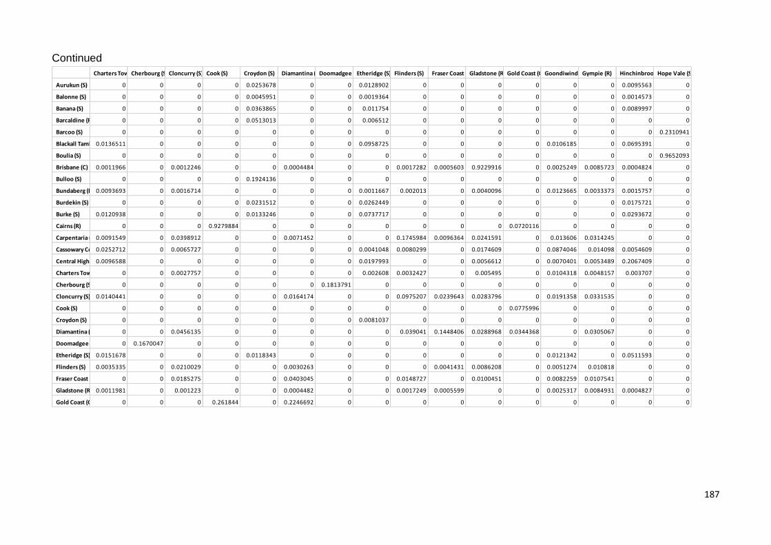
187

Continued

Charters Towers (R) Cherbourg (S) Cloncurry (S) Cook (S) Croydon (S) Diamantina (S) Doomadgee (S) Etheridge (S) Flinders (S) Fraser Coast (R) Gladstone (R) Gold Coast (C) Goondiwindi (R) Gympie (R) Hinchinbrook (S) Hope Vale (S)

Aurukun (S) 0 0 0 0 0.0253678 0 0 0.0128902 0 0 0 0 0 0 0.0095563 0

Balonne (S) 0 0 0 0 0.0045951 0 0 0.0019364 0 0 0 0 0 0 0.0014573 0

Banana (S) 0 0 0 0 0.0363865 0 0 0.011754 0 0 0 0 0 0 0.0089997 0

Barcaldine (R) 0 0 0 0 0.0513013 0 0 0.006512 0 0 0 0 0 0 0 0

Barcoo (S) 0 0 0 0 0 0 0 0 0 0 0 0 0 0 0 0.2310941

Blackall Tambo (R)0.0136511 0 0 0 0 0 0 0.0958725 0 0 0 0 0.0106185 0 0.0695391 0

Boulia (S) 0 0 0 0 0 0 0 0 0 0 0 0 0 0 0 0.9652093

Brisbane (C) 0.0011966 0 0.0012246 0 0 0.0004484 0 0 0.0017282 0.0005603 0.9229916 0 0.0025249 0.0085723 0.0004824 0

Bulloo (S) 0 0 0 0 0.1924136 0 0 0 0 0 0 0 0 0 0 0

Bundaberg (R) 0.0093693 0 0.0016714 0 0 0 0 0.0011667 0.002013 0 0.0040096 0 0.0123665 0.0033373 0.0015757 0

Burdekin (S) 0 0 0 0 0.0231512 0 0 0.0262449 0 0 0 0 0 0 0.0175721 0

Burke (S) 0.0120938 0 0 0 0.0133246 0 0 0.0737717 0 0 0 0 0 0 0.0293672 0

Cairns (R) 0 0 0 0.9279884 0 0 0 0 0 0 0 0.0720116 0 0 0 0

Carpentaria (S)0.0091549 0 0.0398912 0 0 0.0071452 0 0 0.1745984 0.0096364 0.0241591 0 0.013606 0.0314245 0 0

Cassowary Coast (R)0.0252712 0 0.0065727 0 0 0 0 0.0041048 0.0080299 0 0.0174609 0 0.0874046 0.014098 0.0054609 0

Central Highlands (R)0.0096588 0 0 0 0 0 0 0.0197993 0 0 0.0056612 0 0.0070401 0.0053489 0.2067409 0

Charters Towers (R) 0 0 0.0027757 0 0 0 0 0.002608 0.0032427 0 0.005495 0 0.0104318 0.0048157 0.003707 0

Cherbourg (S) 0 0 0 0 0 0 0.1813791 0 0 0 0 0 0 0 0 0

Cloncurry (S) 0.0140441 0 0 0 0 0.0164174 0 0 0.0975207 0.0239643 0.0283796 0 0.0191358 0.0331535 0 0

Cook (S) 0 0 0 0 0 0 0 0 0 0 0 0.0775996 0 0 0 0

Croydon (S) 0 0 0 0 0 0 0 0.0081037 0 0 0 0 0 0 0 0

Diamantina (S) 0 0 0.0456135 0 0 0 0 0 0.039041 0.1448406 0.0288968 0.0344368 0 0.0305067 0 0

Doomadgee (S) 0 0.1670047 0 0 0 0 0 0 0 0 0 0 0 0 0 0

Etheridge (S) 0.0151678 0 0 0 0.0118343 0 0 0 0 0 0 0 0.0121342 0 0.0511593 0

Flinders (S) 0.0035335 0 0.0210029 0 0 0.0030263 0 0 0 0.0041431 0.0086208 0 0.0051274 0.010818 0 0

Fraser Coast (R) 0 0 0.0185275 0 0 0.0403045 0 0 0.0148727 0 0.0100451 0 0.0082259 0.0107541 0 0

Gladstone (R) 0.0011981 0 0.001223 0 0 0.0004482 0 0 0.0017249 0.0005599 0 0 0.0025317 0.0084931 0.0004827 0

Gold Coast (C) 0 0 0 0.261844 0 0.2246692 0 0 0 0 0 0 0 0 0 0

188

Continued

Hope Vale (S) Ipswich (C) Isaac (R) Kowanyama (S) Lockhart River (S) Lockyer Valley (R) Logan (C) Longreach (R) Mackay (R) McKinlay (S) Mapoon (S) Maranoa (R) Moreton Bay (R) Mornington (S) Mount Isa (C) Murweh (S) Napranum (S)

Aurukun (S) 0 0.0182594 0 0.0296191 0 0 0 0 0.0095054 0 0.0105742 0 0.2198699 0.03165 0.0100926 0

Balonne (S) 0 0.0026788 0 0.0041405 0 0 0 0 0.0015864 0 0.0016051 0 0.8614781 0.0043874 0.0015353 0

Banana (S) 0 0.0158401 0 0.0232974 0 0 0 0 0.0110168 0 0.0098596 0 0.1648439 0.0244864 0.0094549 0

Barcaldine (R) 0 0.0083458 0 0.0112673 0 0 0 0 0.008562 0 0 0 0.0311652 0.0116894 0 0

Barcoo (S) 0 0 0.0619258 0 0 0 0 0 0.0787587 0 0 0 0 0 0 0

Blackall Tambo (R)0.0117671 0.0319048 0 0.0197634 0 0 0 0.0108292 0 0 0.1943302 0 0.011666 0.0190169 0.1077274 0

Boulia (S) 0 0 0.0031857 0 0 0 0 0 0.0022245 0.0021199 0 0 0 0 0 0

Brisbane (C) 0.0016971 0 0 0 0.0027487 0.0148383 0.0059131 0.0023012 0 0 0.0004411 0.0091683 0 0 0.0004587 0

Bulloo (S) 0 0.0122606 0 0.0154961 0 0 0 0 0.0207731 0 0 0 0.0298768 0.0159297 0 0

Bundaberg (R) 0.6386504 0 0 0 0.0024685 0.0045227 0.0031053 0.0155197 0 0 0.0013938 0.0033738 0 0 0.0014698 0

Burdekin (S) 0 0.0449407 0 0.1306072 0 0 0 0 0 0 0.0200365 0 0.0527329 0.1625709 0.0188521 0

Burke (S) 0 0.268775 0 0.0509489 0 0 0 0 0 0 0.0378459 0 0.0205591 0.0470186 0.0335117 0

Cairns (R) 0 0 0 0 0 0 0 0 0 0 0 0 0 0 0 0

Carpentaria (S)0.0112109 0 0 0 0.0852263 0.0213757 0.0362869 0.0130503 0 0 0 0.0308274 0 0 0 0

Cassowary Coast (R)0.0911287 0 0 0 0.0100392 0.0201708 0.0129838 0.1433994 0 0 0.0048629 0.0142751 0 0 0.0051138 0

Central Highlands (R)0.0079922 0.0112358 0 0.0080357 0 0.0058537 0.0052206 0.0072114 0 0 0.0457979 0.005368 0.0052885 0.0078064 0.0703216 0

Charters Towers (R)0.0186083 0.0020865 0 0 0.0038234 0.0059693 0.0045642 0.0114331 0 0 0.0032044 0.0048543 0 0 0.0034116 0

Cherbourg (S) 0 0 0.0400903 0 0 0 0 0 0 0.0999236 0 0 0 0 0 0.4729056

Cloncurry (S) 0.0165063 0 0 0 0.051251 0.0262507 0.0358399 0.0185469 0 0 0 0.0327982 0 0 0 0

Cook (S) 0 0 0 0 0 0 0 0 0 0 0 0 0 0 0 0

Croydon (S) 0 0.0100665 0 0.0129557 0 0 0 0 0.0144128 0 0 0 0.0271888 0.0133509 0 0

Diamantina (S) 0 0 0 0 0.0345469 0 0.0312833 0 0 0 0 0.0303977 0 0 0 0

Doomadgee (S) 0 0 0.0473872 0 0 0 0 0 0 0.204869 0 0 0 0 0 0.27091

Etheridge (S) 0.0133033 0.0606957 0 0.0315999 0 0 0 0.0123505 0 0 0.0814893 0 0.0168593 0.0301111 0.0643888 0

Flinders (S) 0.0042793 0 0 0 0.0232641 0.007736 0.0122038 0.0049325 0 0 0 0.0106433 0 0 0 0

Fraser Coast (R) 0 0 0 0 0.0126245 0.0096855 0.0111033 0.0080832 0 0 0 0.0107054 0 0 0 0

Gladstone (R) 0.0017002 0 0 0 0.0027405 0.0150801 0.0058752 0.0023068 0 0 0.0004413 0.0090777 0 0 0.0004589 0

Gold Coast (C) 0 0 0 0 0 0 0 0 0 0 0 0 0 0 0 0

189

Continued

Napranum (S) North Burnett (R) Northern Peninsula Area (R) Palm Island (S) Paroo (S) Pormpuraaw (S) Quilpie (S) Redland (C) Richmond (S) Rockhampton (R) Scenic Rim (R) Somerset (R) South Burnett (R) Southern Downs (R) Sunshine Coast (R) Tablelands (R) Toowoomba (R) Torres (S)

Aurukun (S) 0.024913 0.0089628 0 0.0239101 0.0152608 0 0 0.0402582 0 0 0 0.0088801 0 0 0 0 0

Balonne (S) 0.003552 0.0014919 0 0.0042973 0.0026218 0 0 0.0079272 0 0 0 0.0013583 0 0 0 0 0

Banana (S) 0.0203836 0.0103202 0 0.0335629 0.0190115 0 0 0.0743196 0 0 0 0 0 0 0 0 0

Barcaldine (R) 0.0101848 0.007923 0 0.0433888 0.0172092 0 0 0.4822768 0 0 0 0 0 0 0 0 0

Barcoo (S) 0 0.0853974 0.0848845 0 0 0 0 0 0 0 0 0 0 0 0 0 0

Blackall Tambo (R)0.0223453 0 0 0 0 0.0135903 0.0116297 0.0095858 0 0 0.0186736 0.0461141 0 0 0.0115491 0.0142001 0

Boulia (S) 0 0.0023617 0.0050427 0 0 0 0 0 0 0 0 0 0 0 0 0 0

Brisbane (C) 0 0 0 0 0 0.0012065 0.0017601 0 0.0008062 0.0027574 0.0008002 0.000521 0.0005682 0 0.0018001 0.0011171 0.001622

Bulloo (S) 0.0143466 0.0187608 0 0.3078256 0.0626163 0 0 0.0587588 0 0 0 0 0 0 0 0 0

Bundaberg (R) 0 0 0 0 0 0.0096343 0.1344892 0 0.0012835 0.0024715 0.0035286 0.001757 0 0 0.0779982 0.0075685 0.0019496

Burdekin (S) 0.082726 0 0 0.0222894 0.0163039 0 0 0.0302452 0 0 0 0.016014 0 0 0 0 0

Burke (S) 0.0675785 0 0 0.0130091 0 0.0120544 0 0.0156232 0 0 0.0150578 0.0249463 0 0 0 0.0124459 0

Cairns (R) 0 0 0 0 0 0 0 0 0 0 0 0 0 0 0 0 0

Carpentaria (S) 0 0 0 0 0 0.009202 0.0114307 0 0.0168027 0.0845554 0.0069986 0 0.0098277 0.0060091 0.0115663 0.0087666 0.1135401

Cassowary Coast (R) 0 0 0 0 0 0.0257915 0.117291 0 0.0049673 0.0100527 0.011414 0.0060492 0.0038224 0 0.1416147 0.0215164 0.007756

Central Highlands (R)0.0087964 0 0 0 0 0.0096029 0.0078759 0 0 0 0.0148664 0.1161536 0 0 0.0078079 0.0101709 0

Charters Towers (R) 0 0 0 0 0 0.6667009 0.0171411 0 0.0022091 0.0038271 0.0110769 0.0042321 0 0 0.016369 0.0770602 0.0031581

Cherbourg (S) 0 0 0.0278673 0 0 0 0 0 0 0 0 0 0 0 0 0 0

Cloncurry (S) 0 0 0 0 0 0.0141029 0.0167578 0 0.0547556 0.0511217 0.0112301 0 0.0245957 0.0133439 0.0169119 0.0135559 0.1159926

Cook (S) 0 0 0 0 0 0 0 0 0 0 0 0 0 0 0 0 0

Croydon (S) 0.0119171 0.0131406 0 0.3945128 0.0363165 0 0 0.0650272 0 0 0 0 0 0 0 0 0

Diamantina (S) 0 0 0 0 0 0 0 0 0.0651464 0.0345257 0 0 0.1371805 0.1980331 0 0 0.0399579

Doomadgee (S) 0 0 0.0303167 0 0 0 0 0 0 0 0 0 0 0 0 0 0

Etheridge (S) 0.0369829 0 0 0 0 0.0151087 0.0131648 0.013519 0 0 0.0198386 0.0395229 0 0 0.0130833 0.0156991 0

Flinders (S) 0 0 0 0 0 0.0035508 0.004358 0 0.0075523 0.0231407 0.0027334 0 0.0042302 0.002528 0.0044065 0.0033909 0.1318857

Fraser Coast (R) 0 0 0 0 0 0 0 0 0.0329471 0.0126143 0 0 0.7217939 0.0232786 0 0 0.0153551

Gladstone (R) 0 0 0 0 0 0.0012081 0.0017634 0 0.0008055 0.0027491 0.0008008 0.0005213 0.0005678 0 0.0018036 0.0011184 0.0016191

Gold Coast (C) 0 0 0 0 0 0 0 0 0 0 0 0 0 0.2719619 0 0 0

190

Continued

Torres Strait Island (R) Townsville (C) Weipa (T) Western Downs (R) Whitsunday (R) Winton (S) Woorabinda (S) Wujal Wujal (S) Yarrabah (S)

Aurukun (S) 0 0 0.0466918 0.0091327 0 0 0 0 0

Balonne (S) 0 0 0.0095535 0.0013953 0 0 0 0 0

Banana (S) 0.0091128 0 0.0983995 0 0 0 0 0 0

Barcaldine (R) 0.0068515 0 0.1401365 0 0 0 0 0 0

Barcoo (S) 0.1037169 0 0 0 0 0 0.0632519 0 0.0577672

Blackall Tambo (R) 0 0 0.009883 0.0531057 0 0.0128868 0 0 0

Boulia (S) 0.0027124 0 0 0 0 0 0.0032793 0.0021521 0.0029013

Brisbane (C) 0 0.0017037 0 0.0005052 0 0.0013434 0 0 0

Bulloo (S) 0.0155952 0 0.0505211 0 0 0 0 0 0

Bundaberg (R) 0 0.0019987 0 0.0016814 0 0.0147543 0 0 0

Burdekin (S) 0 0 0.0325893 0.0165889 0 0 0 0 0

Burke (S) 0 0 0.0162826 0.0265057 0 0.0115907 0 0 0

Cairns (R) 0 0 0 0 0 0 0 0 0

Carpentaria (S) 0 0.156158 0 0 0 0.0098221 0 0 0

Cassowary Coast (R) 0 0.0079681 0 0.0058048 0 0.034509 0 0 0

Central Highlands (R) 0 0 0 0.2981381 0 0.0089662 0 0 0

Charters Towers (R) 0 0.0032237 0 0.0040101 0 0.0502368 0 0 0

Cherbourg (S) 0 0 0 0 0 0 0.0387721 0.0936729 0.0453892

Cloncurry (S) 0 0.1010545 0 0 0 0.0148655 0 0 0

Cook (S) 0 0 0 0 0 0 0 0 0

Croydon (S) 0.0110896 0 0.0526648 0 0 0 0 0 0

Diamantina (S) 0 0.0392387 0 0 0 0 0 0 0

Doomadgee (S) 0 0 0 0 0 0 0.0454054 0.1783661 0.055741

Etheridge (S) 0 0 0.0139864 0.0433791 0 0.0144192 0 0 0

Flinders (S) 0 0.6006052 0 0 0 0.0037774 0 0 0

Fraser Coast (R) 0 0.014976 0 0 0 0 0 0 0

Gladstone (R) 0 0.0017005 0 0.0005055 0 0.0013453 0 0 0

Gold Coast (C) 0 0 0 0 0 0 0 0 0

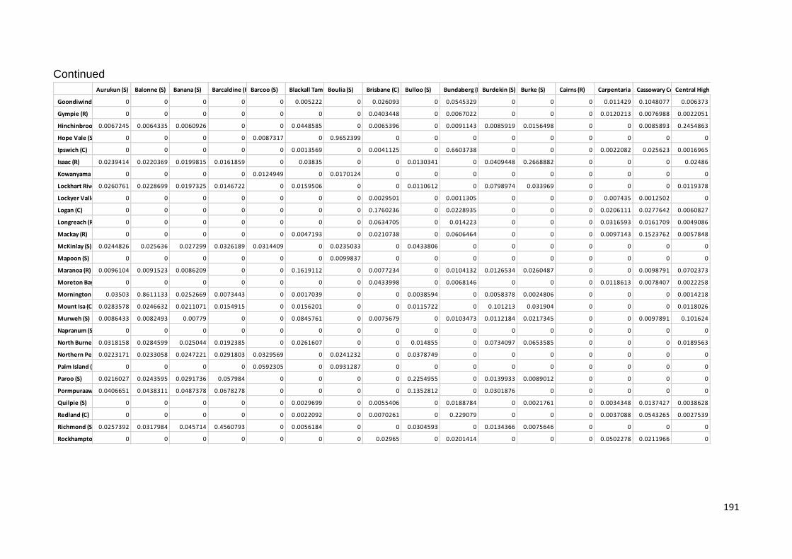
191

Continued


Goondiwindi (R) 0 0 0 0 0 0.005222 0 0.026093 0 0.0545329 0 0 0 0.011429 0.1048077 0.006373

Gympie (R) 0 0 0 0 0 0 0 0.0403448 0 0.0067022 0 0 0 0.0120213 0.0076988 0.0022051

Hinchinbrook (S)0.0067245 0.0064335 0.0060926 0 0 0.0448585 0 0.0065396 0 0.0091143 0.0085919 0.0156498 0 0 0.0085893 0.2454863

Hope Vale (S) 0 0 0 0 0.0087317 0 0.9652399 0 0 0 0 0 0 0 0 0

Ipswich (C) 0 0 0 0 0 0.0013569 0 0.0041125 0 0.6603738 0 0 0 0.0022082 0.025623 0.0016965

Isaac (R) 0.0239414 0.0220369 0.0199815 0.0161859 0 0.03835 0 0 0.0130341 0 0.0409448 0.2668882 0 0 0 0.02486

Kowanyama (S) 0 0 0 0 0.0124949 0 0.0170124 0 0 0 0 0 0 0 0 0

Lockhart River (S)0.0260761 0.0228699 0.0197325 0.0146722 0 0.0159506 0 0 0.0110612 0 0.0798974 0.033969 0 0 0 0.0119378

Lockyer Valley (R) 0 0 0 0 0 0 0 0.0029501 0 0.0011305 0 0 0 0.007435 0.0012502 0

Logan (C) 0 0 0 0 0 0 0 0.1760236 0 0.0228935 0 0 0 0.0206111 0.0277642 0.0060827

Longreach (R) 0 0 0 0 0 0 0 0.0634705 0 0.014223 0 0 0 0.0316593 0.0161709 0.0049086

Mackay (R) 0 0 0 0 0 0.0047193 0 0.0210738 0 0.0606464 0 0 0 0.0097143 0.1523762 0.0057848

McKinlay (S) 0.0244826 0.025636 0.027299 0.0326189 0.0314409 0 0.0235033 0 0.0433806 0 0 0 0 0 0 0

Mapoon (S) 0 0 0 0 0 0 0.0099837 0 0 0 0 0 0 0 0 0

Maranoa (R) 0.0096104 0.0091523 0.0086209 0 0 0.1619112 0 0.0077234 0 0.0104132 0.0126534 0.0260487 0 0 0.0098791 0.0702373

Moreton Bay (R) 0 0 0 0 0 0 0 0.0433998 0 0.0068146 0 0 0 0.0118613 0.0078407 0.0022258

Mornington (S) 0.03503 0.8611133 0.0252669 0.0073443 0 0.0017039 0 0 0.0038594 0 0.0058378 0.0024806 0 0 0 0.0014218

Mount Isa (C) 0.0283578 0.0246632 0.0211071 0.0154915 0 0.0156201 0 0 0.0115722 0 0.101213 0.031904 0 0 0 0.0118026

Murweh (S) 0.0086433 0.0082493 0.00779 0 0 0.0845761 0 0.0075679 0 0.0103473 0.0112184 0.0217345 0 0 0.0097891 0.101624

Napranum (S) 0 0 0 0 0 0 0 0 0 0 0 0 0 0 0 0

North Burnett (R)0.0318158 0.0284599 0.025044 0.0192385 0 0.0261607 0 0 0.014855 0 0.0734097 0.0653585 0 0 0 0.0189563

Northern Peninsula Area (R)0.0223171 0.0233058 0.0247221 0.0291803 0.0329569 0 0.0241232 0 0.0378749 0 0 0 0 0 0 0

Palm Island (S) 0 0 0 0 0.0592305 0 0.0931287 0 0 0 0 0 0 0 0 0

Paroo (S) 0.0216027 0.0243595 0.0291736 0.057984 0 0 0 0 0.2254955 0 0.0139933 0.0089012 0 0 0 0

Pormpuraaw (S)0.0406651 0.0438311 0.0487378 0.0678278 0 0 0 0 0.1352812 0 0.0301876 0 0 0 0 0

Quilpie (S) 0 0 0 0 0 0.0029699 0 0.0055406 0 0.0188784 0 0.0021761 0 0.0034348 0.0137427 0.0038628

Redland (C) 0 0 0 0 0 0.0022092 0 0.0070261 0 0.229079 0 0 0 0.0037088 0.0543265 0.0027539

Richmond (S) 0.0257392 0.0317984 0.045714 0.4560793 0 0.0056184 0 0 0.0304593 0 0.0134366 0.0075646 0 0 0 0

Rockhampton (R) 0 0 0 0 0 0 0 0.02965 0 0.0201414 0 0 0 0.0502278 0.0211966 0

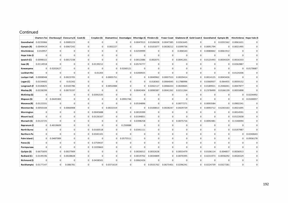
192

Continued


Goondiwindi (R)0.0235066 0 0.0085223 0 0 0 0 0.0047013 0.0106028 0.0047385 0.0261645 0 0 0.0201562 0.0061631 0

Gympie (R) 0.0049419 0 0.0067242 0 0 0.002227 0 0 0.0101877 0.0028212 0.0399736 0 0.0091794 0 0.0021495 0

Hinchinbrook (S)0.010957 0 0 0 0 0 0 0.0259999 0 0 0.006543 0 0.0080842 0.0061912 0 0

Hope Vale (S) 0 0 0 0 0 0 0 0 0 0 0 0 0 0 0 0

Ipswich (C) 0.0098322 0 0.0017238 0 0 0 0 0.0012086 0.002075 0 0.0041201 0 0.0125443 0.0034329 0.0016333 0

Isaac (R) 0.0114918 0 0 0 0.0139212 0 0 0.0574777 0 0 0 0 0 0 0.0262887 0

Kowanyama (S) 0 0.0202627 0 0 0 0 0.0260121 0 0 0 0 0 0 0 0 0.0170687

Lockhart River (S) 0 0 0 0 0.01203 0 0 0.0200925 0 0 0 0 0 0 0.0124206 0

Lockyer Valley (R)0.0008948 0 0.0023705 0 0 0.0005751 0 0 0.0049962 0.0007553 0.0029414 0 0.0014125 0.0043426 0 0

Logan (C) 0.0154402 0 0.01342 0 0 0 0 0 0.018363 0.0064045 0.1788996 0 0.0360937 0.064455 0.0059152 0

Longreach (R) 0.0106825 0 0.0165786 0 0 0.0052084 0 0 0.0262117 0.0066433 0.0630665 0 0.0189921 0.2046041 0.0047877 0

Mackay (R) 0.0228299 0 0.0073197 0 0 0 0 0.0042404 0.0090387 0.0041262 0.0211264 0 0.2378499 0.0166139 0.0055898 0

McKinlay (S) 0 0 0 0 0.0391535 0 0 0 0 0 0 0 0 0 0 0.0234492

Mapoon (S) 0 0.0445383 0 0 0 0 0.0991746 0 0 0 0 0 0 0 0 0.0100057

Maranoa (R) 0.0122331 0 0 0 0 0 0 0.0534896 0 0 0.0077271 0 0.0093584 0 0.0902241 0

Moreton Bay (R)0.0050104 0 0.0066908 0 0 0.0022319 0 0 0.0100813 0.0028247 0.0429729 0 0.0093712 0.6243163 0.0021695 0

Mornington (S) 0 0 0 0 0.0045688 0 0 0.0019399 0 0 0 0 0 0 0.0014591 0

Mount Isa (C) 0 0 0 0 0.0126167 0 0 0.0194851 0 0 0 0 0 0 0.0122658 0

Murweh (S) 0.0122725 0 0 0 0 0 0 0.0398258 0 0 0.0075716 0 0.0092481 0 0.1540094 0

Napranum (S) 0 0.4019609 0 0 0 0 0.250088 0 0 0 0 0 0 0 0 0

North Burnett (R) 0 0 0 0 0.0160518 0 0 0.0341111 0 0 0 0 0 0 0.0197987 0

Northern Peninsula Area (R)0 0 0 0 0.0345101 0 0 0 0 0 0 0 0 0 0 0.0240643

Palm Island (S) 0 0.0487089 0 0 0 0 0.0575511 0 0 0 0 0 0 0 0 0.0936178

Paroo (S) 0 0 0 0 0.3759437 0 0 0 0 0 0 0 0 0 0 0

Pormpuraaw (S) 0 0 0 0 0.1020663 0 0 0 0 0 0 0 0 0 0 0

Quilpie (S) 0.6675693 0 0.0027909 0 0 0 0 0.0026012 0.0032628 0 0.0055479 0 0.0106114 0.004857 0.0036913 0

Redland (C) 0.0149196 0 0.0028828 0 0 0 0 0.0019702 0.0034809 0 0.0070395 0 0.0231973 0.0058292 0.0026529 0

Richmond (S) 0 0 0 0 0.0438501 0 0 0.0062426 0 0 0 0 0 0 0 0

Rockhampton (R)0.0177147 0 0.086781 0 0 0.0371619 0 0 0.0555762 0.0675401 0.0296241 0 0.0224739 0.0327281 0 0

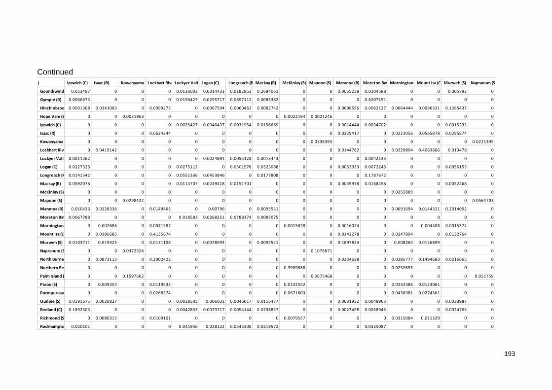
193

Continued


Goondiwindi (R)0.053497 0 0 0 0.0136003 0.0314433 0.0182852 0.2684061 0 0 0.0055238 0.0204588 0 0 0.005793 0

Gympie (R) 0.0066673 0 0 0 0.0190427 0.0255717 0.0897112 0.0085382 0 0 0 0.6207151 0 0 0 0

Hinchinbrook (S)0.0091368 0.0141083 0 0.0099275 0 0.0067594 0.0060463 0.0082742 0 0 0.0698556 0.0062127 0.0064444 0.0096331 0.1265437 0

Hope Vale (S) 0 0 0.0031963 0 0 0 0 0 0.0022194 0.0021246 0 0 0 0 0 0

Ipswich (C) 0 0 0 0 0.0025427 0.0046437 0.0031954 0.0156669 0 0 0.0014444 0.0034702 0 0 0.0015233 0

Isaac (R) 0 0 0 0.0624244 0 0 0 0 0 0 0.0329417 0 0.0221056 0.0565878 0.0295874 0

Kowanyama (S) 0 0 0 0 0 0 0 0 0 0.0338393 0 0 0 0 0 0.0221395

Lockhart River (S) 0 0.0419142 0 0 0 0 0 0 0 0 0.0144782 0 0.0229804 0.4063666 0.013478 0

Lockyer Valley (R)0.0011262 0 0 0 0 0.0024891 0.0055128 0.0013443 0 0 0 0.0042133 0 0 0 0

Logan (C) 0.0227325 0 0 0 0.0275112 0 0.0501578 0.0323088 0 0 0.0053933 0.0672245 0 0 0.0056153 0

Longreach (R) 0.0141542 0 0 0 0.0551336 0.0453846 0 0.0177808 0 0 0 0.1787672 0 0 0 0

Mackay (R) 0.0592076 0 0 0 0.0114707 0.0249418 0.0151701 0 0 0 0.0049978 0.0168456 0 0 0.0052468 0

McKinlay (S) 0 0 0 0 0 0 0 0 0 0 0 0 0.0255889 0 0 0

Mapoon (S) 0 0 0.0298422 0 0 0 0 0 0 0 0 0 0 0 0 0.0564703

Maranoa (R) 0.010436 0.0228336 0 0.0149463 0 0.00796 0 0.0095551 0 0 0 0 0.0091694 0.0144321 0.2014052 0

Moreton Bay (R)0.0067788 0 0 0 0.018583 0.0268251 0.0788374 0.0087075 0 0 0 0 0 0 0 0

Mornington (S) 0 0.002686 0 0.0041587 0 0 0 0 0.0015828 0 0.0016074 0 0 0.004408 0.0015374 0

Mount Isa (C) 0 0.0386685 0 0.4135674 0 0 0 0 0 0 0.0142278 0 0.0247894 0 0.0132764 0

Murweh (S) 0.0103711 0.019325 0 0.0131108 0 0.0078093 0 0.0094521 0 0 0.1897824 0 0.008264 0.0126899 0 0

Napranum (S) 0 0 0.0372324 0 0 0 0 0 0 0.1076871 0 0 0 0 0 0

North Burnett (R) 0 0.0873113 0 0.2002423 0 0 0 0 0 0 0.0234628 0 0.0285777 0.1494683 0.0216665 0

Northern Peninsula Area (R)0 0 0 0 0 0 0 0 0.3909888 0 0 0 0.0232655 0 0 0

Palm Island (S) 0 0 0.1597602 0 0 0 0 0 0 0.0675468 0 0 0 0 0 0.051759

Paroo (S) 0 0.009354 0 0.0119533 0 0 0 0 0.0142552 0 0 0 0.0242386 0.0123061 0 0

Pormpuraaw (S) 0 0 0 0.0268374 0 0 0 0 0.0671603 0 0 0 0.0436981 0.0274361 0 0

Quilpie (S) 0.0191675 0.0020827 0 0 0.0038505 0.006031 0.0046017 0.0116477 0 0 0.0031932 0.0048963 0 0 0.0033987 0

Redland (C) 0.1892303 0 0 0 0.0042833 0.0079717 0.0054144 0.0298837 0 0 0.0023498 0.0058945 0 0 0.0024765 0

Richmond (S) 0 0.0080315 0 0.0109101 0 0 0 0 0.0079557 0 0 0 0.0315084 0.011329 0 0

Rockhampton (R)0.020101 0 0 0 0.041956 0.028122 0.0343308 0.0219572 0 0 0 0.0325087 0 0 0 0

194

Continued


Goondiwindi (R) 0 0 0 0 0 0.0238802 0.060055 0 0.0063152 0.0136208 0.0121058 0.0067842 0.0047931 0 0.0648081 0.0207038 0.010206

Gympie (R) 0 0 0 0 0 0.0049778 0.0068727 0 0.0041883 0.0191313 0.0034444 0.0023116 0.0028639 0 0.0070018 0.0046512 0.0094154

Hinchinbrook (S)0.0109091 0 0 0 0 0.0108964 0.0090088 0 0 0 0.0164683 0.0883079 0 0 0.0089338 0.0115108 0

Hope Vale (S) 0 0.002356 0.0050693 0 0 0 0 0 0 0 0 0 0 0 0 0 0

Ipswich (C) 0 0 0 0 0 0.0101146 0.1148734 0 0.0013245 0.0025457 0.0036689 0.0018218 0 0 0.0718734 0.0079198 0.0020097

Isaac (R) 0.0896433 0 0 0.0135748 0 0.0114559 0 0.0164709 0 0 0.0141589 0.0226673 0 0 0 0.0118116 0

Kowanyama (S) 0 0 0.0461968 0 0 0 0 0 0 0 0 0 0 0 0 0 0

Lockhart River (S)0.1380415 0 0 0.0116475 0.0088668 0 0 0.0150232 0 0 0.0077492 0.0111654 0 0 0 0 0

Lockyer Valley (R) 0 0 0 0 0 0.0008999 0.0011516 0 0.0012244 0.9370154 0.0006652 0 0.0007687 0.0004897 0.0011675 0.0008525 0.004247

Logan (C) 0 0 0 0 0 0.0155797 0.0236901 0 0.0090711 0.0275845 0.0100333 0.0064055 0.0064916 0 0.0243026 0.0143302 0.0173455

Longreach (R) 0 0 0 0 0 0.0107561 0.0145592 0 0.0100201 0.0554599 0.0075652 0.0051396 0.0067471 0 0.0148128 0.0100851 0.0239917

Mackay (R) 0 0 0 0 0 0.0232282 0.0685578 0 0.0054677 0.0114872 0.0112343 0.0061677 0.004173 0 0.075711 0.0198803 0.0087128

McKinlay (S) 0 0.4044446 0 0.0406382 0.0649168 0 0 0.0320499 0 0 0 0 0 0 0 0 0

Mapoon (S) 0 0 0.0172249 0 0 0 0 0 0 0 0 0 0 0 0 0 0

Maranoa (R) 0.0166976 0 0 0 0 0.0121746 0.0103064 0 0 0 0.0172124 0.0503751 0 0 0.0102304 0.0127638 0

Moreton Bay (R) 0 0 0 0 0 0.0050472 0.00699 0 0.0041844 0.018667 0.0034837 0.0023337 0.0028673 0 0.0071227 0.0047135 0.0093285

Mornington (S)0.0035652 0.0014887 0 0.0042742 0.0026127 0 0 0.0078516 0 0 0 0.0013599 0 0 0 0 0

Mount Isa (C) 0.1048652 0 0 0.0122037 0.0092252 0 0 0.0158763 0 0 0.0077389 0.0110594 0 0 0 0 0

Murweh (S) 0.0145294 0 0 0 0 0.0122101 0.0102354 0 0 0 0.0177347 0.0633006 0 0 0.0101559 0.012841 0

Napranum (S) 0 0 0.0251699 0 0 0 0 0 0 0 0 0 0 0 0 0 0

North Burnett (R) 0 0 0 0.0155811 0.0120859 0 0 0.0196536 0 0 0.0119095 0.0176218 0 0 0 0 0

Northern Peninsula Area (R)0 0 0 0.0356991 0.0540772 0 0 0.0287086 0 0 0 0 0 0 0 0 0

Palm Island (S) 0 0 0 0 0 0 0 0 0 0 0 0 0 0 0 0 0

Paroo (S) 0.0110232 0.0129536 0 0 0.0381158 0 0 0.0531979 0 0 0 0 0 0 0 0 0

Pormpuraaw (S)0.0252176 0.0578714 0 0.1124144 0 0 0 0.0654909 0 0 0 0 0 0 0 0 0

Quilpie (S) 0 0 0 0 0 0 0.0176164 0 0.0022193 0.0038542 0.01091 0.0042109 0 0 0.0168029 0.0691661 0.0031772

Redland (C) 0 0 0 0 0 0.0153133 0 0 0.0022073 0.0042886 0.0058566 0.0029542 0 0 0.3162939 0.0122048 0.0033696

Richmond (S) 0.0098393 0.0073716 0 0.0376451 0.0157137 0 0 0 0 0 0 0 0 0 0 0 0

Rockhampton (R) 0 0 0 0 0 0.0177736 0.0203354 0 0 0.0419012 0 0 0.0707705 0.027963 0.0204783 0.017221 0.058952

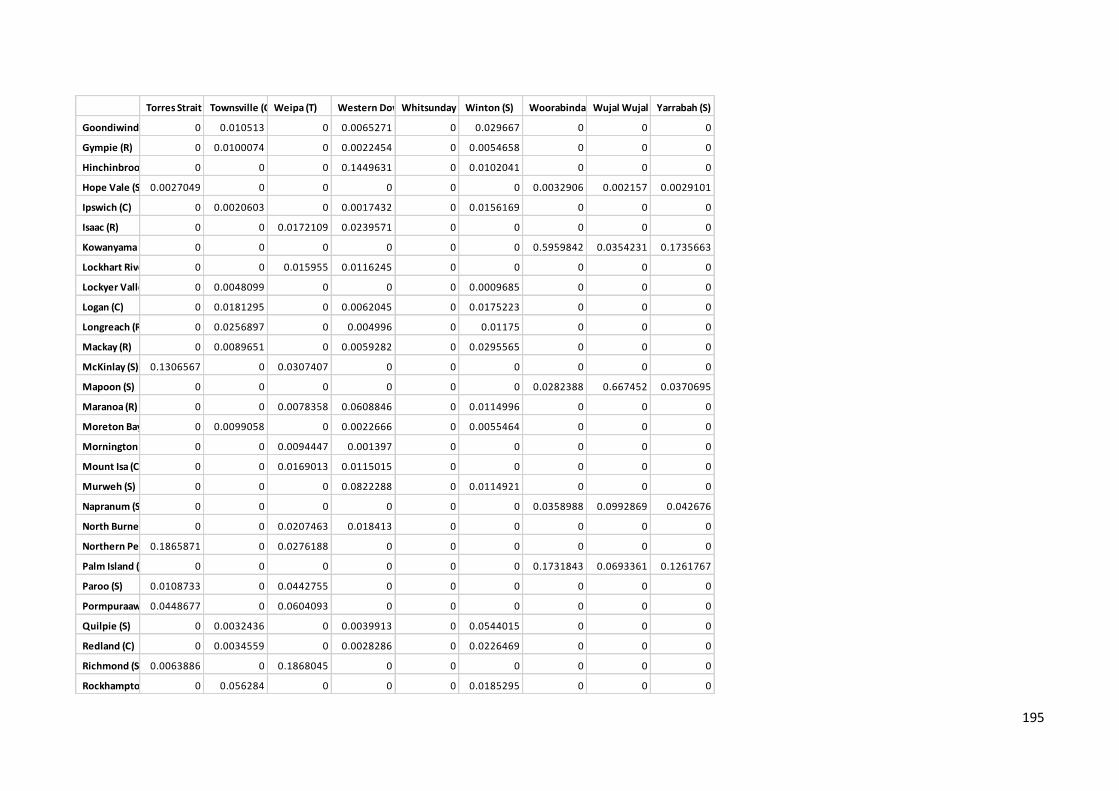
195


Goondiwindi (R) 0 0.010513 0 0.0065271 0 0.029667 0 0 0

Gympie (R) 0 0.0100074 0 0.0022454 0 0.0054658 0 0 0

Hinchinbrook (S) 0 0 0 0.1449631 0 0.0102041 0 0 0

Hope Vale (S) 0.0027049 0 0 0 0 0 0.0032906 0.002157 0.0029101

Ipswich (C) 0 0.0020603 0 0.0017432 0 0.0156169 0 0 0

Isaac (R) 0 0 0.0172109 0.0239571 0 0 0 0 0

Kowanyama (S) 0 0 0 0 0 0 0.5959842 0.0354231 0.1735663

Lockhart River (S) 0 0 0.015955 0.0116245 0 0 0 0 0

Lockyer Valley (R) 0 0.0048099 0 0 0 0.0009685 0 0 0

Logan (C) 0 0.0181295 0 0.0062045 0 0.0175223 0 0 0

Longreach (R) 0 0.0256897 0 0.004996 0 0.01175 0 0 0

Mackay (R) 0 0.0089651 0 0.0059282 0 0.0295565 0 0 0

McKinlay (S) 0.1306567 0 0.0307407 0 0 0 0 0 0

Mapoon (S) 0 0 0 0 0 0 0.0282388 0.667452 0.0370695

Maranoa (R) 0 0 0.0078358 0.0608846 0 0.0114996 0 0 0

Moreton Bay (R) 0 0.0099058 0 0.0022666 0 0.0055464 0 0 0

Mornington (S) 0 0 0.0094447 0.001397 0 0 0 0 0

Mount Isa (C) 0 0 0.0169013 0.0115015 0 0 0 0 0

Murweh (S) 0 0 0 0.0822288 0 0.0114921 0 0 0

Napranum (S) 0 0 0 0 0 0 0.0358988 0.0992869 0.042676

North Burnett (R) 0 0 0.0207463 0.018413 0 0 0 0 0

Northern Peninsula Area (R)0.1865871 0 0.0276188 0 0 0 0 0 0

Palm Island (S) 0 0 0 0 0 0 0.1731843 0.0693361 0.1261767

Paroo (S) 0.0108733 0 0.0442755 0 0 0 0 0 0

Pormpuraaw (S)0.0448677 0 0.0604093 0 0 0 0 0 0

Quilpie (S) 0 0.0032436 0 0.0039913 0 0.0544015 0 0 0

Redland (C) 0 0.0034559 0 0.0028286 0 0.0226469 0 0 0

Richmond (S) 0.0063886 0 0.1868045 0 0 0 0 0 0

Rockhampton (R) 0 0.056284 0 0 0 0.0185295 0 0 0

196

Continued


Scenic Rim (R) 0 0 0 0 0 0 0 0.0029595 0 0.0011319 0 0 0 0.0073766 0.0012519 0

Somerset (R) 0 0 0 0 0 0.0225579 0 0.0203124 0 0.038221 0 0.0150267 0 0.0144406 0.0336195 0.0330569

South Burnett (R)0.0073428 0.0070466 0 0 0 0.034956 0 0.0082992 0 0.0119428 0.009201 0.0156216 0 0 0.0111808 0.1620713

Southern Downs (R) 0 0 0 0 0 0 0 0.0100927 0 0 0 0 0 0.0141896 0.0078785 0

Sunshine Coast (R) 0 0 0 0 0 0 0 0 0 0 0 0 0 0.0463471 0 0

Tablelands (R) 0 0 0 0 0 0.0025911 0 0.0084867 0 0.1569094 0 0 0 0.0044323 0.0774679 0.0032244

Toowoomba (R) 0 0 0 0 0 0.0084904 0 0.0140352 0 0.0405771 0 0.0061475 0 0.0089531 0.0313682 0.0111939

Torres (S) 0 0 0 0 0 0 0 0.0151282 0 0.0077589 0 0 0 0.0860748 0.0083936 0

Torres Strait Island (R) 0 0 0.0342827 0.0396288 0.0628605 0 0.0435096 0 0.0494443 0 0 0 0 0 0 0

Townsville (C) 0 0 0 0 0 0 0 0.0082864 0 0.0041481 0 0 0 0.0617336 0.0044967 0

Weipa (T) 0.0428356 0.0549879 0.0868485 0.19016 0 0.0083119 0 0 0.0375789 0 0.0207746 0.0113126 0 0 0 0

Western Downs (R)0.0055927 0.0053609 0 0 0 0.0298131 0 0.00596 0 0.008464 0.0070588 0.0122924 0 0 0.0079458 0.3080838

Whitsunday (R) 0 0 0 0 0 0 0 0 0 0 0 0 0 0 0 0

Winton (S) 0 0 0 0 0 0.0072176 0 0.0158105 0 0.0740967 0 0.0053628 0 0.0093962 0.0471262 0.0092436

Woorabinda (S) 0 0 0 0 0.013299 0 0.0182485 0 0 0 0 0 0 0 0 0

Wujal Wujal (S) 0 0 0 0 0 0 0.0102837 0 0 0 0 0 0 0 0 0

Yarrabah (S) 0 0 0 0 0.0210919 0 0.028037 0 0 0 0 0 0 0 0 0

197

Continued


Scenic Rim (R) 0.0008956 0 0.0023646 0 0 0.0005748 0 0 0.0049698 0.0007547 0.0029507 0 0.0014146 0.0043629 0 0

Somerset (R) 0.0613115 0 0.0122853 0 0 0 0 0.0188805 0.0138841 0 0.02033 0 0.0297363 0.0185782 0.0308393 0

South Burnett (R)0.0146994 0 0 0 0 0 0 0.0236031 0 0 0.0083039 0 0.010457 0.0078237 0.10377 0

Southern Downs (R) 0 0 0.0188282 0 0 0.0377967 0 0 0.015036 0.7146806 0.0100865 0 0.0082388 0.0108092 0 0

Sunshine Coast (R) 0 0 0.0545668 0 0 0.2914712 0 0 0.0479991 0.1231266 0 0.0613544 0 0 0 0

Tablelands (R) 0.016827 0 0.003436 0 0 0 0 0.0023125 0.0041569 0 0.0085033 0 0.0295654 0.0070138 0.0031071 0

Toowoomba (R)0.2111162 0 0.00734 0 0 0 0 0.0073951 0.008525 0 0.0140522 0 0.0251717 0.0124172 0.0106691 0

Torres (S) 0.0064225 0 0.0466217 0 0 0.0057806 0 0 0.2461341 0.0079829 0.0151017 0 0.009211 0.0186587 0 0

Torres Strait Island (R) 0 0 0 0 0.0457372 0 0 0 0 0 0 0 0 0 0 0.0433877

Townsville (C) 0.0034188 0 0.0211809 0 0 0.0029602 0 0 0.5845125 0.0040601 0.0082711 0 0.0049478 0.0103418 0 0

Weipa (T) 0 0 0 0 0.0509589 0 0 0.0092672 0 0 0 0 0 0 0 0

Western Downs (R)0.0103152 0 0 0 0 0 0 0.0191857 0 0 0.0059633 0 0.0074509 0.0056283 0.126156 0

Whitsunday (R) 0 0 0 0 0 0 0 0 0 0 0 0 0 0 0 0

Winton (S) 0.1289208 0 0.0075398 0 0 0 0 0.0063624 0.0088958 0 0.0158335 0 0.0337866 0.0136685 0.0088594 0

Woorabinda (S) 0 0.0204203 0 0 0 0 0.0259722 0 0 0 0 0 0 0 0 0.0183108

Wujal Wujal (S) 0 0.0423638 0 0 0 0 0.0876097 0 0 0 0 0 0 0 0 0.0103067

Yarrabah (S) 0 0.041513 0 0 0 0 0.0553688 0 0 0 0 0 0 0 0 0.0281215

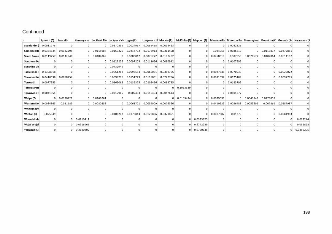
198

Continued


Scenic Rim (R) 0.0011275 0 0 0 0.9370395 0.0024957 0.0055455 0.0013463 0 0 0 0.0042325 0 0 0 0

Somerset (R) 0.0384334 0.0142295 0 0.0115987 0.0157326 0.0214702 0.0178913 0.0311408 0 0 0.024956 0.0186819 0 0.0113817 0.0272881 0

South Burnett (R)0.0119757 0.0142948 0 0.0104869 0 0.0086012 0.0076272 0.0107282 0 0 0.0458318 0.007853 0.0070577 0.0102064 0.0611187 0

Southern Downs (R) 0 0 0 0 0.0127226 0.0097205 0.0111656 0.0080942 0 0 0 0.0107595 0 0 0 0

Sunshine Coast (R) 0 0 0 0 0.0432945 0 0 0 0 0 0 0 0 0 0 0

Tablelands (R) 0.1398318 0 0 0 0.0051282 0.0096584 0.0065061 0.0389765 0 0 0.0027548 0.0070939 0 0 0.0029022 0

Toowoomba (R)0.0410638 0.0058754 0 0 0.0099796 0.0151779 0.0118051 0.0272756 0 0 0.0091597 0.0125109 0 0 0.0097795 0

Torres (S) 0.0077353 0 0 0 0.0369068 0.0136375 0.0208466 0.0088735 0 0 0 0.0183799 0 0 0 0

Torres Strait Island (R) 0 0 0 0 0 0 0 0 0.1983639 0 0 0 0 0 0 0

Townsville (C) 0.0041351 0 0 0 0.0217965 0.007433 0.0116403 0.0047613 0 0 0 0.0101777 0 0 0 0

Weipa (T) 0 0.0120421 0 0.0166261 0 0 0 0 0.0109494 0 0.0079096 0 0.0543848 0.0173055 0 0

Western Downs (R)0.0084863 0.011189 0 0.0080858 0 0.0061701 0.0054909 0.0076366 0 0 0.0410239 0.0056488 0.0053696 0.007861 0.0587987 0

Whitsunday (R) 0 0 0 0 0 0 0 0 0 0 0 0 0 0 0 0

Winton (S) 0.075849 0 0 0 0.0106202 0.0173843 0.0128836 0.0379851 0 0 0.0077302 0.01379 0 0 0.0081983 0

Woorabinda (S) 0 0 0.6210411 0 0 0 0 0 0 0.0333675 0 0 0 0 0 0.022244

Wujal Wujal (S) 0 0 0.0316965 0 0 0 0 0 0 0.6772289 0 0 0 0 0 0.052828

Yarrabah (S) 0 0 0.3140802 0 0 0 0 0 0 0.0760645 0 0 0 0 0 0.0459205

199

Continued


Scenic Rim (R) 0 0 0 0 0 0.0009008 0.0011531 0 0.0012229 0 0.0006657 0 0.0007681 0.0004894 0.0011689 0.0008533 0.004228

Somerset (R) 0.0122886 0 0 0 0 0.0603094 0.0372439 0 0 0.0157437 0 0.0379089 0 0 0.0365668 0.0716041 0.0136022

South Burnett (R)0.0114097 0 0 0 0 0.0146067 0.0117888 0 0 0 0.023788 0 0 0 0.0116797 0.0155536 0

Southern Downs (R) 0 0 0 0 0 0 0 0 0.0341827 0.0127121 0 0 0 0.0223291 0 0 0.0155342

Sunshine Coast (R) 0 0 0 0 0 0 0 0 0.0721496 0.0432719 0 0 0.1192797 0 0 0 0.0489371

Tablelands (R) 0 0 0 0 0 0.0172505 0.3735573 0 0.0026252 0.0051346 0.0067912 0.0034568 0 0 0 0.0138789 0.0040225

Toowoomba (R) 0 0 0 0 0 0.1892427 0.0384153 0 0.0058835 0.0099887 0.0354409 0.0122682 0 0 0.036988 0 0.0083114

Torres (S) 0 0 0 0 0 0.006453 0.007873 0 0.0149507 0.0367403 0.0049976 0 0.0081564 0.00481 0.0079578 0.0061696 0

Torres Strait Island (R) 0 0.2930268 0 0.0470601 0.0658431 0 0 0.0390737 0 0 0 0 0 0 0 0 0

Townsville (C) 0 0 0 0 0 0.0034354 0.0042107 0 0.0074435 0.0216852 0.0026481 0 0.0041461 0.0024706 0.0042572 0.0032815 0.1644669

Weipa (T) 0.0149035 0.010176 0 0.0449574 0.0207982 0 0 0.2680473 0 0 0 0 0 0 0 0 0

Western Downs (R)0.0088293 0 0 0 0 0.0102535 0.0083595 0 0 0 0.0161686 0.1966379 0 0 0.0082854 0.0108814 0

Whitsunday (R) 0 0 0 0 0 0 0 0 0 0 0 0 0 0 0 0 0

Winton (S) 0 0 0 0 0 0.1394268 0.0667715 0 0.0059299 0.0106312 0.0232907 0.0100169 0 0 0.0623101 0.0780432 0.0086481

Woorabinda (S) 0 0 0.052184 0 0 0 0 0 0 0 0 0 0 0 0 0 0

Wujal Wujal (S) 0 0 0.0179402 0 0 0 0 0 0 0 0 0 0 0 0 0 0

Yarrabah (S) 0 0 0.0660233 0 0 0 0 0 0 0 0 0 0 0 0 0 0

200

Continued


Scenic Rim (R) 0 0.0047854 0 0 0 0.0009695 0 0 0

Somerset (R) 0 0.0138212 0 0.0347918 0 0.050235 0 0 0

South Burnett (R) 0 0 0 0.2655152 0 0.0135573 0 0 0

Southern Downs (R) 0 0.0151426 0 0 0 0 0 0 0

Sunshine Coast (R) 0 0.0482019 0 0 0 0 0 0 0

Tablelands (R) 0 0.0041266 0 0.0033111 0 0.0249598 0 0 0

Toowoomba (R) 0 0.0084772 0 0.0115893 0 0.0833154 0 0 0

Torres (S) 0 0.31539 0 0 0 0.0068533 0 0 0

Torres Strait Island (R) 0 0 0.0377816 0 0 0 0 0 0

Townsville (C) 0 0 0 0 0 0.0036532 0 0 0

Weipa (T) 0.0088639 0 0 0 0 0 0 0 0

Western Downs (R) 0 0 0 0 0 0.0095526 0 0 0

Whitsunday (R) 0 0 0 0 0 0 0 0 0

Winton (S) 0 0.0088402 0 0.0095302 0 0 0 0 0

Woorabinda (S) 0 0 0 0 0 0 0 0.0348416 0.1400711

Wujal Wujal (S) 0 0 0 0 0 0 0.0299183 0 0.0398242

Yarrabah (S) 0 0 0 0 0 0 0.2432418 0.0805375 0

201

Table B4: Total employment share matrix


Aurukun (S) 0 0 0 0 0 0 0 0 0 0 0 0 0 0 0 0

Balonne (S) 0 0 0.0006747 0.0009387 0 0.0012227 0.8448291 0.0010341 0 0 0.0011001 0.0004993 0.001809 0 0.0006465 0.0005427

Banana (S) 0 0.0172081 0 0.0611813 0 0.0383919 0.0171944 0.04951 0 0 0 0.0489933 0.0125337 0 0 0.0707682

Barcaldine (R) 0 0.0115558 0.0295295 0 0 0.0497463 0.011543 0.1252652 0 0 0.0062352 0.0131314 0.0076081 0 0 0.0158375

Barcoo (S) 0 0 0 0 0 0 0 0 0.5134159 0 0 0 0 0 0 0

Blackall Tambo (R) 0 0.0154784 0.0190544 0.051154 0 0 0.015456 0.0848505 0 0 0.0073305 0.010683 0.0092359 0 0 0.0123529

Boulia (S) 0 0.8543233 0.0006817 0.0009482 0 0.0012347 0 0.0010444 0 0 0.0011139 0.0005046 0.0018333 0 0.0006542 0.0005485

Brisbane (C) 0 0.011569 0.0217165 0.1138389 0 0.0749886 0.0115548 0 0 0 0.0059633 0.0108013 0.0073612 0 0 0.0127774

Bulloo (S) 0 0 0 0 0.2156289 0 0 0 0 0 0 0.1135556 0 0 0 0

Bundaberg (R) 0 0 0 0 0 0 0 0 0 0 0 0 0 0.0292456 0 0

Burdekin (S) 0 0.0135131 0 0.0062218 0 0.0071134 0.0135307 0.0065477 0 0 0 0 0.0344803 0 0.0192585 0

Burke (S) 0 0.0033921 0.0130497 0.0072467 0 0.0057333 0.0033901 0.0065591 0.0033412 0 0 0 0 0 0 0.0424114

Cairns (R) 0 0.0376036 0.0102146 0.0128463 0 0.0151657 0.0376843 0.013677 0 0 0.0583464 0 0 0 0.0209097 0

Carpentaria (S) 0 0 0 0 0 0 0 0 0 0.0390264 0 0 0 0 0.0177015 0

Cassowary Coast (R) 0 0.0072284 0 0 0 0 0.0072339 0 0 0 0.01753 0 0.0112478 0.0058907 0 0

Central Highlands (R) 0 0.010031 0.0512835 0.0237787 0 0.0180365 0.0100246 0.0211098 0 0 0 0.1153873 0 0 0 0

Charters Towers (R) 0 0 0 0 0 0 0 0 0 0.0076009 0.0088767 0 0.0072324 0.0143541 0.0149706 0

Cherbourg (S) 0.6389422 0 0 0 0 0 0 0 0 0 0 0 0 0 0 0

Cloncurry (S) 0 0.0078642 0.0263343 0.1180325 0 0.0277451 0.0078561 0.0514904 0 0 0.0043776 0.0104196 0.0052982 0 0 0.0127997

Cook (S) 0 0 0 0 0 0 0 0 0 0.1759532 0 0 0 0.0554578 0 0

Croydon (S) 0 0.0090832 0 0 0 0 0.0090905 0 0 0 0.0236892 0 0.0145315 0.0067956 0.1846486 0

Diamantina (S) 0 0 0 0 0 0 0 0 0 0 0 0 0 0 0 0

Doomadgee (S)0.0367052 0 0 0 0 0 0 0 0 0 0 0 0 0 0 0

Etheridge (S) 0 0.0086736 0.0131954 0.0453702 0 0.1014096 0.0086621 0.1067033 0 0 0.0043014 0.0069981 0.0053604 0 0 0.0081802

Flinders (S) 0 0.0213968 0.0209447 0.0472352 0 0.1853137 0.0213623 0.0670862 0 0 0.0095528 0.0123564 0.0121993 0 0 0.0141405

Fraser Coast (R) 0 0 0 0 0 0 0 0 0 0.0085893 0 0 0 0 0 0

Gladstone (R) 0 0.095445 0.008894 0.0128429 0 0.017439 0.0945591 0.0143442 0 0 0.0116469 0.0064265 0.0177567 0 0.007207 0.0070263

Gold Coast (C) 0 0.0076675 0 0.0036357 0 0.0041415 0.007677 0.003821 0 0 0.142797 0 0.01806 0 0.0125636 0

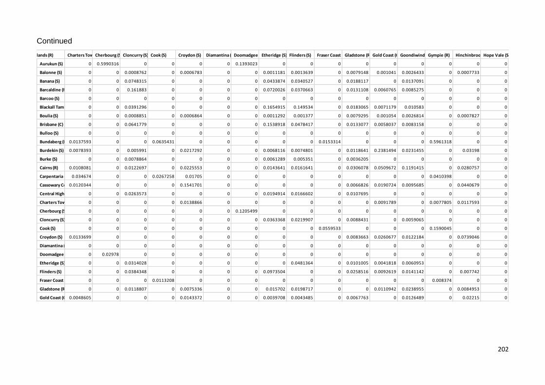
202

Continued

Central Highlands (R) Charters Towers (R) Cherbourg (S) Cloncurry (S) Cook (S) Croydon (S) Diamantina (S) Doomadgee (S) Etheridge (S) Flinders (S) Fraser Coast (R) Gladstone (R) Gold Coast (C) Goondiwindi (R) Gympie (R) Hinchinbrook (S) Hope Vale (S)

Aurukun (S) 0 0.5990316 0 0 0 0 0.1393023 0 0 0 0 0 0 0 0 0

Balonne (S) 0 0 0.0008762 0 0.0006783 0 0 0.0011181 0.0013639 0 0.0079148 0.001041 0.0026433 0 0.0007733 0

Banana (S) 0 0 0.0748315 0 0 0 0 0.0433874 0.0340527 0 0.0188117 0 0.0137091 0 0 0

Barcaldine (R) 0 0 0.161883 0 0 0 0 0.0720026 0.0370663 0 0.0131108 0.0060765 0.0085275 0 0 0

Barcoo (S) 0 0 0 0 0 0 0 0 0 0 0 0 0 0 0 0

Blackall Tambo (R) 0 0 0.0391296 0 0 0 0 0.1654915 0.149534 0 0.0183065 0.0071179 0.010583 0 0 0

Boulia (S) 0 0 0.0008851 0 0.0006864 0 0 0.0011292 0.001377 0 0.0079295 0.001054 0.0026814 0 0.0007827 0

Brisbane (C) 0 0 0.0641779 0 0 0 0 0.1538918 0.0478417 0 0.0133077 0.0058037 0.0083158 0 0 0

Bulloo (S) 0 0 0 0 0 0 0 0 0 0 0 0 0 0 0 0

Bundaberg (R) 0.0137593 0 0 0.0635431 0 0 0 0 0 0.0153314 0 0 0 0.5961318 0 0

Burdekin (S) 0.0078393 0 0.005991 0 0.0217292 0 0 0.0068116 0.0074801 0 0.0118641 0.2381494 0.0231455 0 0.03198 0

Burke (S) 0 0 0.0078864 0 0 0 0 0.0061289 0.005351 0 0.0036205 0 0 0 0 0

Cairns (R) 0.0108081 0 0.0122697 0 0.0225553 0 0 0.0143641 0.0161641 0 0.0306078 0.0509672 0.1191415 0 0.0280757 0

Carpentaria (S) 0.034674 0 0 0.0267258 0.01705 0 0 0 0 0 0 0 0 0.0410398 0 0

Cassowary Coast (R)0.0120344 0 0 0 0.1541701 0 0 0 0 0 0.0066826 0.0190724 0.0095685 0 0.0440679 0

Central Highlands (R) 0 0 0.0263573 0 0 0 0 0.0194914 0.0166602 0 0.0107695 0 0 0 0 0

Charters Towers (R) 0 0 0 0 0.0138866 0 0 0 0 0 0 0.0091789 0 0.0077805 0.0117593 0

Cherbourg (S) 0 0 0 0 0 0 0.1205499 0 0 0 0 0 0 0 0 0

Cloncurry (S) 0 0 0 0 0 0 0 0.0363368 0.0219907 0 0.0088431 0 0.0059065 0 0 0

Cook (S) 0 0 0 0 0 0 0 0 0 0.0559533 0 0 0 0.1590045 0 0

Croydon (S) 0.0133699 0 0 0 0 0 0 0 0 0 0.0083663 0.0260677 0.0122184 0 0.0739046 0

Diamantina (S) 0 0 0 0 0 0 0 0 0 0 0 0 0 0 0 0

Doomadgee (S) 0 0.02978 0 0 0 0 0 0 0 0 0 0 0 0 0 0

Etheridge (S) 0 0 0.0314028 0 0 0 0 0 0.0481364 0 0.0101005 0.0041818 0.0060953 0 0 0

Flinders (S) 0 0 0.0384348 0 0 0 0 0.0973504 0 0 0.0258516 0.0092619 0.0141142 0 0.007742 0

Fraser Coast (R) 0 0 0 0.0113208 0 0 0 0 0 0 0 0 0 0.008374 0 0

Gladstone (R) 0 0 0.0118807 0 0.0075336 0 0 0.015702 0.0198717 0 0 0.0110942 0.0238955 0 0.0084953 0

Gold Coast (C) 0.0048605 0 0 0 0.0143372 0 0 0.0039708 0.0043485 0 0.0067763 0 0.0126489 0 0.02215 0

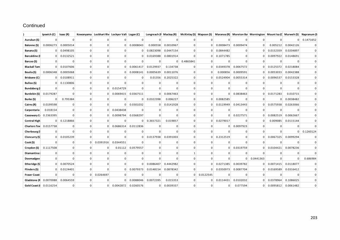
203

Continued


Aurukun (S) 0 0 0 0 0 0 0 0 0 0 0 0 0 0 0 0.1471652

Balonne (S) 0.0006273 0.0005014 0 0 0 0.0008043 0.000558 0.0010967 0 0 0.0008473 0.0009474 0 0.005212 0.0042126 0

Banana (S) 0 0.0498105 0 0 0 0 0.0823098 0.0447154 0 0 0.0844482 0 0 0.0152359 0.0204897 0

Barcaldine (R) 0 0.0132521 0 0 0 0 0.0169388 0.0801914 0 0 0.1071785 0 0 0.0097922 0.0148691 0

Barcoo (S) 0 0 0 0 0 0 0 0 0.4865841 0 0 0 0 0 0 0

Blackall Tambo (R) 0 0.0107606 0 0 0 0.0061417 0.0129937 0.134738 0 0 0.0349378 0.0067572 0 0.0125372 0.0218084 0

Boulia (S) 0.0006348 0.0005068 0 0 0 0.0008141 0.0005639 0.0011076 0 0 0.000856 0.0009591 0 0.0053033 0.0042388 0

Brisbane (C) 0 0.0108911 0 0 0 0 0.01356 0.2025322 0 0 0.0524904 0.0055314 0 0.0096537 0.0153328 0

Bulloo (S) 0 0.1130806 0 0 0 0 0 0 0 0 0 0 0 0 0 0

Bundaberg (R) 0 0 0 0 0.0154729 0 0 0 0 0 0 0 0 0 0 0

Burdekin (S) 0.0179287 0 0 0 0.0069415 0.0367511 0 0.0067463 0 0 0 0.0838463 0 0.0171283 0.010715 0

Burke (S) 0 0.795384 0 0 0 0 0.0322398 0.006227 0 0 0.0082585 0 0 0 0.0038482 0

Cairns (R) 0.0199598 0 0 0 0 0.0301032 0 0.0141928 0 0 0.0119949 0.0413443 0 0.0575938 0.0263066 0

Carpentaria (S) 0.018154 0 0 0 0.0438438 0 0 0 0 0 0 0 0 0 0 0

Cassowary Coast (R)0.2363395 0 0 0 0.0098794 0.0368297 0 0 0 0 0 0.0227571 0 0.0082519 0.0062667 0

Central Highlands (R) 0 0.1218866 0 0 0 0 0.3657321 0.019857 0 0 0.0279017 0 0 0.009085 0.0115144 0

Charters Towers (R)0.0157738 0 0 0 0.0686314 0.0112836 0 0 0 0 0 0.0097923 0 0 0 0

Cherbourg (S) 0 0 0 0 0 0 0 0 0 0 0 0 0 0 0 0.1260124

Cloncurry (S) 0 0.0105239 0 0 0 0 0.0137938 0.0391003 0 0 0.2312519 0 0 0.0067325 0.0099294 0

Cook (S) 0 0 0 0.0391916 0.0344551 0 0 0 0 0 0 0 0 0 0 0

Croydon (S) 0.1117508 0 0 0 0.01112 0.0579557 0 0 0 0 0 0.0319759 0 0.0104421 0.0078236 0

Diamantina (S) 0 0 0 0 0 0 0 0 1 0 0 0 0 0 0 0

Doomadgee (S) 0 0 0 0 0 0 0 0 0 0 0 0 0.0441363 0 0 0.686984

Etheridge (S) 0 0.0070524 0 0 0 0 0.0086407 0.4442982 0 0 0.0271385 0.0039782 0 0.0071415 0.0118077 0

Flinders (S) 0 0.0124401 0 0 0 0.0079373 0.0148154 0.0878342 0 0 0.0350973 0.0087704 0 0.0169589 0.0316412 0

Fraser Coast (R) 0 0 0 0.0264697 0 0 0 0 0 0.0122545 0 0 0 0 0 0

Gladstone (R) 0.0070088 0.0064559 0 0 0 0.0088046 0.0072395 0.015353 0 0 0.0114431 0.0102032 0 0.0378964 0.1086025 0

Gold Coast (C) 0.0116254 0 0 0 0.0042872 0.0260576 0 0.0039337 0 0 0 0.077594 0 0.0095812 0.0061482 0

204

Continued


Aurukun (S) 0 0 0 0 0 0 0 0 0 0 0 0 0 0 0 0 0

Balonne (S) 0.0005462 0 0 0.0006067 0 0 0.1021631 0 0.0008272 0.0005867 0 0 0 0.0004965 0 0.0008004 0

Banana (S) 0 0 0 0 0 0.0179607 0.0173225 0.0210641 0 0 0 0 0 0 0 0 0

Barcaldine (R) 0 0 0 0 0 0.0067015 0.011663 0.0075629 0 0 0 0 0 0 0 0 0

Barcoo (S) 0 0 0 0 0 0 0 0 0 0 0 0 0 0 0 0 0

Blackall Tambo (R) 0 0 0 0 0 0.006073 0.0156659 0.0067506 0.006246 0 0 0 0 0 0 0.0061236 0

Boulia (S) 0.0005527 0 0 0.000614 0 0 0.0921659 0 0.0008373 0.0005937 0 0 0 0.0005024 0 0.0008102 0

Brisbane (C) 0 0 0 0 0 0.0057809 0.0116873 0.0064817 0 0 0 0 0 0 0 0 0

Bulloo (S) 0 0 0 0 0 0.2036459 0 0.1719203 0 0 0 0 0 0 0 0 0

Bundaberg (R) 0 0 0 0 0.0186374 0 0 0 0 0 0.0246555 0.1151896 0.0135938 0 0.0238654 0 0.0359001

Burdekin (S) 0.0133255 0 0 0.0166203 0 0 0.0133692 0 0.04097 0.0154418 0 0 0.0079523 0.0111175 0 0.0360918 0

Burke (S) 0 0 0 0 0 0.0075528 0.0034087 0.009842 0 0 0 0 0 0 0 0 0

Cairns (R) 0.0162636 0 0 0.018977 0 0 0.0369493 0 0.0316825 0.0180476 0 0 0.0109347 0.0142258 0 0.0298394 0

Carpentaria (S)0.0208158 0 0 0.0186989 0 0 0 0 0 0.0193049 0.209629 0.0523065 0.0338951 0.023479 0.1731124 0 0.2105431

Cassowary Coast (R)0.0393729 0 0 0.1104387 0 0 0.0071829 0 0.0330794 0.0709237 0.006434 0 0.0123299 0.0239392 0.0065617 0.0375856 0.0054339

Central Highlands (R) 0 0 0 0 0 0.0174424 0.0100846 0.0217335 0 0 0 0 0 0 0 0 0

Charters Towers (R)0.0215607 0 0 0.0168015 0 0 0 0 0.0109771 0.01803 0.0171989 0.008632 0.6246874 0.0301044 0.0179493 0.0113398 0.0123244

Cherbourg (S) 0 0 0 0 0 0 0 0 0 0 0 0 0 0 0 0 0

Cloncurry (S) 0 0 0 0 0 0.0050972 0.0079323 0.0057845 0 0 0 0 0 0 0 0 0

Cook (S) 0 0 0 0 0.0730268 0 0 0 0 0 0.0491869 0.1133983 0 0 0.048041 0 0.063521

Croydon (S) 0.0375635 0 0 0.077066 0 0 0.0090233 0 0.0504421 0.05818 0.0073973 0 0.0136739 0.0248181 0.007538 0.0595288 0

Diamantina (S) 0 0 0 0 0 0 0 0 0 0 0 0 0 0 0 0 0

Doomadgee (S) 0 0 0.0329374 0 0 0 0 0 0 0 0 0 0 0 0 0 0

Etheridge (S) 0 0 0 0 0 0.0038632 0.0087696 0.0043125 0 0 0 0 0 0 0 0 0

Flinders (S) 0 0 0 0 0 0 0.0216863 0.0080045 0.008078 0 0 0 0 0 0 0.0079129 0

Fraser Coast (R) 0 0.0157152 0 0 0.0484212 0 0 0 0 0 0 0.0075804 0 0 0 0 0

Gladstone (R) 0.0061613 0 0 0.0067958 0 0 0.1034603 0 0.0090315 0.0065864 0 0 0 0 0 0.0087655 0

Gold Coast (C) 0.0084637 0 0 0.0107134 0 0 0.0075902 0 0.0296704 0.0099011 0 0 0.004933 0.0069926 0 0.0255066 0

205

Continued


Aurukun (S) 0 0 0 0 0 0 0.1145009 0 0

Balonne (S) 0 0.0022876 0 0.0010245 0.0052945 0.0008535 0 0 0

Banana (S) 0 0.024406 0.019827 0 0.0197212 0.0821156 0 0 0

Barcaldine (R) 0 0.0195972 0.0072274 0.0060304 0.0140461 0.1158306 0 0 0

Barcoo (S) 0 0 0 0 0 0 0 0 0

Blackall Tambo (R) 0 0.0332507 0.0064892 0.0070565 0.0201264 0.0357852 0 0 0

Boulia (S) 0 0.0023071 0 0.0010373 0.0053207 0.0008623 0 0 0

Brisbane (C) 0 0.0211126 0.0062099 0.0057575 0.014377 0.054692 0 0 0

Bulloo (S) 0 0 0.1821686 0 0 0 0 0 0

Bundaberg (R) 0.015494 0 0 0 0 0 0 0.0191801 0

Burdekin (S) 0 0.0091251 0 0.1831811 0.0111885 0.005904 0 0 0

Burke (S) 0 0.0043392 0.0088711 0 0.0037453 0.0081732 0 0 0

Cairns (R) 0 0.0209983 0 0.0491036 0.0280272 0.0120545 0 0 0

Carpentaria (S) 0 0 0 0 0 0 0 0 0

Cassowary Coast (R) 0 0.0056358 0 0.0195896 0.0064418 0 0 0 0

Central Highlands (R) 0 0.0131509 0.0199602 0 0.0111767 0.0275449 0 0 0

Charters Towers (R) 0 0 0 0.0092736 0 0 0 0 0

Cherbourg (S) 0 0 0 0 0 0 0 0 0.1144955

Cloncurry (S) 0 0.0127458 0.0055159 0 0.0094237 0.296874 0 0 0

Cook (S) 0.0567381 0 0 0 0 0 0 0.0760725 0

Croydon (S) 0 0.007006 0 0.0268774 0.0080518 0 0 0 0

Diamantina (S) 0 0 0 0 0 0 0 0 0

Doomadgee (S) 0 0 0 0 0 0 0.1694572 0 0

Etheridge (S) 0 0.0169664 0.0041387 0.0041472 0.0109958 0.0279783 0 0 0

Flinders (S) 0 0.0529897 0.0077074 0.009178 0.0288214 0.0357842 0 0 0

Fraser Coast (R)0.8184702 0 0 0 0 0 0 0.0428048 0

Gladstone (R) 0 0.0388015 0 0.0109384 0.192855 0.011537 0 0 0

Gold Coast (C) 0 0.0052696 0 0.4758687 0.0064077 0 0 0 0

206

Continued


Goondiwindi (R) 0 0.0528214 0.0107406 0.0138422 0 0.016706 0.0529872 0.0148534 0 0 0.0376518 0 0.1145357 0 0.0171002 0

Gympie (R) 0 0 0 0 0 0 0 0 0 0.5807698 0 0 0 0.0299619 0 0

Hinchinbrook (S) 0 0.0076389 0 0 0 0 0.0076459 0 0 0 0.0257172 0 0.0133423 0 0.0389319 0

Hope Vale (S) 0 0 0 0 0 0 0 0 0 0 0 0 0 0 0 0

Ipswich (C) 0 0.0066818 0 0 0 0 0.0066868 0 0 0 0.0155469 0 0.0102285 0.0057553 0.2251505 0

Isaac (R) 0 0.0033919 0.0132101 0.0072817 0 0.00575 0.0033899 0.0065851 0.0033129 0 0 0.7919532 0 0 0 0.044607

Kowanyama (S) 0 0 0 0 0 0 0 0 0 0 0 0 0 0 0 0

Lockhart River (S) 0 0 0 0 0 0 0 0 0 0 0 0 0 0 0 0

Lockyer Valley (R) 0 0 0 0 0 0 0 0 0 0.0204309 0.0187878 0 0 0.0433838 0.0293761 0

Logan (C) 0 0.0030988 0 0 0 0.0018692 0.0031017 0 0 0 0.0115263 0 0.0055794 0 0.0126899 0

Longreach (R) 0 0.0107067 0.0619189 0.0264008 0 0.0196947 0.0106996 0.023256 0 0 0 0.0910544 0 0 0 0.3796606

Mackay (R) 0 0.0083398 0.0133313 0.0495343 0 0.0809374 0.008329 0.1376614 0 0 0.0041762 0.0069699 0.0051921 0 0 0.0081694

McKinlay (S) 0 0 0 0 0.4814432 0 0 0 0 0 0 0 0 0 0 0

Mapoon (S) 0 0 0 0 0 0 0 0 0 0 0 0 0 0 0 0

Maranoa (R) 0 0.0045175 0.0176519 0.0464163 0 0.0147143 0.0045129 0.025014 0 0 0 0.0064809 0.0030765 0 0 0.0080481

Moreton Bay (R) 0 0.012115 0 0 0 0.0068261 0.0121286 0.0063226 0 0 0.0872859 0 0.0254351 0 0.0260265 0

Mornington (S) 0 0 0 0 0 0 0 0 0 0 0 0 0 0 0 0

Mount Isa (C) 0 0.0926521 0.0106189 0.0141402 0 0.0176058 0.0932273 0.0153393 0 0 0.0247871 0 0.0492544 0 0.0131191 0.0087377

Murweh (S) 0 0.0542675 0.0103487 0.0155596 0 0.0221931 0.0539982 0.0176553 0 0 0.0112369 0.007297 0.0163032 0 0.0072199 0.0080251

Napranum (S) 0.0401534 0 0 0 0 0 0 0 0 0 0 0 0 0 0 0

North Burnett (R) 0 0.0102859 0 0 0 0 0.0102926 0 0 0 0.0204291 0 0.0147346 0.0116669 0.0663135 0

Northern Peninsula Area (R)0 0 0 0 0 0 0 0 0 0 0 0 0 0 0 0

Palm Island (S) 0 0 0 0 0 0 0 0 0 0 0 0 0 0 0 0

Paroo (S) 0 0.0068789 0 0 0 0 0.0068838 0 0 0 0.0153395 0 0.0103503 0.0063093 0.1119775 0

Pormpuraaw (S) 0 0 0 0 0 0 0 0 0 0.0186829 0 0 0 0 0 0

Quilpie (S) 0 0 0.03176 0.0245523 0 0.0216375 0 0.0233055 0.0397804 0 0 0.0501418 0 0 0 0.0425621

Redland (C) 0 0.4133275 0.0027477 0.003833 0 0.0050068 0.368737 0.0042265 0 0 0.0044032 0.00203 0.0071916 0 0.002599 0.0022074

Richmond (S) 0 0 0.0274658 0.0204315 0 0.0177352 0 0.0192682 0.0247635 0 0 0.0481805 0 0 0 0.0391056

Rockhampton (R) 0 0.007292 0 0 0 0.0043494 0.0072991 0 0 0 0.0294003 0 0.0134357 0 0.0260785 0

207

Continued


Goondiwindi (R) 0 0 0.0131495 0 0.0182318 0 0 0.0157019 0.0179784 0 0.0395971 0.0343166 0 0 0.021843 0

Gympie (R) 0.0137214 0 0 0.0559426 0 0 0 0 0 0.0145618 0 0 0 0 0 0

Hinchinbrook (S)0.0083512 0 0 0 0.0545142 0 0 0 0.0048749 0 0.006959 0.0297063 0.0107978 0 0 0

Hope Vale (S) 0 0 0 0 0 0 0 0 0 0 0 0 0 0 0 0

Ipswich (C) 0.0120798 0 0 0 0.0888876 0 0 0 0 0 0.0061911 0.0168127 0.0087608 0 0.0353839 0

Isaac (R) 0 0 0.007931 0 0 0 0 0.0061499 0.005364 0 0.0036213 0 0 0 0 0

Kowanyama (S) 0 0 0 0 0 0 0 0 0 0 0 0 0 0 0 0.5006389

Lockhart River (S) 0 0 0 0.0489856 0 0 0 0 0 0.1635214 0 0 0 0 0 0.0424117

Lockyer Valley (R)0.164048 0 0 0.0164301 0.027607 0 0 0 0 0 0 0.0193519 0 0.0209753 0.0239964 0

Logan (C) 0.0031253 0 0 0 0.0166729 0 0 0 0.0019492 0 0.0028129 0.0136296 0.004454 0 0.0772596 0

Longreach (R) 0 0 0.0294861 0 0 0 0 0.0213728 0.0181201 0 0.0115188 0 0 0 0 0

Mackay (R) 0 0 0.0331252 0 0 0 0 0.435542 0.042575 0 0.0096814 0.0040612 0.0058943 0 0 0

McKinlay (S) 0 0 0 0 0 0.5185568 0 0 0 0 0 0 0 0 0 0

Mapoon (S) 0 0 0 0 0 0 0 0 0 0.0874029 0 0 0 0 0 0.0700372

Maranoa (R) 0 0 0.1373563 0 0 0 0 0.0186521 0.0119275 0 0.0050591 0 0.0034209 0 0 0

Moreton Bay (R)0.0090026 0 0 0 0.0305336 0 0 0.0065583 0.0071491 0 0.0108199 0.1347159 0.0188825 0 0.0538193 0

Mornington (S) 0 0 0 0 0 0 0.1232541 0 0 0 0 0 0 0 0 0.1040793

Mount Isa (C) 0 0 0.0133336 0 0.013861 0 0 0.0163659 0.0192169 0 0.0558646 0.0231239 0.0953447 0 0.0161417 0

Murweh (S) 0 0 0.0142506 0 0.0075258 0 0 0.019609 0.0259824 0 0.116016 0.010753 0.020923 0 0.0084168 0

Napranum (S) 0 0.0322344 0 0 0 0 0.7113692 0 0 0 0 0 0 0 0 0

North Burnett (R)0.0291913 0 0 0 0.0528232 0 0 0 0 0 0.009622 0.02164 0.0129649 0 0.0350223 0

Northern Peninsula Area (R)0 0 0 0 0 0 0 0 0 0.0956031 0 0 0 0 0 0.0507774

Palm Island (S) 0 0 0 0 0 0 0.0920221 0 0 0 0 0 0 0 0 0.1460635

Paroo (S) 0.0136944 0 0 0 0.0652419 0 0 0 0 0 0.0063891 0.0164903 0.0089282 0 0.0319379 0

Pormpuraaw (S) 0 0 0 0.0264369 0 0 0 0 0 0.0866393 0 0 0 0.0181165 0 0

Quilpie (S) 0 0 0.0256126 0 0 0 0 0.0224617 0 0 0 0 0 0 0 0

Redland (C) 0 0 0.0035754 0 0.002726 0 0 0.0045738 0.0055927 0 0.0347106 0.0041691 0.0104246 0 0.0031051 0

Richmond (S) 0 0 0.0214328 0 0 0 0 0.0184894 0.0169691 0 0 0 0 0 0 0

Rockhampton (R)0.0069566 0 0 0 0.0332026 0 0 0 0.004539 0 0.006602 0.0355091 0.0106134 0 0.1045852 0

208

Continued


Goondiwindi (R)0.0164349 0 0 0 0 0.0231023 0 0.0154894 0 0 0.012822 0.0295066 0 0.1071779 0.0324559 0

Gympie (R) 0 0 0 0 0.0154758 0 0 0 0 0 0 0 0 0 0 0

Hinchinbrook (S)0.0328135 0 0 0 0.0071296 0.1980964 0 0 0 0 0 0.041574 0 0.0089698 0.0064541 0

Hope Vale (S) 0 0 0.5219549 0.067516 0 0 0 0 0 0.0965706 0 0 0.0965033 0 0 0

Ipswich (C) 0 0 0 0 0.0098223 0.0303556 0 0 0 0 0 0.0197755 0 0.007596 0.0058158 0

Isaac (R) 0 0 0 0 0 0 0.0334569 0.006249 0 0 0.0083091 0 0 0 0.0038502 0

Kowanyama (S) 0 0 0 0 0 0 0 0 0 0.0781649 0 0 0.1135577 0 0 0

Lockhart River (S) 0 0 0 0 0 0 0 0 0 0.1409664 0 0 0 0 0 0

Lockyer Valley (R)0.0306576 0 0 0 0 0.0231628 0 0 0 0 0 0.0204836 0 0 0 0

Logan (C) 0.010979 0 0 0 0.002684 0 0 0 0 0 0 0.020521 0 0.0036642 0.002602 0

Longreach (R) 0 0.094901 0 0 0 0 0 0.0217967 0 0 0.0313565 0 0 0.0096713 0.0123415 0

Mackay (R) 0 0.0070249 0 0 0 0 0.0086384 0 0 0 0.0283344 0.0038652 0 0.00689 0.0112753 0

McKinlay (S) 0 0 0 0 0 0 0 0 0 0 0 0 0 0 0 0

Mapoon (S) 0 0 0.0591023 0.1627501 0 0 0 0 0 0 0 0 0 0 0 0

Maranoa (R) 0 0.0065489 0 0 0 0 0.0087127 0.0198655 0 0 0 0 0 0.0038858 0.0056549 0

Moreton Bay (R)0.0237405 0 0 0 0.0078785 0.0681143 0 0.0065001 0 0 0 0 0 0.0148063 0.0098906 0

Mornington (S) 0 0 0.1276872 0 0 0 0 0 0 0 0 0 0 0 0 0.1158135

Mount Isa (C) 0.0126765 0 0 0 0 0.0169073 0.0089603 0.016107 0 0 0.0129564 0.0205825 0 0 0.0414135 0

Murweh (S) 0.0070334 0.0073324 0 0 0 0.0087002 0.008286 0.0191014 0 0 0.0136639 0.0099636 0 0.0300111 0 0

Napranum (S) 0 0 0 0 0 0 0 0 0 0 0 0 0.042944 0 0 0

North Burnett (R)0.0795693 0 0 0 0.022213 0.0320501 0 0 0 0 0 0.0242894 0 0.01149 0.0091054 0

Northern Peninsula Area (R)0 0 0.043877 0.2353059 0 0 0 0 0 0.3385274 0 0 0 0 0 0

Palm Island (S) 0 0 0.1972101 0 0 0 0 0 0 0 0 0 0.3626687 0 0 0.0878119

Paroo (S) 0.2102028 0 0 0 0.0110012 0.028004 0 0 0 0 0 0.0191318 0 0.0077852 0.0060128 0

Pormpuraaw (S) 0 0 0 0.0306221 0 0 0 0 0 0.0174982 0 0 0 0 0 0

Quilpie (S) 0 0.0496701 0 0 0 0 0.0406247 0.0226587 0 0 0.0261899 0 0 0 0 0

Redland (C) 0.0025223 0.0020387 0 0 0 0.0032287 0.00227 0.0044853 0 0 0.0034568 0.0037976 0 0.020063 0.0177762 0

Richmond (S) 0 0.0475916 0 0 0 0 0.0369121 0.0186706 0 0 0.0219826 0 0 0 0 0

Rockhampton (R)0.0228766 0 0 0 0.0059974 0.2561061 0 0 0 0 0 0.0574935 0 0.0086677 0.0060951 0

209

Continued


Goondiwindi (R)0.013757 0 0 0.0157368 0 0 0.0514892 0 0.0240597 0.0150675 0 0 0.0096283 0.0122171 0 0.0229403 0

Gympie (R) 0 0 0 0 0.0176067 0 0 0 0 0 0.0250565 0.1390991 0.0135526 0 0.02422 0 0.0372162

Hinchinbrook (S)0.0183707 0 0 0.0278279 0 0 0.0075815 0 0.1172004 0.0240121 0.00496 0 0.0085115 0.0137044 0.0050456 0.2257375 0

Hope Vale (S) 0 0.0820855 0.1353696 0 0 0 0 0 0 0 0 0 0 0 0 0 0

Ipswich (C) 0.0450068 0 0 0.1974992 0 0 0.006641 0 0.0276441 0.0965355 0.0063009 0 0.0123927 0.0253762 0.0064295 0.0308932 0.0052984

Isaac (R) 0 0 0 0 0 0.0074495 0.0034086 0.0096798 0 0 0 0 0 0 0 0 0

Kowanyama (S) 0 0.0680339 0.1753075 0 0 0 0 0 0 0 0 0 0 0 0 0 0

Lockhart River (S) 0 0.2389502 0 0 0.1057259 0 0 0 0 0 0 0 0 0 0 0 0

Lockyer Valley (R)0.0392162 0 0 0.0322621 0 0 0 0 0.0226203 0.0341303 0.0548572 0.0236011 0.1478089 0.0500179 0.0580983 0.0232617 0.0359066

Logan (C) 0.0065567 0 0 0.0095163 0 0 0.0030745 0 0.1119321 0.0083525 0.0018872 0 0.0031828 0.004999 0.001919 0.6309587 0

Longreach (R) 0 0 0 0 0 0.0172824 0.0107655 0.0212957 0 0 0 0 0 0 0 0 0

Mackay (R) 0 0 0 0 0 0.0038203 0.0084303 0.004269 0 0 0 0 0 0 0 0 0

McKinlay (S) 0 0 0 0 0 0 0 0 0 0 0 0 0 0 0 0 0

Mapoon (S) 0 0.3968937 0 0 0.0697504 0 0 0 0 0 0 0 0 0 0 0 0

Maranoa (R) 0 0 0 0 0 0.0030958 0.0045553 0.003524 0 0 0 0 0 0 0 0 0

Moreton Bay (R)0.0164935 0 0 0.0215798 0 0 0.0120036 0 0.0834053 0.0197041 0 0 0.009146 0.0133427 0 0.0659687 0

Mornington (S) 0 0 0.3625034 0 0 0 0 0 0 0 0 0 0 0 0 0 0

Mount Isa (C) 0.010846 0 0 0.012207 0 0 0.0881548 0 0.0174795 0.0117518 0 0 0 0.0097561 0 0.0168096 0

Murweh (S) 0.0062285 0 0 0.0068322 0 0 0.0566014 0 0.0089073 0.0066337 0 0 0 0 0 0.0086645 0

Napranum (S) 0 0 0.0325461 0 0 0 0 0 0 0 0 0 0 0 0 0 0

North Burnett (R) 0 0 0 0.1030534 0 0 0.0102312 0 0.0302766 0.1490675 0.0129531 0 0.0302348 0.1028585 0.0132615 0.0323867 0.0106172

Northern Peninsula Area (R)0 0 0 0 0.0721777 0 0 0 0 0 0 0 0 0 0 0 0

Palm Island (S) 0 0 0 0 0 0 0 0 0 0 0 0 0 0 0 0 0

Paroo (S) 0.0620395 0 0 0 0 0 0.0068383 0 0.0258097 0.2009836 0.0069272 0 0.0140729 0.0309904 0.0070734 0.0284328 0.0057947

Pormpuraaw (S) 0 0.0212291 0 0 0 0 0 0 0 0 0 0.016081 0 0 0 0 0.0122983

Quilpie (S) 0 0 0 0 0 0 0 0.2155692 0 0 0 0 0 0 0 0 0

Redland (C) 0.002198 0 0 0.0024403 0 0 0 0 0.0033199 0.00236 0 0 0 0.0019991 0 0.003213 0

Richmond (S) 0 0 0 0 0 0.1589567 0 0 0 0 0 0 0 0 0 0 0

Rockhampton (R)0.0141719 0 0 0.0200677 0 0 0.0072334 0 0 0.0177839 0.0042464 0 0.0070811 0.010949 0.0043167 0.2175183 0

210

Continued


Goondiwindi (R) 0 0.0245056 0 0.0334281 0.0352317 0.012893 0 0 0

Gympie (R) 0.0147123 0 0 0 0 0 0 0.0181034 0

Hinchinbrook (S) 0 0.0057091 0 0.0311565 0.0066654 0 0 0 0

Hope Vale (S) 0 0 0 0 0 0 0 0 0

Ipswich (C) 0 0.0052439 0 0.0172337 0.005974 0 0 0 0

Isaac (R) 0 0.0043441 0.0087354 0 0.0037468 0.0082225 0 0 0

Kowanyama (S) 0 0 0 0 0 0 0.064297 0 0

Lockhart River (S)0.1583987 0 0 0 0 0 0 0.1010401 0

Lockyer Valley (R) 0 0 0 0.0195278 0 0 0 0 0

Logan (C) 0 0.0022927 0 0.0144192 0.0026901 0 0 0 0

Longreach (R) 0 0.0141609 0.0196481 0 0.0119681 0.0309229 0 0 0

Mackay (R) 0 0.0160203 0.0040953 0.0040279 0.0105187 0.0292701 0 0 0

McKinlay (S) 0 0 0 0 0 0 0 0 0

Mapoon (S) 0.0861136 0 0 0 0 0 0 0.0679498 0

Maranoa (R) 0 0.0071751 0.0033563 0 0.0053782 0.6213993 0 0 0

Moreton Bay (R) 0 0.0085671 0 0.160962 0.0102762 0 0 0 0

Mornington (S) 0 0 0 0 0 0 0.1666626 0 0

Mount Isa (C) 0 0.0282619 0 0.0226676 0.0466899 0.013038 0 0 0

Murweh (S) 0 0.0644918 0 0.0106159 0.2655622 0.0137894 0 0 0

Napranum (S) 0 0 0 0 0 0 0.1407529 0 0

North Burnett (R) 0 0 0 0.0220318 0.0093241 0 0 0 0

Northern Peninsula Area (R)0.0938021 0 0 0 0 0 0 0.0699294 0

Palm Island (S) 0 0 0 0 0 0 0.1142237 0 0

Paroo (S) 0 0.0054369 0 0.0168701 0.0061716 0 0 0 0

Pormpuraaw (S)0.0920873 0 0 0 0 0 0 0.6603085 0

Quilpie (S) 0 0 0.3374135 0 0 0.02606 0 0 0

Redland (C) 0 0.0094672 0 0.0041037 0.0225912 0.0034823 0 0 0

Richmond (S) 0 0 0.4401861 0 0 0.0218587 0 0 0

Rockhampton (R) 0 0.0053554 0 0.0378703 0.0063066 0 0 0 0

211

Continued


Scenic Rim (R) 0 0.007862 0 0 0 0 0.0078675 0 0 0 0.0168461 0 0.0116353 0.0076996 0.0850027 0

Somerset (R) 0 0 0 0 0 0 0 0 0 0.0183417 0 0 0 0.1168637 0.0107784 0

South Burnett (R) 0 0 0 0 0 0 0 0 0 0.2012143 0 0 0 0.0684706 0 0

Southern Downs (R) 0 0 0 0 0 0 0 0 0 0.00748 0.0089692 0 0.0072883 0.0139764 0.0152778 0

Sunshine Coast (R) 0 0.0125452 0 0 0 0 0.0125526 0 0 0 0.0228664 0 0.0172912 0.017655 0.0540929 0

Tablelands (R) 0 0 0 0 0 0 0 0 0 0.0181565 0 0 0 0.0986947 0.0112414 0

Toowoomba (R) 0 0.0031035 0 0 0 0.0018757 0.0031065 0 0 0 0.0113927 0 0.0055663 0 0.013034 0

Torres (S) 0 0 0 0 0 0 0 0 0 0.0566302 0 0 0 0.2488838 0.0193022 0

Torres Strait Island (R) 0 0 0 0 0 0 0 0 0 0.0086415 0 0 0 0 0 0

Townsville (C) 0 0.0441732 0.0184768 0.030739 0 0.0507196 0.0440539 0.0364398 0 0 0.014344 0.0123331 0.0195063 0 0.0097325 0.0137387

Weipa (T) 0 0 0.0242372 0.0183051 0 0.015983 0 0.0173065 0.0246 0 0 0.0407134 0 0 0 0.0336706

Western Downs (R) 0 0.0076373 0 0.0036518 0 0.0041555 0.0076465 0.0038364 0 0 0.1111664 0 0.0176102 0 0.0130604 0

Whitsunday (R) 0 0.060939 0.0088994 0.0131325 0 0.0182994 0.0605594 0.014791 0 0 0.0104833 0.0063452 0.0155191 0 0.006631 0.0069599

Winton (S) 0 0.0043436 0.0163837 0.0478821 0 0.0143858 0.0043392 0.0248779 0 0 0.0024459 0.0061223 0.0029512 0 0 0.0075838

Woorabinda (S)0.0653021 0 0 0 0 0 0 0 0 0 0 0 0 0 0 0

Wujal Wujal (S) 0 0 0 0 0 0 0 0 0 0.0196393 0 0 0 0 0 0

Yarrabah (S) 0 0 0 0 0 0 0 0 0 0 0 0 0 0 0 0

212

Continued


Scenic Rim (R) 0.0173709 0 0 0 0.0582196 0 0 0 0 0 0.0073195 0.0180141 0.0101047 0 0.0325753 0

Somerset (R) 0.023161 0 0 0.0132144 0.0103466 0 0 0 0 0 0 0 0 0.019133 0.0094052 0

South Burnett (R)0.0272952 0 0 0.0715358 0 0 0 0 0 0.0236352 0 0 0 0.2494068 0 0

Southern Downs (R)0.6222284 0 0 0 0.0141465 0 0 0 0 0 0 0.0092791 0.0066756 0.0076545 0.0119377 0

Sunshine Coast (R)0.0546823 0 0 0 0.0468224 0 0 0 0 0 0 0.0239861 0.0154468 0 0.0350516 0

Tablelands (R) 0.0247196 0 0 0.0131992 0.0107825 0 0 0 0 0 0 0 0 0.0189137 0.0097845 0

Toowoomba (R)0.0031612 0 0 0 0.0172361 0 0 0 0.0019558 0 0.0028185 0.0134277 0.0044514 0 0.0886088 0

Torres (S) 0.0351925 0 0 0.0361861 0 0 0 0 0 0 0 0 0 0.0602592 0 0

Torres Strait Island (R) 0 0 0 0.011428 0 0 0 0 0 0.8147969 0 0 0 0.0084226 0 0

Townsville (C) 0 0 0.0274196 0 0.0101018 0 0 0.0422339 0.0652227 0 0.062131 0.0138147 0.0236798 0 0.0111597 0

Weipa (T) 0 0 0.0191605 0 0 0 0 0.0166353 0.0153182 0 0 0 0 0 0 0

Western Downs (R)0.0049701 0 0 0 0.0149615 0 0 0.0039856 0.0043613 0 0.006762 0.4816268 0.0124705 0 0.0235124 0

Whitsunday (R) 0 0 0.012084 0 0.0069201 0 0 0.0163152 0.0211455 0 0.1840716 0.0100129 0.0202928 0 0.0077662 0

Winton (S) 0 0 0.1683147 0 0 0 0 0.0183548 0.0116079 0 0.0048687 0 0.0032834 0 0 0

Woorabinda (S) 0 0 0 0 0 0 0.3667832 0 0 0 0 0 0 0 0 0

Wujal Wujal (S) 0 0 0 0.0281302 0 0 0 0 0 0.0782326 0 0 0 0.0190271 0 0

Yarrabah (S) 0 1 0 0 0 0 0 0 0 0 0 0 0 0 0 0

213

Continued


Scenic Rim (R) 0.1214484 0 0 0 0.0137569 0.0290536 0 0 0 0 0 0.020649 0 0.0088592 0.0069009 0

Somerset (R) 0.01108 0 0 0 0.0309059 0.0091754 0 0 0 0 0 0 0 0 0 0

South Burnett (R) 0 0 0 0 0.031222 0 0 0 0 0 0 0 0 0 0 0

Southern Downs (R)0.0161188 0 0 0 0.0615942 0.0114459 0 0 0 0 0 0.009909 0 0 0 0

Sunshine Coast (R)0.0601896 0 0 0 0.0380097 0.0327837 0 0 0 0 0 0.0263618 0 0.0138662 0 0

Tablelands (R) 0.0115625 0 0 0 0.0334741 0.0095415 0 0 0 0 0 0 0 0 0 0

Toowoomba (R)0.0112456 0 0 0 0.0027129 0.6350359 0 0 0 0 0 0.020003 0 0.0036666 0.002608 0

Torres (S) 0.0197564 0 0 0 0.0428953 0 0 0 0 0 0 0 0 0 0 0

Torres Strait Island (R) 0 0 0 0.0255254 0 0 0 0 0 0.0120195 0 0 0 0 0 0

Townsville (C) 0.0095059 0.0124007 0 0 0 0.0114909 0.0142512 0.0406805 0 0 0.0259873 0.0129362 0 0.0306989 0.0966688 0

Weipa (T) 0 0.0402643 0 0 0 0 0.0319281 0.0167917 0 0 0.0196287 0 0 0 0 0

Western Downs (R)0.0120607 0 0 0 0.0043785 0.0279006 0 0.0039487 0 0 0 0.0938331 0 0.0095057 0.0061432 0

Whitsunday (R) 0.006455 0.0063753 0 0 0 0.0080367 0.0071792 0.0159212 0 0 0.0116109 0.0092491 0 0.0302302 0.2372707 0

Winton (S) 0 0.0061859 0 0 0 0 0.0082015 0.0195883 0 0 0.5931404 0 0 0.0037324 0.0054473 0

Woorabinda (S) 0 0 0.0560359 0 0 0 0 0 0 0 0 0 0.1291762 0 0 0.2942108

Wujal Wujal (S) 0 0 0 0.0298926 0 0 0 0 0 0.0174121 0 0 0 0 0 0

Yarrabah (S) 0 0 0 0 0 0 0 0 0 0 0 0 0 0 0 0

214

Continued


Scenic Rim (R) 0.1060767 0 0 0.2375703 0 0 0.0078171 0 0.0270361 0 0.0084806 0 0.0178872 0.0433099 0.008666 0.0294434 0.0070529

Somerset (R) 0.0128837 0 0 0.0114451 0 0 0 0 0.0090233 0.0118537 0 0.0233368 0.0225404 0.0147399 0.5540098 0.009203 0.058559

South Burnett (R) 0 0 0 0 0.0280221 0 0 0 0 0 0.0547975 0 0.0269231 0.0212127 0.0525826 0 0.0911042

Southern Downs (R)0.0222436 0 0 0.0171979 0 0 0 0 0.0111295 0.0184928 0.0166722 0.0084808 0 0.0315041 0.0173793 0.011504 0.0120384

Sunshine Coast (R)0.1379962 0 0 0.0690634 0 0 0.0124845 0 0.0313821 0.0816539 0.0198818 0.0121853 0.0574509 0 0.0204252 0.0330455 0.0158837

Tablelands (R) 0.0134895 0 0 0.0119515 0 0 0 0 0.0093807 0.0123875 0.5665715 0.0229013 0.0240291 0.0154862 0 0.0095706 0.0541618

Toowoomba (R)0.0066684 0 0 0.0097245 0 0 0.0030794 0 0.0956815 0.0085193 0.0019051 0 0.0032196 0.0050715 0.0019373 0 0

Torres (S) 0.0223926 0 0 0.020301 0.0193526 0 0 0 0 0.0209037 0.1241712 0.0822708 0.0345116 0.02497 0.1123009 0 0

Torres Strait Island (R) 0 0.01535 0 0 0.051235 0 0 0 0 0 0 0.0076169 0 0 0 0 0

Townsville (C) 0 0 0 0.00926 0 0 0.045185 0 0.0117312 0 0 0 0 0 0 0.0114493 0

Weipa (T) 0 0 0 0 0 0.2332549 0 0.4126791 0 0 0 0 0 0 0 0 0

Western Downs (R)0.0087213 0 0 0.0110928 0 0 0.0075614 0 0.0320263 0.0102338 0 0 0.005045 0.0071827 0 0.0272773 0

Whitsunday (R)0.0056986 0 0 0.0062655 0 0 0.0642697 0 0.0082346 0.0060789 0 0 0 0 0 0.0080025 0

Winton (S) 0 0 0 0 0 0.0029404 0.0043802 0.0033447 0 0 0 0 0 0 0 0 0

Woorabinda (S) 0 0 0.0884918 0 0 0 0 0 0 0 0 0 0 0 0 0 0

Wujal Wujal (S) 0 0.0210089 0 0 0.6744709 0 0 0 0 0 0 0.0168359 0 0 0 0 0.0128004

Yarrabah (S) 0 0 0 0 0 0 0 0 0 0 0 0 0 0 0 0 0

215

Continued


Scenic Rim (R) 0 0 0 0.0183969 0.0070777 0 0 0 0

Somerset (R) 0 0 0 0 0 0 0 0 0

South Burnett (R)0.0238562 0 0 0 0 0 0 0.0287216 0

Southern Downs (R) 0 0 0 0.0093763 0 0 0 0 0

Sunshine Coast (R) 0 0 0 0.0243438 0 0 0 0 0

Tablelands (R) 0 0 0 0 0 0 0 0 0

Toowoomba (R) 0 0.0022991 0 0.0141881 0.002696 0 0 0 0

Torres (S) 0 0 0 0 0 0 0 0.0197199 0

Torres Strait Island (R) 0 0 0 0 0 0 0 0.0449643 0

Townsville (C) 0 0 0 0.0136634 0.07778 0.0262908 0 0 0

Weipa (T) 0 0 0 0 0 0.0195233 0 0 0

Western Downs (R) 0 0.0052749 0 0 0.0063991 0 0 0 0

Whitsunday (R) 0 0.0463622 0 0.0098799 0 0.0117122 0 0 0

Winton (S) 0 0.0069288 0.0031865 0 0.0051784 0 0 0 0

Woorabinda (S) 0 0 0 0 0 0 0 0 0

Wujal Wujal (S)0.0825499 0 0 0 0 0 0 0 0

Yarrabah (S) 0 0 0 0 0 0 0 0 0

216

Table B5: Mean Square Prediction Error

LogEMP ESTIMATED y

GEO MAT y-geoyhat TOU MAT y-TOUyhat EMP MAT Aurukun (S) 3.11 2.277 0.693889 2.9498 0.025664 2.3281 0.6113676

Balonne (S) 5.37 5.07 0.09 4.7465 0.3887523 4.8314 0.29009

Banana (S) 6.55 5.5804 0.9401242 6.0793 0.2215585 6.0984 0.2039426

Barcaldine (R) 5.02 5.3946 0.1403252 5.3627 0.1174433 5.9146 0.8003092

Barcoo (S) 2.83 3.3822 0.3049248 3.6841 0.7294868 3.7536 0.853037

Blackall Tambo (R) 4.73 4.2815 0.2011523 4.7834 0.0028516 4.5789 0.0228312

Boulia (S) 2.87 2.4007 0.2202425 3.0316 0.0261146 3.6609 0.6255228

Brisbane (C) 11.01 11.4314 0.177578 11.5437 0.2848357 11.5767 0.3211489

Bulloo (S) 3.07 4.167 1.203409 3.5678 0.2478048 3.7976 0.5294018

Bundaberg (R) 8.22 8.2057 0.0002045 6.8714 1.818722 8.5056 0.0815674

Burdekin (S) 6.65 5.5531 1.2031896 6.3811 0.0723072 6.4055 0.0597803

Burke (S) 3.36 4.1821 0.6758484 3.4312 0.0050694 3.2197 0.0196841

Cairns (R) 9.24 8.4084 0.6915586 8.9661 0.0750212 8.2311 1.0178792

Carpentaria (S) 4.59 4.5181 0.0051696 4.8332 0.0591462 5.0511 0.2126132

Cassowary Coast (R) 7.22 7.708 0.238144 7.8064 0.343865 7.8279 0.3695424

Central Highlands (R) 7.36 6.7363 0.3890017 7.4343 0.0055205 7.7412 0.1453134

Charters Towers (R) 6.32 5.8549 0.216318 6.0193 0.0904205 6.5078 0.0352688

Cherbourg (S) 2.57 3.0079 0.1917564 2.6805 0.0122103 2.2911 0.0777852

Cloncurry (S) 5.27 4.666 0.364816 4.8564 0.171065 4.6532 0.3804422

Cook (S) 5.38 5.6803 0.0901801 5.1981 0.0330876 5.5642 0.0339296

Croydon (S) 2.56 2.8534 0.0860836 2.6476 0.0076738 4.4918 3.7318512

Diamantina (S) 3.14 3.0201 0.014376 3.112 0.000784 2.4019 0.5447916

Doomadgee (S) 2.91 3.2615 0.1235523 3.2998 0.151944 3.1969 0.0823116

Etheridge (S) 3.83 2.6783 1.3264129 3.8951 0.004238 3.8705 0.0016402

Flinders (S) 4.64 4.562 0.006084 4.5582 0.0066912 4.3691 0.0733868

Fraser Coast (R) 8.26 7.575 0.469225 7.8211 0.1926332 7.6564 0.364333

Gladstone (R) 8.06 8.2667 0.0427249 8.4373 0.1423553 8.4258 0.1338096

Gold Coast (C) 10.31 10.0192 0.0845646 10.828 0.268324 11.1155 0.6488303

Goondiwindi (R) 6.32 7.0213 0.4918217 6.6956 0.1410754 6.0581 0.0685916

Gympie (R) 7.58 7.5771 8.41E-06 7.7492 0.0286286 7.9938 0.1712304

Hinchinbrook (S) 6.29 6.0514 0.05693 6.1617 0.0164609 5.787 0.253009

Hope Vale (S) 3.07 3.1498 0.006368 2.7722 0.0886848 2.8631 0.0428076

Ipswich (C) 9.01 8.6293 0.1449325 7.888 1.258884 6.831 4.748041

Isaac (R) 7.08 7.5279 0.2006144 7.148 0.004624 6.5219 0.3114756

Kowanyama (S) 3.01 3.3174 0.0944948 3.138 0.016384 2.844 0.027556

Lockhart River (S) 2.77 3.0388 0.0722534 3.6805 0.8290103 3.1691 0.1592808

Lockyer Valley (R) 7.42 7.5846 0.0270932 7.4087 0.0001277 7.2848 0.018279

Logan (C) 9.56 9.544 0.000256 8.5248 1.071639 8.9845 0.3312003

Longreach (R) 5.52 5.523 9E-06 5.7082 0.0354192 5.7746 0.0648212

Mackay (R) 8.75 9.2398 0.239904 8.4767 0.0746929 8.2557 0.2443325

McKinlay (S) 4.05 4.562 0.262144 4.0313 0.0003497 4.3112 0.0682254

Mapoon (S) 1.73 3.0577 1.7627873 3.48 3.0625 3.5193 3.2015945

Maranoa (R) 6.53 6.7391 0.0437228 6.2859 0.0595848 6.5959 0.0043428

Moreton Bay (R) 9.89 9.7596 0.0170042 10.0297 0.0195161 9.761 0.016641

Mornington (S) 3.29 2.8537 0.1903577 3.0584 0.0536386 2.6745 0.3788403

Mount Isa (C) 6.91 6.3496 0.3140482 5.8273 1.1722393 6.2864 0.388877

Murweh (S) 5.45 4.701 0.561001 5.0513 0.1589617 5.2011 0.0619512

Napranum (S) 2.48 2.1806 0.0896404 2.3986 0.006626 1.8082 0.4513152

North Burnett (R) 6.07 6.322 0.063504 6.2554 0.0343732 6.2673 0.0389273

Northern Peninsula Area (R) 4.17 3.8237 0.1199237 3.416 0.568516 3.3071 0.7445964

Palm Island (S) 3.79 4.8925 1.2155063 5.4467 2.7446549 5.634 3.400336

Paroo (S) 4.33 3.8049 0.27573 3.51 0.6724 5.3937 1.1314577

Pormpuraaw (S) 3.06 3.1846 0.0155252 2.8958 0.0269616 3.4546 0.1557092

Quilpie (S) 4.08 4.7695 0.4754103 3.586 0.244036 4.1427 0.0039313

Redland (C) 8.92 8.9963 0.0058217 8.2892 0.3979086 7.9164 1.007213

Richmond (S) 3.74 4.3987 0.4338857 4.0304 0.0843322 3.8457 0.0111725

Rockhampton (R) 8.68 8.7865 0.0113423 9.165 0.235225 8.8439 0.0268632

Scenic Rim (R) 7.52 7.6624 0.0202778 7.0399 0.230496 7.1194 0.1604804

Somerset (R) 6.84 7.2739 0.1882692 6.6317 0.0433889 6.9328 0.0086118

South Burnett (R) 7.12 6.0902 1.060488 6.7787 0.1164857 6.3997 0.5188321

Southern Downs (R) 7.45 7.32 0.0169 7.0262 0.1796064 7.275 0.030625

Sunshine Coast (R) 9.72 10.0244 0.0926594 10.148 0.183184 10.4765 0.5722922

Tablelands (R) 7.58 7.7046 0.0155252 7.3995 0.0325803 7.4324 0.0217858

217

Toowoomba (R) 8.92 8.1759 0.5536848 7.618 1.695204 8.0667 0.7281209

Torres (S) 5.04 4.4434 0.3559316 5.5423 0.2523053 4.9286 0.01241

Torres Strait Island (R) 4.84 3.9794 0.7406324 3.0616 3.1627066 4.2059 0.4020828

Townsville (C) 9.21 9.0523 0.0248693 8.9681 0.0585156 8.2518 0.9181472

Weipa (T) 5.14 5.0729 0.0045024 5.6155 0.2261003 5.4715 0.1098923

Western Downs (R) 7.32 8.1736 0.728633 8.3363 1.0328657 8.4586 1.29641

Whitsunday (R) 7.75 7.6965 0.0028622 7.1605 0.3475103 7.4363 0.0984077

Winton (S) 4.32 4.3311 0.0001232 5.6062 1.6543104 4.4691 0.0222308

Woorabinda (S) 2.67 3.7484 1.1629466 2.8754 0.0421892 2.8547 0.0341141

Wujal Wujal (S) 1.86 3.1716 1.7202946 3.4353 2.4815701 2.6176 0.5739578

Yarrabah (S) 3.03 2.4036 0.392377 2.7972 0.0541958 2.562 0.219024

24.463871 30.406259 35.532455

MSPE 0.3305929 0.4108954 0.4801683

218

Table B6: Sensitivity of results to the choice of neighbour definition

Notes: *** indicates significance at the 0.01 level, ** indicates significance at the 0.05 level, * indicates significance at 0.1

Model 3 Model 4

Direct Indirect Total Direct Indirect Total Direct Indirect TotalINT 0.034643*** 0.02636** 0.061003*** 0.042704*** -0.055129 -0.012425 0.055127*** 0.004336 0.059463***

POP 0.151516*** 0.571673*** 0.723189*** 0.185043*** 0.036616 0.221659 0.179084*** 0.310908* 0.489993***

WATER -0.039437 -0.060042 -0.099479 -0.061968 0.037808 -0.024161 -0.01927 -0.143826 -0.163096

WET 0.032884 0.067833 0.100717 0.074466 0.285909 0.360375 -0.008389 0.227984* 0.219595

PRO(ha) (-0.129341***) -0.117675 (-0.247016***) (-0.196587***) -0.02066 -0.217247 -0.080975 -0.056281 -0.137257

NPARKS 0.037262 -0.075191 -0.037929 -0.015927 0.113228 0.097301 0.009944 0.008332 0.018276

RPARKS&SFOREST 0.028302** -0.010476 0.017826 0.054847*** 0.107753** 0.162601*** 0.023058* -0.006576 0.016482

CROP 0.08005* 0.041928 0.121978 0.136086** 0.461995 0.598081 0.084603 0.002862 0.087466

PASTURE 0.026846 0.007553 0.034399 (-0.147181*) (-0.769874*) (-0.917055*) 0.017469 0.11313 0.130599

CAMPS 0.057287 -0.065147 -0.00786 -0.050221 -0.203001 -0.253222 -0.002551 0.07814 0.075589

CANOE 0.264391 -0.483217 -0.218826 -0.239273 -0.730434 -0.969706 0.02639 -0.106039 -0.079649

WHA 0.727655** 1.138897** 1.866552*** 1.264048*** 1.986907 3.250955** 1.243654*** 2.868838*** 4.112492***

RAMSR 0.08302** 0.012305 0.095329 0.121894** -0.101949 0.019945 0.07935 0.098765 0.178116

NREFUGEE (-0.056473***) 0.029385 -0.027088 0.004177 -0.052348 -0.048172 -0.013662 -0.085473 -0.099135

RAIL&AIR 0.92923*** (-2.17775***) (-1.24852**) 0.140487 3.534139*** 3.674626** 0.0172 (-1.576144**) (-1.558943**)

URBAN 0.328597 (-4.314335***) (-3.985737**) 0.280627 -0.577933 -0.297306 1.303847** -0.547379 0.756468

COASTAL 0.159145 -0.226713 -0.067568 -0.278738 -1.841668 -2.120407 0.100612 (-2.233798**) (-2.133186**)

Model 2

219

Appendix C

Table C1: Agglomeration Schedule

Agglomeration Schedule

Stage

Cluster Combined

Coefficients

Stage Cluster First Appears

Next Stage Cluster 1 Cluster 2 Cluster 1 Cluster 2

1 55 64 0.000 0 0 32

2 30 63 0.000 0 0 25

3 17 29 0.000 0 0 20

4 9 32 0.000 0 0 5

5 9 53 0.000 4 0 24

6 18 21 0.000 0 0 31

7 2 20 0.000 0 0 42

8 52 71 0.000 0 0 51

9 3 43 0.000 0 0 35

10 4 65 0.001 0 0 48

11 35 74 0.001 0 0 24

12 13 67 0.001 0 0 58

13 41 54 0.002 0 0 34

14 37 61 0.002 0 0 39

15 1 22 0.003 0 0 37

16 7 23 0.003 0 0 38

17 34 60 0.004 0 0 41

18 10 26 0.005 0 0 45

19 24 51 0.005 0 0 30

20 17 31 0.006 3 0 50

21 16 69 0.007 0 0 39

22 14 25 0.009 0 0 47

23 5 36 0.010 0 0 38

24 9 35 0.013 5 11 37

25 30 58 0.015 2 0 46

26 46 59 0.018 0 0 53

27 12 45 0.021 0 0 55

28 39 47 0.023 0 0 42

29 40 57 0.026 0 0 52

30 24 56 0.030 19 0 61

31 18 48 0.036 6 0 44

32 33 55 0.042 0 1 52

33 6 66 0.049 0 0 47

34 41 50 0.055 13 0 51

35 3 11 0.062 9 0 57

36 19 68 0.070 0 0 48

37 1 9 0.078 15 24 55

38 5 7 0.086 23 16 56

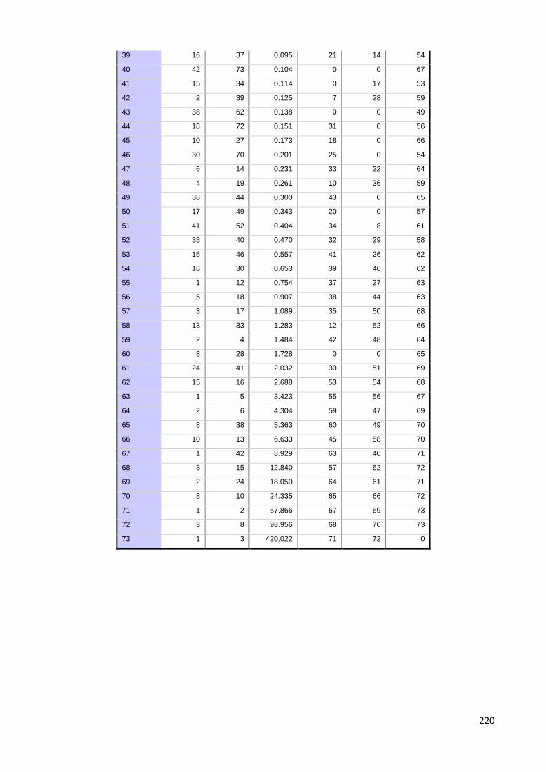
220

39 16 37 0.095 21 14 54

40 42 73 0.104 0 0 67

41 15 34 0.114 0 17 53

42 2 39 0.125 7 28 59

43 38 62 0.138 0 0 49

44 18 72 0.151 31 0 56

45 10 27 0.173 18 0 66

46 30 70 0.201 25 0 54

47 6 14 0.231 33 22 64

48 4 19 0.261 10 36 59

49 38 44 0.300 43 0 65

50 17 49 0.343 20 0 57

51 41 52 0.404 34 8 61

52 33 40 0.470 32 29 58

53 15 46 0.557 41 26 62

54 16 30 0.653 39 46 62

55 1 12 0.754 37 27 63

56 5 18 0.907 38 44 63

57 3 17 1.089 35 50 68

58 13 33 1.283 12 52 66

59 2 4 1.484 42 48 64

60 8 28 1.728 0 0 65

61 24 41 2.032 30 51 69

62 15 16 2.688 53 54 68

63 1 5 3.423 55 56 67

64 2 6 4.304 59 47 69

65 8 38 5.363 60 49 70

66 10 13 6.633 45 58 70

67 1 42 8.929 63 40 71

68 3 15 12.840 57 62 72

69 2 24 18.050 64 61 71

70 8 10 24.335 65 66 72

71 1 2 57.866 67 69 73

72 3 8 98.956 68 70 73

73 1 3 420.022 71 72 0

221

Figure C1: Graphical presentation of the Agglomeration Schedule

Table C2: Total Variance explained by each factor

0.000

50.000

100.000

150.000

200.000

250.000

300.000

350.000

400.000

450.000

1 5 9 13 17 21 25 29 33 37 41 45 49 53 57 61 65 69 73

Series1

Total Variance Explained Total Variance Explained

componant Initial Eigenvalues Rotation Sums of Squared Loadings ComponentRotation Sums of Squared Loadings

Total % of Variance Cumulative % Total % of Variance Cumulative %

1 5.534 32.552 32.552 4.175 24.557 1 24.557

2 2.605 15.322 47.874 2.995 17.618 2 42.175

3 2.153 12.667 60.541 2.195 12.912 3 55.087

4 1.584 9.318 69.86 2.074 12.201 4 67.289

5 0.988 5.811 75.671 1.425 8.382 5 75.671

6 0.95 5.59 81.261 6

7 0.714 4.202 85.463 7

8 0.541 3.185 88.648 8

9 0.452 2.659 91.308 9

10 0.328 1.929 93.236 10

11 0.263 1.544 94.781 11

12 0.228 1.343 96.123 12

13 0.196 1.153 97.276 13

14 0.157 0.926 98.202 14

15 0.125 0.734 98.936 15

16 0.095 0.561 99.498 16

17 0.085 0.502 100 17

222

Table C3: Rescaled factor scores

F1 F2 F3 F4 F5 Total

Aurukun (S) 0.0317632 0.2221594 0.0332801 0.0379672 0.0187984 0.3439683

Balonne (S) 0.1826582 0.118254 0.3874099 0.4027926 0.5885901 1.6797048

Banana (S) 0.415964 0.0891038 0.6704293 0.5908951 0.6655328 2.431925

Barcaldine (R) 0.1717181 0.1044173 0.2821096 0.4078515 0.6100442 1.5761407

Barcoo (S) 0.1323366 0.0989269 0.1837807 0.3488837 0.508489 1.2724169

Blackall Tambo (R) 0.1438728 0.0507543 0.2391977 0.4220411 0.6285146 1.4843805

Boulia (S) 0.1123179 0.0919732 0.1698035 0.3079732 0.4142482 1.096316

Brisbane (C) 0.2823426 0.0660731 0.343096 1 1 2.6915116

Bulloo (S) 0.1446022 0.1594955 0.2115666 0.3778529 0.562684 1.4562011

Bundaberg (R) 0.3390066 0.0976154 0.4617352 0.5823266 0.7504249 2.2311086

Burdekin (S) 0.1826418 0.1501765 0.2613251 0.4493693 0.6372698 1.6807825

Burke (S) 0.1139916 0.201162 0.1539283 0.1970509 0.2996172 0.96575

Cairns (R) 0.5267408 0.2718317 0.4149504 0.6668525 0.8177738 2.6981493

Carpentaria (S) 0.1531557 0.368661 0.2677429 0.2921648 0.4273925 1.5091169

Cassowary Coast (R) 0.4681786 0.3214454 0.3649338 0.5371232 0.6815551 2.3732361

Central Highlands (R) 0.5167105 0.1926293 1 0.6066842 0.6291666 2.9451905

Charters Towers (R) 0.2891647 0.2789201 0.313978 0.4400682 0.6627125 1.9848434

Cherbourg (S) 0.0157381 0.0732234 0.0313477 0.0584259 0.0830645 0.2617995

Cloncurry (S) 0.1202716 0.0457856 0.2053402 0.3778324 0.5570658 1.3062955

Cook (S) 0.6745731 1 0.3975216 0.3514012 0.1073132 2.530809

Croydon (S) 0.0934223 0.0621226 0.149181 0.2885632 0.4018339 0.995123

Diamantina (S) 0.2065666 0.3301066 0.2282306 0.3643182 0.506228 1.6354499

Doomadgee (S) 0.0515066 0.0596295 0.1027193 0.1962248 0.2859455 0.6960257

Etheridge (S) 0.2169129 0.155543 0.218135 0.3294779 0.3759669 1.2960357

Flinders (S) 0.1462507 0.0634394 0.2164236 0.3984827 0.593374 1.4179704

Fraser Coast (R) 0.4269996 0.1294314 0.5367611 0.629793 0.7367385 2.4597236

Gladstone (R) 0.546301 0.2301299 0.643654 0.6916409 0.8148562 2.926582

Gold Coast (C) 0.3484333 0.0943215 0.4289211 0.8164727 0.8917941 2.5799427

Goondiwindi (R) 0.2522245 0.0469742 0.553996 0.4659947 0.5566135 1.8758029

Gympie (R) 0.4971314 0.1375433 0.5921008 0.6347262 0.699255 2.5607567

Hinchinbrook (S) 0.2077632 0.1101781 0.2713062 0.4504371 0.6109323 1.6506169

Hope Vale (S) 0.0711878 0.0790294 0.1149111 0.2148096 0.3051961 0.7851339

Ipswich (C) 0.1777797 0.0178886 0.3164336 0.599451 0.773249 1.8848019

Isaac (R) 0.4929092 0.1938148 0.9513196 0.6472226 0.6850684 2.9703346

Kowanyama (S) 0.0406021 0.1575108 0.0414907 0.0821488 0.0985376 0.42029

Lockhart River (S) 0.0497613 0.1041692 0.0636788 0.124212 0.1700886 0.5119098

Lockyer Valley (R) 0.2601358 0.0827185 0.3232429 0.520877 0.6839799 1.8709541

Logan (C) 0.2440382 0.0477683 0.3561755 0.6965782 0.8114704 2.1560305

Longreach (R) 0.1620018 0.0531777 0.2318244 0.4456588 0.6928594 1.5855222

Mackay (R) 0.581578 0.2512692 0.5589139 0.6986771 0.8574589 2.9478972

McKinlay (S) 0.1267076 0.0351982 0.2305709 0.4224369 0.6229766 1.4378903

Mapoon (S) 0.0729645 0.0704098 0.1332894 0.2548666 0.3623429 0.8938732

223

Maranoa (R) 0.3490139 0.0524426 0.6372385 0.536161 0.6200278 2.1948837

Moreton Bay (R) 0.4299372 0.0902274 0.5298221 0.8219803 0.8402445 2.7122115

Mornington (S) 0.0354201 0.0810109 0.0706642 0.1315393 0.2003368 0.5189713

Mount Isa (C) 0.1779948 0.0989623 0.2483002 0.4396523 0.6536055 1.6185152

Murweh (S) 0.157876 0.0663619 0.271949 0.410711 0.5850906 1.4919884

Napranum (S) 0 0.1017027 0 0 0 0.1017027

North Burnett (R) 0.4891593 0.1030633 0.6393706 0.5399513 0.5133364 2.2848809 Northern Peninsula Area (R) 0.0589913 0.0629334 0.1141969 0.2181506 0.3111978 0.76547

Palm Island (S) 0.17564 0 0.3354115 0.631583 0.9044601 2.0470946

Paroo (S) 0.1630541 0.150911 0.1707999 0.3295502 0.4663932 1.2807084

Pormpuraaw (S) 0.0491299 0.1223738 0.0741918 0.149549 0.2222697 0.6175143

Quilpie (S) 0.1628257 0.0992057 0.2153085 0.4142263 0.6142364 1.5058027

Redland (C) 0.260368 0.0564954 0.3793157 0.6777231 0.8312124 2.2051146

Richmond (S) 0.1097333 0.0353307 0.1991245 0.3810543 0.568496 1.2937387

Rockhampton (R) 0.4842551 0.2686626 0.5202369 0.6366734 0.781438 2.691266

Scenic Rim (R) 0.2677208 0.0738369 0.349395 0.5557799 0.723746 1.9704786

Somerset (R) 0.4036742 0.1112665 0.5154644 0.5840133 0.7141149 2.3285333

South Burnett (R) 0.2820198 0.0519097 0.4571386 0.5213993 0.6286747 1.9411421

Southern Downs (R) 0.3647804 0.0914521 0.4127847 0.5380493 0.6413318 2.0483983

Sunshine Coast (R) 0.9068779 0.3028235 0.8011037 0.9334187 0.9115015 3.8557254

Tablelands (R) 1 0.5676021 0.7357093 0.7081298 0.5556295 3.5670706

Toowoomba (R) 0.3353533 0.0634516 0.6428513 0.6146171 0.6587321 2.3150054

Torres (S) 0.1208948 0.1042725 0.1815432 0.3291678 0.4665435 1.2024218

Torres Strait Island (R) 0.057676 0.0557488 0.1142859 0.2190444 0.3172782 0.7640333

Townsville (C) 0.3134155 0.1610542 0.3744848 0.6407807 0.8688677 2.3586027

Weipa (T) 0.1411941 0.0139323 0.269059 0.5295051 0.7301424 1.6838328

Western Downs (R) 0.3952347 0.0496537 0.8872109 0.5593135 0.5742511 2.465664

Whitsunday (R) 0.3601743 0.2786528 0.4095233 0.5199407 0.6806148 2.248906

Winton (S) 0.1342132 0.0476413 0.2110523 0.3755997 0.5671243 1.3356308

Woorabinda (S) 0.0588924 0.0605382 0.1028073 0.1653835 0.2247325 0.6123539

Wujal Wujal (S) 0.0705845 0.0468572 0.1362148 0.2630076 0.3786207 0.8952849

Yarrabah (S) 0.0474453 0.0876139 0.0667157 0.1088275 0.1476359 0.4582383

natural amenities and tourism employment: a spatial analysis

Documents