natural resources and economic growth: some theory - citeseer

ANNALS OF ECONOMICS AND FINANCE 10-2, 367–389 (2009)

Natural Resources and Economic Growth: Some Theory and

Evidence*

Dustin Chambers

Department of Economics and Finance, Salisbury University, 1101 Camden Ave.Salisbury, MD 21801

E-mail: [email protected]

and

Jang-Ting Guo

Department of Economics, 4123 Sproul Hall, University of California, Riverside,CA, 92521

E-mail: [email protected]

We develop a one-sector endogenous growth model in which renewable nat-ural resources are both a factor of production and measure of environmentalquality. Along the balanced growth path, sustained economic growth and anon-deteriorating environment are shown to coexist. Moreover, steady-stateeconomic growth and natural-resource utilization are positively related. Em-pirically, a cross-country growth regression that includes a broad measure ofproductive natural resources — the Ecological Footprint — provides strongsupport. Our estimation results also suggest conservation costs are minimal,and growth strategies based on greater physical capital formation and tradeopenness outperform those relying on more intensive utilization of the envi-ronment.

Key Words: Natural resources; Endogenous growth; Ecological footprint.JEL Classification Numbers: O41, Q21, Q56.

1. INTRODUCTION

In response to high energy prices and the OPEC oil embargo duringthe 1970’s, economists began to systematically examine the growth ef-

* We are indebted to Ken Baerenklau, Shu-Hua Chen, Keith Knapp, and RichardSuen for helpful discussions and comments. Part of this research was conducted whileGuo was a visiting research fellow at the Institute of Economics, Academia Sinica, whosehospitality is greatly appreciated. Of course, all remaining errors are our own.

3671529-7373/2009

All rights of reproduction in any form reserved.

368 DUSTIN CHAMBERS AND JANG-TING GUO

fects of non-renewable natural resources within dynamic general equilib-rium macroeconomic models. For example, using an exogenous-growthframework, Solow (1974) and Stiglitz (1974) show that sustained economicgrowth is possible so long as the reproducible factor of production (physi-cal capital) can be substituted for exhaustible natural resources along theeconomy’s balanced growth path.1 This finding, while unquestionably es-sential, is somewhat restrictive in scope in that it ignores the impact ofeconomic activities on the quality and state of the environment. As aresult, economists began to broaden their focus and investigate the inter-relations between economic growth and pollution emissions in the 1990’s.Specifically, Stokey (1998) finds that continuing growth is possible despiteever tightening pollution restrictions that are met with costly abatement.More recently, Brock and Taylor (2005) demonstrate the co-existence ofsustained economic growth and zero net pollution emissions (dubbed the“Kindergarten Rule”) within an endogenous growth model in which theabatement technology improves through learning-by-doing. Although thislatter branch of the literature implicitly discusses the relationship betweeneconomic development and environmental quality through the narrow lensof pollution, it neglects the additional role that natural resources play inthe production of GDP and hence long-run economic growth. Motivated bythis gap, we develop a stylized one-sector endogenous growth model thatcaptures the environment’s dual roles as (i) a provider of factors of produc-tion, and (ii) a stock of renewable natural resources that accumulates overtime to preserve environmental quality as GDP continues to grow. Ourmain finding is that in the long run, the economy’s output growth rate ispositively related to the steady-state level of utilized natural resources. Inaddition, a panel cross-country growth regression, which includes a broadmeasure of productive natural resources, provides strong empirical supportfor this theoretical prediction.

The results of Solow (1974), Stiglitz (1974), and Stokey (1998), amongothers, together suggest that sustained economic growth is possible despitelimitations on the productive availability of exhaustible natural resources,and that additional costs and restrictions associated with preserving envi-ronmental quality are not an insurmountable impediment to growth. Bycontrast, this paper focuses on the feasibility of a balanced-growth equilib-rium with non-deteriorating environmental quality in a canonical one-sectorendogenous growth model with renewable natural resources. In our modeleconomy, households live forever, provide fixed labor supply and deriveutility from consumption goods. On the production side, a continuum ofidentical, competitive firms produce output using natural resources, which

1Suzuki (1976) finds that continuing output growth can arise within environmentalendogenous growth models as well.

NATURAL RESOURCES AND ECONOMIC GROWTH 369

are assumed to regenerate at a constant rate over time, as a factor of pro-duction. The economy’s aggregate production function displays increasingreturns-to-scale because of the presence of productive externalities gener-ated by capital inputs. We show that along the balanced growth path(BGP), output, consumption, and physical capital all grow at a commonpositive rate, whereas the stock of total natural resources and the level ofnatural resources allocated to the firms’ production process maintain theirrespective steady-state values.2 It follows that the quantity of utilized nat-ural resources per unit of GDP steadily declines in the economy’s BGPequilibrium, a result that is also echoed in Solow (1974), Stiglitz (1974),and Stokey (1998) under non-renewable resources. Furthermore, we findthat an increase of natural-resource utilization in production will raise theBGP’s output growth rate.

Next, to empirically verify our main theoretical finding, we incorporatean inclusive measure of productive natural resources — the Ecological Foot-print (EF) — into Barro’s (1991) panel cross-country growth regressionmodel. Formally speaking, natural capital includes all the productive re-sources that can be extracted from the earth, as well as all the biologicalprocesses and services that facilitate life such as the absorption of waste orthe conversion of carbon-dioxide into oxygen. The EF series is based onthis broader concept of natural capital. As described in Rees (1992) andWackernagel and Rees (1996), the EF variable systematically measuresthe quantity of renewable natural resources and life-facilitating servicesdemanded by each nation.3 In order to overcome the inherent problemof aggregating over many disparate measures, the Ecological Footprint isconstructed by first converting an exhaustive and comprehensive list of re-newable natural resources and life-support services into standardized unitsof land area called global hectares. The resulting quantity, expressed inper-capita terms, offers a standardized measure of the land needed to sup-port an average person’s consumption expenditures (based on the country’scurrent level of per-capita income), and to facilitate ecologically necessarylife-facilitating services. To our knowledge, the EF series is the best avail-able aggregate proxy for natural-resource utilization in the economy’s pro-duction process for a large panel of countries.

In addition to the Ecological Footprint, our dataset consists of a broadinternational panel that includes 5-year growth spells of output, togetherwith some standard conditioning variables such as initial per-capita GDP,an educational attainment proxy for human capital, government and invest-

2See Smulders (1999) for a survey of other mechanisms that also demonstrate thecompatibility of continuing output growth and environmental preservation within thecontext of endogenous growth models.

3The Ecological Footprint does not include measures of mineral deposits extracted ina given year.


ment’s shares of output, and trade openness. In order to obtain unbiasedestimates from our dynamic panel regressions, Arellano and Bond’s (1991)two-step GMM estimation procedure is employed. It is first shown that ourempirical model passes the necessary specification tests whereby no secondor higher-order serial correlations in the estimation residuals are present.We then show that the estimated coefficient on the Ecological Footprint ispositive and statistically significant at the 1% level. This estimation resultprovides strong empirical support for the key prediction of our theoreticalmodel, that is, more intensive utilization of natural resources in productionleads to an increase in the economy’s output growth rate. Moreover, thesigns and statistical significance of the remaining regressors are generallyin-line with neoclassical growth theory and previous empirical studies. Wealso perform a sensitivity analysis on our benchmark econometric specifi-cation by leaving out a variety of combinations of components from thefootprint measure, or by including separate components of the EF series.As it turns out, the results from these alternative estimations broadly sup-port our main empirical finding that natural-resource utilization positivelycontributes to future economic growth.

The remainder of this paper is organized as follows. Section 2 describesthe theoretical model and analyzes the equilibrium conditions for the econ-omy’s balanced growth path. Section 3 employs an international paneldataset that includes the Ecological Footprint to empirically verify ourmain theoretical findings. Section 4 concludes.

2. THE THEORETICAL MODEL

To provide the simplest possible analytical framework for motivatingour empirical study, we modify Smulders’ (1999, section 2.2) highly styl-ized one-sector environmental endogenous growth model in which the rep-resentative household lives forever, provides fixed labor supply, and de-rives utility from consumption goods. The economy’s social technologyexhibits increasing returns-to-scale because of the presence of productiveexternalities generated by capital inputs. For expositional simplicity, andto maintain consistency with the subsequent empirical work that employsthe Ecological Footprint to measure environmental utilization, we assumethat all natural resources are renewable (such as a forest or fishery) inour theoretical model. Moreover, some of the natural resources are usedin the firm’s production function to capture the environment’s productivevalue. Our main objective is to explore the interrelations between the out-put growth rate and environmental quality along the economy’s balancedgrowth path.


2.1. FirmsThere is a continuum of identical, competitive firms in the economy, with

the total number normalized to one. Each firm produces output Yt usinga constant returns-to-scale Cobb-Douglas production function

Yt = Kαt H1−α

t Xt, 0 < α < 1, (1)

where Kt and Ht are physical capital and harvested/utilized natural re-sources (or natural capital), respectively, and Xt represents productive ex-ternalities that are taken as given by individual firms.4 In addition, Xt ispostulated to take the form

Xt = AK1−α

t , A > 0, (2)

where Kt denotes the economy-wide average level of the capital stock. Ina symmetric equilibrium, all firms take the same actions such that Kt =Kt. Hence, (2) can be substituted into (1) to obtain the following socialproduction function that displays increasing returns-to-scale:

Yt = AKtH1−αt . (3)

Under the assumption that factor markets are perfectly competitive, thefirst-order conditions for the firm’s profit maximization problem are givenby

rt = αYt

Kt, (4)

pt = (1− α)Yt

Ht, (5)

where rt is the capital rental rate and pt is the real price paid to utilizednatural resources.

2.2. HouseholdsThe economy is populated by a unit measure of identical infinitely-lived

households, each has perfect foresight and maximizes a discounted streamof utilities over its lifetime∫ ∞

0

C1−σt − 11− σ

e−ρtdt, σ > 0, σ 6= 1, (6)

4By contrast, Sumlders (1999) postulates that it is the stock of a broadly-definedcapital, which includes physical capital as well as man-made knowledge (i.e. humancapital), that enters the firm’s production technology (1). None of our theoretical resultsare affected by this difference of modeling assumption.


where Ct is the individual household’s consumption, ρ ∈ (0, 1) is the sub-jective discount rate, and σ is the inverse of the intertemporal elasticity ofsubstitution in consumption.

The budget constraint faced by the representative household is

Ct + Kt + δKt = rtKt + ptHt, K0 > 0 given, (7)

where δ ∈ [0, 1] is the capital depreciation rate. As is commonly specifiedin the environmental macroeconomics literature (see, for example, Smul-ders (1999) and references therein), the economy’s ecological process or thelaw of motion for total renewable resources (as a proxy for environmentalquality) Nt is given by

Nt = f(Nt)Nt −Ht, N0 > 0 given, (8)

where f(Nt) is the regeneration function that is often assumed to be strictlyincreasing in Nt. Without loss of any generality, we postulate that the rateof natural regeneration is independent of the environmental state, specif-ically f(Nt) = θ > 0.5 On the other hand, as pointed out by Smulders(1999, p. 612), Ht represents not only the extraction of natural resources,but also the disposal of wastes (i.e. pollution) because both activities re-duce the environment’s absorption capacity represented by f(Nt)Nt.

The first-order conditions for the representative household’s dynamicoptimization problem are

C−σt = λKt

, (9)λKt

(rt − δ) = −λKt+ ρλKt

, (10)θλNt

= −λNt+ ρλNt

, (11)λKt

pt = λNt, (12)

limt→∞

λKtKte

−ρt = 0, (13)

limt→∞

λNtNte−ρt = 0, (14)

where λKtand λNt

are shadow prices (or utility values) of capital stockand natural resources, respectively. Equation (9) states that the marginalbenefit of consumption equals its marginal cost, which is the marginalutility of having an additional unit of physical capital. In addition, (10) and(11) are standard Euler equations that govern the evolution of Kt and Nt

over time. Equation (12) shows that the firm utilizes natural resources to

5We also consider the formulation in which only the non-utilized natural resourcesare allowed to regenerate. In this case, the accumulation equation (8) becomes Nt =θNt − (1 + θ)Ht. It turns out that all our theoretical results are qualitatively robust tothis modification.


the point where the marginal value of more output is equal to the marginalcost of resource depletion. Finally, (13) and (14) are the transversalityconditions (TVC).

2.3. Balanced Growth PathIn light of the household’s CRRA utility formulation (6), together with

the linearity of physical capital in the aggregate technology (3), the econ-omy exhibits sustained endogenous growth whereby output, consumption,and physical capital all display a common, positive constant growth ratedenoted by g. Moreover, the regeneration/depletion equation (8) impliesthat in the long run (or in an ecological equilibrium defined as Nt = 0),total and utilized natural resources will reach their respective steady-statelevels, N∗ and H∗. This in turn imposes a sustainable long-run environ-mental quality constraint, as in Solow (1974), Stiglitz (1974), and Stokey(1998) under exhaustible natural resources, where a constant level of pol-lution exactly matches the environment’s absorption capacity.

To derive a balanced growth path (BGP), we first make the variabletransformation Xt ≡ Ct

Kt, and re-express the model’s equilibrium conditions

as the following autonomous differential equations:

Xt

Xt=

αAH1−αt − δ − ρ

σ−AH1−α

t + Xt + δ, (15)

Ht

Ht=

1α

[A(1− α)H1−α

t −Xt + θ], (16)

Nt = θNt −Ht. (17)

Given the above dynamical system (15)-(17), the balanced-growth equi-librium is characterized by a triplet of positive real numbers (X∗,H∗, N∗)that satisfy the condition Xt = Ht = Nt = 0. It is straightforward to showthat our model economy exhibits a unique balanced growth path alongwhich the utilized natural resource maintains its steady-state level

H∗ =[σθ − [ρ− (σ − 1)δ]

αA(σ − 1)

]1/(1−α)

, (18)

which in turn leads to the expressions for X∗ and N∗ as follows:

X∗ = A(1− α)(H∗)1−α + θ and N∗ =H∗

θ. (19)

With (18) and (19), it follows that the common (positive) rate of economicgrowth g is given by

g =θ − ρ

σ − 1or g = αA(H∗)1−α − θ − ρ. (20)


As a result, the BGP’s growth rate ceteris paribus is positively relatedto the steady-state level of utilized natural resources.6 That is, a higher(lower) usage of services from the environment in production will raise(reduce) the economy’s rate of growth in output, consumption, and physicalcapital. Moreover, the quantity of utilized natural resources per unit ofGDP steadily declines along the economy’s balanced growth path, a resultthat is also echoed in Solow (1974), Stiglitz (1974), and Stokey (1998),among many others.

3. THE EMPIRICAL MODEL

There are two interesting implications that follow from the above theoret-ical model. First, as mentioned earlier, the BGP’s output growth rate riseswith the productive utilization of natural resources ∂g

∂H∗ > 0. Second, theeconomy’s long-run rate of economic growth increases with the reproduc-tion rate of natural resources ∂g

∂θ > 0. The latter implication is difficult toverify empirically because of the need to access data on the stock of naturalresources, whereas the former is more easily testable given that it requiresthe flow of natural resources used in production. As a result, we restrictour empirical analyses to the output-growth effect of natural-resource uti-lization. In particular, we incorporate natural-resource usage into Barro’s(1991) specification and examine the following panel cross-country growthregression model:

growthit+1 = β1incomeit + β2educationit + β3govit + β4invit

+β5tradeit + β6footprintit + αi + ηt + εit+1 (21)

where the dependent variable (growthit+1) measures the average annualgrowth in real GDP per capita of country i over the next 5-year period(between t and t + 1). To account for conditional convergence, our modelincludes incomeit, which is the natural log of PPP-adjusted, chain-weightedper-capital GDP at period t. Human capital is controlled by way of theproxy educationit, which equals the average years of education for the entirepopulation aged 15 and above. To account for differences in fiscal policiesacross countries, we include govit, which measures public expenditures ongoods and services relative to GDP (i.e. Git/Yit), as a conditioning vari-able. To control for the rate of capital formation, the investment share inoutput (i.e. Iit/Yit), denoted as invit, is also included. The openness ofa nation is captured by tradeit, which is the ratio of total trade to GDP,i.e. (IMit + EXit)/Yit. To control for the natural-resource utilization inproduction, we include footprintit, which equals the natural log of the per-

6To ensure that the BGP’s output growth rate g is positive, we impose the followingparametric restriction: θ > (<)ρ when σ > (<)1.


capita quantity of renewable natural resources, in our panel estimation.Finally, αi is a country-specific effect, ηt is a period-specific effect, andεit+1 is an i.i.d. stochastic shock with zero mean and standard deviationσ2

ε .

3.1. The DataOur international panel dataset is constructed from three sources. Out-

put growth, income, government and investment’s shares of GDP, and tradeopenness are taken from the Penn World Table v. 6.2 (Heston, Summers,and Aten, 2006). These variables are expressed as percentages with theexception of income, which is expressed (prior to taking the natural log) inconstant (2000) international dollars ($I). The education series comes fromBarro and Lee (2000), and measures the average years of schooling for theentire population aged 15 and above. Finally, the natural-resource series— the Ecological Footprint (EF) — is obtained from the Global FootprintNetwork (2005).7 This variable measures the quantity of renewable natu-ral resources, in standardized global hectares (gha), needed to produce anation’s current level of per-capita consumption. Specifically, the EF seriesis equal to the sum of seven underlying components: the land required toproduce crops for both human and animal consumption (henceforth de-noted as “crops”); the land required to maintain pasture-grazing animals(denoted as “pasture”); the land required to harvest forest products, whichis sub-divided between wood for fuel (denoted as “fuelwood”) and all otherforest products (denoted as “timber”); the freshwater and oceanic surfacearea required to produce fishing harvests (denoted as “fish”); the land re-quired to sequester carbon dioxide emissions from the burning of fossil fuels(denoted as “CO2”); and the land that has been developed for commercialand residential uses (denoted as “built”). Since the value of permanentimprovements to land and to the structures placed on land are generallyconsidered as parts of a nation’s stock of physical capital, including them ina flow measurement of renewable resources is not appropriate. Therefore,we remove the developed-land component (i.e. “built”) from the total EFseries in our empirical estimations.8

Although the Ecological Footprint possesses the obvious attractivenessof being a single statistic designed to capture the aggregate utilization ofrenewable natural resources, it suffers the same drawback of any aggre-gated measure: strong assumptions are required in its construction. Forexample, it lumps together the input and environmental effects, i.e. un-wanted outputs like waste and the damage from CO2; and it confuses flow

7See Haberl, Erb, and Krausmann (2001) for a good introduction on how ecologicalfootprints are calculated.

8The nuclear power component (which is a sub-component of the “CO2” series) isremoved from the footprint indicator used in the subsequent estimations as well.


versus stock effects, e.g. the cost of cleaning up soils is imputed. Moreover,Ayers (2000) takes issue with the underlying assumptions with regard tothe carbon dioxide sequestering and the conversion of energy consumptioninto land usage areas. Van Kooten and Bulte (2000) highlight the EF in-ability to tackle important ecological topics such as soil erosion and carbonabsorption. In order to alleviate these concerns, we perform robustnesschecks (in section 3.5) — leaving out a variety of combinations of compo-nents from the footprint measure, or including separate components of theEF indicator — on our benchmark empirical model that uses the modified(six-component) EF series as a regressor.

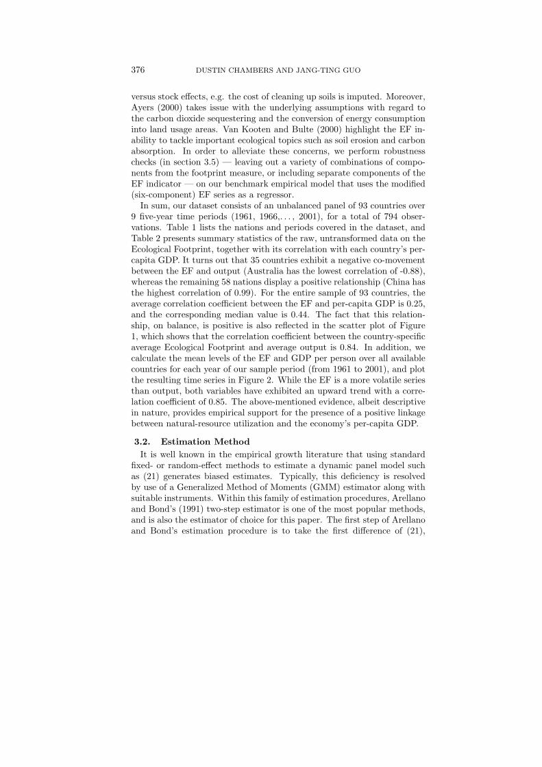
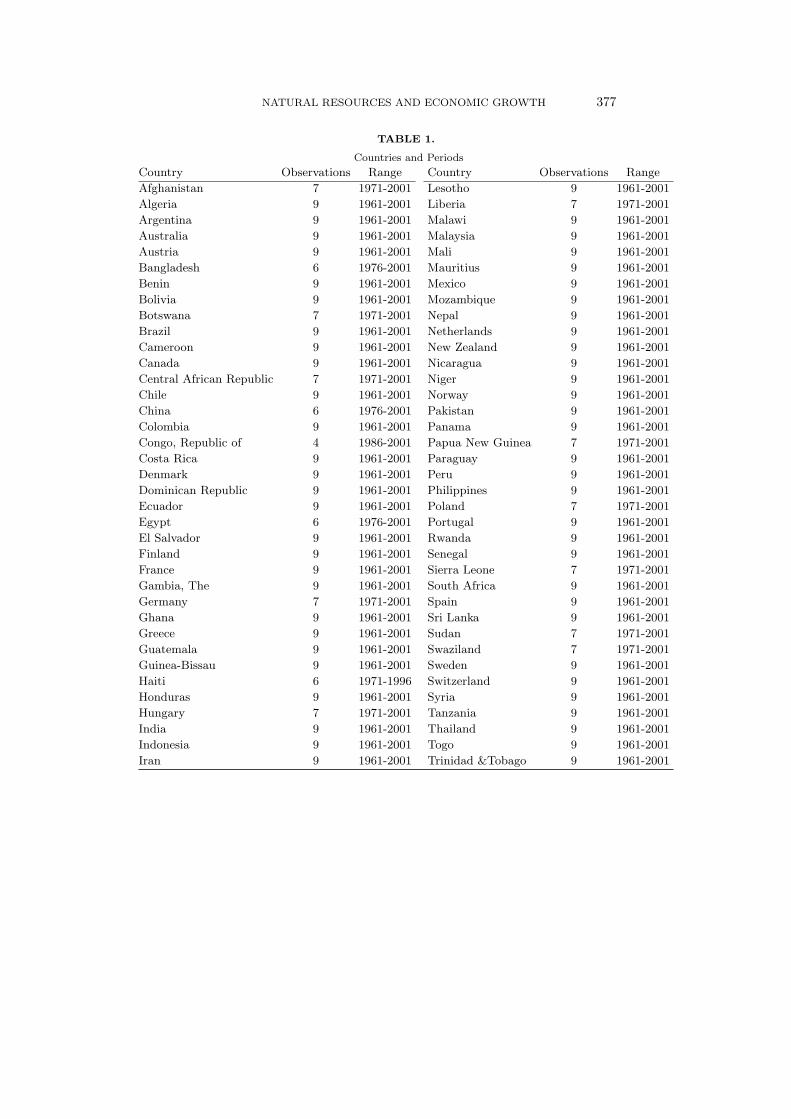
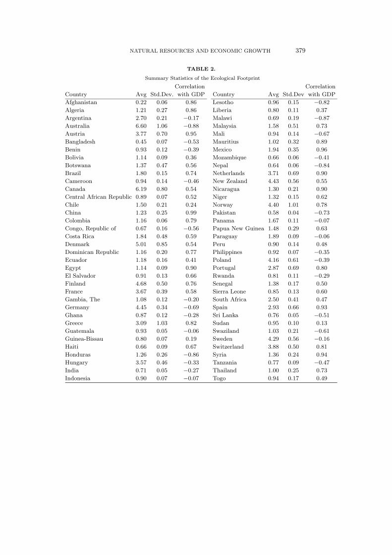
In sum, our dataset consists of an unbalanced panel of 93 countries over9 five-year time periods (1961, 1966,. . . , 2001), for a total of 794 obser-vations. Table 1 lists the nations and periods covered in the dataset, andTable 2 presents summary statistics of the raw, untransformed data on theEcological Footprint, together with its correlation with each country’s per-capita GDP. It turns out that 35 countries exhibit a negative co-movementbetween the EF and output (Australia has the lowest correlation of -0.88),whereas the remaining 58 nations display a positive relationship (China hasthe highest correlation of 0.99). For the entire sample of 93 countries, theaverage correlation coefficient between the EF and per-capita GDP is 0.25,and the corresponding median value is 0.44. The fact that this relation-ship, on balance, is positive is also reflected in the scatter plot of Figure1, which shows that the correlation coefficient between the country-specificaverage Ecological Footprint and average output is 0.84. In addition, wecalculate the mean levels of the EF and GDP per person over all availablecountries for each year of our sample period (from 1961 to 2001), and plotthe resulting time series in Figure 2. While the EF is a more volatile seriesthan output, both variables have exhibited an upward trend with a corre-lation coefficient of 0.85. The above-mentioned evidence, albeit descriptivein nature, provides empirical support for the presence of a positive linkagebetween natural-resource utilization and the economy’s per-capita GDP.

3.2. Estimation MethodIt is well known in the empirical growth literature that using standard

fixed- or random-effect methods to estimate a dynamic panel model suchas (21) generates biased estimates. Typically, this deficiency is resolvedby use of a Generalized Method of Moments (GMM) estimator along withsuitable instruments. Within this family of estimation procedures, Arellanoand Bond’s (1991) two-step estimator is one of the most popular methods,and is also the estimator of choice for this paper. The first step of Arellanoand Bond’s estimation procedure is to take the first difference of (21),


TABLE 1.

Countries and Periods

Country Observations Range Country Observations Range

Afghanistan 7 1971-2001 Lesotho 9 1961-2001

Algeria 9 1961-2001 Liberia 7 1971-2001

Argentina 9 1961-2001 Malawi 9 1961-2001

Australia 9 1961-2001 Malaysia 9 1961-2001

Austria 9 1961-2001 Mali 9 1961-2001

Bangladesh 6 1976-2001 Mauritius 9 1961-2001

Benin 9 1961-2001 Mexico 9 1961-2001

Bolivia 9 1961-2001 Mozambique 9 1961-2001

Botswana 7 1971-2001 Nepal 9 1961-2001

Brazil 9 1961-2001 Netherlands 9 1961-2001

Cameroon 9 1961-2001 New Zealand 9 1961-2001

Canada 9 1961-2001 Nicaragua 9 1961-2001

Central African Republic 7 1971-2001 Niger 9 1961-2001

Chile 9 1961-2001 Norway 9 1961-2001

China 6 1976-2001 Pakistan 9 1961-2001

Colombia 9 1961-2001 Panama 9 1961-2001

Congo, Republic of 4 1986-2001 Papua New Guinea 7 1971-2001

Costa Rica 9 1961-2001 Paraguay 9 1961-2001

Denmark 9 1961-2001 Peru 9 1961-2001

Dominican Republic 9 1961-2001 Philippines 9 1961-2001

Ecuador 9 1961-2001 Poland 7 1971-2001

Egypt 6 1976-2001 Portugal 9 1961-2001

El Salvador 9 1961-2001 Rwanda 9 1961-2001

Finland 9 1961-2001 Senegal 9 1961-2001

France 9 1961-2001 Sierra Leone 7 1971-2001

Gambia, The 9 1961-2001 South Africa 9 1961-2001

Germany 7 1971-2001 Spain 9 1961-2001

Ghana 9 1961-2001 Sri Lanka 9 1961-2001

Greece 9 1961-2001 Sudan 7 1971-2001

Guatemala 9 1961-2001 Swaziland 7 1971-2001

Guinea-Bissau 9 1961-2001 Sweden 9 1961-2001

Haiti 6 1971-1996 Switzerland 9 1961-2001

Honduras 9 1961-2001 Syria 9 1961-2001

Hungary 7 1971-2001 Tanzania 9 1961-2001

India 9 1961-2001 Thailand 9 1961-2001

Indonesia 9 1961-2001 Togo 9 1961-2001

Iran 9 1961-2001 Trinidad &Tobago 9 1961-2001


Country Observations Range Country Observations Range

Iraq 7 1971-2001 Tunisia 9 1961-2001

Ireland 9 1961-2001 Turkey 9 1961-2001

Israel 9 1961-2001 Uganda 9 1961-2001

Italy 9 1961-2001 United Kingdom 9 1961-2001

Jamaica 9 1961-2001 United States 9 1961-2001

Japan 9 1961-2001 Uruguay 9 1961-2001

Jordan 9 1961-2001 Venezuela 9 1961-2001

Kenya 9 1961-2001 Zambia 9 1961-2001

Korea, Republic of 9 1961-2001 Zimbabwe 9 1961-2001

Kuwait 7 1971-2001

FIG. 1. Scatter Plot of Real Output and the Ecological Footprint

!Note: Diagram includes 93 observations, each consisting of

country-specific averages over all available time periods.

which, after some algebraic manipulation, can be expressed as (22)

∆incomeit+1 = (1 + β1)∆incomeit + β2∆educationit + β3∆govit + β4∆invit

+β5∆tradeit + β6∆footprintit + ∆ηt + ∆εit+1 (22)


TABLE 2.

Summary Statistics of the Ecological Footprint

Correlation Correlation

Country Avg Std.Dev. with GDP Country Avg Std.Dev with GDP

Afghanistan 0.22 0.06 0.86 Lesotho 0.96 0.15 −0.82

Algeria 1.21 0.27 0.86 Liberia 0.80 0.11 0.37

Argentina 2.70 0.21 −0.17 Malawi 0.69 0.19 −0.87

Australia 6.60 1.06 −0.88 Malaysia 1.58 0.51 0.73

Austria 3.77 0.70 0.95 Mali 0.94 0.14 −0.67

Bangladesh 0.45 0.07 −0.53 Mauritius 1.02 0.32 0.89

Benin 0.93 0.12 −0.39 Mexico 1.94 0.35 0.96

Bolivia 1.14 0.09 0.36 Mozambique 0.66 0.06 −0.41

Botswana 1.37 0.47 0.56 Nepal 0.64 0.06 −0.84

Brazil 1.80 0.15 0.74 Netherlands 3.71 0.69 0.90

Cameroon 0.94 0.14 −0.46 New Zealand 4.43 0.56 0.55

Canada 6.19 0.80 0.54 Nicaragua 1.30 0.21 0.90

Central African Republic 0.89 0.07 0.52 Niger 1.32 0.15 0.62

Chile 1.50 0.21 0.24 Norway 4.40 1.01 0.78

China 1.23 0.25 0.99 Pakistan 0.58 0.04 −0.73

Colombia 1.16 0.06 0.79 Panama 1.67 0.11 −0.07

Congo, Republic of 0.67 0.16 −0.56 Papua New Guinea 1.48 0.29 0.63

Costa Rica 1.84 0.48 0.59 Paraguay 1.89 0.09 −0.06

Denmark 5.01 0.85 0.54 Peru 0.90 0.14 0.48

Dominican Republic 1.16 0.20 0.77 Philippines 0.92 0.07 −0.35

Ecuador 1.18 0.16 0.41 Poland 4.16 0.61 −0.39

Egypt 1.14 0.09 0.90 Portugal 2.87 0.69 0.80

El Salvador 0.91 0.13 0.66 Rwanda 0.81 0.11 −0.29

Finland 4.68 0.50 0.76 Senegal 1.38 0.17 0.50

France 3.67 0.39 0.58 Sierra Leone 0.85 0.13 0.60

Gambia, The 1.08 0.12 −0.20 South Africa 2.50 0.41 0.47

Germany 4.45 0.34 −0.69 Spain 2.93 0.66 0.93

Ghana 0.87 0.12 −0.28 Sri Lanka 0.76 0.05 −0.51

Greece 3.09 1.03 0.82 Sudan 0.95 0.10 0.13

Guatemala 0.93 0.05 −0.06 Swaziland 1.03 0.21 −0.61

Guinea-Bissau 0.80 0.07 0.19 Sweden 4.29 0.56 −0.16

Haiti 0.66 0.09 0.67 Switzerland 3.88 0.50 0.81

Honduras 1.26 0.26 −0.86 Syria 1.36 0.24 0.94

Hungary 3.57 0.46 −0.33 Tanzania 0.77 0.09 −0.47

India 0.71 0.05 −0.27 Thailand 1.00 0.25 0.73

Indonesia 0.90 0.07 −0.07 Togo 0.94 0.17 0.49


Correlation Correlation

Country Avg Std.Dev. with GDP Country Avg Std.Dev with GDP

Iran 1.53 0.29 0.43 Trinidad &Tobago 2.37 0.87 0.32

Iraq 0.85 0.14 0.22 Tunisia 1.26 0.12 0.80

Ireland 3.84 0.65 0.89 Turkey 1.88 0.11 −0.21

Israel 4.05 1.83 0.74 Uganda 1.30 0.27 0.44

Italy 2.98 0.63 0.97 United Kingdom 4.29 0.50 0.83

Jamaica 1.56 0.33 −0.14 United States 7.21 1.19 0.89

Japan 3.27 0.71 0.82 Uruguay 3.40 2.66 −0.03

Jordan 1.40 0.26 −0.11 Venezuela 2.34 0.33 0.87

Kenya 0.86 0.12 −0.43 Zambia 0.77 0.19 0.23

Korea, Republic of 1.95 0.81 0.96 Zimbabwe 1.00 0.22 −0.47

Kuwait 5.41 1.97 0.00

Note: Footprints are measured in standardized global hectares (gha)

FIG. 2. Time Series Plots of Real Output and the Ecological Footprint

!

Note: Diagram includes equal period averages

from 1961 to 2001 over all available countries.

thus the country-specific term αi is removed. The next step is to constructan appropriate set of instruments. Generally speaking, the strictly exoge-nous variables in (22) can serve as their own instruments, as well as laggedobservations of the remaining predetermined, untransformed endogenous


variables. In the current context, we follow previous studies (see, for ex-ample, Barro (2000) and Forbes (2000), among others) and postulate boththe series of income and investment’s share of output to be endogenousregressors.

Moreover, since it is conceivable that a higher rate of economic growthboosts the productive usage of the environment, we make the cautious mod-eling decision and treat the natural-resource utilization as an endogenousconditioning variable as well. As a result, our instrument set consists ofall lagged values of income, investment’s share of output, and ecologicalfootprints, expressed in levels {incomeit−1, . . . , incomei1, invit−1, . . . , invi1,footprintit−1, . . . , footprinti1}, together with the remaining (exogenous) re-gressors, expressed in differences {∆educationit,∆govit,∆tradeit}, servingas their own instruments.9

3.3. Specification TestsArellano and Bond (1991) state that the following two conditions must

be satisfied for their two-step GMM estimator to be consistent and efficient:(i) all of the regressors (apart from the lagged dependent variable) must bepredetermined by at least one period, i.e. E(X ′

itεis) = 0 for all s > t, whereXit ≡ {educationit, govit, invit, tradeit, footprintit} in this paper; and (ii)the model’s estimation errors cannot be autocorrelated, i.e. E(εitεis) = 0,for all s 6= t. The first condition cannot be tested as a formal testing methoddoes not exist. However, Arellano and Bond (1991) propose two serial-correlation tests: the m2 test for second-order serial correlation, and theSargan test for overidentifying restrictions.10 Before reporting estimationresults in the next subsection, we first conduct these specification tests onour empirical model as in (22).

The m2 test for second-order autocorrelation in the residuals of (22) iscrucially important because lagged values of the right-hand side regressorsare used as instruments in the estimation procedure. Under the null hy-pothesis that there is no second-order autocorrelation, the test statistic hasan asymptotic standard normal distribution

m2 =∆ε′−2∆ε∗√

ν∼a

N(0, 1), (23)

where ∆ε−2 is the vector of residuals from (22) lagged twice, ∆ε∗ is thevector of residuals from the same model trimmed to match ∆ε−2, and ν is

9The one exception is the time-period effects, which (as is customary) enter the in-strument matrices in levels, not in differences.

10As a third test, Arellano and Bond (1991) also suggest a Hausman specification test.However, using Monte Carlo experiments, these authors show that the Hausman testlacks power and is very susceptible to outliners. For this reason, Hausman specificationtests are not commonly employed to test for serial correlation.


a scalar that is defined as

ν ≡∑i∈N

∆ε′i(−2)∆εi∗∆ε′i∗∆εi(−2) − 2∆ε′−2X∗(X ′ZANZ ′X)−1X ′ZAN

×

(∑i∈N

Z ′i∆εi∆ε′i∗∆εi(−2)

)+ ∆ε′−2X∗avar(δ)X ′

∗∆ε−2, (24)

where X includes all the right-hand side conditioning variables, δ includesall the estimated coefficients, Z is the matrix of instruments, and AN is theweighting matrix used in the Arellano-Bond procedure. It turns out thatfor model (22), the m2 test statistic is equal to 0.33, with a correspondingp-value of 0.7415, yielding no evidence of second-order autocorrelation.

As another check of our model’s estimation residuals, the Sargan testfor overidentifying restrictions is employed to confirm the validity of themoment restrictions implied by the instruments. Under the null hypoth-esis that the moment restrictions are valid (which implies the absence ofsecond or higher-order autocorrelations), the test statistic, denoted as s,is asymptotically chi-square distributed with q− k degrees of freedom (i.e.χ2

q−k):

s = ∆ε′Z

(∑i∈N

Z ′i∆εi∆ε′iZi

)−1

Z ′∆ε ∼a

χ2q−k, (25)

where q is the number of moment restrictions, and k is the number ofcoefficients estimated in the model.

The Sargan test statistic for model (22) is equal to 82.86, with a corre-sponding p-value of 0.44, hence we cannot reject the null hypothesis thatthe overidentifying restrictions are valid. The above test results indicatethat (22) lacks second or higher-order serial correlations in the estimationresiduals. Therefore, the two-step GMM estimator that we report below isboth consistent and efficient.

3.4. Estimation ResultsBefore discussing our estimation results, it is instructive to examine the

coefficient estimates within a benchmark specification that excludes thefootprint series from model (22). Table 3 shows that the coefficient esti-mates from this standard formulation are generally in-line with the exist-ing empirical growth literature. In particular, the estimated coefficient oninitial income is negative and statistically significant at the 1% level, in-dicating the presence of growth convergence, i.e. more developed nations,ceteris paribus, grow more slowly than their less developed counterparts.The coefficients on education, investment’s output share, and the degreeof openness are all positive and statistically significant. These results con-


form to the neoclassical growth theory where increased accumulation ofphysical and human capital or higher volumes of international trade willraise a nation’s output growth rate. Finally, the estimated coefficient ongovernment expenditures is positive but marginally insignificant, with ap-value of 0.156.

Turing to a full estimate of model (22) with the footprint variable in-cluded, Table 3 shows that the estimated coefficients are very similar tothose in the benchmark specification.11 However, the coefficient on gov-ernment’s share in GDP is now positive and statistically significant, whichis at odds with the findings of other researchers (see, for example, Levineand Renelt (1992) and Barro (2000), among others). On the other hand,consistent with the key prediction of our theoretical model, the estimatednatural-resource coefficient is positive and statistically significant at the1% level. In other words, when more natural resources (as measured instandardized global hectares) are utilized in production within a nation,its subsequent 5-year growth rate in output will rise.

TABLE 3.

Two-Step GMM Estimation Results

Variable Benchmark Model (22)

income −0.0493 −0.064

(0.0012)∗∗∗ (0.0010)∗∗∗

education 0.0099 0.013

(0.0025)∗∗∗ (0.0011)∗∗∗

government 0.0241 0.057

(0.0170) (0.0080)∗∗∗

investment 0.1054 0.106

(0.0241)∗∗∗ (0.0122)∗∗∗

trade 0.0174 0.017

(0.0063)∗∗∗ (0.0033)∗∗∗

footprint 0.017

(0.0027)∗∗∗

Sargan test 64.44 82.86

Sargan p-value 0.156 0.422

Observations 608 608

White robust (period) standard errors in paren-thesis ∗∗∗,∗∗,∗ — statistically significant at theone, five, and ten percent levels respectively

11Both the benchmark specification and model (22) include period dummies, whoseestimated coefficients are not reported in Table 3. In addition, the Sargan test fails toreject the null hypothesis that the overidentifying restrictions are valid at any standardlevel of statistical significance in either formulation. See Table 3 for the respective teststatistics and p-values.


Since the footprint series has been transformed by taking the naturallog, the estimated coefficient is interpreted as a growth elasticity measure.Specifically, a ten percent increase in natural-resource utilization leads toa 0.17% rise in the annual growth rate of per-capita GDP over the next5-year period. Given the relatively small magnitude of this effect, it wouldbe inadvisable for an underdeveloped nation to rely too heavily on naturalresource extraction as a means of promoting economic growth. Instead,the estimation results in Table 3 suggest that promoting domestic capitalaccumulation produces a much larger quantitative impact on an economy’sfuture growth. In particular, a ten percent increase in investment’s shareof GDP would boost the rate of output growth by almost 1.1%. Moreover,we note that a ten percent expansion in trade openness would enhanceeconomic growth by the same magnitude as the corresponding increase innatural-resource usage. Therefore, our analysis offers some empirical sup-port for adopting mainstream growth strategies, such as promoting foreigndirect investment and reaping the gains from international trade, that aremore economically rewarding and less harmful to the environment. Theseresults also suggest that developed nations should not be overly opposedto well-reasoned conservation programs designed to slow down the rate ofnatural-resource extraction because they appear to generate little drag onthe economy. In addition, anti-globalization efforts, i.e. opposition to thefree flow of capital and goods and services, may leave impoverished nationswith few growth-promoting options. Environmental degradation, be it forinternal consumption (e.g. deforestation for small homesteads) or externalconsumption (e.g. the export of raw commodities), is often the result. Thisimplies that anti-globalization, anti-poverty, and pro-environmental goalsare likely to be internally inconsistent.

3.5. Sensitivity AnalysisTo explore the sensitivity of the above estimation results, we examine two

alternative specifications whereby model (22) is re-estimated using (i) mea-sures of the EF series with a single component (CO2, crops, fish, fuelwood,pasture or timber) removed; and (ii) measures of the EF indicator consist-ing of only a single component, i.e. all but one component is removed. Asit turns out, the results from these alternative estimations broadly sup-port our main empirical finding that natural-resource utilization positivelycontributes to future economic growth.12

Table 4 presents the estimation results when one footprint componentis removed from the EF. With the exception of removing carbon dioxide,all of the remaining footprints continue to possess positive and statistically

12We have also estimated model (22) with two, or three or four of the EF componentsremoved, and obtained the same qualitative result. These estimation results are availablefrom the authors upon request.


significant coefficients at the 1% level. This result is perhaps not too sur-prising because the carbon component (CO2) has steadily trended upwardas a percentage of the EF series — it rose from 8.1% in 1961 to 48.3% in2001.13 On the other hand, Table 5 reports the estimation results whenall but one of the EF components are removed. The results turn out tobe mixed, with negative and statistically significant coefficients on the EFcomponent in three of the six regressions. Overall, the results in Tables 3, 4,and 5 show that aggregated measures of natural-resource utilization exhibita strong, positive relationship with the growth rate of real output, but thathighly disaggregated EF series do not uniformly behave in this manner. Al-though a formal test is beyond the scope of this paper, we note that theestimation results in Table 5 are not inconsistent with the “resource curse”literature, which finds that nations with substantial natural-capital endow-ments, measured as the value of the stock of crop, pasture, and forest landplus subterranean resources (such as mineral and fossil fuels), tend to growmore slowly than their lesser-endowed peers. For example, Masanjala andPapageorgiou (2008) find that primary commodity exports have a negativeeffect on global growth, with resource-rich African nations suffering twicethe growth penalty as the rest of the world.14 While the overlap betweenthe Ecological Footprint and natural-capital is somewhat limited, and thecorresponding units of measurement are not identical (standardized landarea versus imputed value), Table 5 shows that the components commonto both variables (i.e. crops, fuelwood, and timber), all exert a negativeeffect on economic growth.15

4. CONCLUSION

In examining long-run economic growth within the context of dynamicenvironmental macroeconomic models, most of the existing literature hasdeveloped along the following two strands: (i) the environment is a source ofnon-renewable factors of production, and (ii) the state of the environment’squality is measured by pollution emissions. In this paper, we incorporateboth of these environmental concerns, but from a different perspective, intoan otherwise standard one-sector endogenous growth model. Specifically,the environment is postulated to be a storehouse of renewable natural re-sources, some of which are used in the firm’s production process, that accu-

13In 2001, the breakdown of the total EF series (net of built land and the nuclearcomponent) was 48.3% for CO2, 23.2% for crops, 5.9% for fish, 3.6% for fuelwood, 8.4%for pasture, and 10.5% for timber.

14For other examples of the resource curse literature, see Gylfason (2001), Isham etal. (2005), Robinson et al. (2006), Sachs and Warner (1999), among many others.

15The one exception is pasture, which has a positive and statistically significant coef-ficient in Table 5.


TABLE 4.

Robustness Estimation Results (with one footprint component removed)

Variable

income −0.0393 −0.0684 −0.0668 −0.0620 −0.0640 −0.0605

(0.0007)∗∗∗ (0.0015)∗∗∗ (0.0009)∗∗∗ (0.001)∗∗∗ (0.0008)∗∗∗ (0.0008)∗∗∗

education 0.0152 0.0121 0.0135 0.0127 0.0144 0.0124

(0.0009)∗∗∗ (0.0013)∗∗∗ (0.0012)∗∗∗ (0.0012)∗∗∗ (0.001)∗∗∗ (0.0012)∗∗∗

government 0.0018 0.0502 0.0647 0.0523 0.0498 0.0570

(0.0071) (0.0079)∗∗∗ (0.0088)∗∗∗ (0.0106)∗∗∗ (0.0119)∗∗∗ (0.0088)∗∗∗

investment 0.1803 0.0617 0.1004 0.1131 0.0852 0.1165

(0.0123)∗∗∗ (0.0111)∗∗∗ (0.0129)∗∗∗ (0.0112)∗∗∗ (0.0099)∗∗∗ (0.0106)∗∗∗

trade −0.0048 0.0285 0.0161 0.0153 0.0162 0.0142

(0.0045) (0.0045)∗∗∗ (0.0046)∗∗∗ (0.0046)∗∗∗ (0.0039)∗∗∗ (0.0045)∗∗∗

footprint less CO2 −0.0540 — — — — —

(0.0029)∗∗∗

footprint less crops — 0.0164 — — — —

(0.002)∗∗∗

footprint less fish — — 0.0192 — — —

(0.003)∗∗∗

footprint less fuelwood — — — 0.0147 — —

(0.0034)∗∗∗

footprint less pasture — — — — 0.0054 —

(0.0026)∗∗

footprint less timber — — — — — 0.0158

(0.002)∗∗∗

Sargan test 84.87 84.71 84.76 82.16 84.27 81.68

Sargan p-value 0.33 0.34 0.34 0.41 0.35 0.43

Observations 608 608 608 608 608 608

White robust (period) standard errors in parenthesis ∗∗∗,∗∗,∗ – statistically significant at the one, five,and ten percent levels respectively

mulate over time to maintain environmental quality while output continuesto grow. We show that sustained economic growth and a non-deterioratingenvironment can be simultaneously present along the economy’s balancedgrowth path. Moreover, we find that the BGP’s output growth rate ispositively related to the steady-state level of natural-resource utilization inproduction.

To verify the empirical veracity of our theoretical findings, we estimate apanel cross-country growth regression that includes the Ecological Foot-print, a broad measure of productive natural resources, as one of theconditioning variables. The estimation results from various econometricspecifications provide strong empirical support for the positive relation-


TABLE 5.

Robustness Estimation Results (with all but one footprint component removed)

Variable

income −0.0403 −0.0604 −0.0685 −0.0755 −0.0544 −0.0124

(0.0005)∗∗∗ (0.0008)∗∗∗ (0.0014)∗∗∗ (0.0015)∗∗∗ (0.0006)∗∗∗ (0.0001)∗∗∗

education 0.0104 0.0151 0.0021 0.0097 0.0109 0.0025

(0.0013)∗∗∗ (0.0014)∗∗∗ (0.0014) (0.0029)∗∗∗ (0.0016)∗∗∗ (0.0015)∗

government 0.0630 −0.0167 0.0069 −0.0219 0.0718 0.0685

(0.0092)∗∗∗ (0.013) (0.011) (0.0161) (0.0119)∗∗∗ (0.0177)∗∗∗

investment 0.0682 0.1730 0.0514 0.0105 0.1519 0.0911

(0.0087)∗∗∗ (0.0106)∗∗∗ (0.0132)∗∗∗ (0.0126) (0.0156)∗∗∗ (0.0136)∗∗∗

trade 0.0056 −0.0074 0.0315 0.0312 0.0050 0.0131

(0.0044) (0.0049) (0.003)∗∗∗ (0.0053)∗∗∗ (0.0039) (0.0058)∗∗

CO2 0.0020 — — — — —

(0.0011)∗

crops — −0.0590 — — — —

(0.0027)∗∗∗

fish — — −0.0107 — — —

(0.0013)∗∗∗

fuelwood — — — −0.0003 — —

(0.003)

pasture — — — — 0.0213 —

(0.0017)∗∗∗

timber — — — — — −0.0051

(0.0025)∗∗

Sargan test 82.95 84.92 61.68 71.93 81.82 83.35

Sargan p-value 0.36 0.33 0.63 0.41 0.42 0.35

Observations 542 607 474 529 597 591

White robust (period) standard errors in parenthesis ∗∗∗,∗∗,∗ – statistically significant at theone, five, and ten percent levels respectively

ship between the utilization rate of natural resources in production andsubsequent output growth. However, this finding needs to be interpretedcarefully since our empirical results also suggest that the costs of environ-mental conservation are fairly minimal, and that growth strategies basedon greater physical capital formation and openness to trade appear to out-perform those depending on more intensive use of the environment. Inaddition, it is important to underscore that the BGP’s output growth rateis positively related to the stationary, long-run value of natural-resourceutilization. Hence, higher usage of natural resources today may boost eco-nomic growth in the short run, but will likely decrease its steady-statelevel, thus permanently reducing the economy’s long-run rate of output


growth. In light of this short- vs. long-run growth tradeoff, and the factthat the short-run costs of environmental conservation are relatively low, itis perhaps advisable that nations not rely too heavily on environmentally-intensive economic growth strategies.

REFERENCESArellano, M., and S. Bond, 1991. Some Tests of Specification for Panel Data: MonteCarlo Evidence and an Application to Employment Equations. Review of EconomicStudies 58, 277-297.

Ayres, R. U., 2000. Commentary on the Utility of the Ecological Footprint Concept.Ecological Economics 32, 347-349.

Barro, R. J., 1991. Economic Growth in a Cross-Section of Countries. QuarterlyJournal of Economics 106, 407-444.

Barro, R. J., 2000. Inequality and Growth in a Panel of Countries. Journal of Eco-nomic Growth 5, 5-32.

Barro, R. J., and J. Lee, 2000. International Data on Educational Attainment: Up-dates and Implications. Center for International Development, Harvard University,Working Paper No. 42. URL: http://www.cid.harvard.edu/ciddata/ciddata.html

Brock, W. A., and M. S. Taylor, 2005. Economic Growth and the Environment: AReview of Theory and Empirics. In Handbook of Economic Growth, Vol. 1B. Editedby P. Aghion and S. N. Durlauf. Amsterdam: Elsevier, 1749-1821.

Forbes, K., 2000. A Reassessment of the Relationship between Inequality and Growth.American Economic Review 90, 869-887.

Global Footprint Network, 2005. National Footprint and Biocapacity Accounts, Aca-demic Edition. URL: http://www.footprintnetwork.org

Gylfason, T., 2001. Natural Resources, Education, and Economic Development. Eu-ropean Economic Review 45, 847-859.

Haberl, H., K. Erb and F. Krausmann, 2001. How to Calculate and Interpret Ecolog-ical Footprints for Long Periods of Time: The Case of Austria 1926-1995. EcologicalEconomics 38, 25-45.

Heston, A., R. Summers and B. Aten, 2006. Penn World Table Version 6.2, Cen-ter for International Comparisons of Production, Income and Prices, University ofPennsylvania. URL: http://pwt.econ.upenn.edu/

Isham, J., M. Woolcock, L. Pritchett, and G. Busby, 2005. The Varieties of ResourceExperience: Natural Resource Export Structures and the Political Economy of Eco-nomic Growth. The World Bank Economic Review 19, 141-174.

Levine, R., and D. Renelt, 1992. A Sensitivity Analysis of Cross-Country GrowthRegressions. American Economic Review 82, 942-963.

Masanjala, W. H. and C. Papageorgiou, 2008. Rough and Lonely Road to Prosperity:A Reexamination of the Sources of Growth in Africa Using Bayesian Model Averaging.Journal of Applied Econometrics 23, 671-682.

Rees, W., 1992. Ecological Footprints and Appropriated Carrying Capacity: WhatUrban Economics Leaves Out. Environment and Urbanization 4, 121-130.

Robinson, J. A., R. Torvik, and T. Verdier, 2006. Political Foundations of the Re-source Curse. Journal of Development Economics 79, 447-468.


Sachs, J. D. and A. M. Warner, 1999. The Big Push, Natural Resource Booms andGrowth. Journal of Development Economics 59, 43-76.

Smulders, S., 1999. Endogenous Growth Theory and the Environment. In Handbookof Environmental and Resource Economics. Edited by Jeroen C.J.M. van den Bergh.Cheltenham, UK: Edward Elgar, 610-621.

Solow, R. M., 1974. Intergenerational Equity and Exhaustible Resources. Review ofEconomic Studies 41, 29-45.

Stiglitz, J., 1974. Growth with Exhaustible Natural Resources: Efficient and OptimalGrowth Paths. Review of Economic Studies 41, 123-137.

Stokey, N. L., 1998. Are There Limits to Growth? International Economic Review39, 1-31.

Suzuki, H., 1976. On the Possibility of Steadily Growing Per Capita Consumption inan Economy with a Wasting and Non-Replenishable Resource. Review of EconomicStudies 43, 527-535.

Van Kooten, G. C., and E. H. Bulte, 2000. The Ecological Footprint: Useful Scienceor Politics? Ecological Economics 32, 385-389.

Wackernagel, M., and W. Rees, 1996. Our Ecological Footprint, Reducing HumanImpact on the Earth. Philadelphia: New Society Publishers.

natural resources and economic growth: some theory - citeseer

Documents