naval postgraduate school - simson garfinkelsimson.net/ref/2012/kmf_thesis.pdf · report b....

NAVALPOSTGRADUATE

SCHOOL

MONTEREY, CALIFORNIA

THESIS

USING DISTINCT SECTORS IN MEDIA SAMPLING ANDFULL MEDIA ANALYSIS TO DETECT PRESENCE OF

DOCUMENTS FROM A CORPUS

by

Kristina Foster

September 2012

Thesis Advisor: Simson GarfinkelSecond Reader: Neal Ziring

Approved for public release; distribution is unlimited

THIS PAGE INTENTIONALLY LEFT BLANK

REPORT DOCUMENTATION PAGE Form ApprovedOMB No. 0704–0188

The public reporting burden for this collection of information is estimated to average 1 hour per response, including the time for reviewing instructions, searching existing data sources,gathering and maintaining the data needed, and completing and reviewing the collection of information. Send comments regarding this burden estimate or any other aspect of this collectionof information, including suggestions for reducing this burden to Department of Defense, Washington Headquarters Services, Directorate for Information Operations and Reports (0704–0188),1215 Jefferson Davis Highway, Suite 1204, Arlington, VA 22202–4302. Respondents should be aware that notwithstanding any other provision of law, no person shall be subject to any penaltyfor failing to comply with a collection of information if it does not display a currently valid OMB control number. PLEASE DO NOT RETURN YOUR FORM TO THE ABOVEADDRESS.

1. REPORT DATE (DD–MM–YYYY)2. REPORT TYPE 3. DATES COVERED (From — To)

4. TITLE AND SUBTITLE 5a. CONTRACT NUMBER

5b. GRANT NUMBER

5c. PROGRAM ELEMENT NUMBER

5d. PROJECT NUMBER

5e. TASK NUMBER

5f. WORK UNIT NUMBER

6. AUTHOR(S)

7. PERFORMING ORGANIZATION NAME(S) AND ADDRESS(ES) 8. PERFORMING ORGANIZATION REPORTNUMBER

9. SPONSORING / MONITORING AGENCY NAME(S) AND ADDRESS(ES) 10. SPONSOR/MONITOR’S ACRONYM(S)

11. SPONSOR/MONITOR’S REPORTNUMBER(S)

12. DISTRIBUTION / AVAILABILITY STATEMENT

13. SUPPLEMENTARY NOTES

14. ABSTRACT

15. SUBJECT TERMS

16. SECURITY CLASSIFICATION OF:

a. REPORT b. ABSTRACT c. THIS PAGE

17. LIMITATION OFABSTRACT

18. NUMBEROFPAGES

19a. NAME OF RESPONSIBLE PERSON

19b. TELEPHONE NUMBER (include area code)

NSN 7540-01-280-5500 Standard Form 298 (Rev. 8–98)Prescribed by ANSI Std. Z39.18

11–9–2012 Master’s Thesis 2011-03-28—2012-09-21

Using distinct sectors in media sampling and full media analysis to detectpresence of documents from a corpus

Kristina Foster

Naval Postgraduate SchoolMonterey, CA 93943

Department of the Navy


The views expressed in this thesis are those of the author and do not reflect the official policy or position of the Department ofDefense or the U.S. Government.

Forensics examiners frequently search for known content by comparing each file from a target media to a known file hashdatabase. We propose using sector hashing to rapidly identify content of interest. Using this method, we hash 512 B or 4 KiBdisk sectors of the target media and compare those to a hash database of known file blocks, fixed-sized file fragments of thesame size. Sector-level analysis is fast because it can be parallelized and we can sample a sufficient number of sectors todetermine with high probability if a known file exists on the target. Sector hashing is also file system agnostic and allows us toidentify evidence that a file once existed even if it is not fully recoverable. In this thesis we analyze the occurrence of distinctfile blocks–blocks that only occur as a copy of the original file–in three multi-million file corpora and show that most files,including documents, legitimate and malicious software, consist of distinct blocks. We also determine the relative performanceof several conventional SQL and NoSQL databases with a set of one billion file block hashes.

Unclassified Unclassified Unclassified UU 87

i


ii


USING DISTINCT SECTORS IN MEDIA SAMPLING AND FULL MEDIAANALYSIS TO DETECT PRESENCE OF DOCUMENTS FROM A CORPUS

Kristina FosterCivilian

B.S., Computer Science and Electrical Engineering, MIT, 2003M.Eng., Electrical Engineering and Computer Science, MIT, 2004

Submitted in partial fulfillment of therequirements for the degree of

MASTER OF SCIENCE IN COMPUTER SCIENCE

from the

NAVAL POSTGRADUATE SCHOOLSeptember 2012

Author: Kristina Foster

Approved by: Simson GarfinkelThesis Advisor

Neal ZiringSecond Reader

Peter DenningChair, Department of Computer Science

iii


iv

ABSTRACT

Forensics examiners frequently search for known content by comparing each file from a targetmedia to a known file hash database. We propose using sector hashing to rapidly identifycontent of interest. Using this method, we hash 512 B or 4 KiB disk sectors of the target mediaand compare those to a hash database of known file blocks, fixed-sized file fragments of thesame size. Sector-level analysis is fast because it can be parallelized and we can sample asufficient number of sectors to determine with high probability if a known file exists on thetarget. Sector hashing is also file system agnostic and allows us to identify evidence that afile once existed even if it is not fully recoverable. In this thesis we analyze the occurrence ofdistinct file blocks–blocks that only occur as a copy of the original file–in three multi-millionfile corpora and show that most files, including documents, legitimate and malicious software,consist of distinct blocks. We also determine the relative performance of several conventionalSQL and NoSQL databases with a set of one billion file block hashes.

v


vi

Table of Contents

List of Acronyms and Abbreviations xiii

1 Introduction 11.1 How distinct sector identification works . . . . . . . . . . . . . . . . . 1

1.2 Design Issues . . . . . . . . . . . . . . . . . . . . . . . . . . . . 4

1.3 Distinct Blocks . . . . . . . . . . . . . . . . . . . . . . . . . . . 6

1.4 Usage Models . . . . . . . . . . . . . . . . . . . . . . . . . . . 7

1.5 Chapter Outline . . . . . . . . . . . . . . . . . . . . . . . . . . . 8

2 Prior Work 112.1 File Identification . . . . . . . . . . . . . . . . . . . . . . . . . . 11

2.2 Large Hash Databases . . . . . . . . . . . . . . . . . . . . . . . . 13

3 Taxonomy 153.1 Block Classification . . . . . . . . . . . . . . . . . . . . . . . . . 15

3.2 Future Block Classification . . . . . . . . . . . . . . . . . . . . . . 16

4 Distinct Block Experiment 194.1 Resources . . . . . . . . . . . . . . . . . . . . . . . . . . . . . 19

4.2 File Characteristics . . . . . . . . . . . . . . . . . . . . . . . . . 20

4.3 Block Analysis Methodology . . . . . . . . . . . . . . . . . . . . . 21

5 Distinct Block Experiment Results 235.1 Block Classification . . . . . . . . . . . . . . . . . . . . . . . . . 23

5.2 Block Content Analysis Results . . . . . . . . . . . . . . . . . . . . 26

vii

5.3 Initial Statistical Analysis of Block Types . . . . . . . . . . . . . . . . 33

6 Data Storage Experiment 376.1 Purpose . . . . . . . . . . . . . . . . . . . . . . . . . . . . . . 38

6.2 Methodology . . . . . . . . . . . . . . . . . . . . . . . . . . . . 38

6.3 Database Design . . . . . . . . . . . . . . . . . . . . . . . . . . 42

6.4 DBMS Overview . . . . . . . . . . . . . . . . . . . . . . . . . . 43

6.5 Database Configuration . . . . . . . . . . . . . . . . . . . . . . . . 44

6.6 Server Configuration . . . . . . . . . . . . . . . . . . . . . . . . . 47

7 Data Storage Experiment Results 497.1 Data Size . . . . . . . . . . . . . . . . . . . . . . . . . . . . . 51

7.2 Query Rates . . . . . . . . . . . . . . . . . . . . . . . . . . . . 52

8 Conclusion 578.1 Limitations. . . . . . . . . . . . . . . . . . . . . . . . . . . . . 58

8.2 Future Work . . . . . . . . . . . . . . . . . . . . . . . . . . . . 59

List of References 61

Initial Distribution List 69

viii

List of Figures

Figure 1.1 A graphical summary of sector hashing in full media analysis and ran-dom sampling . . . . . . . . . . . . . . . . . . . . . . . . . . . . . . 2

Figure 5.1 Composition of 512 B blocks within a Singleton 4 KiB block. . . . . . 26

Figure 5.2 Hexdump of blocks that contain the Microsoft Compound Document FileFormat Sector Allocation Table (SAT). . . . . . . . . . . . . . . . . . 29

Figure 5.3 Hexdump of blocks that contain a JPG JFIF header. . . . . . . . . . . 29

Figure 6.1 Example Hash Data File . . . . . . . . . . . . . . . . . . . . . . . . . 39

Figure 7.1 Cumulative Query Rate for all DBMSs and all DB sizes . . . . . . . . 53

Figure 7.2 Instantaneous Absent Query Rate over Time for all 100 million rowdatabases . . . . . . . . . . . . . . . . . . . . . . . . . . . . . . . . . 55

Figure 7.3 Instantaneous Absent Query Rate over Time for 1 billion row databases 56

ix


x

List of Tables

Table 2.1 A summary of file carving methods . . . . . . . . . . . . . . . . . . . 12

Table 3.1 File Block Taxonomy . . . . . . . . . . . . . . . . . . . . . . . . . . . 16

Table 3.2 A list of potential string-based secondary block classification categories. 17

Table 4.1 The distribution of file extensions in the Govdocs1 corpus. . . . . . . . 20

Table 5.1 Singleton, Pair and Common Block Occurrences in the File Corpora. . . 23

Table 5.2 Percentage of Singleton, Pair and Common Blocks in every file type inGovdocs1. . . . . . . . . . . . . . . . . . . . . . . . . . . . . . . . . . 24

Table 5.3 A summary of top 50 most common blocks in Govdocs1. . . . . . . . . 27

Table 5.4 Summary of top 50 most common blocks in OCMalware. . . . . . . . . 31

Table 5.5 Summary of 50 low-occurrence blocks in Govdocs1. . . . . . . . . . . 35

Table 5.6 Statistics of block types in Govdocs1. . . . . . . . . . . . . . . . . . . 36

Table 6.1 Create Database Commands . . . . . . . . . . . . . . . . . . . . . . . 40

Table 6.2 Database Software and corresponding Python3 modules used in the databasebenchmark experiments. . . . . . . . . . . . . . . . . . . . . . . . . . 41

Table 6.3 The database schema for the experiment and real file block hash database. 43

Table 6.4 A summary of features for the conventional DBMSs. . . . . . . . . . . 45

Table 6.5 Database Settings for MySQL, PostgreSQL, SQLite and MongoDB. . . 46

xi

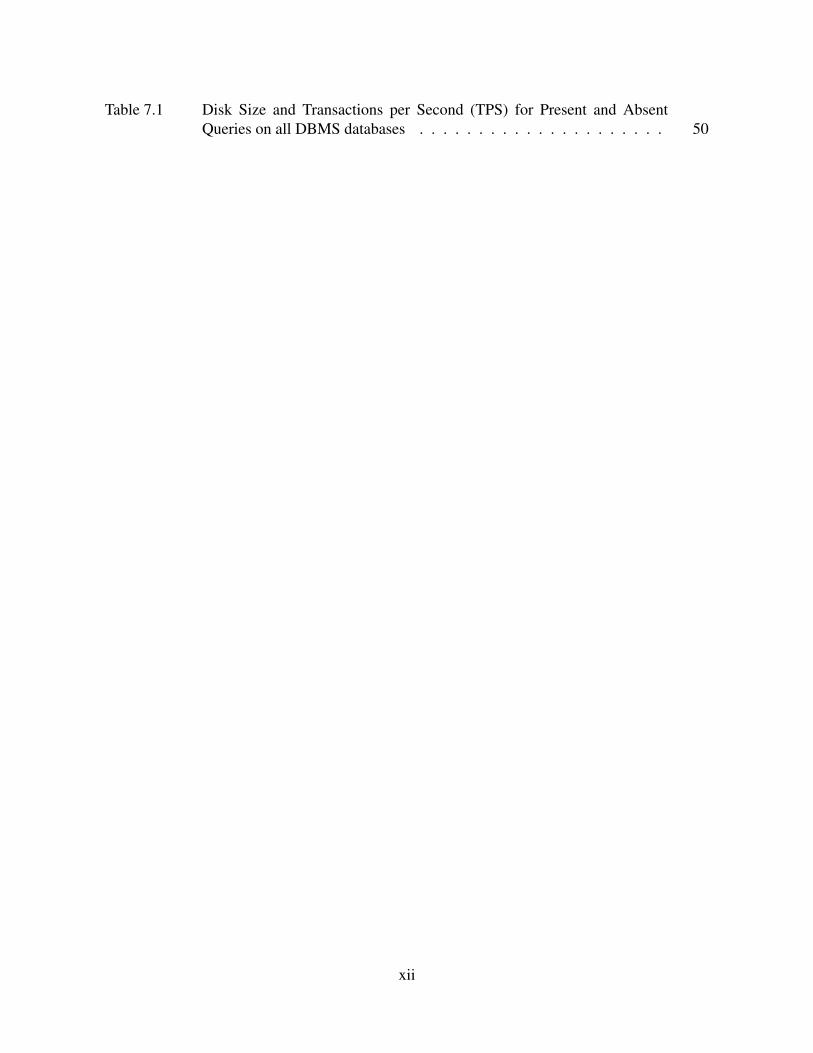
Table 7.1 Disk Size and Transactions per Second (TPS) for Present and AbsentQueries on all DBMS databases . . . . . . . . . . . . . . . . . . . . . 50

xii

List of Acronyms and Abbreviations

ASCII American Standard Code for Information Interchange

b bit

B Byte

BF Bloom Filter

BtrFS B-tree File System

CRC32 Cyclic Redundancy Check (32 bits)

CRC64 Cyclic Redundancy Check (64 bits)

DBMS Database Management System

EXT3 Third Extended File System

EXT4 Fourth Extended File System

FBHMA File Based Hash Map Analysis

FAT File Allocation Table

GB Gigabyte (109 bytes)

GiB Gibibyte (230 bytes)

Govdocs1 Million Government Document corpus

html HTML file extension

HTML HyperTExt Markup Language file format

jpg JPEG file extension

JPEG Joint Photographic Experts Group file format

K Thousand (103)

KB Kilobyte (103 bytes)

KiB Kibibyte (210 bytes)

M Million (106)

MB Megabyte (106 bytes)

xiii

MD5 MD5 message digest algorithm

MiB Mebibyte (220 bytes)

OCMalware Offensive Computing Malware corpus

OS Operating System

NOOP No Operation assembly instruction

NoSQL “Not only SQL” model for non-relational database management

NSRL National Software Reference Library

NSRL RDS NSRL Reference Data Set

NTFS New Technology File System

pdf PDF file extension

PDF Adobe Portable Document Format

PE Portable Executable file format

RAM Random access memory

RPC Remote procedure call

SHA-1 Secure Hash Algorithm, version 1

SHA-3 Secure Hash Algorithm, version 3

SQL Structured Query Language for relational database management

TB Terabyte (1012 bytes)

TiB Tebibyte (240 bytes)

TPS Transactions per Second

txt TXT file extension

TXT ASCII text file

UPX The Ultimate Packer for eXecutables

xiv

Acknowledgements

I would like to thank Dr. Simson Garfinkel for his outstanding mentorship. I am grateful for hisguidance throughout the thesis process, the opportunities he made available to share my workwith the community and his strong example of leadership and technical expertise.

I would also like to thank Mr. Neal Ziring for being my second reader and providing carefulinsight and feedback on the thesis. Mr. Ziring has been a long time unofficial mentor of mineand I appreciate his willingness to invest his time and impart invaluable guidance and advice.

I would like to thank Dr. Joel Young for his guidance and willingness to assist me in variousparts of my thesis. His instruction in experiment design and database performance was criticalto obtaining sound and accurate results.

Thank you to all of the professors who provided instruction and guidance during my time atNPS. My experience was greatly enriched through our interactions.

Finally, I would like to thank my mother, Berdia, and fiance, Dewey. I thank God for such astrong support system that keeps me focused and encouraged. I could not do it without youall.

xv


xvi

CHAPTER 1:Introduction

Quickly identifying content of interest on digital media is critical to the forensic investigationprocess. Given a large disk or set of disks, an examiner requires an efficient triage processto determine if known content is present. Today, examiners identify content by comparingfiles stored on the target media to a database of known file hashes collected from previousinvestigations. Traditional forensic tools identify stored files by analyzing the file system orcarving files based on headers and footers [1–4].

Analyzing the file system to identify content has several shortcomings. Relevant content maybe stored in areas that are not directly parsed by the file system, such as unallocated or slackspace. Portions of files or the file system may be unreadable due to partial overwriting or mediafailure. The current methods are not robust to new or unknown data types, file formats or filesystems. Finally, the entire file system must be read to find files of interest and the searchprocess is difficult to parallelize due to the file system tree structure [5].

Although file carving addresses some of these issues by parsing the raw bytes on the disk,carving itself has several shortcomings. For example, file carving based on headers and footersis not effective at identifying content from overwritten or partially destroyed files, or contentthat is fragmented into multiple locations on the media. File carving is also prone to falsepositives.

1.1 How distinct sector identification worksWe propose a forensic method that uses sector hashing to quickly identify content of interest.Using this method we search for content in disk sectors, fixed-sized chunks of physical diskthat are the smallest unit to which data can be written. Current file systems such as FAT, NTFS,Ext3 and Ext4 and next generation file systems such as ZFS and the B-tree File System (BtrFS)write files on sector boundaries. The standard sector size is 512 B, although most modern disksare moving to 4 KiB for format efficiency and more robust error correction [6]. For example,when a 60 KB JPEG file is stored, the first 512 B are written to one sector, the second 512 Bare written to the next sector and so on. Because most files are sector aligned, we can search forcontent by comparing the hash of each 512 B or 4 KiB disk sector on the target media to a hashdatabase of fixed-sized file fragments of the same size, which we call file blocks.

1

Full Media Analysis

2 TB Drive4 Billion

512 B Sectors File 3 File 3

A J K D L

File 1

512 B Sector

A B C D E

File 2

F G H A I

Incomplete Files

Intact Files

Block

A

B

C

D

E

F

G

H

File Block Occurs In

File 1, File 2, File 3

File 1

File 1

File 1, File 3, File 99

File 1

File 2

File 2

File 2

1 BillionRows

File Block Hash Database

1 TB Drive2 Billion

512 B Sectors

Media Sampling

B

A

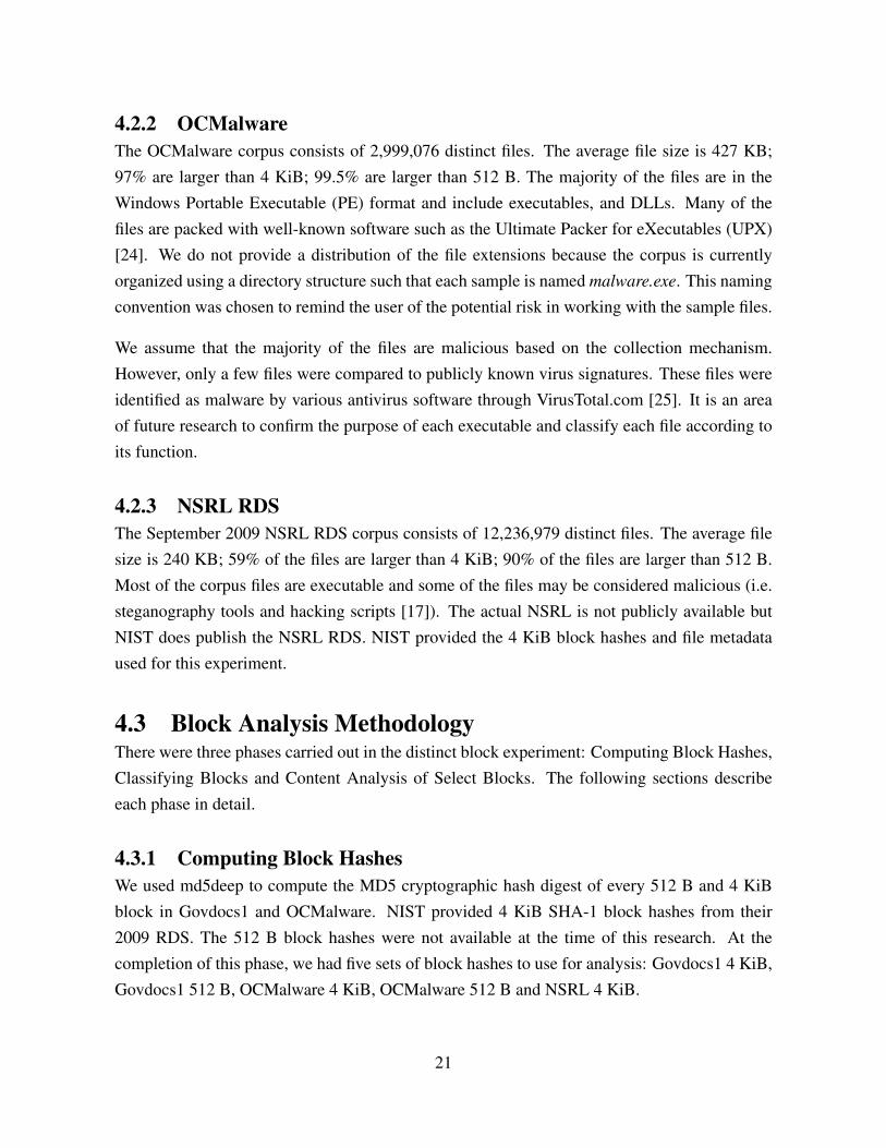
Figure 1.1: Because files are stored on sector boundaries, we can search disk sectors for file blocks, or fixed-sizedchunks of data equal in size to the disk sectors. We create a file block hash database that contains block hashes forevery file that we have ever seen during an investigation. A database with 1 billion 512 B block hashes can reference476 GB of content. Sector hashing depends on the existence of distinct file blocks, or blocks that only occur as acopy in the original file. With full media analysis, all 4 billion sectors from the 2 TB drive are compared to the fileblock hash database. With media sampling, only 1 million of the 2 billion sectors from the 1 TB drive are compared toidentify a 4 MB file that has all distinct blocks with 98.17% accuracy. If block B is seen on a disk sector, then thereis a good chance that File 1 also exists on the disk. Block B only occurs in one file in our large corpus of known filesand is effectively distinct. If Block A is seen on a disk sector, then we are not sure if any of the files exist. Block A isnon-distinct. Sector hashing can quickly identify fully intact and incomplete files that contain distinct blocks.

This example demonstrates the use of sector hashing to identify the presence of three files (1,2 & 3) on the subject media. The block hash database contains all of the blocks from a corpusof every file that has ever been seen during an investigation. The database is a key-value storewhere the key is a hash of a file block and the value is a list of every file in which the blockoccurs.

Figure 1.1 is a graphical representation of a 2 TB disk that has four billion 512-byte sectors. Itcontains three previously seen files; File 1, File 2 and File 3. File 1 and File 2 are both 60 KBJPEG images that have 120 512-byte blocks, matching the sector size. The files are intact,which means that every file block is currently stored in a disk sector. As shown in Figure 1.1,

2

File 1 contains blocks A - E and File 2 contains blocks A and F - I.

File 3 is a 4 MB high-resolution JPEG image that has 8,192 blocks. This file is incomplete be-cause some of the sectors that previously stored its blocks have been overwritten. The remainingblocks have not been overwritten and are stored in the disk sectors. This scenario occurs after afile is deleted and the containing sectors are made available for new files. File 3 contains blocksA, D and J - L.

1.1.1 Sector hashing and full media analysis for residual data identifica-tion

Using sector hashing in full media analysis, we compare every sector of the 2 TB disk to theblock hash database. When the sector that contains block B is identified, we know that File 1may be present on the disk because block B only occurs in File 1 of all the files in our corpus.We do not know if File 1 is definitely present because block B could occur in a different filethat is not included in our corpus–knowing that block B is present is not sufficient to prove thatFile 1 is also present. When the sector that contains block A is identified, we have even lessconfidence that File 1, File 2 or File 3 are present. Since Block A occurs in multiple files in ourcorpus, we believe the block likely occurs in other files that are not in our corpus–knowing thatblock A is present does not prove that any of the files from our corpus are present.

Sector hashing for file identification depends on the existence of distinct blocks, or blocks thatonly occur on media as a copy of the original file for all files. We cannot prove that a block isuniversally distinct. However, we can treat blocks that only occur once in a large file corpus,such as block B in our example, as if it were universally distinct. Doing so allows us to quicklyfind evidence that a file is present on disk. Deeper file-level analysis is used to confirm the file’spresence.

After analyzing all of the sectors from our target disk we learn that all of the blocks from File 1and File 2 and some of the blocks from File 3 are stored on the disk. If the majority of File 1’sblocks do not occur in any other corpus file, then the results provide strong evidence that File 1is currently present on the disk. The same is true for File 2. If File 3’s block are also notrepeated elsewhere, then the results provide strong evidence that File 3 was once present on thedisk.

3

1.1.2 Sector hashing and random sampling for triageUsing sector hashing for media sampling also allows for a faster triage process. Instead ofsearching all of the disk sectors, we can search a sample set of randomly chosen sectors todetermine with high probability that a file is present as illustrated in Figure 1.1. The samplesize must be large enough to ensure that we will almost certainly select a sector that contains atleast one of the blocks in the file if it is present. We can determine an appropriate sample sizeusing the well known “urn” problem, a statistical model that describes the probability of pullingsome number of red beans out of an urn that contains a mix of red and black beans randomlydistributed [7].

The red beans are the sectors that contain the distinct blocks of the content we are trying toidentify. The black beans are sectors that do not contain the distinct blocks, all remainingsectors. The total number of beans is the number of sectors on the target media. If we are tryingto identify a 4 MB JPEG of all distinct blocks on a 1 TB drive, there are 8,000 red beans (C),and 2 billion beans in total (N). If we randomly select 1 million (n) beans we have a 98.17%chance of selecting a red bean at least once, or detecting the 4 MB file.

Equation 1.1 calculates the probability of not finding even a single red bean in n draws andsubtracts that from one to get p, the probability that at least one red bean is found in n draws:

p = 1−n

∏i=1

((N− (i−1))−C)

(N− (i−1))(1.1)

Using sector hashing with random sampling provides a quick triage method to determine if a fileof interest is likely present on a target media. The method is file system and file type agnostic;as long as we can read the disk sectors and have a copy of the file in our block hash database, wecan use sector hashing to find evidence of the file on disk. Sector hashing can also find evidenceof a file that was once present but has been partially overwritten and is not fully recoverable.

1.2 Design IssuesThere are several design issues in implementing media analysis with sector hashing. The first ischoosing an appropriate block size for the hash database. We considered both 512 B and 4 KiB,the standard sector sizes for current drives. Using 512 B blocks allows for more granularity inthe search but requires that we store eight times as many hashes—there are eight 512 B blocksin every 4 KiB block. As discussed in Chapter 7, the size of the block hash database has a

4

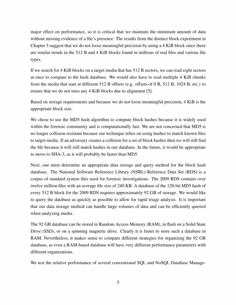
major effect on performance, so it is critical that we maintain the minimum amount of datawithout missing evidence of a file’s presence. The results from the distinct block experiment inChapter 5 suggest that we do not loose meaningful precision by using a 4 KiB block since thereare similar trends in the 512 B and 4 KiB blocks found in millions of real files and various filetypes.

If we search for 4 KiB blocks on a target media that has 512 B sectors, we can read eight sectorsat once to compare to the hash database. We would also have to read multiple 4 KiB chunksfrom the media that start at different 512 B offsets (e.g. offsets of 0 B, 512 B, 1024 B, etc.) toensure that we do not miss any 4 KiB blocks due to alignment [5].

Based on storage requirements and because we do not loose meaningful precision, 4 KiB is theappropriate block size.

We chose to use the MD5 hash algorithm to compute block hashes because it is widely usedwithin the forensic community and is computationally fast. We are not concerned that MD5 isno longer collision resistant because our technique relies on using hashes to match known filesto target media. If an adversary creates a collision for a set of block hashes then we will still findthe file because it will still match hashes in our database. In the future, it would be appropriateto move to SHA-3, as it will probably be faster than MD5.

Next, one must determine an appropriate data storage and query method for the block hashdatabase. The National Software Reference Library (NSRL) Reference Data Set (RDS) is acorpus of standard system files used for forensic investigations. The 2009 RDS contains overtwelve million files with an average file size of 240 KB. A database of the 128-bit MD5 hash ofevery 512 B block for the 2009 RDS requires approximately 92 GB of storage. We would liketo query the database as quickly as possible to allow for rapid triage analysis. It is importantthat our data storage method can handle large volumes of data and can be efficiently queriedwhen analyzing media.

The 92 GB database can be stored in Random Access Memory (RAM), in flash on a Solid StateDrive (SSD), or on a spinning magnetic drive. Clearly it is faster to store such a database inRAM. Nevertheless, it makes sense to compare different strategies for organizing the 92 GBdatabase, as even a RAM-based database will have very different performance parameters withdifferent organizations.

We test the relative performance of several conventional SQL and NoSQL Database Manage-

5

ment Systems (DBMS) in managing a database of one billion hashes. With a 4 KiB block size,one billion hashes allows us to index 4 TB of content. Our results show that a custom storagesolution is required to support the hash lookup speeds that our application requires.

A third issue is determining the occurrences of distinct blocks in our file corpora. We analyzethree multi-million file corpora that contain real documents, system files, and legitimate and ma-licious software. To our knowledge, there are no previous studies analyzing the co-occurrenceof blocks across such a large number of files and file types. By using these corpora we can beginto make general conclusions about the true frequency of distinct blocks. Our findings suggestthat most files are made up of distinct blocks that identify a single specific file.

We are also interested in determining rules to quickly eliminate disk sectors that store file blocksthat are common among many documents or file types. These sectors can be ignored early in theanalysis process. Omitting likely non-distinct sectors will improve performance by minimizingthe number of disk sectors that are compared to the file block hash database.

The fourth issue is determining the appropriate tool architecture for use in the field. There arenumerous restrictions that we consider for deployed operations including limited storage spaceand computational power.

1.3 Distinct BlocksIdentifying files with sector hashes relies on the presence of distinct file blocks. A distinct

block is one that does not exist more than once in the universe except as a block in a copy of theoriginal file. Using distinct blocks as a forensic tool leverages two hypotheses [5]:

1. If a block of data from a file is distinct, then a copy of that block found on a data storagedevice is evidence that the file is or was once present.

2. If the blocks of that file are shown to be distinct with respect to a large and representativecorpus, then those blocks can be treated as if they are universally distinct.

The first hypothesis is true by the definition of distinct blocks. If the block only exists as a blockin a specific file, then if the block is found on a piece of target media then the file must exist orhave previously existed.

The second hypothesis deals with the method of determining if a file block is distinct. It is im-possible to prove that a block is universally distinct because doing so would require comparing

6

the block to every block. However, we can identify blocks that only appear once in millions offiles and treat them as if they were universally distinct in the context of finding possible evidencethat a file once existed on a piece of media. Making such a finding requires that we tabulateall the blocks in a sufficiently large corpus that contain the same file types as from which thepotentially distinct block came.

We performed this exercise with three large file corpora that each contain millions of files ofvarious file types including documents, operating system files and legitimate and malicioussoftware. We find that the overwhelming majority of the file blocks were distinct with respectto each corpus (and between corpora as well) and could therefore be used to identify a singlespecific file.

Ideally all files would consist of mostly distinct blocks, or blocks that only occur in one specificfile. Finding one distinct block from a file on a target disk is not as convincing as findingmultiple distinct blocks from the same file on disk. Furthermore, if we find many distinctblocks from a specific file and if the blocks are stored contiguously, we have higher confidencethat the file exists or previously existed.

1.4 Usage ModelsOur primary usage model is a single system field deployment on a consumer laptop or desktop.In this model, the block hash database is stored locally or on a piece of removable media. Thecurrent storage capacity of commodity drives and external media is as large as a few terabytes insize. This is sufficient to store the block hashes of as many as one billion files. To store the MD5block hashes of 1 billion files with an average size of 512 KB and a file block size of 4 KiBrequires 2 TB of storage. This size will fit into the largest storage capacity of a commoditysystem or external storage device available for purchase today.

The limitation of using a single system model is the available memory. The current maximummemory available for a consumer laptop system is 16 GiB. As discussed in Chapter 7, theconventional DBMSs perform best when the database fits into memory. For the conventionalDBMSs studied, 16 GiB can contain the block hash database for 100 million block hashes–the1 billion hash database has an average size of 112 GB. For a block size of 4 KiB, 100 millionblock hashes represents 400 GB of content. This amount of content can support a few hundredmillion files with an average file size of 512 KB.

Another limitation is that only one examiner can use the system at a time, as the database is

7

only locally available. However, this model is typical for field deployed systems and we focusour analysis on the single system model for this thesis.

A second usage model is the client/server model. In this model, the block hash database isstored on a remote server and accessed by many clients simultaneously. Similar to the singlesystem model, the server can store the database locally or use external media. Servers typicallyhave significantly more local storage space than a laptop or desktop. Servers also have morememory, typically a couple hundred gigabytes which easily supports the 1 billion hash databasestored by all the conventional DBMSs used in this thesis.

The client reads the target media and sends the sector hashes to the database for comparison.For this model, we must consider the network throughput and latency. Throughput will limitthe maximum number of hashes that can be searched per unit time. Latency is an issue withsimplistic designs that do not rely on asynchronous Remote Procedure Calls (RPC).

The final usage model is a distributed database model. In this model, the hash database is splitbetween multiple database servers. Because hash values are evenly distributed it is trivial toparallelize the database using prefix routing [8]. A cluster with 1,000 servers that each managea database of 1 billion 4 KiB blocks can address four petabytes of known content. The benefitof the distributed database model is that it maintains the performance of a smaller databasebecause each server only manages 1 billion hashes. Similar to the client/server model, theeffects of network throughput is a factor but the impacts of latency are minimal if the lookupsare batched and pipelined.

1.5 Chapter OutlineThe following chapters discuss several of the design issues for implementing sector hashes forforensic triage analysis. Chapter 2 discusses prior work using content hashing to identify files.Chapter 3 provides a classification framework to discuss file block types. Chapters 4 and 5 dis-cuss an experiment to determine the number of distinct blocks in three large file corpora of over15 million files including user-generated documents, system files, legitimate and malicious soft-ware. Chapters 6 and 7 discuss an experiment to determine if conventional databases can meetthe performance requirements of our file block hash database. Chapter 8 concludes, discussesthe limitations of sector hashing and presents future work.

The major contributions of this thesis are: (1) the empirical evidence of distinct blocks in mil-lions of files of various file types that can be used to identify a specific file, and (2) relative

8

performance analysis of conventional DBMSs in storing 1 billion hashes.

9


10

CHAPTER 2:Prior Work

This review spans two major forensic research areas; file identification and large hash databases.

2.1 File IdentificationTraditionally, files are identified in forensic processing using file system metadata and carving.File metadata consists of information such as file name, creation time, size and the location ofthe file on disk. The metadata is stored in file system data structures that must be intact anddecodable. This is the most straight-forward method to identify a file but metadata is triviallymodified to hide the presence of a file without corrupting the contents.

File carving is the practice of searching an input for files or other kinds of objects based oncontent, rather than on metadata [9]. It is a powerful tool for recovering files and fragments offiles when metadata is corrupt or missing either due to deleted files or damaged media. Most filecarvers operate by looking for file headers and/or footers, distinct tags at the beginning and endof the file, and carving out the blocks between these two boundaries. More complex methodsare needed to handle fragmented files. Various file carving methods are listed in Table 2.1.

Hash-based carving is the same idea as the distinct block identification presented in this thesis.frag_find is a forensic tool that performs hash-based carving [10]. The tool greedily searches thedisk image for the longest run of sectors that match a contiguous series of file blocks. frag_find

stores the entire sector hash database in RAM using an Standard Template Library (STL) map(a red-black tree). Its operation relies on the existence of distinct blocks and distinct blocksequences. Although frag_find was published several years ago, there was no follow up workuntil this thesis and there has never before been a study of the prevalence of distinct blocks.

Dandass et al. present a case study where they analyzed hashes for over 528 million sectorsextracted from over 433,000 files. They computed SHA-1, MD5, CRC32 and CRC64 hashes foreach sector and compared the algorithms according to the number of false-positive indicationsand the storage capacity for the entire hash collection. The authors found no collisions witheither the SHA-1 or MD5 algorithms but found that CRC64 had low collision rates and requiredonly half the storage space. Dandass et al. conclude that CRC64 could be used as a filteringalgorithm to extract sectors that do not match sectors from a collection of known illicit files [11].

11

Carving Method DescriptionBlock-based carving Analyzes each block of the input to determine if the block

is part of a file.Statistical carving Analyzes certain characteristics or statistics of the input,

such as entropy, to determine which parts make up the file.File structure carving Carves files based on the internal structure of file types.Semantic carving Analyze the meaning of the input, such as linguistic analysis.Carving with validation Uses a file type validator to confirm carved files.Fragment recovery carving Reassembles two or more fragments to form the original file or

object.Hash-based carving Hashes portions of the input and searches for matches to hashes

of known files.

Table 2.1: Garfinkel and Metz propose the listed methods as a file carving taxonomy [9]. File carving tools that usefile meta data or the file’s internal structure are usually only effective at identifying fully intact and contiguously storedfiles. Tools based on the other methods, block-based, statistical, semantic, validation, fragment and hash-based, canidentify fragments of a file by searching for exact matches or characteristics that are prevalent throughout a file.

However, follow up work by Garfinkel questioned this work as modern MD5 implementationsare actually faster than CRC64 implementations and MD5 can take the same amount of storageas CRC64 if only half of the hash is retained.

The EnCase File Block Hash Map Analysis (FBHMA) EnScript is another sector hashing toolthat searches for file blocks in disk sectors [12]. The script creates a database of target fileblock hashes from a master list and searches selected disk sectors for the file blocks. FBHMAalso carves files using sector hashing, including files that have been partially overwritten ordamaged. This tool was primarily designed to search file slack space, unused disk areas andunallocated clusters and not entire disks. It is not optimized for full media analysis and cannotperform sampling.

The md5deep tool suite also supports sector hashing [13]. md5deep is a set of tools to computecryptographic message digests, including piecewise hashes, on an arbitrary number of files. Thetool supports searching for file block hashes in media sectors. We used md5deep extensively inthis thesis to compute the block hashes of our file corpora. Like the other sector hashing tools,md5deep is not optimized to support a large database of hashes and cannot perform sampling.

Wells et al. used block hash filtering to extract the most interesting data from a mobile phonefor forensic investigations [14]. They divide media into small fixed-sized overlapping blocksand use block hashes for deduplication. The media blocks that match a library of known mediablock hashes computed from other phones are excluded under the assumption that matchingblocks do not contain information of interest to investigators. According to their findings, theirmethod reduces the amount of acquired data from collected phones by 69%, on average, without

12

removing usable information.

2.2 Large Hash DatabasesA critical issue with sector hashing is the performance requirements for a large and fast databaseof file block hashes. For the single system usage model, the database must be small enough tofit on a consumer laptop or external storage device and the query rate must be fast enough toallow for rapid triage, identifying potential files of interest as quickly as the media can be read.There has been several research initiatives to determine the best method to store and query largecollections of sector hashes.

Collange et al. present a file fragment data carving method using Graphical Processing Units(GPUs). They compute hashes for every 512 B disk sector and compare the hashes to 512 Bblocks from known image files. If there is a match, then the disk is flagged to signify that a file ofinterest potentially existed on the disk and that it requires deeper analysis. Taking advantage ofthe multiple cores in a GPU, they implement a parallel pattern matching engine that can processevery 64 B fragment aligned on 32-bit boundaries in disks at a sustained rate of approximately500 MB/s [15].

Farrell et al. evaluate the use of Bloom filters (BFs) to distribute the National Software Ref-erence Library’s (NSRL) Reference Data Set (RDS) [16]. The NSRL RDS is a collection ofdigital signatures of known, traceable software applications [17]. The evaluation was conductedwith version 2.19 of the NSRL RDS that contains approximately 13 million SHA-1 hashes.Bloom filters were thought to be an attractive way for handling large hash sets because the datastructure is space efficient. Farrell et al. could only obtain 17 K to 85 K RDS hash lookupsper second using SleuthKit’s hfind command and only 4 K lookups per second using a MySQLInnoDB database. Using a new BF implementation on the same hardware, query rates between98 K and 2.2 million lookups per second were achieved. However, using BFs makes it dramati-cally easier for an attacker to construct a hash collision in comparison with a collision-resistantfunction such as SHA-1. The authors comment that an attacker could leverage the vulnerabilityto hide illicit data when BFs are used to eliminate “known goods“ [16].

13


14

CHAPTER 3:Taxonomy

This chapter presents a taxonomy for classifying blocks that we will use in the distinct blockexperiments.

3.1 Block ClassificationThe principal classification of a block is based on the number of times the block occurs in acorpus. Blocks that occur exactly once in the corpus are called singletons; blocks that occurexactly twice are called pairs; blocks that occur three or more times are called common. Wecreated the three categories based on initial observations and then formed our hypothesis of theroot causes for the frequency of occurrence to fit the observations.

Singleton blocks are those blocks that were found just once in the corpus. Pair blocks are thosethat were found twice. We hypothesize that pair blocks occur in files that are related, eitherbecause one file is embedded or contained in the other file or because one file is a modifiedversion of the other file. Common blocks occur more frequently and we expect them to existdue to a commonality between all files or file types. For example, the block of all NULs (0x00)is a common block that is used to pad data in a file. In fact, the block of NULs is the mostcommon block in our corpus.

The secondary classification of a block is based on the characteristics of its content. For ouranalysis, we classify blocks based on the byte entropy and the length of any repeating n-grams.We use Shannon entropy to measure the predictability of the byte values in each block [18]. Anentropy score of 0 means that the block has 0 bits of entropy per byte and has a single byte valuerepeated throughout the block, for example the block of all NULs (0x00). An entropy score of 8means that the block has 8 bits of entropy per byte and any byte value is equally likely to appearin the block, for example an encrypted block that resembles random data.

We also classify blocks based on the existence and length of the shortest repeating n-gram. Ann-gram is a chunk of n-bytes. If a block consists of a byte pattern, or repeating n-gram, thatrepeats throughout the block, we call it a repeating n-gram block. The length of the n-gramcan be as small as one byte and as large as half of the block size. For 512 B blocks, the largestrepeating n-gram is 256 bytes and for 4 KiB blocks, the largest repeating n-gram is 2,048 bytes.

15

Classification DefinitionPrincipal ClassificationSingleton Appear only once in a corpusPairs Appear exactly twice in a corpusCommon Appear three or more times in a corpusSecondary ClassificationEntropy Predictability of byte values in the block (0-8)Repeating n-gram Block Contains a repeating n-gramN-gram Size The size n of the repeating n-gram (0-half of block size)

Table 3.1: A list of the principal and secondary classification of file blocks in the corpora.

It is important to note that the last instance of the repeating n-gram may not fully repeat beforethe end of the block. For example, the string abcabcab consists of a repeating 3-gram ‘abc’ thatis repeated twice and starts to repeat in the end of the string. It is also important to note that wedo not look for blocks that consist of repeated byte sequences separated by variable data. Forexample, the string abracadabra obviously consists of a repeated 4-gram ‘abra’ but the patternis interrupted with other variable data so the string is not considered a repeating n-gram.

We found many examples of common blocks with various entropy values and repeating n-grams. In general, we found that most blocks with low entropy or repeating n-grams werecommon, making these tests a useful prefilter.

Table 3.1 summarizes the block classifications used for our research.

3.2 Future Block ClassificationAn additional classification category that was considered but not used is based on printableASCII strings found in a file block. Strings-based file identification is commonly used in foren-sics and malware detection and is also useful for our method [19,20]. All of the documents fromthe million government document corpus [21] (Govdocs1) were downloaded from governmentwebsites and most of the documents were in a human readable format (i.e. PDF, HTML, DOC,TXT). As a result, many of the blocks contain printable ASCII strings.

There are several expected types of string-based n-grams such as a string of all spaces, govern-ment related terms, any word in the English language and textual representation of numbers. Ifthe strings are distinct we want to search for other blocks that have the same strings to identifyother copies of the file. On the other hand, if the strings are common and repeated in many filewe will not use it to identify a specific file.

Due to the time constraints of our research, we did not pursue string-based block classification

16

Classification DefinitionAll spaces Consists of a string of space characters (0x20)Government related terms Consists of government-related wordsTextual Representation of #s Consists of textual representation of numbers

Table 3.2: A list of potential string-based secondary block classification categories.

but believe that it should be studied in future research in distinct block identification.

Table 3.2 summarizes the string-based classifications.

17


18

CHAPTER 4:Distinct Block Experiment

The objective of the distinct block experiment was to determine the occurrences of distinctblocks in a large collection of files. We hoped that a significant number of file blocks wouldbe distinct in our corpus justifying the use of distinct blocks for identifying the presence of asingle file. To this end we examined millions of real files and enumerated the number of distinctblocks.

To our knowledge, there are no previous studies analyzing the co-occurrence of blocks acrosssuch a large number of files and variety of file types. By using these corpora we can begin tomake general conclusions about the true frequency of distinct blocks.

4.1 ResourcesWe used three existing file corpora to perform the experiments. Together, these corpora repre-sent over 15 million files. The million government document corpus (Govdocs1) is a collectionof nearly one million freely-redistributable files that were obtained by downloading contentfrom web servers in the .gov domain [21]. The Offensive Computing Malware corpus (OCMal-ware) is a collection of approximately 3 million malware samples that were acquired from var-ious collection and trading networks world wide [22]. The National Institute of Standards andTechnology (NIST) National Software Reference Library (NSRL) Reference Data Set (RDS)is a collection of known, traceable software applications [17]. All three corpora consist of realdata, and Govdocs1 and NSRL RDS contain additional provenance such as the original filename and creation date.

We used md5deep and Digital Forensics XML (DFXML) to compute and process the MD5 hashof each block in the file collection. md5deep is a set of cross-platform tools to compute messagedigests for an arbitrary number of files [13]. The tool can also compute piecewise hashes wherefiles are broken into fixed sized blocks and hashed. md5deep can be configured to output thehashes in DFXML format. DFXML is an initial XML schema that provides common tags toallow for easy interoperability between different forensic tools [23].

We wrote tools to analyze the block hashes computed by md5deep using using Garfinkel’s C++DFXML processing libraries [23] as the Python implementation was too slow and required too

19

Count Extension Count Extension Count Extension Count Extension231,512 pdf 10,098 log 254 txt 14 wp190,446 html 7,976 UNK 213 pptx 8 sys108,943 jpg 5,422 eps 191 tmp 7 dll

83,080 text 4,103 png 163 docx 5 exported79,278 doc 3,539 swf 101 ttf 5 exe64,974 xls 1,565 pps 92 js 3 tif49,148 ppt 991 kml 75 bmp 2 chp41,237 xml 943 kmz 71 pub 1 squeak34,739 gif 639 hlp 49 xbm 1 pst21,737 ps 604 sql 44 xlsx 1 data17,991 csv 474 dwf 34 jar13,627 gz 315 java 26 zip

Table 4.1: The Govdocs1 corpus contains mostly human readable documents and images. Adobe PDF, MicrosoftOffice, HTML, log files and graphical image files make up the majority of the corpus. Through our block level analysis,we find that most files have correct extensions that match the file type, but some files do not. For example, the fileswith extension txt are all HTML documents.

much memory.

4.2 File CharacteristicsEach of the three file corpora represent different types of files. OCMwalware and the NSRLRDS consist of mostly executable content and Govdocs1 consists of mostly non-executabledocuments. Based on the collection methodology and purpose of each corpus, OCMalware hasmostly malicious content while Govdocs1 and NSRL RDS have mostly non-malicious files. Itis useful that we analyzed corpora that have different types of files to determine if the exis-tence of distinct blocks is a general characteristic. The following subsections provide additionalinformation about the files in each corpus.

4.2.1 Govdocs1The Govodcs1 corpus consists of 974,777 distinct files. The majority of the files are AdobePDF, Microsoft Office, graphical image files and ASCII text. The average file size is 506 KB;93% of files are larger than 4 KiB; 99% of files are larger than 512 B.

Table 4.1 summarizes the file types in the Govdocs1 corpus according to the file extension onthe originally downloaded file. Although we do not confirm the file type for all files, we verifiedmany of the file extensions during block content analysis discussed in Section 5.2 with the Unixfile command and with visual inspection. There are instances of file extensions that do notmatch the file type, such as the files with the txt file extension that are HTML documents.

20

4.2.2 OCMalwareThe OCMalware corpus consists of 2,999,076 distinct files. The average file size is 427 KB;97% are larger than 4 KiB; 99.5% are larger than 512 B. The majority of the files are in theWindows Portable Executable (PE) format and include executables, and DLLs. Many of thefiles are packed with well-known software such as the Ultimate Packer for eXecutables (UPX)[24]. We do not provide a distribution of the file extensions because the corpus is currentlyorganized using a directory structure such that each sample is named malware.exe. This namingconvention was chosen to remind the user of the potential risk in working with the sample files.

We assume that the majority of the files are malicious based on the collection mechanism.However, only a few files were compared to publicly known virus signatures. These files wereidentified as malware by various antivirus software through VirusTotal.com [25]. It is an areaof future research to confirm the purpose of each executable and classify each file according toits function.

4.2.3 NSRL RDSThe September 2009 NSRL RDS corpus consists of 12,236,979 distinct files. The average filesize is 240 KB; 59% of the files are larger than 4 KiB; 90% of the files are larger than 512 B.Most of the corpus files are executable and some of the files may be considered malicious (i.e.steganography tools and hacking scripts [17]). The actual NSRL is not publicly available butNIST does publish the NSRL RDS. NIST provided the 4 KiB block hashes and file metadataused for this experiment.

4.3 Block Analysis MethodologyThere were three phases carried out in the distinct block experiment: Computing Block Hashes,Classifying Blocks and Content Analysis of Select Blocks. The following sections describeeach phase in detail.

4.3.1 Computing Block HashesWe used md5deep to compute the MD5 cryptographic hash digest of every 512 B and 4 KiBblock in Govdocs1 and OCMalware. NIST provided 4 KiB SHA-1 block hashes from their2009 RDS. The 512 B block hashes were not available at the time of this research. At thecompletion of this phase, we had five sets of block hashes to use for analysis: Govdocs1 4 KiB,Govdocs1 512 B, OCMalware 4 KiB, OCMalware 512 B and NSRL 4 KiB.

21

4.3.2 Classifying BlocksWe created a C++ program sector_stats to analyze the hashes generated by md5deep. Theprogram counts the number of singleton, pair and common blocks as defined in Chapter 3 foreach of the five hash sets. We only include full blocks and ignored files and end blocks thatwere smaller than 512 B or 4 KiB in size.

Our program also checks for duplicate files using the MD5 file hash provided in the md5deepoutput and ignores any files that had been previously processed.

4.3.3 Content Analysis of Most Common and Random BlocksWe analyzed the top 50 most common blocks and 50 other randomly selected pair and commonblocks in Govdocs1 and OCMalware to try to understand the reason that the blocks occurred inmultiple files. For each block, we determine how many unique files and file types (as reportedby the file command) the block occurred in as well as the entropy and pattern size of the blockcontent. We also extract a sample of the block from a file in the corpus using dd and examinethe contents with hexdump. When appropriate, we also viewed a sample of files that containedthe block with emacs or the corresponding file viewer.

This analysis provided insight into the root cause of non-distinct blocks and identified severalfile-type specific block patterns that could be used to identify types of files.

Chapter 5 discusses the results of these experiments.

We did not perform this analysis with the NSRL blocks since we did not have a copy of theoriginal files.

22

CHAPTER 5:Distinct Block Experiment Results

This chapter discusses the results of the distinct block experiment with the million governmentdocument corpus (Govdocs1), the Offensive Computing Malware corpus (OCMalware) and theNational Institute of Standards and Technology (NIST) National Software Reference Library(NSRL) Reference Data Set (RDS) (NSRL2009).

5.1 Block ClassificationAs demonstrated in Table 5.1, the vast majority of blocks in each corpus are singletons andcorrespond to a single, specific file. This is not surprising. High entropy data approximates arandom function. A truly random 512 B block contains 4,096 bits of entropy. There are thus24,096 ≈ 101,200 possible different blocks and they are all equally probable. It is therefore in-conceivable that two randomly generated blocks would have the same content. The randomnessof user-generated content is less than 8 bits per byte, of course, but even for content that has anentropy of 2 bits per byte there are still 1,024 bits of entropy in a 512B block, making it onceagain very unlikely that a block will be repeated by chance in two distinct files [7].

Table 5.2 shows that all kinds of user-generated content from Govdocs1, including word pro-cessing files and still photographs contains blocks that are only seen in one file in a large corpusof files. According to the distinct block hypothesis, these singletons can be treated as univer-sally distinct blocks and used to find evidence that a particular file once existed on investigationmedia.

Govdocs1 OCMalware NSRL2009Total Unique Files 974,741 2,998,898 12,236,979Average File Size 506 KB 427 KB 240 KBBlock Size: 512 BSingletons 911.4M (98.93%) 1,063.1M (88.69%) n/a n/aPairs 7.1M (.77%) 75.5M (6.30%) n/a n/aCommon 2.7M (.29%) 60.0M (5.01%) n/a n/aBlock Size: 4 KiBSingletons 117.2M (99.46%) 143.8M (89.51%) 567.0M (96.00%)Pairs 0.5M (.44%) 9.3M (5.79%) 16.4M (2.79%)Common 0.1M (.11%) 7.6M (4.71%) 7.1M (1.21%)

Table 5.1: Occurrences of singleton, pair and common blocks in the Govdocs1, OCMalware and NSRL2009 corpora.

23

Extension File 4 KiB Block % Singleton % Pair % Common Extension File 4 KiB Block % Singleton % Pair %CommonCount Count Count Count

wp 15 393 100.00 0.00 0.00 tif 4 3 100.00 0.00 0.00sys 2 7 100.00 0.00 0.00 pst 2 2 100.00 0.00 0.00jar 16 18 100.00 0.00 0.00 exe 6 5 100.00 0.00 0.00dwf 299 10551 100.00 0.00 0.00 dll 4 3 100.00 0.00 0.00data 2 20 100.00 0.00 0.00 chp 3 8 100.00 0.00 0.00sql 366 57060 99.98 0.02 0.00 kmz 692 68057 99.96 0.01 0.04gz 13152 2165282 99.96 0.03 0.00 docx 161 8160 99.91 0.02 0.06jpg 102287 9063011 99.86 0.05 0.09 png 3367 272818 99.75 0.18 0.07pptx 212 140626 99.72 0.13 0.16 text 64539 12800405 99.61 0.23 0.16gif 29552 721060 99.61 0.22 0.16 squeak 2 3169 99.46 0.13 0.41kml 698 32707 99.46 0.41 0.13 csv 14414 831623 99.21 0.37 0.41xml 36313 2018734 99.08 0.62 0.31 xlsx 45 1136 99.03 0.88 0.09java 280 2624 99.01 0.84 0.15 tmp 121 3641 98.76 0.77 0.47pdf 230703 32291471 98.74 0.36 0.89 pub 27 200 98.50 0.00 1.50swf 3245 444247 98.28 1.32 0.40 hlp 148 880 97.73 2.27 0.00bmp 71 7876 97.47 0.04 2.49 xls 63628 7095968 97.44 0.97 1.58zip 26 254 97.24 1.57 1.18 html 173618 2725941 96.80 0.93 2.26ppt 48952 30909344 96.63 1.70 1.67 pps 1560 898737 96.47 1.96 1.57ttf 54 263 96.20 0.00 3.80 log 8990 1014152 95.27 0.51 4.22doc 909817 7458713 95.23 1.39 3.38 eps 5410 771165 95.20 0.54 4.27ps 909819 6920254 95.19 1.45 3.35 js 75 527 88.24 8.73 3.04exported 6 50 76.00 24.00 0.00 xbm 17 166 68.67 31.33 0.00txt 199 1804 43.79 13.41 42.79

Table 5.2: The percentage of singleton, pair and common 4 KiB blocks for each file extension in the Govdocs1 corpusordered by highest percentage of singleton blocks. Over 95% of blocks from most file extensions are singletons. Thefile extensions that have less than 95% singletons contain ASCII text and have a few nearly identical files, which resultsin a high percentage of non-distinct blocks. The shown file count only includes files that are larger than 4 KiB–filessmaller than the block size are not included in the block hash database using our current methodology. The file countsare different from those shown in Table 4.1, which includes all files.

Table 5.2 also shows a few file extensions that have less than 95% singleton blocks. The fileswith extensions js, exported, xbm and txt have 88%, 76%, 69% and 44% singleton blocks,respectively. Using the file command and analyzing the content confirmed that the all of thesefiles are HTML or ASCII text documents. The file data contents vary including logs, errormessages, JavaScripts, bit map files coded as C code (the xbm format), and cascading stylesheets. There are significantly fewer files with these extensions than other extensions. The highpercentage of pair and common blocks come from a few cases of nearly identical files. Becausethere are such a small number of these files, the similar files have a larger effect on the overallpercentages.

For example, the Govdocs1 files with extension txt have the lowest percentage of singletonblocks. These files are HTML documents that contain error messages about an unavailableresource. These files are not hosted per se on government web servers but are the server’sresponse when a requested resource is unavailable. The Govdocs1 corpus was generated usinga web crawler, and the crawler stores the server’s response as a file in the corpus.

We found several sets of files that are nearly identical with similar size and content. The blocksin these files are mostly pair and common. There is only one line that differentiates these filesthat share 6 out of 7 4 KiB blocks, 85% of the file content. The first six blocks contain JavaScriptthat only appears in these eight files and in one other html document that does not contain an

24

error message. The last block is HTML code that names the unavailable resource.

Analyzing the HTML headers and footers confirms that the files are all from the same govern-ment website. As discussed in Section 5.2.2, pair and low-occurrence common blocks (blocksthat appear more than twice but not often) are typically found in files that are nearly identical orare different versions of each other. These blocks are not distinct according to our definition butcan be used to identify distinct content, in this example the JavaScript that is exclusively usedin an government agency’s web pages.

There are also many singleton blocks within the standard operating system files represented inNSRL2009 that could be used for file identification.

The frequency of singleton blocks in the OCMalware corpus is lower than the frequency inGovdocs1 and NSRL2009 but still quite high. The number of pair and common blocks foundin the malware samples is somewhat surprising since we know that polymorphic malware canencrypt the main body of the executable with a one-time key so that each copy has a differentfile signature but performs the same function. Encryption also changes the file block signatures.If the malware samples used this obfuscation technique, then we would find that the majority ofthe blocks were singletons and not repeated in any other file in the corpus, even if another fileperformed the identical function.

Fortunately, not all malware uses obfuscation and not all obfuscation techniques are highlysophisticated. As discussed in Section 5.2, some malware variants only differ in a few blocksthroughout the file: This effects file-level signatures but would still allow block-level signaturesto identify the file. Without knowing more detail about the function and obfuscation techniquesof the samples in the malware corpus it is difficult to determine the root cause of the repeatedcontent. However, our results show that although the majority of blocks only occur in one filein the malware corpus, some blocks are shared among various unique malware samples.

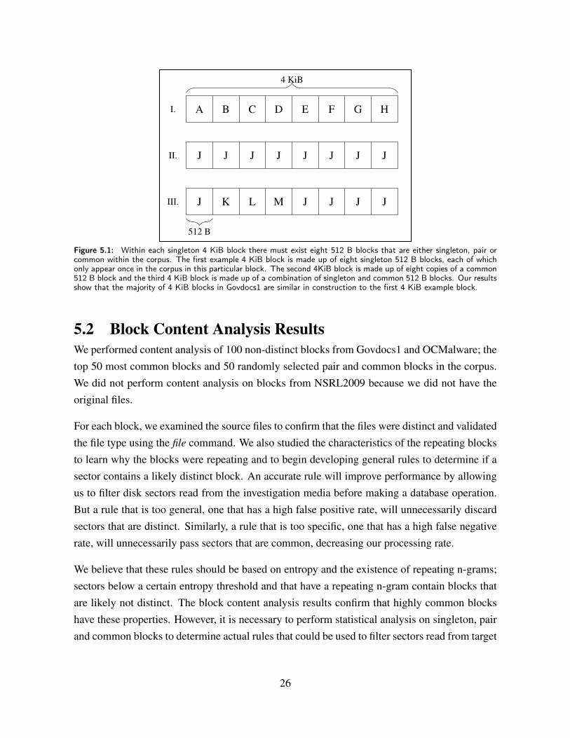
We also found a similar percentage of singletons for the 512 B and 4 KiB block sizes forGovdocs1 and OCMalware. Each 4 KiB singleton block consists of a combination of eight512 B blocks that are either singleton, pair or common, as illustrated in Figure 5.1. Since thepercentages of singletons for both block sizes are similar, we conclude that most of the 4 KiBsingleton blocks are made up of eight singleton 512 B blocks and we do not loose granularityby choosing a larger block size. For the remainder of this chapter, we discuss the properties ofthe 4 KiB blocks from each corpus unless otherwise noted.

25

I.

II.

III.

A B C D E F G H

4 KiB

J J J J J J J J

J K L M J J J J

512 B

Figure 5.1: Within each singleton 4 KiB block there must exist eight 512 B blocks that are either singleton, pair orcommon within the corpus. The first example 4 KiB block is made up of eight singleton 512 B blocks, each of whichonly appear once in the corpus in this particular block. The second 4KiB block is made up of eight copies of a common512 B block and the third 4 KiB block is made up of a combination of singleton and common 512 B blocks. Our resultsshow that the majority of 4 KiB blocks in Govdocs1 are similar in construction to the first 4 KiB example block.

5.2 Block Content Analysis ResultsWe performed content analysis of 100 non-distinct blocks from Govdocs1 and OCMalware; thetop 50 most common blocks and 50 randomly selected pair and common blocks in the corpus.We did not perform content analysis on blocks from NSRL2009 because we did not have theoriginal files.

For each block, we examined the source files to confirm that the files were distinct and validatedthe file type using the file command. We also studied the characteristics of the repeating blocksto learn why the blocks were repeating and to begin developing general rules to determine if asector contains a likely distinct block. An accurate rule will improve performance by allowingus to filter disk sectors read from the investigation media before making a database operation.But a rule that is too general, one that has a high false positive rate, will unnecessarily discardsectors that are distinct. Similarly, a rule that is too specific, one that has a high false negativerate, will unnecessarily pass sectors that are common, decreasing our processing rate.

We believe that these rules should be based on entropy and the existence of repeating n-grams;sectors below a certain entropy threshold and that have a repeating n-gram contain blocks thatare likely not distinct. The block content analysis results confirm that highly common blockshave these properties. However, it is necessary to perform statistical analysis on singleton, pairand common blocks to determine actual rules that could be used to filter sectors read from target

26

Govdocs1 Frequency Number of Number of Entropy Pattern DescriptionBlock Ranking Files File Types Size (Bytes)1 88,503 5,079 5 0 1 NUL block (0x00)2 59,250 2,996 5 0 1 All 1s (0xFF)3-22* 10,634 2,400 1 2.3 20 Adobe Acrobat XREF Table23 6,437 23 1 1 2 TIFF structure24-28, 30-34* 2,996 2,996 1 3.3 n/a Compound Document SAT29, 35-36, 40* 2,934 274 4 2 4 JFIF structure37-39, 41-50* 2,996 2,996 1 3.3 n/a Compound Document SAT

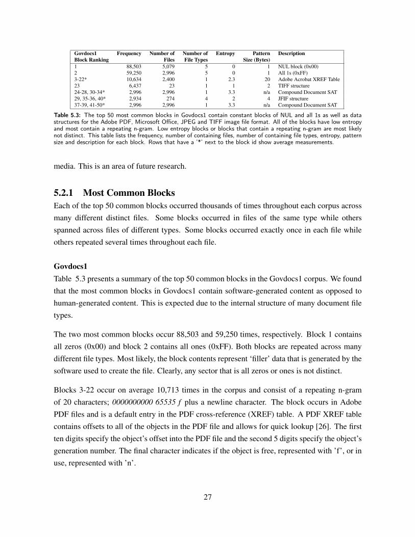
Table 5.3: The top 50 most common blocks in Govdocs1 contain constant blocks of NUL and all 1s as well as datastructures for the Adobe PDF, Microsoft Office, JPEG and TIFF image file format. All of the blocks have low entropyand most contain a repeating n-gram. Low entropy blocks or blocks that contain a repeating n-gram are most likelynot distinct. This table lists the frequency, number of containing files, number of containing file types, entropy, patternsize and description for each block. Rows that have a ’*’ next to the block id show average measurements.

media. This is an area of future research.

5.2.1 Most Common BlocksEach of the top 50 common blocks occurred thousands of times throughout each corpus acrossmany different distinct files. Some blocks occurred in files of the same type while othersspanned across files of different types. Some blocks occurred exactly once in each file whileothers repeated several times throughout each file.

Govdocs1Table 5.3 presents a summary of the top 50 common blocks in the Govdocs1 corpus. We foundthat the most common blocks in Govdocs1 contain software-generated content as opposed tohuman-generated content. This is expected due to the internal structure of many document filetypes.

The two most common blocks occur 88,503 and 59,250 times, respectively. Block 1 containsall zeros (0x00) and block 2 contains all ones (0xFF). Both blocks are repeated across manydifferent file types. Most likely, the block contents represent ‘filler’ data that is generated by thesoftware used to create the file. Clearly, any sector that is all zeros or ones is not distinct.

Blocks 3-22 occur on average 10,713 times in the corpus and consist of a repeating n-gramof 20 characters; 0000000000 65535 f plus a newline character. The block occurs in AdobePDF files and is a default entry in the PDF cross-reference (XREF) table. A PDF XREF tablecontains offsets to all of the objects in the PDF file and allows for quick lookup [26]. The firstten digits specify the object’s offset into the PDF file and the second 5 digits specify the object’sgeneration number. The final character indicates if the object is free, represented with ’f’, or inuse, represented with ’n’.

27

Block 23 occurred 6,437 times in the corpus and consisted of a repeating n-gram of 2 char-acters, 0xFF 00. This block occurs in embedded Tagged Image File Format (TIFF) images inEncapsulated PostScript (EPS) files.

Repeating n-grams are clearly not distinct because they are too common. There are only 256(28) different blocks that contain a repeating uni-gram. The probability that two randomlygenerated repeating uni-gram blocks match is 1 in 256, 0.3%. Similarly the probability fortwo 2-gram blocks is 1 in 65 K (216), the probability for 3-gram blocks is 1 in 16 M (224) andso on. The probability that two repeating 20-gram blocks match is 1 in 2160, highly unlikely.However, we find that the Adobe default XREF entry, a 20-gram, is very common in Govdocs1.This block occurs more frequently then expected because it is a standard block generated bythe Adobe software. There are many other common repeating n-gram blocks in Govdocs1 thatare software generated and make up a portion of the file format internal structure. Our resultssupport our proposed rule-of-thumb that if a block contains a repeating n-gram, it is likely notdistinct.

Blocks 24-28, 30-34, 37-39 and 41-50 occur on average 2,996 times in the corpus in MicrosoftOffice documents. The blocks have low entropy but do not consist of a repeating n-gram.The blocks are from the Microsoft Compound Document File Format Sector Allocation Table(SAT). The SAT is an array of Sector IDs (SecIDs), a 4-byte value, that list the internal filesectors where user streams are stored in the document [27].

Each entry in the SAT lists the index of the next SecID in the chain or a special reserved valuethat provides meta-information about the chain. For example, a SAT stored in little-endian orderthat has 0x01 00 00 00 at index 0, 0x02 00 00 00 and index 1, 0x03 00 00 00 at index 2, and0xFE FF FF FF at index 3, indicates that a user stream is stored in sectors 0 - 3 and that 3 isthe last sector in the chain (a SecID value of -2 indicates that the sector is the last in the chain).A hexdump of three sample blocks with different SecID arrays is shown in Figure 5.2.

Blocks 29, 35-36 and 40 occur on average 2,934 times in the corpus in embedded JPEG files invarious container files. Each block consists of a repeating 4-gram pattern 0x28 A2 80 0A. Thefirst occurrence of each block is preceded by a JPEG File Interchange Format (JFIF) Header.The header began with a Start of Image (SOI) marker, (0xFF D8), followed by the JFIF Ap-plication Use (APP0) marker, (0xFF E0) in the Microsoft Office, JPEG and Macromedia Flashfiles and (0xFF EE) in the Adobe Acrobat files [28, 29]. The JFIF header in the Microsoft Of-fice, JPEG and Macromedia Flash files also contained the identifier “JFIF”, (0x4A 46 49 46

28

Block 26 - Sector Allocation Table(SAT)

00000000 01 00 00 00 02 00 00 00 03 00 00 00 04 00 00 00 0000000010 05 00 00 00 06 00 00 00 07 00 00 00 08 00 00 00 0000000020 09 00 00 00 0a 00 00 00 0b 00 00 00 0c 00 00 00 0000000030 0d 00 00 00 0e 00 00 00 0f 00 00 00 10 00 00 00 0000000040 11 00 00 00 12 00 00 00 13 00 00 00 14 00 00 00 00

Block 31 - SAT

00000000 01 02 00 00 02 02 00 00 03 02 00 00 04 02 00 00 0000000010 05 02 00 00 06 02 00 00 07 02 00 00 08 02 00 00 0000000020 09 02 00 00 0a 02 00 00 0b 02 00 00 0c 02 00 00 0000000030 0d 02 00 00 0e 02 00 00 0f 02 00 00 10 02 00 00 0000000040 11 02 00 00 12 02 00 00 13 02 00 00 14 02 00 00 00

Block 32 - SAT

00000000 81 02 00 00 82 02 00 00 83 02 00 00 84 02 00 00 0000000010 85 02 00 00 86 02 00 00 87 02 00 00 88 02 00 00 0000000020 89 02 00 00 8a 02 00 00 8b 02 00 00 8c 02 00 00 0000000030 8d 02 00 00 8e 02 00 00 8f 02 00 00 90 02 00 00 0000000040 91 02 00 00 92 02 00 00 93 02 00 00 94 02 00 00 00

Figure 5.2: Govdocs1 blocks 24-28, 30-34, 37-39 and 41-50 were found in the Compound Document File Format SectorAllocation Table (SAT) and contain an array of 4-byte Sector IDs (SecIDs) that list the sectors that user streams arestored in. This diagram shows the first 80 bytes of three sample blocks with different arrays of SecIDs.

JFIF Header in Microsoft Power Point files

00000000 ff d8 ff e0 00 10 4a 46 49 46 00 01 01 01 01 2c |......JFIF.....,|00000010 01 2c 00 00 ff db 00 43 00 08 06 06 07 06 05 08 |.,.....C........|00000020 07 07 07 09 09 08 0a 0c 14 0d 0c 0b 0b 0c 19 12 |................|00000030 13 0f 14 1d 1a 1f 1e 1d 1a 1c 1c 20 24 2e 27 20 |........... $.’ |00000040 22 2c 23 1c 1c 28 37 29 2c 30 31 34 34 34 1f 27 |‘‘,#..(7),01444.’|

JFIF Header in Adobe Acrobat files

00000000 ff d8 ff ee 00 0e 41 64 6f 62 65 00 64 00 00 00 |......Adobe.d...|00000010 00 01 ff db 00 43 00 0e 0a 0b 0d 0b 09 0e 0d 0c |.....C..........|00000020 0d 10 0f 0e 11 16 24 17 16 14 14 16 2c 20 21 1a |......$....., !.|00000030 24 34 2e 37 36 33 2e 32 32 3a 41 53 46 3a 3d 4e |$4.763.22:ASF:=N|00000040 3e 32 32 48 62 49 4e 56 58 5d 5e 5d 38 45 66 6d |>22HbINVX]^]8Efm|

Figure 5.3: Many of the Govdocs1 common blocks are in embedded JPEG images. This diagram shows the first 80bytes of the JFIF header in the block proceeding the instance of Block 29 in two file types. The JFIF header in aMicrosoft Power Point file starts with (0xFF D8 FF E0) and includes the string ”JFIF” . Note that the ASCII characterat position 0x40 in the Microsoft Power Point JFIF header is the straight double quote character (0x22). The JFIFheader in an Adobe Acrobat file starts with (0xFF D8 FF EE).

00) [30]. Figure 5.3 shows a hexdump of both headers.

OCMalwareThe top 50 common blocks in OCMalware have various types of content. We did not reverseengineer any of the malware samples because it is outside of the scope for this thesis. Wegenerally determined block functions by statically analyzing the content when appropriate andcomparing the malware blocks to other blocks from known files in the NSRL2009–we computed

29

the SHA-1 of the top 50 common 4 KiB malware blocks to compare to NSRL2009.

Similar to the common blocks of Govdocs1, there are many occurrences of the NUL blockand the uni-gram block with all 1s, the first and fourth most common blocks in the corpus,respectively.

Block 2 occurs 741,084 times and consists of a repeating uni-gram, 0x90. The majority of thefiles that have block 2 are PE32 Executables for Intel x86 machines and the block was not foundin the NSRL2009. The hex value 0x90 is the Intel x86 No Operation (NOOP) instruction thathas no effect on the machine context but advances the instruction pointer [31]. A sequenceof NOOP instructions is often used to pad the area around a target instruction when the exactlocation of the instruction is unknown. If the execution flow reaches the NOOP sequence, thenthe instruction pointer will ‘slide’ to the target location. NOOP slides are often used in bufferoverflows and similar exploits [32].

We suspect that block 2 is a NOOP slide due to the nature of the files in OCMalware, but itwould require additional analysis of each containing file to confirm the block’s function.

Block 3 occurs 7,022 times and consists of a repeating uni-gram, 0x2E. All of the containingfiles are PE32 executables. However, there is no 1-byte Intel x86 instruction with that value.This block matches blocks in NSRL2009. All of the containing NSRL files have file extensionsfor image file formats (i.e. JPG, GIF). The hex value 0x2E 2E 2E is the RGB value for darkgray. Block 3 is probably included in the data portion of the executable and may contain anembedded image.

Blocks 5-50 occur on average 114,999 times and have high entropy of 7.22. The blocks occurat the same offset in the containing files. For example, block 5 occurs at offset 4,096 in 125,025unique files: each file has a unique MD5 hash and file size. A sample of the containing filesare as reported by VirusTotal.com, a free virus, malware and URL online scanning service [25].VirusTotal.com compares hashes to 40 antivirus signature sets and identifies matching malwareinstances. The sampled file hashes match different variants of the YahLover Worm, a low riskvirus that enumerates system files and directories [33].

All 46 high entropy common blocks occur in the same 125,000 files. Each file is 255 KiB, onaverage and the first 60 4 KiB blocks occur in each file at the same offset. The blocks don’tmatch any blocks in NSRL so we know that the blocks are specific to these malware samples.We suspect that all of these files are variants of the YahLover worm and that the files were

30

OCMalware Frequency Number of Entropy Pattern DescriptionBlock Ranging Files Size (Bytes)1 13,396,994 547,662 0 1 NUL block (0x00)2 741,084 7,022 0 1 Repeating n-gram block (0x90)3 218,134 1,330 0 1 Repeating n-gram block (0x2E)4 133,492 4,662 0 1 All 1s (0xFF)5-50* 114,999 114,999 7.22 N/A Blocks from variants

of the same malware sample

Table 5.4: The top 50 most common blocks in OCMalware include four repeating uni-grams and 46 high-entropyblocks. The repeating uni-grams are the NUL block, the block of all ones, a potential NOOP slide and data blockthat matches image files in the NSRL2009. The high-entropy blocks occur exclusively in variants of a malware sample.This block can help identify other variants of the same file. This table lists the frequency, number of containing files,entropy, pattern size and description for each block. Rows that have a ’*’ next to the block id show average values.

slightly modified by adding bytes to the end of the file. The modifications change the file hashwhich would prevent detection by antivirus scanners but not the block hashes as demonstratedby our findings.

This is an important finding because the common blocks are distinct to a specific malwaresample and can be used to find other variants of the malware. Other malware samples mayshare blocks as a result of hand-patching existing malware and code reuse.

5.2.2 Random Pair and Common BlocksWe analyzed 50 random pair and common blocks in Govdocs1. The common blocks occurbetween three and five times in the corpus. We call these blocks low-occurrence blocks becausethey are repeated in the corpus but not often. The results of our analysis show that many of thelow-occurrence blocks occur in files that are extremely similar and have many of their blocks incommon. This occurs when files are copied and modified, created using the same template, orembedded into the same files. In the case of Govdocs1, they maybe a result of the acquisitionmethodology. These blocks are not distinct according to our definition but in some cases canbe used to identify a class of content, similar to how the high entropy malware blocks identifyother variants of the same malware.

Other low-occurrence blocks occur in files that only share a few blocks in common and the filesare visually distinct. It is not clear why the block is repeated in this instance. It could occur dueto a similarity in internal file structure or a small shared embedded file–for example, a sharedembedded font. No general conclusion as to the root cause of these blocks was identified.

The following subsection describes the types of low-occurrence blocks seen in Govdocs1.

31

5.2.3 Findings

Analysis of the 50 random low-occurrence blocks in Govdocs1 is summarized in Table 5.5.The containing files as named in the Govdocs1 corpus are listed. The blocks occur in files ofthe same type or in the same file. Most of the blocks have high entropy although there areoccurrences of low entropy blocks and one block has a repeating n-gram.

Blocks 51-90 occur in files that are nearly identical sharing almost all blocks in common exceptfor the first and last block, files with revisions of the same content, files that use the sametemplate and embedded files. All such files share the majority of their blocks in common at thesame offset.

Nearly identical files have similar file sizes and all of the blocks are identical except for thetrailing block. The blocks only occur in these files throughout the corpus and and there areinstances of high and low entropy blocks. For example block 51 occurs in two visually identicalPDF files that have 100% of their full blocks in common.

Files with revisions of the same content have file meta-data that indicates as such. We visuallyinspected the files to confirm that the contents were very similar. These blocks occur at the sameoffset, generally have high entropy and are only common to the containing files. For example,block 72 occurs in two Microsoft Power Point files that have the same creation date, authorand title. The first file, 208098.ppt, is labeled as revision 155 and was last saved in September2005 and the second file, 723019.ppt, is revision 164 and was last saved 22 days later. Bothpresentations have similar content and visual style; 96% of the blocks in 208098.ppt are pairblocks that only repeat in the 723019.ppt.

Files that use the same Microsoft Word or Power Point template share many blocks in common.These blocks have high entropy and occur at the same offset. For example, block 74 occurredin two Power Point Files that were different sizes, created and edited by different users, haddifferent content but both use the Focused senses design template indicated in the file meta-data. The Power Point files share 76 blocks that only occur in these two files.

Files that share embedded content contain the same embedded file. For example, block 78occurs in 161839.ppt and 235468.ppt, two Microsoft Power Point presentations with differentcontent and style. However, both presentations have an embedded PNG image of a governmentagency logo. Block 78 is one of 20 pair blocks that make up the PNG image.

32

All of the similar blocks, except for the template blocks, can be used to identify similar files;files that have different variants of the same content. Blocks that contain Microsoft Templatescan be automatically identified using the NSRL RDS.

Each of the similar files has a unique file hash that would prevent identifying the similarityusing file hashing. However, Roussev’s similarity digest would rate these files as having sharedcontent [34].

Blocks 91-95 only occur in the same file. For example, block 91 occurs in a log file with ASCIItext. The block occurs twice in the file and contains the same lines of log date. The repeatedblocks have low entropy. These blocks are distinct according to our definition because the repeatblock occurrence happens in the same file. Since the block is not repeated in any other file, itcan be used to identify a specific file.

Blocks 96-100 occur in different files of the same type that have different sizes and meta dataand appear visually distinct and unrelated. For example, block 100 is high entropy and appearsin two PDF files at different offsets. The files are mostly text and contain different content.The first file, 322064.pdf, is 2 pages long and contains text and an image of a United Statesmap. The second file, 134635.pdf, is 24 pages and contains all text. The files share 94 blocksin common, more than 55% for each file, and the blocks are contiguous in each file.

It is not clear why these documents share so many blocks in common. If the blocks are specificto PDF files, then we would expect to see more instances occur in other PDF files throughoutthe corpus. Perhaps we would find more instances with a larger corpus or perhaps the blocksidentify a specific computer that was used to create the file.

5.3 Initial Statistical Analysis of Block TypesAs illustrated in Table 5.6, the singleton blocks have the highest average entropy, the lowestpercentage of repeating n-grams blocks and the highest average n-gram pattern size. The com-mon blocks have the lowest average entropy, the largest percentage of repeating n-gram blocksand the lowest average n-gram pattern size. This is not surprising because we expect blockswith high entropy to appear less frequently in the corpus than blocks with low entropy. We alsoexpect longer patterns to appear less frequently then shorter patterns because there are more bitsof entropy in the former.

Based on our analysis of the most common and low-occurrence blocks in Govdocs1 and OC-

33

Malware, we believe that any sector that has low entropy or a repeating n-gram is likely not dis-tinct. If most files contain distinct blocks, then filtering sectors with likely non-distinct blockswill allow us to identify files and minimize the number of database operations. Additionalanalysis is required to affirm this hypothesis and determine an appropriate entropy threshold.

34

Govdocs1 Frequency Entropy N-gram File File ContainingBlock Size Type Relation FilesRanking (Bytes)Blocks Repeated in Similar Files51 2 7.85 PDF Nearly Identical 398395.pdf 635062.pdf52 2 5.45 TEXT Nearly Identical 103501.html 186235.text53 4 7.35 PDF Nearly Identical 883566.pdf 883682.pdf

887380.pdf 902600.pdf54 2 7.92 PPT Revisions 400527.ppt 816306.ppt55 2 7.78 PPT Revisions 737795.ppt 831305.ppt56 2 7.88 PPT Revisions 125596.ppt 344997.ppt57 2 7.92 PPT Revisions 716143.ppt 896918.ppt58 2 7.63 PPT Revisions 823851.ppt 823850.ppt59 2 7.95 PPT Revisions 081192.ppt 222426.ppt60 2 6.64 PPT Revisions 060050.ppt 733179.ppt61 2 7.96 PPT Revisions 265577.ppt 718449.ppt62 2 7.92 PPT Revisions 520238.ppt 520257.ppt63 2 7.85 PPT Revisions 759319.ppt 930569.ppt64 2 7.60 PPT Revisions 470989.ppt 720950.ppt65 2 3.59 PPT Revisions 153678.ppt 158011.ppt66 2 7.49 PPT Revisions 219463.ppt 499297.ppt67 2 3.61 PPT Revisions 148699.ppt 470007.ppt68 2 7.95 PPT Revisions 550550.ppt 729042.ppt69 2 7.91 PPT Revisions 223916.ppt 432439.ppt70 2 7.93 PPT Revisions 852904.ppt 877644.ppt71 2 7.94 PPT Revisions 328305.ppt 769590.ppt72 2 5.53 PPT Revisions 208098.ppt 723019.ppt73 2 7.88 PPT Revisions 251761.ppt 251763.ppt74 2 7.84 PPT Common Template 064978.ppt 064978.ppt75 2 7.92 PPT Common Template 113862.ppt 113862.ppt76 4 7.89 WORD Common Template 328908.doc 448441.doc

510693.doc 552838.doc77 5 1.675 18 WORD Common Template 128593.doc 134249.doc

260394.doc 779316.doc944415.doc

78 2 7.95 PPT Embedded Image 161839.ppt 235468.ppt79 2 0.96 PS Similar 265414.ps 310640.ps80 2 7.95 WORD Similar 497046.doc 541565.doc81 2 0.52 WORD Similar 042097.doc 215070.doc82 2 7.95 PDF Similar 153927.pdf 512812.pdf83 2 7.95 PPT Similar 514540.ppt 876566.ppt84 2 7.91 PDF Similar 785678.pdf 823177.html85 2 3.58 PPT Similar 582372.ppt 593079.ppt86 2 1.43 PS Similar 265414.ps 310640.ps87 2 4.05 PS Similar 144630.ps 742084.ps88 2 5.42 HTML Similar 564700.html 844361.html89 2 5.06 XML Similar 370547.xml 649858.xml90 3 1.43 XLS Similar 675701.xls 677169.xls

688704.xls

Blocks Repeated in the Same File91 3 1.76 WORD Same file 051904.doc92 2 2.25 PPT Same file 656483.ppt93 2 4.29 WORD Same file 900384.doc94 2 4.62 TXT Same file 108573.log95 2 2.94 PS Same file 974311.ps

Blocks Repeated in Dissimilar Files96 2 7.95 PDF Dissimilar 036978.pdf 698843.pdf97 2 7.96 PDF Dissimilar 503976.pdf 895665.pdf98 2 7.95 PDF Dissimilar 302985.pdf 321983.pdf99 2 7.93 PDF Dissimilar 630279.pdf 927000.pdf100 2 7.94 PDF Dissimilar 134635.pdf 322064.pdf

Table 5.5: Fifty random low-occurrence blocks in Govdocs1 occurred in a few files in the corpus and no where else.Some of the containing files were similar, sharing a large percentage of pair or common blocks and containing similarcontent. Special types of similar files include nearly identical files, files with revisions of the same content, files thatshared a common template and files that shared embedded content. Other blocks repeated in the same file and stillother blocks occurred in dissimilar files where there was no perceived similarity in content or file metadata. It is unclearwhy blocks repeat in dissimilar files although our results show that this scenario does occur.

35

Measurement Singleton Pair CommonAverage entropy (per byte) 6.68 6.61 5.52Standard deviation 1.92 0.34 2.70Percentage of blocks that contain repeating n-grams 0.12 0.48 10.62Avgerage n-gram size (bytes) 755 557 315Standard deviation 33 56 170

Table 5.6: The entropy and n-gram statistics for singleton, pair and common blocks in Govdocs1. As expected thesingleton blocks have the highest average entropy and the common blocks have the highest percentage of repeatingn-gram blocks with the shortest average n-gram size.

36

CHAPTER 6:Data Storage Experiment

Deploying sector hashing for full media analysis and sampling strongly requires a high perfor-mance database. The database must be able to store the file block hashes of every file that wehave ever seen be fast enough to support triage at disk I/O speed. Previously published sec-tor hashing methods do not scale for this number of files [10, 12]. It is critical therefore thatour application supports both a large and fast database to leverage the intelligence from manyprevious investigations instead of just a few target files.

A database with 1 billion hashes will support a sufficient amount of content for many applica-tions. One billion (109) 512 B block hashes can reference 1 billion 512 B file blocks, which is512 GB of known content, which is large enough to store each of the corpora analyzed in thisthesis. Similarly, 1 billion 4 KiB block hashes can reference 4 TB of known content, which islarger than the collection of known child pornography at the National Center for Missing andExploited Children [35].

Today, we can read a 1 TB (1012) hard drive in 200 minutes at maximum I/O transfer rate [7].A 1 TB hard drive has 2 billion 512 B sectors and therefore a maximum sector reading rate of150 K sectors/second. Assuming that hashing is free, the disk sector hashes are available tocompare to the file block hash database at the same rate. Therefore the database must support aquery rate of 150 K lookups per second for full media analysis.

With media sampling the required rates are not as high. As discussed in Chapter 1, sampling just1 million randomly chosen disk sectors can identify 4 MB of content with 98.17% probability,provided that each of the 8,000 content blocks are distinct. A 7200 RPM hard drive can performapproximately 300 seeks per second. If pre-sorted it is possible to read 1 million randomlychosen sectors in 30 minutes on most systems today. Thus, for the random sampling application,a database query rate of a few thousand transactions per second is sufficient [7].

Our goal for the data storage experiment is to determine if we can achieve sufficient databasequery rates to support media sampling.

37

6.1 PurposeThe purpose of this experiment is to determine the relative performance of several generalpurpose SQL and NoSQL database management systems (DBMS) for storing and performingqueries on a large file block hash database.

A general purpose DBMS is typically designed to meet many usage requirements including dataaccuracy and availability, resilience to errors and loss, simultaneous read and write access bymultiple users and enterprise scalability [36–39]. The usage requirements for the hash databaseare not as broad. The database is essentially a key-value store where the key is a cryptographichash of the file block and the value is a file identification number and byte offset where theblock occurs. For the single-system field-deployed usage model, the database will rarely beupdated, and run on a single laptop accessed by one or few connections. The most criticalusage requirement is that the DBMS can perform fast queries for a database with one billionrows. To our knowledge, there are no previous benchmark tests that focuses on the specificusage requirements of full media analysis with sector hashing.

We used standard configuration options for each DBMS to measure the database query per-formance. No external pre-filtering was performed, such as using a bloom filter to distinguishbetween queries of absent and likely present hashes in the database. However, the results in Ta-ble 7.1 suggest that the DBMSs use their own pre-filtering since absent queries are performedat a faster rate then present queries.

6.2 MethodologyWe tested the performance of three SQL DBMSs: MySQL, postgreSQL and SQLite, and oneNoSQL DBMS: MongoDB. We used the latest software at the time of our study as shown inTable 6.2. For each DBMS, we built four databases that contain a single table of 1 million,10 million, 100 million or 1 billion rows. We performed hash query tests on the databases todetermine the performance of all DBMSs. Note that in the MongoDB DBMS, tables are calledcollections and rows are called documents [40]. We use the terms table and row generallyfor all DBMSs. Since each database only has one table, we use the terms database and table

interchangeably.

The experiment is separated into several steps described in the following discussion.

First, we generated the file block hash data and save it in tab-delimited plain-text files. There

38

897316929176464ebc9ad085f31e7284 0 0b026324c6904b2a9cb4b88d6d61c81d1 1 126ab0db90d72e28ad0ba1e22ee510510 2 26d7fce9fee471194aa8b5b6e47267f03 3 348a24b70a0b376535542b996af517398 4 41dcca23355272056f04fe8bf20edfce0 5 59ae0ea9e3c9c6e1b9b6252c8395efdc1 6 684bc3da1b3e33a18e8d5e1bdd7a18d7a 7 7c30f7472766d25af1dc80b3ffc9a58c7 8 87c5aba41f53293b712fd86d08ed5b36e 9 9

Figure 6.1: The data shown is the first ten lines of a hash data file. We created 12 hash data files for each database.The first column in the file is an MD5 hash, the second is a fileid identification number and the third is a byteoffset. The first line represents a block from file 0 at byte offset 0 (the start of the file) with a MD5 hash of897316929176464ebc9ad085f31e7284. The files were used to bulk load data into the databases, the fastest loadmethod for each DBMS.

are twelve data files in total; one for each of the 1 million, 10 million and 100 million rowdatabases and ten for the 1 billion row database – the billion row database is split into ten datafiles of 100 K rows, one of which is the data file for the 100 million row database. Each rowin a data file corresponds to a row in the database and contains information for a file block; anMD5 hash, file identification number, and byte offset as shown in Figure 6.1.

We chose to pre-generate the data as opposed to generating it at load time because file bulkloading is the fastest way to populate databases and each DBMS supports data loading from acomma or tab-separated file. Additionally, pre-generating the data prevents work duplicationwhen loading multiple instances of the same database stored in different DBMSs. Anothermethod for avoiding duplication is to build the database in one DBMS, query the data and loadit into all other DBMSs. Although this would prevent storing the data in an additional format,the method is not as efficient as loading from a file.

Next, we created the database and the schema defining the columns in each row and the data type

of each column. There are three columns in each table, hash, fileid and offset that correspond tothe file block data as previously described. The data schema is discussed in detail in Section 6.3.The database creation commands that define the schema are listed in Table 6.1.

All the DBMSs support a database index, a search data structure created from a column inthe database that significantly improves performance of queries on data stored in the indexedcolumn. Without an index, each query is compared to every row in the database. Using anindex causes slower write times because the index structure is dynamically built when the datais inserted. Building the index after all the data is written to the database allows for both fast

39

MySQL InnoDB:

create table hashes (hash char(32), fileid integer, offset integer) engine=innodb

MySQL MyISAM:

create table hashes (hash char(32), fileid integer, offset integer) engine=innodb

PostgreSQL:

create table hashes (hash char(32), fileid integer, offset integer)

SQLite:

create table hashes (hash text, fileid int, offset int)

MongoDB:

d[hashes]

Table 6.1: These DBMS commands create a hash database with columns hash, fileid and offset, a MD5 hash,file identification number and byte offset, respectively. A detailed discussion of the database schema is provided inSection 6.3. Note that MongoDB does not take column names or types when creating the database. The columnnames are provided on data insert and the type is dynamically determined to best fit the data.

write times and query times. It is also better to build the index from a fully populated databaseto ensure that it is well structured and will provide optimal search performance [41]. Therefore,the database index is not created until after the data are loaded.

Third, we loaded the database by performing a bulk load from the data file as previously dis-cussed. After the data is successfully loaded, we build the database index from the hash column.Since we query the database to find matching file block hashes from the disk sectors, the hash

column is an obvious choice for the index.

Finally, we ran a series of timed database query tests. We created a Python software test toolthat connects to a database and performs queries for present or absent values, hash values thatexist or do not exist in the database, respectively. Python supports modules for each DBMSas shown in Table 6.2. We discuss the algorithm to determine present and absent hashes inSection 6.3.

During each test, queries for either present or absent hashes are performed exclusively for afixed amount of time. We measured the number of completed queries and the time to completeeach query. We chose to take measurements after each query to eliminate the time taken on the

40

Database Python3 ModuleMySQL 5.5.22 pymysql 0.5PostgreSQL 9.1.3 psycopg2 2.4.5SQLite 3.7.7.1 sqlite3 2.6.0MongoDB 2.0.4 pymongo 1.9b1

Table 6.2: We used the latest versions of database software and the corresponding Python3 module. We built thebinaries for MySQL, PostgreSQL, MongoDB and pymysql. All other binaries were acquired from a Fedora 16 packagerepository.

other portions of the Python program. The total time is calculated as the sum of the individualquery times. Although measuring this frequently adds to the overhead of the program, we foundthat the majority of the allotted query time was spent actually accessing the database. Due toour access method, the time measurements include the execution time for the Python databasemodule and for network interaction except for SQLite, which does not use a client/server model.

When searching a target disk, we expect that most of the disk sectors will not match the distinctblocks in our hash database because we do not expect all of the known-files to exist on one disk.Therefore, we are especially interested in the query rate for absent values.

Caching is used by all DBMSs to store recently accessed portions of the database and index–either with an internal cache or the Operating System file system cache. We clear all cachesbefore a run of the experiment to start with a cold cache and run each test long enough toachieve a steady query rate with a hot cache. A cold cache is empty and does not contain anyportions of the database. Handling a new query with a cold cache requires reading from thedisk to access the corresponding portion of the database and storing the portion in the cache forfuture access. A hot cache contains portions of the database and there is a higher probabilitythat a new query corresponds to a portion of the database in the cache, preventing a costlydisk access. We discuss in Sections 6.5 and 6.6 the configuration settings to clear the internaldatabase cache and Operating System cache, respectively.

We performed the experiments on a Dell R510 server equipped with Dual Xeon E5620 2.4Ghzprocessors (16 core, 12 MiB cache, 128 GiB main memory). The server ran a 64 bit versionof Fedora 16 with Linux kernel 3.4.2-1.fc16.x86_64. The databases were stored on a 21 TBphysical RAID partition running XFS, a high-performance journaling file system for 64 bitarchitectures [42].

41

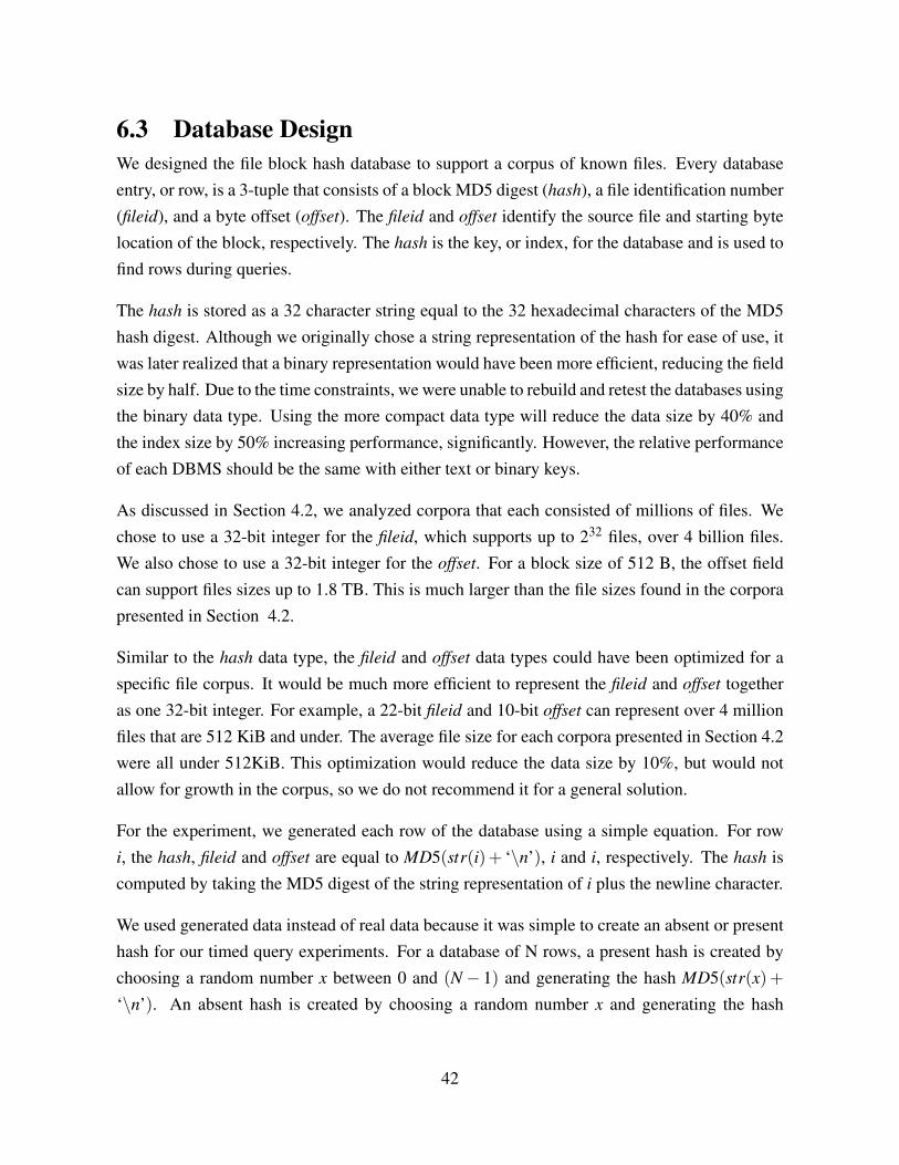
6.3 Database DesignWe designed the file block hash database to support a corpus of known files. Every databaseentry, or row, is a 3-tuple that consists of a block MD5 digest (hash), a file identification number(fileid), and a byte offset (offset). The fileid and offset identify the source file and starting bytelocation of the block, respectively. The hash is the key, or index, for the database and is used tofind rows during queries.

The hash is stored as a 32 character string equal to the 32 hexadecimal characters of the MD5hash digest. Although we originally chose a string representation of the hash for ease of use, itwas later realized that a binary representation would have been more efficient, reducing the fieldsize by half. Due to the time constraints, we were unable to rebuild and retest the databases usingthe binary data type. Using the more compact data type will reduce the data size by 40% andthe index size by 50% increasing performance, significantly. However, the relative performanceof each DBMS should be the same with either text or binary keys.

As discussed in Section 4.2, we analyzed corpora that each consisted of millions of files. Wechose to use a 32-bit integer for the fileid, which supports up to 232 files, over 4 billion files.We also chose to use a 32-bit integer for the offset. For a block size of 512 B, the offset fieldcan support files sizes up to 1.8 TB. This is much larger than the file sizes found in the corporapresented in Section 4.2.

Similar to the hash data type, the fileid and offset data types could have been optimized for aspecific file corpus. It would be much more efficient to represent the fileid and offset togetheras one 32-bit integer. For example, a 22-bit fileid and 10-bit offset can represent over 4 millionfiles that are 512 KiB and under. The average file size for each corpora presented in Section 4.2were all under 512KiB. This optimization would reduce the data size by 10%, but would notallow for growth in the corpus, so we do not recommend it for a general solution.

For the experiment, we generated each row of the database using a simple equation. For rowi, the hash, fileid and offset are equal to MD5(str(i)+ ‘\n’), i and i, respectively. The hash iscomputed by taking the MD5 digest of the string representation of i plus the newline character.

We used generated data instead of real data because it was simple to create an absent or presenthash for our timed query experiments. For a database of N rows, a present hash is created bychoosing a random number x between 0 and (N− 1) and generating the hash MD5(str(x)+‘\n’). An absent hash is created by choosing a random number x and generating the hash

42

Database Schema TermsTerm DefinitionN The number of rows in a database.Fi A unique identifier for the ith file in the corpus.o A byte offset.Fo

i The fixed-size block at offset o in Fi.str(x) The string representation of x.MD5(y) The 32 hexadecimal digits of the MD5 digest of y.

Database Schema DescriptionColumn Size Experimental Value Actual Valuefileid 32 bits n ∈ 0...(N−1) Fioffset 32 bits n ∈ 0...(N−1) ohash 256 bits str(MD5(str(n)+ ‘\n’)) MD5(Fo

i )

Table 6.3: Each entry in the file block hash database is a 3-tuple (hash,fileid,offset). The hash is the 32 MD5hexadecimal characters (256 bits) of a block that exists in a file represented by a unique fileid at a specific byte offset.We list the experiment values that were used generated for the experiment. The values differ from the listed actualvalues that will be used for a real block hash database. The summary of each value and its size is listed for a databaseof N rows.

MD5(str(x)+ ‘x’). By definition, the former value is in the database while the latter is not.Furthermore, since hashes are evenly distributed, our generated data has a similar distributionto the block hashes of actual files.

Table 6.3 summarizes the entries for the generated hash database used during the experimentand for the real hash database that will be created from a corpus of known files.

6.4 DBMS OverviewMySQL is advertised as the world’s most used open source Relational Databases ManagementSystem (RDBMS) [43]. The software uses a client/server model and supports several back-enddata storage engines for each table in a database [44]. One of the advantages of using MySQLis the flexibility of choosing the storage engine and optimizing a table for a specific use [45].

We measured the performance of the InnoDB and MyISAM storage engines. InnoDB is thedefault storage engine for MySQL version 5.5.5 and later and is best suited for write heavyenvironments where data reliability is most critical. MyISAM is the default storage enginefor MySQL versions earlier than 5.5.5 and has high performance for read heavy environmentswhere the data are not frequently updated [44, 45].

Both InnoDB and MyISAM support table indexing and use a B-tree data structure to store tableindexes which allows for searches, insertions and deletions in logarithmic time. Both storageengines provide backup mechanisms although the InnoDB data reliability is more robust. Bothengines also support encrypted and compressed data storage and retrieval [44].

PostgreSQL is another leading open source object-relational database management system (OR-DBMS). It is has been actively developed for over 15 years and has a strong reputation for reli-ability, data integrity, and correctness [38]. The software uses a client/server model, supports a

43

single storage engine and provides several index types: B-tree, Hash, GiST and GIN [41]. Eachindex type uses a different algorithm to compare queries against the table index. The defaultindex type is B-tree. PostgreSQL also provides backup mechanisms and supports encryptedand compressed data storage and retrieval.

SQLite is an open-source, self-contained, serverless, zero-configuration transactional SQL databaseengine. Instead of using a client/server model, the software writes and reads directly fromdatabase files on disk but still allows for multiple access at one time [39]. SQLite is known forits simplicity and small code size ( the library size can be less than 350KiB) and is often used inembedded devices where the database must work unattended and without human support [46].Like the other databases, SQLite uses B-tree index types.

MongoDB is an open source NoSQL database written in C++ [37]. It uses a client/server modeland a document based model where each row of data is stored as a document object, a set ofdynamically typed key-value pairs. An advantage of using the document model is that relateddata are stored together, unlike in relational databases where data is separated into multipletables and related, or joined, during a query [47]. Co-locating related data allows for fast queryperformance.

MongoDB can automatically distribute data between multiple servers in a clustered database.Although this feature is not useful for a laptop field-deployed usage model, it may be beneficialto consider for a lab environment where multiple servers are available for increased perfor-mance. MongoDB supports indexing and uses B-tree index types.

Finally, MongoDB automatically configures itself to optimize the use of system resources. Thisis a difference from MySQL and PostgreSQL, both of which require users to tune the perfor-mance of the database. One advantage of the MongoDB configuration is that it allows develop-ers to concentrate on application development instead of performance tuning. One disadvantageis that it depends on the software to make appropriate decisions for system use.

Table 6.4 summarizes the features of each database.

6.5 Database ConfigurationWe configured the database software to use 64 GiB, half of the server’s memory, for an internaldata cache. We use all of the memory to allow space for the file system cache to store therecently accessed portions of the database file. The following sections present the configuration

44

DBMS Data Model Usage Model Index Type Required Amount of Performance TuningMySQL (InnoDB) Relational client/server B-tree/Hash HighMySQL (MyISAM) Relational client/server B-tree HighPostgreSQL Relational client/server B-tree/Hash/GiST/GIN HighSQLite Relational disk, embedded B-tree LowMongoDB Document Object client/server B-tree None

Table 6.4: All of the DBMSs support similar features such as database indexing and file loading. There are differencesin the Data Model, Usage Model Index Time and Required Amount of Performance Tuning. All the DBMSs use atraditional SQL relational model except for MongoDB that uses a document object model. All of the DBMSs use aclient/server model except for SQLite, which directly accesses the database from disk. All of the DBMSs use a B-tree,except for InnoDB and PostgreSQL, which support other index structures. Finally MySQL and PostgreSQL all requireextensive tuning to maximize performance, although the software is functional with the default settings. By design,SQLite requires very little performance tuning and MongoDB does not provide a mechanism to customize the software’suse of resources.

settings for each database and the summary is shown in Table 6.5.

6.5.1 MySQLInnoDB SettingsThe InnoDB storage engine maintains a storage area called the buffer pool for caching data andindexes in memory [48]. The buffer pool is managed as a list, using a variation of the least re-cently used (LRU) algorithm. The size of the cache is controlled by the innodb_buffer_pool_size

parameter and was set to use 64 GiB of memory, half of the server’s RAM.

We also configured InnoDB to use multiple tablespaces by enabling the innodb_file_per_table

parameter. By default InnoDB stores all of its tables and indexes in one data file. With themultiple tablespace configuration, each InnoDB table and associated index is stored in a separatefile on disk [49]. This happens with MyISAM by default. We found this setting after havingsize issues with the shared data file while building the one billion row table. We reconfiguredInnoDB to store each table in its own file and successfully built all tables indexed on the hashvalues. This also minimized interaction between different runs.

The InnoDB storage engine has a special feature that automatically builds an in-memory hashtable on-demand for index values that are accessed frequently. This feature is controlled by theinnodb_adaptive_hash_index parameter. The hash index is built with a prefix of the original B-tree index key by observing the search pattern. Every index in the B-tree index may not appearin the hash index. The hash table allows InnoDB to take advantage of large amounts of memoryand will result in significant query rate improvements when the table fits almost entirely in mainmemory. This feature is enabled by default for the InnoDB storage engine and is not availablefor the MyISAM storage engine [50].

45

Database Parameter Value DescriptionInternal Cache SettingsMySQL (InnoDB) innodb_buffer_pool_size 64 GiB The internal cache size for the table and index.MySQL (MyISAM) key_buffer_size 64 GiB The internal cache size for the index.PostgreSQL shared_buffers 64 GiB The internal cache size for the table and index.SQLite cache_size 64 GiB The internal cache size for the table and index.MongoDB n/a n/a n/aAdditional SettingsMySQL (InnoDB) innodb_file_per_table Enabled Creates a separate file for each table and index.MySQL (InnoDB) innodb_adaptive_hash_index Enabled Builds an in-memory hash table on-demand when appropriate.

Table 6.5: We configured the internal cache for MySQL, PostgreSQL and SQLite to 64 GiB, half of the server’savailable RAM. MongoDB solely relies on the OS’s file system cache and does not use internal caching. We configuredthe MySQL InnoDB engine to create a separate file for each database’s table and index, the default storage methodfor all other database implementations. Finally, we maintained the default setting for the InnoDB engine that allowsfor on-demand creation of an in-memory hash table index for databases that fit into resident memory.

MyISAM SettingsThe MyISAM storage engine maintains a key cache to store frequently accessed index blocks.The key cache stores blocks in a list structure that follows a least recently used strategy (LRU).Unlike the InnoDB storage engine, MyISAM stores the table data and index in two separate filesfor each table. The key cache stores frequently accessed blocks of the index file and relies onthe operating system file system cache to store frequently accessed blocks in the data file [51].

The MyISAM key cache size is controlled by the key_buffer_size parameter which was set to64 GiB for the experiment.

6.5.2 PostgreSQLPostgreSQL uses a shared memory buffer to cache 8KiB pages of the table and index. Each tableand index are stored in a set of 1 GiB disk files [52]. The shared_buffers parameter determinesthe size of the the data cache and was set to 64 GiB for the experiment

6.5.3 SQLiteSQLite uses an in-memory cache to store recently accessed 1KiB pages of the database diskfile. The database table and index are stored in one file and per our configuration, each data setwas stored in a separate database and disk file. The cache_size parameter determines the sizeof the cache and was set to 64 GiB using the a PRAGMA statement to modify the operation ofthe SQLite library [53].

6.5.4 MongoDBMongoDB relies solely on the operating system to handle caching. Since the database usesmemory-mapped files for all disk I/O the OS virtual memory manager allocates memory to

46

load pages, typically 4KiB, of the database table directly into memory. MongoDB does notimplement a second internal cache [54].

The advantage to this implementation is that MongoDB automatically uses all available mem-ory as necessary to maximize performance without any additional configuration. The amountof virtual memory can be limited using the Linux ulimit command. The disadvantage is thatMongoDB can potentially starve other processes for RAM or cause extreme thrashing if thememory demands are higher than the available RAM. The MongoDB developers recommendensuring that data will fit in available memory to avoid significant performance loss [55]. Thisis a concern for our application, due to the large number of hashes that we need to store andquery.

6.6 Server ConfigurationWe configured the server for high shared memory usage. There are several kernel parametersthat determine how much shared memory any one process can allocate in its virtual addressspace. MySQL and PostgreSQL use shared memory to store their buffer caches so we modifiedthese parameters to allow for larger caches.

The shmmax parameter defines the maximum size in bytes of a single shared memory segmentand the shmall parameter defines the total amount of shared memory pages that can be usedsystem wide [56]. The default values allow at most 32 MiB of shared memory per process andno more than 8 GiB of shared memory for all processes. We modified the parameters to allowfor one process to allocate a 70 GiB shared memory segment and to limit the system wide sharedmemory to 70 GiB. This setting was sufficient for the 64 GiB buffer caches that we configuredeach database to use.

We used the sync command to flush file system buffers to disk and wrote 3 to /proc/sys/vm/-

drop_caches to clear the file system cache between runs of the experiment.

47


48

CHAPTER 7:Data Storage Experiment Results

The results from the data storage experiment are summarized in Table 7.1. For each databaseof 1 million, 10 million, 100 million and 1 billion rows, we show the DBMS database size andthe query rates after the millionth query and after 1,200 seconds (20 minutes) from the start ofan experiment run. We delayed the rate calculation to allow the cache to warm up and to reacha steady query rate. Although there are cases where a DBMS requires more time to heat upthe cache, using a standard threshold across all DBMSs captures the time differences to reacha steady query rate. The query rates are presented in units of transactions per second (TPS)where a transaction is defined as a single query to the database for a present or absent hash. Aproduction system might batch multiple queries in a single transaction.

There are several major observations based on the results. The first is that none of the DBMSsdemonstrate the required performance for a 1 billion row database. As discussed in Chapter 6,sector hashing requires a query rate of a few thousand queries/second for media sampling and150 K queries/second for full media analysis. Our results show that most DBMSs have a suf-ficient query rate for sampling using a hash database of 100 million rows or less. After themillionth transaction on a 100 million row database, MySQL InnoDB and MongoDB reachover 2 K transactions per second for present hashes and all other DBMSs except PostgreSQLreach 1.6 K queries per second or higher. For the 1 billion row database, the performance signif-icantly drops and none of the DBMSs achieve more than 180 queries per second, an insufficientrate for our purposes.

The second observation is that major performance drops are due to the physical size of thedatabase and the duration of the experiment. There are significant performance drops betweenthe 10 and 100 million row databases and the 100 million and 1 billion row databases. Theperformance drops for 1 billion rows are expected because the database sizes are approachingthe size of available memory – the average billion row database size is 112 GB. However, the100 million row databases are all 17.5 GB or less and can fit into the internal DBMS cache andthe Operating System file system cache.

Analyzing the query rate over time shows that the DBMSs do not reach a steady query rate atthe end of the 100 million and 1 billion row database experiment runs. Steady query rates are

49

Index and Data TPS after 1M Queries TPS after 1,200 secondsDBMS Size (GB) Present Absent Present Absent

1 Million RowsMySQL (InnoDB) 0.11 2.23 K 2.84 K 2.23 K 2.79 KMySQL (MyISAM) 0.11 2.64 K 2.95 K 2.64 K 2.95 KPostgreSQL 0.16 3.42 K 3.56 K 3.41 K 3.56 KSQLite 0.09 32.83 K 33.33 K 32.90 K 33.33 KMongoDB 0.19 3.07 K 3.26 K 3.07 K 3.26 K

10 Million RowsMySQL (InnoDB) 1.12 2.18 K 2.35 K 2.18 K 2.35 KMySQL (MyISAM) 1.05 2.48 K 2.50 K 2.50 K 2.49 KPostgreSQL 1.54 3.36 K 4.04 K 3.33 K 3.95 KSQLite 0.96 28.66 K 33.32 K 30.38 K 33.32 KMongoDB 1.75 3.06 K 3.24 K 3.06 K 3.23 K

100 Million RowsMySQL (InnoDB) 11.11 2.00 K 2.30 K 1.51 K 1.69 KMySQL (MyISAM) 10.44 – 1.60 K 0.09 K 1.10 KPostgreSQL 15.00 – – 0.05 K 0.36 KSQLite 9.60 – 32.12 K 0.11 K 18.56 KMongoDB 17.49 2.92 K 3.26 K 1.34 K 3.26 K

1 Billion RowsMySQL (InnoDB) 104.16 0.18 K 0.18 K 0.15 K 0.15 KMySQL (MyISAM) 94.93 – – 0.04 K 0.08 KPostgreSQL 150.00 – – 0.04 K 0.08 KSQLite 97.00 – – 0.05 K 0.09 KMongoDB 115.57 – – 0.04 K 0.13 K

Table 7.1: Total Transactions per Second (TPS) for highest query rate after 1 million queries and after 1,200 seconds(20 minutes). Dashes indicate that 1 million queries were not completed. The smaller databases that are 15 GB andbelow, easily fit into the server’s memory and can reach peak query rates if given enough time. We see the drop inquery rates from the 10 million row to 100 million row databases because the experiments were not run long enough forthe database to load into the cache. The 100 million row databases can easily fit into the 128 GB of available RAM onthe server. Similarly, there is a drastic drop in the query rates for the 1 billion row databases. All of those databases,except for PostgreSQL can fit into RAM but will take too long to load using random queries. We can achieve highersteady query rates faster if the data is preloaded. Only MySQL MyISAM and PostgreSQL currently support indexpreloading.

achieved with the smaller databases. For some DBMSs the performance at 1 million and 10million rows is almost identical, i.e. the SQLite absent query rate for both databases is 33 KTPS.

In Section 7.2, we discuss how the query rate changes over time. Based on the analysis, it ispossible that all of the DBMSs can achieve the required query rate for media sampling with a1 billion row database provided that the database can fit into the available memory. The entiredatabase is loaded into memory over time after so many queries or with preloading prior toquerying. The memory requirements for the 1 billion row database is not practical for a field-deployed laptop that has 16 GiB of RAM. Therefore, a custom storage solution that has smaller

50

memory requirements is required. It is also potentially useful to optimize the data set to fit intomemory. However, the 1 billion row database would have to be reduced by almost 90% to fitinto the memory of a consumer laptop.

The third observation is that SQLite has the highest performance for absent queries on thedatabases with 100 million rows or less. After one million transactions, SQLite achieves 32 Ktransactions per second when querying for absent hashes in the database with 100 million rows,a 3.6% performance decrease for managing 100 times more data. We believe that SQLite per-forms so well because it directly accesses the database on disk and does not go through anetworking layer, which is necessary for the client/server model used by the other DBMSs. Forthe one billion row database, SQLite has the third lowest transaction rate. However, it is possi-ble that given more time, SQLite could reach similar performance as is demonstrated with thesmaller databases, given that the SQLite 1 billion row database is 97 GB and can fit into theserver’s available memory.

7.1 Data SizeDatabase size is critical to query performance. As data is queried from the database, partsof the disk file that store the database are loaded into the file system cache and the DBMSinternal cache if available. If the database can fit into memory, meaning that the storage file issmaller than the available RAM, then we expect that the DBMS will eventually achieve similarperformance to an in-memory database once the file has been fully loaded into the cache.

We observed the database sizes using the client program of each DBMS. The results are summa-rized in Table 7.1 and include the size of the data and index for each database. Some databasesseparate the data and index into separate files but both files are accessed to locate the data andread the contents.

PostgreSQL has the largest data size with an average of 0.15 GB per million rows and SQLitehas the smallest data size of 0.09 GB per million rows. PostgreSQL achieves the second highesttransaction rate for the two smallest databases but has the lowest transaction rate for the largerdatabases. The experiment did not explore the effects of data size on performance betweendifferent DBMSs but our results indicate that database size effects the performance of a singleDBMS where larger databases are slower than the smaller databases.

The average size of the billion row database is 112 GB. It would require the full 128 GiB ofthe server’s RAM to store the billion row table in memory for fast query rates. Running on a

51

high-end consumer laptop with 16 GiB of RAM, the billion row table is too large to achievein-memory type performance with the current data set representations. The current data sizeswould require many more disk reads to compare disk sectors to our collection of known fileblock hashes.

As previously mentioned, it is possible to make the database smaller using more compact datatypes to store the hash sets. Using one 32-bit value to represent a fileid and offset and using a160-bit value to store the hash would significantly reduce the per-row data size. However, it isnot clear if these optimizations would be sufficient to reduce the 1 billion row database below16 GB. For future database analysis, we recommend optimizing the data set to minimize thesize.

7.2 Query RatesThe graphs in Figure 7.1 clearly illustrate the effect of database size on the absent query rate.Although the present query rates were lower than the absent query rates, the relative perfor-mance and general characteristics of the graphs were similar. The query rate for 1 million rowshits the peak value almost immediately and is maintained for the duration of the test illustratedby the flat curves with zero slope. The average database size for 1 million rows is 0.13 GiB.The rate for 10 million rows doesn’t hit the peak rate for a couple hundred seconds but thenalso maintains the rate. The average database size for 10 million rows is 1.1 GiB. As shown inthe figure, there is a slight decrease in the steady rate for 10 million rows although there is tentimes the amount of data being managed.

We see a dramatic decrease in query rates at 100 million rows. In Figure 7.2 it is clear that a“peak” rate is achieved by all DBMSs except for PostgreSQL. The curve for PostgreSQL stillhas a positive slope at the end of the experiment. The results listed in Table 7.1 do not countthe first 1,200 seconds (20 minutes) or 1 million transactions towards the rate. This results in ahigher measurement that is more accurate to the steady state query rate.

Clearly, a steady query rate has not been reached for the 1 billion row database experiments asshown in Figure 7.3. This is because the databases have not been fully loaded into the cachewithin the duration of the experiment. All the experiments were run for 3,600 seconds (1 hour)except for the 1 billion row database experiment that ran for 7,200 seconds (2 hours). The steadyquery rate is reached when the database has been fully loaded into the cache. This occurs aftersufficient queries that access all parts of the database. Because we are querying for hashes of

52

0 500 1000 1500 2000 2500 3000Time (Seconds)

0

5000

10000

15000

20000

25000

30000

Cum

ula

tive R

ate

(Tra

nsa

ctio

ns/

Seco

nd)

Time vs. Cumulative Rate with 1 million Rowsabsent query

mysql-innodbmysql-myisampostgresqlsqlitemongodb

0 500 1000 1500 2000 2500 3000Time (Seconds)

0

5000

10000

15000

20000

25000

30000

Cum

ula

tive R

ate

(Tra

nsa

ctio

ns/

Seco

nd)



0 500 1000 1500 2000 2500 3000 3500Time (Seconds)

0

2000

4000

6000

8000

10000

Cum

ula

tive R

ate

(Tra

nsa

ctio

ns/

Seco

nd)



0 1000 2000 3000 4000 5000 6000 7000Time (Seconds)

0

20

40

60

80

100

120

140

Cum

ula

tive R

ate

(Tra

nsa

ctio

ns/

Seco

nd)

Time vs. Cumulative Rate with 1 billion Rowsabsent query


Figure 7.1: The query rate increases over time to a peak rate which occurs when the database is fully loaded intocache. After that time, a steady query rate is maintained for the duration of the experiment. For the 100 million and1 billion row databases, the experiment was too Short for all DBMSs to fully load the database into the cache and apeak steady rate was not achieved. For the 100 million row and smaller database, SQLite has the best performancewith 32 K TPS for absent queries. Higher rates are better.

randomly generated numbers the queries are well distributed and given enough time, the entiredatabase will likely be accessed.

It is also possible to deliberately load the cache with index preloading. Currently, MySQLMyISAM and PostgreSQL support preloading. In MyISAM the index is loaded into the keycache with the LOAD INDEX INTO CACHE IGNORE LEAVES SQL command, the option toIGNORE LEAVES prevents loading non-leaf nodes from the index [57]. Index preloading isonly supported with the MyISAM storage engine. In PostgreSQL, the functionality is availablevia a patch that provides the pg_prewarm function, although this patch has not yet been addedto the main distribution [58].

Another method to preload the cache is to issue a database command that would access every

53

part of the database. For example, if all hashes in the database are factored into one singlecalculation, then all hash values will be accessed. No testing was performed to confirm theeffectiveness of this method. For future experiments, index hashing should be used to determinethe peak data rate.

Even if the DBMSs can achieve sufficient query rates for 1 billion rows with a fully loadedcache, it is not a practical solution for the single-host, field-deployed system. Today, the max-imum amount of memory available with a consumer laptop is 16 GiB. This is not sufficientto store the current 1 billion row database for any of the DBMSs. Due to the database sizes,the conventional DBMSs do not meet the performance requirements for full media analysis orsampling.

Several custom key-value storage solutions including hash-map, B-trees, red-black trees andsorted vectors were created and tested during a parallel effort [7]. The data structures wereimplemented using memory-mapped files and the NPS Bloom filter implementation [16]. Testsperformed on a laptop with 8 GiB of RAM and 250 GiB Solid State Drives (SSD) attachedvia SATA and USB2, showed that the B-tree data structure had the highest performance for a1 billion row database with 114.9 K TPS for absent queries and 3.7 K TPS for present queriesafter 1,200 seconds. Clearly, the custom key-value storage has higher performance than theconventional DBMSs and the solution is functional on a consumer laptop.

Based on the memory requirements and recorded query rates, the conventional DBMSs exam-ined here are insufficient to support 1 billion block hashes for sector hashing with full mediaanalysis or sampling.

54

0 500 1000 1500 2000 2500 3000 3500Time (Seconds)

0

5000

10000

15000

20000

25000

30000

35000

Inte

rval R

ate

(Tra

nsa

ctio

ns/

Seco

nd)

Time vs. Instantaneous Rate with MySQL InnoDB (100 million Rows)absent query

0 500 1000 1500 2000 2500 3000 3500Time (Seconds)

0

5000

10000

15000

20000

25000

30000

35000

Inte

rval R

ate

(Tra

nsa

ctio

ns/

Seco

nd)

Time vs. Instantaneous Rate with MySQL MyISAM (100 million Rows)absent query

0 500 1000 1500 2000 2500 3000 3500Time (Seconds)

0

5000

10000

15000

20000

25000

30000

35000

Inte

rval R

ate

(Tra

nsa

ctio

ns/

Seco

nd)

Time vs. Instantaneous Rate with PostgreSQL (100 million Rows)absent query

0 500 1000 1500 2000 2500 3000 3500Time (Seconds)

0

5000

10000

15000

20000

25000

30000

35000

Inte

rval R

ate

(Tra

nsa

ctio

ns/

Seco

nd)

Time vs. Instantaneous Rate with SQLite (100 million Rows)absent query

0 500 1000 1500 2000 2500 3000 3500Time (Seconds)

0

5000

10000

15000

20000

25000

30000

35000

Inte

rval R

ate

(Tra

nsa

ctio

ns/

Seco

nd)

Time vs. Instantaneous Rate with MongoDB (100 million Rows)absent query

Figure 7.2: All the DBMSs except for PostgreSQL reach sufficient query speeds of more than 1 K TPS in 3600 seconds.As illustrated, PostgreSQL does not reach a steady query rate by the end of the experiment and the rate curve still hasa positive slope. SQLite has the best rate at 32 K TPS. After each of the DBMSs reach a steady rate, there is stillfluctuation perhaps due to other processes that are running on the system.

55

0 1000 2000 3000 4000 5000 6000 7000Time (Seconds)

0

50

100

150

200

250

300

Inte

rval R

ate

(Tra

nsa

ctio

ns/

Seco

nd)

Time vs. Instantaneous Rate with MySQL InnoDB (1 billion Rows)absent query

0 1000 2000 3000 4000 5000 6000 7000Time (Seconds)

0

50

100

150

200

250

300

Inte

rval R

ate

(Tra

nsa

ctio

ns/

Seco

nd)

Time vs. Instantaneous Rate with MySQL MyISAM (1 billion Rows)absent query

0 1000 2000 3000 4000 5000 6000 7000Time (Seconds)

0

50

100

150

200

250

300

Inte

rval R

ate

(Tra

nsa

ctio

ns/

Seco

nd)

Time vs. Instantaneous Rate with PostgreSQL (1 billion Rows)absent query

0 1000 2000 3000 4000 5000 6000 7000Time (Seconds)

0

50

100

150

200

250

300

Inte

rval R

ate

(Tra

nsa

ctio

ns/

Seco

nd)

Time vs. Instantaneous Rate with SQLite (1 billion Rows)absent query

0 1000 2000 3000 4000 5000 6000 7000Time (Seconds)

0

50

100

150

200

250

300

Inte

rval R

ate

(Tra

nsa

ctio

ns/

Seco

nd)

Time vs. Instantaneous Rate with MongoDB (1 billion Rows)absent query

Figure 7.3: As illustrated, none of the DBMSs achieve more than 250 TPS for a billion rows. It is clear by the slope ofthe curve, that a steady rate has not yet been realized. It would take more time for the database to load into cache.All of the 1 billion row databases can fit into the server’s 128 GiB of RAM except for PostgreSQL where the 1 billionrow database is 150 GiB.

56

CHAPTER 8:Conclusion

Forensic investigations often include massive amounts of digital data stored on various media.Given such volumes, examiners must be able to rapidly identify which media contains con-tent of interest. Examiners identify content today by comparing files stored on the media toa database of known file hashes collected from previous investigations. Searching for contentat the file-level is useful for in-depth analysis but not ideal for fast triage. Tools that parsethe file system are slow and must support the version on the target media and tools that carvefiles based on headers and footers are not effective at identifying content from overwritten orpartially destroyed files, or content that is fragmented into multiple locations on the media.

We present a forensic method that uses sector hashing to quickly identify content of interest.Using this method, we hash 512 B or 4 KiB disk sectors of the target media and compare thoseto a hash database of fixed-sized file fragments of the same size (which we call file “blocks”).Sector-level analysis is fast because we can parallelize the search process and sample a sufficientnumber of sectors to determine with high probability if a known file exists. Sector hashing isalso file system agnostic and allows us to identify evidence that a file once existed even if it isnot fully recoverable.

Identifying content with sector hashing depends on the existence of distinct file blocks, or blocksthat only exist on media as a copy of the same original file. We analyzed three multi-million filecorpora that contain real documents, system files, legitimate and malicious software and findthat the overwhelming majority of the files contain distinct blocks that identify a specific file.We also found examples of non-distinct common blocks that can be used to identify contentfrom files of a certain type and different versions of the same file. For example, we founddistinct malware samples that appear to be variants of another malware sample in our corpusand share common blocks. This is an important finding because traditional file identificationmethods would require a hash of each sample and would not find similar variants.

Using sector hashing for distinct file identification also depends on the ability to store a largenumber of file block hashes that can be queried at a very fast rate. We tested the relativeperformance of several conventional SQL and NoSQL databases in managing a database of onebillion hashes. Our results show that a custom storage solution is required for this method.

57

Related work by Young et al. [7], shows that a custom B-tree key-value store with a Bloomfilter pre-filter is the best solution for a 1 billion row hash database. The combined B-tree andBloom filter reaches 115 K TPS for absent queries and 4 K TPS for present queries, sufficientrates to support disk sampling for fast triage of large disks and full content analysis with onlyminimal performance degradation.

8.1 LimitationsThere are several limitations to using sector hashes to identify target files. The main limitation isthat the files must be sector aligned on the disk for successful identification. Since we generatethe block hashes from the beginning of a file, if the file is not sector aligned on the target media,none of the containing sectors will match the file blocks in our database. One potential solutionis to store multiple hashes for each block to account for non-sector aligned storage. This isunpractical due to the amount of storage required to maintain the additional hashes. Anotheris to abandon sector hashing and use Roussev’s similarity digest [59] which overcomes thisproblem but with vastly increased processing times and storage requirements.

Fortunately, we expect most files to be sector aligned for performance reasons [7]. All threevariants of the FAT file system (FAT12, 16 and 32), the defacto format for external storagedevices, block align data. NTFS, the default file system for the current generation of Windows,block aligns files that are 1,024 B or larger. Any file smaller than 1,024 B is stored in the MasterFile Table (MFT) and not block aligned, but this is not a significant limitation as our methodis not designed to work with such small files. Ext4, the default file system for most Linuxdistributions including newer versions of Android, block aligns data. ZFS, the most mature nextgeneration file system, stores data in dynamically sized extents that consist of multiple sectors,and thus block aligns data [60]. The B-tree File System (BtrFS), the proposed future file systemfor Linux, stores data in dynamically sized extents consisting of multiple sectors. The extentsare sector aligned. However, files smaller than 4 KiB are packed in the leaf nodes of the B-treefile system structure and not sector aligned [61], but again, this is of little consequence.

Generally, any file that is larger than the underlying disk sector size is sector aligned by the filesystem and can be identified using sector hashing. We cannot identify files that are smaller thanthe sector size but we expect that most files of interest are larger than the standard sector sizes.The overwhelming majority of files analyzed for this research are larger than 512 B and 4 KiB,the current standard sector sizes.

58

An adversary can maliciously attempt to modify files so that it is not stored on a sector boundary.For example, semantically NUL data can be added to the beginning of a file to change the file’salignment and ultimately create new block hashes for the same content. Due to the internalstructure of most file types, it is not trivial to add bytes to the beginning of a file withoutchanging how the file is rendered. It is much easier to add bytes to the end of a file which willchange the file-level hash but maintains the block-level hashes.

It is easier for an adversary to change the file block hashes by making minor changes, or byencrypting the file. Similarly, an adversary can embed the file into another file. The containingfile would be written on a sector boundary but the embedded file is aligned according to the fileformat. In either case, if the encrypted or packaged version of the file exists in the database andis transferred between systems without further modification, sector hashing can still identify thefile blocks.

The last limitation is the ability to search for files stored on encrypted file systems. Bitlocker forNTFS and ReFS and FileVault2 for HFS+ encrypt data blocks as they are written to the storagemedium and decrypt when it is read back. Because each drive is encrypted with a differentkey, the same data will be encrypted differently on different drives. Thus, sector hashing willnot work with these drives unless the block device is read through the file system after thedecryption key has been loaded or the drive is otherwise decrypted [7].

8.2 Future WorkThere are many areas of future work within this research. It is worthwhile to explore string-based block classification to determine if a block is likely distinct. Strings are heavily used inforensics and malware detection and may be useful for sector-based forensics [19, 20].

Comparing block hashes across corpora is another useful research area. We compared the 4 KiBblock hashes from NSRL2009 to the top 50 most common block hashes from OCMalware andonly found matches between the NUL block and the blocks with repeating uni-grams (0xFF) and(0x2e). It would be useful to compare the full block set between OCMalware and NSRL2009 todetermine if any of the malware samples share blocks with the software in the NSRL RDS. Weexpect to see some overlap between legitimate and malicious software with malware samplesthat are embedded in legitimate software.

Although the conventional DBMSs do not meet the performance requirements for 1 billion rowdatabases stored on a consumer laptop, the DBMSs should still be considered for the clien-

59

t/server and the distributed usage models where larger amounts of memory are available. SomeDBMSs, such as MongoDB, are designed for optimal performance in a distributed or clusteredenvironment and automatically shard data between databases. Additionally, the DBMSs shouldbe tested with a more optimized data set and using a solid state drive to determine if there areany performance enhancements based on these factors.

Sector hashing is a powerful tool for media forensics. Many files contain distinct blocks thatcan be used to identify a single file. Several tools currently use sector hashing but do not scaleto support 1 billion block hashes [10,12]. The biggest limitation in using sector hashing for fullmedia analysis or sampling is managing the size and performance of the block hash database.But this is a technical challenge that can be readily solved today.

60

REFERENCES

[1] Guidance Software, Inc. EnCase Forensic, 2011.http://www.guidancesoftware.com/forensic.htm. Last accessed Dec. 3, 2011.

[2] Brian Carrier. The Sleuth Kit and Autopsy: Forensics tools for Linux and other Unixes, 2005.http://www.sleuthkit.org/.

[3] Golden G. Richard III and V. Roussev. Scalpel: A frugal, high performance file carver. InProceedings of the 2005 Digital Forensics Research Workshop. DFRWS, New York, August2005.

[4] Nick Mikus, Kris Kendall, and Jesse Kornblum. Foremost(1), January 2006.http://foremost.sourceforge.net/. Last accessed Dec. 3, 2011.

[5] Simson Garfinkel, Alex Nelson, Douglas White, and Vassil Roussev. Using purpose-builtfunctions and block hashes to enable small block and sub-file forensics. In Proc. of the Tenth

Annual DFRWS Conference. Elsevier, Portland, OR, 2010.

[6] Transition to advanced format 4K sector hard drives, May 2012. http://www.seagate.com/tech-insights/advanced-format-4k-sector-hard-drives-master-ti/.

[7] Joel Young, Kristina Foster, Simson Garfinkel, and Kevin Fairbanks. Distinct sector hashes fortarget file detection. Computer (to appear in IEEE), 2013.

[8] E.M. Bakker, J. Leeuwen, and R.B. Tan. Prefix routing schemes in dynamic networks.Computer Networks and ISDN Systems, 26(4):403–421, 1993.

[9] File carving. http://www.forensicswiki.org/wiki/File_Carving. Cited onSeptember 2, 2012.

[10] Simson L. Garfinkel. Announcing frag_find: finding file fragments in disk images using sectorhashing, March 2009.http://tech.groups.yahoo.com/group/linux_forensics/message/3063.

[11] Yoginder Singh Dandass, Nathan Joseph Necaise, and Sherry Reede Thomas. An empiricalanalysis of disk sector hashes for data carving. Journal of Digital Forensic Practice, 2:95–104,2008.

[12] Simon Key. File Block Hash Map Analysis. The Computer Enterprise and InvestigationsConference 2012, 2012. http://www.ceicconference.com/agenda2012.htm.

[13] Jesse Kornblum. md5deep and hashdeep—latest version 4.1, June 26 2011.http://md5deep.sourceforge.net/. Last accessed Feb. 18, 2012.

[14] Robert J. Wells, Erik Learned-Miller, and Brian Neil Levine. Forensic triage for mobilephones with DEC0DE. In 20th USENIX Security Symposium, 2011.

61

[15] Sylvain Collange, Marc Daumas, Yoginder S. Dandass, and David Defour. Using graphicsprocessors for parallelizing hash-based data carving. In Proceedings of the 42nd Hawaii

International Conference on System Sciences, 2009.http://hal.archives-ouvertes.fr/docs/00/35/09/62/PDF/ColDanDauDef09.pdf.Last accessed Dec. 3, 2011.

[16] Paul Farrell, Simson Garfinkel, and Doug White. Practical applications of bloom filters to theNIST RDS and hard drive triage. In Computer Security Applications Conference, 2008.

ACSAC 2008. Annual, pp. 13–22. ACM, Anaheim, California, December 2008.

[17] National Institute of Standards and Technology. National software reference library referencedata set, 2005. http://www.nsrl.nist.gov/. Last accessed 06 March 2009.

[18] Claude E. Shannon. A mathematical theory of communication. Bell System Technical Journal,July 1948.

[19] Computer Forensic Tool Testing Program. Forensic string searching tool requirementsspecification, January 24 2008.http://www.cftt.nist.gov/ss-req-sc-draft-v1_0.pdf, National Institute ofStandards and Technology. Last accessed Dec. 3, 2011.

[20] Kent Griffin, Scott Schneider, Xin Hu, and Tzi cker Chiueh. Automatic generation of stringsignatures for malware detection. In 12th International Symposium on Recent Advances in

Intrusion Detection (RAID), 2009.[21] Simson L. Garfinkel, Paul Farrell, Vassil Roussev, and George Dinolt. Bringing science to

digital forensics with standardized forensic corpora. In Proceedings of the 9th Annual Digital

Forensic Research Workshop (DFRWS). Elsevier, Quebec, CA, August 2009.

[22] Danny Quist. State of offensive computing, July 2012.http://www.offensivecomputing.net/?q=node/1868.

[23] Simson Garfinkel. Digital Forensics XML. Digital Investigation, 8:161–174, February 2012.Accepted for publication.

[24] Markus Oberhumer, Laszlo Molnar, and John Reiser. The ultimate packer for executables,2009. http://upx.sourceforge.net.

[25] Cited on August 22, 2012.

[26] Kas Thomas. Portable document format: An introduction for programmers, 1999.www.mactech.com/articles/mactech/Vol.15/15.09/PDFIntro/index.html.

[27] Daniel Rentz. Microsoft Compound Document File Format, August 2007.http://sc.openoffice.org/compdocfileformat.pdf.

[28] JPEG file interchange format file format summary.http://www.fileformat.info/format/jpeg/egff.htm. Cited on August 20, 2012.

62

[29] Andrea Goethals. Action plan background: JFIF 1.01. December 2003. http://fclaweb.fcla.edu/uploads/Lydia%20Motyka/FDA_documentation/Action_Plans/jfif.pdf.Cited on August 20, 2012.

[30] JPEG file interchange format (JFIF). Technical Report ECMA TR/98, ECMA International,June 2009.

[31] Intel. Intel R©64 and IA-32 Architectures Software Developer’s Manual, May 2012.

[32] Aleph One. Smashing the stack for fun and profit. Phrack 49, 7(49), November 1996.[33] Virus profile: W32/YahLover.worm!o!06420B6749DE.

http://home.mcafee.com/virusinfo/virusprofile.aspx?key=1290121. Cited onAugust 22, 2012.

[34] Vassil Roussev. An evaluation of forensic similarity hashes. volume 8, pp. S34–S41, 2011.http://dfrws.org/2011/proceedings/09-341.pdf.

[35] Simson L. Garfinkel. Personal communication. September 2012.[36] MySQL Enterprise Edition. http://www.mysql.com/products/enterprise/. Cited on

August 24, 2012.[37] MongoDB. http://www.mongodb.org/. Cited on August 3, 2012.

[38] PostgreSQL about. http://www.postgresql.org/about/. Cited on August 6, 2012.

[39] About SQLite. http://www.sqlite.org/about.html. Cited on August 3, 2012.[40] Collections. http://www.mongodb.org/display/DOCS/Collections. Cited on August

22, 2012.[41] PostgreSQL index types.

http://www.postgresql.org/docs/9.1/static/indexes-types.html. Cited onAugust 6, 2012.

[42] Xfs: A high-performance journaling filesystem. http://oss.sgi.com/projects/xfs/.Cited on September 2, 2012.

[43] Market share. http://www.mysql.com/why-mysql/marketshare/. Cited on July 29,2012.

[44] Storage engines.http://dev.mysql.com/doc/refman/5.5/en/storage-engines.html. Cited on July29, 2012.

[45] Mike Peters. MySQL storage engines, January 2008. http://www.softwareprojects.com/resources/programming/t-mysql-storage-engines-1470.html. Cited on July29, 2012.

[46] Appropriate uses for SQLite. http://www.sqlite.org/whentouse.html. Cited on August3, 2012.

63

[47] Philosophy, December 2011. http://www.mongodb.org/display/DOCS/Philosophy.Cited on August 3, 2012.

[48] The InnoDB buffer pool.http://dev.mysql.com/doc/refman/5.5/en/innodb-buffer-pool.html. Cited onJuly 29, 2012.

[49] Using per-table tablespaces.http://dev.mysql.com/doc/refman/5.0/en/innodb-multiple-tablespaces.html.Cited on July 30, 2012.

[50] Controlling adaptive hash indexing. http://dev.mysql.com/doc/refman/5.5/en/innodb-performance-adaptive_hash_index.html. Cited on July 30, 2012.

[51] The MyISAM key cache.http://dev.mysql.com/doc/refman/5.5/en/myisam-key-cache.html. Cited on July30, 2012.

[52] Database page layout.http://www.postgresql.org/docs/9.1/static/storage-page-layout.html. Citedon August 8, 2012.

[53] PRAGMA statements. http://www.sqlite.org/pragma.html#pragma_cache_size.Cited on August 3, 2012.

[54] Caching, November 2011. http://www.mongodb.org/display/DOCS/Caching. Cited onAugust 8, 2012.

[55] January 2012. http://www.10gen.com/presentations/mongodb-los-angeles/2012/diagnostics-and-performance-tuning. Cited on August 2, 2012.

[56] Werner Puschitz. Tuning and optimizing Red Hat Enterprise Linux for Oracle 9i and 10gDatabases. http://www.puschitz.com/TuningLinuxForOracle.shtml. Cited onAugust 5, 2012.

[57] Load index into cache syntax.http://dev.mysql.com/doc/refman/5.5/en/load-index.html. Cited on July 30,2012.

[58] Raghavendra. Caching in PostgreSQL, April 2012.http://raghavt.blogspot.com/2012/04/caching-in-postgresql.html. Cited onSeptember 2, 2012.

[59] Vassil Roussev. Data Fingerprinting with Similarity Digests, pp. 207–225. Springer, 2010.

[60] Kevin Fairbanks. An analysis of Ext4 for digital forensics. In Proceedings of the 2012 DFRWS

Conference, 2012.

64

[61] Ohad Rodeh, Josef Bacik, and Chris Mason. BRTFS: The linux b-tree filesystem. Technicalreport, 2012. http://domino.research.ibm.com/library/cyberdig.nsf/1e4115aea78b6e7c85256b360066f0d4/6e1c5b6a1b6edd9885257a38006b6130!

OpenDocument&Highlight=0,btrfs.

65


66

Referenced Authors

Bacik, Josef 58

Bakker, E.M. 8

Carrier, Brian 1

cker Chiueh, Tzi 16, 59

Collange, Sylvain 13

Dandass, Yoginder S. 13

Dandass, Yoginder Singh 11

Daumas, Marc 13

Defour, David 13

Dinolt, George 16, 19

Fairbanks, Kevin 3, 23, 37, 54,

57–59

Farrell, Paul 13, 16, 19, 54

Foster, Kristina 3, 23, 37, 54,

57–59

Garfinkel, Simson 1, 3, 5, 6, 13,

19, 23, 37, 54, 57–59

Garfinkel, Simson L. 11, 16, 19,

37, 60

Goethals, Andrea 28

Griffin, Kent 16, 59

Guidance Software, Inc. 1

Hu, Xin 16, 59

Kendall, Kris 1

Key, Simon 12, 37, 60

Kornblum, Jesse 1, 12, 19

Learned-Miller, Erik 12

Leeuwen, J. 8

Levine, Brian Neil 12

Mason, Chris 58

Mikus, Nick 1

Molnar, Laszlo 20

Necaise, Nathan Joseph 11

Nelson, Alex 1, 5, 6

Oberhumer, Markus 20

of Standards, National Institute

13, 19, 21

One, Aleph 30

Peters, Mike 43

Program, Computer Forensic

Tool Testing 16, 59

Puschitz, Werner 47

Quist, Danny 19

Raghavendra 53

Reiser, John 20

Rentz, Daniel 28

Richard III, Golden G. 1

Rodeh, Ohad 58

Roussev, V. 1

Roussev, Vassil 1, 5, 6, 16, 19,

33, 58

Schneider, Scott 16, 59

Shannon, Claude E. 15

Tan, R.B. 8

Technology 13, 19, 21

Thomas, Kas 27

Thomas, Sherry Reede 11

Wells, Robert J. 12

White, Doug 13, 54

White, Douglas 1, 5, 6

Young, Joel 3, 23, 37, 54, 57–59

67


68

Initial Distribution List

1. Defense Technical Information CenterFt. Belvoir, Virginia

2. Dudly Knox LibraryNaval Postgraduate SchoolMonterey, California

69

naval postgraduate school - simson garfinkelsimson.net/ref/2012/kmf_thesis.pdf · report b....

Documents