NBER BUSINESS CYCLE DATING:

RETROSPECT AND PROSPECT

Christina D. Romer David H. Romer

University of California, Berkeley

December 2019

Paper prepared for the session “NBER and the Evolution of Economic Research, 1920–2020” at the ASSA Annual Meeting, San Diego, California, January 2020. Both authors are members of the National Bureau of Economic Research’s Business Cycle Dating Committee. However, the views expressed are solely those of the authors, and do not reflect the views of the NBER or the Business Cycle Dating Committee. Christina D. Romer (cromer@berkeley.edu); David H. Romer (dromer@berkeley.edu); Department of Economics, University of California, Berkeley, Berkeley, CA 94720-3880.

NBER BUSINESS CYCLE DATING: RETROSPECT AND PROSPECT

Christina D. Romer and David H. Romer

ABSTRACT

Almost since its inception, the NBER has been the quasi-official arbiter of the dates

of business cycle expansions and recessions. This paper examines the past

contributions and future prospects of this business cycle dating. Perhaps the most

fundamental contribution has been to identify substantial short-run fluctuations as

a key feature of the economy. In this way, business cycle dating led naturally to the

NBER’s (and the economic profession’s) century-long focus on the causes, nature,

and consequences of recessions. But the fact that the dating is valuable does not

mean it cannot be improved. We show that the definitions and criteria used by the

NBER in dating recessions have undergone continual evolution over its history. Our

most substantial proposal is that the NBER continue this evolution by modifying its

definition of a recession to emphasize increases in economic slack rather than

declines in economic activity. We also discuss both possible revisions to business

cycle dates from the Great Depression to the present and the possibility of making

dating more mechanical. Finally, we argue that the large inconsistencies between

pre-Depression business cycle dates and later ones call for either major revisions to

the earlier dates or treating the earlier and later dates as distinct series.

I. INTRODUCTION

Business cycle analysis was at the heart of the early National Bureau of Economic

Research (NBER). Wesley Clair Mitchell, a founder and the first research director of the NBER,

was a pioneer in the identification and quantification of business cycles. Mitchell believed that

there was something special about the abrupt and significant downturns in economic activity

that characterized the United States and other industrial economies in the late 1800s and early

1900s. And he felt that the best way to understand recessions and the subsequent expansions

was to begin with measurement. How did variables co-move over the cycle? How did the length

of contractions compare with the length of expansions? Did certain indicators lead or lag others?

Mitchell believed that such measurement would ultimately suggest the theories that would

explain business cycles.

This interest in measuring and analyzing business cycles naturally led to a need to identify

when recessions started and ended. The result was the NBER business cycle reference dates—

the dates of peaks and troughs that still feature prominently on the NBER website. In the 1940s,

1950s, and 1960s, NBER researchers used these business cycle dates to document how a wide

variety of phenomena, such as productivity, inventories, and the money supply, moved with the

business cycle. Some of the most enduring works of the early NBER, such as Simon Kuznets’s

National Income and Its Composition, 1919–1938 (1941) and Milton Friedman and Anna

Schwartz’s A Monetary History of the United States, 1867–1960 (1963), grew out of the early

business cycle research program, and made significant use of the NBER business cycle dates.

While the NBER dates are a less central tool of research in the modern era, they still

generate considerable interest from the press and policymakers. The grey-shaded NBER

recessions are a staple of many data graphing programs. And even modern researchers often use

the dates as a starting point for summary statistics, back-of-the-envelope calculations, and

empirical motivation.

In this paper, we discuss the history of the NBER business cycle dates, their past

2

contributions, and their future prospects. Section II describes the twists and turns of how the

business cycle dates have been chosen, from the early days of the NBER in the 1920s, through

Burns and Mitchell’s Measuring Business Cycles and the early postwar NBER researchers, to

the modern NBER Business Cycle Dating Committee. We show that the criteria, procedures, and

exact series used to identify peaks and troughs have evolved considerably over these decades.

In Section III, we turn to the importance of the NBER dates. We argue that their legacy is

much more profound than the number of hits on the business cycles table of the NBER website

or the frequency of references to peaks and troughs in modern research. The dates played an

important role in establishing the concept of a recession as a repeated, identifiable

phenomenon. They showed that periods of normal growth or expansion were routinely

interrupted by an abrupt decline in economic activity. This concept helped create the field of

macroeconomics and still drives much of modern macroeconomic research. And though modern

empirical studies typically focus on time series analysis rather than business cycle analysis, it is

clear that sharp, significant downturns in economic activity are a fundamental motivating

concern.

At the same time, as we argue in Section IV, the NBER’s definition of a recession is limited

in important ways. The early focus on “measurement without theory”1 led to a definition that did

not clearly distinguish between movements in normal or potential levels of economic activity

and changes in economic slack. This feature appears to have had little effect in the prewar and

early postwar periods, when normal growth was rapid and relatively stable. But slowdowns and

fluctuations in normal activity may be a more important feature of advanced economies in

recent years and going forward. We therefore suggest that the NBER may want to modify its

definition of a recession to focus more closely on economic slack.

Section V turns to the implications of our analysis for the dating of particular peaks and

1 The phrase was coined by Tjalling Koopmans (1947) in an extended review of Burns and Mitchell’s Measuring Business Cycles (1946).

3

troughs. We argue that the business cycle dates before the Great Depression were set so

differently from the later ones that there is a strong case for either comprehensively reexamining

them or presenting them separately from the later dates. We also argue that the history of the

later dates suggests that there are good reasons for reexamining them as well, and that it would

be desirable to give quantitative and statistical metrics a larger role in the determination of the

dates. Our largest focus in this section, however, is on how altering the NBER’s definition of a

recession to focus more closely on economic slack might alter the chronology of peaks and

troughs. This analysis is not meant to suggest a new set of dates, but rather as a starting point

for such an exercise: we discuss series one might consider and preliminary results from

analyzing them, and we highlight some specific cases where the results suggest the current

choices of peaks or troughs warrant particular scrutiny. More broadly, we believe that the

Bureau’s history of unbiased, robust research leads naturally to a willingness to revise the

approach and the dates if the evidence supports it.

Throughout the paper, we make use of Hamilton’s (1989) Markov switching model as a

framework for investigating and assessing the NBER dates. Though judgment will surely never

be (and should not be) eliminated from the NBER business cycle dating process, it is useful to

see what standard statistical analysis suggests and can contribute.

II. HISTORY OF THE NBER BUSINESS CYCLE DATES

We begin with a brief history of the NBER business cycle dates. Though there is a

voluminous record of the NBER’s dating practices (or perhaps because it is so voluminous),

piecing together exactly how and when the dates of peaks and troughs were set involves a fair

amount of detective work.2

A. Early Dating Efforts

Mitchell began his analysis of business cycles in his 1913 opus, Business Cycles. This 600- 2 The NBER website (https://www.nber.org/) contains electronic versions of all out-of-print NBER books. They can be searched under the Working Papers and Publications tab.

4

page monograph surveys the history of cycles in four countries (the United States, Germany,

Britain, and France) and data on a wide range of variables (from prices to interest rates to pig

iron production). The overarching theme is that there are repeated, important cycles of

expansion and contraction. Mitchell argued that rather than being a sidelight or an afterthought

to the study of modern economic behavior, such cycles are a fundamental feature of advanced

industrial economies. Moreover, Mitchell speculated that the phases of the cycle—though not

regular or predetermined—were systematically related to each other. Booms provided the seeds

of contraction, and depressions yielded forces of recovery.

After he helped found the NBER and became research director, Mitchell began a wide-

ranging Bureau project on business cycles. His 1927 book, Business Cycles: The Problem and Its

Setting (Volume 1 of the NBER Studies in Business Cycles), retraced much of the territory of his

1913 study. In many ways, the final chapter was the most important. It provided a working

definition of business cycles that would largely carry over to the modern era. Mitchell wrote

(1927, p. 468):

Business cycles are a species of fluctuations in the economic activities of organized communities. … [T]hey are recurrences of rise and decline in activity, affecting most of the economic processes of communities with well-developed business organization, not divisible into waves of amplitudes nearly equal to their own, and averaging in communities at different stages of economic development from about three to about six or seven years in duration.

The chapter also described the work plan of the project. Mitchell ascribed a key role to the

work of Willard Thorp in compiling Business Annals, which was published by the NBER in 1926.

Thorp used contemporary narrative accounts to describe perceptions of fluctuations in

economic activity. Mitchell’s plan envisioned using these narrative accounts to set down a series

of turning points from prosperity to recession to depression to revival. He referred to these as

the “reference dates.” Then various series—prices, financial indicators, inventories,

construction, and so on—would be analyzed in relation to these turning points.

As discussed in Romer (1994), the NBER business cycle reference dates for the period

5

through 1924 were first published in an article in the News-Bulletin of the National Bureau of

Economic Research for March 1, 1929.3 The unsigned article is a summary of a (supposedly)

forthcoming work by Mitchell. Mitchell’s long review chapter in Recent Economic Changes (a

joint work of the President’s Conference on Unemployment and the NBER, 1929, p. 892) set

down the dates of peaks and troughs through 1927 that are essentially identical to those in the

News-Bulletin.4

All of Mitchell’s early writings on the reference dates refer to two major sources used to

determine the peak and troughs of business cycles: Business Annals and business indexes. In his

preface to Measuring Business Cycles (Volume 2 of the NBER Studies in Business Cycles,

published in 1946), Mitchell explained that his original plan to just use Business Annals proved

unworkable (1946, p. vii):

I had thought of analyzing the movements of “all the time series for a given country on the basis of a standard pattern derived from the business annals of that country, not on the basis of the various patterns which might be derived from study of the several series themselves.” This plan was promptly amended to include analysis on both bases. … As our statistical findings accumulated, we refined upon the rough chronologies provided by the collection of Business Annals that Willard L. Thorp had compiled for us.

Mitchell made clear that Simon Kuznets supervised the empirical work involved in setting the

business cycle reference dates. However, which business indexes were used was not specified.

Romer (1994) provides forensic evidence that the ATT Business Index and Snyder’s Clearings

Index of Business were likely the most important.

One characteristic of these two indexes is that they were constructed as deviations from

trend. Business Cycles: The Problem and Its Setting has an extensive discussion of measuring

secular trends and expresses hesitation about purely statistical (or eyeball) trend-fitting (1927,

pp. 212–226). But Mitchell did recognize the problems posed by secular trends for the 3 Watson (1994) also discusses the history of the NBER reference dates and changes in the dating methodology over time. 4 The News-Bulletin identifies the first months of revival and recession; Recent Economic Changes identifies the highs of expansions and the lows of contractions. As would be expected, the first month of revival is a month after the low of contraction, and the first month of contraction is a month after the high of expansion.

6

identification of cycles, and recommended comparing a series to its average for each cycle—as a

way of removing most the trend (Mitchell 1927, p. 473). As discussed in Romer (1994, p. 594),

when peaks and troughs are relatively smooth, using detrended data tends to systematically

move peaks earlier and troughs later.

B. Measuring Business Cycles

Measuring Business Cycles by Arthur Burns and Mitchell (1946) is the definitive source

on the NBER business cycle dating methodology. It starts with a somewhat more precise

definition of business cycles than Mitchell proposed in 1927 (1946, p. 3):

Business cycles are a type of fluctuation found in the aggregate economic activity of nations that organize their work mainly in business enterprises: a cycle consists of expansions occurring at about the same time in many economic activities, followed by similarly general recessions, contractions, and revivals which merge into the expansion phase of the next cycle; this sequence of changes is recurrent but not periodic; in duration business cycles vary from more than one year to ten or twelve years; they are not divisible into shorter cycles of similar character with amplitudes approximating their own.

The most obvious change in the definition between the two versions is that the duration range

was widened from three to six or seven years to one to ten or twelve years.

Chapter 4 of Measuring Business Cycles has an extended discussion of how to date cycles

in both specific series and for the economy as a whole. Burns and Mitchell’s methodology for

identifying cycles and turning points in specific series involves several guidelines. First, they

argue for using series that have been adjusted for seasonal variation, but are not detrended.

They then look for “well-defined movements of rise and fall” (1946, p. 57). That is, they seek to

identify actual declines in the series. For a rise and fall to be significant enough to classify as a

specific cycle, Burns and Mitchell use a combination of a duration rule and a minimum

amplitude rule. The duration must be “at least 15 months, whether measured from peak to peak

or from trough to trough” (1946, p. 58); it must also be less than 10 or 12 years in length. The

amplitude must be greater than “the lower limit of the range of amplitudes of all fluctuations

that we class confidently as specific cycles” (1946, p. 58).

7

For some cases the identification of specific turning points, once a given movement is

classified as a cycle, is straightforward. If the highs and the lows of the series are unique and

obvious, the months in which those extremes occur are taken as the turning points. But in other

cases, the identification of turning points is more complicated. For example, if there are multiple

peaks or troughs, Burns and Mitchell tend to date the turning point at the latest extreme,

provided that there has not been a significant decline before the latest peak or a significant rise

before the latest trough. If the series flattens out around the peak or trough, Burns and Mitchell

use the rule that the “latest month in the horizontal zone is chosen as the turning date” (1946, p.

58). This “plateau rule” suggests that Burns and Mitchell identify the peak as the period before a

rapid fall in the series.

The discussion of setting business cycle reference dates (as opposed to the turning points

in specific series) in Measuring Business Cycles is a mixture of description of what was done in

the past and what should be done in the future. Burns and Mitchell explain that the reference

dates—what we think of as the NBER chronology of peaks and troughs—were not the result of a

study of hundreds of series, but rather an input into the study of those series. They wrote (1946,

p. 24):

To learn how different economic processes behave in respect of business cycles, their movements must be observed during the revivals, expansions, recessions, and contractions in general business activity. Before we can begin observing we must mark off these periods. To that end we have made for each of the four countries a table of ‘reference dates’, showing the months and years when business cycles reached troughs and peaks. These tables were based first upon the business annals compiled for the National Bureau by Willard L. Thorp; then we refined, tested, and at need amended the dates by studying statistical series.

They went on to elaborate (1946, pp. 76–77):

Our first step toward identifying business cycles was to identify the turns of general business activity indicated by these annals. Next, the evidence of the annals was checked against indexes of business conditions and other series of broad coverage. In most cases these varied records pointed clearly to some one year as the time when a cyclical turn occurred. When there was conflict of evidence, additional statistical series were examined and historical accounts of business conditions consulted, until we felt it safe to write down an interval within which a cyclical turn in general business probably occurred. We then proceeded to refine the approximate dates by

8

arraying the cyclical turns in the more important monthly or quarterly series we had for the time and country. Because they were an input to their analysis of other series, Burns and Mitchell believed

that the business cycle reference dates needed to be fairly precise. They wrote: “The monthly

reference dates are basic. They alone enable us to observe cyclical behavior in the detail we

consider essential” (1946, p. 80). They did, allow, however, that “Quarterly records … are often a

satisfactory substitute” (1946, p. 80).

Measuring Business Cycles makes clear that all of the American reference dates given in

the volume were set substantially earlier. For example, a key footnote said: “Indeed, the monthly

(but not the quarterly or annual) American reference dates through 1927 have been allowed to

stand as published in 1929 in the National Bureau’s Recent Economic Changes in the United

States, vol. ii, p. 892” (1946, p. 95).

Even for the setting of the reference dates for the decade 1928 to 1938, Burns and Mitchell

were relying on earlier work. For example, about the dating of the 1937–1938 recession they

wrote (1946, p. 87):

When our work was first done, we chose May instead of June 1938 as the reference trough, largely because three of the most comprehensive aggregates at our disposal—the Federal Reserve index of industrial production, the Department of Commerce series on total income payments, and an unpublished index of consumer expenditures by the Federal Reserve Board—all showed a trough in May. Later revisions by the compilers shifted the trough in the production index to May and June, in income payments to June, and in the consumption index to July. If we took up the problem of dating anew, we would set the reference trough in June instead of May 1938.

Likewise, they cite an article in the National Bureau of Economic Research Bulletin for

November 9, 1936 (Burns and Mitchell 1946, p. 82) that discusses the dating of the peak and

trough of the Great Depression (Mitchell and Burns 1936). What is perhaps most interesting

about the 1936 article is the list of forty series Burns and Mitchell said were used in setting the

business cycle reference dates for this episode. Among them were four composite indexes of

business activity (including, for example, the ATT index); three indexes of industrial production

9

(including that from the Federal Reserve); various indexes of production for industrial groups

(such as durable goods); and a hodge-podge of “Important ‘Single Series’ Indicators” (including

pig iron production, freight car loadings, factory employment, bank debits outside New York,

prices, imports, and business failures) (1936, p. 3). They also discuss issues such as how to deal

with the fact that a number of series show a decided double-dip at the end of the Depression.

In addition to describing how the existing reference dates had been chosen, Burns and

Mitchell provide some guidance about how one might date cycles in the future. Identifying peaks

and troughs in specific series would be a starting point. But, they explicitly said (1946, p. 77):

It would not do merely to mark off the zone within which a succession of series reached (say) cyclical peaks, then choose the month of their central tendency as the reference peak. (1) Some series ‘indicate’ a decline in business activity when they rise and an increase when they fall; for example, bankruptcies, unemployment, idle equipment. Their peaks and troughs must be inverted before casting up the evidence. (2) Some series regularly reach their peaks and troughs within the intervals marked by concentrations of turning dates. Others behave erratically. In setting reference dates, the evidence of a series that always or usually keeps in step with others is more significant than that of a series that usually ‘walks by itself’. (3) Of the series that fluctuate in unison, some are early to rise and early to fall; others are laggards; a few lead at one turn and lag at the other; many exhibit no consistent timing. These timing characteristics must be taken into account in fixing reference turns.

Here and elsewhere (see, for example, 1946, p. 76), they seem to be arguing for a somewhat

judgmental approach that does not assign fixed weights to various series.

At the same time, they appear to be potentially open to using a few aggregate series to set

the business cycle reference dates if the data were reliable and the coverage were broad enough.

For example, they wrote (1946, p. 72):

The simplest method of deriving such a scale would be to mark off the months in which the specific cycles of an acceptable measure of aggregate economic activity reached successive peaks and troughs. Aggregate activity can be given a definite meaning and made conceptually measurable by identifying it with gross national product at current prices. … Unfortunately, no satisfactory series of any of these types is available by months or quarters for periods approximating those we seek to cover. Estimates of the value of the gross or net national product on a monthly or quarterly basis are still in an experimental stage.

The fact that they seem open to using nominal GDP as the single indicator confirms how little

10

economic theory entered into their analysis.

One thing that Burns and Mitchell are very clear about is that the business cycle reference

dates should be open to revision. They wrote (1946, p. 95):

That is not to say that the reference dates must remain in their present stage of rough approximation. Most of them were originally fixed in something of a hurry; revisions have been confined mainly to large and conspicuous errors, and no revision has been made for several years. Surely, the time is ripe for a thorough review that would take account of extensive new statistical materials, and of the knowledge gained about business cycles and the mechanics of setting reference dates since the present chronology was worked out.

C. Early Postwar Dating Efforts

According to Geoffrey Moore and Victor Zarnowitz (1986), the business cycle dates for the

early postwar period were set by researchers at the NBER using the same methods described by

Burns and Mitchell (1946). However, the documentation was decidedly less thorough. The early

postwar peaks and troughs were not announced with fanfare in real time. Instead, they appeared

periodically in NBER volumes with little explanation. For example, Appendix A of Business

Cycle Indicators, Vol. I by Moore (1961a) presents reference peaks and troughs for the 1950s,

and indicates five small revisions to the dates for the interwar period.5 The business cycle dates

through 1938 have not been altered since.

Much of the business cycle research at the NBER in the early postwar period focused on

identifying which series were the best cyclical indicators, and classifying them as lagging,

leading, or coincident. Moore, in his article “Leading and Confirming Indicators of General

Business Changes,” wrote: “Before the war, in 1937, Wesley Mitchell and Arthur Burns picked a

set of twenty-one indicators from among the several hundred time series that the National

Bureau had analyzed in its study of business cycles. After the war I undertook to redo the job

5 Mitchell’s final book, What Happens during Business Cycles: A Progress Report, published posthumously under the supervision of Arthur Burns, mentions three of those revisions: “The reference dates since 1919 have recently been revised as follows: July instead of September 1921, November instead of December 1927, June instead of May 1938” (1951, p. 12). This suggests that some of the revisions occurred quite soon after the publication of Measuring Business Cycles. However, Mitchell provides no discussion of why the dates were revised. Presumably, the 1938 date was changed for the reasons discussed in Measuring Business Cycles quoted above.

11

and in 1950 published a new list of twenty-one indicators” (1961b, p. 45). Moore’s list of cyclical

indicators differs substantially from Mitchell and Burns’s.6 It seems likely that Moore’s focus on

a different set of indicators may explain the source of the revisions to the interwar dates. The

eight series that Moore indicated in 1950 were the most reliable coincident indicators were

employment in nonagricultural establishments, unemployment, corporate profits after taxes,

bank debits outside NYC, freight car loadings, gross national product, and wholesale price index

excluding farm products and foods (Moore 1950, pp. 64–65). As can be seen, a number of them

were nominal series.

In Appendix B of the 1961 volume, Moore reported on the NBER’s then-current view of the

most reliable cyclical indicators (Moore 1961c). While this list has substantial overlap with the

1950 list, it is nevertheless quite different. The nine key coincident indicators were employment

in nonagricultural establishments, the unemployment rate, total industrial production, GNP in

current dollars, GNP in constant dollars, bank debits outside NYC, personal income, sales by

retail stores, and the wholesale price index. It is reasonable to assume that these were the series

receiving the most focus in the dating of peaks and troughs in the early postwar period.

The influence of the NBER’s business cycle dating methodology in the early postwar

period can be seen in the creation of the Bureau of the Census publication Business Cycle

Developments (later changed to Business Conditions Digest) in October 1961. The document

presented data on the NBER’s preferred cyclical indicators, and follows the Bureau’s

classification of whether they are leading, coincident, or lagging.7 Business Cycle Developments

also treated the NBER business cycle dates as essentially official. It said: “The historical

business-cycle turning points are those designated by the National Bureau of Economic

Research. As a matter of general practice, a business-cycle turning point will not be designated

until at least 6 months after it has occurred” (October 1961, p. 2). The November 1968 volume 6 The results of Mitchell and Burns’s analysis were published in Mitchell and Burns (1938). 7 The early Business Cycle Developments used Moore’s (1961b) list of cyclical indicators. In March 1967, the NBER published a revised list (in Moore and Shiskin 1967). The list of indicators was revised again in May 1975 (as discussed in Zarnowitz and Boschan 1975).

12

(renamed Business Conditions Digest) introduced new composite indexes of the preferred

NBER indicators. The index of coincident indicators included employees on nonagricultural

payrolls, the unemployment rate (inverted scale), industrial production, personal income, and

manufacturing and trade sales (Business Conditions Digest, November 1968, p. 76). The last two

series were in current dollars. These five were likely the main series used to date cycles in this

period.

While business cycle turning points were not announced in press releases in the early

postwar period, as the period went on it became common for NBER researchers to write an

article explaining why a recession was identified and how the particular turning points were

chosen. Solomon Fabricant wrote an article on “The ‘Recession’ of 1969–1970” (1972) that not

only discussed the episode, but also offered a thoughtful analysis of the NBER business cycle

dating procedures and possible revisions. Fabricant made two fundamental points. The first was

that, in a world of significant inflation, as was the case in the late 1960s, the use of nominal

indicators to date business cycles was problematic. He wrote: “How aggregate economic activity

is defined for this purpose—particularly, whether it is measured entirely in real terms, or in the

mixture of real and pecuniary terms commonly used in the past—[is] a difference of more than

negligible importance in a period of rising price levels” (Fabricant 1972, p. 2). Fabricant followed

with an extended discussion using only constant-dollar series, and used those data to argue that

1969 was the start of a recession.8 In his endorsement of using only real series, Fabricant

anticipated modern NBER dating procedures.

Fabricant’s second point involved whether a business cycles should be defined as a literal

decline in economic activity or something else. He wrote (1972, p. 125):

I can find nothing in the conception of business cycles that requires an absolute contraction in aggregate economic activity as an invariant feature of a business-cycle recession. The National Bureau’s 1946 definition of business cycles does speak of a contraction. But I have already noted that it was formulated in the light of

8 Fabricant placed substantial emphasis on the Business Conditions Digest index of coincident indicators, but with the nominal series deflated by the NBER (Fabricant 1972, p. 95).

13

observations on pre-World War II business cycles and that Burns and Mitchell took pains to emphasize that the definition was tentative, subject to revision if not borne out by further observation.

He suggested perhaps defining a recession as “a sustained decline in the rate of growth of

aggregate economic activity relative to its long-term trend” (1972, p. 126). Fabricant then asked:

“Why would it not be better to define a recession as a decline in the proportion of available

resources employed in production, or as a widening of the gap between potential and actual

output, rather than as a decline in aggregate economic activity relative to its trend? The idea is

attractive” (1972, p. 127). Fabricant’s affinity for using a measure of economic slack to date

recessions anticipates our proposal in Sections IV and V.9

Moore (1975) prepared an analysis of whether a recession had begun in 1973 and the date

of the peak. The analysis made extensive use of the deflated index of coincident indicators cited

by Fabricant (and which became a standard series including in Business Conditions Digest). The

provisional date of the 1973 peak coincided with the peak of the deflated index. Moore also listed

the peaks in 11 measures of the physical volume of economic activity (Moore 1975, p. 150).10

Though five peak in November 1973, three peak earlier and three peak nearly a year later.

Another review of the quality of cyclical indicators began in 1972 under the direction of

Victor Zarnowitz at the NBER. This resulted in substantially revised indexes of leading, lagging,

and coincident indicators. It appears that as part of that process, the NBER also revisited its

existing postwar business cycle dates. As described in Zarnowitz and Boschan (1975, p. vii):

As new and revised data accumulate over time, there is increasing need for a review of business cycle reference dates. The latest NBER review resulted in a few small changes. Two peaks were shifted forward and one backward, in each case by 1 month: from July to August 1957, from May to April 1960, and from November to December 1969. One trough date was shifted backward by 3 months from August to

9 Fabricant’s interest in perhaps defining recessions as a deviation from trend is consistent with the research being done at the NBER in the 1960s and 1970s on “growth cycles” (see, for example, Ilsa Mintz 1969 and 1974). 10 The eleven series Moore analyzed were: retail sales in constant dollars; final sales in constant dollars; the unemployment rate; GNP in constant dollars; disposable personal income in constant dollars; index of industrial production; index of five coincident indicators deflated; index of five physical volume indicators; total civilian employment, household survey; nonfarm employment, payroll survey; and manhours in nonfarm establishments (Moore 1975, p. 150).

14

May 1954. The dates of the other two peaks and four troughs of U.S. business cycles in the 1948–70 period remain unchanged.

In a 1977 article on dating the 1973 recession, Zarnowitz and Moore elaborated: “we concentrate

attention upon the comprehensive time series on income and expenditures, value of output and

sales, volume of production, employment and unemployment. These data were recently used to

review and revise the NBER reference chronology of business cycle peaks and troughs during

1948–1970” (1977, p. 472). Thus, it appears that the revisions were likely due to changes in the

series considered. What is somewhat surprising is that of the 19 series that Zarnowitz and Moore

present, 12 are real and 7 are nominal. This inclusion of nominal series appears to represent

technological regress.11 The 1975 revisions to the NBER business cycle dates discussed by

Zarnowitz and Boschan (1975) are the most recent changes, and, to our knowledge, they and the

changes described by Moore (1961a) are the only revisions that have been made.

In considering the dating of the 1973–1976 business cycle, Zarnowitz and Moore

acknowledged the use of nominal indicators. They wrote (1977, p. 476):

The set used here … consists of twelve series in real terms and seven in current dollars. The latter are used in addition to the former partly because aggregates in current dollars represent the original form in which many economic transactions take place and are motivated. We use them also because adjustments for changes in the price level particularly, during 1973-1976, are subject to considerable margins of error.

But, they emphasized: “in the dating of business cycles, wherever there are substantial

differences in the timing of current dollar and physical volume series because of inflation, we

have given decisive weight to the latter, as representing more closely what is commonly

understood by recession and recovery” (1977, pp. 476 and 478). Indeed, in discussing the dating

of the 1973–1975 episode, Zarnowitz and Moore focused closely on a composite index of the

eleven real series in their list of 19.12 They said: “The indexes based on the series proper (i.e.,

11 See Zarnowitz and Moore, pp. 474–475 for the list of 19 series. 12 The 11 series are retail sales in constant dollars; final sales in constant dollars; gross national product in constant dollars; manufacturing and trade sales in constant dollars; personal income in constant dollars; index of industrial production; number of unemployed, inverted; persons engaged in nonagricultural

15

without trend adjustment) point to November 1973 as the last month of business cycle

expansion. The composite index of the eleven real indicators reached its peak in that month and

the cumulative diffusion index reached a high plateau” (1977, pp. 504–505).

D. Business Cycle Dating since 1978

In 1978, the NBER established the Business Cycle Dating Committee (BCDC) to take

responsibility for identifying recessions and setting the dates of peaks and troughs. The

committee was made up of scholars with particular expertise on the subject, as well as program

directors of some of the key macroeconomic programs of the NBER. Robert Hall has been the

chair of the committee since its inception. To ensure continuity with the earlier business cycle

dates, traditional NBER business cycle researchers, such as Geoffrey Moore and Victor

Zarnowitz, played a role through the early 2000s. The BCDC has put out a statement for each

turning point that it has called; these are available (along with other information about their

procedures) on the NBER website (https://admin.nber.org/cycles/main.html).

The statement for the first business cycle peak called by the committee (from June 3,

1980) suggests that the committee looked closely at data on industrial production, retail sales in

constant dollars, nonfarm employee hours, real personal income, and employment. A reference

to the Department of Commerce’s Index of Coincident Indicators suggests that the focus on the

index in the 1970s continued through the early work of the BCDC. This supposition is borne out

by the article by Zarnowitz and Moore (1981) describing the committee’s thinking that led to

dating the 1980 in January. They wrote (1981, p. 20):

A group of indicators contains less noise and is therefore, on the whole, more reliable. There are statistical procedures to standardize different series so that they can be meaningfully combined, as applied in the monthly coincident index of the U.S. Department of Commerce …. This index followed an almost entirely flat course between March 1979 and January 1980 … but declined sharply thereafter.

One interesting note in the announcement of 1980 business cycle peak stated: “The Committee

activities; nonfarm employment, establishment survey; employee-hours in nonagricultural establishments (Zarnowitz and Moore 1977, pp. 473 and 504).

16

observed that no cyclical decline in real GNP has yet been recorded. GNP data are compiled

quarterly; real GNP in the first quarter of 1980 was higher than in any earlier quarter. The

Committee felt that it was unnecessary to wait for publication of data on real GNP in the second

quarter, in view of the widespread declines in monthly series.” This may suggest that GNP was

viewed as a less essential component in the dating of cycles in the early 1980s.

Another noticeable change in the series considered is that unemployment ceased to be

used to date recessions. The unemployment rate was used extensively in the early postwar

period. The explanation for the change can perhaps be seen in the fact that the 1975 revision to

the index of coincident indicators in Business Conditions Digest (November 1975), reduced the

number of series from 5 to 4. The unemployment rate was changed to a lagging indicator.

At some point, the working definition of what constitutes a recession seems to have

evolved at least somewhat from the 1946 Burns and Mitchell definition. The press release from

November 26, 2001 (https://www.nber.org/cycles/november2001/) announcing the peak in

March 2001 said: “A recession is a significant decline in activity spread across the economy,

lasting more than a few months, visible in industrial production, employment, real income, and

wholesale-retail trade. A recession begins just after the economy reaches a peak of activity and

ends as the economy reaches its trough.” A slight variant of this definition is now repeated on

the NBER website under the dates of peaks and troughs. Like the 1946 definition, the modern

definition of a recession emphasizes a decline in the level of activity, not just a slowdown in

growth. It is somewhat less precise than the 1946 definition about what constitutes a

“significant” decline.

In recent years, the BCDC has focused on real GDP, nonfarm payroll employment,

industrial production, real manufacturing and trade sales, and real personal income less

transfers. Among monthly indicators, employment and real personal income are considered the

broadest and most reliable monthly indicators. Thus, in contrast to earlier dating procedures,

the current procedures consider only real series covering a large share of the economy.

17

While the series analyzed have clearly evolved greatly over time, the process of identifying

cycles and turning points is little changed since the days of Burns and Mitchell. The committee

looks at the specific series of interest and identifies the absolute peaks and troughs. The

behavior of the series is compared to the average behavior in previous modern cycles.

There are no fixed weights assigned to the various series. As a result, an important issue

the committee faces in choosing turning points is how to balance the various series when there

are conflicts. This has been particularly difficult in recent years because the behavior of GDP and

employment has often been quite different. For example, the committee wrote of the 2001

trough (https://admin.nber.org/cycles/july2003.html):

The committee noted that the most recent data indicate that the broadest measure of economic activity—gross domestic product in constant dollars—has risen 4.0 percent from its low in the third quarter of 2001, and is 3.3 percent above its pre-recession peak in the fourth quarter of 2000. Two other indicators of economic activity that play an important role in the committee’s decisions—personal income excluding transfer payments and the volume of sales of the manufacturing and wholesale-retail sectors, both in real terms—have also surpassed their pre-recession peaks. Two other indicators the committee focuses on—payroll employment and industrial production—remain well below their pre-recession peaks. Indeed, the most recent data indicate that employment has not begun to recover at all. The committee determined, however, that the fact that the broadest, most comprehensive measure of economic activity is well above its pre-recession levels implied that any subsequent downturn in the economy would be a separate recession.

As this history of the NBER’s business cycle reference dates makes clear, there has been

both continuity and change in the Bureau’s business cycle dating practices. What has remained

fairly constant are both the basic definition of a business cycle and the broad parameters of what

constitutes a contraction and expansion. What has changed most are the statistical indicators

considered in applying the definition. The largest discontinuity is between the pre-1929 dates

and later. The pre-1929 dates were derived from narrative accounts and a few (typically

detrended) composite indexes of business activity. The post-1929 dates of peaks and troughs

have been based on an evolving list of indicators—from a mixture of nominal, financial, and real

series in the interwar and early postwar period, to exclusively broad real series in the post-1978

18

period.

III. WHAT WAS (AND STILL IS) IMPORTANT ABOUT THE NBER BUSINESS CYCLE DATES?

Macroeconomic fluctuations are more complicated than a neat division into recessions

and expansions. Downturns vary in speed, size, length, and periodicity; in the relation between

different variables during the downturn; and more. Periods of growth exhibit similar variation.

And macroeconomic fluctuations involve not just departures above and below trend, but

medium-term and long-term variations in the trend itself. Moreover, statistical techniques have

advanced enormously over the past century, further reducing the benefits of simplifying the

complexities of macroeconomic fluctuations to a series of peaks and troughs. Thus, it is natural

to wonder if “business cycle dating” was ever more than an exercise in pedantry.

We believe this simple view misses the enormous contributions of research on identifying

and studying periods of expansions and contraction in the economy. Mitchell and other early

NBER researchers were of course not the first scholars to study short-run fluctuations in overall

economic activity.13 But well before the Great Depression and the General Theory, they helped

make the study of macroeconomic fluctuations a central subject of economics. As a result, their

contributions laid the groundwork for much of the research on aggregate fluctuations that

followed. After his work helping to set the original business cycle reference dates, Kuznets

turned his attention to national income accounting, in considerable part to try to assess the size

of the fall in output in the Great Depression (for example, Kuznets 1937). In the subsequent

decades, NBER researchers, often relying heavily on the ideas of reference cycles and business

cycle dates, greatly advanced our understanding of the cyclical behavior and importance of

inventories (Abramovitz 1950), productivity (Hultgren 1965), and many other variables.

Business cycle dates remained an important organizing framework in Friedman and Schwartz’s

classic Monetary History (1963). And although little of the NBER’s current research in

13 See for example Persons (1926), who surveys work on business cycles back to the first half of the nineteenth century.

19

macroeconomics is concerned with dating business cycles, its active programs in Economic

Fluctuations and Growth and in Monetary Economics are direct descendants of that earlier line

of research.

A. The Enduring Soundness of the Concept of a Recession

If that were all there were to it, business cycle dating would be an important topic in the

history of economic thought, but otherwise of little direct relevance to modern macroeconomics.

But this quick tour through the contributions of Mitchell and his successors to business cycle

research leaves out a crucial fact. The idea of distinct phases of the business cycle, particularly

recessions and expansions, is not an arbitrary division of a smooth distribution of

macroeconomic outcomes into discrete categories. Rather, it captures a key feature of short-run

fluctuations: the norm of positive economic growth is repeatedly interrupted by distinct periods

when economic performance is worsening rapidly.

The easiest way to see this is just to look at a plot of the unemployment rate in the United

States since World War II, shown in Figure 1.14 The fact that there are repeated episodes of

rapid, substantial increases in unemployment simply jumps out of the figure. The increases

occur at irregular intervals, start from different levels, last different lengths of time, and involve

different overall changes in unemployment. But these periods, which together account for a

relatively small fraction of the postwar era, differ sharply from the rest of the era: the past 70

years are characterized by brief bursts of rapidly rising unemployment followed by gradual

declines that are always less rapid than the increases. Even though the modern NBER does not

consider unemployment in dating expansions and contractions, someone who was asked to pick

out the periods when unemployment was rising rapidly from Figure 1 would do an excellent job

of identifying the periods the NBER identifies as recessions.

A more formal demonstration that recessions are a genuine phenomenon rather than an

14 We use the quarterly average of monthly, seasonally adjusted unemployment from the Bureau of Labor Statistics (https://www.bls.gov/, series LNS14000000, downloaded 11/20/2019).

20

arbitrary classification comes from the important work of Hamilton (1989). Hamilton posits a

two-regime model of quarterly GDP growth. In its simplest form, growth in each regime is i.i.d.

across quarters, and the only difference between the two regimes is in mean growth. Switches

between the regimes are Markov processes. That is, if the economy is in regime r in a period, it

switches to the other regime the next period with probability pr and remains in the current

regime with probability 1 − pr. Importantly, Hamilton imposes no other constraints on the two

regimes. For example, one could feature mean growth that is slightly above normal and the

other mean growth slightly below normal, with the economy spending about half the time in

each regime and switching between them frequently; or the high growth regime could be less

common than the low growth regime and transitions between the regimes rare; and so on.

When we reestimate Hamilton’s model using quarterly GDP growth for the full postwar

period (1947Q2–2019Q3), we obtain two key results (both of which are present in Hamilton’s

original paper).15 First, the two regimes look a great deal like “recessions” and “normal times”

(or “expansions”). Mean growth in the low growth regime is estimated to be not just low, but

negative (−1.6 percent at an annual rate, with a standard error of 1.1; estimated mean growth in

the high growth regime is 3.9 percent, with a standard error of 0.3). And the transition

probabilities imply that on average the economy spends just 14 percent of its time in the low

growth regime, and that when it enters that regime, it stays there on average only 3.3 quarters.

Second, the estimation yields not just values of the model’s parameters, but estimated

probabilities by quarter that the economy was in the low growth regime. The NBER focuses on

peaks and troughs in the level of economic activity, while the model considers changes in GDP.

Thus if the two approaches identify similar episodes, the model will find high probabilities of

15 We use data on GDP in billions of chained 2012 dollars, seasonally adjusted at annual rates, from the Bureau of Economic Analysis (https://www.bea.gov/, downloaded 11/20/2019). We measure GDP growth as the change in the log of GDP (multiplied by 400, so that it corresponds to percent growth at an annual rate). Of course, we are not the first authors to reestimate Hamilton’s model. See Chauvet and Hamilton (2006), for example.

Hamilton’s model differs from ours by including an autoregressive component in GDP growth. Including autoregressive terms does not have a large impact on the results, so we omit them to present the two-regime model as simply as possible.

21

being in the low growth regime from the first quarter after the NBER peak through the NBER

trough. Panel (a) of Figure 2 therefore highlights these quarters on a plot of the estimated

probability the economy was in the low growth regime. The estimated probability is typically

close to either 0 or 1, and the periods when it is high correspond closely to NBER recessions.

This is the second key result of the model.16

In other words, if a modern time-series econometrician with no knowledge of the history

of business cycle dating or the concept of a recession were handed the time series for postwar

U.S. GDP growth, they would conclude that the data pointed to a division of short-run

fluctuations into two types of periods that correspond closely to the recessions and expansions

identified by NBER researchers over the past century.

Moreover, all of the preceding is done using just one variable. Panel (b) of Figure 2 shows

the estimated recession probabilities averaged across two-regime models for each of the three

variables that arguably receive the most attention in both academic and popular discussions of

short-run fluctuations—real GDP, employment, and the unemployment rate.17 The models using

either employment or the unemployment rate yield the same two key results as the model using

GDP: the two regimes look like recessions and expansions, and the periods the model assigns

high recession probabilities to overlap closely with NBER recessions. Indeed, the

correspondence to the NBER recession dates from averaging the three sets of estimates is even

closer than that using GDP alone. Of course there are differences (an issue we return to below), 16 The estimates displayed in Figure 2 use the full sample to estimate the probability for each date, rather than only observations up to that date. Hamilton refers to the full sample estimates as the “full sample smoother.” 17 We measure employment using use the quarterly average of monthly, seasonally adjusted total nonfarm employment from the Bureau of Labor Statistics (https://www.bls.gov/, series CES0000000001, downloaded 11/20/2019). The employment series that enters our estimation is the change in the log (as with real GDP, multiplied by 400), and the unemployment series is the simple change in the unemployment rate (multiplied by 4 so it is at an annual rate). Because the unemployment rate is only available beginning in 1948, we use the sample period 1948:2–2019:3 for all three variables.

A natural alternative to estimating separate models for each variable is to estimate a single model for all three jointly, with the variables required to have the same distribution in the two regimes except for differences in their means. However, because GDP growth is more volatile than the other series, the resulting estimates place essentially no weight on the behavior of GDP. We therefore prefer averaging the estimates from the three single-variable models. See Hamilton (2011) for another approach to extending his approach to multiple series.

22

but the overall fit is remarkable.

B. The Enduring Value of the Concept of a Recession for Studying Business Cycles

The fact that short-run fluctuations fall relatively neatly into recessions and expansions

makes the ideas of recession and expansion valuable concepts. They provide a convenient way of

referring to different episodes, and looking at how a variable behaves in recessions and

expansions is an easy way of summarizing its short-run cyclical properties. In addition, trying to

understand why the economy undergoes distinct periods of sharp contraction is a critically

important research question. As a result, the concept of a recession continues to play a major

role in macroeconomic research.

To obtain some simple evidence about this point, we examine all papers (other than

comments, replies, and errata) published in the American Economic Review in 2019. Of the 29

papers that include a Journal of Economic Literature code for macroeconomics (category E),

just over half (15 of the 29) use the term “recession” at some point, with most of those papers

using it to refer both to the general idea of a recession and to one or more specific episodes, such

as the Great Recession. Nine additional papers that do not list macroeconomics as one of their

subject areas also use the term.

Recessions also play an important role in economic discussions among policymakers, the

public, financial professionals, and the media. For example, the Washington Post published 630

items that featured the term “recession” in 2019, the New York Times 818, and the Wall Street

Journal 1037.18 As in economic research, in these other uses the term is employed both as a

convenient way of summarizing the idea of a weakening economy and as a shortcut way of

referring to important episodes. As another indication of interest in recessions, the NBER’s

webpage on U.S. Business Cycle Expansions and Contractions receives roughly a thousand

visitors per day.

For all the various purposes recessions are used for, and for all the various users, there is

18 Data are from PROQUEST.

23

considerable value to having the dates chosen by a single, quasi-official arbiter. Having a single

arbiter prevents confusion, eliminates the possibility of individuals selecting dates to advance

their own agendas, and allows the dates to be determined by knowledgeable scholars weighing

the evidence carefully. Because of the NBER’s long history in the area and its reputations for

expertise and nonpartisanship, it plays this role. Although there are of course expressions of

disagreement with particular NBER decisions, we are not aware of any alternative set of dates

for peaks and troughs of the modern U.S. business cycle that attract any significant attention.

Of course, for the quasi-official arbiter’s dates to be valuable for researchers, practitioners,

policymakers, and the public, they must be of high quality: consistent over time, based on clear

criteria, and supported by the evidence. Thus, an important question is whether it is possible to

improve on the NBER’s general approach to dating business cycle and its specific choices of

dates.

IV. THE DEFINITION OF A RECESSION: DECLINING ACTIVITY VERSUS RISING SLACK

That recessions reflect a genuine and important phenomenon and that the postwar NBER

recession dates correspond reasonably closely to what comes out of simple statistical analyses

does not rule out the possibility of improvements. We therefore consider the definition of a

recession in this section, and specific dates in the next.

A. A Possible Framework for Identifying Recessions

Koopmans (1947) famously criticized Burns and Mitchell for engaging in “measurement

without theory”—that is, for measuring various characteristics of individual time series and the

overall economy without reference to hypotheses about the causes of aggregate fluctuations, and

thus for lacking a framework for thinking about what characteristics it is useful to measure. In

Burns and Mitchell’s defense, understanding of the causes of aggregate fluctuations was

extremely limited when Mitchell began his investigations, and still in its early stages when Burns

and Mitchell were preparing Measuring Business Cycles. And as discussed above, helping to

24

identify short-run macroeconomic fluctuations as an important phenomenon and laying out

some of their prominent features were major contributions. But we have learned a great deal

about aggregate fluctuations in the three-quarters of a century since Measuring Business Cycles.

Thus, it is natural to wonder if we can use our greater understanding of short-run fluctuations to

sharpen the definition of a recession.

In most approaches to thinking about overall economic activity, the most fundamental

distinction is between the normal level of activity (or its natural, trend, full-employment,

potential, or flexible-price level), and departures from the normal level (or the gap or cyclical

component). Basing the definition of a recession on the behavior of overall economic activity, as

the NBER does today, means that a recession can result from movements in any combination of

the two components: a trend component that is falling coupled with no change in the cyclical

component; a trend component that is growing slowly and a mild increase in the shortfall from

trend; a trend component that is growing moderately and a substantial increase in the shortfall;

and so on.

The analysis in the previous section—both the simple plot of the unemployment rate and

the findings from the Hamilton-style analysis—show that modern U.S. recessions are not a mix

of these different types of downturns. Rather, they are all characterized by large and rapid

increases in the unemployment rate—and so in the shortfall of economic activity from its normal

or trend level. Thus, for the modern United States, replacing the NBER’s current focus on

declines in economic activity with a focus on large, rapid increases in economic slack would yield

a narrower definition of a recession more tied to modern understanding of the business cycle,

but would have little or no impact on what episodes were identified as recessions.

The reason the two approaches would yield similar results for the modern United States is

that trend growth has been relatively steady at a moderately positive level. That is, normal times

correspond to periods of expansion in economic activity. As a result, there has been a broad

decline in economic activity if and only if there has been an increase in the shortfall of economic

25

activity from normal that was rapid enough to more than offset the moderate upward trend. But

this is not inherent. If trend growth becomes smaller, the amount the shortfall will need to rise

to cause economic activity to decline will decrease. And if trend growth becomes negative

because population growth turns negative, or the economy becomes more subject to disruptions

to the normal output from such factors as climate change or political upheaval, there could start

to be declines in activity coming solely from falls in its normal level with no change in the

shortfall.

B. The Experiences of Low Growth Countries

The experiences of countries where trend growth is low show that these issues are not just

hypothetical. Panel (a) of Figure 3 plots real GDP growth (at a seasonally adjusted annual rate)

in Japan since 2012.19 If recessions are defined in terms of absolute declines in economic

activity, there appear to be four candidate recessions: 2012Q1–2012Q3 and 2015Q2–2015Q4,

when real GDP fell for two consecutive quarters; 2014Q1–2014Q2, when GDP fell sharply for

one quarter; and 2017Q4–2018Q3, when GDP fell, rebounded to almost exactly its initial level,

then fell again. But with the exception of the sharp decline in 2014Q2, none of these episodes

stand out as unusual for this period. Because the growth rate of normal output was low, GDP

growth was fluctuating around a low level.20 As a result, growth was occasionally negative. The

graph of the unemployment rate in Panel (b) reinforces the message that the episodes involving

declines in GDP were not unusual. None of them involved any increase in unemployment.

Instead, the entire period was characterized by a steady downward drift.

Thus in the case of Japan in recent years, the episodes identified by a focus on falls in

economic activity do not appear particularly noteworthy. A definition of a recession based on

19 GDP growth is calculated as 400 times the change in the logarithm of GDP measured in billions of chained 2011 yen, series JPNRGDPEXP. The unemployment rate data in panel (b) are quarterly averages of monthly figures for all persons aged 15 and over, series LRUNTTTTJPM156S. Both series downloaded from Federal Reserve Economic Data (FRED), https://fred.stlouisfed.org/, 12/12/2019. 20 The Bank of Japan estimates the growth rate of potential output averaged just 0.8 percent per year over this period (https://www.boj.or.jp/en/research/research_data/gap/index.htm/, accessed 11/27/2019).

26

declining economic activity would therefore not appear to be especially useful in this setting. A

definition based on a large and rapid increase in slack, in contrast, would identify at most one

serious candidate recession in this period (the sharp fall in 2014Q2), which seems much more in

line with the relatively quiescent cyclical behavior of the economy.21

These issues are not specific to Japan. Because of low trend growth, defining a recession

based on declines in economic activity would identify recent episodes in four of the seven G7

countries as plausible candidates for recessions, despite economic performance in those

episodes not being unusual relative to the surrounding periods, and not involving any noticeable

rise in unemployment: 2012Q3–2013Q1 in both France and Germany and 2018Q1–2018Q3 in

Italy, as well as the episodes in Japan.

C. Discussion

These considerations lead us to the view that in defining a recession, the NBER should

consider replacing its emphasis on a decline in economic activity with a focus on a large and

rapid rise in economic slack. This change would provide a narrower and more precise definition

of a recession that is more firmly grounded in modern understanding of macroeconomic

fluctuations, and it appears better suited to identifying episodes of interest in settings where

trend growth is low. It also appears to correspond more closely to how both economists and the

public think of a recession: we doubt that most members of either group would describe an

economy where activity was moving smoothly along a declining trend path (perhaps because of

falling population and low productivity growth), with steady unemployment and no big changes

in the cyclical component of activity, as being in a protracted recession.22

21 We are not arguing that applying the NBER’s current definition of a recession to this period would necessarily result in the identification of four recessions. Since the NBER’s procedures are not mechanical and involve more than GDP growth, it is not clear what applying them to this period would yield. Our argument is merely that focusing on declines in economic activity would point to the four episodes as possible recessions. 22 Another advantage is that it would make the issue of whether “economic activity” should be thought of mainly in terms of the labor market or output less important (though it would not eliminate it altogether). Because employment and output usually have different trends, there can be persistent declines in one but not the other. In contrast, because slack in the utilization of labor and slack in the production of output

27

In several ways, such a change in the definition of a recession would be a return to the

approach of early NBER researchers. First, Mitchell, Burns and Mitchell, and their early postwar

successors, unlike the modern NBER, viewed unemployment as a valuable indicator of the

business cycle. Second, as we have discussed, the early business cycle dates are based in part on

detrended series; a focus on slack would mean the NBER was again emphasizing measures that

do not have a trend. Third, the early NBER researchers tried not to classify movements in series

resulting from idiosyncratic factors, such as strikes and exceptional weather, as cycles relevant

to their analysis (for example, Burns and Mitchell 1946, pp. 33 and 58–59). Thus it appears that

they were at least groping toward identifying movements with important common

characteristics, rather than just mechanically trying to identify all downturns. Finally, as

discussed above, one prominent NBER researcher in the 1970s (Solomon Fabricant) explicitly

raised the idea of changing the definition of a recession to be based on slack.

Of course, any definition of a recession that is tied to a conceptual framework faces the

risk that it will need to be revised or abandoned as our conceptual understanding improves. But,

in the spirit of Koopmans, we believe it does not make sense to measure and summarize aspects

of macroeconomic fluctuations without a view of why those measures might be useful or what

one is hoping to learn from them. Thus, our view is that it is better to base the definition of a

recession on the best available current framework than to try not to have a framework at all.

V. IMPLICATIONS FOR BUSINESS CYCLE DATING

We now turn to the implications of our analysis for the NBER’s identification of peaks and

troughs. We begin by discussing general considerations in thinking about the NBER’s early

recession dates and its modern ones, and then turn to a discussion of how one might go about

making specific revisions.

generally move closely together and neither has a trend, it would be highly unusual for the two variables to move persistently in opposite directions.

28

A. The Early Dates

Section II shows that the early NBER business cycle reference dates are not remotely

comparable to the modern ones. The dates through 1927 were sketched down hastily in 1929

have been almost unchanged since. More importantly, they were identified using criteria very

different from those used by the modern NBER. Most obviously, they were based substantially

on narrative accounts of business conditions—something that is not done at all in the modern

era. Moreover, to the extent that data were used, nominal rather than real quantities played a

major role, and detrended composite indicators were central. In our view, these considerations

argue strongly against presenting the NBER’s current early business cycle dates as if they

represented an unbroken backward extension of the modern dates.

At a general level, there are two possible ways of addressing the inconsistency between the

earlier and later dates. The more challenging is to revise the early dates. Because both the series

considered and the methodology differ greatly between the early and later dating efforts, such a

revision would require much more than just making some adjustments to the early dates. What

would be involved would be closer to discarding the NBER’s current early business cycle dates

and starting afresh. Two alternative sets of dates that would be useful to consult are the monthly

dates starting in 1887 proposed by Romer (1994) based on the monthly industrial production

index created by Miron and Romer (1990), and the annual dates for 1790–1915 proposed by

Davis (2006) based on his annual industrial production index (Davis 2004). But each set of

dates is derived from a single series, and neither covers the full period of interest. Thus these

dates could at most be useful references in constructing new dates, not wholesale replacements

for the existing ones.

One might conclude that data limitations, changes in the nature of fluctuations over time,

and the lesser interest in early recessions relative to modern ones tilt the balance against

undertaking a comprehensive redating of early U.S. business cycles. This leads to the second

possible approach to addressing the inconsistency, which is much easier: the NBER could

29

simply present the early dates separately from (and less prominently than) the modern business

cycle dates, and accompany them with a clear statement about their lack of comparability with

the later dates.

If the NBER were to go this route, the natural dividing line between the earlier and later

dates is the Great Depression. The Depression remains of enormous interest, and so it would be

very valuable to have business cycle dates extending back to the Depression that were at least

roughly comparable to modern dates. And although we do not have comprehensive data for the

1930s and early 1940s of the same quality as modern data, we have considerably better data for

those years than for most of the earlier decades covered by the NBER dates.23 Thus, for the

period beginning with the start of the recession that became the Great Depression (which the

NBER currently dates as having occurred in August 1929), it seems both valuable and feasible to

make the historical business cycle dates reasonably comparable with the later ones.

B. The Modern Dates

One could argue that because the NBER strives to be deliberate and definitive in its dating

of recessions and expansions, then absent gross inconsistencies (such as those between the early

and modern dates) or obvious errors, the dates should not be revised. We disagree. Both in

principle and in practice, there are good reasons to consider revising the modern dates.

In principle, the dates are meant to be the best available summary of when the economy

was in a “recession,” however that is defined. As we obtain new information about the past

performance of the economy (notably from data revisions), the evidence about when the

economy was in a recession may change, and the NBER’s dates should change accordingly. It

seems no more reasonable to argue that recession dates should not be revised as new evidence

23 Annual National Income and Product Account data from the Department of Commerce begin in 1929; official monthly data on industrial production (which was much more important in the interwar economy than it is today) from the Federal Reserve Board begin in 1919, and are of considerably higher quality starting in 1923; the monthly establishment data on employment gathered by the Bureau of Labor Statistics begin in 1939, but data for some groups (such as production workers in manufacturing) go back to 1919; and there is monthly survey-based data unemployment for the period 1929 to 1946 from the National Industrial Conference Board.

30

becomes available than to argue that such statistics as real GDP and employment, which are

meant to be the best possible estimates of the corresponding concepts, should not be revised as

statistical agencies obtain more complete information about the behavior of the economy.

In practice, several other considerations reinforce the case for being open to revisions.

First, as we have described, Burns and Mitchell (1946) endorsed revising the business cycle

reference dates as both data availability improved and our understanding of business cycles

evolved. And, the NBER has revised the dates before. Thus, considering revisions would be

consistent with past beliefs and practice. Second, and much more importantly, Section II shows

even the modern NBER dates are not fully consistent over time. For example, through the 1970s,

the NBER considered unemployment and put some weight on various nominal quantities, but it

does not consider either unemployment or nominal variables today. Likewise, the definition of a

recession has evolved somewhat over time, and we have proposed an additional definitional

change. When the definition of a recession changes, it makes sense to look back and see if earlier

dates need to be modified in light of the new definition. Finally, the NBER has not seriously

considered revisions in more than 40 years. Thus, consideration of possible revisions is if

anything overdue.

The evidence in Section III (notably the striking plots in Figures 1 and 2) suggests that at

least for the period starting in 1948, reconsidering the modern dates will probably not lead to

the identification of any new recessions or the elimination of any existing ones, or even to large

shifts in the exact dates of any peaks or troughs. But just as statistical agencies update their

estimates of economic statistics even when the revisions are small, it makes sense for the NBER

to reexamine its recession dates even if its expectation is that the resulting changes would be

small.

C. Quantitative Metrics and Statistical Inference

As discussed in Section II, the NBER’s definition of a recession is quite vague. The full

current definition is, “a recession is a significant decline in economic activity spread across the

31

economy, lasting more than a few months, normally visible in real GDP, real income,

employment, industrial production, and wholesale-retail sales.” This statement does not define

“significant” or “economic activity,” explain what it means for a decline to be “spread across” the

economy or what constitutes “more than a few months,” or specify any weights on the five

measures. The announcement identifying June 2009 as the trough of the Great Recession states

that the NBER places less weight on industrial production and wholesale-retail sales than on the

other series, but also says, “There is no fixed rule about what weights the committee assigns to

the various indicators, or about what other measures contribute information to the process.”24

We fully agree that judgment should play a role in dating business cycles. There may be

unusual relationships among different series, or patterns of short-run rises and falls that had

not occurred before. Or, a series that typically provides little information beyond the variables

the NBER usually emphasizes could show something unexpected. Or (in the spirit of Burns in

Mitchell), there might be no alternative to using judgment to try to remove the effects of a one-

time event that had little to do with usual cyclical behavior, such as extreme weather or a

terrorist attack.

That said, quantitative, statistics-based rules have obvious appeal. Thus, it would be

desirable to be somewhat more precise, quantitative, and mechanical than the current NBER

criteria if it that is possible. One way to do that is to put some weight on the outcome of a

Hamilton-style analysis. Another is to specify the sizes and speeds of movements in key

variables (for example, one or more of GDP, employment, and the unemployment rate) that

would normally be needed to classify an episode as a recession. A variant on that approach

would be to consider a wider range of indicators and focus on the behavior of some weighted

average of them. Finally, one could consider rules based on both the outcome of a Hamilton-

style analysis and the behavior of more direct measures of economic performance. In this paper,

24 The definition at https://www.nber.org/cycles.html and the announcement of the trough is at https://www.nber.org/cycles/sept2010.html, both accessed 11/30/2019.

32

we stop short of proposing quantitative metrics or guidelines, but we believe the topic deserves

further exploration and consideration.

D. Application: The Implications of a Two-Regime Model Using Slack for Dating U.S. Business Cycles since 1949

We have argued that a two-regime model provides important insights into short-run

fluctuations. And we have argued for potentially refining the definition of a recession to

emphasize large and rapid increases in economic slack rather than declines in economic activity.

Here, we combine the two approaches by applying Hamilton’s two-regime model to estimates of

economic slack and exploring the implications for the dating of postwar recessions.

We do not view this exercise as a fully worked out proposal for modifying business cycle

dates, but just a first pass. Most obviously, although we believe the NBER should reexamine the

dates back to at least 1929, we only have consistent estimates of slack back to 1949; and

although the NBER produces a monthly set of business cycle dates, the available slack data are

quarterly, and thus we focus on quarterly dates. Moreover, even our analysis of the post-1949

period is preliminary. Finally—consistent with the general observation that dividing

macroeconomic fluctuations into recessions and expansions inevitably involves simplifications

of a complex reality—we recognize that in some cases, identifying a single month or quarter as

the peak or trough of a particular business cycle is close to arbitrary.

To carry out our exercise, we use two estimates of economic slack based on data from the

Congressional Budget Office (CBO): the percent difference (computed as 100 times the

difference in logarithms) between actual GDP and CBO’s estimate of potential GDP, and the

difference in percentage points between actual unemployment and CBO’s estimate of the natural

rate.25 Both series begin in 1949Q1, and so are available in changes starting in 1949Q2. We

therefore estimate the two-regime model described in Section III.A for each series (in changes

25 Both CBO series are from https://www.cbo.gov/about/products/budget-economic-data#6, Potential GDP and Underlying Inputs, Aug 2019, downloaded 11/22/2019. For the period 2008Q3–2014Q3, CBO provides two series on the natural rate. We use the “underlying long-term unemployment rate.”

33

and at annual rates) for the period 1949Q2–2019Q3.

The results are quite similar using the two series (and quite similar to what we found in

Section III using GDP growth, employment growth, or the change in the unemployment rate).

Figure 4 plots the average of the two estimates of the probability the economy is in recession,

together with the NBER recession periods. As in Section III, the correspondence is impressive,

but not perfect.

Table 1 provides more detailed information about four episodes where the Hamilton-style

approach raises questions about the NBER dates. For each episode, the table reports data

starting one quarter before the Hamilton-style estimate does not clearly agree with the NBER

through one quarter after the last quarter where the two approaches do not clearly agree. For

example, for the start of the Great Recession, where the Hamilton-style approach does not

clearly align with the NBER’s classifications of 2008Q1 and 2008Q2, the table reports data for

2007Q4 through 2008Q3. For each quarter that is included, the table reports the NBER

classification, the probability the Hamilton-style estimator assigns to that classification, and the

two measures of the change in slack (both at an annual rate).

Our Hamilton-style approach is based on the two most natural and comprehensive

measures of economic slack. But there are other series that provide information about slack.

One could measure actual GDP from the income side rather than the product side in estimating

the shortfall of GDP from potential; one could examine the behavior of employment, since

short-run movements in the unemployment rate could partly reflect statistical noise or

temporary fluctuations in labor force participation of little economic significance; one could look

at weekly hours of work for employed workers, since labor market slack may be reflected partly

in changes in the workweek relative to workers’ desired hours rather than in unemployment;

one could consider estimates of capacity utilization in manufacturing or in all industry, which

are intended to measure slack in specific sectors; and one could consider alternative measures of

unemployment, such as ones that include discouraged workers or workers employed part-time

34

for economic reasons.

A comprehensive reassessment of business cycle dates based on the idea of slack would

probably involve examining all these measures (although we suspect one would want to put very

little weight on some of them). As a first step in that direction, the final four columns of Table 1

report four variables that could shed important additional light on the behavior of slack beyond

our two core measures: the estimated growth rate of the shortfall of GDP from potential when

GDP is measured from the income side, the growth rate of employment measured by the

establishment survey, the growth rate of employment measured by the household survey, and

the growth rate of average weekly hours (all at an annual rate).26 Note that higher values of the

last three measures correspond to better economic performance, while higher values in the

previous three columns (which concern measures of slack) correspond to worse performance.

The largest disagreement between the two-regime estimates using slack and the NBER

occurs at the start of the Great Recession. The NBER identifies both 2008Q1 and 2008Q2 as

part of the recession (with the peak occurring in 2007Q4), while our estimates put the

probability of recession at just 21 percent in 2008Q1 and 43 percent in 2008Q2.27 The fact that

the difference between potential and actual GDP was essentially unchanged in 2008Q2 drives

down the estimated probability the economy was in recession in both quarters, and the

relatively small rise in unemployment relative to the natural rate in 2008Q1 drives down the

probability further in that quarter. The other variables reported in Table 1 cast further doubt on

26 The data on Gross Domestic Income are from the Bureau of Economic Analysis (https://www.bea.gov/); the data on household employment and average weekly hours of production and nonsupervisory employees are from the Bureau of Labor Statistics (https://www.bls.gov/, series LNS12000000 and CES0500000007); all three series downloaded 12/11/2019. See n. 16 for the source of the establishment employment data. For the monthly series, we take the quarterly average of monthly values and then compute growth rates (calculated as 400 times the change in logarithms). 27 Recall from Section III that if the regime-switching model and the NBER agree, the model will find high probabilities of being in the regime of rapidly rising slack from the first quarter after the NBER peak through the NBER trough. In constructing Table 1, we therefore consider a quarter as being part of an NBER recession if it is one of these quarters. For example, the fact that the NBER identifies 2007Q4 as the peak and that the regime-switching model finds a low probability of the economy being in a recession in that quarter indicates that both approaches classify the quarter as one where the economy was still growing.

35

the classification of 2008Q1 as part of the recession, but strengthen the case for 2008Q2.

The next largest disagreement concerns the start of the 2001 recession: because of the

relatively mild rise in slack in 2001Q2, the two-regime model prefers 2001Q3 to 2001Q2 as the

first quarter of the recession. Here, however, the other variables all suggest worse economic

performance than our two measures of slack.

The third episode in Table 1 is the start of the 1973–1975 recession. Here, as with the Great

Recession, the two-regime model is quite unsure of not just the first but the second quarter of

the recession. Moreover, again as with the Great Recession, the additional data in Table 1 cast

particular doubt on the first quarter.

The final episode is the start of the 1990 recession. The estimates from the two-regime

approach are quite unsure of the starting quarter of the recession, and all the additional data in

Table 1 seem supportive of moving the start one quarter earlier than the date chosen by the

NBER.28

E. Business Cycle Dates from 1929 to 1946

Because of data limitations, a reexamination of business cycle dates back to 1929 would

have to involve a different approach than the one used for the period starting in 1949. But the

1929–1948 period includes two of the most notable periods of U.S. macroeconomic history of

the past century—the Great Depression and World War II—and therefore deserves careful

attention. As a first look at this period in the absence of official quarterly GDP data or estimates

of potential output and the natural rate, we consider a variant of the approach of Section III.

Specifically, we estimate two-regime models for the period 1929Q2–1946Q4 for each of three

variables: the growth rate of industrial production, the growth rate of manufacturing

28 The other quarters where the confidence of the Hamilton-style approach in the NBER classification is less than 55 percent are 1953Q3, 1975Q2, 1980Q1, and 1980Q3. Thus if the NBER considers revisions to its dates, all of these should be scrutinized. However, in these cases the additional series considered in Table 1 appear generally supportive of the NBER’s classifications.

36

employment, and the change in the unemployment rate (all at annual rates).29

Remarkably, despite the enormous upheavals of this period, for all three variables the two

regimes identified by the Hamilton-style approach have the characteristics of recessions and

expansions: one regime is infrequent, short-lived, and involves poor economic performance, and

the other is common, long-lasting, and involves excellent performance. The main difference

from the postwar period is that the two regimes are more extreme in this period than in the later

one. For example, the estimates for 1929–1946 imply that unemployment rises on average by

8.5 percentage points per year in the recession regime, and falls on average by 2.6 percentage

points per year in the expansion regime.

Figure 5 plots the average estimated recession probabilities from the three models,

together with the NBER recessions. Although the agreement is not as striking as for the postwar

period, it is still strong.

Table 2 provides information about three episodes where the approaches disagree. The

first is the trough of the Great Depression. As the table shows, the trough has a pronounced

“double dip” character, with the economy recovering strongly in 1932Q4 before falling sharply

again in 1933Q1. As discussed in Section II, early NBER researchers were very aware of this

pattern and adopted a rule that caused them to choose 1933Q1 as the trough (see Burns and

Mitchell 1946, pp. 82–83). However, the two-regime models strongly prefer 1932Q3.

The second episode is the start of the 1937–1938 recession. The NBER dates the peak in

1937Q2, and therefore identifies 1937Q3 as part of the recession. However, manufacturing

29 The specific series we use are: Unemployment Rate for United States Vintage: 2005-08-01, Percent, Monthly, Seasonally Adjusted (M0892AUSM156SNBR_20050801) (for 1929–1942); Unemployment Rate for United States Vintage: 2005-08-01, Percent, Monthly, Seasonally Adjusted (M0892BUSM156SNBR_20050801) (for 1940–1946); Production Worker Employment, Manufacturing, Total for United States Vintage: 2005-08-01, Thousands of Persons, Monthly, Not Seasonally Adjusted (M081FBUSM175NNBR_20050801); all downloaded from ALFRED 12/10/2019). We also use Industrial Production Index, Index 2012=100, Monthly, Seasonally Adjusted (INDPRO); downloaded from FRED 12/10/2019. For all three series, we use the quarterly average of monthly values before computing growth rates (calculated using changes in logarithms) or changes (as always, at annual rates). For changes in the unemployment rate, we use the earlier series through 1941, and the later series thereafter. The reason for stopping the sample in 1946Q4 is that the series for the unemployment rate ends then.

37

employment actually rose slightly and unemployment fell slightly in that quarter, and industrial

production fell only moderately. As a result, the two-regime models based on employment and

unemployment have a clear preference for moving the peak one quarter later, and the model

based on industrial production is essentially indifferent.

The third episode is 1934Q3, which is not close to any period where the NBER identifies a

recession. As Table 2 shows, that was a single quarter of very poor performance in a period of

extremely strong growth.

Finally, and importantly, the 1929–1946 period also includes an episode where a switch

from a definition of a recession in terms of economic activity to one based on slack could have a

major effect: the end of World War II. Economic activity unquestionably declined sharply at the

end of the war. Industrial production and manufacturing employment both began falling in 1944

and fell sharply in 1945; the official GDP statistics (which are only available annually for that

period) show GDP falling 1.0 percent from 1944 to 1945 and then 12.3 percent from 1945 to

1946; and employment (measured by the establishment survey, which is available monthly

starting in 1939) fell 7.3 percent from 1945Q1 to 1945Q4. The falls in GDP and employment are

both larger than the declines in the Great Recession. Thus, the NBER identifies a recession in

this period, with the peak in February 1945 and the trough in October 1945. Likewise, the

Hamilton-style models of this section (which are not based on slack) agree strongly that there

was a recession.

However, it is not clear that this period saw a large and rapid rise in slack. The end of the

war led to large declines in labor supply as women left the labor force (both voluntarily and

involuntarily); and in the short-run, important parts of the capital stock were not well-suited to

producing goods for which there was demand. Despite the tremendous falls in output and

employment, the unemployment rate rose only from 1.1 percent in 1945Q1 to 4.0 percent in

1946Q1. Moreover, most of that increase occurred in a single jump from 1.5 to 3.4 percent in the

month after the war ended. Thus, much of the overall increase may have reflected the impact of

38

exceptional one-time factors, a rise in normal unemployment as the economy transitioned from

wartime to peacetime institutions, or both.30 It is therefore possible that adopting a definition of

a recession based on slack would lead to the conclusion that there was not a recession in 1945.

Even more so than our reexamination of postwar episodes, our analysis of 1929–1946 is

highly preliminary. Our tentative view is that deciding whether to shift the date of the trough of

the Great Depression would probably come down to a judgment call about how to handle the

double dip character of that episode; that deciding whether to shift the start of the 1937–1938

recession later is a more straightforward issue, and that there is a good case for making the

change unless additional data or a consideration of special factors point against doing so; that a

more detailed examination of the data and history is likely to lead to the conclusion that 1934Q3

was an idiosyncratic quarter of poor performance in a very volatile period, and not a

conventional recession; and that adopting a definition of a recession based on a large and rapid

rise in slack might lead to the elimination of the 1945 recession, but that doing so would require

a more careful examination of the data and the history of this period.

VI. CONCLUSIONS

For most of the past hundred years—and perhaps longer—the American economy has

been characterized by extended periods of above-average performance punctuated by brief,

abrupt periods of significantly declining activity. This pattern of expansions and recessions is a

key feature of the economy and a central subject of macroeconomics. It has also been a major

focus of the NBER since its creation. Led by Wesley Clair Mitchell, early NBER researchers

played a central role in making short-run fluctuations in overall economic activity a key subject

of economic research.

One major part of the NBER’s research on business cycles, which continues to this day, is

30 Interestingly, the two-regime model based on unemployment does not identify a recession in this period even without accounting for the possibility of a change in the natural rate. The maximum estimated recession probability from that model in this episode is just 23 percent.

39

the assignment of specific dates to the beginnings and ends of recessions—the “peaks” and

“troughs” of the business cycle. Although this “business cycle dating” inherently simplifies

fluctuations, it serves numerous purposes: it is a convenient starting point for back-of-the-

envelope calculations and motivating facts, a handy tool for summarizing the cyclical behavior of

various series, a shortcut way of describing the cyclical health of the economy at any moment,

and a simple means of referring to important macroeconomic episodes.

The NBER’s business cycle dating has evolved considerably over its history. The dates

prior to the Great Depression (extending back to 1854) were set in 1929 based on two main

inputs: contemporary narrative accounts of the health of the economy, and a small number of

aggregate indexes that were detrended and were influenced by nominal and financial factors in

addition to real activity. For business cycles from the Depression through the mid-1970s, the

dating was generally based on a moderate number of key indicators. Both the stated criteria for

what constituted a recession and the precise series considered varied somewhat over this era.

The role of variables measured in nominal terms declined over time, but had not entirely

disappeared by the end of the period.

The dates from 1978 to today have been set by the NBER’s Business Cycle Dating

Committee. The criteria and series used to date cycles have continued to evolve under the

committee. However, throughout its existence the committee has defined a recession as a

significant decline in real economic activity, and in recent decades it has emphasized a few

broad measures of activity. But, perhaps even more so than in earlier decades, the current

procedures leave considerable scope for judgment in decisions concerning whether a recession

has occurred and in the choices of the precise dates of peaks and troughs.

The fact that the identification of business cycle peaks and troughs is valuable suggests the

dates should be as high-quality as possible: based on clear and appropriate definitions,

identified using criteria that follow from those definitions, tied as much as possible to clear

metrics, and consistent over time. The complicated history of the NBER’s dating suggests that

40

the dates do not fully measure up to this ideal. We raise the possibility of changes along four

dimensions.

First, and most important, we argue that the NBER’s definition of a recession should be

modified to more fully reflect modern understanding of macroeconomic fluctuations, and to be

more relevant to situations where normal economic activity is not on a fairly steady moderate

upward trend. In particular, we suggest a shift from the current emphasis on a significant

decline in economic activity to a focus on a large and rapid increase in economic slack.

Interestingly, such a change would be consistent with some of the ideas of NBER researchers in

the middle part of its history.

Second, we argue that the NBER should reexamine the business cycle dates from the Great

Depression to the present in light of new data, improved statistical techniques, the need for

consistency over time, and (if our first suggestion is adopted) the modified definition of a

recession. While we identify some dates that appear particularly likely candidates for change,

our broader points are that the history of the dating process makes clear that there are almost

surely inconsistencies in the dates, and that in general there is value in periodically reexamining

them.

Our third argument concerns the business cycle dates for the period before the

Depression. Because these dates are not comparable to the modern ones and were not set with

the same level of care, we recommend that the NBER either revisit them (which would almost

certainly lead to substantial revisions) or separate them from the modern dates and downplay

them.

Our final suggestion is that the NBER try to reduce, but not eliminate, the role of

judgment in dating business cycles. When terms such as “significant” or “rapid” appear in the

definition, we see little cost and considerable benefit to providing at least approximate

quantitative guidelines about what they are intended to correspond to. Likewise, if the definition

involves “economic activity” or “economic slack,” it seems desirable to specify the series that are

41

viewed as the most reliable measures of the underlying concept, and (if multiple series are

viewed as useful) the approximate weights on each series. We view the subject of how to make

the selection of peaks and troughs more automatic as an important open issue in business cycle

dating.

42

FIGURE 1 Unemployment Rate in the United States

Notes: The figure shows the quarterly average of monthly, seasonally adjusted unemployment for the period 1948Q1–2019Q3. Source: Bureau of Labor Statistics.

0

2

4

6

8

10

12 1

948:

1

195

1:1

195

4:1

195

7:1

196

0:1

196

3:1

196

6:1

196

9:1

197

2:1

197

5:1

197

8:1

198

1:1

198

4:1

198

7:1

199

0:1

199

3:1

199

6:1

199

9:1

200

2:1

200

5:1

200

8:1

201

1:1

201

4:1

201

7:1

Une

mpl

oym

ent R

ate

(Per

cent

)

43

FIGURE 2 Estimated Probability the Economy Is in a Recession

a. Using GDP Only

b. Using GDP, Employment, and the Unemployment Rate

Notes: The blue lines show the estimated probability that the economy is in a recession; the grey shaded areas show the quarters the NBER identifies as being in a recession. See text for details and data sources.

0

0.1

0.2

0.3

0.4

0.5

0.6

0.7

0.8

0.9

1

194

7:1

195

0:1

195

3:1

195

6:1

195

9:1

196

2:1

196

5:1

196

8:1

197

1:1

197

4:1

197

7:1

198

0:1

198

3:1

198

6:1

198

9:1

199

2:1

199

5:1

199

8:1

200

1:1

200

4:1

200

7:1

201

0:1

201

3:1

201

6:1

201

9:1

Pro

babi

lity

in a

Rec

essi

on (0

to 1

)

0

0.1

0.2

0.3

0.4

0.5

0.6

0.7

0.8

0.9

1

194

7:1

195

0:1

195

3:1

195

6:1

195

9:1

196

2:1

196

5:1

196

8:1

197

1:1

197

4:1

197

7:1

198

0:1

198

3:1

198

6:1

198

9:1

199

2:1

199

5:1

199

8:1

200

1:1

200

4:1

200

7:1

201

0:1

201

3:1

201

6:1

201

9:1

Pro

babi

lity

in a

Rec

essi

on (0

to 1

)

44

FIGURE 3 The Performance of the Japanese Economy, 2012Q1–2019Q3

a. Growth rate of real GDP (Seasonally Adjusted Annual Rate)

b. Unemployment Rate

Source: FRED.

-10.0

-8.0

-6.0

-4.0

-2.0

0.0

2.0

4.0

6.0

8.0

201

2:1

201

3:1

201

4:1

201

5:1

201

6:1

201

7:1

201

8:1

201

9:1

Gro

wth

Rat

e of

Rea

l GD

P (P

erce

nt)

0.0

0.5

1.0

1.5

2.0

2.5

3.0

3.5

4.0

4.5

5.0

201

2:1

201

3:1

201

4:1

201

5:1

201

6:1

201

7:1

201

8:1

201

9:1

Une

mpl

oym

ent R

ate

(Per

cent

)

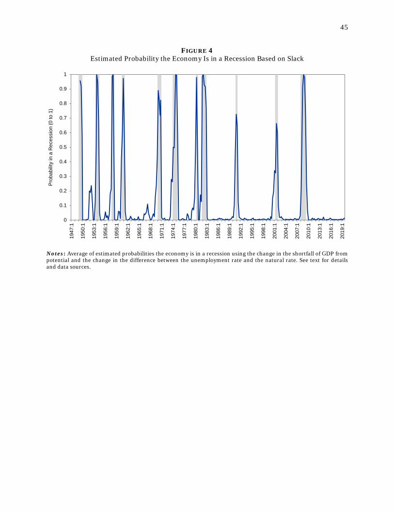
45

FIGURE 4 Estimated Probability the Economy Is in a Recession Based on Slack

Notes: Average of estimated probabilities the economy is in a recession using the change in the shortfall of GDP from potential and the change in the difference between the unemployment rate and the natural rate. See text for details and data sources.

0

0.1

0.2

0.3

0.4

0.5

0.6

0.7

0.8

0.9

1 1

947:

1

195

0:1

195

3:1

195

6:1

195

9:1

196

2:1

196

5:1

196

8:1

197

1:1

197

4:1

197

7:1

198

0:1

198

3:1

198

6:1

198

9:1

199

2:1

199

5:1

199

8:1

200

1:1

200

4:1

200

7:1

201

0:1

201

3:1

201

6:1

201

9:1

Pro

babi

lity

in a

Rec

essi

on (0

to 1

)

46

FIGURE 5 Estimated Probability the Economy Is in a Recession, 1929–1946

Notes: Average of estimated probabilities the economy is in a recession using the growth rate of industrial production, the growth rate of manufacturing employment, and the change in the unemployment rate. See text for details and data sources.

0

0.1

0.2

0.3

0.4

0.5

0.6

0.7

0.8

0.9

1 1

929:

1

193

0:1

193

1:1

193

2:1

193

3:1

193

4:1

193

5:1

193

6:1

193

7:1

193

8:1

193

9:1

194

0:1

194

1:1

194

2:1

194

3:1

194

4:1

194

5:1

194

6:1

Pro

babi

lity

in a

Rec

essi

on (0

to 1

)

47

TABLE 1 Economic Performance in Selected Postwar Episodes

Change in

Agreement Shortfall, Unemp. Shortfall, Employ. Employ. Avg. NBER of 2-Regime GDP from minus GDI from (Establ. (Househ. Weekly Quarter Rec.? Model Potential Nat. Rate Potential Survey) Survey) Hours 2007Q4 No 97% −0.6% 0.6% 2.3% 0.7% 0.9% −0.4% 2008Q1 Yes 21 4.2 0.9 1.7 0.2 1.5a −0.8 2008Q2 Yes 43 −0.2 1.4 2.7 −1.4 −0.8 −0.4 2008Q3 Yes 91 3.9 2.7 3.4 −2.1 −1.8 −0.8 2001Q1 No 66 4.8 1.4 −1.0 0.6 1.1 −0.8 2001Q2 Yes 32 1.1 0.7 4.0 −1.1 −1.9 −1.2 2001Q3 Yes 66 5.0 1.8 5.2 −1.2 −1.1 −1.2 1973Q4 No 74 −0.4 −0.2 −0.8 3.8 4.2 −0.7 1974Q1 Yes 50 7.0 1.4 6.7 1.9 2.2 −1.8 1974Q2 Yes 50 2.7 0.2 5.2 1.5 0.6 −1.1 1974Q3 Yes 87 7.5 1.7 5.8 0.6 1.1 −0.4 1990Q2 No 89 1.4 0.2 0.6 1.3 −0.4 −0.8 1990Q3 No 53 2.5 1.5 3.1 −0.5 −1.0 −1.2 1990Q4 Yes 72 6.4 1.8 4.6 −1.5 −1.2 −0.8 Notes: The two shortfall measures and the unemployment measure are in terms of percentage points per year. The final three measures are in terms of percent change at an annual rate. See text for details and data sources. a Adjusted for the discontinuity in the population measure used by the Bureau of Labor Statistics from December 2007 to January 2008, which reduced the reported change in employment by 598,000. See https://www.bls.gov/news.release/archives/empsit_02012008.pdf.

48

TABLE 2 Economic Performance in Selected Episodes in the 1930s

Change in

NBER Agreement of Industrial Manufacturing Unemployment Quarter Recession? 2-Regime Model Production Employment Rate 1932Q3 Yes 80% −9.2% −13.1% 9.8% 1932Q4 Yes 14 30.6 18.1 0.4 1933Q1 Yes 15 −19.5 −16.8 −2.1 1933Q2 No 99 74.4 24.6 4.0 1937Q2 No 95 7.0 12.6 −1.7 1937Q3 Yes 30 −6.5 3.3 −1.1 1937Q4 Yes 99 −79.2 −26.4 10.7 1934Q2 No 98 20.6 24.7 −3.0 1934Q3 No 44 −41.5 −12.8 12.4 1934Q4 No 78 11.3 −1.9 3.8 Notes: The industrial production and manufacturing employment measures are percent changes at an annual rate. The unemployment measure is percentage points per year. See text for details and data sources.

49

REFERENCES

Abramovitz, Moses. 1950. Inventories and Business Cycles. Studies in Business Cycles, No. 4. New York: National Bureau of Economic Research.

Burns, Arthur F., and Wesley C. Mitchell. 1946. Measuring Business Cycles. Studies in Business Cycles, No. 2. New York: National Bureau of Economic Research.

Business Cycle Developments (later Business Conditions Digest). Various issues. Washington, D.C.: U.S. Bureau of the Census.

Chauvet, Marcelle, and James D. Hamilton. 2006. “Dating Business Cycle Turning Points.” In Nonlinear Time Series Analysis of Business Cycles, edited by Costas Milas, Philip Rothman, and Dick van Dijk, 1–54. Amsterdam: Elsevier.

Davis, Joseph H. 2004. “A Quantity-Based Annual Index of U.S. Industrial Production, 1790–1915.” Quarterly Journal of Economics 119 (November): 1177–1215.

Davis, Joseph H. 2006. “An Improved Annual Chronology of U.S. Business Cycles since the 1790s.” Journal of Economic History 66 (March): 103–121.

Fabricant, Solomon. 1972. “The ‘Recession’ of 1969–1970.” In Economic Research: Retrospect and Prospect, Volume I, The Business Cycle Today, edited by Victor Zarnowitz. New York: NBER, pp. 89–136.

Friedman, Milton, and Anna Jacobson Schwartz. 1963. A Monetary History of the United States, 1867–1960. Studies in Business Cycles, No. 12. Princeton: Princeton University Press for NBER.

Hamilton, James D. 1989. “A New Approach to the Economic Analysis of Nonstationary Time Series and the Business Cycle.” Econometrica 57 (March): 357–384.

Hamilton, James D. 2011. “Calling Recessions in Real Time.” International Journal of Forecasting 27 (October–December): 1006–1026.

Hultgren, Thor, assisted by Maude R. Pech. 1965. Costs, Prices, and Profits: Their Cyclical Relations. Studies in Business Cycles, No. 14. New York: Columbia University Press for NBER.

Koopmans, Tjalling C. 1947. “Measurement without Theory.” Review of Economics and Statistics 29 (August): 161–172.

Kuznets, Simon. 1937. National Income and Capital Formation, 1919–1935. New York: National Bureau of Economic Research.

Kuznets, Simon, assisted by Lillian Epstein and Elizabeth Jenks. 1941. National Income and Its Composition, 1919–1938. New York: National Bureau of Economic Research.

Mintz, Ilse. 1969. Dating Postwar Business Cycles: Methods and Their Application to Western Germany, 1950-67. New York: Columbia University Press for NBER.

50

Mintz, Ilse. 1974. “Dating United States Growth Cycles.” Explorations in Economic Research 1 (Summer): 1–113.

Miron, Jeffrey A., and Christina D. Romer. 1990. “A New Monthly Index of Industrial Production, 1884–1940.” Journal of Economic History 50 (June): 321–337.

Mitchell, Wesley Clair. 1913. Business Cycles. Berkeley: University of California Press.

Mitchell, Wesley Clair. 1927. Business Cycles: The Problem and Its Setting. Studies in Business Cycles, No. 1. New York: National Bureau of Economic Research.

Mitchell, Wesley Clair. 1929. “A Review.” In Recent Economic Changes in the United States, produced by the Committee on Recent Economic Changes of the President's Conference on Unemployment. New York: McGraw-Hill Book Company, Inc. for NBER, 845–914.

Mitchell, Wesley Clair. 1951. What Happens during Business Cycles: A Progress Report. Studies in Business Cycles, No. 5. New York: National Bureau of Economic Research.

Mitchell, Wesley C., and Arthur F. Burns. 1936. “Production during the American Business Cycle of 1927–1933.” National Bureau of Economic Research Bulletin No. 61 (November 9): 1–20.

Mitchell, Wesley C., and Arthur F. Burns. 1938. “Statistical Indicators of Cyclical Revivals.” National Bureau of Economic Research Bulletin No. 69 (May 28): 1–12.

Moore, Geoffrey H. 1950. Statistical Indicators of Cyclical Revivals and Recessions. Occasional Paper 31, New York, National Bureau of Economic Research.

Moore, Geoffrey H. 1961a. “Appendix A: A Chronology of Business Cycles in the United States and Measures of Their Duration.” In Business Cycle Indicators, Volume I, edited by Geoffrey H. Moore. Studies in Business Cycles, No. 10. Princeton: Princeton University Press for NBER, 669–671.

Moore, Geoffrey H. 1961b. “Leading and Confirming Indicators of General Business Changes.” In Business Cycle Indicators, Volume I, edited by Geoffrey H. Moore. Princeton: Princeton University Press for NBER, 45–109.

Moore, Geoffrey H. 1961c. “Appendix B: Leads and Lags of Cyclical Indicators.” In Business Cycle Indicators, Volume I, edited by Geoffrey H. Moore. Studies in Business Cycles, No. 10. Princeton: Princeton University Press for NBER, 672–686.

Moore, Geoffrey H. 1975. “Slowdowns, Recessions, and Inflation: Some Issues and Answers.” Explorations in Economic Research 2 (Spring): 1–42.

Moore, Geoffrey H., and Julius Shiskin. 1967. Indicators of Business Expansions and Contractions. National Bureau of Economic Research Occasional Paper No. 103. New York: Distributed by Columbia University Press for NBER.

Moore, Geoffrey H., and Victor Zarnowitz. 1986. “Appendix A: The Development and Role of the National Bureau of Economic Research’s Business Cycle Chronologies.” In The American Business Cycle: Continuity and Change, edited by Robert J. Gordon. Studies in Business Cycles, No. 25. Chicago: University of Chicago Press for NBER, 735–780.

51

Persons, Warren M. 1926. “Theories of Business Fluctuations.” Quarterly Journal of Economics 41 (November): 94–128.

Romer, Christina D. 1994. “Remeasuring Business Cycles.” Journal of Economic History 54 (September): 573–609.

“Testing Business Cycles.” 1929. News-Bulletin of the National Bureau of Economic Research (March 1): 1–8.

Thorp, Willard Long. 1926. Business Annals. New York: National Bureau of Economic Research.

Watson, Mark W. 1994. “Business-Cycle Durations and Postwar Stabilization of the U.S. Economy.” American Economic Review 84 (March): 24–46.

Zarnowitz, Victor, and Charlotte Boschan. 1975. “Cyclical Indicators: An Evaluation and New Leading Indexes.” Business Conditions Digest (May): v–xiv.

Zarnowitz, Victor, and Geoffrey H. Moore. 1977. “The Recession and Recovery of 1973–1976.” Explorations in Economic Research 4 (Fall): 471–557.

Zarnowitz, Victor, and Geoffrey H. Moore. 1981. “The Timing and the Severity of the Recession of 1980.” NBER Reporter (Spring): 19–21.