nber - macro economic impact of brazil's alternative energy program
TRANSCRIPT
NBER WORKING PAPER SERIES
IS SUGAR SWEETER AT THE PUMP? THE MACROECONOMIC IMPACT OFBRAZIL’S ALTERNATIVE ENERGY PROGRAM
Marc D. WeidenmierJoseph H. Davis
Roger Aliaga-Diaz
Working Paper 14362http://www.nber.org/papers/w14362
NATIONAL BUREAU OF ECONOMIC RESEARCH1050 Massachusetts Avenue
Cambridge, MA 02138September 2008
The authors would like to thank Arevik Avedian, Clement Ogbomo and Lindsay Fay for excellentresearch assistance. The views expressed in this paper do not necessarily reflect the opinions of TheVanguard Group, nor those of the National Bureau of Economic Research.
© 2008 by Marc D. Weidenmier, Joseph H. Davis, and Roger Aliaga-Diaz. All rights reserved. Shortsections of text, not to exceed two paragraphs, may be quoted without explicit permission providedthat full credit, including © notice, is given to the source.

Is Sugar Sweeter at the Pump? The Macroeconomic Impact of Brazil’s Alternative EnergyProgramMarc D. Weidenmier, Joseph H. Davis, and Roger Aliaga-DiazNBER Working Paper No. 14362September 2008JEL No. E3,N1
ABSTRACT
The recent world energy crisis raises serious questions about the extent to which the United Statesshould increase domestic oil production and develop alternative sources of energy. We examine theenergy developments in Brazil as an important experiment. Brazil has reduced its share of importedoil more than any other major economy in the world in the last 30 years, from 70 percent in the 1970sto only 10 percent today. Brazil has largely achieved this goal by: (1) increasing domestic oil productionand (2) developing one of the world’s largest and most competitive sources of renewable energy --sugarcane ethanol -- that now accounts for 50 percent of Brazil's total gasoline consumption. A counterfactualanalysis of economic growth in Brazil from 1980-2008 suggests that GDP is almost 35 percent highertoday because of increased domestic oil production and the development of sugarcane ethanol. Wealso find a notable reduction in business-cycle volatility as a result of Brazil's progression to a morediversified energy program. Nearly three-fourths of the welfare benefits have come from domesticoil drilling, however, as rents have been paid to domestic factors of production during a time of risingoil prices. We discuss the potential implications of Brazil's energy program for the U.S. economy byconducting historical counterfactual exercises on U.S. real GDP growth since the 1970s.
Marc D. WeidenmierDepartment of EconomicsClaremont McKenna CollegeClaremont, CA 91711and [email protected]
Joseph H. DavisThe Vanguard GroupP.O. Box 2600, MS V37Valley Forge, PA 19482-2600and [email protected]
Roger Aliaga-DiazThe Vanguard GroupP.O. Box 2600, MS V37Valley Forge, PA [email protected]
The recent global energy crisis raises many questions about the extent to which the
United States should increase domestic oil and fossil fuel production as well as develop
alternative renewable sources of energy such as biofuels, wind, and solar power. Proponents of
drilling and fossil fuel production argue that existing technology has not advanced to the point
where alternative sources of energy can significantly reduce American dependence on fossil
fuels. Supporters of increased domestic oil production will also point out that rents largely go to
domestic factors of production as opposed to foreign countries. Critics of domestic oil production
argue that fossil fuels are destroying the environment and play a key role in global warming by
increasing the amount of carbon in the atmosphere (see DiPeso, 2003, Pickens, 2008; Johnson,
2008).
As shown by the current Presidential Election, one of the major challenges for American
policymakers is to develop a sensible energy policy that weighs the costs and benefits of
increased domestic oil production against cleaner, renewable alternative energy sources. This is a
difficult economic question for two reasons. First, there is little empirical evidence on the effects
of significantly reducing the share of imported oil on economic growth. As shown in Table 1, the
lack of empirical evidence on this question can probably be attributed to the fact that the share of
oil imported as a fraction of total oil consumption and production by the G7 economies has not
changed very much since the 1970s. Second, renewable energy sources account for about
approximately one percent of energy consumption in the G7 economies.
Fortunately, Brazil provides a historical experiment to examine the economic effects of
dramatically reducing a country’s share of imported oil as well as the impact of an important
alternative energy program. As shown in Figure 1, Brazil has reduced its share of imported oil
from about 70 to 10 percent over the last 30 years, more than any other major economy in the
1

world. The South American country has largely achieved this goal by increasing domestic oil
production and developing the world’s largest clean renewable alternative energy source that
competes directly with gasoline at the pump, sugarcane ethanol. Figure 2 shows that the clean
renewable alternative energy source currently accounts for over half of fuel demand in Brazil and
more than 23 percent of Brazil’s combined consumption of fossil and ethanol fuel (IPEA,
various issues).
We examine the effects of Brazil’s energy policies on its economic growth since 1980 by
extending models developed by Hamilton (1996, 2003) and Killian (2008a, 2008b, 2008c) to
include a country’s share of oil imports as a fraction of total oil consumption and production.
The empirical analysis suggests that real GDP is approximately 35 percent higher in Brazil
because the country has reduced its share of imported oil by increasing domestic oil production
and developing sugarcane ethanol so that rents go to domestic factors of production. We also
find a reduction in business-cycle volatility in the range of 14-22 percent as a result of Brazil’s
energy policies, with the most significant reductions coming over the past decade. We find that
approximately three-fourths of the welfare benefits are a direct result of increasing domestic oil
production during a period when oil prices have risen sharply.1
Brazil’s energy programs raise important questions about the extent to which the United
States should increase domestic oil production and develop alternative sources of energy. Since
alternative energy sources in the U.S. account at the present time for only a small percentage of
total energy consumption, we cannot specifically address this policy question. However, we can
examine the hypothetical historical impact to the U.S. economy had the United States
aggressively drilled all of the nation’s oil and natural gas reserves. What would have been the
1 Sugarcane ethanol is much cleaner than gasoline and has significant environmental benefits. We focus on the effects of Brazil’s sugarcane policy on economic growth and leave an analysis of the environmental impact for future research.
2

economic benefits? Would they have been sufficient to offset the negative effects of oil shocks
on U.S. economic activity? Would they have been sufficient to (at least temporarily) have made
the country “energy independent?”
To consider this possibility, we simulate U.S. economic growth over the last 30 years
under the (admittedly controversial) assumption that oil companies were allowed to drill in
ANWR and the public lands. A recent Bureau of Land Management Report to Congress (2008)
estimates that opening up the public lands to oil and natural gas production could yield as much
as 77 billion barrels of oil (and oil-barrel equivalents). We find that eliminating drilling
restrictions on the public lands would have raised US GDP by approximately 11 percent, or 1.5
trillion dollars in 2005(USD), over the last 33 years. However, we interpret these economic
benefits as an “upper bound” estimate since the counterfactual exercise assumes that the nation’s
improvements in energy intensity (oil consumed per unit of real GDP) was unaffected by this
radical change in domestic oil production. Under an alternative (and admittedly strong)
assumption that the nation’s energy intensity in 1977 would have remained constant through
2008, then the increases in domestic fossil fuel production would have yielded a more modest
cumulative increase of approximately seven to eight percent in the level of U.S. real GDP by the
first quarter of 2008.
Although our counterfactual results suggest that increased domestic fossil fuel production
could potentially have large economic benefits for the United States in the next 20 to 30 years,
the exercise also clearly demonstrates that the United States can not permanently drill its way to
“energy independence.” Alternative sources of energy (whether they be nuclear, wind, solar, or
bio-fuels) will eventually be needed so that the United States can more effectively reduce the
economy’s exposure to the negative effects of imported oil shocks.
3

We begin the analysis with a brief history of Brazil’s oil and sugarcane ethanol policies.
This is followed by an empirical analysis of oil and ethanol shocks on Brazilian economic
growth controlling for the percent of oil imported from foreign countries. Then we discuss the
implications of the Brazilian experience for the United States. This is followed by a
counterfactual analysis of US economic growth under the assumption that the public lands were
opened for drilling by the US government in the late 1970s. We conclude with a discussion of
the implication of the results for the U.S. economy.
II. A Brief History of Brazil’s Energy Policy, 1975-2008 A. Sugarcane Ethanol Program
The Brazilian economy experienced rapid economic growth in the late 1960s and early
1970s until the onset of the oil supply shocks. The 1973 oil shocks created two economic
problems for Brazil: (1) the cost of its oil imports—which constituted almost 80 percent of
domestic oil consumption—tripled in late 1973 because of the Arab oil embargo and (2) world
sugar prices declined sharply in 1974. The 1973 oil shock produced a large recession in Brazil
As a result, President Geisel launched the Programa Nacional do Álcool (National Alcohol
Program) or Pró-Álcool November 14, 1975. The program was designed to increase the
production of alcohol from sugar cane, modernizing and expanding existing distilleries, and
developing new production units. The program was intended to take advantage of the country’s
comparative advantage in producing sugarcane because of its tropical climate (Renato, 2007).
Pró-Álcool provided tax incentives to expand the sugar industry and was backed by
public and private sector investments. The Brazilian government launched a marketing program
4

with the slogan “Let’s unite, make alcohol.” Brazil required Petrobras, the country’s semi-public
oil monopoly to purchase and distribute sugarcane ethanol. The government offered low-interest
loans and credit guarantees for the construction of new refineries and taxed gasoline at a higher
rate at the pump. The government also mandated that transportation fuel be blended with a
minimum of 22 percent ethanol (Schmitz et al., 2007).
The results were dramatic. Between 1975 and 1979, ethanol production increased more
than 500 percent. The second stage of the program was launched in 1979, when the Brazilian
government signed agreements with major car companies to produce vehicles that ran on 100
percent ethanol. Fiat, Volkswagen, Mercedes-Benz, General Motors and Toyota agreed to
produce 250,000 ethanol-only cars in 1980 and 350,000 in 1982. The government program even
subsidized taxi drivers to purchase ethanol-only cars (Lashinsky and Schwartz, 2006).
During the early 1980’s, Brazil’s ethanol program flourished with high oil prices,
government intervention, and a World Bank loan that covered a portion of the costs. Between
1979 and 1985, ethanol production more than tripled in Brazil. The alternative fuel program
began to experience serious problems in the mid-1980s, however, as oil prices began to fall and
sugar prices started to rise. Nevertheless, automakers in Brazil continued to manufacture ethanol-
only cars in increasing amounts given the incentive system provided by the government. By the
late 1980’s, almost all new cars in Brazil were running on ethanol which produced a shortage of
the alternative fuel. Ironically, Brazil was forced to import ethanol and turn to a methanol blends
to keep ethanol-only cars on the road (Renato, 2007).
Political support for Pró-Álcool began to wane as oil prices declined in real and nominal
terms in the late 1980s and early 1990s. Ethanol production became less attractive which forced
the government to subsidize the producers via Petrobras. The government cut soft loans for the
5
construction of new ethanol refineries, and support for the ethanol program from state trading
companies was reduced and ultimately eliminated. Brazilian auto manufacturers retooled and
began to build gasoline cars again. By the mid-1990’s, the government only required fleet
vehicles (such as taxis and rental cars) to run on ethanol.
The Brazilian government made several changes to its sugarcane ethanol program in
1998. Petrobras’ monopoly over the distribution of ethanol was eliminated and ethanol prices
were no longer controlled by the government. Subsidies to the ethanol sector were largely
eliminated although the government continues to tax ethanol at a much lower rate at the pump.
Brazilian also regulates the percentage of ethanol in gasoline. Brazil increased the alcohol
content of gasoline from 20 to 22 percent in May 2001 and to 24 percent in June 2002. The
energy authorities apparently raise (lower) the blending rate when oil prices are high (low) and
sugar prices are relatively low (high) (Schmitz et al., 2007).
The introduction of new technologies in the last several years appears to be making
sugarcane ethanol a more viable alternative energy source. Ford introduced flex-fuel cars in
2002, followed by Volkswagen in 2003. Flex-fuel cars can operate on ethanol, gasoline or any
blend of the two fuels. The government creates incentives for consumers to purchase flex-fuel
cars by offering buyers a two percent lower sales tax compared to automobiles that run on
gasoline. In 2004, production of the flex-fuel cars increased to 328,300 and reached 5 million by
March of 2008. Approximately 90 percent of all new cars produced in Brazil are flex-fuel
(Associação Nacional dos Fabricantes de Veículos Automotores, 2007, 2008). This trend will
probably continue unless oil prices significantly decline in the coming years.
6
B. Domestic Oil Policy
Brazil recognized that ethanol could not solve the country’s energy problems. To boost
domestic oil production and reduce fossil fuel demand, the Brazilian government kept oil prices
artificially high in the 1980s to help fund oil exploration and drilling by Petrobras, the country’s
semi-public oil monopoly. Between 1980 and 2005, Brazil increased domestic crude oil
production on average of more than nine percent a year from, to 1.6 million barrels of oil per
day.
In the last couple of years, Petrobras has discovered huge oil deposits off the coasts of
Rio de Janiero and Sao Paolo that could increase the country’s oil reserves by more than 40
billion barrels.2 The government has also recently eliminated Petrobas’ oil monopoly in Brazil,
forcing the company to compete in the global marketplace. Reducing its dependence on oil
imports has long been a political priority in Brazil, where oil dependence was as high as 85
percent of its energy consumption in 1979 and plummeted to about 10 percent in 2002.3 Many
analysts believe that increased production and new oil discoveries have played the most
important role in reducing the country’s oil import share because rents go to domestic factors of
production rather than abroad, especially when oil prices are high.4 We now turn to the empirical
analysis to test the effects of the two energy programs on Brazilian economic growth over the
last 30 years.
2 BBC news http://news.bbc.co.uk/2/hi/business/7348111.stm. 3 EIA, 2008. 4 http://www.brazzilmag.com/content/view/9232/
7

III. Empirical Analysis
To analyze the economic effects of Brazil’s energy policies, we initially employ models
developed by Hamilton (1996, 2003).5 The general form of the model can be written as:
∑ ∑= =
−− +++=L
i
L
ititiitit oyy
1 1εγβα (1)
where yt is real GDP growth (or any measure of economic activity) in quarter t, reported at a
quarterly rate and ot is an oil price shock. Endogeneity is a potential problem in Equation (1) as
real GDP growth may cause changes in oil prices and changes in oil prices may cause real GDP
growth. Hamilton (1996) proposed a solution to solve the endogeneity problem by transforming
the oil price series to identify large oil shocks that can be attributed to well-known exogenous
such as geopolitical developments (in the Middle-East) that disrupt the world oil supply.
Hamilton suggests that oil shocks should be calculated as the percentage change in prices relative
to the price peak reached during the last year (if the shock is negative, then it is set to zero):6
))]...,,,(log()log(,0[ 1221 −−−−= ttttt popopoMAXpoMAXo (2)
where pot is oil prices, here measured by real West Texas Intermediate prices in US Dollars and
deflated by US CPI.
5 For an analysis of the effects of oil shocks on economic activity using Granger-causality tests and linear regressions, see Hamilton (1983, 1985, 1996, 2003), Mort (1989). Hooker (1996) argues that there is a structural break in the effect of oil price changes on the macroeconomy. For a discussion of oil shocks and monetary policy, see Bernanke (2004) and Bernanke et. al (1997). Hooker (2002) analyzes the inflationary effects of oil shocks. 6 Hamilton (2003) shows that the spikes in the transformed series coincide indeed with geopolitical events known to have resulted in disruptions in the world supply of oil.
8

In Brazil, where alternative energy sources are widely used, energy-cost shocks are
driven not only by changes in prices of each source (oil or ethanol) but also by the incidence of
each energy source in the total cost of energy bore by the consumers. To account for both
sources of energy, we modify Hamilton’s definition of an energy shock to include ethanol, te
))]...,,,(log()log(,0[ 1221 −−−−= ttttt pepepeMAXpeMAXe (3)
where pet is ethanol prices.
Annual ethanol prices are interpolated into higher frequency data using monthly sugar
cane prices (the key input into ethanol production). Sugar cane prices are compiled by Fundacion
Getulio-Vargas (FGV) and made available through Brazil’s IPEA database. The final quarterly
ethanol price series is deflated by Brazil’s GDP deflator. To account for oil and ethanol’s
fraction of total energy use, we combine the two individual oil and ethanol price shocks into a
single energy shock variable:
ttttt wewos ×+−×= )1( (4)
where is ethanol’s share of Brazil’s total consumption of ethanol and oil-derived products in
barrels. In our regressions, we also include a dummy variable (Dt) to account for Brazil’s
macroeconomic stabilization program following the country’s high-inflation and hyperinflation
in the late 1980s and early 1990s.
tw
7
The model can now be written as:
(5) ∑ ∑= =
−− ++++=L
itti
L
iitiitit Dsyy
1 1εδγβα
7 We set the dummy variable to 1 if annual inflation rate is below 15%. This dummy takes value 1 for most of the period post-July 1994, the year in which Brazil successfully implemented the stabilization program known as “Plan Real”. We also tested to see if there was a structural break at this known date. Using a Chow test, we were unable to reject the null hypothesis of no structural break.
9

Quarterly GDP data for Brazil are taken from the official statistics of the South American
country, IPEA.8 The sample covers the period January 1980-2008.9 The results for the baseline
Hamilton specification are reported in Column 1 of Table 2. The F-statistics shows that oil
shocks in Brazil do not have a statistically significant effect on economic activity in the South
American country.
One problem with the baseline regression is that the analysis does not control for the
large change in Brazil’s oil import share over time. This might explain why oil shocks do not
have a statistically significant effect on Brazil’s real GDP growth. To consider this possibility,
we weight the energy shocks by the percent of oil and ethanol imported into Brazil. The
“normalized” net import coefficient for oil and ethanol is defined as = (consumption –
production) / (consumption + production) and ∈ [-1, 1]. If the normalized net import
coefficient took a value of one, this would indicate that all oil/ethanol consumed is being
imported and there is no domestic production. As shown in Figure 1, Brazil has drastically
reduced its dependency on foreign oil in the period 1975-2008. In order to account for the
changing degree of foreign oil dependence in our energy shock variable we modify (4) as
follows:
ethanoloiltm ,
ethanoloiltm ,
ettt
ottt
mt mwemwos ××+×−×= )1( (6)
We then re-estimate model (5) with stm substituted for st. The results are reported in Column 2 of
Table 1. Peak oil shocks, adjusted for the percent of oil imported, are now jointly significant at
8 www.ipea.gov.br9 We would like to include the 1970s in the analysis since the historical record suggests that oil shocks had a particularly large negative effect on Brazil. Unfortunately, quarterly GDP data, quarterly ethanol consumption and quarterly ethanol production data for Brazil are not available for the 1970s. If the 1970s oil shocks had large negative effects on Brazil, then our results would provide a lower bound estimate on the gains from domestic energy production in the South American country.
10
the 3 percent level. This suggests that reducing the oil import share has reduced the negative
effects of oil shocks. Rents paid to domestic factors of energy production offset the effects of
peak oil on economic activity. Indeed, as shown in Figure 3, the effect of oil shocks on real GDP
growth in Brazil has fallen by approximately 80 percent since 1980, from .1 to .02 percent.
Finally, we define a third type of energy shock that controls for energy intensity. We
multiply our energy shock variable by a measure of energy intensity that is defined as total
barrels of oil and ethanol combined per unit of real GDP (ethanol consumption was converted to
oil-equivalent quantities based on ethanol BTU equivalence to oil).10 If we define as it the energy
intensity coefficient, our specification (5) becomes:
∑ ∑= =
−−− ++++=L
itti
L
iit
mitiitit Disyy
1 1εδγβα (5’)
As shown in Column 3 of Table 2, the energy shocks weighted by intensity are jointly
significant at the 2 percent level. The magnitude of the energy shocks is approximately the same
size as the energy shocks reported in Column 2 of Table 2.
The basic idea behind equations (1)-(5’) is to estimate the response of economic activity
to exogenous changes in the prices of oil and ethanol. Kilian (2008a, 2008b, forthcoming) argues
that Hamilton’s (1996) non-linear transformation of oil price shocks defined in equation (2) does
not adequately identify supply and demand shocks.11 Oil price shocks respond primarily to
precautionary demand shocks rather than to supply shocks. Precautionary demand price changes
are triggered by commercial users of oil who want to hedge against the possibility of an oil
10 Ethanol’s energy content is 76330 BTU/gal or 3205859.919 BTU/bbl of ethanol (1bbl = 42 gal). For gasoline, 116090 BTU/gal. Since 19.2 gal of gasoline can be refined from 1 bbl of oil; so 116090*19.2 = 2228928 BTU/bbl of oil. So the conversion coefficient is approximately 1.44 bbl of oil per bbl of ethanol (3205859.919 / 2228928). 11 Endogeneity bias would lead to inconsistent estimation of the parameters in [1]-[3]. Suppose that oil and ethanol prices are driven by demand and supply shocks in oil and ethanol markets, respectively. Suppose further, that these supply and demand shocks impact Brazil GDP both directly and indirectly via oil and ethanol prices (see Kilian, forthcoming). Then, the residuals would then be correlated with the oil or ethanol price shocks, violating a key assumption for OLS.
11
shortage in the future (and by speculators in search of a profit under the belief that oil will be
relatively scarce in the future). Therefore, Killian argues that it is necessary to disentangle
precautionary demand from ordinary current crude oil demand.
We adopt Kilian’s (forthcoming) three-variable structural (SVAR) specification to separately
identify oil supply and demand shocks, with the exception that we apply Hamilton’s transformation after
removing global demand shocks from the analysis to identify peak oil shocks. The three-variable system
includes the percentage change in oil production, a de-trended global economic activity indicator, and
the percentage changes in real oil prices. For the global economic activity indicator, we use the Baltic
Exchange Dry Index from Datastream.12 World oil prices are proxied by West Texas Intermediate spot
prices deflated by the US consumer price index. Our sample period covers quarterly data from January
1975 to March 2008. We allow for twelve lags in the VAR specification to capture the dynamics in the
system.
Following Kilian (forthcoming) we impose two identifying restrictions to uncover the structural
shocks from the reduced form VAR. First, unanticipated oil-production shocks (i.e. the residuals of the
oil-production equation in the VAR) are driven by supply-side decisions. This means that oil producers
can not respond to higher oil prices (even if they wanted to) or to speculative trading by investors in a
period as short as a month. Second, unanticipated changes in global demand (i.e. the residuals of the
global demand equation in the VAR) are unlikely to be caused by unexpected oil prices changes taking
place within the same month. Global demand is also unlikely to be affected by speculation shocks either.
With these identifying restrictions, we can recursively identify oil supply and demand shocks using a
standard Choleski decomposition.
The model can be written as follows:
12 The Baltic index is available since May 1985. We extend the series back to January 1975 using OECD world industrial production index, from Datastream. Kilian (forthcoming) reports his results remain unaltered when using OECD world industrial production instead of his preferred global economic activity indicator.
12

⎥⎥⎥
⎦
⎤
⎢⎢⎢
⎣
⎡
×⎥⎥⎥
⎦
⎤
⎢⎢⎢
⎣
⎡=
⎥⎥⎥
⎦
⎤
⎢⎢⎢
⎣
⎡
demandprec
demandg
plyoil
priceoil
activityecon
production
aaaaa
a
_
.
sup_
333231
2221
11
_
. 000
ννν
εεε
(6)
The ε are the unexpected shocks (or the residuals) from the regular reduced-form three variable
VAR system and the ν’s are the unobserved structural shocks. The underlying structural shocks
can be identified using the recursive identification scheme. Figure A1, in the appendix, displays
the oil-price series resulting from the estimated SVAR, which excludes exogenous global
demand shocks.
Table 3 displays regression output for models (5) and (5’) but based on applying an
analogous to Hamilton’s transformation (equation 2) to this oil-price series (we label this model
“Kilian specification”, since it is based on Kilian’s SVAR identification of exogenous oil
shocks). The results reported in Table 3 are quite similar to the analysis using the standard
Hamilton’s transformation. Column 1 of Table 3 shows that an oil shock does not have a
statistically significant effect on economic growth. However, oil shocks reduce real GDP growth
in Brazil once we weight oil shocks by the oil import share and energy intensity. The weighted
energy shocks are statistically significant at the one percent level in Columns 2 and 3 of Table 3.
By increasing domestic production, Brazil has reduced the negative effects of oil shocks. As
shown in Figure 4B, the time-varying impact of oil shocks has also fallen around 80 percent for
Brazil in the Kilian specification, from .12 percent to almost .02 percent.
Counterfactual exercises for Brazil
Hamilton (2003) runs a regression similar to equation (1) for the United States using peak
oil shocks defined in equation (2). He then conducts simple counterfactual exercises based on
13

setting ot = 0. That is, what would have been U.S. GDP growth there had been no oil shocks
during the sample period? The difference between the counterfactual fitted values (with ot = 0)
and the true fitted values is a measure of the GDP growth gain the country would have
experienced there had been no oil shocks.
For Brazil, we believe that the appropriate counterfactual analysis is to assume no ethanol
program and no change in the net oil import share since the late 1970s. We perform the
counterfactual analysis using our Hamilton and Killian specifications. This counterfactual
scenario implies to set (and thus ) and . is the net import
coefficient, as of 1980:Q1, that arises from the total oil plus ethanol combined consumption
(based on ethanol’s BTU oil-equivalence). The difference between the counterfactual fitted
values and the true fitted values is a measure of the GDP growth loss Brazil would have
experienced under the proposed scenario of no ethanol program and neglecting the impact of
discoveries of oil. As shown in Figures 5A (Hamilton counterfactual) and 5B (Killian
counterfactual), Brazil’s energy program suggests that GDP would be approximately 30 and 35
percent lower in Brazil if the country did not reduce its share of imported oil by increasing
domestic energy production (oil and sugarcane ethanol) since 1980. The large welfare gains
suggest that increased domestic energy production (oil and sugarcane ethanol) has largely offset
the negative effects of oil shocks because rents are now paid to domestic factors (rather than
foreign factors).
0=tw ott
mt mos ×= eoo
t mm += 1980eom +
1980
We then run a second counterfactual scenario that keeps the assumption of no ethanol
program but it allows for new discoveries of oil during the sample period. That is, we now set
(and thus ) and . Thus, we let to change through time
according to Brazil’s increasing production of oil, but accounting for the extra oil consumption
0=tw ott
mt mos ×= eo
tot mm += eo
tm +
14

needed to make up for the lost ethanol production (again, based on ethanol’s BTU oil-
equivalence). The difference between counterfactual and actual fitted values in (5’) is the GDP
growth loss Brazil would have experienced without the Pro-Álcool program.
Finally, the difference between the two counterfactuals can be interpreted as the GDP loss
resulting only from new oil discoveries. The simulations show that approximately three-quarters
of the welfare gains actually experienced by Brazil (relative to the counterfactual scenario) can
be attributed to an increase in domestic oil discoveries rather than to Brazil’s sugarcane ethanol
program. Still, our results indicate that sugarcane ethanol has been successful in helping to
partially insulate Brazil’s economy from imported oil shocks.13 Under the counterfactual case of
no ethanol program, the level of Brazil’s real GDP would be approximately 8 percent lower.
In evaluating the macroeconomic and welfare effects of Brazil’s reduced foreign oil
dependence, it is also important to examine the potential business cycle effects of Brazil’s energy
policy. An example would include mitigating the impact of terms-of-trade shocks on output
volatility, as Brazil is a price-taker in world oil markets. Assuming reasonable levels of risk
aversion for Brazilian households, and to the extent that liquidity constraints and market
imperfections prevent households from perfectly smoothing consumption, welfare would be
unambiguously increased if output volatility is lower.
Table 4 compares Brazil’s historical GDP growth volatility against output volatility under
the two counterfactual scenarios described before. Since 1980, Brazil has been able to reduce
average output volatility (as defined by the standard deviation in quarterly real GDP growth) by
approximately 14 to 22 percent. Since 1995, business-cycle volatility has been reduced by as
much as 33 percent using the Kilian derivation for exogenous oil-price shocks. 13 Sugarcane ethanol has also reduced air pollution in Brazil’s major cities. The environmental benefits of sugarcane ethanol are not considered in this paper. We leave this as an item for future research.
15

Counterfactual exercises for the United States
The success of Brazil energy program raises important questions about the economic
effects of reducing the oil import share in the United States by increasing domestic production of
fossil fuels and developing alternative sources of energy. As shown in Figure 6, the oil import
share for the United States has risen from about 40 to 60 percent in the last 30 years. The rise in
the share of oil imports has been partially offset by a decrease in energy intensity, however. Most
experts predict that the US will import approximately 70 percent of its oil over the next 30 years
unless there is a significant change in US energy policy (EIA, 2004).
To examine the effects of oil shocks on economic activity in the United States, we
estimate Hamilton and Killian specifications using quarterly data from 1977 to 2008Q1.14 Tables
5 and 6 show that oil shocks have a negative and statistically significant on US GDP growth in
all three specifications. Contrary to Brazil, the regression coefficients on lagged oil-price shocks
do not change markedly when one controls for the level of the U.S. net import share and the level
of oil intensity. However, the U.S. may be a special case since net imports have been trending
higher while oil intensity has been falling, with the product of the two trends effectively yielding
a flat line.
From the regressions in Tables 5 and 6, we estimate a series of counterfactual to examine
the effects of reducing US imported oil share by increasing domestic production. The Bureau of
Land Management (2008) has recently published a report that estimates the amount of oil and
natural gas reserves –the equivalent of about 77 billion barrels of oil--in restricted areas such as
Federal lands. The BLM reports that oil and natural gas reserves from these restricted areas could
have reduced US oil import share to about 14 percent over the period 1975-2008Q1.
14 Model (5’) is still valid for the U.S., since in this case wt = 0 in the estimation sample. Kilian SVAR is also valid for the U.S. as it depends only on world-level variables: world oil production, global demand and world oil market prices.
16

The counterfactual assumes that the United States uses all of its oil and natural gas
reserves in the restricted areas during the period 1975-2008Q1. As shown in Figures 7a and 7b,
the cumulative effect of reducing the US net oil import share to 14 percent would have increased
GDP in the United States by about eleven percent, or 1.5 trillion dollars, over the last 33 years.
US GDP is seven or eight percent higher if we make the strong assumption that there has been no
change in energy intensity to accompany the increase in domestic energy production since the
late 1970s.
IV. Conclusion
Should the United States increase domestic oil production? Should the United States
develop alternative and renewable sources of energy? Although these questions have recently
received quite a bit of attention in the press and Presidential Election given the recent rise in oil
prices, there is little empirical evidence on the costs and benefits of these policies on economic
growth. The absence of empirical evidence on this question can probably be attributed to the fact
that G7 and OECD countries import a relatively constant share of oil and do not use alternative
fuels as a major source of energy. Given these facts, we use Brazil as an historical experiment.
Unlike any other major economy in the world, Brazil has reduced its share of imported oil from
70 to nearly 10 percent since the 1970s oil shocks. The South American country has reduced its
share of imported oil by: (1) increasing domestic oil production and (2) developing the world’s
largest clean, renewable alternative energy source that competes with gasoline at the pump,
sugarcane ethanol.
We test the economic effects of these two energy policies on Brazilian economic growth
extending models developed by Hamilton (1996) and Killian (2007) to include a country’s share
17

of imported oil. We find that the accrued macroeconomic benefits of Brazil’s energy policies
have been economically large and significant. Indeed, the empirical analysis suggests that
Brazil’s diversified energy policy has increased the country’s GDP by approximately 35 percent
(or, equivalently, $463 billion) since 1980. Without these changes in energy policies, Brazil’s
economy would rank 15th (behind Mexico) in terms of world GDP, rather than its current 2007
ranking of 10th. Notably, we find that three-quarters of the welfare benefits of the policy can be
attributed to an increase in domestic oil production during a period of rising oil prices. Still, our
results indicate that sugarcane ethanol has been successful in helping to partially insulate Brazil’s
economy from imported oil shocks.15 Under the counterfactual case of no ethanol program, the
level of Brazil’s real GDP would be approximately 8 percent lower today, and business-cycle
volatility would be approximately 2-5 percent higher.
Brazil’s energy programs raise important questions about the extent to which the United
States should increase domestic oil production and develop alternative sources of energy. Since
alternative energy sources in the U.S. account at the present time for only a small percentage of
total energy consumption, we cannot specifically address this policy question. However, we can
examine the hypothetical historical impact to the U.S. economy had the United States
aggressively drilled all of the nation’s oil and natural gas reserves. We simulate U.S. economic
growth under the (admittedly controversial) assumption that energy companies were allowed to
drill all of the oil and natural gas on the public lands between 1976 and 2008. Our analysis
suggests that eliminating drilling restrictions on the public lands would have raised US GDP by
approximately 11 percent, or 1.5 trillion dollars in 2005(USD), over the last 33 years. We
interpret these economic benefits as an “upper bound” estimate since the counterfactual exercise 15 Sugarcane ethanol has also reduced air pollution in Brazil’s major cities. The environmental benefits of sugarcane ethanol are not considered in this paper. We leave this as an item for future research.
18
assumes that the nation’s improvements in energy intensity (i.e., oil consumed per unit of real
GDP) was unaffected by this radical change in domestic oil production. We also find that US
GDP would be seven or eight percent higher by increasing domestic production if we assume
that energy efficiency has not changed since 1977.
Overall, our analysis suggests that increased domestic fossil fuel production could
potentially have large economic benefits for the United States in the next 20 to 30 years. The
results also suggest that the United States can not drill its way to energy independence.
Alternative sources of energy such as nuclear, wind, solar, or others as well as innovations in
fuel efficiency will eventually be needed so that the United States can more effectively reduce
the negative effects of imported oil shocks on economic activity.
19

References Associação Nacional dos Fabricantes de Veículos Automotores, Various reports. Bernanke, Ben S., 2004. “Oil and the Economy.” Speech delivered at the Distinguished Lecture Series, Darton College, Albany, GA, October 21. Available at http://www.federalreserve.gov/boarddocs/speeches/2004/20041021/default.htm Bernanke, Ben S., Gertler, Mark, and Mark Watson, 1997. “Systematic Monetary Policy and the Effects of Oil Price Shocks.” Brookings Papers on Economic Activity, pp. 91–142. DiPeso, Jim. 2003. “Foreign Oil Dependence Entangles US with Regimes that Finance Terror. Does Buying SUVS Promote Terrorism.” Detroit News, January 12. Energy Information Administration, 2004. Long Term Oil Supply Scenarios. Washington, D.C. Energy Information Administration, 2008. World Crude Oil Production. Hamilton, James D., 1983. “Oil and the Macroeconomy Since World War II.” Journal of Political Economy 91: 228-248. Hamilton, James D., 1985. “Historical Causes of Postwar Oil Shocks and Recessions.” Energy Journal 6: 97-116. Hamilton, James D., 1996. “This is What Happened to the Oil Price-Macroeconomy Relationship.” Journal of Monetary Economics 38(2): 215–20. Hamilton, James D., 2003. “What is an Oil Shock?” Journal of Econometrics 113: 363–98. Hooker, Mark A., 2002. “Are Oil Shocks Inflationary? Asymmetric and Nonlinear Specifications Versus Changes in Regime.” Journal of Money, Credit and Banking 34 (May): 540–61. Hooker, Mark A., 1996. “What Happened to the Oil-Price-Macroeconomy Relationship?” Journal of Monetary Economics 38: 195-213. Instituto de Pequisa Economica Aplicada. www.ipea.gov.br Inventory or Onshore Fedearl Oil and Natural Gas Resources and Restrictions to their Development. 2008. Washington: Bureau of Land Management, US Department of the Interior. Johnson, Keith 2008. “Drill Baby Drill, If it Makes Economic Sense, That Is.” Wall Street Journal Blog, September 9. Kilian, Lutz, 2008a. “Exogenous Oil Supply Shocks: How Big Are They and How Much Do They Matter for the U.S. Economy?” Review of Economics and Statistics 90:216-240.
20

Kilian, Lutz, 2008b. “A Comparison of the Effects of Exogenous Oil Supply Shocks on Output and Inflation in the G7 Countries.” Journal of the European Economic Association 6: 78-121. Kilian, Lutz, forthcoming. “Not All Oil Price Shocks Are Alike: Disentangling Demand and Supply Shocks in the Crude Oil Market.” American Economic Review. Lashinshky, Adam and Nelson Schwartz. (2006). “How to Beat the High Cost of Gasoline Forever!” Fortune. http://money.cnn.com/magazines/fortune/fortune_archive/2006/02/06/8367959/index.htm Mort, Knut A., 1989. “Oil and the Macroeconomy When Prices Go Up and Down: An Extension of Hamilton’s Results.” Journal of Political Economy 91: 740-744. Pickens, T. Boone. 2008. “This is My Plan for American Energy, What’s Yours?” Wall Street Journal, September 2, A22. Raymond, Jennie E. and Robert Rich, 1997. “Oil and the Macroeconomy: A Markov-State Switching Approach.” Journal of Money, Credit, and Banking 29: 193-213. Schmitz, Troy, Seale, James L., and Peter Buzzanell. 2007. “Brazil’s Domination of the World’s Sugar Market.” Arizona State University Working Paper.
21

Table 1. Net Oil Import Share for the World’s Ten Largest Economies:1980 vs. 2008 (in percent)
Country 1980 2008 Change(Percentage Points) Brazil 70 10 -60 Canada 13 -5 -18 France 98 98 0 Germany 93 95 2 Italy 96 88 -8 Japan 100 100 0 Spain 94 100 6 United Kingdom 3 10 7 United States 33 60 27 Source: IMF, EIA Notes: Russia is not included in the table because of data constraints.
22

Table 2. Hamilton Regressions for Brazil, 1980-2008Q1 Independent Variable Column 1 Column 2 Column 3 GDP Growth(-1) 0.073 0.138 0.138 (0.572) (0.284) (0.286) GDP Growth(-2) -0.076 -0.111 -0.115 (0.050) (0.238) (0.214) GDP Growth(-3) -0.191 -0.19 -0.187 (0.029) (0.036) (0.039) GDP Growth(-4) -0.052 -0.04 -0.041 (0.630) (0.744) (0.740) Energy Shock(-1) – st-1 -0.054 (0.255) Energy Shock(-2) – st-2 0.02 (0.455) Energy Shock(-3) – st-3 -0.001 (0.949) Energy Shock(-4) – st-4 -0.009 (0.599) Energy Shock weighted by Import Share(-1) – sm
t-1 -0.157 (0.129) Energy Shock weighted by Import Share(-2) – sm
t-2 0.113 (0.051) Energy Shock weighted by Import Share(-3) – sm
t-3 -0.042 (0.319) Energy Shock weighted by Import Share(-4) – sm
t-4 -0.063 (0.060) Energy Shock weighted by Import Share and Intensity(-1) – sm
t-1 it-1 -0.127 (0.142) Energy Shock weighted by Import Share and Intensity(-2) – sm
t-2 it-2 0.096 (0.045) Energy Shock weighted by Import Share and Intensity(-3) – sm
t-3 it-3 -0.036 (0.295) Energy Shock weighted by Import Share and Intensity(-4) – sm
t-4 it-4 -0.048 (0.085) Inflation dummy - Dt 0.005 0.004 0.004 (0.204) (0.306) (0.304) R-squared 0.09 0.136 0.134 P-value for F-Statistic of Energy Shocks (0.328) (0.028) (0.033) Observations 109 109 109 Note:p-values are in parenthesis
23

Table 3. Kilian Regressions for Brazil, 1980-2008 Independent Variable Column 1 Column 2 Column 3 GDP Growth(-1) 0.115 0.204 0.203 (0.350) (0.132) (0.136) GDP Growth(-2) -0.101 -0.156 -0.16 (0.353) (0.130) (0.114) GDP Growth(-3) -0.196 -0.194 -0.19 (0.028) (0.050) (0.054) GDP Growth(-4) -0.041 -0.016 -0.017 (0.708) (0.895) (0.889) Energy Shock(-1) – st-1 -0.092 (0.027) Energy Shock(-2) – st-2 0.044 (0.160) Energy Shock(-3) – st-3 0.002 (0.924) Energy Shock(-4) – st-4 -0.013 (0.462) Energy Shock weighted by Import Share(-1) – sm
t-1 -0.238 (0.006) Energy Shock weighted by Import Share(-2) – sm
t-2 0.182 (0.008) Energy Shock weighted by Import Share(-3) – sm
t-3 -0.047 (0.358) Energy Shock weighted by Import Share(-4) – sm
t-4 -0.081 (0.036) Energy Shock weighted by Import Share and Intensity(-1) – sm
t-1 it-1 -0.193 (0.008) Energy Shock weighted by Import Share and Intensity(-2) – sm
t-2 it-2 0.152 (0.008) Energy Shock weighted by Import Share and Intensity(-3) – sm
t-3 it-3 -0.04 (0.342) Energy Shock weighted by Import Share and Intensity(-4) – sm
t-4 it-4 -0.062 -0.058 Inflation dummy - Dt 0.005 0.003 0.003 (0.161) (0.357) (0.354) R-squared 0.135 0.188 0.184 P-value for F-Statistic of Energy Shocks 0.244 0.001 0.002 Observations 109 109 109 Note:p-values are in parenthesis
24

Table 4. Brazil real GDP growth summary statistics: Actual vs counterfactual * Data Hamilton Counterfactual Kilian Counterfactual 1981Q1 – 2008Q1 Scenario 1 Scenario 1 + 2 Scenario 1 Scenario 1 + 2 Mean 2.5% 2.2% 1.3% 2.2% 1.1% Std dev 7.9% 8.1% 9.2% 8.3% 10.1% CV 3.1 3.6 6.8 3.7 9.3 1995Q1 – 2008Q1 Mean 2.7% 2.3% 0.8% 2.2% 0.4% Std dev 4.8% 4.9% 6.0% 5.0% 7.2% CV 1.8 2.1 7.4 2.2 18.7
* Note: two counterfactual scenarios, Scenario 1: No Pro-Álcool Program (wt = 0) and increased oil consumption from substitution of BTU-equivalent quantities of ethanol with oil (mo
t = mo+et ).
Scenario 2: Increased net imports of oil from neglecting oil discoveries since 1980Q1 (mot = mo
80Q1 ).
25

Table 5. Hamilton Regressions for United States, 1975Q1-2008Q2 Independent Variable Column 1 Column 2 Column 3 GDP Growth(-1) 0.214 0.228 0.213 (0.010) (0.005) (0.012) GDP Growth(-2) 0.068 0.082 0.069 (0.525) (0.421) (0.518) GDP Growth(-3) 0.016 0.015 0.017 (0.865) (0.872) (0.860) GDP Growth(-4) -0.052 -0.045 -0.053 (0.660) (0.704) (0.656) Energy Shock(-1) – ot-1 -0.011 (0.217) Energy Shock(-2) – ot-2 -0.006 (0.330) Energy Shock(-3) – ot-3 -0.007 (0.615) Energy Shock(-4) – ot-4 -0.011 (0.003) Energy Shock weighted by Import Share(-1) – o t-1mt-1 -0.021 (0.349) Energy Shock weighted by Import Share(-2) – o t-2mt-2 -0.008 (0.553) Energy Shock weighted by Import Share(-3) – o t-3mt-3 -0.009 (0.728) Energy Shock weighted by Import Share(-4) – o t-4mt-4 -0.026 (0.076) Energy Shock weighted by Import Share and Intensity(-1) – o t-1 mt-1 it-1 -0.009 (0.258) Energy Shock weighted by Import Share and Intensity(-2) – o t-2 mt-2 it-2 -0.004 (0.435) Energy Shock weighted by Import Share and Intensity(-3) – o t-3 mt-3 it-3 -0.007 (0.565) Energy Shock weighted by Import Share and Intensity(-4) – o t-4 mt-4 it-4 -0.01 (0.004) Inflation dummy - Dt -0.007 -0.007 -0.008 (0.275) (0.274) (0.268) R-squared 0.17 0.151 0.17 P-value for F-Statistic of Energy Shocks (0.038) (0.047) (0.047) Observations 134 134 134 Note:p-values are in parenthesis
26

Table 6. Kilian Regressions for United States, 1975Q1-2008Q2 Independent Variable Column 1 Column 2 Column 3 GDP Growth(-1) 0.217 0.229 0.216 (0.009) (0.005) (0.011) GDP Growth(-2) 0.069 0.082 0.07 (0.513) (0.419) (0.508) GDP Growth(-3) 0.016 0.014 0.016 (0.871) (0.882) (0.870) GDP Growth(-4) -0.055 -0.048 -0.056 (0.643) (0.686) (0.638) Energy Shock(-1) – ot-1 -0.01 (0.249) Energy Shock(-2) – ot-2 -0.006 (0.387) Energy Shock(-3) – ot-3 -0.007 (0.635) Energy Shock(-4) – ot-4 -0.011 (0.000) Energy Shock weighted by Import Share(-1) – o t-1mt-1 -0.017 (0.424) Energy Shock weighted by Import Share(-2) – o t-2mt-2 -0.01 (0.535) Energy Shock weighted by Import Share(-3) – o t-3mt-3 -0.008 (0.788) Energy Shock weighted by Import Share(-4) – o t-4mt-4 -0.028 (0.034) Energy Shock weighted by Import Share and Intensity(-1) – o t-1 mt-1 it-1 -0.009 (0.282) Energy Shock weighted by Import Share and Intensity(-2) – o t-2 mt-2 it-2 -0.004 (0.500) Energy Shock weighted by Import Share and Intensity(-3) – o t-3 mt-3 it-3 -0.008 (0.599) Energy Shock weighted by Import Share and Intensity(-4) – o t-4 mt-4 it-4 -0.01 (0.000) Inflation dummy - Dt -0.007 -0.007 -0.008 (0.267) (0.266) (0.261) R-squared 0.168 0.151 0.168 P-value for F-Statistic of Energy Shocks (0.006) (0.008) (0.008) Observations 134 134 134 Note:p-values are in parenthesis
27
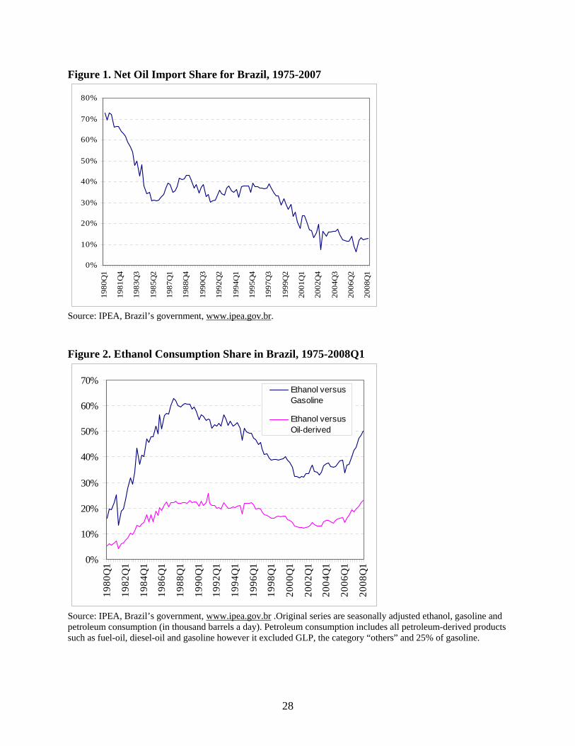
Figure 1. Net Oil Import Share for Brazil, 1975-2007
0%
10%
20%
30%
40%
50%
60%
70%
80%19
80Q
1
1981
Q4
1983
Q3
1985
Q2
1987
Q1
1988
Q4
1990
Q3
1992
Q2
1994
Q1
1995
Q4
1997
Q3
1999
Q2
2001
Q1
2002
Q4
2004
Q3
2006
Q2
2008
Q1
Source: IPEA, Brazil’s government, www.ipea.gov.br. Figure 2. Ethanol Consumption Share in Brazil, 1975-2008Q1
0%
10%
20%
30%
40%
50%
60%
70%
1980
Q1
1982
Q1
1984
Q1
1986
Q1
1988
Q1
1990
Q1
1992
Q1
1994
Q1
1996
Q1
1998
Q1
2000
Q1
2002
Q1
2004
Q1
2006
Q1
2008
Q1
Ethanol versusGasoline
Ethanol versusOil-derived
Source: IPEA, Brazil’s government, www.ipea.gov.br .Original series are seasonally adjusted ethanol, gasoline and petroleum consumption (in thousand barrels a day). Petroleum consumption includes all petroleum-derived products such as fuel-oil, diesel-oil and gasoline however it excluded GLP, the category “others” and 25% of gasoline.
28

Figure 3. Ethanol Exports for Brazil, 1980-2008Q1
-30%
-25%
-20%
-15%
-10%
-5%
0%
5%
10%
1980
Q1
1981
Q4
1983
Q3
1985
Q2
1987
Q1
1988
Q4
1990
Q3
1992
Q2
1994
Q1
1995
Q4
1997
Q3
1999
Q2
2001
Q1
2002
Q4
2004
Q3
2006
Q2
2008
Q1
Source: IPEA, Brazil’s government, www.ipea.gov.br.
29

Figure 4. Time-Varying Impact of Oil Shocks on Real GDP Growth in Brazil, 1980-2008* A. Hamilton Specification
-0.120
-0.100
-0.080
-0.060
-0.040
-0.020
0.00019
80Q
1
1981
Q3
1983
Q1
1984
Q3
1986
Q1
1987
Q3
1989
Q1
1990
Q3
1992
Q1
1993
Q3
1995
Q1
1996
Q3
1998
Q1
1999
Q3
2001
Q1
2002
Q3
2004
Q1
2005
Q3
2007
Q1
B. Killian Specification
-0.160
-0.140
-0.120
-0.100
-0.080
-0.060
-0.040
-0.020
0.000
1980
Q1
1981
Q3
1983
Q1
1984
Q3
1986
Q1
1987
Q3
1989
Q1
1990
Q3
1992
Q1
1993
Q3
1995
Q1
1996
Q3
1998
Q1
1999
Q3
2001
Q1
2002
Q3
2004
Q1
2005
Q3
2007
Q1
* Note: Time-varying impact estimated from regression (5’) as ∑ =
−−−−4
1)1(
iit
oititi imwγ
30
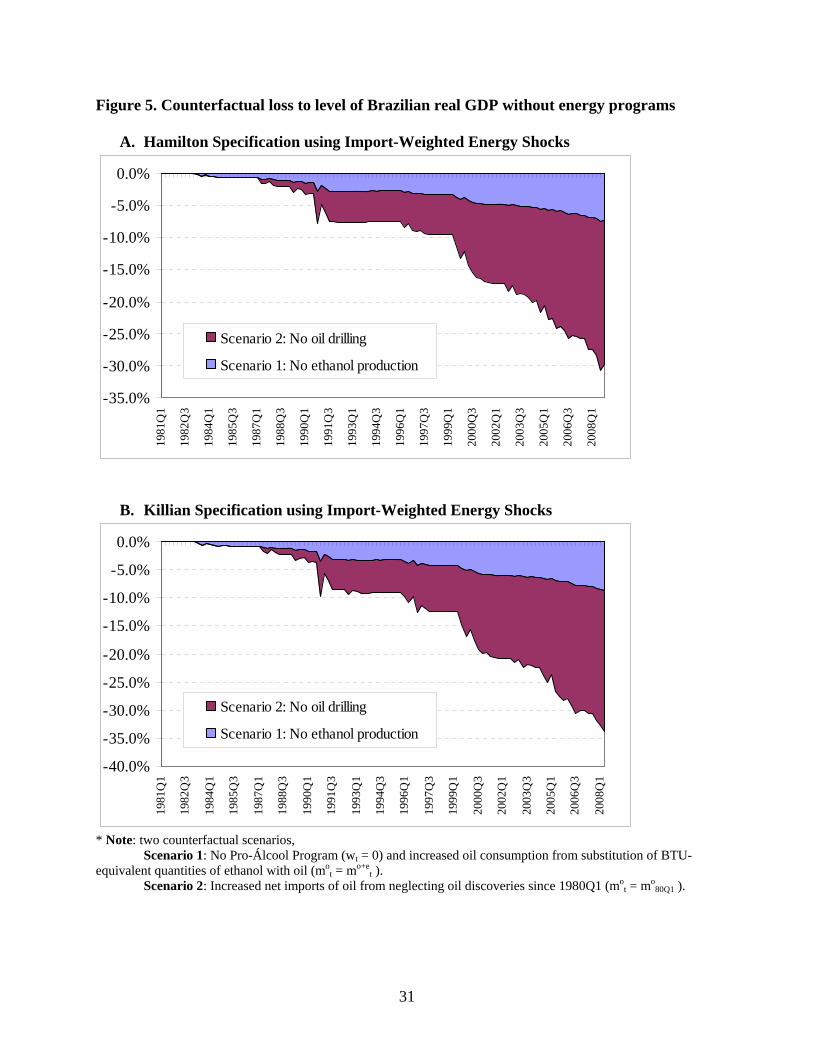
Figure 5. Counterfactual loss to level of Brazilian real GDP without energy programs
A. Hamilton Specification using Import-Weighted Energy Shocks
-35.0%
-30.0%
-25.0%
-20.0%
-15.0%
-10.0%
-5.0%
0.0%19
81Q
1
1982
Q3
1984
Q1
1985
Q3
1987
Q1
1988
Q3
1990
Q1
1991
Q3
1993
Q1
1994
Q3
1996
Q1
1997
Q3
1999
Q1
2000
Q3
2002
Q1
2003
Q3
2005
Q1
2006
Q3
2008
Q1
Scenario 2: No oil drilling
Scenario 1: No ethanol production
B. Killian Specification using Import-Weighted Energy Shocks
-40.0%
-35.0%
-30.0%
-25.0%
-20.0%
-15.0%
-10.0%
-5.0%
0.0%
1981
Q1
1982
Q3
1984
Q1
1985
Q3
1987
Q1
1988
Q3
1990
Q1
1991
Q3
1993
Q1
1994
Q3
1996
Q1
1997
Q3
1999
Q1
2000
Q3
2002
Q1
2003
Q3
2005
Q1
2006
Q3
2008
Q1
Scenario 2: No oil drilling
Scenario 1: No ethanol production
* Note: two counterfactual scenarios, Scenario 1: No Pro-Álcool Program (wt = 0) and increased oil consumption from substitution of BTU-equivalent quantities of ethanol with oil (mo
t = mo+et ).
Scenario 2: Increased net imports of oil from neglecting oil discoveries since 1980Q1 (mot = mo
80Q1 ).
31

Figure 6. United States Net Oil Import Share, 1975-2008Q1
0
0.1
0.2
0.3
0.4
0.5
0.6
0.719
74M
01
1976
M04
1978
M07
1980
M10
1983
M01
1985
M04
1987
M07
1989
M10
1992
M01
1994
M04
1996
M07
1998
M10
2001
M01
2003
M04
2005
M07
2007
M10
U.S. net import
U.S. counterfactual netimport (m=14%)
Source: EIA.
32
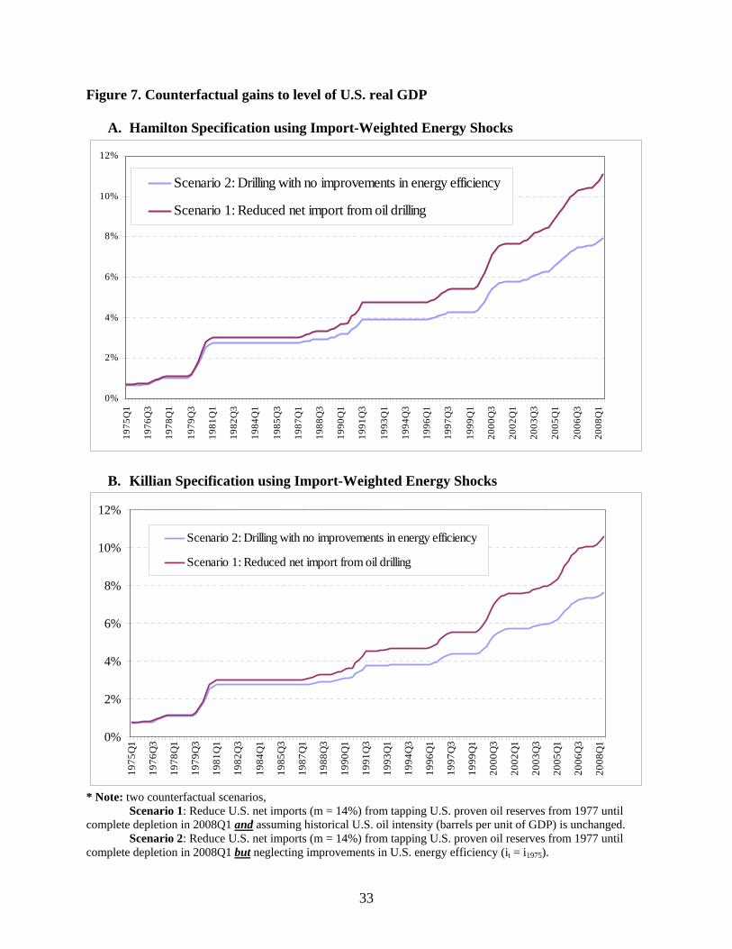
Figure 7. Counterfactual gains to level of U.S. real GDP
A. Hamilton Specification using Import-Weighted Energy Shocks
0%
2%
4%
6%
8%
10%
12%
1975
Q1
1976
Q3
1978
Q1
1979
Q3
1981
Q1
1982
Q3
1984
Q1
1985
Q3
1987
Q1
1988
Q3
1990
Q1
1991
Q3
1993
Q1
1994
Q3
1996
Q1
1997
Q3
1999
Q1
2000
Q3
2002
Q1
2003
Q3
2005
Q1
2006
Q3
2008
Q1
Scenario 2: Drilling with no improvements in energy efficiency
Scenario 1: Reduced net import from oil drilling
B. Killian Specification using Import-Weighted Energy Shocks
0%
2%
4%
6%
8%
10%
12%
1975
Q1
1976
Q3
1978
Q1
1979
Q3
1981
Q1
1982
Q3
1984
Q1
1985
Q3
1987
Q1
1988
Q3
1990
Q1
1991
Q3
1993
Q1
1994
Q3
1996
Q1
1997
Q3
1999
Q1
2000
Q3
2002
Q1
2003
Q3
2005
Q1
2006
Q3
2008
Q1
Scenario 2: Drilling with no improvements in energy efficiency
Scenario 1: Reduced net import from oil drilling
* Note: two counterfactual scenarios,
Scenario 1: Reduce U.S. net imports (m = 14%) from tapping U.S. proven oil reserves from 1977 until complete depletion in 2008Q1 and assuming historical U.S. oil intensity (barrels per unit of GDP) is unchanged.
Scenario 2: Reduce U.S. net imports (m = 14%) from tapping U.S. proven oil reserves from 1977 until complete depletion in 2008Q1 but neglecting improvements in U.S. energy efficiency (it = i1975).
33

Data Appendix. Figure A1. Petroleum real price indices: Raw data and Kilian SVAR
0
50
100
150
200
250
1980
Q1
1981
Q4
1983
Q3
1985
Q2
1987
Q1
1988
Q4
1990
Q3
1992
Q2
1994
Q1
1995
Q4
1997
Q3
1999
Q2
2001
Q1
2002
Q4
2004
Q3
2006
Q2
2008
Q1
Oil price index
Oil price index (no globaldemand shocks)
Note: Price indices 1975=100. Kilian SVAR series corresponds to the predicted value for oil prices from the SVAR plus two of the three structural shocks: supply and precautionary demand. Figure A2: Brazilian net imports (mo
t) and counterfactual net imports (mo+et)
0%
10%
20%
30%
40%
50%
60%
70%
80%
1980
Q1
1982
Q1
1984
Q1
1986
Q1
1988
Q1
1990
Q1
1992
Q1
1994
Q1
1996
Q1
1998
Q1
2000
Q1
2002
Q1
2004
Q1
2006
Q1
2008
Q1
Net_import
Counterfactualnet Import
Source: IPEA, Brazil’s government, www.ipea.gov.br.
34