NBER WORKING PAPER SERIES

CONTRACEPTION AND FERTILITY:

HOUSEHOLD PRODUCTION UNDER UNCERTAINTY

Robert T. iichael and Robert J. Willis

Working Paper No. 21.

CENTER FOR ECONOMIC ANALYSIS OF II1ThAN BEHAVIOR AND SOCIAL INSTITUTIONSNational Bureau of Economic Research, Inc.261 Madison Avenue, New York, N.Y. 10016

December, 1973

Preliminary; Not for Quotation

NBER working papers are distributed informally and in limitednumber for coimnents only. They should not be quoted without written

permission.

This report has not undergone the review accorded official NBERpublications; in particular., It has not yet been submitted for approvalby the Board of Directors.

ICONTRACEPTION AND FERTILITY:

HOUSEHOLD PRODUCTION UNDER UNCERTAINTY

Robert T. Michael and Robert J. Willis

Table of Contents

I Introduction 1

II The Analytical Framework 8

III i. Birth control and the dis-tribution of fertility out-comes 9

ii. Benefits of fertility con-trol 17

iii. Costs of fertilitycontrol 25

iv. Optimal fertility controlstrategy 32

IV Pure and Mixed Contraceptive

Strategies 35

V Contraception and Fertility Out-comes 41

VI The Diffusion of the Pill 59

November 1973

This study has been supported by a population economics programgrant to the NBER from the National Institute of Child Health and Human

Development, PHS, Department of HEW. This paper is not an official NBERpublication since it has not been reviewed by the NBER Board of Directors.We want to thank Lee A. Lillard for useful suggestions and C. Ates Dagli,Kathleen V. McNally and Joan Robinson for their careful research assis-

tance.

This paper was prepared for presentation at a November 1973 NBERConferenée on Research in Income nd Wealth and is forthcoming inhold Production and Consumption, NBER Income and Wealth Conference Volume.

S

I Introduction

Over the past century fertility behavior in the United States

has undergone profound changes. Measured by cohort fertility the

average number of children per married woman has declined from about

55 children at the time of the Civil War to 2.4 children at the time

of the Great Depression. it is seldom emphasized however that an even

greater relative change took place in the dispersion of fertility a—

mong these women: the percentage of women with, say, seven or more

children declined from 36% to under 6%,1 While students of population

have offered reasonably convincing explanations for the decline in

fertility over time, they have not succeeded in explaining the fluc-

tuations in the trend and have made surprisingly little effort to ex-plain the large and systematic decline in the dispersion of fertilityover time. In this paper we attempt to study contraception behaviorand its effects on fertility. One of the effects on which we focus

considerab]e attention is the dispersion or variance in fertility.

Our analysis is applied to cross—sectional data but it also provides

an explanation for the decline in the variance of fertility over time.

1These figures are taken from the report of the President'sCommission on Population Growth and the American Future (see Taeuber1972). They are indicated below in Table I—i.

S

S The study of fertility behavior has received increasing atten-

tion by economists in the past few years. Much of this analysis has

been conducted in the context of the new theory of consumer behavior

pioneered by Becker (1965) and Lancaster (1966). The work on fertili-

ty behavior complements many other studies dealing with aspects of

household production. One of the specific topics in the fertility

literature has been the relationship between child bearing and several

life cycle production decisions such as marriage, schooling, women's

career choices, life cycle time and money allocations and so forth.

A second and related topic of the economics of fertility behavior is

the tradeoff in household production between the family's number of

children and the expenditure of resources per child, particularly the

expenditure of time devoted to children at the pre—school age. A

third focus of this research has been the fertility demand function——

the form and stability over time and across groups of the household's

demand function for children.2

Nearly all of these studies of household fertility behavior as-

sume that the household can produce exactly the number of children

it wants, costlessly and with certainty. We have previously pointed

out that costly fertility control operates as a subsidy to child bearing,

2For a thorough model of fertility demand and the quantity—quality trade—off s in the context of a static framework see Willis(1973). For an extensive set of papers pertaining to topics in fer-tility behavior see the two NBER conference volumes New Economic

Approaches to Fertility and Marriage, Family Human Capital andtility, Schultz (ed.) (1973) and (1974). These volumes indicate, wethink, that much of observed fertility behavior is amenable to eco—

nomic analysis.

lowerimg the marginal cost of havingadditional children (see Willis

1971) and we have suggested a frameworkfor analyzing the household's

fertility control decisions (see MIchael 1973). In this paper we con-

sider the household's fertility control behavior both in terms of the

selection of specific fertility control strategies (the costs and bene-

fits of specific contraceptivetechniques) and in terms of the effects

of different control strategies on household fertility.

One could introduce fertility control costs into.adetejnjgj

model of fertility behavior by treating these costs as transaction

costs associated with acquiring any given level of fertility. In this

framework, the household can select any number of children with cer-

tainty provided it pays the requisite costs of fertility control. As—

sinning that total fertility control costs are larger the smaller the

number of children chosen, the positive marginal cost of fertility con-

trol raises average fertility by acting as a subsidy to childbearing.

In this paper, we have treated the costs of fertility control in a

somewhat different framework. We have adopted a model in which the

household can select with certaintyany particular monthly probability

of conception,3 but in which the household's actual fertility, N, is a

stochastic variable. By selecting and producing a particular monthly

3The probability is bounded by zero add by the probability im-plied by natural or intrinsic fecundability, say, a probability ofabout 0.2 per month.

S

probability of conception, the household selects a distribution of

fertility outcomes. The mean ofthat distribution is its expected

fertility; its varianceindicates the uncertainty that the house—

hold faces.

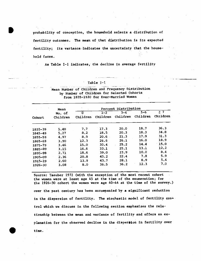
As Table I—i indicates, the decline in average fertility

Table I—i

Mean Number of Children and Frequency Distribution

by Number of Children for Selected Cohortsfrom 1835—1930 for Ever—Married Women

MeanNo. of

Percent Distribution70 1—2 3—4 5—6

Cohort Children Children Children Children Children Children

1835—39 5.40 7.7 17.3 20.0 18.7 36.3

1845—49 5.27 8.2 18.5 20.3 18.3 34.8

1855—59 4.97 8.9 20.6 21.3 17.9 31.3

1865—69 3.90 12.3 26.6 26.1 16.0 18.9

1875—79 3.46 15.0 30.4 25.2 14.4 15.0

1885—89 3.15 16.6 33.1 25.1 13.1 12.2

1895—99 2.71 18.6 39.0 23.9 10.0 8.4

1905—09 2.36 20.8 43.2 22.4 7.8 5.9

1915—19 2.60 13.9 43.7 28.1 8.9 5.4

1926—30 3.08 8.0 36.5 36.2 12.3 7.0

Source: Taeuber 1972 (with the exception of the most recentat the time of the enumeration; for

the 1926—30 cohort the women were age 40—44 at the time of the survey.)

over the past century has been accompanied by a significant reduction

in the dispersion of fertility. The stochastic model of fertility con+

trol which we discuss in the following section emphasizes the rela-

tionship between the mean and variance of fertility and offers an ex-

planation for the observed decline in the disperàton in fertility over

time.

cohort

I

.

the women were at least age 45

Child rearing is anexceptionally costly activity, both in terms

of direct dollar outlays and forgone time and human capital.,4Probably

few events in one's lifetimeaffect subsequent behavior more exten-

sively than having a child. While other important life cycle decisions

such as marriage and career choice are subject to considerable uncer—

tainty, the uncertainty generally pertains to the quality or the char-

acteristics of the object of choice.Uncertainty about the charac-

teristics of the prospective child alsoexist of course, but in addi-

tion there exists the uncertainty which we are emphasizing__uncertainty

about the acquisition of a child itself.

At the individual household levelthis uncertainty about the num-

ber of children affects at least three aspects of behavior. First,

it may affect decisions about the expenditures of resources on exist—

Ing. children——if ordinary substitution between quantity and quality

is relevant to children, thennot knowing the final number of children

may affect the household's expenditure decisions on its first—born

children. Second, there exists Sbtitti0 between expenditures on

4For estimates of the direct costs of children see Cain (1971) orReed and McIntosh (1972). Lindert(1973) presents a useful discussion

of existing evidence on various aspects of the costs of children. Michaeland Lazear (1971) emphasize the potenttal cost of children in terms offorgone human capital and Mincer and Polachek (1974) estimate the de-preciation in the mother's human capital related to her noninarket childrearing activity.

.

children and on other household goods and *eriiceB and also between

expenditures over time. So uncertainty about the number of children,

and about the timing or spacing of children, can be expected to af-

fect the composition and timing of consumer expenditure and savings

behavior. Third, because of important interactions with other house-

hold production and with the relative value of family member's time,

uncertainty about the number of children may have effects on the parents'

occupation choices, schooling decisions and general orientation toward

market and household activities.

At the aggregate level, positive fertility control costs and the

stochastic nature of fertility behavior affect the observed mean and

variance of fertility. The size and growth rate of the population

affect the age distribution of the population and the rate of growth

and the composition of the economy's output.5 The variance in fer-

tility, on the other hand, influences the distribution of income and of

wealth. If uncertainty about fertility outcomes affects household

investment and savings decisions, it may have an important influence on

the distribution of inherited wealth across generations.

5See Kelley (1972) for a recent discussion of population growthand economic progress. See Kuznets (1960) and other essays in Demo—graphic and Economic Change in Developed Countries for discussions of

the effects of population on output employment and demand.

.

These considerations are not the focus of our paper, but we

think the points we emphasize here——thecosts of fertility control,

fertility as a stochastic process and therelationship between the

mean and variance of fertility——have; important Implications for the

level and distribution of the ecónonty's wealth. We do not explore

these aggregate relationships, nor do we resolve many of the more

esoteric problems which we encounter in oir analysis. We do how-

ever attempt to Integrate into an analysIs of contraceptive choice

and optimum fertility behavior the constraints imposed by biological

limitations and resource (or economic) limitations. We indicate

how the choice of contraceptive technique affects the observed mean

and variance of fertility. We also analyze the choice of contracep-

tive technique, in particular the adoption of the new oral contra-

ceptive in the United States in the first half of the l960's.

.

.

II The Analytical Framework

The theory of the choice of a fertility control strategy treats

the fertility goals of the household as given, wbile the economic theory

of fertility demand focuses on the factors which determine thesegoals.

If fertility control Is costly, however, these costs as well as the re-

source costs of bearing and rearing children influence the couple's

choice of fertility goals. The link between the theory of the choice

of birth control technique and the theory of fertility behavior is

provided by assuming that the household maximizes its lifetime utility

subject to the constraint of a fertility control cost function as

well as the conventional economic resource constraint. The fertility

control cost function is simply the combination (the envelope) of

least—cost birth control strategies for all possible fertility outcomes.

In this section we describe a stochastic model of reproduction,

emphasizing the relationship between the mean and variance of fertility

outcomes. We then discuss the economic benefits and costs of fertility

control and conclude with an exposition of the optimal fertility control

strategy.

______ .i Birth control and the distribution of fertility outcomes

The number of children born to a couple and the pace at which

these children are born isultimately constrained by the fact that

reproduction is a biological process. The observed reproductive

behavior of an individual, womanover her life cycle may be regarded

as the outcome of this biological process as it is modified by non—

volitional social and cultural factors and by the effects of deli-

berate attempts to control fertility. In the past two decades, the

nature of the biological constrainton fertility choices has been

greatly clarified and given rigorous expression in stochastic models

of the reproductiveprocess by Henry, Potter, Perrin and Sheps, and

others. The basic reasoningunderlying these models and their main

implications for average fertility were recently summarized by Key—

fitz (1971).

These models suggest that the number of children a woman bearsduring her lifetime is a random variable whose mean and variance de-

pend on her (and her partner's) choice ofa fertility control strategy.

In this section we draw heavily on this literature in order to pre-

sent, under simplifying assumptions, analytical expressions for the

mean and variance of live births as a function of two sets of para-

meters, one representing the coupl&s biological characteristics and

the other Its fertility controlstrategy.

The simple observation that it takes a random amount of time to

produce a baby provides the point of departure for recent biological

models of fertility. Suppose that a woman faces a probability p'of

conceiving in a given month. If that monthly probability of con-

ception Is constant over time, the probability that she will con-

ceive in exactly the jth month (j — 1,2,,,,) is p(1—p)'vhere

(1—p)1is the probability that she fails to conceIve in the first

j—i months. Employing the demographer's term "conceptive delay",

i.e. the number of months, v , it takes a fecund woman to conceive,

the random variable v is distributed geometrically with meanp2 26and variance a i," (l-p)/p

Once a woman conceives she becomes sterile during her preg-

nancy and the anovulatory period following pregnancy. The lenbh

of the sterile period, s , is also a random variable whose value de-

pends on the type of pregnancy termination (i.e., fetal loss or still-

birth or live birth) and on the physiological and social factors

(e.g., age, parity, breast feeding practices, time to resumption of

sexual activity) which determine the length of the anovulatory period

following each type of pregnancy termination. For simplicity, we

shall assume that all pregnancies terminate in a live birth and

that the length of the sterile period, s, is of fixed, nonrandom

length.7 The length of one reproductive cycle——the number of months

6See Sheps (1964) for a derivation of this result, It shouldbe noted that conceptive delay is defined to be zero months,if thewoman conceives in the first month.

7See Perrin and Sheps (1964) for a model in which pregnancyterminations other than live births are allowed and the sterileperiod associated with each type of pregnancy is of random length.Compared with the formulas we shall present, the Perrin and Shepsmodel implies a smaller mean and larger variance in the number oflive births a woman has over her reproductive span.

— ii —

.it takes a fecund woman to become pregnant, give birth and revert

to a fecund, non—pregnant status——can be expressed as t v + s,

a random variable with mean 'j i + and variance a2 a2t V t v•The number of children the woman bears during a lifetime, say

a reproductive span of T months, depends on the number of repro-

ductive cycles completed during this period. Since each cycle is

of random length, the woman's fertility will also be a random vari-

able. The probability distribution of the number of births can be

represented in a simple way if the model of reproduction is repre-

sented as a Markov renewal process. In order to qualify as a re-

newal process, the intervals between successive births must behave

as independent, identically distributed random variables (Potter, 1970).

To meet these qualifications, it is necessary to assume that all of

the parameters of the reproductive process (i.e., p and s) are con-

stant over time and that the reproductiveperiod, T, is sufficiently

long (i.e., infinity). Assuming reproduction to be a renewal pro-

cess, the distribution of the number of births N isasymptotically

8normal with mean

T/llt (1)

8See Sheps and Perrin (1966) who warn that the asymptoticnormal distribution above does not adequately approximate theexact probability of N for the relevant (finite) range of T. Inanother paper Perrin and Sheps (1964) suggest more accurate ap-proximate expressions for the first two moments of N. Since thequalitative implications of these approximations are quite simi-lar to those of the more exact approximations, it does not seemnecessary to encumber the discussion with more complicated ex-pressions for mean and variance. A more serfous problem is sug-gested by Jam (1968) who fund that the actual mean of naturalfertility tends to fail progressively below the theoretical. mean,.given by the Perrin—Sheps model as T increases, while actualvariance rises progressively above the theoretical variance.

— IL —

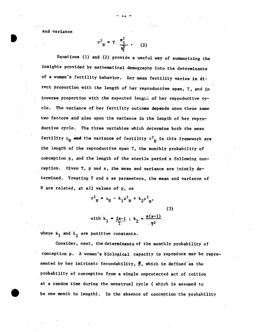
and variance

I a2 T•

N (2)

Equations (1) and (2) provide a useful way of suimnarizing the

insights provided by mathematical demography into the determinants

of a woman's fertility behavior. Her mean fertility varies in di-

rect proportion with the length of her reproductive span, T, and in

inverse proportion with the expected lengLi1 of her reproductive cy-

cle. The variance of her fertility outcome depends upon these same

two factors and also upon the variance in the length of her repro-

ductive cycle. The three variables which determine both the mean

fertility N and the variance of fertility a2N in this framework are

the length of the reproductive span T, the monthly probability of

conception p, and the length of the sterile period s following con-

ception. Given T, p and s, the mean and variance are jointly de-

termined. Treating T and s as parameters, the mean and variance of

N are related, at all values of p, as

a2 p —kp2 +ki3N N 1 N 2 N'

(3)

with k 2s—1 ; k s(sl)1

T2

where k1 and k2 are positive constants.

Consider, next, thedeterininantsof the monthly probability of

conception p. A woman's biological capacity to reproduce may be repre-

sented by her intrinsic fecundability, 0, which is defined as the

probability of conception from a single unprotected act of coition

at a random time during the menstrual cycle ( which is assumed to

be one month in length). In the absence of conception the probability

p that she will conceive during a given month is then equal to the

product of and her monthly frequency of coitlonc,9 Demographers

frequently discuss "natural fertility" defined, following Henry (1961),

as the number of live births a woman expects to have in a reproductive

lifespan of T months In the absence of any deliberate attempt to control

fertility. If we suppose there is some "natural" level of coital fre-

quency for a given couple, then ê = p*, the couple's monthly pro-

bability of conception in the absence of any fertility control. We

will generally assume = 7 and = 0.03 (see Tietze, 1960), hence we

will asste that p* = 0.2. Given p* and given the reproductive time

span T and the length of the period of infertility s, the mean and

variance of natural fertility, )J and cii, are defined by equations

1 and 2.

Variations across couples in the monthly probability of concep-

tion p may result from variations in fecundity—-which affect '$-— or

from variations in coital frequency. Variations may also result from

contraception. If the adoption of a particular contraceptive strategy

i reduces the monthly probability of conception by e1 percent, then

i= p* (—) Oe1*1.So the couple's actual monthly probability of conception p1 Is deter-

mined by Its fecundity, coltal frequency and contraceptive practice.

As we emphasized above, to qualify as a Markov renewal process

of reproduction the monthly probability p1 is assumed to be constant

Intrinsic fecundability is discussed In the demographic liter-ature, which contains an empirical justification for expressing p asapproximately proportional to c over the relevant range of variationin monthly frequency of coition.

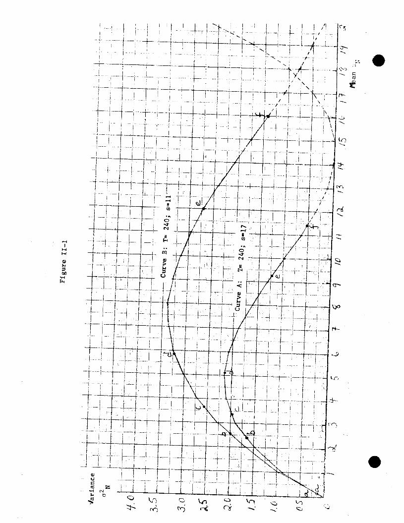
for all fertile months in the reproductive timespan of

T months. Under these circumstances figure lI—i indicates the re-

lationship between the mean and variance of fertility as summarized

in equation 3. Curve A assumes T—240 months ( a reproductive span

of 20 years) and s=17 months (a 17 month period of sterility following

conception, see Keyfitz 1971). Each point on Curve A corresponds to

a different constant monthly probabil'ty of conception ranging from

pO.O ( the origin) to p"O.2 (point f on the curve).10 Curve B in

figure 11—i depicts the same relationship under the assumption that

T equals 240 months and s equals only 11 months.

Suppose a couple, at the time of their marriage, were charac-

terized by the parameter values T 240 months, s 17 months and p*

•0.2. They would then face an ex ante distribution of fertility out-

comes with a mean of 11.4 births and a variance of 0.5 (point f on

Curve A in figure Il—i). The couple could, however, alter this ex-

pected outcome by adopting a strategy of fertility control which

lowered their constant monthly probability of conception below p*.

If, for example, the couple selected a contraceptive technique with

efficiency e1 0.5, then their monthly probability would be p1

p*(i_O.S) 0.1 and their ex ante distribution of fertility outcomes

would have a mean of 9.2 births and a variance of 1.2 (point e on

'°For example, if p'O.OOO8 then p = 0.19 births and 0.18

which is shown as point a on Curve A. he values of p which correspond

to points a,b,c,d,e,f in the figure are 0.0008, 0.0120, 0.0182, 0.0336,

0.1000, 0.2000 respectively. These values refer to specific forms

of fertility control and are discussed below.

.

.

Figure ri—i

an , .

— 15 —

Curve A). Thus the couple affects its expected fertility and its

uncertainty about the number of its births by its selection of a

contraceptive strategy."

Both the contraceptive technique used and the care with which

it is used can affect e1 which in turn determines p1. In general,

the couple can also affect p1 by altering its frequency of coition,

c, and can also affect the distribution of fertility outcomes for

any given p1 by altering the length of the reproductive period at

risk, T, through decisions about the age at marriage and the age at

which either partner is sterilized2 So the full range of fertility

control strategies includes considerations other than the choice of

contraceptive method, but it is the contraceptive choice on which

"In reality, it is plausible to suppose that the frequency ofcoition and contraceptive efficiency will tend to vary over time toaccommodate a couple's preferences for childspacing as well as fortotal number of births, or to accommodate any changes in their fer-tility goals.

It is also plausible to suppose that the choices of c and e1will be conditioned on past pregnancy and birth outcomes. Thus, ingeneral, the values of p in a given month will tend to be a functionof time (i.e., age), past reproductive history (I.e., parity) andrandom fluctuations in variables that detemnine fertility goals.

Unfortunately, the analytical simplicity of considering thestochastic model of reproduction as a renewal process is lost underthese conditions. While it is possible to write out probability state-ments in which a couple's contraceptive strategy (i.e., its choices ofc and e) is defined conditional on all possible fertility outcomes ateach period of time, it is not possible to derive the implications ofthe resulting stochastic process for completed fertility outcomes usinganalytic methods. Moreover, the dynamic optimization problem involvedin selecting a contraceptive strategy that maximizes a couple's expectedutility under conditions of uncertainty may itself be analytically in-tractable. At this stage, it appears wiser to minimize the formal dif—

. ficulties , thus the contraceptive parameters, c and as well as

the biological parameters, and a, are assumed to remain constant over

time.12

Interruptions of exposure within the time span T caused by cessa—

tions of sexual relations due to divorce or separation are ruled out by the

assumption that the parameters of the process remain constant over time.

— 16 —

Swe viii. focus. By selecting contraceptive strategy i which yields

a monthly probability of conception p1, the couple has in effect

selected a particular ex ante distribution of its fertility outcomes.

The mean of that distribution Is N and Its variance is a2 WeN1

will assume for now that the couple is constrained to a pure contra-

ceptive strategy, defined as the adoption of some form of fertility

control which aets p at some fixed level (during fertile periods) for

the entire reproductive span.

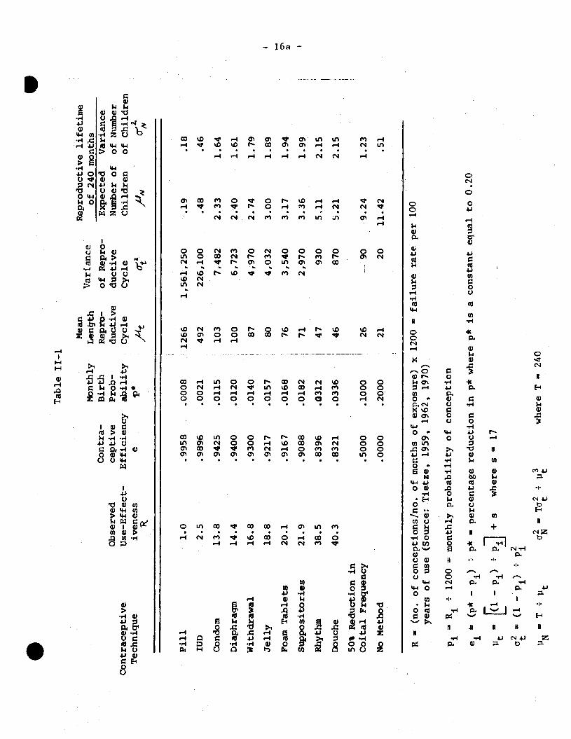
From studies of the average contraceptive failure rates of various

contracpetive techniques, the efficiency—in_use of each technique

can be computed. Table 11—1 lists the contraceptiveefficiency e1 and

the implied monthly probability of conception for several contra-

ceptive techniques.13 The table also computes for each technique the

mean and variance of the length of the reproductive cycle and the mean

and variance of the fertility outcomes in a 20 year reproductive span.

Thus, given the biological constraint on its fertility (e.g. Curve A

in figure 11—i) the couple can determine the expected distribution of

its fertility ( Its UN and aj) by selecting a contraceptive strategy

which achieves any particular p . The various points labeled on Curve AI

indicate the mean and variance of births associated with various con-

traceptive techniques (point a: pill; b: diaphragm; c. suppository; d: rhythm;

e: 50% reduction in coital frequency and no other contraception; f:no

fertility control).

'3The estimates of contraceptive efficiency were compiled byMichael (1973) from the demographic literature ( see especially Tietze(1959) and (1962) ). See Michael (1973) for a discussion of the dif-ficulties In estimating and the hazards in using this comparativelist of the efficiency of contraceptive methods. In particular, notethat these values represent average observed use—effectiveness andwill in general be affected by the intensity and care with which theyare used.

. Table IT—i

R = (n

o. o

f conceptions/no, of months of exposure)

years of use

(Sou

rce:

Tietze, 1959, 1962, 1970)

Pj = R1

÷

1200

= m

onth

ly probability of conception x 1200 — f

ailu

re rate per 100

ei

(p* — p1

) p* — pe

rcen

tage

reduction in p* where p* is a constant equal to 0.20

t_ [i_j p

+s

wheresl7

(1 —

+ p

= T

= T

a w

here

T — 240

Contraceptive

Technique

Observed

Use-Effect-

iven

ess

Con

tra-

ce

ptiv

e E

ffic

ienc

y e

Monthly

Birth

P rob-

ability

Mea

n L

th

Rep

ro-

Var

ianc

e of

Rep

ro-

Rep

rodu

ctiv

e lif

etim

e of

240

m

onth

s E

xpec

ted

Var

ianc

e du

ctiv

e du

ctiv

e N

umbe

r of

of

Num

ber

Cyc

le

Cyc

le

Chi

ldre

n of

Chi

ldre

n Ju

t 0_

ta

PIY

C

Pill

1.0

.9958

.0008

H 1266

1,561,250

.19

.18

IUD

2.5

.9896

.0021

492

226,100

.48

.46

Con

dom

13.8

.9425

.0115

103

7,482

2.33

1.64

Diaphragm

14.4

.9400

.0120

100

6,723

2.40

1.61

Withdrawal

16.8

.9300

.0140

87

4,970

2.74

1.79

Jelly

18.8

.9217

.0157

80

4,032

3.00

1.89

Foam Tablets

Supp

osito

ries

Rhythm

20.1

21.9

38.5

.9167

.9088

.8396

.0168

76

.0182

71

.0312

47

3,540

2,970

930

3.17

3.36

5,11

1.94

1.99

2.15

Dou

che

40.3

.8

321

.033

6 46

87

0 5.

2].

2.15

50

% R

educ

tion

in

Coi

tal

Freq

uenc

y .5

000

.100

0 26

--

-90

9.24

1.

23

No

Met

hod

.000

0 .2

000

21

20

11.4

2 .5

1

a'

.In this framework the number of children born to a couple

is a random variable which results from a stochastic process. Ex

post, the couple has only one number of children N. But the couple

cannot determine its number of children with absolute certainty.

Rather it can select any particularvalue of p, the monthly proba-

bility of conception, which yields a particular distribution of fer-

tility outcomes summarized by the distribution's mean and variance.

So long as we assume that the couple selects one value for p

and retains that particularmonthly probability of conception for

all the fertile months in the 20 year span——an assumption we will

characterize as a "pure"strategy model—-. the couple cannot alter its

expected fertility UN without also altering the variance a. In short,

the pure strategy model restricts the couple to the biological con-

straint (Curve A in figure lI—i if T=240, s=17). Before we relax the

assumption of the pure strategy we discuss the determinants of the

couple's choice of Its most preferred position along the biological

constraint. We consider in turn the benefits and the costs of fertility

control.

ii Benefits of fertility_control

Recent economic theories of household behavior postulate the ex-

istence of several constraints (e.g., a money income constraint, a time

constraint, production function limitations) on the household's maxi-

mization of utility. The utility is derived from a broad set of de-

siderata which are produced by the household itself In the nonmarket

sector, using purchased market goods and services and the household

Imembers' own time as the inputs in the production.'4 These pro-

duction functions emphasize the distinction between the household's

wants (the output) and the means used to satisfy these wants (the

goods and time inputs).I

Willis (1973) recently utilized the household production frame-

work to formulate an economic model of hutn fertility control. We

will generalize a simple version of Willis' model to deal with im-

perfect and costly fertility control. The formal analysis is con-

ducted in a static lifetime framework, although we informally sug-

gest how the implications of the model might be altered in a more

15dynamic or sequential decision making framework.

In Willis' model it is assumed that the satidfaction parents

receive from each of their N children is represented by Q1, Q2

and the satisfaction from other sources of enjoyment is represented

by S. The Q1, or "quality" of each child, and the other composite

commodity S are produced within and by the houshold using the family

members' time and purchased market goods as inputs. The household

production functions characterize the relationship between inputs of time and

goods and the outputs of Q and S. Assuming (among other things) that

14See Becker (1965) and Lancaster (1966) for early statements of

this model. Several monographs and articles in recent years, notablythrough NBER, have utilized this framework. For a recent brief survey

see Michael and Becker (1973).

15

For a model of sequential decision making regarding contraceptive

behavior in a heterogenous population see Heckman and Willis (1973).

.parents treat all their children alike, the total amount of child—

services C may be written as a product of quality per child Q and

the number of children N: C = NQ. It is assumed that Q Is positively

related to the amount of time and market goods devoted to each

child——Q Is perhaps best considered an Index of the child's human

capital. The household's preferences for number and quality of

children and for all other forms of satisfaction are summarized

by its lifetime utility function

U U(N, Q, S). (4)

The household's capacity to produce C and S Is limited by its

lifetime real income and by the quantity of its nonmarket time. Willis

(1973) discusses in detail the relationship between the relative prices

of N and Q, and considers how various changes in the household's char-

acteristics and circumstances would be expected to affect its demand

for N, Q and S.

One important implication of the economic model of fertility

demand should be noted. From an assumption that children are relatively

time—Intensive in the wife's time (i.e. C—production requires more of

the wife's time per dollar of goods—input than does S-production), the

relative cost of C rises as the wife's wage rate rises. Hence the

cost of both number of children N and quality of children Q also rises

with the wife's wage rate. If the relative price of N rises with the

wife's wage rate, then abstracting from the change in income, women with

higher wages (or higher levels of education) are expected to have lower

fertility. This is the basis of the1'ost of tlme"hypothesls (Ben—Porath,

.

1973) which has, since Mincer's pioneering paper (Mincer, 1963), re-

ceived much attention as an explanation for the observed negative

relationship between the wife's wage and her fertility.

The household's lifetime money income constraint, its time

contraint and its production function constraints can be treated

as a single constraint on the household's lifetime full real income, I.

Defining the marginal costs of childservices and the composite

other commodity ir, the formal optimization problem characterizing

the household's choice is the maximization of the utility function

(equation 4) subject to the full real income constraint.

max UT (N, Q, S) — x[i— q,(ir,,rJ} (5)

where A is the Lagrangean multiplier. This optimization problem

assumes that the household can costlessly and with certainty select

any number of children (N) it wishes and can achieve any given level

of the child's human capital (Q) it chooses.

To relax this assumption, we consider the benefits to the house-

hold of achieving any given number of children. Suppose the household

had the utility function and the full real income constraint indicated

in equation 5 but that the household was endowed with some arbitrary

number of children N' where N' — 0, 1, ,.. (To simplify the mathema-

tics N' will be treated as a continuous variable.) Given its arbi-

trary N', the household's only remaining choices would be the optimal

values of child quality, Q, and other satisfaction, S, which must be

chosen subject to the lifetime full real income constraint. If N and

Q as well as N and S are substitutes in terms of the parents' preferences,

-- h.L —

.the levels of both Q and S will tend to fall as N' is increased. This

azalysis implies that sub—optimal values of Q and S would be chosen

if fertility were arbitrarily constrained. Q and S would tend to be

larger than (or smaller than) the optimal values, Q* and S*, as the

arbitrarily constrained level of fertility, N', is smaller (or larger)

than the freely chosen desired level of fertility, N*. 16

This hypothetical experiment of assigning some arbitrary N to

the household is equivalent to maximizing equation 5 while treating

N as a parameter, for all possible values of N, Such an exercise

yields the household's net utility level as a function of its assigned

level of fertility N' and the economic variables. Written as an im-

plicit function the net utility, V, is

V V(N; I, (6)

For each arbitrarily assigned value of N' there is a maximum

achievable level of utility, obtained by the appropriate mix of Q and

S. By definition, the maximum value of V, indicated as V*, will be

achieved at the desired level of N (N* = N'), as depicted on Curve A

in Figure 11—2.

16

It should be noted that we are implicitly assuming that thecouple knows In advance what number of children it will have andcan plan accordingly for its level of child quality and S.

.

.

Deviations of fertility from N* in either direction, such as N1 or

N2, result in reduced utility levels such as V1 or V2 in Curve A

of figure 11—2. Given the emphasis in discussions of family plan-

ning on the problem of excess fertility and unwanted births (i.e. N)N*),

it is worth stressing that deficit fertility (i.e. N<N*) may reduce

welfare by at least as mucit as excess fertility.'7

The opportunity cost of deficit or excess fertility (V* —V1 or

V* —V2) is a measure of t1e benefits from improved fertility control.

If in the absence of fertility control the household's fertility would

have been N1 (yielding V1) but with a given level of fertility control

the household achieved N1 (yielding V1 such that V1)V1) then (V* - V1)

— (V* —V1)

—V

—V1

is a' measure of the benefit from that level of

17As indicated above, in the case of deficit fertility quality

per child, Q, would be higher than it would be in the case of optimalfertility or a fortiori for excess fertility. If from some ethicalpoint of view parents are judged to place too little weight on theirchildren's welfare, and if we measure child—welfare by the level ofQ, it could be argued that the effect on Q of deficit fertility reducesor outweighs the parents' welfare loss V* — V1.

V

V4

"2

Figure 11—2

(cr:o)

: (cr2

'V0N1 'V2

fertility control. The utility benefits, then, are the gains in 11—

tility which accrue from moving nearer the optimal allocation of re-

sources which would exist if fertility control were perfect and cost—

less (i.e., N*, * and S*).

We suggest above that the choice of particular values of fer-

tility control parameters such as ei yield particular ex ante distri-

butions of fertility summarized by 1N and a. We can, therefore,

formulate the discussion of the benefits of fertility control in terms

of and c3. For purposes of illustration, suppose the functional

form of equation 6 is quadratic in N:

Va+bN+N2 b>O, c<O (7)

where I, ,r and 11 are held constant. Since the unconstrained maximumC S

of V gives the desired value of fertility, N*, it follows from (7)

that

N*=....(8)

We may now treat N as a random variable and take the expected value of

(7) to obtain:

E(V)a+bJN+ j+ci . (9)

Recall that equation (3) indicates the relationship between a, and

'4' '4 "N where is a cubic function). If E(V) is the valuei i

of equation 9 in the absence of any fertility control, and E(V1) is

its value when fertility control ofe (yielding UN , '4 ) is employed,

i ithen the benefit from fertility control strategy I i E(V1) — E(V).,

If we maximize the expected V (equation 9) with respect to

—(E(V))O=b+cp +p' (10)duN N

.

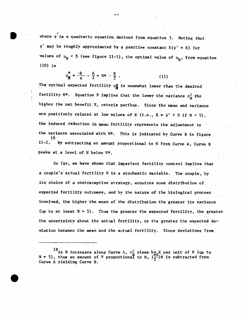
where $, is a quadratic equation derived from equation 3. Noting that

IP' may be roughly approximated by a positive constant K(p' = K) for

values of < 5 (see figure lI—i), the optimal value of , from equation

(10) is

(11)

The optimal expected fertility u is somewhat lower than the desired

fertility N*. Equation 9 implies that the lower the variance the

higher the net benefit V, ceteris paribus. Since the mean and variance

are positively related at low values of N (i.e., K ' > 0 if N < 5),the induced reduction in mean fertility represents the adjustment to

the variance associated with N*. This is indicated by Curve B in figure18

11—2. By subtracting an amount proportional to N from Curve A, Curve B

peaks at a level of N below N*.

So far, we have shown that imperfect fertility control implies that

a couple's actual fertility N is a stochastic variable. The couple, by

its choice of a contraceptive strategy, acquires some distribution of

expected fertility outcomes, and by the nature of the biological process

involved, the higher the mean of the distribution the greater its variance

(up to at least N 5). Thus the greater the expected fertility, the greater

the uncertainty about the actual fertility, or the greater the expected de—

viation between the mean and the actual fertility. Since deviations from

N increases along Curve A, a2 rises bKK per unit of N (up toN — 5), thus an amount of V proportiona to N, (1-)N Is subtracted fromCurve A yielding Curve B.

desired fertility reduce net utility, V, and since higher levels of

expected fertility, N' are associated with greater uncertainty, the

household is induced to reduce its optimal expectedfertility u be-

low its desired fertility N* in order to reduce the uncertainty or

variance a.

iii Costs of fertility control

The costs of fertility control are the amounts of other desir—

ables forgone in achieving the control. These costs include money

costs but also include forgone time, sexual pleasure, religious prin-

ciples, health, and so forth. It is, at best, difficult to measure

these costs empirically. We will Instead discuss some of the deter-

minants of these costs and seek to derive testable hypotheses about

the relationship between observed fertility and contraceptive behavior.

By definition, couples which avoid all the costs of fertility

control have an expected level of fertility p, which is frequently

19referred to as natural fertility. We will assume that costly fer-

tility control strategies are limited to two dimensions: (1) the choice

of contraceptive technique (including regulation of coital frequency) and

'9See the discussion of natural fertility in an earlier section.Throughout section II of this paper we continue to assume that thecouple's fertility control strategy is determined at the outset of theperiod—at—risk of conception and remains constant throughout the re—productive span. uNaturalt fertility results when the age at marriage(which affects T) and the rate of coition, c, are determined withoutregard to effects on fertility.

.

S

(2) the care or intensity with which a given technique is used (i.e.

we assume that the contraceptive efficiency, e1, of the 1th technique

is a variable which may be increased at increased cost to the couple).20

In this section we also restrict the choice of contraception strate-

gies to "pure" strategies. Thus each strategy yields a different monthly

probability of conception and hence a different point on the mean—variance

curve (say, Curve A) in figure lI—i.

Associated with each contraceptive strategy is an opportunity

cost measured by the utility loss associated with the change in behavior

required to implement that strategy. Some strategies cost money, some

coat sexual satisfaction, some cost real or imagined decreases in phy-

sical health. The assumption of utility maximizing behavior implies that

couples will choose the least costly strategy they are aware of in order

to achieve any give level of p which yieUs TMN and its associated cy.

20Thus we rule out for now abortion and sterilization and we

assume age at marriage to be exogenous. To emphasize this restrictionwe will use the term "contraception" in place of "fertility control"in discussing costs, strategies, etc. For a study of abortion as ameans of fertility control see Potter (1972) or Keyfitz (1971) or foran economic analysis see a study in progress by Kramer (1973).

— 27 — .Suppose the couple's cost schedule

for achieving any given p or its fertility outcome is

F =F(UN) (12)

where F is the total cost of achieving N using the least costly

contraceptive strategy. More specifically let the cost of the 1th

contraceptive strategy be the simple linear function

F. =c + =1. (13)

where B is the difference between i, the coupl&s natural fertility,

and PNthe mean of the distribution of its expected fertility while

using strategy i. Thus B is the expected number of births averted.

Equation (13) Imi lies that the total cost of contraception using

the th technique may be divded into two components: (1) a fixed cost,

(c 0) which must be incurred if the jth technique is to he used

.1

.

— 28 —

S

at all, and (2) a variable cost,1 B, which is proportional to thTe num-

ber of births averted by the use of technique i The terrn

is the marginal cost per birth averted.

It is important to stress that the classification of the contra-

ception costs F1 of a given technique as fixed (o<.) or variable B)

is distinct from the classification of costs by their source. An eco—

noniic (e.g. money or time), sociological (e.g. teachings of the Catho-

lic church, deviation from class norms), psychological (e.g. inter-

ference with sexual pleasure, fear of adverse effects on health) or

physiological (e.g. health) cost may he either fixed or variable.

Some factors, however, are more likely to affect1 thanB1 or

vice versa. Lack of contraceptive knowledge, for instance, is often

cited as a reason for imperfect control. To the extent this is true,

it is sensible to suppose that the acquisition of Information about

fertility control methods is costly. A characteristic of the cost of

information is that it does not depend on the amount of use to which

the information is put. It follows that the oosts of information tend

21Each contraceptive strategy involves both the adoption of a con—

traceptive technique and the care and precision In its use. The adop—tion of technique 1 and its careless use results in less efficientcontraception, a lower e1, higher p1 and fewer births averted. Nearlyall contraceptive techniques are capable of achieving a low e1 withcareless use or a high e1 with proficient use.

22The linearity of the cost functions in (13) is not a particular-ly crucial assumption in the sense that the implications to be derivedcould be obtained under less restrictive assumptions.

S

to influence the fixed cost:s of contraception (the , but not23

the marginal costs (the 1's). The cost to a Catholic of violating

the Church's precepts with respect to the use of a contraceptive, for

example, might be a once—and—for—all cost in which case is higher

for Catholics than non—Catholics for all forbidden contraceptive tech-

niques. Alternatively (or additionally), a Catholic may experience

greater guilt the more intensively the technique is used, in which

24case is higher to Catholics than to non—Catholics.

The loss of sexual pleasure occasioned by contraception almost

surely affects only the marginal costs of contraception and not the

fixed costs. Thus, the number of births averted by condoms depends

on how frequently and with what care condoms are used. The most ancient

contraceptive techniques——abstinence or educed coital frequency, and

withdrawal——probably have zero fixed cost and rather high (psychological)

marginal costs. By way of example, consider the choice between re-

duced coital frequency or withdrawal as alternative contraceptive

techniques.

23

This argument should be qualified to the extent that informationis acquired by a process of "learning by doing" or that information de-teriorates with d1susey a process of forgetting. In this case, themarginal cost of the i technique ($.) would tend to shift downwardas the volume of use increases. Analytically, the learning hypothesisand the once—and—for—all hypothesis have the same implication, namely,that the average contraception cost per birth averted decreases as Bincreases.

24The cost to an individual Catholic of violating the Church's

precepts may also be a function of the behavior of other Catholics orof other members of the society at large. Thus, the dynamics of dif-fusion of the pill use among Catholics might be interpreted , in part,as he progressive lowering in the cost of contraception to each mdi—vidual Catholic as he or she sees others using the pill. Of course, theequivocation within the Church itself also presumably lowers the costs

of using forbidden techniques (see Ryder and Westoff, 1971, chapter 8for evidence on the effect of the Papal Encyclical on the contraceptivebehavior of Catholics.).

S

— 30 —

If a husband and wife use neither technique at all, they will expect

to have births and they will avert no births (i.e. B = 0). The

more persistently either technique is used, the smaller will he the

expected fertility, the larger the expected number of births averted,

and the larger the total contraception Uhich technique is least

costly depends solely on which technique has the lower marginal cost.

If the marginal cost of reduced coital frequency exceeds the marginal

cost of withdrawal, for example, the couple would not use the former

technique whatever its desired number of averted births (note that

we are limiting the choice at this point to pure strategies).

It is not always the case that one technique dominates all

others for all possible fertility goals. Suppose, for example, that

a third technique, condoms (i = 3), has a lower marginal cost than

does withdrawal (i = 2) (i.e. f3 < l ) hut that it has a positive fixed3 2

cost (i.e. > a = 0). This situation is depicted in figure 11—3

where line OF2 indicates the total contraception cost incurred if with—

drawal is used to achieve each possible value of expected births averted

(reading the upper horizontal, scale from left to right) or, equivalently,

at each possible level of expected fertility (reading the lower hori-

zontal scale from right to left). Similarly, line a F shows the

cost of using condoms to achieve each possible outcome.

To avert fewer than seven births (i.e. to have five or more

children), the least cost strategy in figure 11—3 is withdrawal. How—

— 31

ever, to avert more than seven births, condonis are a less costly con—

traceptive method. The point of equal costs (where lines OF and2

Fintersect) is called the "switching point": as the number of

births to be averted rises, at some point (e.g. seven in the example

illustrated in the figure) it becomes cheaper to incur the fixed costs

or make the investment in an alternative technique——to switch to the

technique with the lower marginal cost.

Additional contraceptive techniques with still higher fixed costs

and lower marginal costs may have lower average cost at higher numbers

of averted births. The total cost function F (equation 12) is defined

as the collection of line segments which represent the least—cost method

.

.

Figure 11—3

F3

F1,

IF1,

B,

S,,-ti5 4vereLlz 'I i' q , 3 c, 2 P 0 /1N Etpecteci Fett,

— 32 —

of achieving each number of averted births. It is the envelope of

segments of the F1 curves in figure 11—3. The limiting case would be

a contraceptive with zero, marginal cost (i.e. method i=4 in the figure).

A relatively low, marginal cost appears to be a major advantage of modern

contraceptive methods such as the pill aed IUD. If line F represents

such a technique in figure 11—3, note that it represents the optimal

contraceptive choice only if the couple wishes to have fewer than one

child (as the figure happens to be drawn). That is, only couples wishing

to avert nearly all potential births would select that high fixed cost,

zero marginal cost technique.

iv. jimal fertility control strategy

The preceding sections have discussed the separate elements

in the determination of an optimal fertility control strategy. Using

the simplifying assumption that a household must follow a pure stra-

tegy (i.e. must choose a constant value of p for the entire reproduc-

tive span), we derived a biological constraint on fertility choices

illustratcd by the mean—variance curve in figure Il—i.

Next, we derived the expected utility of the household as a

function of the mean and variance of fertility outcomes. This rela-

tionship Is depicted in figure 11—2. The fertility level with the

highest net value, N*, under conditions of certainty (i.e.ci 0)

and costless contrapeption is defined as the couple's "desired fer-

tility". If, however, the couple is constrained to choose points on

the mean-variance curve in figure. TI—i (but may choose any point with—

out incurring any fertility control cost), the decrease in uncertainty

associated with decreases in expected fertility makes it optimal to

choose a level of expected fertility u that is somewhat lower than

its desired fertility, N*.

Finally, we introduced the (utility) costs of controlling fertility

by means of specific contraceptive techniques. We derived a fertility

control cost function as the envelope of least—cost segments of the cost

curves of the individual techniques which is shown in figure 11—3.

Holding the couple's expected natural fertility, p, constant, its total

cost of fertility control, F, is larger, the smaller the level of its

expected fertility, 11N•

The selection of the couple's optimal fertility control strategy

1nvolves two steps. First, for any given choice of UN and, jointly,

the couple selects the least costly contraception technique—— say

the ith technique—with total costF1 a1 + —

UN). Second, it

selects a level of UN (and a) such that total expected utility (i.e.,

the expected net utility from children, E(V), minus the total cost F1)

is maximized. That is, using the specific functional forms in equations

9 and 13,

max f E(V) -F1 } = max a + + + — —

The necessary condition for maximization with respect to

O=b+cpN+p'+. (15)

Solving for and again approximating p' (see equation 10) by the constant

K>0

b K i K+1k, (16)

where k = ---i---- > 0.

— 34 —

Equation 1.6 summarizes the influence on fertility outcomes of

imperfect and costly fertility control. If the couple could select

any level of fertility costlessly and with certainty, it would select

N*, its "desired fertility" determined by its tastes, economic circum-

stances and so forth. Since fertility outcomes involve an element of

uncertainty (i.e. result from a stochastic Dror'ess), there is a variance

associated with each level of fertilii-y, and since this uncertainty

lowers the expected benefits or utility from each level of N, this un-

certainty induces the couple to prefer an expected level of fertility

lower than N* = N* — ). Furthermore since it is costly to

avert births, the costs of fertility control further modify the optimal

fertility outcome, raising the optimal above the level ii = + k).

In effect, 8 is a per unit subsidy to child hearing because a couple

may reduce its contraceptive cost by with every additional birth it

has.

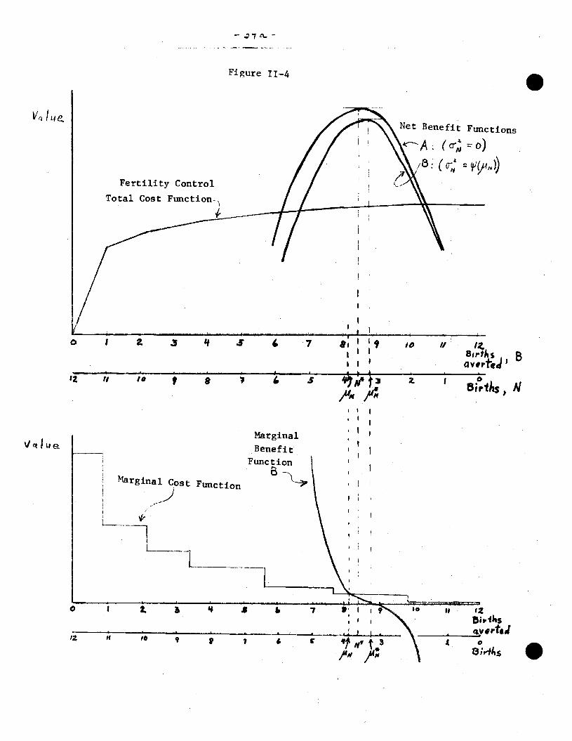
The relationship between these various levels of fertility can be

indicated by coibining figures 11—2 and 11—3 (see figure 11—4). Utility

would be maximized at a level of N N* if the costs of fertility control

were zero and the uncertainty about fertility outcomes were ignored (e.g.

the maximum of the net benefit function A is at a level of N = N*). The

presence of uncertainty modifies the optimum by raising the peak of the

net benefit function (function B) to the level N = . The presence of

fertility control costs further modifies the optimum by lowering the pre—

ferred N to N' the intersection of the marginal cost of fertility control

and the marginal benefit from fertility control.

V IL4

-

Figure 11—4 .

Fertility Control

Net Benefit Functions

o)

(u;; iç14N))

0 I a 3 'I S 7

12 II t 9 4 3II

z I N

Marginal

Benefit

FunctionB-..

Margina' Cost Puj0

I 2.

H

a 7

7 — "1"

II

8i •

— 35 —

III Pure and Mixed Contraceptive Strategies

In the previous section we restricted the discussion of contra-

ceptive strategies to a "pure" strategy defined as one in which the

couple selects some specific contraceptive technique and uses it with

some specific amount of care throughout th reproductive span of T

months. The pure strategy model, in which the couple uses one tech—

nique continuously implies a constant monthly probability of conception

p over the fertile months in the reproductive span. This implication

is essential for the Markov renewal process on which are based the

equations for the mean and varlaftee of fertility outcomes (equations

1 and 2) and the mean—variance curves depicted in figure Il—i. So the

pure strategy model lends itself to a simple analytical structure and

represents a boundary on the relationship between mean and variance of

fertility. As we have noted, this Markov renewal model also underlies

much of the important analytical work done in the past decade in mathe-

matical demography.

However, it is evident that in reality a couple is not restricted

from altering its contraceptive technique over the reproductive span.

Even in the context of a lifetime strategy which could be mapped out

initially and carried out over time, a couple might choose to use dif-

ferent contraceptive techniques (including no contraception) in various

segments of that span of time. Furthermore, since the discussion of the

benefits of fertility control emphasized that under fairly general con—

ditions couples prefer to reduce the variance in their expected fertility,

— 36 —

.it is economically sensible as well as technically feasible for couples

to select a mixed contraceptive strategy which may result in a lower

2aN for any level of expected fertility 1.1

For example, if a couple used the oral contraceptive at its

average observed use—effectiveness throughout its twenty year re-

productive span, Table 11—1 indicates that the distribution of its

expected fertility has a mean of 0.19 births and a variance of 0.18

(point a on the mean—variance curve in figure 11—i). If this couple

wished to have about three children, it could use a less effective

technique or use the pill somewhat carelessly, thereby achieving a

monthly probability of conception of 0.0182 which over a twenty year

span would yield an expected fertility of 3.4 and a variance of 199

(point c on the mean—variance curve in figure lI—i). The couple could

also achieve a mean fertility of 3.4 however by combining periods of

25The economic rationale,offered in Section II, for prefering a

reduced variance in fertility was that any deviation in actual fertilityfrom the desired level of fertility implies a reduction in utility. Thegreater the variance a2 the greater the likelihood that the discrepancybetween actuá3. and desred fertility will be relatively large.

There is an additional economic reason for generally preferring alower variance In the distribution of expected outcomes, risk preferenceaside. The more certain the couple is about the number of children itwill eventually have, the more efficiently it can optimize on the allo—cation of its resources. The couple which is more certain about the timingand number of its children can more efficiently plan its savings pattern,select an optimal size home, automobile, etc., plan the labor force be-havior of the wife, and so forth. The same principles apply here as in

the case of a firm which can achieve lower average cost of production Ifits rate of output is constant over the long run than if its rate of out-put varies significantly from season to season or from year to year.

I

- 37 -

pill use with periods of time in which no contraception was used. The

result would be a mean of 3.4 children and a variance considerably

below that indicated by point c on the mean—variance curve. Indeed the

variance would be no greater than that indicated by point f, the variance

associated with the use of no contractf on over the entire twenty year26

time span.

Furthermore, the pure strategy implies that the births will arrive

at random intervals over the twenty year span, while the mixed strategy

permits the couple to achieve the same number of children with considerable

27control over their spacing. By combining the use of a highly effective

26The logical extreme would be a mixed strategy in which natural

fertility (no contraception)ls pursued in those segments of the repro-ductive span in which a birth is desired and perfect contraception (i.e.

e1 0) at all other times. This strategy would enable a normally fecundcouple to achieve any given number of children fewer than,say, five withvirtual certainty and would also enable them to approximate many plausibledesired spacing patterns fairly closely (see Potter and Sakoda, 1967).

Such a strategy is not only a logical possibility, but it is alsotechnically feasible since the monthly probability may be set to zeroát anytime by reducing coital frequency to zero. The fact that couples do notappear to follow this "perfect contraception" strategy suggests that theproblem of fertility control is not a matter of technical feasibility.The biological constraint on fertility choices must be considered simul-taneously with other constraints on behavior, with fertility goals viewedas competing with other family goals.

27In the pure strategy cse the variance of the interval of time

between successive births, °' is inversely related to p and henceThus, reduction in expected fertility along the mean—variance curve isaccompanied by an increase in the variance

38 —

.technique with periods of no contraception, a couple can achieve its

desired number of children with a relatively low variance and rela-

tively little uncertainty about the spacing of its children.

The mean—variance curve in figure li—i represents the biological

constraint on the distribution of expected fertility when a particular

monthly birth probability persists for the entire span of T months. By

using a mixed strategy, combining contraception with periods of no con-

traception, the biological constraint Is no longer an effective constraint—-

the couple can move off the mean—variance curve toward the horizontal

axis representing a distribution of fertility outcomes of mean and

zero variance. The more efficient the contraceptive technique chosen

during periods of contraception, the smaller is the achievable variance

c2 for any given mean . Thus the more efficient the contraceptiveN

228technique chosen, the weaker is the relationship between

N and

and the smaller is the incentive to lower the mean fertility as a

mechanism for_reducing uncertainty or variance.The mixed strategy (defined in terms of using One specific technique

while contracepting and no contraception otherwise) is feasible only whenthe expected number of births from the continuous use of the technique is

less than the number of children the couple desires. So this form of

Some evidence that the correlation between mean and variance offertility is positive is found in the 1960 !T.S. Census of the Population.Grouping white women married once and husband present into cells definedby husband's occupatIon (8 categories), hushnnd's education (5 categories)and wife's education (3 categories), the unweighted simple correlationbetween and across cells Is 0.89 for women aged 45—54 and 0.77for women aged 35—44. If the younger cohort used better contraceptivemethods on the average, then the reduction in this correlation acrosscohorts is consistent with the implication of a weaker correlation amongusers of better contraception.

S

— 39 —

mixed strategy is more likely to be used the greater is the efficiency of

the contraceptive technique chosen.

In this discussion of mixed strategies of contraception we have

focused upon one particular type of mixed strategy—— that of going on

and going off one contraceptive technique. Although shifting from

contraceptive technique to technique is arther possibility, the theore-

tical discussion of the costs of contraception suggested that this would

not be the case. The fixed costs associated with the adoption of modern

techniques would inhibit technique switching. Consistent with the model's

implication, evidence from the 1965 National Fertility Survey suggests

that technique uwitching has not been a prevalent practice in the U.S.

in the past two decades. Ranking contraceptive methods by their mean

monthly probability of conception (as indicated in Table Il—i) and limiting

the subsample to women who had used some contraception in each of their

first three birth intervals, Nichael (1973) found that the correlation

among techniques used across the three pregnancy intervals was quite

high (ranging from 0.57 to 0.97) for non—Catholic women partitioned by

color and age cohort?9 Ryder and Westoff (1971) study the relationship

29See Michael(1973) Table 4. One note of caution. The NFSdata are oriented by the woman's pregnancy intervals, so Michael hadInformation on only the best technique used by the woman in each in—terval. He could therefore identify switches in contraceptive techniquesfrom pregnancy interval to interval , but not from technique to tech-nique within a given pregnancy interval.

— 41) —

between use and non—use of contraceptionacross intervals and the rela—

tionahip between contraceptive failures in successive intervals. They

find considerable Continuity of contraceptive status across intervals both

in terms of whether a woman does or does not use contraception in succes-

sive intervals and in terms of the degree of success of use across30

intervals.

30

For example, 90% of women who used some contraceptivetechniqueIn the first

pregnancy Interval (from marriage to first pregnancy) useda contraceptive in the second Intervalwhi only 36% of non—users inthe first interval used

a contraceptive in the second interval. Similarpercentages are found for each successivepair of Intervals (i.e. from

the fourth to the fifth intervalthe comparable percentages are 95% and18%). See Ryder and Westoff

(1971), Table IX-19 p. 255. Or, 95% of theWomen who had used contraception in each of the first threepregnancyintervals used contraception in the fourth interval while only 13% ofwomen who had not used contraception

in any of the first three intervalsused contraception in the fourth

(see Ryder and Westoff, (1971) Table IX—23, p. 260).

Evidence of consistency of use across intervals is Indicated by thefollowing rather remarkable statistic: of women who used a contraceptive"sJ1ccessfufly" in the first three

pregnancy intervals, 20% experIencedcontraceptive "failure" in the fourth

pregnancy Interval, while of thosewho had experienced acontraceptive "failure" in each of the first three

intervals, 77% experienced a "failure" again in their fourth interval(see Ryder and Westoff for definitions of success and failure).

This statistic and otherssupport quite strongly, we think, the

contention that couples act as If they adopt a lifetime strategy towardcontraception and that that strategy involves

considerable continuityin the use of a techniquethroughout a lifetime. (The Princeton Studybegun in 1957 also suggested that

across—interval changes in fertilitycontrol are "clearly not a matter of couples shifting from ineffectiveto effective methods " of

contraception. See Westoff, Potter and Sagi1963 (pp. 232—235).)

.

— 41 —

IV Contraception and Fertility Outcomes

In the model described in Section II the household's number of

children, N, is a random variable. The household adopts a contraceptive

strategy which yields a particular value of p, the monthly probability

of conception. Given p as a known and fixed parameter, the household has

an ex ante distribution of fertility characterized by a mean and

variance

The discussion has focused on the ante distribution of fer-

tility outcomes for a single household, but in our empirical analysis

we focus on the corresponding distribution for relatively hoinogenous groups

of households. It is assumed that the observed mean and variance in births

among households with relatively homogeneous demographic—economic charac-

teristics reflect the mean and variance of the distribution of fertility

outcomes faced by each of the households in that group. Recall that

the equation for the variance in number of children (equation 2) assumed

that the unprotected monthly probability of conception and the length

of the period of infertility were constant over the couple's reproductive

lifetime. To apply the model across households implies not only constancy

of these parameters over time for a given household, but also constancy

across households. Heckman and Willis (1973) deal explicitly with the

problem of estimating the average monthly probability p in heterogeneous

groups of households. For our purposes, we will not pursue this issue'

31Consider two populations of fecund, non—pregnant women with identical

mean monthly probabilities of conception, . One population is homogeneousin the sense that p is identical for all members of the population and theother is heterogeneous in the sense that p varies across women according tosome distribution with positive variance. It is known that the mean waiting

time to conception in the heterogeneous population will be longer and the

average birth rate lower than in the homogeneous population, and that thisdifference is a function of the distribution of p in the heterogeneous popu-lation (see, for example, Sheps, 1964).

— tL. —

The model in Section II was set cut in a lifetime context and

considered fertility control in terms of a lifetime strategy. Accordingly,

in our empirical work we frequently use information about contraceptive

behavior at one point in the couple's marriage as an indication or index

of the &ifetime contraceptive strategy. As we indicated in Section III

there is considerable evidence that contraceptive behavior is not charac-

terized by switching from contraceptive technique to technique over the

lifetime. Consequently, in this section we will distinguish couples

either by the best contraceptive technique used lk the time interval

from marriage to their first pregnancy or by the best technique used at any

time In their_marriage. 32

.

32In addition to the evidence cited above

regarding consistencyof technique use between pregnancy intervals, the following tableindicates the percentage of users of a contraceptive techniquein the first Interval who also used that in the secondinterval. The second column Indicates the percentage who used eitherthat same technique or no contraception in the Interval. Thesefigures pertain to white non-Catholic women age 40-44 from the 1965 NFS.

First Interval:% Using % Using Same

Technique Used Same Technique Technique or NoContraception

diaphragm 77% 89%condom 72 82withdrawal 78 85jelly,foatn,

61 67suppository

rhythm 65 85douche 62 73

The table indicates, for example, that of those couples which used thediaphragm in the first pregnancy interval, 77% also used the diaphragmin the second pregnancy interval. Furthermore, of that same group another12% used no contraception in the second pregnancy interval thus a totalof 89% used either that same contraceptive method or no method in thesecond Interval. (The second interval here is defined as either the periodof time from the first to the second pregnancy or from the first pregnaneyto the time of the survey if no second

pregnancy occured.)

Since these data were collected by interview at the time these womenwere 40—44 years of age and pertain to periods of time shortly aftermarriage, there may be a tendency to give the same response for successiveintervals. If so, these percentages overstate the consistency of techniqueselection across intervals.

S

—43—

IIn this and the following section we use the 1965 National

Fertility Survey which was conducted by the Office of Population

33Research at Princeton University. This cross—section survey of some

5600 women aged 55 and under , currently married and living with

their spouse, contains information on the specific contraceptive

technique used in each pregnancy interval, as well as information

on the couple's actual fertility outcome. In this section we use

this data set to document the relationship between contraception use

and fertility outcomes. Since we are interested in studying the

variance in fertility we group the data into cells and study between—

cell differences in observed behavior.

In this section we explore how contraception behavior is re-

lated to the observed disttibution of fertility across groups of

households; we do not attempt to explain ! couples differ in their

desired fertility or in the dispersion of their fertility. Although

we indicated in Section II that the model is capable of treating con-

traception choice and fertility control choice in a simultaneous system

of equations, we do not attempt to estimate the parameters of those

33'1e wish to thank Charles F. Westoff and Norman B. Ryder for

their help in obtaining these data. Our previously published researchfrom this data set (Michael 1973) used a small data file obtained fromProfessor Westoff. Our current research uses the publicly availabledata tape from the 1965 NFS which was acquired through Professor LarryBumpass. The data set is fully described in Ryder and Westoff,duction in the United States 1965, Princeton University Press, 1971.

S

— 44 —

.structura] eluationg. In the tables be&ow, we partition the data set

by household characteristicsincluding color and religion and we use either

the wife's educatf onor expected fertility and either age of wife or marriage

duration to isolate relativelyhomogeneous groups of households. In the

Context of these homogeneousgroups we study contraception strategies as

the mechanism foraffecting fertility outcomes.

Figure IV—1 indicates thefrequency distribution of live births for

women age 35—55 for groups definedby wife's level of schooling, color

and religion. Among the whitenon—Catholics(fjgure IV—la) the distri-

butions appear to be less positively skewed and less dispersed (or more

peaked) among women with higher levels of school1ng4By contrast, the

distributions for nonwhitenon—Catholics (figure IV—lb) are considerably

less peaked and more skewed.Among this latter group the level of

schoolingdoes not distinguish the

frequency distributions so clearly, although

the percentage of households with, say, seven or more births appears to

decline as the level ofschooling rises. Among Catholics (figure IV-lc)

the distributions are somewhatless dispersed than among the nonwhite

non—Catholics, and the level of schoolingdoes not appear to influence

34A few Chi—squared tests have been performed on pairs of distribu-tions of live births for

groups of white non—Catholics with different edu-cation levels from specific S—year cohorts. These tests imply rejection(at a = .05) of the hypothesis that the grade school women's distributionof live births and thecollege women's distribution of live births mighthave been drawn from the same population.

For example, x2 = 36.8 with 12 degrees of freedom for a comparisonof8 years versus. 13 years of schooling for women aged 40—44. The cri-

tical value for x2 with 12 d.f. at a = .01 is 26.2.

S

Frequency3O

Figure 1V—i

Frequency Distribution ofLive Births by Wife's Education,by Color and Religion for

/0

0—8 'iears uItlflhtIIliIittii

9—11 Years........12 Years___113 Years..

0

/0

Is/v

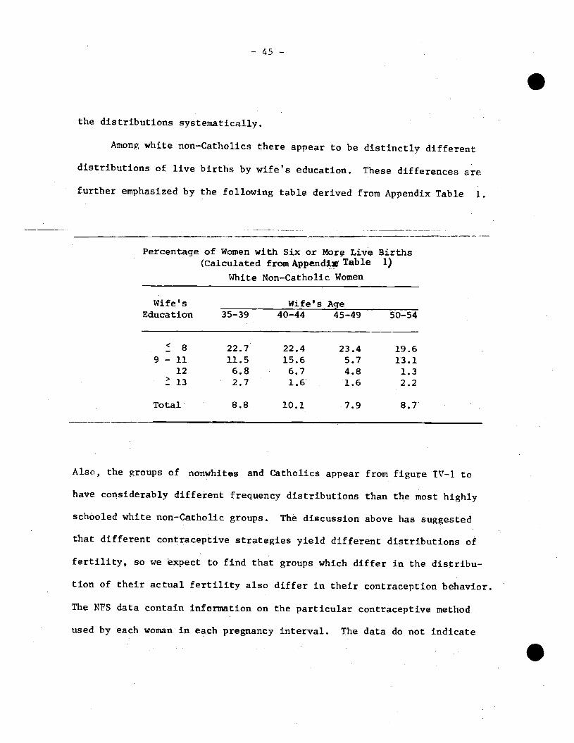
-. 45 —

.the distributions systematically.

Among white non—Catholics there appear to be distinctly different

distributions of live births by wife's education. These differences are

further emphasized by the following table derived from Appendix Table 1.

Percentage of Women with Six or More Live Births(Calculated fromAppend1 Table 1)

White Non—Catholic Women

Wife's Wife'sEducation 35—39 40—44

Age45—49 50—54

8 22.7 22.4 23.4 19.69 — 11 11.5 15.6 5.7 13.1

12 6.8 6.7 4.8 1.313 2.7 1.6 1.6 2.2

Total 8.8 10.1 7.9 8.7

Also, the groups of nonwhites and Catholics appear from figure IV—1 to

have considerably different frequency distributions than the most highly

schooled white non—Catholic groups. The discussion above has suggested

that different contraceptive strategies yield different distributions of

fertility, so we expect to find that groups which differ in the distribu-

tion of their actual fertility also differ In their contraception behavior.

The NFS data contain information on the particular contraceptive method

used by each woman in each pregnancy interval. The data do not indicate

S

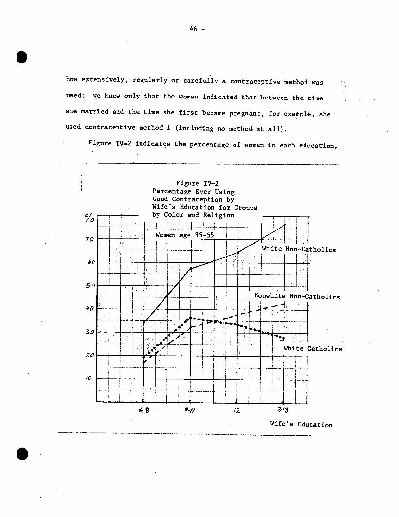
S

— 46 —

how extensively, regularly or carefully a contraceptive method was

used; we know only that the woman indicated that between the time

she married and the time she first became pregnant, for example, she

used contraceptive method I (includin.g no method at all.).

1igure Iv—2 indicates the percentage of women in each education,

S

Figure IV—2Percentage Ever UsingGood Contraception byWife's Education for Groupsby Color and Religion

L_____________ Women age 35—55 _____

— - — — - ______

I

White Catholics

Wife's Education

0//70

50

4'O

30

20

/0

'wi-iiite 1Non—Catholjcs

7

ri .-..—-— ---4---L---

1.u,-1p__1—-.. i.---

Nonwhite Non—Catholics

/

1...;

r

.——i——

—- - - -—'_L____L_.

. —— —— 1 ___T_

- . 4 - L

,

.

,

9-u /2

— 47 — .color and religion group which ever used a "good"35contraceptive technique.

The relationship between these percentages and the distributions of births

indicated in figure IV—1 is striking. Among white non—Catholics, the per-

centage of users of "good" contraceptive techniques rises significantly

with the wife's level of schooling, and this is also the group for which

schooling most clearly distinguishes the distributions of births. The

percentages rise less rapidly by education among the nonwhites, and for

these groups the frequency distributions of births are less clearly de-

lineated by education. Among Catholics neither the percentage of users

of good contraceptive techniques nor the frequency distribution of births

seems to be closely related to wife's education. Thus, in comparisons

among and within color and religion groups, there appears to be a quite con—

sistent relationship: groups characterized by a relatively high percen-

tage of users of good contraception are also characterized by relatively

low dispersion In fertility.

Table TV—i summarizes this same relationship. The table indicates

for each education, color and religion group the percentage of couples

ever using "good" contraception and the actual mean and standard devia-

tion of live births. Groups characterized by a high percentage of users

35Throughout this section, "good" contraception is defined to in-clude pill, IUD, condom and diaphragm. For older cohorts the best a—vailable contraceptive methods were the condom and diaphragm while forthe younger cohorts the more reliable pill and IUD were also available.Since we are attempting at this time to distinguish use of highly re-liable from less reliable techniques, the distinction was arbitrarilymade as indicated. All contraceptive methods other than the pill, TUD,condom and diaphragm are categorized as "poor" methods. The use of nocontraception is called "none" and is distinguished from the "poor"methods.

— 'f/a —

Table I\T—1

Percentage of Couples Using "Good" Contraception,Mean and Standard Deviation of Live Births; by Wife's

Education, Age, Color and Religion

Education_of_Wife8 9—11 12 e 13 Total

White_Non—Catholics

Age 35—44 Z good* 37.4 62.9 67.4 79.9 64.93.658 3.284 2.738 2.583 2.9462.635 1.942 1.567 1.472 1.849(155) (232) (503) (230) (1120)

Age 45—54 % good 29.9 45.4 57.2 67.8 50.9

MN 3.645 2.616 2.136 2.189 2.5792.459 2.004 1.593 1.415 1.962

() (121) (99) (206) (106) (532)

Nonwhite Non—Catholics

Age 35—44 % good 21.7 35.3 41.8 46.9 32.74.968 3.613 3.493 2.531 3.9803.855 3.231 2.636 1.796 3.355

(vt) (124) (119) (67) (32) (342)

Age 45—54 Z good 11.3 21.2 25.0 35.3 17.4

MN 4.474 3.848 1.800 1.765 3.7544.309 3.173 1.765 1.480 3.797

(n) (97) (33) (20) (17) (167)

White Catholics

Age 35—44 % good 18.0 41.6 31.7 28.3 31.6

MN 4.213 3.217 3.353 3.567 3.4672.659 1.831 2.027 2.126 2.111

() (61) (106) (218) (60) (445)

Age 45—54 % good 20.9 23.0 39.3 26.7 28.8

MN 3.646 2.564 2.705 2.133 2.8962.497 1.832 1.395 1.598 1.949

(v') (48) (39) (61) (15) (163)

* percentage of couples in the cell which ever used "good" contraception (i.e.pill, IUD, condom or diaphragm).

** cell size

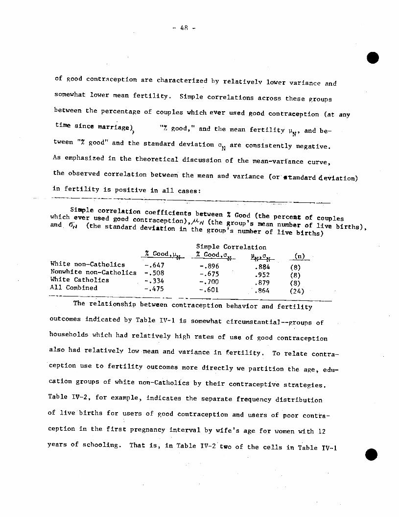
.of good contraception are characterized by relatively lower variance and

somewhat lower mean fertility. Simple correlations across these groups

between the percentage of couples which ever used good contraception (at any

time since marriage) "% good," and the mean fertility N' and be—

tween " good" and the standard deviationare consistently negative.

As emphasized in the theoretical discussion of the mean—variance curve,

the observed correlation between the mean and variance (oratandard deviation)

in fertility is positive in all cases:

Simple correlation coefficientsbetween Z Good (the percent of coupleswhich ever used good

contraceptjon),A (the group's mean number of live births),and G (the standard deviation in the group's number of live births)

Simple Correlation% Good , - % Good ,

White non—Catholics —.647 —.896 .884 (8)Nonwhite non—Catholics —.508 —.675 .952 (8)White Catholics — .334 —.700 .879 (8)All Combined —.475 —.601 .864 (24)

The relationship between contraception behavior and fertility

outcomes indicated by Table IV-1 is somewhat circumstantial——groups of

households which had relatively high rates of use of good contraception

also had relatively low mean and variance in fertility. To relate contra-

ception use to fertility outcomes more directly we partition the age, edii—

cation groups of white non—Catholics by their contraceptive strategies.

Table IV—2, for example, indicates the separate frequency distribution

of live births for users of good contraception and users of poor contra-

ception in the first pregnancy interval by wife's age for women with 12

years of schooling. That is, in Table IV—2 two of the cells in Table TV—i

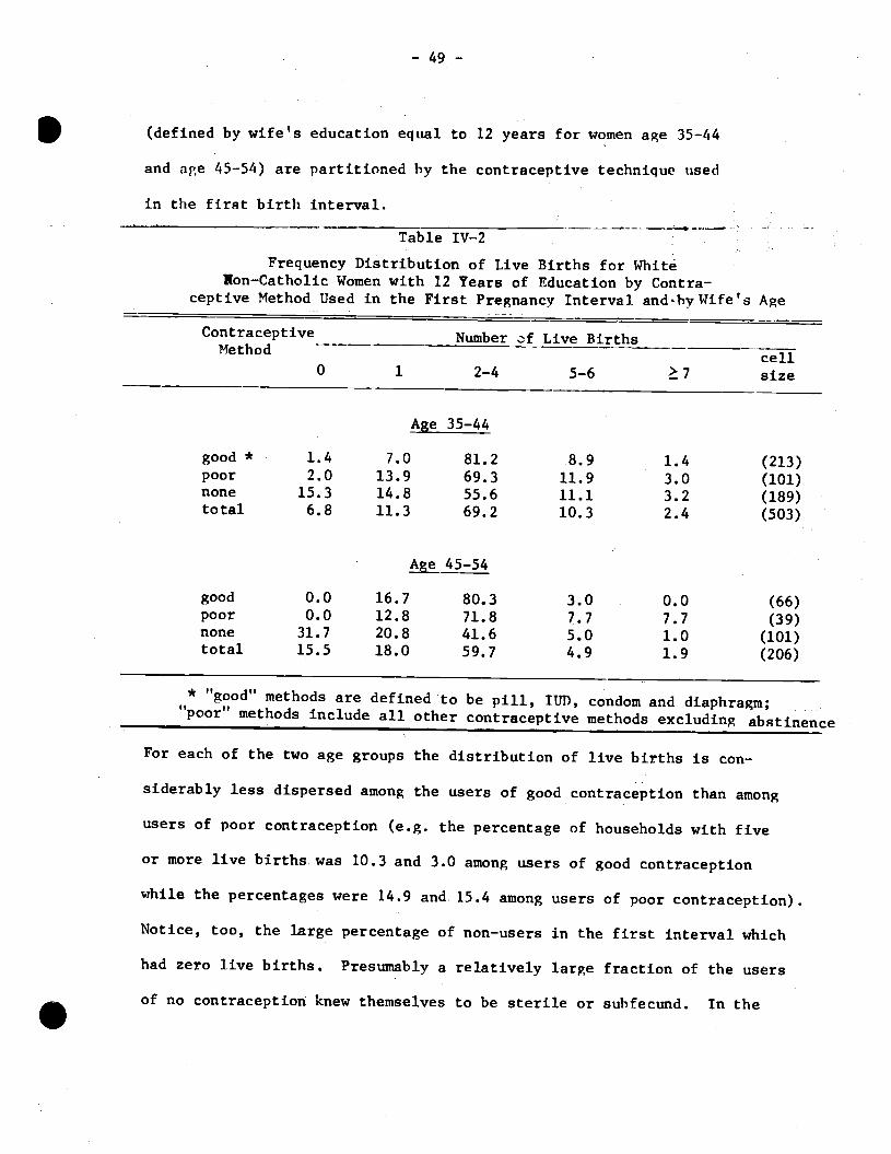
(defined by wife's education equal to 12 years for women age 35—44

and age 45—54) are partitioned by the contraceptive technique used

in the first birth interval.

0 1

— 49 —

Table IV—2

Frequency Distribution of Live Births for WhiteNon—Catholic Women with 12 Years of Education by Contra-

ceptive Method Used in the First Pregnancy Interval. andhy Wife's Age

Contraceptive Number ,f Live Births ________Method2—4 5—6

cell.7 size

Ag 35—44

good * 1.4 7.0 81.2 8.9 1.4 (213)poor 2.0 13.9 69.3 11.9 3.0 (101)none 15.3 14.8 55.6 11.1 3.2 (189)total 6.8 11.3 69.2 10.3 2.4 (503)

45—54

good 0.0 16.7 80.3 3.0 0.0 (66)poor 0.0 12.8 71.8 7.7 7.7 (39)none 31.7 20.8 41.6 5.0 1.0 (101)total 15.5 18.0 59.7 4.9 1.9 (206)

* "good" methods are defined to be pill, 11Th, condom and diaphragm;"poor" methods include all other contraceptive methods excluding abstinence

For each of the two age groups the distribution of live births is con-

siderably less dispersed among the users of good contraception than among

users of poor contraception (e.g. the percentage of households with five

or more live births was 10.3 and 3.0 among users of good contraception

while the percentages were 14.9 and 15.4 among users of poor contraception).

Notice, too, the large percentage of non—users in the first interval which

had zero live births. Presumably a relatively large fraction of the users

of no contraception knew themselves to be sterile or suhfecund. In theS

—50—

.terminology of the model developed in Section II, couples with a rela-

tively low natural fecundity and a low expected fertility need avert

fewer births to achieve any given level of desired fertility. So these

couples have less incentive to use any contraception in general and

less incentive to adopt high fixed cost techniques in particular.

Table IV—3 also indicates the relationship between contraception

use and fertility outcomes. While Table IV—2 shows a frequency dis-

tribution of live births by contraception use for two of the cells of

white non—Catholic women from Table IV—1, Table IV—3 indicates the

mean and standard deviation of the live births by contraception use for

each of the 5 cells of white non—Catholic women age 35—44 from Table IV—1.

Compare the fertility behavior of the "good" and "poor" contra—

ceptors for some given level of schooling in Table IV—3. In terms of

mean fertility, couples which used a "good" contraceptive method pill,

IUD, condom or diaphragm) in the first birth interval had somewhat lower

mean fertility than couples which used relatively "poor" contraceptive

methods. As Panel B indicates, however, very few of the differences in

means are statistically significant. By contrast, the comparison of

differences in the standard deviation of the fertility outcomes does exhibit

statistical significance——the users of poor contraception have appre—

ciably higher variation in their fertility outcomes than do users of

good contraception.36

36Note that in the tests of significance of the variances, thefew pairwise comparisons which were not significant involved the rela-tively small cells containing 40 or fewer observations.

Table IV—3

Mean Nutber of Live Births , p , and Standard Deviation of Numberof Live Births, for White Ln—Catholic Women by Wife's Educationand by the Contraceptive Method (Good, Poor, None) Used in the First

Birth Interval, for Women Aged 35—44

&8 vs.8 vs.

vs.

• ImpliesImp lies

Imp lies

Difference inMeans Variance(t—test) (F—test)1.59 1.95**2.35** 2.63***2.12** 3.67***

statistical difference at astatistical difference at astatistical difference at a

(t—test) (F—test)1.46 1.34**0.92 1.88***0.78 1.40**

(A) .

Contraceptive MethodUsed in First BirthInterval

(Cell Size) 9—11Education of Wife

12 — ?13 Total

p 3.769 3.069Good

N2.065 1.476

() (26) (72)

2.784 2.8871.274 1.076

(213) (124)

2.9201.334

(435)

3.840 3.800Poor 2.444 2.028

(ii) (25) (40)

2.941 2.7061.515 1.488

(101) (34)

3.1851.802

(200)

UN3.587 3.242

None aN 2.817 2.134

(n) (104) (120)

2.577 2.0001.860 1.854

(189) (72)

2.8722.224

(485)

p 3.658 3.284Total

N2.635 1.942

() (155) (232)

2.738 2.5831.567 1.472

(503) (230)

2.9461.849

(1120)

(B)Tests of Statistical Significance of

in Number of Live Births, forDifferences in Means andSpecific Pairs of Cells

Variances

Difference by -_______________Contraceptive Method8 9—11

Education of Wife—12 13

in- -

t—test)—

0.110.450.37

GoodPoorGood

GoodPoorGood

Test of Difference2.03**1.470.64

vs. poorvs. nonevs. none

vs. poorvs. nonevs. none

Means0.911 .82*

1 .20

(Student's0.672.08**3.70***

Tests1.401.331.86**

of Difference1.88**1.112 .09***

in Variance1 .42**

1 .50**

2.14***

(F—test)1 .91***

1 .56

2.97***

Difference byWife's Education

Test of Differences in Mean and Variance of Number of Live Births byWife's Education for Users of Good Contraception Only

9—1112

13

Difference byWife's Education

Difference in

9—119—11

12

Means Variance

vs. 12vs.�. 13vs.2 13

= .10 (two—tailed t—test)..05 (two—tailed t—test).

= .01 (two—tailed t—test).

- 51 -

.The lack of a stronger association between contraception use and

mean fertility in Table IV—3 is somewhat surprising. However, recall

that equation 16 emphasized two opposing forces influencing optimal

mean fertility. The marginal costs of fertility control raised optimal

mean fertility (ik), although the positive relationship between the

mean and variance lowered optimal fertility (—K/2) as a mechanism for

reducing the uncertainty about the number of births. We showed that

couples wishing to avert more births would be induced to adopt better

(higher fixed cost, lower marginal cost) contraceptive techniques. We

also suggested that users of better techniques are more likely to use

a mixed strategy of contraception which implies a weaker relationship

between the mean and variance of fertility. So users of good contra-

ception are expected to have lower marginal costs of fertility control

( a lower ) and also a weaker relationship between mean and variance

C a lower K ). Consequently, if wife's education sorts couples

by their desired fertility in Table IV—3, the further partitioning by

good or poor contraception may not have a systematic effect on mean

fertility. The users of good contraception have lower marginal cost of

averting births, but less incentive to reduce mean fertility as a mechanism

for lowering the uncertainty or variance of fertility. As the relation-

ships in Tables IV—1--—Table IV—3 indicate, across relatively homogeneous

S

—

S groups there is a negative relationship between the use of good con-

traception and mean fertility, but within the homogenous groups,

the use of good contraception systematically affects only the variance of

fertility outcomes. Couples wishing to avert relatively more births have

greater incentives to use good contraception, and within a group homo-

genous with respect to their desired fertility, those who use good contra-

ception achieve a lower variance of fertility.

Table IV—3 also indicates that there is a tendency for the more

educated women to have lower mean fertility and smaller variance of fer-

tility for each contraception category. The differences in the means do

not often exhibit statistical significance (see Panel B), but the differ-

ences in the gariances among users of good contraception are statistical-

ly significant, often at a= .01. The observed relationship between

and across education groups for good and for poor contraception

users separately, mirror the observed relationship between and

across good and poor contraception users holding education constant. This

observation is quite consistent with more educated couples being more

proficient users of each given contraceptive method——the partitioning of

the sample of women aged 35—44 by "good" and "poor' (holding education

constant) yields the same qualitative differences as the partitioning by

more and less education (holding contraception quality constant).

To obtain another measure of the relationship between contraception

choice, the wife's education, and fertility outcomes as indicated in

Table IV — 3, a multiple regression was run using the twelve education—

.

— 53 —

.contraception method cells. Let N1 and V1 he the. mean and standard

deviation of live births in cell j, and P1 be dummy variables re—

flecting the use of good contraception (compared to poor) and poor

contraception (compared to none), and E1 be the wife's education level

(assigned the values 7, 10, 12, and 14 for the respective columns).

The regressions, weighted by the square root of the cell sizes, yielded:

N = 5.23 - 0.18(E )+ 0.34(G ) + 0.42(P )

(8.51) (—3.63 (1.13 (1.43)

and

V = 3.38 - 0.15(E ) - 0.34(G.) - 0.31(P.) .

(15.45) (-8.27' (3.25)1 (-3.03) .1

The wife's education has a significant negative effect on both the

mean and the standard deviation of the number of live births. Con-

traception use had no significant effect on the mean number of live

births, but users of poor contraception had a significantly lower

standard deviation in live births than users of no contraception, and

users of good contraception had a significantly lower standard devia-

tion in live births than users of poor contraception.

Table IV--4 partitions this set of househoiclq , th wh?tp non—(tho—

lics, by duration of marriage and the expected number of children,

for women married only once and aged 35 and above. Since age at mar-

riage differs systematically by several socio-econornic characteristics,

37The standard deviations of N. and V. were 0.559 and 0.517 and

the standard errors of the estimated were .359 and 0.127 respectively.

. T

able

IV-4

Mean Number of Live Births

1"N and Variance in Number of Live Births c2

for White

Non—Catholic Women Aged 3

5 or above and Married Once; by Marriage Durahon, Ex-

pected Number of Children and Contraceptive ethod (Good, Poor, None) Used in the

First Pr

egna

ncy

Inte

rval

Est

imat

ed N

umbe

r of

Bir

ths*

2 3

Tot

al

2 3

4 T

otal

2

3 4

Tot

al

Mar

riag

e D

urat

ion

Mar

riag

e D

urat

ion

Mar

riag

e D

urat

ion

15—

19 Y

ears

20

—24

Yea

rs

25 Y

ears

Goo

d 2.815

3.125

2.907

2.724

2.803

3.455

2.809

2.277

2.842

4.000

2.746

1.162

2.042

1.573

1.349

1.661

4.873

1.745

1.596

1.528

4.286

2.138

(11)

(108

) (88)

(204)

(76)

(61)

(11)

(157)

(47)

(57)

(8)

(114)

Poor

3.300

3.095

3.301

2.952

3.000

3.200

2.946

2.864

3.333

4.636

3.383

2.537

2.283

2.713

1.948

2.455

3.700

2.326

1.933

3.121

6.655

3.464

(n)

(20)

(42)

(73)

(21)

(45)

(5)

(74)

(22)

(48)

(11)

(81)

None

1'N

2.286

3.050

2.640

2.225

3.109

4.333

3.012

1.836

3.106

4.182

3.184

2.790

4.368

4.006

3.512

3.087

5.884

4.182

2.991

5.860

7.466

7.001

(n)

(56)

(101)

(178)

(40)

(92)

(24)

(166)

(55)

(94)

(33)

(201)

Total

2.70

7 3.087

2.866

2.613

2.990

3.950

2.919

2.185

3.085

4.250

3.098

1.881

3.079

2.746

2.107

2.497

5.331

2.867

2.380

3.957

6.623

4.914

(n)

(184

) (2

31)

(455

) (1

37)

(198

) (4

0)

(397

) (1

24)

(199

) (5

2)

(396

)

* E

stim

ated

fr

om a

fer

tility

dem

and

cqua

tion

(see

tex

t fo

otno

te,

p.54

). T

he c

ells

are

def

ined

on

inte

rval

s: 2

is

1.

5 to 2.5; 3 is

2.5

to

3.5,

4 is

3.5 t

o 4.

5.

Tot

al i

nclu

des

obse

rvat

ions

with

est

imat

ed n

umber of births '1.5

and>4.5 as well.

— 54

.the

Partitioning by marriage duration should more adequately standardize

for the length of the period of time at risk of conception. To standard-

ize further for the incentives to avert births, we have used a definition

of expected number of childrenderivé,d by regressing the actual number

of live births on a set ofeconomic and demographic characteristics.38

We used this fertility demandfunction to estimate N for each

household,then grouped households into

cells defined by nterva1s of .One observes in Table IV—4 that when

the marriage duration and

the household's expectedfertility are held constant, users of good

contraception had smaller variation in theiractual fertility than did

users of poor or no contraception.Also, standardized for marriage

duration and contraceptionchoice, households characterized by equal

to three tended to experiencea larger variation in actual fertility than

households characterized by 1 equal to two. That is, there appears

38The regression was estimated from the 1965 NFS for white non—

Catholic women aged 35 or above. The estimation yielded: N = 10.09616— 0.35473 (MARl) — 0.00042 (I) — 0.34462 (ED) + 0.00003 (EDxI) + 0.30078CURB) + 0.09881 (MARD) — O.12119(AGE) where MARl equals 1 if married morethan once or equals zerootherwise; I is an estimate of the husband's in-come at age 40 based on an estimated

earnings function using husband'seducation and market experience; EDis the wife's education level; EDXI

is a multiplicative interactionterm using ED and I; IB equals 1 if thehousehold lives in a rural areaor equals zero otherwise; MARD is theduration of the current

marriage in years; and ACE is the wife's age.39

This procedure partitions the group of households into cells onthe basis of the economic and

demographic chracterjstjcs which, onaverage, are associated with one, two, three or four children. For ourpurposes this procedure suffices, but it does not resolve the problemof partitioning the household's

actual fertility into the "desired" andthe "unwanted" components.

Ito be a positive association between mean fertility and the standard

deviation of fertility. Furthermore, as figure IV—3 indicates, the

positive relationship between and GN appears to be strongest among

users of no contraception.4°

Since more educated women tend to marry at later ages, the total

length of time at risk of conception probably differs by education for

women of a given age. Table IV—3 partitions the sample by wife's age

and education; for comparison Table IV—5 partitions the sample by wife's

education and marriage duration for women married once and aged 35 and

above. Although the cell sizes in Table IV—5 are smaller and the results

somewhat more erratic, one again observes a tendency for users of good

contraception to have somewhat lower mean fertility and, more systematically,

lower variation in their fertility.

The demographic literature has emphasized a distinction between

wanted and "unwanted" fertility, and It is tempting to try to partition

actual fertility into these two components for separate analysis.41

40•The figure plots only cells based on 20 or more observations..

Unfortunately the cell sizes for the users of poor contraception are

quite small, making generalizations difficult.

addition to Ryder and Westoff(1971), see Bumpass and Westoff(1970),Ryder (1973) and Part IV "Unwanted Fertility" of Volume 1 of the Commissionon Population Growth (1972), particularly the essay by Ryder and Westoff (1972).

S

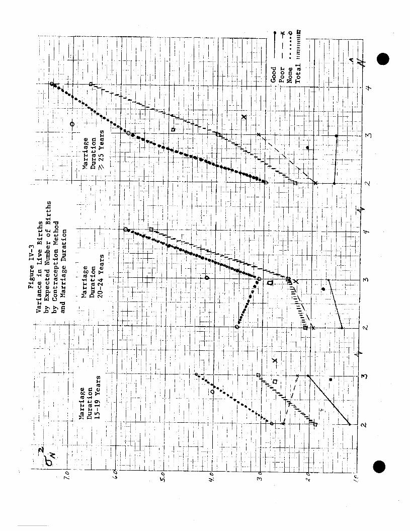
Figu

re IV

—3

- V

aria

nce

In L

ive

Bir

ths

by E

xpec

ted

Nbe

r of

Bir

ths

- -

by C

ontr

acep

tion

Met

hod

____

an

d M

arri

age

Dur

atio

n 70

L

Mar

riage

-H-Marriage

-

Dur

atio

n D

urat

ion

—

15—

19 Y

ears

20

—24

Yea

rs

-

H

H

-

H.

—

- H

H—

- LJ

HIIi

iHiL

L ii:

—

ii

—-

Mar

riage

.

. /

Dur

atio

n .1

—ii:

25 Ye

ars

::I kf

J H

- - --

- -

—-I

I - -a

'---

—--

--i-

- - --

- H

H.

1 - --

. ,4

J-

J1J'

iEH

H /i4

S

.C

3.

2."

—-—

-—

- .

LL

0 —

•0

- --

4-

•0

-- —

.- -

-—-

- H

HtH

ji .F

H--

-—--

__

i___

_I__

_.

4--

- —

- -i-

--

—H

-

- H

jtr I4

-

-

—

4-—

-— -

st

P

7

-. H

HI

4Good

Poor

—

—

X

----

—H

—

4 N

one

--

Tot

al n

ht,I

u,i,J

m

'- --

'-F--

-r

Z4I

H

2

. 3

- #!

: --

t --

I-

- L

- h±t :1

iL

i z

3

2

3 it

S

S

Table IV—5Mean and Standard Deviation of Live Births and Unwanted Birthsfor .Jhite Non—Catholic Women Aged 35 or above and Married Once,

by Marriage Duration, Wife's Education, and Contraceptive Method(Good, Poor, None) Used in the First Pregnancy Interval

(A)

_____ Marriage_Duration_15—19_Years

Contraceptive ducationoUt4IféMethod —

9—11 12 �13 total

Live Births

Good p 3.167 3.192 2.766 3.000 2.907aN 1.722 1.833 1.202 0.984 1.254(i)** (6) (26) (107) (65) (204)

PoorPN 4.182 2.857 3.098 3.429 3.301a 1.991 2.410 1.428 1.453 1.647

() (11) (7) (41) (14) (73)

None ii 2.708 3.146 2.600 2.061 2.640

2.458 2.056 1.946 1.580 2.001

() (24) (41) (80) (33) (178)

TotalPN3.171 3.135 2.768 2.777 2.866

a 2.290 1.988 1.543 1.327 1.657

() (41) (74) (228) (112) (455)

Unwanted Births*

Good p 0.167 0.962 0.523 0.431 0.539

0.408 1.587 1.049 0.770 1.052

(R) (6) (26) (107) (65) (204)

Poor p 2.091 1.714 0.512 0.714 0.904

1.921 2.563 0.952 1.139 1.474

(n) (11) (41) (14) (73)

None p 0.667 1.268 0.837 0.455 0.843

1.341 2.013 1.354 0.905 1.480

() (24) (41) (80) (33) (178)

TotalU.d 0.976 1.203 0.632 0.473 0.716

a 1.573 1.916 1.155 0.859 1.311(R) (41) (74) (228) (112) (455)

* For definition see text** Cell size

— 55c —

Table IV—5

(continued)B

ContraceptiveMethod

Marriage Duration 20—24 Years

Wife—

13 Total-Education

9-11 12of

S8

Live Births

Good

aN(n)

Poor NaN(n)

4.0001.961

(14)

2.0000.926

(8)

2.571 2.784 2.6101.513 1.219 1.115

(28) (74) (41)

3.842 2.686 2.9171.642 1.430 1.379

(19) (35) (12)

2.8091.321

(157)

2.9461.525

(74)

Nonea

()

4.1142.285

(35)

3.366 2.701 1.609

2.009 1.715 1.616

(41) (67) (23)

3.0122.045

(166)

TotaluNa

()

3.7892.169

(57)

3.216 2.733 2.3551.765 1.459 1.402

(88) (176) (76)

2.9191.693

(397)

Gooda

(R)

1.5711.910

(14)

Unwanted Births

0.4330.942

(157)

0.571 0.311 0.1710.920 0.720 0.442

(28) (74) (41)

Poor 'ia1(ii)

0.00.0

(8)

1.211 0.400 0.1671.273 0.604 0.389

(19) (35) (12)

0.5270.879

(74)

None .iU

(R)

1.9712.419

(35)

1.561 0.881 0.3911.988 1.332 1.076

(41) (67) (23)

1.211

1.822

(166)

TotaipcU()

1.5962.203

(57)

1.170 0.545 0.2371.613 1.013 0.690

(88) (176) (76)

0.7761.419

(397)

.

.

Table IV-5

(concluded)

C

ContraceptiveMethod

Education of Wife

9—11 12 113 Total

Live Births

I

S

Good ja1(ti)

3.6881.957

(16)

2.739 2.4711.789 1.065

(23) (51)

2.7081.301

(24)

2.7461.462

(114)

Poor

aN(n)

4.1052.105

(19)

3.400 3.622.113 1.523

(20) (33)

2.6671.658

(9)

3.3831.861

(81)

None

aN(n)

4.2403.004

(75)

3.580 1.9322.548 1.680

(50) (59)

1.7061.359

(17)

3.1842.646

(201)

TotalUNaN(n)

4.1362.724

(110)

3.333 2.4062.295 1.516

(93) (143)

2.3601.439

(50)

3.0982.217

(396)

Good ia11

()

1.0631.843

(16)

Unwanted Births

0.2080.509

(24)

0.4560.961

(114)

0.435 0.3920.896 0.666

(23) (51)

Poor 1.'

GU

(R)

1.0001.291

(19)

0.700 0.8790.979 1.453(20) (33)

0.1110.333(9)

0.7781.235

(81)

Nonea

(R)

1.7332.658

(75)

1.400 0.6442.356 1.283

(50) (59)

0.3530.702

(17)

1.2142.182

(201)

TotalpaU

(R)

1.5092.376

(110)

1.011 0.6081.879 1.157

(93) (143)

0.2400.555

(50)

0.9071.759

(396)

— 56 —

.The difficulty, of course, is in obtaining an estimate of wanted births

distinct from the household's actual fertility. The problem is not sim—

ply one of estimation. Viewed in the rontext of the stochastic model des-

cribed above, it is not possible even in principle to designate each preg-

nancy as !desiredIl or undesired. Also, we have emphasized that the house-

hold's optimal number of children Is affected by fertility control costs

(i.e. In equation 16) and the relation between mean and variance of

fertility (i.e. —K/2). So the definition of "desired" fertility depends

critically upon what is assumed about fertility control costs, the van—42ance in actual fertility, etc.

Recognizing these limitations, we nevertheless attempted to consider

"unwanted" fertility since the NFS data set contains retrospective infor—

mation on the couple's fertility, goals prior to each pregnancy. By summing

42That is, in the terminology of equation 16 one might define un-wanted fertility as — N* or — However, since a > 0, actualfertility N differs in general from N' so "unwanted" fertlity pre-sumably includes not only the discrepancy between some fixed target fer-tility and optimal mean fertility PNbut also the variation in actualfertility around

.

— —

S43

up the number of pregnancies "wanted" and subtracting this number

from the total number of live births, we obtained an estimate of the

number of births "unwanted" in each household. Panel B of Table IV-5

indicates the mean number of "unwanted" births by marriage duration,

wife's education, and contraceptive method used in the first pregnancy

interval. There appears to be a relativeiy strong negative relation

43The NFS data contain retrospective information about the con-

traceptive behavior and the husband's and wife's attitudes about another

pregnancy prior to each of the wife's pregnancies. Following Ryderand Westoff (1971) we considered each live birth as "wanted" or"unwanted" on the basis of the behavioral and attitudinal circumstancesprior to that pregnancy. The birth was considered "wanted" if any ofthe following three conditions was met: (1) The birth was "wanted"if the couple had used no contraception in the interval prior to thatpregnancy and responded "yes" to the question "Was the only reasonyou did not use any method then because you wanted to have a baby as

soon as possible?" (2) The birth was "wanted" if the couple had used

a contraceptive method in the interval prior to that pregnancy and had

"stopped using a method in order to have a child." (3) If the couple wasnot using contraception but responded "no" to the question quotedabove or if the couple had conceived while using a method or while havingstopped using a method but "did not want to become pregnant at that time,"then the couple was asked two additional questions. If the responsewas "yes" to either of these additional questions the birth was con-sidered "wanted." The two questions were "Before you became pregnantthis time did you want to have a (another) child sometime?" and "Didyour husband want to have a (another) child sometime?" Our definition

of"wanted" differs slightly from the definition used by Ryder and Westoff.

.

— 58 —

.between the number of "unwanted" births and the wife's education

44level, and a somewhat systematic relationship between the number

of "unwanted" births and the use of good contraception.

We want to stress that the results pertaining to unwanted

births are subject to many qualifications and are included here pri-

marily as some evidence that this one measure of theintuitively

appealing notion of an unwanted pregnancy seems to be related to

contraception use as one would expect. The arbitrariness of the

precise definition of an unwanted pregnancy helps convince us that it

is more useful in studying the uncertainty related to fertility be-

havior to focus on the distribution of actual births than to concentrate

on partitioning observed fertility into "desired" and "unwanted"

fertility. We have shown in this section that across broadly defined

groups of households there appears to be a systematic relationship

between contraception strategies and the mean and variance of observed

fertility. Couples characterized by the use of more effective contra-

ception appear to have somewhat lower mean fertility, lower variance of

fertility, a weaker relationship between their mean and variance of fer-

tility and perhaps a lower level of "unwanted" fertility.

44This finding is consistent with Ryder and Westoff's conclusion

that "*here is a strong negative association of education and unwantedfertility" (See Ryder and Westoff 1972, p.483). Their conclusion is alsobased on the 1965 NFS data and its sequel, the 1970 NFS, which is not yetavailable to us. It must be stressed however that Ryder and Westoff'sdefinition of "unwanted" pregnancies and their criteria for selection ofthe subsample studied differ from ours and or should not make inferencesabout fertility behavior from comparisons between their tables and ours.

V Diffusion of the Pill

The 1965 National Fertility Study and its sequel, the 1970 National

Fertility Study, provide a unique opportunity to follow, at the household

level, the diffusion of a major technical innovation——the oral contraceptive

——from its Introduction for sale in the TJ.S, in 1960. In addition to the

intrinsic interest of studying the diffusion of new technology, the observed

pattern of adoption of the pill provides an important test of hypotheses

derived from our theory of contraceptive choice (see Section II).

There are two main reasons why the study of pill adoption provides a

more powerful test of our model of contraceptive choice than would he afforded

by studying differential choices among techniques existing before 1960.

First, the introduction of the pill was an exogenous event from the stand-

point of potential adopters. Second, the pill is a truly new kind of con-

traception in comparison with alternative methods available prior to 1960——

it is eignificantly more effective and less coitus—related than alternative

methods. This second consideration suggests that the pill has a significantly

lower marginal cost of fertility control than other methods, at least in terms

of the psychic costs associated with forgone sexual pleasure. Thus couples

were confronted, after 1960, with a significantly different set of potential

contraceptive rethods to choose from, and we investigate in this section the

differential rates of adoption of the pil] aiong women fth different initial

conditions in 1960 (e.g., marital status, age, parity and prior contraceptive

practices).

We first present a few hypotheses about the expected pattern of diffusion

assuming contraceptive choice is governed by factors considered in our theoreti—

S

— 60 — .cal model. Next, we utilize data from the 1965 NFS to test these hy-

potheses and to estimate the probability of pill use as a logistic

function of the household's economic characteristics, parity in 1960, and

prior use of contraception.

The main behavioral hypothesis underlying our theory of choice of

contraceptive technique is that couples choose the least costly tech-

nique to achieve a given fertility goal (e.g. a given value of the mean and

variance of fertility outcomes). It was shown In Section lI—ui that the

same technique will not be least costly for a].l possible goals unless the

technique with the smallest marginal cost Is also the technique with the

lowest fixed cost. This proposition led to the derivation of the contra-

ception cost curve for a "typical" couple in Figure 11—3 as the envelope

of least costly segments of the curve associated with particular contra-

ceptive techniques. According to this analysjs, the more births a couple

expects to avert the more likely it is to choose a technique with rela—

45tively low marginal cost and high fixed cost.

To derive hypotheses about the adoption of the pill from this theory,

we shall assume that for most couples the pill has a lower marginal cost than

other contraceptive techniques available In 1960—65. Since It is easy to

provide examples of components of marginal Cost which are higher for the pill

than for alternative techniques (e.g., money cost, side effects on health,

45For the time being, we shall Ignore risk considerations and argue in terms

of variations in expected fertility within an essentially deterministic frame—work.

S

etc.), the plausibility of this assumption depends on th further

assumption that the major component of the marginal cost of contra-

ception for most people stems from the conflict between effective use

46of a method and sexual pleasure. The fixed cost of the pill includes

the cost of acquiring information about its existence, characteristics

and method of distribution in addition to the money cost of visiting

a doctor to obtain a prescription and various psychic costs (e.g. re-

ligious principles) which are not related to information acquisition.

We can use figure 11—3 (page 31) to il1utrate the hypothetical

fertility control costs faced by a typical couple. Recall that the

line OF2 represents a zero fixed—cost, high marginal cost techniciue such

as withdrawal, and line a F represents another technique such as con-

dom. Suppose that the high fixed—cost, low marginal cost technique

depicted by a4 F4 represents the costs of the pill at the time of its

47introduction on the market in 1960.

46The ITJD, a close rival of the pill in terms of effectiveness and

coitus—related costs, was not widely available until after 1965.

47While the line a F in the figure has a slope, or marginal cost

of approximately zeo the cost curve for the pill could have been drawnwith a positive although relatively low marginal cost.

Also, for simplicity of exposition, we wtll assume here that thesethree techniques, withdrawal, condom, and pill, represent the entire envelopecost curve. In our empirical analysis all available techniqueg are included.

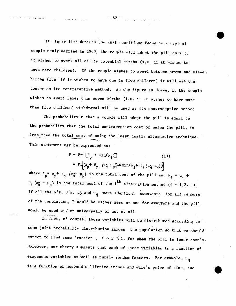
— 62 —

.If ftg(Ir 11—3 dtipiri tht toit tnti1tfon, !v ci

couple newly married in 1960, the couple will adopt the pill only Ifit wishes to avert all of its potential births (i.e if it wishes to

have zero children). If the couple wishes to avert between seven and eleven

births (i.e. if it wishes to have one to five children) it will use the

condom as its contraceptive method. As the figure is drawn, if the couple

wishes to avert fewer than seven births (i.e. if it wishes to have more

than five children) withdrawal will be used as its contraceptive method.

The probability P that a couple will adopt the pill is equal to

the probability that the total contraception cost of using the pill, is

less than the total cost of using the least costly alternative technique.

This statement may be expressed as:

P = Pr EF < Tnin(F1)J (17)

=Pr[@+ , (NUN))m111(al+

where F= a+ (— N) is the total cost of the pill and F = a1+

. — N) is the total cost of the alternative method (1 = 1,2...).If all the a's, s's, and were identical constants for all members

of the population, P would be either zero or one for everjone and the pill

would be used either universally or not at all.

In fact, of course, these variables will be distributed according to

some joint pr?bability distribution across the population so that we should

expect to find some fraction, 0 P 1, for wh. the pill is least costly.

Moreover, our theory suggests that each of these variables is a function of

exogenous variables as well as purely random factors. For example,

is a function of husband's lifetime income and wife's price of time, two

variables hich help determine the couple's demand for children. Like—

wise,ii is a function of the couple's natural fecundahility and the wife's

age at marriage, and the ct's and 's are functions of variables such

as religion and education which determine the fixed and variable costs of

each contraceptive technique.

These considerations suggest that we may express the aggregate

proportion of households using the pfll as

P = fjPr [(F_min(Fj) Ix1,., x)<u] h(x,..., x,u) dx...dxu (18)

where Pr() is the probability of using the pill conditional on the

values of the exogenous variables x1 ,..., x which deteriine natural -.

fertility, the demand for children and the costs of contraception, and

where u is a random variable and h(x,..., x, u) is a joint density func-

tion of the x's and u.

If we ass*nne that u is distributed logistically and is independent

of the x's, the conditional probability of using the pill may be expressed

as a logistic function of the form

P = Ei + exp - (a + h x + ... + bnXn + u (19)

or, alternatively, the natural log of the odds of using the pill becomes a

linear functior. of the form

ln(1) a + bx + u (20)

which can be estimated using standard maximum likelihood procedures.

After discussing several hypotheses about the set of variables x1, x2,...,

X, we estimate the parameters of logistic functions of the form sug-

gested in equation (20).

- 64 -

.We shall first consider the

pattern of pill use in a staticsetting

in which the distributionsof natural fertility,

ii,the demand for children,

and the costs ofcontraception the a's and 5's, are stable in the

Population. Subsequently we consider the question of diffusion of the pill

over time. For convenience,assune for the moment that allcouples In the

population face identical cost functions for the three techniquesdepicted

in figure II-3, but differ in their natural fertility or in their demand

for children. If couplesare then distributed by the number of births they

wish to avert, figure 11-3 implies that the proportion ofcouples in the

population which adopts the pill will be equal to the proportion wishing

to avert 11.5 or more births; theproportion which uses the condom will

be equal to the proportionwishing to avert between seven and 11.5

births,

and the proportion using withdrawal will equal the proportion wishing to a—

vert fewer than seven births. Inshort, given a distribution of couples

by the births they wish toavert, the switching points on the envelope

total cost curve determine theproportion of couples using the various

available techniques.

We have suggested three setsof factors determining the proportion

of couples which might be expected to adopt the pill. We will consider

each in turn. Polding constant factorsaffecting the fertility control

total cost curve (the a's and 8's) and the demand for children (the

any factor which increases natural fertilitywill increase expected births

averted (B Thus for a group of households, an increase in

S

.

— 65 —

d.ll, ceteris paribus, increase the proportion of households using the

48pill (and decrease the proportion using withdrawal). The major observable

variable related to is the wife's age when the pill became available.

So our hypothests is that, ceteris paribus, the older the wife was in

1960 the less likely she is to adopt the pill.49

Alternatively, if we hold constent natural fertility,,u and the

fertility control total cost curve, factors which increase the demand for

children1 reduce the expected averted births B and, therefore reduce the

probability of adopting the pill. In studies of completed fertility,

48In the simple three—techniQue case the effect on condom usage is

uncertain since some who previously used the condom are expected to switchto the pill while some who previously used withdrawal are expected to switchto the condom. In the more general case of several techniques an incressein B is expected to increase the proportion using the high fixed cost, lowmarginal cost technique, ceteris parihus.

That is, the older she is the shorter the remaining reproductivetime span, so the smaller her remaining natural fertility and thus thesmaller her remaining expected averted births. Since she wishes to avertfewer births, ceteris paribus, her incentive to adopt the high—fixed—costpill is relatively slight.

This hypothesis should he qualified in two respects. First, theremay he an advantage to postponing the investment in the fixed cost asso—dated with pill adoption until the benefits of the reduced variable costsassociated with pill use are close at hand. If these benefits are greatestwhen the couple wishes to contracept with high efficiency in order toprevent any additional pregnancy, the adoption of the pill might he post-poned until desired fertility is reached. Second, age at marriage is likelyto be inversely correlated with the couple's demand for children. Sothe younger the woman is at a given parity the more likely she wants tohave a large family, which would tend to offset the effect of age on ex-pected births averted, unless desired fertility is explicitly held constant.Thus our inability to hold desired fertility precisely fixed may introducebiases on the other variables.

— 66 —

.the husband's lifetime income, H, and the wife's education, W,

(as a proxy for her potential lifetime wage or price of time), have

been found to be the most important economic variables. Sanderson

and Willis (1971) and Willis (1973) argued on theoretical grounds for

a positive interaction effect between H and W. Estimating an

equation of the form

p y +y H-VY W+Y 1-lW (21)N 0 1 2 3

in a number of samples of U. S. women, they found that and

are negative and is positive, as expected. If we include these

three variables in the equation for P, since we hypothesize a negative

relationship between N and P, we expect to observe positive coefficients

on H and W and a negative coefficient for

50Briefly, the argument is this. When the wife is not supplying

labor to the market, the shadow price of her time is higher than herpotential market wage and is an increasing function of her husband'sincome. When she supplies labor to the market, her price of time isequal to her market wage and is independent of her husband's income.Since children are assumed to be time-intensive, the positive incomeeffect of H on the demand for children is offset by a substitutioneffect against children in families with non—working wives, whilethere is no offset in families with working wives. Since the wife'slabor force participation is negatively related to H and positivelyrelated to W, Willis (1973) shows that the effects of H andW onnumber of children will be nonlinear with a positive coefficient onthe interaction variable, MW. See, however, Ben Porath (1973) foralternative interpretations of nonlinearity in the demand functionfor children.

51The husband's lifetime income and the wife's education are not,

of course, the only variables relevant for the demand curve forchildren. The demand curve used in the previous section, for example,included several additional variables (see footnote 38 ) and alsopertained to white non-Catholics only. For the analysis of pilladoption in this section we again restrict ourselves to whitenon-Catholics.

.

Estimating the effects on pill use of variation in the fixed

and marginal costs of the pill and alternative methods of contraception

presents a number of difficult problems. These costs are likely to

be dominated by psychic or nontnarket components which may vary widely

across households but cannot be measured directly. Certain variables

such as Catholicism are known to inf1eice the costs of certain forms

of contraception and it is frequently argued that education reduces the

cost of acquiring birth control information (see Michael 1973). Pnfor-

tunately, both of these variables also help determine the demand for

children and it is not easy to see how this influence can be disentangled

from their influence on the cost of contraception.

1

— 68 —

.One advantage of studying the adoption of the pill is the fact

that we may study the response to the introduction of the pill by

women whose initial conditions differed in 1960. This procedure

enables us to study the effect of prior use of other forms of

contraception before 1960 on the probability of adopting the pill

after 1960. The theory suggests that couples which have incurred the

fixed costs associated, with some other technique will, ceteris paribus,

be less likely to adopt the pill. Hence, we expect prior use of the

diaphragm and condom, for example, to be negatively associated with52pill adoption. A second aspect of prior use which may influence the

probability of adopting the pill is the success the couple has with

the previous method. If the couple's previous method has had high

marginal costs, our theory suggests that it would be used relatively

inefficiently. The couple would have, therefore, a higher risk of an

"accidental" pregnancy while using that method. Since the pill has a

relatively low marginal cost, the higher the marginal cost of the

alternative method, the more likely the pill will be adopted.

52That is, after the fixed costs are borne, the fertility controlcosts fall from c1 + to simply B, There are difficulties inthis test of the suruc-cost hypothesis, however. A woman's priorcontraception history is not independent of residual variance caused byvariation in the couple 's demand for children, fecundability, or costsof contraception which we are unable to hold constant with the othervariables in the model. Several potential biases tend to work againstthe "sunk cost" hypothesis. For example, subfecundity or sterility,which may be one of the reasons that a woman has not contraceptod inthe past, would also tend to reduce her probability of adopting the pill.If this bias dominated, we might find that prior users of contraceptionhave a higher rather than a lower probability of using the pill comparedwith prior nonusers.

— 69 —

IConsequently, we expect prior "contraceptive failure" to be positively

related to the probability of adopting the pill. This expectation is

strengthened by the likelihood that couples whic)t have experienced

contraceptive failure confront the prospect of larger losses of

expected utility from additional "unwrted" births than do couples who

have successfully contracepted in the past.

While we have discussed three separate sets of factors influencing

the probability of pill adoption in a static framework, we have not

as yet considered the diffusion of the pill over time. A major driving

force in any process of diffusion of new technology is the reduction

over time of the cost of acquiring information about the new innovation.

By the simple act of adopting and using the new technique, early

adopters convey information to later adopters about the existence of

the technique, how it is distributed, etc. Since the pill is a

prescription drug, its adoption is affected by the diffusion of infor-

mation among doctors as well as among potential adopters. The dynamics

surrounding the cost of information about the pill and the speed and

pattern of its diffusion will also be related to socio-econoaac dif-

ferentials in rates of adoption since this information is spread by

53word of mouth.

53Although they are not information costs, a similar mechanism mayoperate to reduce the costs associated with deviation from group normsas individuals in the group withess increased nonconformity withthese norms. In the case of the pill, the interaction between theteachings of the Catholic Church and the behavior of individual Catholicsmight be interpreted along these lines (see Ryder and Westoff, 1971,Chapter 8).

- 70 — .To consider the effect of decreasing information costs of pill

adoption, we again make use of figure 11-3 (page 31). With the

passage of time the fixed cost (which includes the information cost)

of the pill for the average household may fall from 0c4 to

Thus the switching point--the number of averted births at which pill

adoption is warranted--falls from about 11.5 births averted to about

6 births averted, as the figure is drawn. Obviously, in the aggregate,the reduction in the fixed cost increases the proportion of couples

using the pill. Notice that the model implies that the users of the

next-best technique will be those who most readily adopt the new

technique as its costs of information fall over time. The new low-

marginal-cost technique first displaces the existing technique with

the lowest marginal cost.54

To test the hypotheses advanced above, we have selected three

samples of white non-Catholic women from the 1965 National Fertility

54Hence, should a new contraceptive technique be introduced which

further lowers the marginal cost of contraception, our theory impliesthat the pill could be the first technique to be displaced. Ryder (1972)shows that by 1970 pill use differentials by education, race andreligion had converged. Much of the convergence, however, was causedby an absolute decline in the use of the pill after 1967 by highlyeducated white non-Catholics, the group which has the highest rate ofpill use. It is interesting to speculate whether new techniques suchas the IUD and the increased pepularity of the vasectomy and tuballigation had begun to displace the pill, in this group. Ryder emphasizesthe effects of fears about long—term adverse health effects of the pill,but these alleged effects were not widely publicized until the U. S.Senate hearings in 1969, well after the 1967 peak in pill usage inthe high-use group. .

SStudy who began their first, second or third pregnancy interval in the

period 1960-1964 (see Table V—i for a description of these san1es).

In each sanp1e we estimate the probability that a woman uses the pill

in the specified interval as a function of three sets of variables that

determine, respectively, (1) the womn's potential (i.e. natural) fertility

from the beginning of the interval until menopause; (2) the couple's

demand for children; and (3) the couple's costs of contraception.

These variables, which are listed in Table V—i, may be grouped

as follows:

Variable (Expected Effect on P)

I. Potential. FertilityWife's age in 1965 C—)

II. Demand for ChildrenWife's education (+)Husband's income at age 40 (+)Income-education interaction (-)

III. Cost of Contraception(A) Date interval began (+)(E Used diaphragm in previous interval (-)

Used condom in previous interval (—)Used pill in previous interval (+)Used other method in previous interval C-)

(C) Contraceptive failure in previous interval (+)IV. Age at Marriage (+)

The sign accompanying each variable indicates the hypothesized direction

of effect of that variable on the probability of using the pill in aparticular pregnancy interval. These hypotheses stem from the discussion

on the preceding few pages, and most seem to require no further discussion.

Note that the "date the interval began" operates as a time trend in

I

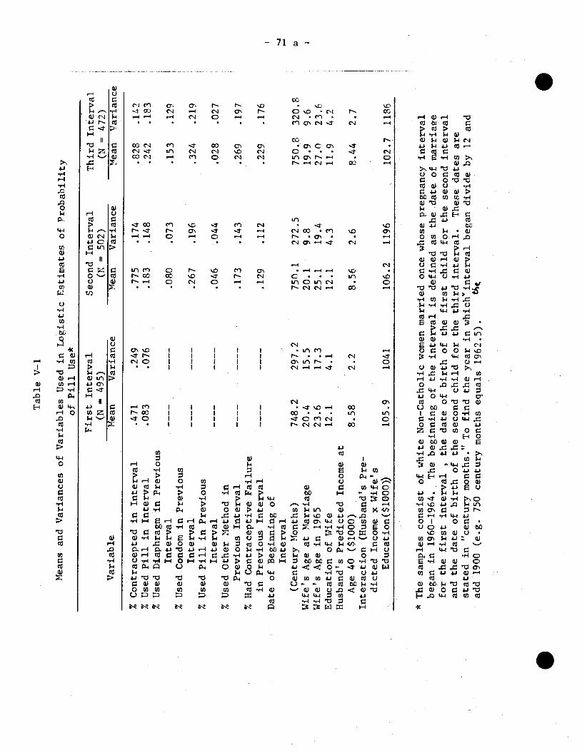
% Contracepted in Interval

% Used Pill in Interval

% Used Diaphragm in Previous

Interval

% Used Condom in Previous

Interval

% Used Pill in Previous

Interval

% Used Other Method in

Previous Interval

% Had Contraceptive Failure

in Previous Interval

Date of Beginning of

Interval

(Century Months)

Wife's Age at Marriage

Wife's Age in 1965

Education of Wife

Husband's Predicted Income at

Age 40 ($1000)

Interaction (Husband's Pre-

dicted Income x Wife's

Education($1000))

Table V—i

S

* T

he samples consist of white Non—Catholic women married once whose pregnancy interval

began in 1960—1964. The beginning of the interval is defined as the date of marriage

for the first interval

, th

e date of birth of the first child for the second interval

and the date of birth of the second child for the third interval. These dates are

stated in "century months." To find the year in which'interval began divide by 12 and

add 1900 (e.g. 750 century months equals 1962.5).

.

Means and Variances of Variables Used in Logistic Estimates of Probability

of Pill Use*

First Interval

Second Interval

Third Interval

(N — 4

95)

Variable

Mean

Variance

(N =

502)

(N = 47

2)

Mean

Variance

Mean Variance

F-

.471

.083

.249

.076

.775

.183

.174

.148

.828

.242

.142

.183

——

——

—

——

—

.080

.073

.153

.129

——

——

—

——

—

.267

.196

.324

.219

——

——

—

——

—

.046

.044

.028

.027

--——

----

.173

.143

.269

.197

——

——

—

——

—

.129

.112

.229

.176

748.

2 20

.4

23.6

12.1

297.

2 15

.5

17.3

4.1

750.

1 20

.1

25.1

12.1

272.

5 9.

8 19.4

4.3

750.

8 19

.9

27.0

11.9

320.

8 9.

6 23.6

4.2

8.58

2.2

8.56

2.6

8.44

2.7

105.9

1041

106.2

1196

102.7 1186

-.1 I-

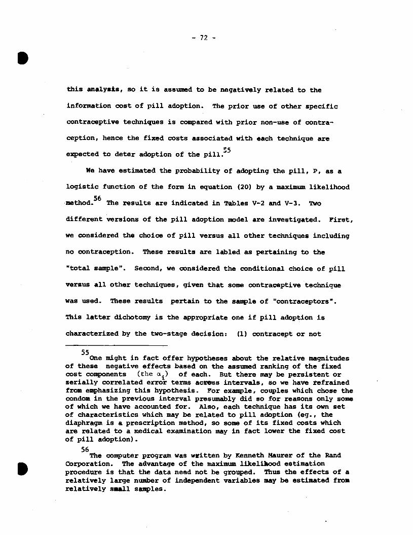
— 72 —

S

this analysis, so it is assumed to be negatively related to the

information cost of pill adoption. The prior use of other specific

contraceptive techniques is compared with prior non—use of contra-

ception, hence the fixed costs associated with each technique are

expected to deter adoption of the pill.'5

We have estimated the probability o adopting the pill, P, as a

logistic function of the form in equation (20) by a maximum likelihood

method.56 The results are indicated in Tables V-2 and V-3. Two

different versions of the pill adoption model are investigated. First,

we considered the choice of pill versus all other techniques including

no contraception. These results are labled as pertaining to the

"total sample". Second, we considered the conditional choice of pill

versus all other techniques, given that some contraceptive technique

was used. These results pertain to the sample of "contraceptors".

This latter dichotomy is the appropriate one if pill adoption is

characterized by the two—stage decision: (1) contracept or not

55One might in fact offer hypotheses about the relative magnitudes

of these negative effects based on the assumed ranking of the fixedcost components (the ct) of each. But there may be persistent orserially correlated error terms across intervals, so we have refrainedfrom emphasizing this hypothesis. For example, couples which chose thecondom in the previous interval presumably did so for reasons only someof which we have accounted for. Also, each technique has its own setof characteristics which may be related to pill adoption (eg., thediaphragm is a prescription method, so some of its fixed costs whichare related to a medical examination may in fact lower the fixed cost

of pill adoption).

56The computer program was written by Kenneth Maurer of the Rand

Corporation. The advantage of the maximum likelihood estimationprocedure is that the data need not be grouped. Thus the effects of arelatively large number of independent variables may be estimated fromrelatively small samples.

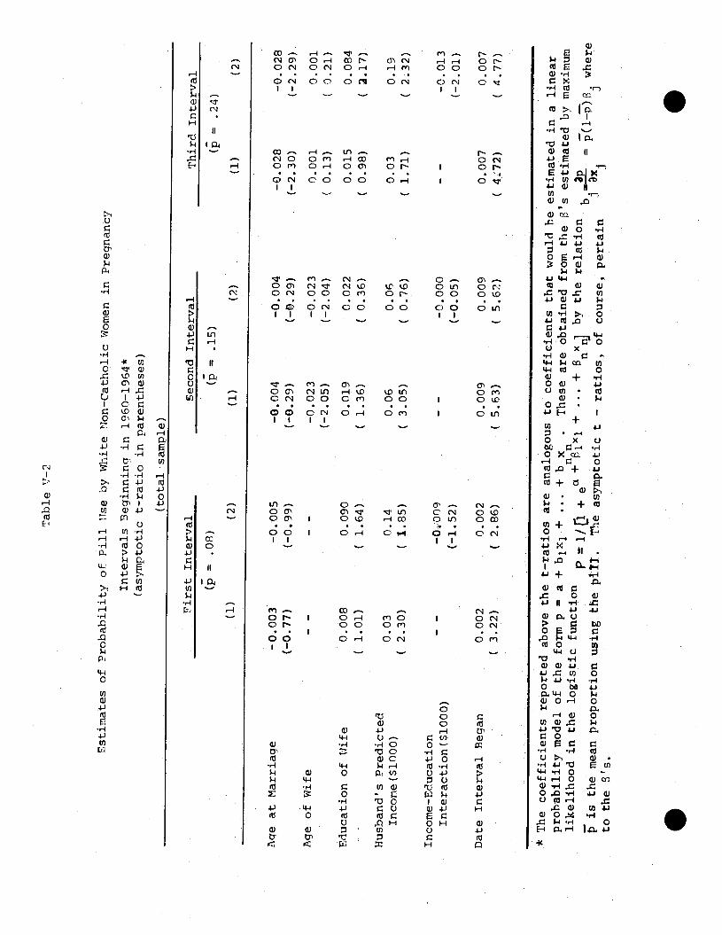
Table V—2

Estimates of Probability of Pill Use by White Uon-Catholic Women in Pregnancy

Intervals Beginning in 1960_1964*

(asymptotic t—ratio in parentheses)

First Interval

Second Interval

Third Interval

(p = .15)

(p

= .08)

(p =

.24)

(1)

(2)

(1)

(2)

. (1)

(2)

Age at Marriage

—0.003

(—0.77)

—0.005

(—0.99)

—0.004

(—0.29)

—0.004

(—p.29)

—0.028

(—2.30)

—0.028

(—2.29) .

Age

of Wife

- —

—

—

—0.023

(—2.05)

—0.023

(—2.04)

0.001

(

0.13

) 0.001

( 0.21)

Education of Wife

0.008

C

1.01

) 0.090

(

1.64

) 0.019

(

1.36

) 0.022

(

0.36

) 0.015

C

0.98

) 0.084

( 2.

17)

Husband's Predicted

Income($1000)

0.03

(

2.30

) 0.14

( 1.

85)

0.06

(

3.05

) 0.06

C 0.

76)

0.03

C

1.71

) 0.19

( 2.

32)

Income—Education

Interaction($1000)

—

—

—0009

(—1.52)

—

—

—0.000

(—0.05)

—

—

—0.013

(—2.01)

Date Interval Began

0.002

3.22)

0.002

(

2.86

) 0.009

(

5.63

) 0.009

(

5.62

) 0.007

(

4.72

) 0.007

(

4.77

)

* The coefficients reported above the t—ratios are analogous to coefficients that would be estimated in a linear

probability model of the form p =

a + b1x1 + ... +

b x

These are obtained from the 's e

stimated by maximum

+ ...

+

x

by the relation

—

—

—

lijel

ihoo

d in

the

log

istic

function P

i/[i +

ea

n b1

=.-

—

p(

l—p)

3. where

is the mean proportion using the pi

ll.

The

asy

mpt

otic

t —

ratio

s, o

f co

urse

, pe

rtai

n to

the

s's

.

. .

Tab

le '1

E

stim

ates

of

Pro

lahi

litv

of 'i

1l T

'se

iw -

Thi

te N

onC

atho

lic '

oren

in

Pren

ancv

Int

erva

ls B

egin

nin2

in

19(—

1)R

t for T

otal

am

nle

and

for

Subs

ampe

of

hon

en w

ho C

ontr

acen

ted

Puri

np the Tnterval*

(asy

mpt

otic

t—

rat i

os i

n pa

rent

hese

s)

Ae

at M

arri

age

Predicted Income of

Husband ($1300)

.050

(2.6)

Income—Education

Interaction ($1000)

Date Interval Began

.009

(5.3

3)

Used Diaphragm in

Previous Interval

Used Condom in

Previous Interval

Used Pill in Previous

Interval

Used Other Method

in Previous Interval

—.119

(1J5)

Contraceptive Failure

in Pr

evio

us I

nter

val

.15

____

__

* S

ee n

ote

at b

otto

m o

f T

able

V—

2 **

Min

imiz

atio

n te

chni

que

did

not

conv

erge

aft

er 1

1

Seco

nd I

nter

val

Thi

rd I

nter

val

—

(3)

(4)

(1)

**

(2)

Age

of

Wif

e

Edu

catio

n of

Wif

e

total sample

çontraceptors

total samole

contraceptors

—.014

—.017

—.024

—.029

(—0.95)

(—0.86)

(—1.92)

(—2.00)

—.015

—.014

.004

.004

(—1.

27)

(_fl

.R9)

(0

.55)

(0

.49)

.0

17

.027

.1

37

.154

(1.15)

(1.29)

(2.07)

(2.07)

— .0

24

(—0.

29)

— .0

89

(—1.

56)

.286

(3.24)

.041

.190

.206

(1.6

6)

(2.2

3)

(2.1

4)

----

-.

013

(—1.

94)

-.01

5 (—

1 .90)

.011

.0

06

.007

(5

.19)

(4

.51)

(4

.25)

- .

077

.076

-.

117

(—0.

75)

(0.9

4)

(—1.

17)

—.1

95

.118

—

.082

(—

2.71

) (1

.74)

(—

0.96

)

.419

.3

70

.228

(2

.P0)

2.

84)

(1.4

1)

—.2

23

.102

—

.095

(?

.70)

(1

.39)

(—

1.04

)

.1'3

.138

.153

(2.5

4)

(2.6

9)

(2.6

2)

.23

.24

.29

142

(2.27)

iterations

— 73 —

.contracept and (2) select a contraceptive technique.

Tab1 V-2 indicates the estimates on the total sample for each

of the first three pregnancy intervals, excluding the variables

which indicate prior contraception use. The time trend (the date

interval began) is positive and statistically significant. This

conforms with our hypothesis regarding the effects of a decline in

information costs over time. The age of the wife has the expected

negative sign in only the second interval, while the age at marriage

has an unexpected negative effect on the probability of pill adoption.58

The effects of the variables related to the demand for children

were computed both with and without the income-education interaction

term. In all cases the variables exhibited the expected signs. The

relatively stronger effect of husband's income than wife's education,

however, is quite surprising. In several studies estimating the effects

of these variables on fertility demand, the wife's education has the

57The estimates were computed on both the total sample (for theunconditional P) and the sample of contraceptors (for the conditionalP). The results were quite similar in the two cases so only the formerare reported here.

58We have no explanation for the consistently negative effect of

age at marriage. }Iolding wife's age and current parity constant, ahigher age at marriage implies a shorter duration of time front marriageto current parity. Thus we think age at marriage in these estimatesmay be positively related to relatively high fecundity, relatively highrates of coital frequency, or relatively low demand for children, buteach of these factors implies a positive effect of age at marriage onthe probability of pill adoption, ceteris paribus.

.

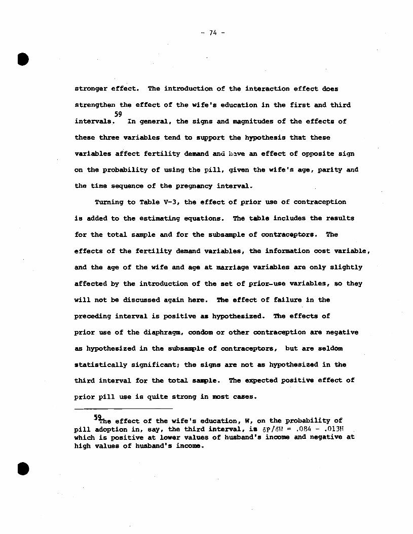
-. 74 —

S

stronger effect. The introduction of the interaction effect does

strengthen the effect of the wife's education in the first and third59

intervals. In general • the signs and magnitudes of the effects of

these three variables tend to support the hypothesis that these

variables affect fertility demand and h2ve an effect of opposite sign

on the probability of using the pill, given the wife's age, parity and

the time sequence of the pregnancy interval.

Turning to Table V-3, the effect of prior use of contraception

is added to the estimating equations. The table includes the results

for the total sample and for the subsample of contraceptors. The

effects of the fertility demand variables, the information cost variable,

and the age of the wife and age at marriage variables are only slightly

affected by the introduction of the set of prior—use variables, so they

will not be discussed again here. The effect of failure in the

preceding interval is positive as hypothesized. The effects of

prior use of the diaphragm, condom or other contraception are negative

as hypothesized in the subsample of contraceptors, but are seldom

statistically significant; the signs are not as hypothesized in the

third interval for the total sample. The expected positive effect of

prior pill use is quite strong in iost cases.

5rhe effect of the wife's education, W, on the probability ofpill adoption in, say, the third interval, is 5p/tSW = .084 — .013Hwhich is positive at lower values of husband's income and negative at

high values of husband's income.

S

— 75 —

.While it is tempting to discuss in detail several of these

estimated coefficients, we will not do so here. We think the

qualitative results of our study of pill use offer rather strong

support for the hypotheses we developed earlier in this section.

In addition, the model can help us interpret the observed trend and,

differential use of the pill since 1960. In the preceding section we

shoved that the implications about the relationship between

distributions of fertility outcomes and Oontraception behavior are

also supported by the observed behavior from the 1965 National

Fertility Survey.

.

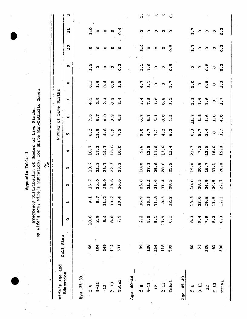
qe 45-49 .

App

endi

x T

able

1

Freq

uenc

y D

istr

ibut

ion

of N

umbe

r of, L

ive

Bir

ths

by W

ife'

s Age, Wife's Education, for White Non-Catholic Women

0/

Ic'

Age 35—39

Wif

e's

Age

an

d E

duca

tion

Cell Size

0

1

Number of Live Births

2

3

4

5

6

7

8

9

10

11

]

8 66

10

.6

9.1

16.7

18

.2

16.7

6.

1 7.

6 4.

5 6.

1 1.

5 0

3.0

9—11

10

4 2.9

8.7

25.0

21.2

17.3

13.5

6.7

2.9

1.9

0

0

0

12

249

8.4

11.2

28

.9.

25.7

14

.1

4.8

4.0

2.4

0.4

0 0

0

13

112

8.0

10.7

28

.6

22.3

18

.8

8.9

0.9

0.9

0.9

0 0

0

Total

531

7.5

10.4

26.6

232

16.0

7.5 43

2.4

1.5

0.2

0

0.4

Age 40—44

9—1].

89

128

2.2

5.5

16.9

13.3

25.8

21.1

18.0

27.3

5.6

12.5

9.0

4.7

6.7

3.1

3.4

7.8

6.7

3.1

1.1

1.6

12

254

5.1

11.8

31.9

25.6

11.8

7.1

5.1

1.6

0

0

13

118

11.9

8.5

31.4

28.8

13.6

4.2

0.8

0.8

0

0

Total

589

6.1

12.2

28.5

25.5

11.4

6.3

4.1

3.1

1.7

0.5

8

60

8.3

13.3

10.0

15.0

21.7

8.3 11.7

3.3

5.0

0

9—11

53

9.4

22.6

28.3

20.8

7.5

5.7

3.8

1.9

0

0

12

126

7.9

19.8

34.9

16.7

13.5

2.4

1.6

1.6

0.8

0.8

13

61

8.2

11.5

29.5

31.1

18.0

0

1.6

0

0

0

Total

300

8.3

17.3

27.7

20.0

15.0

3.7

4.0

1.7

1.3

0.3

0.3

0.3

0 0 0 0.5

1.

( ( (

0 0 0 0 0 0.

1.7

0 0

0

1.7 0 0 0

Frequency Distribution of Number of Live Births

by Wife's Age, Wife's Education, for White Non-Catholic Women

f6

Age 50-54

Wife's Age and

Cel

l. Size

Education

Nber of Live Births

2.

2

3

4

6

7

8

9

10

11

5 3

61

11.5

14.8

8.2

16.4

16.4

13.].

4.9

8.2

9—11

46

6.5

17.4

30.4

21.7

6.5

4.3

8.7

0

4.9

0

0

1.6

0

12

80

27.5

15.0

32.5

15.0

3.8

5.0

1.3

0

0

0

2.2

0

>

13

45

20.0

31.1

22.2

8.9

11.1

4.4

2.2

0

0

0

0

0

0

Total

232

17.7

0

0

2

. .

A-)

Appendix Table 2 a

Frequency Distribution of Best Contraceptive Method Ever Usedby Education for White Non—Catholic Women

Education of Wife _____Method 9—11 12 ' 13 Total

Wife Aged 35—44

Pill 3.2 12.1 10.9 13.0 10.5IUD 0.6 0.4 0.8 1.7 0.9Condom 31.0 35.8 37,4 37.4 36.2Diaphragm 2.6 14.6 18.3 27.8 17.3Withdrawal 8.4 4.7 4.4 1.7 4.5Jelly 3.2 0.9 1.8 2.2 1.9Foam 0.0 0.9 0.4 0.9 0.5Suppository 1.3 0.4 2.0 0.4 1.2Rhythm 3.9 3.9 5.6 2.6 4.4Douche 3.9 7.3 4.0 1.3 4.1Other 0.0 0.0 0.0 0.0 0.0None 41.9 19.0 14.5 10.9 18.5

(n) (155) (232) (503) (230) (1120)

Wife Aged 45—54

Pill 0.0 0.0 2.4 6.6 2.2iui 0.0 0.0 0.5 0.9 0.4Condom 24.0 32.3 32.0 35.8 31.0Diaphragm 5.9 13.1 22.3 24.5 17.3Withdrawal 9.9 9.1 5.3 5.7 7.1Jelly 0.8 2.0 4.8 1.9 2.8Foam 0.0 0.0 0.0 0.0 0.0Suppository 2.5 2.0 0.5 0.0 1.1Rhythm 3.3 3.0 3.4 2.8 3.2Douche 8.3 11.1 1.9 4.7 5.6Other 0.8 0.0 0.0 0.0 0.2None 44.6 27.3 26.7 17.0 28.9

(n) (121) (99) (206) (106) (532)

A-4

Appendix Table 2 b

Frequency Distribution of Best Contraceptive Method Ever Used

by Education for Non—White. Non—Catholic Women

Education ofMethod 8 9-11 12

Wife

>/l3Total

PillIUD

Condom

DiaphragmWithdrawalJellyFoam

SuppositoryRhythmDoucheOtherNone

(n)

2.40.0

18.50.84.04.00.01.60.812.10.039.9

(124)

Wife Aged 35z4

10.90.0

18.55.93.44.21.73.40.88.40.0

42.9

(119)

3.00.0

25.413.46.07.51.54.51.59.00.0

28.4

(67)

9.40.0

21.915.63.16.33.10.06.3

12.50.0

21.9

(32)

6.10.020.26.44.15.01.22.61.510.20.0

42.7

(342)

Wife Aged 45P illIUD

CondomDiaphragmWithdrawal

JellyFoam

SuppositoryRhythmDoucheOtherNone

(n)

0.01.08.22.11.03.10.00.00.019.60.0

64. 9

(97)

3.00.015.23.00.03.03.00.03.0

21.20.048.5

(33)

0.00.0

10.015.00.010.00.05.00.05.00.055.0

(20)

0.00.0

35.30.00.00.00.00.00.011.80.0

52.9

(17)

0.60.6

12.63.60.63.60.60.60.6

17.40.0

59.3

(167)

S

Appendix Table 2c

Frequency Distribution of Best Contraceptive Method Ever Usedby Education for White Catholic Women

— Education_of_Wife ______Method 9—11 12 13 Total

Wife Aged 35—44

Pill 6.6 10.4 5.5 5.0 6.7IUD 0.0 0.0 0.5 1.7 0.4Condom 9.8 25.5 17.4 18.3 18.4Diaphragm 1.6 5.7 8.3 3.3 6.1Withdrawal 21.3 11.3 6.9 5.0 9.7Jelly 3.3 1.9 0.0 3.3 1.3Foam 0.0 0.9 0.0 1.7 0.4Suppository 0.0 1.9 1.4 0.0 1.1Rhythm 13.1 16.0 35.8 38.3 28.3Douche 6.6 0.9 2.3 1.7 2.5Other 0.0 0.0 0.0 0.0 0.0None 37.7 25.5 22.0 21.7 24.9

(n) (61) (106) (218) (60) (445)

Wife Aged 45—54

Pill 0.0 0.0 1.6 0.0 0.6IUD 0.0 0.0 0.0 0.0 0.0Condom 14.6 17.9 27.9 26.7 21.5Diaphragm 6.3 5.1 9.8 0.0 6.7Withdtawal 6.3 15.4 6.6 13.3 9.2Jelly 2.1 0.0 0.0 6.7 1.2Foam 0.0 0.0 0.0 0.0 0.0Suppository 0.0 0.0 0.0 0.0 0.0Rhythm 10.4 15.4 19.7 13.3 15.3Douche 10.4 5.1 3.3 0.0 5.5Other O'..O O.Q 1.6 0.0 0.6None 50.0 41.0 29.5 40.0 39.3

(n) (48) (39) (61) (15) (163)

i.3ihllography

Becker, Gary S., "A Theory of the Allocation of Time," Economic Journal,Vol. 75, September 1965, pp. 493—517.

-

Becker, Gary S. "A Theory of Marriage:Part I,' Journal of PoliticalEconomy, Vol. 81, No. 4, July/August 1973.

Ben—Porath, Yoram, "Economic Analysis of Fertility in Israel: Point andCounterpoint," Journal of Political Economy, Vol. 81, No.2, Part II,March/April 1973, pp. s202—233.

Bumpass, Larry and Charles F. Westoff, "The 'Perfect Contraceptive' Popu—lation," Science, Vol. 169, No. 3951, September 18, 1970, pp. 1177—1182.

Cain, Glen G., "Issues in the Economics of a Population Policy for the

United States," American Economic Review, 61, (May, 1971), pp.4O8—417.

Heckman, James and Robert J. Willis , "Estimation of a Stochastic Model ofReproduction:An Econometric Approach,"NBER Conference on Research inIncome and Wealth, November 1973, mimeo.

Henry, L., "La Feondite' Natureile, Observation, The"orie, Resultats,"Popu—lation 16 , 1961, pp. 27—48 and 261—282.

Jam, A,K., "Predicting Duration—Specific Averages and Variances of LiveBirths: Application of a Stochastic Model of Human Reproduction," 1968Social Statistics Section, Troceedings of the American Statisticalsociation, pp. 248—255.

Keeley, Michael C., "A Model of Marital Formation: The Determinants of theOptimal Age at First Marriage," mimeo, University of Chicago, August 27,1973.

Kelly, Allen C., "Demographic Changes and American Economic Development:Past, Present and Future," U.S. Commission on Population Growth and the

American Future, Economic_Aspects of Population Growth, (ed,) Morss andReed, Vol. II, 1972, Government Printing Office, pp. 9—43.

Keyfitz, Nathan, "How Birth Control Affects Births," Social Biology, June 1971.

Kramer, Marcia, Ph.D. thesis in progress on the demand for legal abortionin New York City, National Bureau of Economic Research, 1973.

Kuznets, Simon, "Population Change and Aggregate Output," Demographic andEconomic Change in Developed Countries, National Bureau of Economic

Research, Princeton University Press, 1960, pp. 324—351.

Lancaster, Kelvin J,, "A New Approach to Consumer Theory," Journal of_PoliticalEconomy, Vol. 74, April 1966, pp. 132—157.

Lindert, Peter H., "The Relative Cost of American Children," Discussion

Paper Series Economic History, The University of Wisconsin, Madison, FH73—18, March 1973.

Michael, Robert T., "Education and the Derived Demand for Children",

S Journal of Political Economy, Vol. 81, No. 2, Part II, March/April1973, pp. 128—164.

Michael, Robert T. and Edward P. Lazear, "On the Shadow Price of Children",presented at the 1971 meetings of the Econometric Society, NewOrleans, Louisiana, December 1971.

Michael, Robert T. and Gary S. Becker, "On the New Theory of ConsumerBehavior", Swedish Journal of Economics, No. 4, 1973 (forthcoming).

Mincer, Jacob, "Market Prices, Opportunity Costs, and Income Effects",in Measurement in Economics: Studies in Mathematical Economics andEconometrics in Memory of Yehuda Cnfe1d, Stanford, 1963.

Mincer, Jacob and Solomon Polachek, "Family Investments in Human Capital:Earnings of Women", Journal of Political Economy, 1974 (forthcoming).

Perrin, Edward and Mmdcl C. Sheps, "Human Reproduction: A StochasticProcess", Biometrics, Vol. 20, March 1964, pp. 28—45.

Potter, R. G., "Births Averted by Contraception: An Approach ThroughRenewal Theory", Theoretical Population Biology, Vol. 1, 1970,pp. 251—272.

Potter, R. G., "Births Averted by Induced Abortion: An Applkcation ofRenewal Theory", Theoretical Population Biology, Vol. 3, 1972,pp. 69-86.

Potter, a. G. and J. M. Sakoda, "Family Planning and Fecundity",Population Studies, Vol. XX, No. 3, 1967, pp. 311-328.

Reed, Ritchie H. and Susan McIntosh, "Cost of Children", U. S. Commissionon Population Growth and the American Future, Economic Aspects ofPopulation Growth, Vol. II, U. S. Government Printing Office, 1972,pp. 333 — 350.

Ryder, Norman B. and Charles F. Westoff, Reproduction in the UnitedStates, 1965, Princeton: Princeton University Press, 1971.

Ryder, Norman B., "Time Series of Pill and IUD Use: United States,1961-1970", Studies in Family Planning, Vol. 3, No. 10, October 1972,The Population Council.

Ryder, Norman B. and Charles F. Westoff, "Wanted and Unwanted Fertilityin the United States: 1965 and 1970", U. S. Commission on PopulationGrowth and the American Future, Demographic and Social Aspects ofPopulation Growth, Vol. I, U. S. Government Printing Office, 1972.

Ryder, Norman B., "Contraceptive Failure in the United States", FamilyPlanning Perspectives, Vol. 5, No. 3, Summer 1973, pp. 133—144.

— il_i —

Sanderson, Warren and Robert J. Willis, "Eoonomic Models of Fertility:Some Examples and Implications", in New Directions in EconomicResearch, National Bureau of Economic Research 51st Annual Report,NBER Inc., September 1971.

Schultz, Theodore W. (ed.), New Economic Approaches to Fertility, NBER,Conference Volume OC #6, 1973 (printed as Journal of Political Economy,Vol. 81, No. 2, Part II, March/April 1973).

Schultz, Theodore W. (ed.), Marriage, Family Human Capital and Fertility,NBER, Conference Volume OC #7, 1974, forthcoming (printed as Journalof Political Economy, Vol. 82, No. 2, Part II, March/April 1974,forthcoming).

Sheps, Minde]. C., "On the Time Required for Conception", Population Studies,Vol. 18, 1964, pp. 85-97.

Sheps, Mindel C. and Edward B. Perrin, "Further Results from a HumanFertility Model with a Variety of Pregnancy Outcomes", Human Biology,Vol. 38, No. 3, September 1966, pp. 180—193.

Taeuber, Irene B., "Growth of the Population of the United States in theTwentieth Century", U. S. Commission on Population Growth and theAmerican Future, Demographic and Social Aspects of Population Growth,Vol. I, U. S. Government Printing Office, 1972, pp. 17-84.

Tietze, Christopher, "The Clinical Effectiveness of Contraceptive Methods",American Journal of Obstetrics and Gynecology, Vol. 78, September 1959,

pp. 650—656.

Tietze, Christopher, "Probability of Pregnancy Resulting from a SingleUnprotected Coitus", Fertility and Sterility, Vol. 11, No. 5, September/October 1960, pp. 485—488.

Tietze, christopher, "The Use-Effectiveness of Contraceptive Methods", inResearch in Family Planning, edited by Clyde V. Kiser, Princeton:Princeton University Press, 1962.

Westoff, Charles F. and Robert Parke, Jr. (eds.), U. S. Commission onPopulation Growth and the American Future, Demographic and SocialAspects of Population Growth, Volume I of Commission Research

Reports, Washington, D.C., U. S. Government Printing Office, 1972.

Willis, Robert J., "A New Approach to the Economic Theory of FertilityBehavior", Journal of Political Economy, Vol. 81, No. 2, Part II,March/April 1973, pp. sl4 - s64.

Willis, Robert J., "The Economic Determinants Of Fertility Behavior",Ph. D. dissertation, University of Washington, 1971. .