nber working paper series stuck on gold: real …
TRANSCRIPT

NBER WORKING PAPER SERIES
STUCK ON GOLD:REAL EXCHANGE RATE VOLATILITY
AND THE RISE AND FALL OF THE GOLD STANDARD
Natalia ChernyshoffDavid S. JacksAlan M. Taylor
Working Paper 11795http://www.nber.org/papers/w11795
NATIONAL BUREAU OF ECONOMIC RESEARCH1050 Massachusetts Avenue
Cambridge, MA 02138November 2005
We thank Paul Bergin, Michael Bordo, Christopher Hanes, John James, Christopher Meissner, MauriceObstfeld, and Kevin O’Rourke for helpful suggestions. The usual disclaimer applies. The views expressedherein are those of the author(s) and do not necessarily reflect the views of the National Bureau of EconomicResearch.
©2005 by Natalia Chernyshoff, David S. Jacks, and Alan M. Taylor. All rights reserved. Short sections oftext, not to exceed two paragraphs, may be quoted without explicit permission provided that full credit,including © notice, is given to the source.

Stuck on Gold: Real Exchange Rate Volatility and the Rise and Fall of the Gold StandardNatalia Chernyshoff, David S. Jacks, and Alan M. TaylorNBER Working Paper No. 11795November 2005 Revised November 2006JEL No. F33, F41, N10
ABSTRACT
Did adoption of the gold standard exacerbate or diminish macroeconomic volatility? Supporters
thought so, critics thought not, and theory offers ambiguous messages. A hard exchange-rate regime
such as the gold standard might limit monetary shocks if it ties the hands of policy makers. But any
decision to forsake exchange-rate flexibility might compromise shock absorption in a world of real
shocks and nominal stickiness. A simple model shows how a lack of flexibility can be discerned in
the transmission of terms of trade shocks. Evidence on the relationship between real exchange rate
volatility and terms of trade volatility from the late nineteenth and early twentieth century exposes
a dramatic change. The classical gold standard did absorb shocks, but the interwar gold standard did
not, and this historical pattern suggests that the interwar gold standard was a poor regime choice.
Natalia [email protected]
David S. [email protected]
Alan M. TaylorDepartment of EconomicsUniversity of CaliforniaOne Shields AvenueDavis, CA 95616and [email protected]

2
Introduction
An assumption of structural change in the macroeconomy stands at the heart of some of the most
influential narratives of the economic history of the early twentieth century. Massive changes in
political economy and macroeconomic policy supposedly derived from an increasing degree of
inflexibility. By the late 1920s these rigidities left economies vulnerable to economic shocks
under a fixed exchange-rate regime. Despite a prevailing gold standard mentalité, democratic
pressures encouraged policymakers to react and experiment with new macroeconomic policies,
provided they could break free of their ideological fetters (Polanyi 1944; Temin 1989;
Eichengreen 1992; Eichengreen and Temin 2000).
Still, evidence for these kinds of structural changes is largely fragmentary and
unsystematic, with samples limited by country or time period, leaving the conventional view
short of support and open to criticism. This paper re-examines the question using a much larger
panel dataset covering both prewar and interwar periods. By indirect identification, we locate a
structural change in open economy macroeconomic dynamics between the classical and interwar
gold standard period.
These questions are of more than antiquarian interest. The optimal choice of an exchange
rate regime remains one of the most durable problems in international macroeconomics. The
essential tradeoff facing policy makers then and now was highlighted by the Mundell-Fleming
model and is central to all New Open Economy Macroeconomic (NOEM) models. On the one
hand, hard pegs can provide the economy with a nominal anchor. On the other hand, a flexible
exchange rate can act as a shock absorber to buffer the economy from external shocks in the
presence of nominal rigidities.
A clear illustration of how stickiness interacts with a fixed-versus-floating choice is
provided in the simple classical model of Reinhart, Rogoff, and Spilimbergo (2003). We extend
this approach and it is one we think quite suited for historical analysis. Indeed, history more
closely resembles this stylized model than does the present. Current debate ranges over the
merits of hard pegs, currency boards, and dollarization at one extreme, via adjustable pegs,
crawling pegs, and dirty floats, to the idealized—even fanciful—notion of the pure float. The
debate is further complicated by the extent to which countries that claim to float actually fix and

3
by the claim that any regime other than the “corner solutions” of hard peg or pure float is
unsustainable.1 Fortunately, the past can more justifiably be reduced to the textbook fixed-
floating dichotomy. Debate over exchange rate regimes a century ago was comparatively simple:
to a first approximation, countries were either on the gold standard or they were floating. To be
sure, there were a few vestiges of bimetallism or silver standards, but the gold standard countries
by 1913 accounted for approximately 48% of countries, 67% of world GDP, and 70% of world
trade.2
Gold had emerged as the dominant monetary regime of its time and as a robust nominal
anchor. Why? The claim was made that it helped to promote international trade and investment,
and the data have since been collected to back it up.3 Small wonder, then, that after the violent
disruptions of World War One the world anchored again to gold in the 1920s. Unfortunately,
despite its past record for stability, the reconstituted gold standard failed; it is now generally
thought to have exacerbated volatility and contributed substantially to the Great Depression
(Kindleberger 1973, Temin 1989, Eichengreen 1992). One measure of this increased instability
that we will study in this paper is the extent of real exchange rate volatility in the world
economy.
Why did an institution that had worked so well for decades become, in the 1920s, “unsafe
for use” (Temin 1989, p. 10)? And what can history teach us about the present?
In this paper we study theoretically and empirically the performance of the gold standard
as a shock absorber, and find that the regime performed very differently at different times. We
show that the classical gold standard did not exacerbate real exchange rate volatility and it coped
well with terms of trade shocks. The interwar gold standard could not handle these shocks very
well, at a time when these shocks turned out to be quite large, and made real exchange rate
volatility worse.
1 On the merits of hard pegs, see, e.g., Calvo and Reinhart (2001) and Dornbusch (2001). On the fragility of pegs seeObstfeld and Rogoff (1995). On the debate over “corner solutions” see Fischer (2001), Frankel (1999). Onmisleading exchange rate regime classifications see Reinhart and Rogoff (2004), Shambaugh (2004), and Levy-Yeyati and Sturzenegger (2005). On why developing countries have a “fear of floating” see Calvo and Reinhart(2002). On flexible exchange rates as shock absorbers see Edwards and Levy-Yeyati (2005).2 Figures derived from Alesina, Spolaore, and Wacziarg (2000), Maddison (1995), and Meissner (2005). On theevolution of exchange rate regimes in the late nineteenth century, and particularly the gold standard, seeEichengreen (1996), Gallarotti (1995), and Meissner (2005).3 On the gold standard and trade see Estevadeordal, Frantz, and Taylor (2003), Flandreau and Maurel (2001), Jacks(2006), and López-Córdova and Meissner (2003). On the gold standard and bond spreads see Bordo and Rockoff(1996) and Obstfeld and Taylor (2003).

4
Conventional Wisdom
As we discuss below, if one wishes to claim that a fixed exchange-rate system such as the gold
standard is an optimal monetary arrangement, one has to invoke an assumption of nominal
(price-wage) flexibility—an assumption that underpins perhaps the most conventional
explanation for why the prewar gold standard worked while the interwar gold standard failed.
It is often argued that nominal flexibility in the world economy was giving way to
increased price and wage rigidity in the early twentieth century. In this view, the gold standard
was compromised as price adjustment shifted from the flexibility assumed by the classical
economists to the stickiness emphasized by the Keynesians. But what evidence can be adduced
in favor of this view? Although it is widely believed, this explanation suffers from a lack of
quantitative support and studies are rare except in a handful of countries. Our cross-country and
cross-regime evidence on shock absorption is a rare attempt at a comparative analysis of this
kind that looks at structural changes in the world economy in many countries both before and
after World War One. We briefly discuss some of the related literature.
Several authors have noted the tendency for nominal rigidities to increase over time in
developed economies, even before the twentieth century. For example, in the United States,
Hanes and James (2003) find no evidence of downward nominal wage rigidity in the mid-
nineteenth century. But there is evidence of some manufacturing wage rigidity beginning in the
late nineteenth century, which appears to have persisted into the twentieth century; this change
may have been related to changes in labor’s bargaining power and was especially strong in firms
that paid high wages, had high capital intensity, or were in highly concentrated industries
(Gordon 1990; Allen 1992; Hanes 1993, 2000). As the structural transformation out of
agriculture and into manufacturing progressed, as capital intensification proceeded in industry,
and as labor’s power expanded, these trends could promote greater stickiness in the economy as
a whole. As long as these nominal rigidities remained minor before 1914, they would have posed
less of a problem for the classical gold standard adjustment than for its interwar successor.
What about evidence from other countries? In a study using panel data for a range of
countries, Basu and Taylor (1999) found a mild increase in the cyclicality of the interwar real
wages, as compared to other historical periods, which is consistent with the Keynesian

5
hypothesis.4 Bordo, Erceg, and Evans (2000) attribute part of the severity of the U.S. Great
Depression to previously absent nominal rigidities. In a study of the U.S., U.K., and Germany,
Bordo, Lane, and Redish (2004) find evidence that deflation was not as damaging before World
War One as in the interwar period, and they suggest that a nearly vertical aggregate supply curve
had become positively sloped by the 1920s as a result of increased nominal rigidities.
Of course, these studies are by no means exhaustive or definitive when it comes to
assessing the evolution of macroeconomic rigidities worldwide and further research is necessary
to assess the heterogeneous experiences of countries. There is also the further problem that data
quality suffers the further back in time we go; for example, the definition of U.S. and U.K.
consumer price indices changes substantially after World War One, an artifact that could bias the
results in the literature. These and other issues still await resolution, and must also be borne in
mind for the present paper.5
Nonetheless, according to the fragmentary evidence we have, it appears that nominal
rigidities were perhaps not entirely absent in the world economy of the late nineteenth century.
But they were on the rise, and almost certainly a factor in the Great Depression where nominal
wages clearly did not fall as rapidly as prices, an observation clearly at odds with the classical
flexible-price model. Indeed, the non-neutral expansionary effect of devaluations in the setting of
the 1930s has been shown for a wide range of countries (Eichengreen and Sachs 1985; Campa
1990; Bernanke and Carey 1996; Obstfeld and Taylor 2004).
An increase in nominal rigidity could offer a reason to expect the interwar period to be
subject to much more turbulent adjustment in the face of shocks. This ought to be manifest in
many of the economy’s vital signs, but our benchmark open-economy macroeconomic models
would suggest that the first place to look for symptoms would be in the behavior of the real
exchange rate. A major goal of this paper is to document empirically the extent to which real
exchange rate behavior shifted as the world economy moved from the classical to the interwar
gold standard. We now present a theoretical structure that informs our empirical design.
4 However, as Hanes (1996) notes, controlling for the long run changes in the composition of the CPI, real wagecyclicality has been quite stable, and long-run comparisons need to allow for the greater countercyclicality of pricemarkups on more finished goods.5 Though not central to this paper, there is also the related question as to whether the rigidities that supposedlycharacterized the interwar period persisted even longer—for the U.S. and U.K., at least, the evidence suggests not(Phillips 1958; Hanes 1996; Huang, Liu, and Phaneuf 2004).

6
Theoretical perspectives
Presently, we develop a simple, static, small open-economy model that extends the analysis in
Reinhart, Rogoff, and Spilimbergo (2003). This classical model is designed to examine the
impact of external shocks on small, open economies and the interaction between nominal rigidity
and the exchange rate regime. The key insight—common to many other models of this sort—is
that nominal rigidity can lead the economy away from its first-best after an external shock, and
policymakers can then employ a change in the nominal exchange rate to improve welfare and
match the hypothetical flexible price equilibrium.
Model
The economy has two sectors. The traded exportable good is a pure endowment good; it is not
consumed at home, but is exchanged for an imported consumption good on world markets
according to exogenously given terms of trade based on world prices denominated in foreign
currency. A nontraded consumption good is produced at home using a single factor,
homogeneous labor; the price of this good and the wage of labor (which are equal) are
denominated in local currency, and they may be sticky. The consumer is a representative agent,
who has preferences over imported goods, nontraded goods, and labor supply. The government
sets the nominal exchange rate; for simplicity, money is not explicitly modeled.
We suppose the economy reaches equilibrium as follows. Home prices and wages are
preset in nominal terms at the start of the period. A terms of trade shock is then observed, for
example, a fall in the foreign-currency price of exports. Under perfectly flexible wages, this
shock will cause internal wages and prices to adjust, and it will turn out that the level of the
nominal exchange rate is immaterial: the exchange rate regime does not matter. Under sticky
wages (of varying degrees) the level of the nominal exchange rate will matter. For example, the
authorities might prefer to engineer a nominal devaluation to offset a decline in the terms of
trade. The optimal degree of devaluation will depend on the characteristics of the utility function,
the degree of nominal rigidity, and the size of the terms of trade shock.
We now make this argument formally. The economy is described by the following
system of equations. The representative consumer has the utility function

7
[ ]43421
444 3444 21
21
1)1(
1
UU
LMCU
−+−+= φρρρ
φαα ,
where C denotes consumption of the nontraded good, M denotes consumption of the imported
good, and L denotes labor supply.6
The consumer’s binding budget constraint is
€
pCC + epM* M = wL + epX
* X ,
where
€
pc is the local-currency price of the consumption good, w is the local-currency wage,
€
pm
*
is the exogenous foreign-currency price of the import good,
€
px* is the exogenous foreign-
currency price of the export good, X is the amount of the export good with which the home
country is exogenously endowed, and e is the nominal exchange rate set by the government.
Competitive constant-returns-to-scale production of the nontraded good takes place using
a labor input with a simple Ricardian technology
LC γ= ,
where
€
γ is an exogenous productivity parameter. The price of the nontraded good is then
€
pC = w /γ , which is true whether prices are sticky or flexible. These properties, plus the budget
constraint, also imply that balanced external trade must hold, since
€
pCC = wL implies
€
epM* M = epX
* X .
The model is solved and applied as follows. Once the world prices of the traded goods
are revealed following a shock, the government makes a choice of e, and then consumers
optimize and achieve some level of utility. Knowing all this beforehand, the government can
attempt to set the optimal level of e to maximize consumer’s utility.
Solution
We now develop the model further so that we can study three cases: perfectly flexible wages,
perfectly sticky wages, and partially sticky wages. (Note that, since prices and wages are
6 Unlike Reinhart, Rogoff, and Spilimbergo (2003), who used a Cobb-Douglas aggregation in the utility component
€
U1, we employ a CES form for greater flexibility and sensitivity analysis.

8
proportional under the competitive Ricardian technology, price stickiness and wage stickiness in
the nontraded sector are one and the same thing here.)
To better understand the solution of model, we can examine the conditions for consumer
maximization based on the Lagrangian
[ ] [ ]XepwLMepCpLMCL XMc**
1 1)1( −−++−−+= λ
φαα φρρρ .
The relevant first order conditions are
[ ] cpCMC λααα ρρρρ =−+ −− 111
)1( , (1)
[ ] *111
)1()1( MepMMC λααα ρρρρ =−−+ −−
, (2)
€
Lφ −1 = λw . (3)
Dividing (1) by (2) and using the fact that
€
pC = w /γ :
€
Cρ = M ρ 1− αα
ρρ −1 pc
epM
*
ρρ −1
= pX* Xp
M
*
ρ1− α
α
ρρ −1 w
epM
* γ
ρρ −1
Let
€
z = w /e denote the local wage measured in foreign currency. The first component of utility
can be written simply as a function of z and exogenous variables and parameters:
[ ]ρ
ρρ
ρρ
ρρρ αγα
αααα
1
1
*
1
*
*1
1 )1(1
)1(
−+
−
=−+=
−−
MMpz
pXp
MCU X
(4)
Further calculations show that the shadow price is given by
€
λ = 1− αep
M
* α 1− αα
ρρ −1 z
pM
* γ
ρρ −1
+ (1− α)
1ρ
−1
Thus, by (3), we find

9
€
U2 = − Lφ
φ= − (λw)
φφ −1
φ= − 1
φz(1− α)p
M
*
φφ −1
α 1− αα
ρρ −1 z
pM
* γ
ρρ −1
+ (1− α)
1ρ
−1
φφ −1
(5)
Adding (4) and (5) we can see that the consumer’s utility
€
U =U(z;...) is a convex
function of one endogenous variable, z, and a host of exogenous parameters and variables. The
optimal level z that attains maximum consumer welfare will be denoted
€
z*, where
),,,,,( *** ρφαγMpXpz X depends on world prices, nontraded productivity, export endowments,
and various parameters. (Of course, in this particular setup, a 1% shock to the endowment of the
export good is isomorphic to a 1% shock to the world price of the export good.)
How does the economy get to
€
z*? If wages are flexible, this is not a problem: the
economy ends up at the first best, as is well known. If wages are sticky, the economy is at a
constrained optimum; yet fortunately, the government can still adjust a flexible exchange rate to
ensure that z attains its optimum value
€
z*, no matter where w is stuck.
The essential intuition is hopefully clear: as in so many models of this type, the welfare-
maximizing planning problem for the authorities is to ensure that the economy replicates the
flexible price equilibrium. Ours is a particularly clean model of this type, with a simple structure
of two sectors, one of which is an endowment sector. However, the intuition will certainly apply
in more general models of the NOEM type.
Three Cases
We apply the model to three cases of interest: perfectly flexible wages, perfectly sticky wages,
and partially sticky wages. We consider the response of the economy with optimal policies to a
standardized decline in the terms of trade, a 1% decline in the price of the export good.
CASE I: In the case of flexible wages, no matter what the level of the exchange rate e, the
local-currency nominal wage adjusts to the first-best level
€
w = z*e. Here, the choice of exchange
rate—and the exchange rate regime—is irrelevant, and welfare is always at the maximum
attainable level. How will the adjustment occur? Because the terms of trade have fallen, the
economy can now afford less of the importable M than before under balanced trade. Relatively
speaking, the consumer must substitute C for M. To be willing to do that, at an optimum, the

10
relative price of the C good must fall, so
€
pC and hence
€
w must fall relative to the local-currency
importable price
€
epM
* . Thus,
€
z* will fall. Suppose
€
d ln z* = ηd ln pX* for some elasticity
€
η. This
says that when the export price falls 1%, the optimal z will fall
€
η%. If e is unchanged, as in a
fixed exchange rate regime, then the fall in w equals
€
η%:
(I: Flexible w; Fixed e,):
€
d lnw = ηd ln pX* ;
€
d lne = 0 .
More generally, even if the authorities adjust e, for reasons unexplored here, it makes no
difference: w takes up the slack, and
€
d lnw = d ln z* + d lne = ηd ln pX* + d lne .
CASE II: In the case of perfectly sticky wages, w cannot adjust at all, and
€
d lnw = 0. So
in this case, if we are to satisfy
€
d ln z* = d lnw − d lne = ηd ln pX* , then the authorities must set
€
d lne = −ηd ln pX* . In the absence of wage flexibility, a flexible exchange rate serves as a shock
absorber in the classic fashion:
(II: Fixed w, flexible e):
€
d lnw = 0;
€
d lne = −ηd ln pX* .
CASE III: The preceding cases are those analyzed by Reinhart, Rogoff, and Spilimbergo
(2003) for the Cobb-Douglas case (where
€
ρ = 0). To extend the analysis to a situation of
partially sticky wages, we now imagine that after any shock hits, domestic local-currency wages
adjust by an amount less than that implied by perfect flexibility, but more than the zero implied
by perfect stickiness. Specifically, suppose wages move by a fraction
€
(1− s) times the amount
they would move under perfect flexibility, so that s (between 0 and 1) is an index of stickiness.
In this case, whatever fraction of the adjustment of z is not met via wage adjustment, remains to
be absorbed by an exchange rate adjustment:
(III: Partial flexibility):
€
d lnw = (1− s)ηd ln pX* ;
€
d lne = −sηd ln pX* .
Clearly, I and II are just special cases of III, when the stickiness parameter takes the
extreme value of 0 or 1. Case III is useful as it allows us to study the response of the economy
under optimal policy when stickiness varies along a continuous range.
Calibration
To explore the implications of the model for optimal exchange rate policy, we simulate the
response to a 1% drop in the world price of the country’s exports. The benchmark parameters are
chosen as follows:
€
w = 1; X = 1; pM* = 1; pX
* = 1; α = 0.5; φ = 1.25; γ = 1; ρ = 0. The latter

11
implies a Cobb-Douglas elasticity of substitution of
€
σ = 1 (where
€
ρ = 1− σ −1). By way of
sensitivity analysis, we also examined the cases
€
σ = 0.5 and
€
σ = 1.5 . The choice of parameters
is justified as follows.
World prices, wages, export endowments, and the nontraded productivity parameter can
be chosen without loss of generality. What about the trade share? Many authors have drawn
attention to the high share of traded output circa 1900 compared with more recent periods (e.g.
Irwin 1996). Thus, although some authors propose higher weights on nontraded goods for
contemporary analysis (sometimes as high as 75%), a weight of 50% on traded goods seems
about right in the gold standard era when tertiary sector activity was much smaller. For example,
a figure of 50% accords with the rough share of “traded” sectors in U.S. GDP circa 1900, where
“traded” is taken to mean agriculture, mining, and manufacturing in the Census Bureau’s (1975)
Historical Statistics. In less advanced economies, the share of nontraded services may have been
even smaller than in the United States.
This leaves two key parameters to be chosen, the parameter
€
φ , which is related to the
labor supply elasticity, and the parameter
€
ρ , which is related to the elasticity of substitution.
Simulation results and inference will be sensitive to these parameters, so careful choices need to
be made. We follow the real business cycle literature and set
€
φ = 1.25, which implies a “high”
labor supply elasticity of 4 (see, e.g. Burstein et al. 2005). In that literature, at least, there seems
to be some consensus on this value.
There is much less consensus on the appropriate parameter value for the elasticity of
substitution in a model of this kind, hence the need for sensitivity analysis. Because this is the
trickiest of out parameter choices, we discuss our choices at some length.
It has proven quite difficult for empirical researchers to pin down with accuracy the
elasticity of substitution, especially at high levels of aggregation. Anderson (1998) states that
“elasticities of substitution are assumed with little empirical foundation. In order to restrict the
response of the nontraded good price in the model, the elasticity of transformation in the base
case is quite high, equal to 5.” Still, there now exist some estimates this high, such as those of
Hummels (1999) as cited by Anderson and van Wincoop (2003), who report that “the average
elasticity is respectively 4.8, 5.6 and 6.9 for 1-digit, 2-digit and 3-digit industries. For further
levels of disaggregation the elasticities could be much higher, with some goods close to perfect
substitutes. It is therefore hard to come up with an appropriate average elasticity.” Anderson and

12
van Wincoop (2003) consider a range of 5 to 10 to be reasonable based on a survey empirical
studies, although again the focus of these studies tends to be on many disaggregated categories of
goods.
One problem for us is that the nontraded-traded distinction is even coarser than the 1-
digit level studied by Hummels. The real elasticity is probably lower. But how low? Some
postulate a very low elasticity of substitution of 0.1; this figure was proposed by Burstein,
Eichenbaum, and Rebelo (2005), but they admit that there is no empirical support for that choice
and it is based on pure introspection. A range of 0.1 to 10 seems hopelessly wide for useful
inference.
Most of the macro literature chooses a value in between. Stockman and Tesar (1995)
calibrated this elasticity at 0.44 based on econometric evidence. Ruhl (2005) notes that the
disagreement between the trade and macro literature poses a problem, but his theory is one that
might explain the lower elasticities used in high-frequency macro analysis. As he sums up:
“International real business cycle … modelers commonly use Armington elasticities around 1.5,
though sensitivity analysis suggests values even lower than this may be appropriate…Not
surprisingly, when empirical researchers have estimated the Armington elasticity from high
frequency data they find small estimates that range from about 0.2 to 3.5.”
The need for sensitivity analysis with respect to the elasticity of substitution is by now
quite obvious. Judging from our survey of the literature, we concluded that 1.5 represents an
upper bound for the parameter in the macro literature, and 0.5 a rough lower bound, at least if we
restrict ourselves to parameters based on the majority of empirical evidence. In between is the
benchmark Cobb-Douglas value of 1.0, the case studied by Reinhart, Rogoff and Spilimbergo
(2003). Thus, we choose values from this range for our sensitivity analysis, focusing on five
discrete choices for the elasticity, namely {0.5, 0.75, 1, 1.25, 1.5}.
Simulations
Since the optimal exchange rate policy is trivial (or immaterial) when wages are perfectly
flexible, Figure 1 (a) examines the more interesting extreme case of perfect stickiness, when
€
s = 1. For the benchmark Cobb-Douglas case (
€
σ = 1) a 1% fall in export prices calls for a 0.34%
optimal nominal depreciation.
13
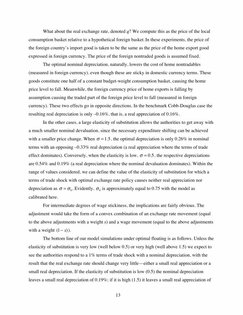
What about the real exchange rate, denoted q? We compute this as the price of the local
consumption basket relative to a hypothetical foreign basket. In these experiments, the price of
the foreign country’s import good is taken to be the same as the price of the home export good
expressed in foreign currency. The price of the foreign nontraded goods is assumed fixed.
The optimal nominal depreciation, naturally, lowers the cost of home nontradables
(measured in foreign currency), even though these are sticky in domestic currency terms. These
goods constitute one half of a constant budget-weight consumption basket, causing the home
price level to fall. Meanwhile, the foreign currency price of home exports is falling by
assumption causing the traded part of the foreign price level to fall (measured in foreign
currency). These two effects go in opposite directions. In the benchmark Cobb-Douglas case the
resulting real depreciation is only –0.16%, that is, a real appreciation of 0.16%.
In the other cases, a large elasticity of substitution allows the authorities to get away with
a much smaller nominal devaluation, since the necessary expenditure shifting can be achieved
with a smaller price change. When
€
σ = 1.5 , the optimal depreciation is only 0.26% in nominal
terms with an opposing –0.33% real depreciation (a real appreciation where the terms of trade
effect dominates). Conversely, when the elasticity is low,
€
σ = 0.5 , the respective depreciations
are 0.54% and 0.19% (a real depreciation where the nominal devaluation dominates). Within the
range of values considered, we can define the value of the elasticity of substitution for which a
terms of trade shock with optimal exchange rate policy causes neither real appreciation nor
depreciation as
€
σ = σ 0. Evidently,
€
σ 0 is approximately equal to 0.75 with the model as
calibrated here.
For intermediate degrees of wage stickiness, the implications are fairly obvious. The
adjustment would take the form of a convex combination of an exchange rate movement (equal
to the above adjustments with a weight s) and a wage movement (equal to the above adjustments
with a weight
€
(1− s)).
The bottom line of our model simulations under optimal floating is as follows. Unless the
elasticity of substitution is very low (well below 0.5) or very high (well above 1.5) we expect to
see the authorities respond to a 1% terms of trade shock with a nominal depreciation, with the
result that the real exchange rate should change very little—either a small real appreciation or a
small real depreciation. If the elasticity of substitution is low (0.5) the nominal depreciation
leaves a small real depreciation of 0.19%; if it is high (1.5) it leaves a small real appreciation of

14
0.33%. In the middle, for the Cobb-Douglas case, the real appreciation is 0.16%. If the elasticity
of substitution is
€
σ 0 (about 0.75) there is no real exchange rate response. For the range of
parameters chosen, the goal of policy, in response to terms of trade shocks, is to smooth them out
using exchange rate policy.
These optimal policy predictions contrast with the outcomes under suboptimal fixed
exchange rates when stickiness is present. In Figure 1 (b), which may be compared with Figure
1(a), we repeat the above exercises but we assume that the authorities are maintaining an
exchange rate peg. Now, of course, in response to each shock to the home export price there is
no nominal devaluation. Thus, the home price level is unchanged: the sticky wage keeps
nontraded prices fixed, and import prices remain fixed because the world price and the exchange
rate do not change. However, the foreign economy still sees its import price decline, causing its
price level to rise by about 0.5%. As a result, the home country always experiences a real
appreciation.
The movements in the real exchange rate are much more volatile in this case than under
optimal floating—compare Figure 1(a) and Figure 1(b). If the elasticity of substitution is low
(0.5) the real appreciation is 0.35%; if it is high (1.5) the real appreciation is 0.60%. In the
middle, for the Cobb-Douglas case, the real appreciation is exactly 0.50%. In absolute size, 1%
fluctuations in the terms of trade cause real exchange rate fluctuations about 50% to 150% times
larger under stickiness and fixed rates than under flexibility or optimal floating.
These general implications are summarized in Figure 2 for a case where we assume that
the elasticity of substitution is close to
€
σ 0 (an assumption we will test). When wages and prices
are flexible, the outcome will always be the same as under the optimal float, that is, a small
response of real exchange rate volatility to terms of trade volatility (the flat line); this response
may even be zero, depending on the elasticity parameter. In contrast, there should be a large
response under a suboptimal peg when wages are sticky (the steep line). When wages are stuck,
the exchange rate must be unstuck to absorb the shock.
Suppose we imagine an experiment in which, all else equal, terms of trade volatility
increases and we observe the change in real exchange rate volatility. Our model shows how
stickiness and the exchange rate regime affect the parameter
€
β in the equation
€
qvol = β × TOTvol (6)

15
where
€
qvol is a measure of real exchange rate volatility and
€
TOTvol is a measure of terms of
trade volatility, and all else is held constant. This is our empirical strategy to identify underlying
structural changes in the economy.
We now arrive at the hypothesis that will be central to the rest of this paper: in a perfectly
flexible economy, there will be no difference between the
€
β measured under fixed and (optimal)
floating rate regimes. But if stickiness is present, this should be detectable in a measurable
change in
€
β under fixed versus floating rates.
To sum up the lessons as we move from theory to empirics: (1) the extent of pass through
from terms of trade shocks to the real exchange rate is an empirical matter (absent knowledge of
deep parameters); but (2) its extent depends on the exchange rate regime only when nominal
rigidities are present.
From Theory to Empirics: Evaluating the Classical and Interwar Gold Standards
The general lessons of this type of model for our historical study are as follows. If prices are
flexible, which we use as a simplifying assumption for the pre-1914 period, then a fixed regime
has few costs. But once prices become stickier, as was supposedly the case in the interwar
period, a different calculus emerges. Then, under a floating rate regime, monetary policy can be
activated to offset an adverse terms-of-trade shock, allowing for some adjustment via nominal
depreciation. The volatility of the real exchange rate will be muted. Under a fixed regime,
however, with nominal rigidities, the same shock will spill over much more into the real
exchange rate. This suggests we follow an empirical strategy that relates real exchange rate
volatility to the monetary regime and the size of the external shocks, and where we also search
for differential impacts of the gold standard on real exchange rate volatility in different eras.
To help guide this strategy we turn to the extant literature on the determinants of real
exchange rate volatility. Rose and Engel (2002) develop a comprehensive framework for
examining the determinants of real exchange rate volatility. They use panel regressions to relate
the volatility of the real exchange rate to independent variables familiar from the gravity model:
“mass” (income and per capita income), monetary measures (nominal exchange rate volatility
and a currency union dummy), and various geopolitical measures (landlocked, common border,
free trade agreement, colonial relationship). Their estimating equations are of the form:

16
€
qvolit = β0i + β0 j + β1evolijt + β2ERregimeijt + γZijt + ε ijt , (7)
where, ijtqvol is the real exchange rate volatility (standard deviation of logged values) for
county-pair i-j; ijtevol is the nominal exchange rate volatility for country-pair i-j;
€
ERregimeijt is
an indicator variable (or a vector of indicators) for the exchange rate regime; and
€
Zijt is a vector
of “gravity” variables.
The literature has also recognized that real exchange rate volatility may, in general,
depend on the size of the nontraded sector in the economy. Thus Hau (2002) uses theory to
explain why one should also include a measure of the trade share (or “trade openness”) of the
economy as an important additional control variable (akin to the trade weight
€
α in our model).
His estimating equation is:
€
qvolit = β0i + β0 j + β1evolijt + β2ERregimeijt + β3(Trade /GDP)ijt + γZijt + ε ijt , (8)
where itGDPTrade / is the average trade share for country pair i-j.
Our model provides two reasons to augment the prevailing approach to estimating
equations such as (7) and (8). A first refinement to these empirical designs is suggested by
equation (6). Our model suggests that the larger the terms of trade shock, the larger is the
necessary adjustment, although this slope should depend on the exchange rate regime and the
degree of wage flexibility (Figure 2). This will turn out to be very important empirically below,
where we estimate variants of a benchmark econometric model of the form
€
qvolit = β0i + β0 j + β1evolijt + β2GSijt + β3(Trade /GDP)ijt + β4TOTvolijt + ε ijt , (9)
where the unit of observation in our data is a non-overlapping 5-year window of annual data for
each pair; ijtGS is an indicator variable for gold standard adherence for country-pair i-j; and
ijtTOTvol is the terms-of-trade volatility (again, standard deviation of logged values) for country-
pair i-j; and i0β and j0β are country fixed effects.
Crucially, we will allow the slope parameter
€
β4 to vary according to the exchange rate
regime (GS), in order to match the qualitative predictions of our model in Figure 2. Hence we set
€
β4 = β40 + β41GSijt , (10)

17
where
€
β40 measures the slope when the country is floating and
€
β41 measures the change in the
slope when the country is on the gold standard. If our model is correct, we expect to see
€
β41 = 0
if the economy is flexible (no difference between the fixed and floating cases) and
€
β41 > 0 if the
economy has nominal rigidities (more volatility under a fixed exchange rate than under optimal
floating).
To sum up, our model suggests that the impact of a gold standard regime will be to raise
the slope parameter
€
β4 under conditions of nominal rigidity. If all other effects are properly
controlled for, we can treat shifts in
€
β4 from one era to the next as evidence of structural
changes. We still need to control for the direct effects of gold standard adherence, nominal
exchange rate volatility, openness and bilateral trade, as per the previous literature (and to avoid
problems of trade endogeneity, we use distance directly as a control variable in OLS estimation).
Data
Our panel dataset comprises quinquennial country-pair observations for a large set of countries
over the period from 1875 to 1939 (e.g., 1875–79, 1880–84, etc.). Throughout, we will estimate
two parallel regressions: the first includes only observations from before 1914 (“prewar”), the
second includes only observations from after 1918 (“postwar”). We omit observations
corresponding to World War One and the German hyperinflation of 1922/23 for obvious reasons.
The data on consumer price indices and annual nominal exchange rates are from the
Global Financial Database, with some corrections by the authors. The set of countries
comprising the sample can be found in Table 1. To construct real and nominal exchange rate
volatilities we followed standard practice: we took the first difference of the log bilateral
exchange rate and then calculated their standard deviations over the five-year windows.
As we can see from Table 2, using either sample, the volatility of both nominal and real
exchange rates changed markedly after World War One. Average real exchange rate volatility
rose from 0.076 to 0.177.7 Its standard deviation also increased from 0.055 to 0.108. Locating the
underlying causes of these changes is a major goal of this paper. We can immediately see that a
7 This change would have been even higher if we included the German data for the 1920–24 quinquennia, the era ofhyperinflation—but we omit this outlying observation.
18
similar pattern is observed for nominal exchange rate volatility, suggesting one possible
explanatory factor.
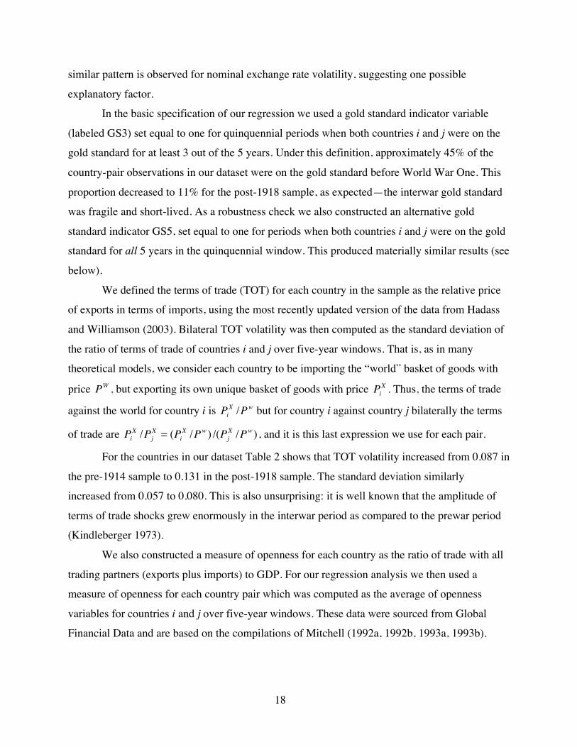
In the basic specification of our regression we used a gold standard indicator variable
(labeled GS3) set equal to one for quinquennial periods when both countries i and j were on the
gold standard for at least 3 out of the 5 years. Under this definition, approximately 45% of the
country-pair observations in our dataset were on the gold standard before World War One. This
proportion decreased to 11% for the post-1918 sample, as expected—the interwar gold standard
was fragile and short-lived. As a robustness check we also constructed an alternative gold
standard indicator GS5, set equal to one for periods when both countries i and j were on the gold
standard for all 5 years in the quinquennial window. This produced materially similar results (see
below).
We defined the terms of trade (TOT) for each country in the sample as the relative price
of exports in terms of imports, using the most recently updated version of the data from Hadass
and Williamson (2003). Bilateral TOT volatility was then computed as the standard deviation of
the ratio of terms of trade of countries i and j over five-year windows. That is, as in many
theoretical models, we consider each country to be importing the “world” basket of goods with
price
€
PW , but exporting its own unique basket of goods with price
€
PiX . Thus, the terms of trade
against the world for country i is
€
PiX /Pw but for country i against country j bilaterally the terms
of trade are
€
PiX /Pj
X = (PiX /Pw ) /(Pj
X /Pw ) , and it is this last expression we use for each pair.
For the countries in our dataset Table 2 shows that TOT volatility increased from 0.087 in
the pre-1914 sample to 0.131 in the post-1918 sample. The standard deviation similarly
increased from 0.057 to 0.080. This is also unsurprising: it is well known that the amplitude of
terms of trade shocks grew enormously in the interwar period as compared to the prewar period
(Kindleberger 1973).
We also constructed a measure of openness for each country as the ratio of trade with all
trading partners (exports plus imports) to GDP. For our regression analysis we then used a
measure of openness for each country pair which was computed as the average of openness
variables for countries i and j over five-year windows. These data were sourced from Global
Financial Data and are based on the compilations of Mitchell (1992a, 1992b, 1993a, 1993b).

19
Results
The dependent variable in all of our regression specifications is the volatility of the real
exchange rate. As a first step we would like to determine whether the gold standard did have a
significant impact on real exchange rate volatility. Our first specification includes the gold
standard indicator variable, nominal exchange rate volatility, and our measures of openness and
distance as independent variables, akin to equation (8). We expect that most of the variation in
the real exchange rate will be attributable to nominal exchange rate volatility. Including nominal
exchange rate volatility as one of our independent variables also allows us to isolate the gold
standard’s auxiliary effect. We are not primarily interested in the effects of the openness and
trade variables, but include them in all of our specifications as control variables.
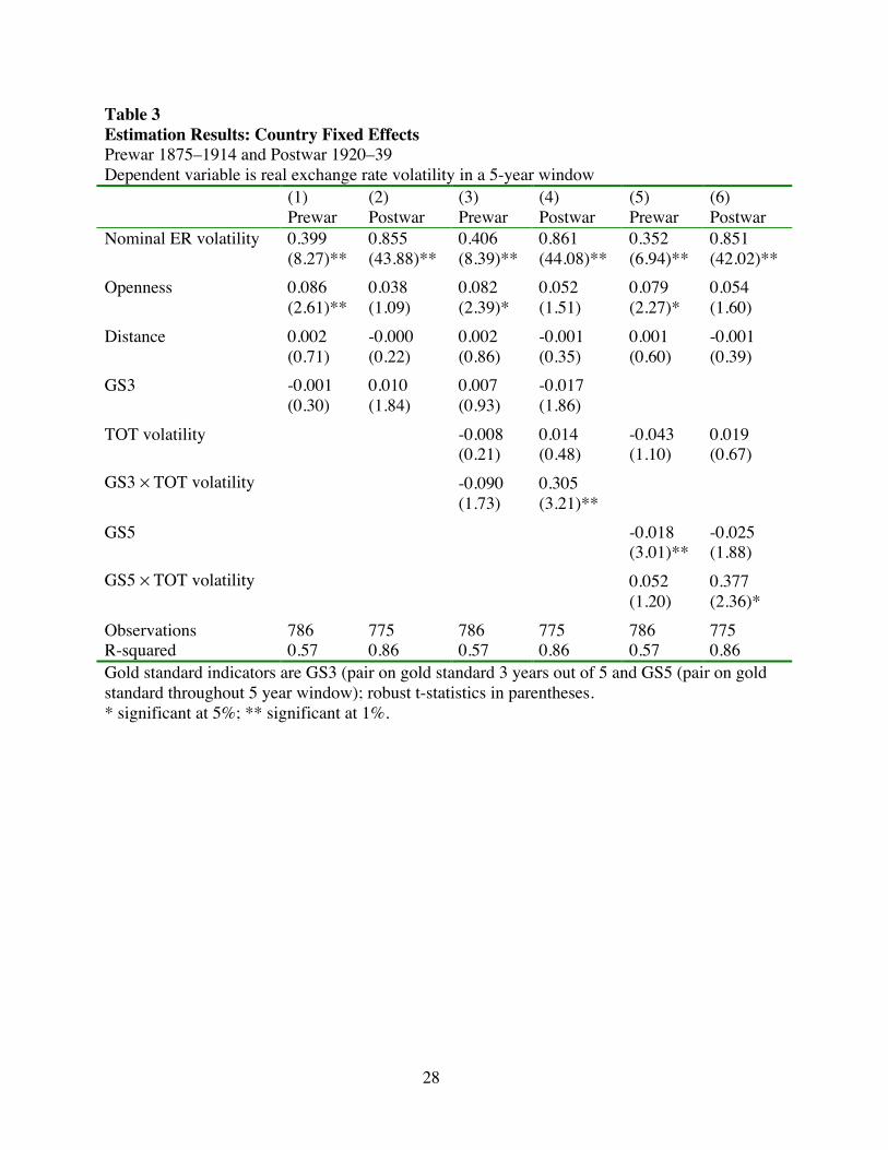
Following the Rose and Engel (2002) country-fixed effects (CFE) specification of
equation (7), the results of our initial specification are reported in the first two columns of Table
3. Including the country fixed effects, this specification captures 86% of the variation for the
post-1918 period, and 57% of the variation for the pre-1914 period. As expected, in both the pre-
1914 and post-1918 regressions nominal exchange rate volatility explains much of the variation
in real exchange rate volatility: the coefficients on the nominal exchange rate are positive and
significant. The estimated coefficient for pre-1914 sample is 0.399, and rises to 0.855 in the post-
1918 sample. In these regressions we find no separate impact of the gold standard on real
exchange rate volatility (that is, independent of its impact on reduced nominal exchange rate
volatility, which was substantial).
However, equations (9) and (10) lead us to suspect that TOT volatility should also be
included as a determinant of real exchange rate volatility. In order to test this hypothesis we
include our measure of TOT volatility and an interaction term between the gold standard
indicator (GS3 or GS5) and TOT volatility as independent variables. Using the GS3 indicator,
the coefficient on terms of trade volatility is negative and insignificant (using a standard 5%
level of significance threshold) for both the pre-1914 and post-1918 sample. The coefficient on
the interaction term for the gold standard and TOT volatility is insignificant for the pre-1914
sample (–0.090); but it is positive and significant for the post-1918 sample (0.305). Higher TOT
volatility was associated with higher RER volatility—but only in the interwar years, and only for
countries on gold.

20
The results in columns 5 and 6 using the GS5 indicator are broadly similar; the
interaction term is 0.052 and insignificant prewar, and is 0.377 and significant postwar.
However, we find here (column 5) that on its own, joining the gold standard was associated with
some discrete reduction in RER volatility, all else equal: the coefficient on GS5 in the prewar
sample is –0.018 (about 1/3 of a standard deviation of the dependent variable) and significant at
the 1% level. It is –0.025 (about 1/4 of a standard deviation of the dependent variable) and
significant at the 6% level in the postwar sample. This dampening effect of the gold standard was
in addition to its effect on nominal exchange rate volatility (which is already controlled for). One
theory for this dampening effect of the gold standard is that, in addition to quelling nominal
exchange rate volatility and promoting trade, the gold standard probably gave further stimulation
to market integration that is not captured in a linear model (Estevadeordal, Frantz, and Taylor
2003; Flandreau and Maurel 2005; Jacks 2006; López-Córdova and Meissner, 2003). This effect
was most likely to be seen in countries that were credibly and durably pegged to gold, an effect
more likely to show up when we use GS5 than when we use GS3, and more likely to be detected
in the larger prewar sample.
Robustness Check
As a further check on the robustness of our results, we re-estimate all of the specifications in
Table 3 but this time using country-pair fixed effects (CPFE) estimation. The logic behind CFE
estimation is that bilateral real exchange rate volatility may be affected systematically by (time-
invariant) country level attributes not captured in the right-hand side variables, but which can be
captured in a full set of country dummies. However, the omitted variable problem may be more
serious if there are also unobservable (time-invariant) pair-specific characteristics that affect real
exchange rate volatility. In that case, the safest way to proceed is by including a full range of
country-pair dummies.
These results are shown in Table 4. They are quite similar to the results in Table 3. The
only material differences appear in columns 5 and 6 using the alternate (and more stringent) gold
standard indicator GS5. In Table 4, the coefficients on GS5 are somewhat larger than in Table 3
(–0.023 prewar and –0.042 postwar in Table 4 versus –0.018 prewar and –0.025 postwar in
Table 3), and the coefficient on GS5–TOT volatility interaction almost doubles in size (0.656 in

21
Table 4 versus 0.377 in Table 3) while its significance level falls from 5% to 1%. Nonetheless, in
what follows we focus on the GS3 coefficients in columns 3 and 4 of Table 4, for two reasons.
First, the GS3 results are more conservative (i.e., have smaller coefficients); second, the number
of observations with GS5 equal to one in the interwar period is very small (28), so we may have
more confidence in estimates based on the more abundant nonzero observations of the GS3
indicator (88).
To sum up, according to our preferred results (Table 4, columns 3 and 4), TOT volatility
has no statistically significant effect on RER volatility before 1914. But after 1914, an increase
in TOT volatility increased RER volatility (with a passthrough coefficient of 0.367), but only for
countries on the gold standard. These differences between the two epochs are highlighted
graphically in Figure 3, which shows predicted values for RER volatility as a function of TOT
volatility based on our preferred results for the four regimes: prewar versus post, and on gold
versus off.
Comparison with the Model
What do these results tell us? First, absent any reliable estimates of the elasticity of substitution
from the literature, we can always use the model to identify this parameter. Recall that if the
elasticity of substitution is close to
€
σ 0 (about 0.75) then there is no real exchange rate response
in our model under flexible wages, or under sticky wages with optimal exchange rate policy (cf.
Figures 1). The flat response of the real exchange rate to terms of trade shocks under both prewar
and interwar floating regimes provides prima facie evidence in favor of a model with an
elasticity of substitution set close to
€
σ 0 , justifying our earlier assumption that this was the
case—in particular, when we were laying out the qualitative story in Figure 2.
The similarity of Figure 3 to Figure 2 is striking. Floats in both eras absorbed shocks
well, as the model would have predicted. As for pegging, the gold standard also absorbed shocks
very well prior to 1914, but the interwar gold standard was a poor shock absorber: increases in
terms of trade volatility resulted in increases in real exchange rate volatility. In our model, as we
saw in Figure 2, this kind of steep response is only seen in one case: fixed regimes with
stickiness. This is the central result of our paper and is consistent with the oft-repeated—but

22
hitherto unsubstantiated—conventional view that the prewar global economy was sufficiently
flexible to cope well with a fixed exchange rate regime, but the interwar gold standard was not.
Our paper documents the rising importance of exchange rate flexibility as a shock
absorber in the early twentieth century, a new finding that underscores the tensions highlighted
by the trilemma-inspired account of the political economy of international finance (Obstfeld,
Shambaugh, and Taylor 2005). Before 1914 the classical gold standard operated by the rules in
an environment in which nominal flexibility, albeit not perfectly fluid, was sufficient to allow the
classical adjustment mechanism to work through price levels alone. In contrast, by the 1920s and
1930s adopting a peg proved costly in terms of enhanced real exchange rate volatility. With
flexibility apparently lost elsewhere in the macroeconomic system, the role of the exchange rate
as a shock absorber suddenly became very important. This is, we believe, the first systematic,
cross-country, and cross-regime study to document this development.
Conclusion: From Unfettered Wages to Golden Fetters?
One of the unifying themes in global macroeconomic history concerns the shift in the adjustment
process in the early twentieth century. It is widely believed that nominal rigidities increased,
setting the stage for the Great Depression and the Keynesian revolution. But what is rare in the
literature is systematic cross-country and cross-regime evidence, using consistent methods to
evaluate the magnitude of these supposed changes. To help fill the gap we use theory to develop
a new diagnostic test that can be applied to panel data from a large sample of countries.
Changes in nominal rigidity can have implications for optimal monetary policy, as can be
seen in a simple classical model (or in more complex models). In the presence of external terms-
of-trade shocks, these rigidities drive a small open economy away from its first-best. For
plausible parameters (at least based on current calibration practices) these same rigidities also
raise the volatility of the real exchange rate, providing us with an indirect test for the changing
strength of such rigidities. The implied diagnostic test: did the ability of the gold standard to
absorb terms-of-trade volatility worsen significantly between the prewar period and the interwar
period as measured by real exchange rate volatility? Our comparative evidence, summarized in
Figure 3, suggests that it did.

23
Two caveats must be offered. First, our model is an important guide, but is a
simplification, as are all economic models. That said, we believe the intuition will survive in
many other models too. The basic point is robust. If an economy is fully flexible, there is no link
between real and monetary outcomes, and the exchange rate regime should make no difference at
all. Thus, even absent any specific model, the key results in Figure 3 present a puzzle to be
explained with respect to one important real linkage—the pass through of terms of trade shocks
into real exchange rate shocks. The exchange rate regime seemed to make no difference before
the war, but it did make a difference after the war. Why? Which parameters changed? Whatever
models other scholars bring to the study of these data, this is a puzzle that must be confronted.
Second, given the limitations of a simple model and panel econometrics, our findings
should not be interpreted as a monocausal explanation of the failure of the interwar gold
standard. The economic—and political—story is much more complex than that (Eichengreen
1992). Country experiences varied greatly, and this will not be captured in our panel coefficient
estimates. Still, as argued by Temin (1989), a rigorous account requires attention to both impulse
and propagation effects; he drew special attention to the major impulse given by the shock of
World War One and its aftermath, which disturbed exchange parities and the global allocation of
gold reserves. Our work draws attention to a potentially important change in the propagation
mechanism. Before 1914, it seems the world economy had enough flexibility that it could ride
out terms of trade shocks even on a hard peg, so that the benefits of shifting to a floating rate
regime were rather small. By the 1920s, this kind of flexibility was in decline just as terms of
trade volatility was on the rise—an unfortunate combination that surely played some part in a
crisis that brought to end the world’s most durable fixed exchange rate regime.

24
References
Alesina, Alberto, Enrico Spolaore, and Romain Wacziarg. 2000. Economic Integration andPolitical Disintegration. American Economic Review 90(5): 1276–96.
Allen, Steven G. 1992. Changes in the Cyclical Sensitivity of Wages in the United States1891–1987. American Economic Review 82(1): 122–40.
Anderson, James E. 1998. Trade Restrictiveness Benchmarks. Economic Journal 108(449):1111–25.
Anderson, James E., and Eric van Wincoop, 2003. Gravity with Gravitas: A Solution to theBorder Puzzle. American Economic Review 93(1): 170–192.
Basu, Susanto, and Alan M. Taylor. 1999. Business Cycles in International HistoricalPerspective. Journal of Economic Perspectives 13(2): 45–68.
Bernanke, Ben S., and Kevin Carey. 1996. Nominal Wage Stickiness and Aggregate Supply inthe Great Depression. Quarterly Journal of Economics 111 (August): 853–83.
Bloomfield, Arthur I. 1959. Monetary Policy under the International Gold Standard:1880–1914. New York: Federal Reserve Bank of New York.
Bordo, Michael D., Christopher J. Erceg, and Charles L. Evans. 2000. Money, Sticky Wages,and the Great Depression. American Economic Review 90(5): 1447–63.
Bordo, Michael D., John Landon Lane, and Angela Redish. 2004. Good versus Bad Deflation:Lessons from the Gold Standard Era. NBER Working Papers 10329.
Bordo, Michael D., and Hugh Rockoff. 1996. The Gold Standard as a “Good Housekeeping Sealof Approval.” Journal of Economic History 56(2): 389–428.
Broda, Christian. 2001. Coping with Terms-of-Trade Shocks: Pegs versus Floats. AmericanEconomic Review 91(2): 376–80.
Burstein, Ariel, Martin Eichenbaum, and Sergio Rebelo. 2005. Large Devaluations and the RealExchange Rate. Journal of Political Economy 113(4): 742–84.
Calvo, Guillermo A., and Carmen M. Reinhart. 2001. Fixing for Your Life. In Susan Collins andDani Rodrik, eds., Brookings Trade Forum 2000. Washington, D.C.: BrookingsInstitution.
Calvo, Guillermo A., and Carmen M. Reinhart. 2002. Fear of Floating. Quarterly Journal ofEconomics 117(2): 379–408.
Campa, José M. 1990. Exchange Rates and Economic Recovery in the 1930s: An Extension toLatin America. Journal of Economic History 50 (September): 677–82.
Dornbusch, Rudi. 2001. Fewer Monies, Better Monies. American Economic Review 91(2):238–42.
Edwards, Sebastian, Eduardo Levy-Yeyati. 2005. Flexible Exchange Rates as Shock Absorbers.European Economic Review 49(8): 2079–2105.
Eichengreen, Barry. 1992. Golden Fetters, New York: Oxford University Press.Eichengreen, Barry. 1996. Globalizing Capital: A History of the International Monetary System,
Princeton: Princeton University Press.Eichengreen, Barry, and Peter Temin. 2000. “The Gold Standard and the Great Depression.”
Contemporary European History 9: 183–207.Estevadeordal, Antoni, Brian Frantz, and Alan M. Taylor. 2003. The Rise And Fall Of World
Trade, 1870–1939. Quarterly Journal of Economics 118(2): 359–407Fischer, Stanley. 2001. Exchange Rate Regimes: Is the Bipolar View Correct? Journal of
Economic Perspectives 15(2): 3–24.

25
Flandreau, Marc, and Mathilde Maurel. 2005. Monetary Union, Trade Integration, and BusinessCycles in 19th Century Europe. Open Economies Review 16(2): 135–152.
Frankel, Jeffrey A. 1999. No Single Currency Regime is Right for All Countries or At All Times.Princeton University International Finance Section. Essays in International Finance 215.
Gordon, Robert J. 1990. What is New-Keynesian Economics? Journal of Economic Literature28(3): 1115–71.
Gallarotti, Guilio M. 1995. The Anatomy of an International Monetary Regime The ClassicalGold Standard 1880–1914. Oxford: Oxford University Press.
Hadass, Yael S., and Jeffrey G. Williamson. 2003. Terms of Trade Shocks and EconomicPerformance 1870–1940: Prebisch and Singer Revisited. Economic Development andCultural Change 51(3): 629–56.
Hanes, Christopher. 1993. The Development of Nominal Wage Rigidity in the Late 19thCentury. American Economic Review 83(4): 732–56.
Hanes, Christopher. 1996. Changes in the Cyclical Behavior of Real Wage Rates, 1870–1990.Journal of Economic History 56(4): 837–61.
Hanes, Christopher. 2000. Nominal Wage Rigidity and Industry Characteristics in the Downturnsof 1893, 1929, and 1981. American Economic Review 90(5): 1432–46.
Hanes, Christopher, and John A. James. 2003. Wage Adjustment under Low Inflation: Evidencefrom U.S. History. American Economic Review 93(4): 1414–24
Hau, Harald. 2002. Real Exchange Rate Volatility and Economic Openness: Theory andEvidence. Journal of Money, Credit and Banking 34(3): 611–30.
Huang, Kevin X. D., Zheng Liu, and Louis Phaneuf, 2004. Why Does the Cyclical Behavior ofReal Wages Change over Time? American Economic Review 94(4): 836–56.
Hummels, David. 1999. Have International Transportation Costs Declined? Purdue University.Photocopy.
Irwin, Douglas. 1996. The United States in a New World Economy? A Century’s Perspective.American Economic Review 86(2): 41–51.
Jacks, David S. 2006. What Drove 19th Century Commodity Market Integration? Explorationsin Economic History 43(3): 383–412.
Kindleberger, Charles P. 1973. The World in Depression, 1929–1939. Berkeley and LosAngeles: University of California Press.
Levy-Yeyati, Eduardo, and Federico Sturzenegger. 2005. Classifying Exchange Rate Regimes:Deeds vs. Words. European Economic Review 49(6): 1603–35.
López-Córdova, José Ernesto, and Christopher M. Meissner. 2003. Exchange Rate Regimes andInternational Trade: Evidence from the Classical Gold Standard Era. American EconomicReview 93(1): 344–53.
Maddison, Angus. 1995. Monitoring the World Economy, 1820–1992. OECD: Paris.McKinnon, Ronald. 1963. Optimal Currency Areas. American Economic Review 53(4): 717–25.Meissner, Christopher M. 2005. A New World Order: Explaining the International Diffusion of
the Gold Standard, 1870–1913. Journal of International Economics 66(2): 385–406.Mitchell, Brian. 1992a. International Historical Statistics: Asia, 1750-1988. London: Macmillan
Press.Mitchell, Brian. 1992b. International Historical Statistics: Europe, 1750-1988. London:
Macmillan Press.Mitchell, Brian. 1993a. International Historical Statistics: Africa/Oceania, 1750-1988. London:
Macmillan Press.
26
Mitchell, Brian. 1993b. International Historical Statistics: The Americas, 1750-1988. London:Macmillan Press.
Obstfeld, Maurice, and Kenneth S. Rogoff. 1995. The Mirage of Fixed Exchange Rates. Journalof Economic Perspectives 9(4): 73–96.
Obstfeld, Maurice, and Kenneth S. Rogoff. 1996. Foundations of International Macroeconomics.Cambridge, Mass.: MIT Press.
Obstfeld, Maurice, Jay C. Shambaugh, and Alan M. Taylor. 2005. The Trilemma in History:Tradeoffs among Exchange Rates, Monetary Policies, and Capital Mobility. Review ofEconomics and Statistics 87(3): 423–38.
Obstfeld, Maurice, and Alan M. Taylor. 2003. Sovereign Risk, Credibility and the GoldStandard: 1870–1913 versus 1925-31. Economic Journal 113(1): 1–35.
Obstfeld, M., and A. M. Taylor. 2004. Global Capital Markets: Integration, Crisis, and Growth.Japan-U.S. Center Sanwa Monographs on International Financial Markets. Cambridge:Cambridge University Press.
Phillips, Alban W. 1958. The Relation Between Unemployment and the Rate of Change ofMoney Wage Rates in the United Kingdom, 1861–1957. Economica 25: 283–99.
Polanyi, Karl. 1944. The Great Transformation. New York: Rinehart.Reinhart, Carmen M., and Kenneth S. Rogoff. 2004. The Modern History of Exchange Rate
Arrangements: A Reinterpretation. Quarterly Journal of Economics 119(1): 1–48.Reinhart, Carmen M., Kenneth S. Rogoff, and A. Spilimbergo. 2003. When Hard Shocks Hit
Soft Pegs. International Monetary Fund. Photocopy.Rose, Andrew K., and Charles Engel. 2002. Currency Unions and International Integration.
Journal of Money, Credit and Banking 34(4): 1067–89.Ruhl, Kim J. 2005. The Elasticity Puzzle in International Economics. University of Texas at
Austin. February. Photocopy.Sayers, R. S. 1957. Central Banking after Bagehot, Oxford: Clarendon Press.Scammell, W. M. 1965. The Working of the Gold Standard. Yorkshire Bulletin of Economic and
Social Research 12: 32–45.Shambaugh, Jay C. 2004. The Effect of Fixed Exchange Rates on Monetary Policy. Quarterly
Journal of Economics 119(1): 301–52.Taylor, Alan M., and Mark P. Taylor. 2004. The Purchasing Power Parity Debate. Journal of
Economic Literature 8(4): 135–58.Temin, Peter. 1989. Lessons from The Great Depression. Cambridge, Mass.: MIT Press.United States Bureau of the Census. 1975. Historical Statistics of the United States, Colonial
Times to 1970, Bicentennial Edition. 2 vols. Washington, D.C.: Government PrintingOffice.

27
Table 1Countries in the Sample
Argentina France PortugalAustralia Germany* RhodesiaAustria† Greece Russia†Brazil India SpainCanada Italy SwedenChile Japan Turkey†China Mexico The United KingdomColombia New Zealand The United StatesDenmark Norway UruguayEgypt Peru * Excludes hyperinflationary years of 1922/3.† In our data we code Austria=Austria-Hungary, and Turkey=Ottoman Empire before thebreakup of these empires; and we code Soviet Union=Russia after the Revolution.
Table 2Summary Statistics
Pre-1914Variable Observations Mean Standard DeviationReal exchange rate volatility 786 0.076 0.055Nominal exchange rate volatility 786 0.063 0.064Gold standard indicator GS3* 786 0.449 0.498Average openness 786 0.237 0.098Distance (logged) 786 7.929 1.055TOT volatility 786 0.087 0.057Gold standard GS3*-TOT volatility 786 0.034 0.050Post-1918Variable Observations Mean Standard DeviationReal exchange rate volatility 775 0.177 0.108Nominal exchange rate volatility 775 0.174 0.118Gold standard indicator GS3* 775 0.114 0.317Average openness 775 0.169 0.079Distance (logged) 775 8.347 0.846TOT volatility 775 0.131 0.080Gold standard GS3*-TOT volatility 775 0.010 0.034* Gold standard indicator is GS3 (pair on gold standard at least 3 years out of 5).
28
Table 3Estimation Results: Country Fixed EffectsPrewar 1875–1914 and Postwar 1920–39Dependent variable is real exchange rate volatility in a 5-year window
(1)Prewar
(2)Postwar
(3)Prewar
(4)Postwar
(5)Prewar
(6)Postwar
Nominal ER volatility 0.399 0.855 0.406 0.861 0.352 0.851(8.27)** (43.88)** (8.39)** (44.08)** (6.94)** (42.02)**
Openness 0.086 0.038 0.082 0.052 0.079 0.054(2.61)** (1.09) (2.39)* (1.51) (2.27)* (1.60)
Distance 0.002 -0.000 0.002 -0.001 0.001 -0.001(0.71) (0.22) (0.86) (0.35) (0.60) (0.39)
GS3 -0.001 0.010 0.007 -0.017(0.30) (1.84) (0.93) (1.86)
TOT volatility -0.008 0.014 -0.043 0.019(0.21) (0.48) (1.10) (0.67)
GS3 × TOT volatility -0.090 0.305(1.73) (3.21)**
GS5 -0.018 -0.025(3.01)** (1.88)
GS5 × TOT volatility 0.052 0.377(1.20) (2.36)*
Observations 786 775 786 775 786 775R-squared 0.57 0.86 0.57 0.86 0.57 0.86Gold standard indicators are GS3 (pair on gold standard 3 years out of 5 and GS5 (pair on goldstandard throughout 5 year window); robust t-statistics in parentheses.* significant at 5%; ** significant at 1%.

29
Table 4Estimation Results: Country Pair Fixed EffectsPrewar 1875–1914 and Postwar 1920–39Dependent variable is real exchange rate volatility
(1)Prewar
(2)Postwar
(3)Prewar
(4)Postwar
(5)Prewar
(6)Postwar
Nominal ER volatility 0.401 0.855 0.411 0.866 0.350 0.858(7.52)** (35.64)** (7.67)** (35.85)** (6.14)** (35.06)**
Openness 0.097 0.042 0.090 0.059 0.088 0.054(2.73)** (1.04) (2.48)* (1.45) (2.42)* (1.39)
GS3 -0.001 0.009 0.012 -0.023(0.21) (1.26) (1.00) (1.87)
TOT volatility -0.012 -0.009 -0.051 -0.003(0.27) (0.24) (1.23) (0.07)
GS3 × TOT volatility -0.120 0.367(1.60) (3.01)**
GS5 -0.023 -0.042(3.09)** (2.28)*
GS5 × TOT volatility 0.071 0.656(1.33) (2.81)**
Observations 786 775 786 775 786 775R-squared 0.59 0.89 0.60 0.90 0.60 0.89Gold standard indicators are GS3 (pair on gold standard 3 years out of 5 and GS5 (pair on goldstandard throughout 5 year window); robust t-statistics in parentheses; distance is collinear withcountry pair fixed effects and is dropped.* significant at 5%; ** significant at 1%.

30
Figure 1
(a) Model Predictions with Sticky Wages (s=1)Flexible E and Optimal Policy: Response to a 1% decline in pX*
0.54%
0.40%0.34%
0.28% 0.26%0.19%
-0.03%
-0.16%
-0.27%-0.33%
-0.80%
-0.60%
-0.40%
-0.20%
0.00%
0.20%
0.40%
0.60%
0.80%
1.00%
1.20%
0.5 0.75 1 1.25 1.5
elasticity of substitution (σ)
nominal
real
(b) Model Predictions with Sticky Wages (s=1)Fixed E:Response to a 1% decline in pX*
-0.35%-0.44%
-0.50%-0.55%
-0.60%
-0.80%
-0.60%
-0.40%
-0.20%
0.00%
0.20%
0.40%
0.60%
0.80%
1.00%
1.20%
0.5 0.75 1 1.25 1.5
elasticity of substitution (σ)
nominal
real

31
Figure 2Model Predictions: RER Volatility versus TOT Volatility
Response of RER volatility to TOT volatility
TOT volatility
RE
R v
ola
tilit
y
steep response:fixed E & sticky w
flat response:floating E & sticky wany regime & flexible w
Figure 3Data: RER Volatility versus TOT Volatility
Prewar and Interwar Gold Standards:Predicted RER Volatility Due To TOT Volatility by Gold Standard Regime
-0.1
0.0
0.1
0.2
0.3
0.4
0.00 0.10 0.20 0.30 0.40 0.50 0.60
Relative TOT Volatility
Pre
dic
ted R
ER
Vola
tilit
y
on gold
off gold
on gold
off gold
Prewar TOT volatility: Mean+/- 1 sd
Interwar TOT volatility:Mean +/- 1 sd
Interwar response
Prewar response