NBER WORKING PAPER SERIES

THE EFFECT OF SINGLE-SEX EDUCATION ON TEST SCORES, SCHOOL COMPLETION, ARRESTS,

AND TEEN MOTHERHOOD:EVIDENCE FROM SCHOOL TRANSITIONS

C. Kirabo Jackson

Working Paper 22222http://www.nber.org/papers/w22222

NATIONAL BUREAU OF ECONOMIC RESEARCH1050 Massachusetts Avenue

Cambridge, MA 02138May 2016

Revised February 2017

Previously circulated as "The Effect of Single-Sex Education on Academic Outcomes and Crime: Fresh Evidence from Low-Performing Schools in Trinidad and Tobago." This project was supported by the Spencer Foundation. I thank Brian Jacob, Julie Cullen, Gordon Dahl, Kitt Carpenter, Heyu Xiong, and Alexey Makarin for useful comments. I thank Carol Singh for invaluable project management and data collection efforts, and Igor Uzilevskiy, Patrick Peters, Diana Balitaan, Kevin Malis, Rodrigo Braga, Hao (Leo) Hu, Mathew Steinberg, Richard Yu, and Ben Henken for excellent research assistance. I am also grateful to Brenda Moore, Harilal Seecharan, and Peter Smith at TTMOE. All errors are mine. The views expressed herein are those of the author and do not necessarily reflect the views of the National Bureau of Economic Research.

NBER working papers are circulated for discussion and comment purposes. They have not been peer-reviewed or been subject to the review by the NBER Board of Directors that accompanies official NBER publications.

© 2016 by C. Kirabo Jackson. All rights reserved. Short sections of text, not to exceed two paragraphs, may be quoted without explicit permission provided that full credit, including © notice, is given to the source.

The Effect of Single-Sex Education on Test Scores, School Completion, Arrests, and Teen Motherhood: Evidence from School TransitionsC. Kirabo JacksonNBER Working Paper No. 22222May 2016, Revised February 2017JEL No. H0,I20,J00

ABSTRACT

In 2010, the Ministry of Education in Trinidad and Tobago converted 20 low-performing secondary schools from coeducational to single-sex. I exploit these conversions to identify the causal effect of single-sex schooling holding other school inputs constant. After also accounting for student selection, single-sex cohorts at conversion schools score higher on national exams and are four percentage points more likely to complete secondary school. There are also important non-academic effects; all-boys cohorts have fewer arrests as teens, and all-girls cohorts have lower teen pregnancy rates. These benefits are achieved at zero financial cost. Survey evidence suggests that these single-sex effects reflect both direct gender peer effects due to interactions between classmates, and indirect effects generated through changes in teacher behavior.

C. Kirabo JacksonNorthwestern UniversitySchool of Education and Social Policy2040 Sheridan RoadEvanston, IL 60208and NBERkirabo-jackson@northwestern.edu

1

The Effect of Single-Sex Education on Test Scores, School Completion, Arrests, and Teen Motherhood: Evidence from School Transitions

By C. KIRABO JACKSON1

In 2010, the Ministry of Education in Trinidad and Tobago converted 20 low-performing secondary schools from coeducational to single-sex. I exploit these conversions to identify the causal effect of single-sex schooling holding other school inputs constant. After also accounting for student selection, single-sex cohorts at conversion schools score higher on national exams and are four percentage points more likely to complete secondary school. There are also important non-academic effects; all-boys cohorts have fewer arrests as teens, and all-girls cohorts have lower teen pregnancy rates. These benefits are achieved at zero financial cost. Survey evidence suggests that these single-sex effects reflect both direct gender peer effects due to interactions between classmates, and indirect effects generated through changes in teacher behavior. (JEL I20, J00)

It is well-documented that boys and girls may react differently to the same environments.2

In addition, in some contexts, boys and girls have better academic performance when exposed to

more same-sex classmates.3 These patterns have led some to advocate for single-sex education –

a controversial form of tracking such that boys and girls are educated in separate classrooms or

schools. The merits of single-sex education have been debated for decades. However, there is a

paucity of credible evidence on the effects of expanding single-sex education. This paper helps fill

this gap by analyzing academic, crime, and teen fertility effects of a policy in Trinidad and Tobago

under which twenty low-performing coeducational (coed) schools were converted to single-sex.

This research is the first analysis of (a) a large-scale policy to expand single-sex education to low-

achieving students, and (b) the causal effect of single-sex schooling on crime and teen fertility.

If beneficial, single-sex instruction would be tremendously cost-effective as it involves only

the re-allocation of existing resources and no additional financial costs.4 In theory, holding other

schooling attributes fixed, single-sex education may improve outcomes because single-sex

1 Jackson: Department of Education and Social Policy, Northwestern University, 2120 Campus Drive, Evanston 60208 (kirabo-jackson@northwestern.edu). This project was supported by the Spencer Foundation. I thank Brian Jacob, Julie Cullen, Gordon Dahl, Kitt Carpenter, Heyu Xiong, and Alexey Makarin for useful comments. I thank Carol Singh for invaluable project management and data collection efforts, and Igor Uzilevskiy, Patrick Peters, Diana Balitaan, Kevin Malis, Rodrigo Braga, Hao (Leo) Hu, Mathew Steinberg, Richard Yu, and Ben Henken for excellent research assistance. I am also grateful to Brenda Moore, Harilal Seecharan, and Peter Smith at TTMOE. All errors are mine. 2 E.g. Jackson (2010) and Deming et. al. (2014) show that girls benefit more from attending good schools than boys. 3 See Whitmore (2005), Black et al. (2013), Ooserbeek and van Ewijk (2014), and Lu and Anderson (2015). 4 However, there may be some welfare costs if parents or teachers do not like single-sex education.

2

classrooms may (a) allow for instruction tailored to the specific needs of each sex, (b) allow

teachers to focus better on instruction, and (c) remove opposite sex peers who may affect social

dynamics in ways that are deleterious to student outcomes. Conversely, by depriving youth of

opposite-sex peers, single-sex education could lead to poor socialization, generate negative social

interactions, and reinforce sex stereotypes (Eliot 2016).5 To fix ideas, I present a model of single-

sex schooling that nests the mechanisms above. The model highlights that single-sex schooling is

neither always good nor always bad for either boys or girls. Moreover, the model suggests that the

distinctions between single-sex schools, single-sex cohorts, and single-sex classrooms have to do

with which mechanisms may be at play in each situation. To help make sense of the existing

empirical literature, the model highlights settings in which single-sex education will likely benefit

or hurt students. I also derive testable implications and evaluate them empirically.

Parents tend to perceive single-sex schools as being superior to coed schools (Jackson 2012,

Park et al. 2013), and more than one-third of Americans support having single-sex public schooling

options (Howell, West, and Peterson 2008). Observational evidence supports these views; in the

US, single-sex charter schools (such as the well-known Urban Prep Academies) that enroll low-

income ethnic-minority students boast college-going rates well above average for schools serving

similar populations (Chavous 2013). In England, nineteen of the 20 highest-ranked public high

schools in 2016 were single-sex (Woolcock 2017). Also, graduates from all-women’s colleges are

more likely to pursue graduate degrees and have better labor market outcomes than those who

attended similar coeducational institutions (Day 2008), and girls at all-girls schools are purported

to be less likely to become pregnant as teens.6 Across many national contexts, single-sex schools

are associated with better outcomes (Mael et al. 2005). However, because of possible student

selection to schools, it is unclear whether these apparent successes reflect causal relationships.

To address this selection problem, a few recent studies rely on quasi-random assignment of

students to schools to compare outcomes at single-sex schools to those at coed schools among

students who are similar in both observable and unobservable ways.7 These studies have found

positive effects of all-boys schools (Lee et al. 2014), all-girls schools (Jackson 2012), or both

(Park, Behrman and Choi 2013, Ku and Kwak 2013). However, because schools do not become

5 Booth and Nolen (2012) find that females tend to have less stereotypical traits in single-sex grouping or schools. 6 This is a key claim made by the National Association for Single-sex Public Education. 7There is an older research literature in which researchers were unable to credibly disentangle the effects of single-sex schooling from the characteristics of the students who chose to attend single-sex schools (see Mael et al. 2005).

3

single-sex at random, single-sex schools may differ from coed schools in unobserved ways that

preclude a like-with-like comparison. Indeed, both Jackson (2012) and Ku and Kwak (2013)

document that single-sex schools tend to have better observable characteristics than coed schools.

As such, these cross-school comparisons (while informative about schools) are uninformative

about whether students benefit from single-sex education per se. Therefore, they do not speak to

the policy-relevant question of how expanding single-sex education may affect student outcomes.

To address these limitations, I analyze a policy experiment in Trinidad and Tobago. In 2010,

the Ministry of Education (MOE) identified ten pairs (20 in total) of geographically close, similarly

sized, low-performing coed public secondary schools. One school in each pair was converted to

all-boys, and the other to all-girls. The transition was gradual such that the incoming 6th-grade

cohorts after 2010 were single-sex while the previously admitted cohorts remained coed. The

selected schools had no control over this decision. In addition, to ensure a clean experiment, the

MOE dictated that there be no other changes at these 20 schools. Because this experiment allows

one to compare students who attended the same school under both coed and single-sex regimes,

one can isolate the effect of adopting a single-sex policy from that of unobserved school-level

differences that might exist between coed and single-sex schools in other settings.8

To analyze this policy experiment, I link student admission records before secondary

school entry to national examination data three and five years later, arrest records, and birth

registry data. These data allow me to analyze the effect of single-sex education on a broad array

of outcomes. These outcomes include test performance across both academic and non-academic

subjects, the upper-level subjects taken, high-school dropout, earning a high school completion

credential, being arrested as a teen, and teen motherhood. I supplement these administrative data

with survey data collected during the policy experiment to present evidence on mechanisms.

To identify the effect of the transition from coed to single-sex holding other school inputs

constant (i.e. a single-sex effect), I compare the outcomes of student cohorts who attended the

same secondary school but who were admitted under coed versus single-sex regimes (i.e. before

versus after the phased transition to single-sex). While this transition allows one to hold both other

8 In a working paper, Ku and Kwak (2013) study outcomes at nine all-boys schools and four all-girls schools that changed from single-sex to coed and find that males performed better in coed environments while females fared worse. In related work, Booth, Cardona-Sosa and Nolen (2013) randomly assign students to all-girls and all-boys discussion sections in a University economics course. The authors find positive effects for females. It is unclear that these results will generalize to the context of secondary school children, or those from disadvantaged backgrounds.

4

observed, and other unobserved, school inputs fixed, it does not ensure that student populations

are comparable across cohorts. To address this concern, I exploit discontinuities in the school

assignment rules to isolate exogenous variation in school attendance and remove bias due to

student selection. Specifically, I combine exogenous variation in school assignments with

exogenous within-school changes in single-sex status to compare the causal effect of attending an

experimental school under the coed regime to the causal effect of attending that same school under

the single-sex regime. I present several empirical tests to show that this strategy is valid.

After accounting for both student selection and unobserved school-level differences, I find

large positive effects of the transition to single-sex of about 0.2 standard deviations (sd) on math

achievement on tests taken three years after secondary-school entry. These math test-score effects

are equivalent to reducing class size by about 30 percent or increasing teacher quality by 2 sd.

However, these benefits were gained at zero financial cost. Importantly, I show that the cross-

school variation confounds any correlated school-level effects with the single-sex education effect

–validating the use of within-school variation. I find similar effects on other academic subjects for

boys, with smaller and less robust effects on test scores in other subjects for girls. The positive test

score effects reflect improvements throughout the achievement distribution for boys and more

marked improvements in the upper tails for girls.

Single-sex education may affect human capital in ways not well measured by test scores

(Jackson 2013, J. Heckman 1999). As such, I present the first analysis of the causal effect of single-

sex schooling on a broad set of non-test-score outcomes. Looking at non-test score academic

outcomes, five years after secondary school entry, both boys and girls are more likely to take

advanced courses in the single-sex cohorts. In addition, single-sex cohorts at experimental schools

are roughly four percentage points (12 percent) more likely to earn a secondary-school-leaving

credential. Looking at social outcomes, boys in single-sex cohorts are roughly six percentage

points (60 percent) less likely to be arrested by the age of 18, and the all-girls cohorts are about six

percentage points (about 50 percent) less likely to have a live birth by the age of 18.9

One limitation of the extant literature on single-sex education is a lack of evidence on

mechanisms. To help in this regard, I administered student surveys at experimental and comparison

9 These social effects are economically important outside of the Trinidad and Tobago context. In the United States almost half of black males, 40 percent of white males are arrested by age 23 (Brame and Bushway 2014), and one in five American women have a live birth as a teen (Bialik 2009).

5

schools in 2013, 2014, and 2015. Surveys provide suggestive evidence that gender peer effects are

complex. For girls, surveys suggest positive direct peer effects in all-girls settings through less

peer distraction, less peer disruption, and more peer learning. For boys, the direction of the direct

peer effects is unclear. Consistent with Lee et al. (2014), I find evidence of positive indirect peer

effects through changes in teacher behaviors in single-sex settings. That is, there is evidence of

efficiency gains for teachers to the more homogeneous single-sex classrooms. The positive overall

effects for both sexes echo Duflo, Dupas, and Kremer (2011) who find that both low- and high-

achievement students benefit from achievement tracking.

This paper makes a few important contributions. First, it contributes to our understanding

of single-sex education by laying out a model outlining the contexts in which single-sex education

is likely to be beneficial or harmful. Second, it is the first paper to identify the policy-relevant

effect of converting coed schools to single-sex. Third, it adds to the literature documenting a causal

link between education and crime. Fourth, it is the first paper to credibly link single-sex schooling

to teen pregnancy outcomes. Fifth, it contributes to the tracking literature. Finally, given the

population under study, the findings contribute to the literature on how certain types of schools

can help disadvantaged youth (e.g. Fryer 2014, Deming, Hastings, and Staiger 2013).10

The remainder of the paper is as follows: Section I lays out a theoretical model of single-

sex schooling to inform and guide the subsequent empirical work. Section II describes the policy

landscape, the policy experiment, and describes the data used in the study. Section III lays out the

empirical strategy. Section IV presents the main empirical results, robustness checks and evidence

on mechanisms. Section V presents a discussion and concludes.

I A Simple Model of Single-Sex Education

Much of the debate on single-sex education is focused on whether single-sex education

works or does not work, and results from the empirical literature are mixed. However, there are

several mechanisms through which single-sex education may affect student outcomes such that

10 However, the results speak to the effect of having all instruction in single-sex classes, which may be different from that of having a few single-sex classes in a coed school. Strain (2013) finds that introducing single-sex classes reduced achievement in math, and Lee et. al. (2014) find that single-sex classrooms within coed schools reduce boys’ achievement while single-sex schools improve their outcomes. Also note that I present the effect of schools transitioning from coed to single-sex, holding teacher quality and other inputs fixed. This is a key parameter of interest. However, it may not represent of the long-run general equilibrium effects of introducing single-sex schooling to an education system if school inputs change in response to changes in the distribution of the student body in the long run. The data requirements for such an analysis would be considerable.

6

“work” versus “not work” dichotomy may be too simplistic. To help make sense of the disparate

findings in the literature and to motivate my own empirical work, I present a model that nests

common explanations for single-sex schooling effects and allows for three separate (not mutually

exclusive) mechanisms through which single-sex education can affect student outcomes. The

model shows that single-sex education (relative to coed) may have different effects depending on

context, and it highlights the conditions under which single-sex education effects may emerge.

Student Outcomes:

Student outcomes are given by (1) where Yijg is the outcome of student i with teacher j of

gender 𝑔𝑔 ∈ {𝑔𝑔𝑔𝑔𝑔𝑔𝑔𝑔, 𝑏𝑏𝑏𝑏𝑏𝑏}, Gi is an indicator equal to 1 if student i is a girl and 0 otherwise. �̅�𝐺𝑗𝑗is the

share of girls in class with teacher j, the proportion of time that teacher j aligns instruction to girls

is 𝑝𝑝𝑗𝑗 ∈ [0,1], and uij is a random mean zero error term.

(1) 𝑌𝑌𝑖𝑖𝑗𝑗𝑖𝑖 = 𝛼𝛼𝐺𝐺𝑖𝑖 + 𝑓𝑓𝑖𝑖��̅�𝐺𝑗𝑗� + ℎ𝑖𝑖𝑝𝑝𝑗𝑗 + 𝜓𝜓�2𝑝𝑝𝑗𝑗 − 1� + 𝑢𝑢𝑖𝑖𝑗𝑗.

There are three channels through which gender peer composition affects student outcomes.

There is a direct gender peer effect and two indirect effects; the boutique effect and the focus

effect. In (1), 𝑓𝑓𝑖𝑖��̅�𝐺𝑗𝑗� captures the direct gender peer effect that operates through peer interactions.

Some studies find female classmates improve all students’ outcomes— arguably because boys are

disruptive (Hoxby 2000; Lavy and Schlosser 2011). However, others find that students have better

outcomes when exposed to same gender peers— arguably because the opposite sex is distracting

(Black et al 2013; Ooserbeek and van Ewijk 2014; Lu and Anderson 2015). To allow for

differential responses to the proportion of female classmates, I include the subscript g on 𝑓𝑓𝑖𝑖.

The term, ℎ𝑖𝑖𝑝𝑝𝑗𝑗 captures the idea that that certain teaching practices may benefit girls more

than boys and vice versa. Where 𝑝𝑝𝑗𝑗 is the proportion of time the teacher spends “aligning”

classroom practices to the needs of girls, ℎ𝑖𝑖𝑖𝑖𝑟𝑟𝑟𝑟𝑟𝑟 ≥ 0 and ℎ𝑏𝑏𝑏𝑏𝑏𝑏𝑟𝑟 ≤ 0. The idea that students may

benefit from similar peers because instruction can be aligned to their type undergirds the

“Boutique” model of peer effects (Hoxby and Weingarth 2006), and is posited in Duflo, Kremer

and Dupas (2011) model of ability tracking. This “Boutique effect” captures an indirect peer effect

because the teacher’s choice of pj may depend on the gender composition in the classroom.11

The term 𝜓𝜓�2𝑝𝑝𝑗𝑗 − 1� captures the idea that there may be some efficiency gains for

11 This gender alignment effect could be driven by the kinds of teaching examples used, the pedagogical practices employed, the discipline practices used, or even the ability level to which the class is pitched. As an example of gendered content, sports-based examples might be more engaging for boys than for girls.

7

teachers associated with focusing their instruction to one group (either boys or girls). Hoxby and

Weingarth (2006) call this the “focus” mode of peer interactions. Importantly, unlike the boutique

effect, the focus effect is the same for all students. This focus term is motivated by the finding that

students tend to have better outcomes in more homogeneous classroom environments (e.g. Hoxby

and Weingarth 2006, Ding and Lehrer 2007). The efficiency gains may be due to teachers spending

less time planning lessons for two separate audiences, or teachers spending less time managing the

disengagement of those students whose type is not being catered to at any given point in time. This

“focus effect” term captures another indirect peer effect because the teacher’s choice of alignment

(𝑝𝑝𝑗𝑗) may depend on the gender composition in the classroom.

Teacher’s Choice of Alignment (pj):

To understand how the indirect peer effects (i.e. the focus and boutique effects) operate

across coed and single-sex settings, one must model how teachers chose gender alignment (𝑝𝑝𝑗𝑗) as

a function of the gender composition (�̅�𝐺𝑗𝑗). A teacher’s payoff is an increasing function of the

outcomes of her class 𝑊𝑊(𝑌𝑌𝑖𝑖∈𝑗𝑗) so that 𝜕𝜕𝑊𝑊/𝜕𝜕𝑌𝑌𝑖𝑖 > 0 ∀𝑔𝑔 ∈ 𝑗𝑗. Teachers chose how much time to

spend aligning instruction to girls (𝑝𝑝𝑗𝑗) in order to maximize their individual payoff. As shown

formally in Appendix A, teachers will employ entirely male-aligned instruction (pj=0) in all-male

classrooms and entirely female-aligned instruction (pj=1) in all-female classrooms. Intuitively, if

teachers prefer it when their students have better outcomes, they will align all their instruction to

girls in all-girls classroom and to boys in all-boys classrooms. Appendix A also shows that a

teacher’s choice of alignment in mixed-gender classrooms is unclear ex-ante, and depends on the

parameters of the production function and the incentives faced by teachers. This result implies that

the behaviors of teachers in single-sex relative to coed settings are context specific.

Expected Benefits of Single-Sex Instruction:

Taking expectations of equation (1) for students in single-sex environments minus that for

coed environments will yield the single-sex treatment effect β, the expected difference in outcomes

in single-sex environments (s=1) relative to coed environments (s=0). Because coed classrooms

are roughly half female, I assume (�̅�𝐺𝑗𝑗|𝑠𝑠 = 0) = 12. The single-sex treatment effect for girls and

boys is given by (2) and (3) below, respectively.

(2) 𝛽𝛽𝑏𝑏𝑏𝑏𝑏𝑏𝑟𝑟 = 𝑓𝑓𝑏𝑏𝑏𝑏𝑏𝑏(0) − 𝑓𝑓𝑏𝑏𝑏𝑏𝑏𝑏 �12� + ℎ𝑏𝑏𝑏𝑏𝑏𝑏(0) − ℎ𝑏𝑏𝑏𝑏𝑏𝑏�𝑝𝑝𝑗𝑗|𝑠𝑠 = 0� + 𝜓𝜓 − 𝜓𝜓�2𝑝𝑝𝑗𝑗 − 1�.

(3) 𝛽𝛽𝑖𝑖𝑖𝑖𝑟𝑟𝑟𝑟𝑟𝑟 = 𝑓𝑓𝑖𝑖𝑖𝑖𝑟𝑟𝑟𝑟(1) − 𝑓𝑓𝑖𝑖𝑖𝑖𝑟𝑟𝑟𝑟 �12� + ℎ𝑖𝑖𝑖𝑖𝑟𝑟𝑟𝑟(1) − ℎ𝑖𝑖𝑖𝑖𝑟𝑟𝑟𝑟�𝑝𝑝𝑗𝑗|𝑠𝑠 = 0� + 𝜓𝜓 − 𝜓𝜓�2𝑝𝑝𝑗𝑗 − 1�.

8

The single-sex schooling effect for each sex depends on three factors. The first factor is the

“direct peer interactions effect” from 𝑓𝑓𝑏𝑏𝑏𝑏𝑏𝑏(0) − 𝑓𝑓𝑏𝑏𝑏𝑏𝑏𝑏 �12� and 𝑓𝑓𝑖𝑖𝑖𝑖𝑟𝑟𝑟𝑟(1) − 𝑓𝑓𝑖𝑖𝑖𝑖𝑟𝑟𝑟𝑟 �

12�. If all students

benefit from more female classmates then, all else equal, girls will be better off in single-sex

settings and boys will be worse off. However, if both boys and girls benefit from more same-sex

classmates, then both boys and girls in single-sex settings will enjoy positive direct peer effects.

Importantly, the direct peer interaction effect can be positive or negative for either boys or girls.

The next two factors reflect indirect peer effects through teacher action. The second factor

is the “boutique effect” (i.e. the effect of having greater alignment to one’s own type) from

ℎ𝑏𝑏𝑏𝑏𝑏𝑏(0) − ℎ𝑏𝑏𝑏𝑏𝑏𝑏�𝑝𝑝𝑗𝑗|𝑠𝑠 = 0� and ℎ𝑖𝑖𝑖𝑖𝑟𝑟𝑟𝑟(1) − ℎ𝑖𝑖𝑖𝑖𝑟𝑟𝑟𝑟�𝑝𝑝𝑗𝑗|𝑠𝑠 = 0�. The boutique effect is nonnegative,

but the magnitude depends on alignment in coed settings. That is, the benefits of all-boys classes

to boys is larger if coed classes are more girl aligned and vice versa. This is important, because the

choice of alignment in coed settings depends on teachers’ incentives, which may vary from context

to context. If teachers split their attention in coed settings (i.e. 0 < 𝑝𝑝𝑗𝑗 < 1), both boys and girls in

single-sex settings may benefit from the boutique effect. The third factor is the “focus effect” (i.e.

the positive effect of having a teacher focus her instruction to only one type) and is summarized

with 𝜓𝜓 − 𝜓𝜓�2𝑝𝑝𝑗𝑗 − 1�. The more teachers split their time between aligning instruction to both girls

and boys in coed settings, the greater is the benefit to single-sex schooling for both boys and girls.

However, if teachers are already fully aligned to any one group in coed settings, then there would

be no additional focus effect in the single-sex settings for that group.

A key implication of the model is that under rational behavior, the indirect effects of single-

sex schooling are non-negative. However, the direct peer effects can lead to negative single-sex

schooling effects. As such, single-sex schooling is neither always good nor always bad and

depends on the mechanisms at play in the specific context. This is important for thinking about

how single-sex schools may differ from single-sex classrooms within coed schools. If teachers

have a greater incentive to align instruction to one sex in single-sex schools than in single-sex

classrooms within coed schools, one may see larger benefits to single-sex schools than single-sex

classrooms. In addition, if the direct gender peer interactions in the classroom are affected by the

gender composition of the school, single-sex classrooms may have different effects from that of

single-sex schools. The model does not predict what one may observe in any one situation.

However, it does organize thinking around the effects, and shows that the single-sex effect depends

9

on three key factors; (a) the size and direction of the direct gender peer effects (b) the change in

alignment of instruction between coed and single-sex settings, and (c) the size of the teacher “focus

effect”. After presenting the effects of single-sex schooling in the Trinidad and Tobago context,

Section IV.F employs survey data to present suggestive evidence on mechanisms.

II. The Trinidad and Tobago Context and the Pilot Program

The Trinidad and Tobago education system evolved from the English system. Secondary

school begins in form 1 (grade 6) and ends at form 5 (grade 10). All the experimental schools

(called pilot schools) are on the main island, Trinidad, which is roughly 50 miles long and 37 miles

wide. All of the pilot schools are government (traditional public) schools.12 These schools provide

instruction from forms 1 through 5 and teach the national curriculum. Students take two externally

graded exams at the secondary level. These are key outcomes in this study. The first is the National

Certificate of Secondary Education (NCSE) taken at the end of form 3 (grade 8) by all students

(both in public and private schools) in eight subjects.13 The second exam is the Caribbean

Secondary Education Certification (CSEC) taken at the end of form 5 (grade 10) which is

equivalent to the British Ordinary levels exam.14 Students seeking to continue their education take

five or more subjects, and all testers take the English language and math exams.

A useful feature of Trinidad and Tobago education system is that the Ministry of Education

(MOE) assigns students to secondary schools. At the end of primary school (after grade 5, typically

at age 11) students take the Secondary Entrance Assessment (SEA) examinations, and each student

12 There are two types of public secondary schools: Government schools and Government Assisted schools (Assisted schools). Government schools are fully funded and operated by the Government while Assisted schools are run by private bodies (usually a religious board) and at least half of their expenses are paid for by the Government. Along all other dimensions, Government and Government Assisted schools are identical. Assisted schools are similar to charter schools in the United States. Unlike in many countries where private schools are often of higher perceived quality, private schools in Trinidad and Tobago account for a small share of student enrollment and tend to serve those who “fall through the cracks” in the public system (roughly 2 percent). Students who attend private secondary schools have test scores a third of a standard deviation lower than the average 5th grade student does, and half a standard deviation lower than the average among those students who take the secondary school completion exams. 13 Students are assessed using regular continuous assessments. The students’ final score is a weighted average of course grades in that subject (submitted by their teachers) and an externally graded exam. The MOE awards certificates to all students who attain a combined final mark of at least 60% for each of the eight core subjects. 14 There are 31 CSEC subjects covering a range of academic subjects such as Physics and Geography, and vocation subjects such as Technical Drawing and Principles of Business. The CSEC exams are accepted as an entry qualification for higher education in Canada, the UK and the United States. After taking the CSEC, students may continue to take the Caribbean Advanced Proficiency Examinations at the end of grade 12, which is considered tertiary level education but is a prerequisite for admission to the University of the West Indies (the largest University in the Caribbean). The CAPE is the Caribbean equivalent of the English Advanced Levels (A-Levels) examinations.

10

lists four ordered high school choices. These choices and their SEA score are used to assign

students to schools using a deferred acceptance algorithm (see Appendix C). This algorithm creates

a test-score cutoff for each school that determines admission to that school in each year. The

variation in school attendance driven by these cutoffs is outside the control of students or parents

and plays a key role in isolating the school effects from selection effects in this study.

II.A. Description of the Data

This project uses administrative SEA data from 2006 through 2012. These data include

scores on the national examination taken at the end of grade 5, the school choices made by the

student before sitting the SEA exam, and the administrative secondary school assignment. The

data also include age, gender, primary school, and religious affiliation. The final dataset contains

information on 124,382 students across the seven SEA cohorts. The key outcomes under study are

test scores in 8th grade. As such, the SEA data are linked to the NCSE data for 2009 through 2015

by full name and date of birth.15 The NCSE data contain scores earned on NCSE exams in eight

subjects taken at the end of form 3 (8th grade) when the typical student is 15 years old.

To present evidence on longer-run educational outcomes (including and beyond test

scores), I link the SEA data to the administrative examination data for the 2012 through 2016

CSEC (taken five years after secondary school entry) by name and date of birth.16 Because the

first treated cohort entered school in 2010 and took the CSEC in 2015, this allows for an analysis

of the CSEC for the first two treated cohorts. The typical student is 17 years old when taking the

CSEC and virtually all students take this exam (in both public and private schools) so that not

taking this test is an excellent measure of high-school dropout. The CSEC data record the subjects

that students decide to take, final grades on the examinations taken, and whether a student earned

a secondary school-leaving credential (i.e. successfully completed high school). A key innovation

of this paper is to study effects on social outcomes. To look at crime, I linked the SEA data by

name and date of birth to official arrest records between January 2000 and February 2015. To track

teen fertility outcomes, I linked the SEA data by name and date of birth to maternal data on all

official birth records from the Registrar General’s office. These data cover all live births between

January 1st 2010 and September 1st 2016.

Table 1 provides summary statistics for the population of interest. Columns 1 and 4 show

15 The match rate of 85 percent is consistent with the national dropout rate of 20 percent by age 17. 16 The match rate is 80 percent. As expected, this is lower than the match rate for the NCSE (taken two years earlier).

11

the means and standard deviations of the main variables for boys and girls separately. Roughly

half of the sample is male. On average, 4.8 percent of SEA-takers is a repeat SEA-taker. One

notable pattern is that females outperform males on average. Females score about one-third of a

standard deviation higher than males on the SEA exams at the end of 5th grade, and this gap is

similar for the NCSE exams at the end of 8th grade.17 Also, by age 17 the dropout rate (i.e. CSEC

nonparticipation) is 0.156 for females compared to 0.229 for males.18 Dropout rates are even larger

in pilot schools. While 45.6 percent of females in 5th grade earn the secondary school leaving

certificate required for tertiary education entry, only 31.7 percent of males do.

On average, the likelihood that a male is arrested by age 16 and 18 is 3.5 and 7.5 percent,

respectively. The comparable figures for females are 0.7 and 1.4 percent. Arrest rates are higher

at pilot schools. Roughly 4.5 and 10 percent of males at pilot schools before the transition had been

arrested by the age of 16 and 18, respectively. These arrest rates are comparable to those in high

poverty schools in the U.S. (Stevens et al. 2015). The likelihood of a girl having a baby by the age

of 16 and 18 was 0.9 and 4.3 percent, respectively. Teen motherhood rates are higher among girls

at experimental schools where 1.3 and 6.1 percent had a birth by age 16 and 18, respectively. These

teen motherhood rates are similar to those in the United States (Bialik 2009; Kearney and Levine

2012). These figures paint a picture of male underperformance at all schools, and

underperformance (both academically and socially) at pilot schools for both sexes.

II.B. The Pilot Program

The MOE noticed that students who attended elite single-sex schools (studied in Jackson

2012) tended to have good outcomes, and thus decided to experiment with single-sex education.

In March of 2010, the MOE identified 20 low-performing coed government schools to transition

to single-sex starting in September 2010 (there were 90 government schools in the country at the

time). These 20 experimental schools (called pilot schools) were selected in pairs. One school in

each pair was converted to all-girls and the other to all-boys. All these decisions were made by the

MOE without the approval or consultation of the schools.19 These 20 pilot schools were to be

converted on a phased basis (with each successive incoming cohort) to single-sex over a period of

17 The gender gap is larger for English, Spanish, and social studies where females score about half a standard deviation above males and smallest for physical education where females outperform males by 0.12sd. Females outperform males on average in all subjects, but the relative male underperformance is greater in language and humanities subjects. 18 These high school completion numbers are comparable to those in the United States in 2012. 19 There has harsh been criticism of this initiative, particularly from the Trinidad and Tobago Unified Teachers Association. They argued that there was not prior consultation and there was insufficient time for proper preparation.

12

five years. Commencing with the 2010 SEA placement process, all incoming 6th-grade students

at pilot schools were of the same sex. To avoid disrupting the incumbent students, students who

were previously admitted to coed cohorts remained in coed cohorts, while those admitted after the

transition were admitted to single-sex cohorts. This phased cohort-level transition was to continue

until all pilot schools were single-sex in all grades.20

The pilot schools were chosen based on three criteria. Each pilot school had to be (1) non-

selective, (2) a traditional government school (as opposed to a government Assisted school—i.e.

a charter school), and (3) close to another potential pilot school of similar selectivity and size. This

last condition was necessary because each school in a pilot pair of schools would need to take in

half of the students who would have attended the other school in the pair. To demonstrate that the

selection of pilot schools followed the stated MOE criteria, Figure 1 plots the likelihood of being

a pilot school for different groups of schools by the distance to the nearest government school.21

As shown in Figure 1, only non-selective traditional government schools were chosen for the pilot.

Among these, the likelihood of being a pilot is strongly associated with being close to another

government school.22 In sum, pilot school status was involuntary, and the MOE selected pilot

schools based on known criteria. As such, one can be confident that pilot schools were not chosen

based on a trajectory of improving or worsening outcomes. Consistent with this, I show that the

effect of attending pilot schools did not exhibit any differential pre-trending in Section IV.

20 In 2010, the 6th graders were in single-sex classes, while grades 7 through 10 were in coed classes. In 2011, the new incoming 6th graders and the 7th graders were single-sex, while earlier cohorts (now in grades 8 through 10) were in coed classes. However, In 2013 there was a change in government, there was growing frustration from the teachers’ union that they were never consulted on the transition, and single-sex pilot was abandoned. In 2013, the Ministry of Education announced that the incoming 6th graders in 2014 would be coed. Appendix B presents the status of each grade in pilot school by year. Note that because I study outcomes several years after secondary school entry, the end of the pilot program occurs after secondary school entry of youngest cohort examined in this study. 21 I obtained address data for each secondary school in Trinidad and Tobago, geocoded each address, and computed the shortest distance (as the crow flies) between each secondary school and the closest government school. Addresses were obtained from a variety of sources: contacting individual schools, school websites, and official databases with school information. Addresses were geocoded using the reported longitude and latitudes from google maps. In a few cases street addresses could not be geocoded so that area centroids and street mid points were used. 22 Among non-selective traditional government schools, over 40 percent of those that were within one kilometer of another government school were chosen as pilot sites, and none more than 2.5 kilometers from a government school was. In a regression, school type, school selectivity, and distance “explains” over half of the variation in pilot school status. One may wonder why these variables do not “explain” all of the variation. One reason is that the distance calculations are based on as the crow flies and my geocoding was not 100 percent accurate. These factors introduce measurement error and reduce the explained variation. A second reason is that some schools that were close to a government school and non-selective were a different size from the closest school – making the transition less feasible. Third, some schools are clustered such that at times three schools are closer to each other but only two schools (one pair) could be chosen for the pilot. Finally, because the MOE wished to have pilot schools in different areas where several schools were clustered closer to each other only two (one pair) would be chosen for the pilot.

13

III. Empirical Framework

The transition policy caused pilot schools (T=1) to go from coed in the pre-period (Post=0)

to single-sex in the post period (Post=1). Comparison schools (T=0) remained coed in both periods.

I lay out an empirical framework that defines the parameter of interest, describes how it can be

identified in the current context, and discusses how it relates to existing estimates in the literature.

I model outcome Yij of student i at school j as below.

(4) 𝑌𝑌𝑖𝑖𝑗𝑗 = (𝑇𝑇𝑗𝑗 × 𝑃𝑃𝑏𝑏𝑠𝑠𝑃𝑃)𝜎𝜎 + 𝜃𝜃𝑗𝑗 + 𝛽𝛽𝑋𝑋𝑖𝑖𝑗𝑗 + 𝜋𝜋 × 𝑃𝑃𝑏𝑏𝑠𝑠𝑃𝑃 + 𝜀𝜀𝑖𝑖𝑗𝑗

In (4), Tj is equal to 1 if the student attends a pilot school and zero otherwise, Post is equal to 1 in

the post-transition period and zero otherwise, θj, is a school fixed-effect, Xij is a matrix of student-

level covariates, and εij is a random error term. The parameter of interest, σ, is the marginal effect

of attending a pilot school during the post-transition period relative to the pre-transition period.

This is the effect of introducing single-sex education, net of student selection effects, and holding

other school inputs (e.g. teacher quality) fixed – i.e. the causal effect of single-sex education. As I

explain below, unlike that identified in existing studies, this is the policy-relevant parameter that

captures the change in school effectiveness caused by the adoption of single-sex instruction.

The naive approach to uncovering σ has been to rely on variation across schools at a given

point in time to estimate the effect of attending a single-sex school. To see what this basic cross-

sectional comparison identifies, consider the conditional expectation of the difference in outcomes

between observationally similar students who are in single-sex and coed environments in the post

period because they attend different schools in (5) below.

(5) 𝐸𝐸(𝜎𝜎�𝑁𝑁𝑁𝑁𝑖𝑖𝑁𝑁𝑁𝑁) ≡ 𝐸𝐸[𝑌𝑌𝑖𝑖𝑗𝑗|𝑇𝑇 = 1,𝑃𝑃𝑏𝑏𝑠𝑠𝑃𝑃 = 1]−𝐸𝐸[𝑌𝑌𝑖𝑖𝑗𝑗|𝑇𝑇 = 0,𝑃𝑃𝑏𝑏𝑠𝑠𝑃𝑃 = 1] ≡ 𝜎𝜎 + 𝐸𝐸�∆𝜃𝜃𝑗𝑗� + 𝐸𝐸[∆𝜀𝜀𝑖𝑖𝑗𝑗] .

This estimate reflects the true single-sex effect,σ , plus unobserved school-level differences that

exist between single-sex and coed schools 𝐸𝐸[∆𝜃𝜃𝑗𝑗] ≡ 𝐸𝐸[𝜃𝜃𝑗𝑗|𝑇𝑇 = 1] − 𝐸𝐸[𝜃𝜃𝑗𝑗|𝑇𝑇 = 0], plus a selection

term 𝐸𝐸[∆𝜀𝜀𝑖𝑖𝑗𝑗] ≡ 𝐸𝐸[𝜀𝜀𝑖𝑖𝑗𝑗|𝑇𝑇 = 1,𝑃𝑃𝑏𝑏𝑠𝑠𝑃𝑃 = 1] − 𝐸𝐸[𝜀𝜀𝑖𝑖𝑗𝑗|𝑇𝑇 = 0,𝑃𝑃𝑏𝑏𝑠𝑠𝑃𝑃 = 1]. Because (a) students are not

randomly assign to schools, and (b) schools do not become single-sex at random, 𝐸𝐸(𝜎𝜎�𝑁𝑁𝑁𝑁𝑖𝑖𝑁𝑁𝑁𝑁) ≠ 𝜎𝜎.

In recognition of this identification problem, a recent literature has emerged that relies on

plausibly exogenous variation across schools (e.g. Jackson 2012, Park et al 2013, Lee et al 2016)

such that the selection term is equal to zero in expectation (i.e. 𝐸𝐸�∆𝜀𝜀𝑖𝑖𝑗𝑗� = 0). These studies

compare outcomes of students who are similar in both observed and unobserved dimensions who

are in single-sex and coed environments because they attend different schools. Again, using only

14

the post transition data, this cross-school selection-free estimate, 𝜎𝜎�𝑟𝑟𝑁𝑁𝑟𝑟𝑁𝑁𝑠𝑠𝑠𝑠𝑖𝑖𝑏𝑏𝑠𝑠,𝑝𝑝𝑏𝑏𝑟𝑟𝑠𝑠, is such that

(6) 𝐸𝐸�𝜎𝜎�𝑟𝑟𝑁𝑁𝑟𝑟𝑁𝑁𝑠𝑠𝑠𝑠𝑖𝑖𝑏𝑏𝑠𝑠,𝑝𝑝𝑏𝑏𝑟𝑟𝑠𝑠� ≡ 𝐸𝐸[𝑌𝑌𝑖𝑖𝑗𝑗|𝑇𝑇 = 1,𝑃𝑃𝑏𝑏𝑠𝑠𝑃𝑃 = 1]−𝐸𝐸[𝑌𝑌𝑖𝑖𝑗𝑗|𝑇𝑇 = 0,𝑃𝑃𝑏𝑏𝑠𝑠𝑃𝑃 = 1] ≡ 𝜎𝜎 + 𝐸𝐸[∆𝜃𝜃𝑗𝑗] .

In (6) the selection free cross-school estimates capture the causal effect of attending a

single-sex school relative to a coed school.23 However, such estimates do not identify the

parameter of interest,σ , unless 𝐸𝐸�∆𝜃𝜃𝑗𝑗� = 0. That is, if there are unobserved school-level

differences across single-sex and coed schools, these studies, while they convincingly address the

selection problem, will not identify the policy-relevant parameter of interest,σ , the causal effect

of single-sex education all else equal.

To address this concern, I rely on the fact that the pilot program allows one to observe the

same schools under both single-sex and coed regimes at different points in time (or for different

cohorts).24 My approach exploits exogenous variation across the same schools both pre and post

transition (where some schools change single-sex status over time). This allows me to remove both

the selection bias, and bias due to unobserved school-level attributes. I detail this approach below.

Consider using the same exogenous cross-sectional variation used to estimate

𝜎𝜎�𝑟𝑟𝑁𝑁𝑟𝑟𝑁𝑁𝑠𝑠𝑠𝑠𝑖𝑖𝑏𝑏𝑠𝑠,𝑝𝑝𝑏𝑏𝑟𝑟𝑠𝑠, (the selection-free difference between pilot and non-pilot schools), but estimating

this cross-school difference in the pre-transition period, when all schools are coed. As before, the

selection term is equal to zero, and there are unobserved school-level differences that exist between

pilot and non-pilot schools, 𝐸𝐸�∆𝜃𝜃𝑗𝑗�. However, now there is no single-sex schooling effect.

Specifically, the resulting selection-free cross-school estimate in the pre-period is

(7) 𝐸𝐸�𝜎𝜎�𝑟𝑟𝑁𝑁𝑟𝑟𝑁𝑁𝑠𝑠𝑠𝑠𝑖𝑖𝑏𝑏𝑠𝑠,𝑝𝑝𝑟𝑟𝑁𝑁� ≡ 𝐸𝐸[𝑌𝑌𝑖𝑖𝑗𝑗|𝑇𝑇 = 1,𝑃𝑃𝑏𝑏𝑠𝑠𝑃𝑃 = 0]−𝐸𝐸[𝑌𝑌𝑖𝑖𝑗𝑗|𝑇𝑇 = 0,𝑃𝑃𝑏𝑏𝑠𝑠𝑃𝑃 = 0] ≡ 𝐸𝐸�∆𝜃𝜃𝑗𝑗�.

The selection-free estimate in the pre-period captures the difference in school

characteristics across pilot and non-pilot schools (𝐸𝐸(𝜎𝜎�𝑟𝑟𝑁𝑁𝑟𝑟𝑁𝑁𝑠𝑠𝑠𝑠𝑖𝑖𝑏𝑏𝑠𝑠,𝑝𝑝𝑟𝑟𝑁𝑁) = 𝐸𝐸�∆𝜃𝜃𝑗𝑗�). The selection-free

estimate in the post-period captures the single-sex schooling effect plus the difference in school-

level characteristics between pilot and non-pilot schools (𝐸𝐸(𝜎𝜎�𝑟𝑟𝑁𝑁𝑟𝑟𝑁𝑁𝑠𝑠𝑠𝑠𝑖𝑖𝑏𝑏𝑠𝑠,𝑝𝑝𝑏𝑏𝑟𝑟𝑠𝑠) = 𝜎𝜎 + 𝐸𝐸�∆𝜃𝜃𝑗𝑗�). It

follows that, in expectation, the change in the selection-free estimate after transition to single-sex

yields the single-sex schooling effect (that is, E(𝜎𝜎�𝑟𝑟𝑁𝑁𝑟𝑟𝑁𝑁𝑠𝑠𝑠𝑠𝑖𝑖𝑏𝑏𝑠𝑠,𝑝𝑝𝑏𝑏𝑟𝑟𝑠𝑠 − 𝜎𝜎�𝑟𝑟𝑁𝑁𝑟𝑟𝑁𝑁𝑠𝑠𝑠𝑠𝑖𝑖𝑏𝑏𝑠𝑠,𝑝𝑝𝑟𝑟𝑁𝑁) = 𝜎𝜎). I detail

23 This is of interest to parents and children who are deciding between single sex and coeducational school. However, it is not the policy effect of expanding single sex education. Both are of interest, but are not the same. 24 One could compare post-transition students in single-sex classrooms to pre-transition coed students within the same school –holding school level differences constant. While such an approach will remove school-level differences, it does not address the selection problem because 𝐸𝐸[𝑌𝑌𝑖𝑖𝑗𝑗|𝑇𝑇 = 1,𝑃𝑃𝑏𝑏𝑠𝑠𝑃𝑃 = 1]−𝐸𝐸[𝑌𝑌𝑖𝑖𝑗𝑗|𝑇𝑇 = 1,𝑃𝑃𝑏𝑏𝑠𝑠𝑃𝑃 = 0] = 𝜎𝜎 + �∆𝜀𝜀𝑖𝑖𝑗𝑗� ≠ 𝜎𝜎.

15

below how I use the MOE’s school assignment mechanism to remove selection in both pre and

post transition cohorts to facilitate the difference-in-difference type estimate outlined above.

III.A. Student Assignment to Secondary Schools

At the end of primary school (5th grade), students take the Secondary Entrance Assessment

(SEA) exams. Before the exams, students submit a list of four ordered school secondary school

choices. The exams are sent to the Ministry of Education (MOE) where they are externally scored.

The test score and the school choices are used by the MOE to assign students to secondary schools

using a deferred acceptance algorithm (Gayle and Shapley 1962).25 This algorithm creates a test

score cutoff for each government school above which applicants are admitted, and above which

they are not (Jackson 2010, 2012, 2014). However, there is not full compliance with the cutoffs

because the MOE makes administrative assignments in certain circumstances.26 Importantly, the

noncompliance in school assignments is due to MOE adjustments that are outside the control of

parents and students. As such, one can use the cutoffs to estimate a selection-free effect of

attending a pilot school using a fuzzy-regression-discontinuity-type design.

The cutoffs for each school are not reported by the MOE. However, because I have access

to the administrative assignment (which is outside the control of the students or their parents),

there are real cutoffs that were used to assign students, and any non-compliance with the cutoffs

are orthogonal to students’ attributes, the cutoffs can be recovered empirically. For each of the 20

pilot schools, I regress whether an applicant is assigned to the school by the MOE on an indicator

variable denoting scoring above each possible test score.27 I select the cutoff that yields the largest

F-statistic to be the cutoff for that school. If one used the actual schools attended, one might worry

that this empirical approach would result in endogenous cutoffs. However, this approach uses the

MOE assignment and not the actual school attended to infer the location of the cutoffs.

To show that this procedure closely approximates where the actual cutoffs likely were, the

top panel of Figure 2 shows the likelihood of receiving the administrative assignment to pilot

school A (the school’s name is confidential) as a function of applicants’ incoming SEA scores in

2009 (the year before the transition) and 2010 (the year after the transition). The dashed vertical

25 For full details on how students are assigned to schools see Appendix C. 26 For example, students who score below the cutoffs for all the schools in their choices receive an MOE assignment that may not comply with the cutoffs. Also, when schools are forced to restrict capacity for unforeseen reasons (e.g. one school was closed down for a year due to fire and another could not open due to flooding), students receive administrative assignments to accommodate these circumstances. 27 Note: An applicant to a school listed that school in their choices and was not already assigned to a preferred school.

16

line indicates the estimated cutoff. It is clear that in this school the administrative assignments

follow the cutoff rules virtually all the time. As such, it is clear where the cutoff was for this school

in both years. However, the MOE did not assign all students to schools using the cutoff rules in all

years. To show this, the lower panel presents the likelihood of attending a different pilot school B

in 2008 and 2011. Even though the MOE assignments were not in full compliance with the cutoffs

for this school in these specific years, within a relatively small range of values, the location of the

cutoffs is easily inferred from the data. While some schools’ assignments are better approximated

by the cutoff rule than others (as shown in Figure 2), all key results are robust to only using cutoffs

that explain more than seventy percent of the variation in the administrative assignments.

III.B. Identification Strategy

The strategy to remove selection to schools within each cohort is to use the cutoffs

described above in a fuzzy regression discontinuity (RD) type design. As shown in in Figure 2,

among students who chose a pilot school in a given year, the likelihood of being assigned to a pilot

school increases in a discontinuous manner as one’s score goes from below to above the cutoff for

that pilot school. If the locations of the cutoffs are orthogonal to student characteristics, and the

effect of test scores on outcomes are smooth through the cutoffs, one can attribute any sudden

jumps in outcomes through the cutoffs to the suddenly increased likelihood of being assigned to,

and therefore attending, a pilot school in a given year. To isolate the effect of transitioning from

coed to single-sex from other school attributes, I (a) use the cutoffs in pre-transition years to obtain

an RD estimate of the causal effect of attending a pilot school prior to the transition (𝜎𝜎�𝑟𝑟𝑁𝑁𝑟𝑟𝑁𝑁𝑠𝑠𝑠𝑠𝑖𝑖𝑏𝑏𝑠𝑠,𝑝𝑝𝑟𝑟𝑁𝑁),

(b) use the cutoffs in post-transition years to obtain an RD estimate of the causal effect of attending

a pilot school after the transition (𝜎𝜎�𝑟𝑟𝑁𝑁𝑟𝑟𝑁𝑁𝑠𝑠𝑠𝑠𝑖𝑖𝑏𝑏𝑠𝑠,𝑝𝑝𝑏𝑏𝑟𝑟𝑠𝑠), and then (c) use these two RD estimates to

compute the change in relative effectiveness of pilot schools after the transition – i.e. the single-

sex schooling effect (𝜎𝜎�𝑟𝑟𝑁𝑁𝑟𝑟𝑁𝑁𝑠𝑠𝑠𝑠𝑖𝑖𝑏𝑏𝑠𝑠,𝑝𝑝𝑏𝑏𝑟𝑟𝑠𝑠-𝜎𝜎�𝑟𝑟𝑁𝑁𝑟𝑟𝑁𝑁𝑠𝑠𝑠𝑠𝑖𝑖𝑏𝑏𝑠𝑠,𝑝𝑝𝑟𝑟𝑁𝑁 = 𝜎𝜎). The proposed estimator of the single-sex

schooling effects is a difference-in-regression-discontinuity (DiRD) design.

The validity of the DiRD approach requires that the RD identifying assumptions be

satisfied (i.e. smoothness of potential outcomes through the cutoff), and also that the DiD

identifying assumptions be satisfied (i.e. common trends between treatment and comparison

schools and no other changes at pilot schools). However, the DiRD design has the additional

assumption that, in expectation, the Local Average Treatment Effect (LATE) of the pilot school

17

effect is the same before and after the transition.28 In section IV.C, I discuss possible violations of

these assumptions and I present evidence that each of these sets of assumption is likely satisfied.

Because students apply to four schools, students can be used to identify multiple cutoffs.

For example, a student may be above the cutoff for their third choice school, but below the cutoff

for their second and first choice schools. To exploit the fact that each student can be used to identify

the effect of multiple cutoffs, following Jackson (2010), each student is in the dataset once for each

cutoff for which they are marginal. Students are marginal for a school’s cutoff if they applied to

that school and were not already admitted to a more preferred school.29 While the data contain

124,382 students, the analytic dataset contains 366,536 student-by-cutoff observations.

This DiRD estimate is obtained by the two-stage-least-squares (2SLS) model below where

equation (8) is the second-stage equation and (9) and (10) are first-stage equations.

(8) 𝑌𝑌𝑖𝑖𝑗𝑗𝑠𝑠 = (𝑇𝑇𝚤𝚤𝚤𝚤 × 𝑃𝑃𝑏𝑏𝑠𝑠𝑃𝑃𝚤𝚤𝑠𝑠)� 𝜎𝜎 + 𝑇𝑇�𝑗𝑗 + 𝛽𝛽𝑋𝑋𝑖𝑖 + 𝜓𝜓𝜓𝜓𝑏𝑏𝑏𝑏𝜓𝜓𝜓𝜓𝑖𝑖𝑗𝑗 + 𝜋𝜋𝑠𝑠ℎ𝑏𝑏𝑖𝑖𝑠𝑠𝑁𝑁 + 𝐶𝐶𝑗𝑗𝑠𝑠 + 𝜋𝜋𝑠𝑠 + 𝜀𝜀𝑖𝑖𝑗𝑗𝑠𝑠

(9) 𝑇𝑇�𝑖𝑖𝑗𝑗 = 𝜌𝜌�𝑠𝑠,1,1𝜓𝜓𝑏𝑏𝑏𝑏𝜓𝜓𝜓𝜓𝑖𝑖𝑗𝑗∈𝑃𝑃 + 𝜌𝜌�2,1𝑋𝑋𝑖𝑖 + 𝜋𝜋�𝑠𝑠ℎ𝑏𝑏𝑖𝑖𝑠𝑠𝑁𝑁,1 + 𝐶𝐶𝑗𝑗𝑠𝑠1 + 𝜋𝜋�𝑠𝑠1

(10) (𝑇𝑇𝚤𝚤𝚤𝚤 × 𝑃𝑃𝑏𝑏𝑠𝑠𝑃𝑃𝚤𝚤𝑠𝑠)� = (𝜓𝜓𝑏𝑏𝑏𝑏𝜓𝜓𝜓𝜓𝑖𝑖𝑗𝑗∈𝑃𝑃 × 𝑃𝑃𝑏𝑏𝑠𝑠𝑃𝑃𝑠𝑠)𝜌𝜌�𝑠𝑠,2,1 + 𝜌𝜌�2,2𝑋𝑋𝑖𝑖 + 𝜋𝜋�𝑠𝑠ℎ𝑏𝑏𝑖𝑖𝑠𝑠𝑁𝑁,2 + 𝐶𝐶𝑗𝑗𝑠𝑠2 + 𝜋𝜋�𝑠𝑠2

All common variables are defined as in (4). 𝑌𝑌𝑖𝑖𝑗𝑗𝑠𝑠 is the outcome of person i, applying to

school j in SEA cohort c. Let P be the set of all j’s that are pilot schools. Aboveij is an indicator

equal to 1 if student i applied to, and scored above the cutoff for, school j. The variable 𝜓𝜓𝑏𝑏𝑏𝑏𝜓𝜓𝜓𝜓𝑖𝑖𝑗𝑗∈𝑃𝑃

is an indicator equal to 1 if school j is a pilot school, student i applied to pilot school j, and student

i scored above the cutoff for pilot school j. Postic is an indicator equal to 1 if student i in cohort c

took the SEA in 2010 or thereafter. All SEA cohorts admitted to pilot schools after 2010 (i.e.

Post=1) are single-sex. To ensure that all comparisons are among students who apply to the same

school in the same year, the model includes cutoff fixed effects, 𝐶𝐶𝑗𝑗𝑠𝑠.

The endogenous regressors are attending a pilot school, 𝑇𝑇𝑖𝑖𝑗𝑗 , and attending a pilot school

after the transition, 𝑇𝑇𝑖𝑖𝑗𝑗 × 𝑃𝑃𝑏𝑏𝑠𝑠𝑃𝑃𝑖𝑖𝑠𝑠. To remove selection bias, I instrument for these two endogenous

regressors with both scoring above the cutoff for a pilot school (𝜓𝜓𝑏𝑏𝑏𝑏𝜓𝜓𝜓𝜓𝑖𝑖𝑗𝑗∈𝑃𝑃) and also scoring above

28 If the LATE is not the same before and after the transition then then one could not simply “difference out” the pilot school effect between the two RD estimates and the DiRD estimates would be biased. The LATE could vary over time due to changes in the marginal student or changes in the counterfactual schools. I discuss this in Section IV.C. 29 That is, students assigned to their top choice school are in the dataset once for the cutoff of their top choice school. Students assigned to their second choice school are in the dataset twice (once for the top choice and once for the second choice). Students assigned to their third choice school are in the dataset three times (once for each of the top, second, and third choice). Finally, students who were either assigned to their fourth choice school or received an administrative assignment are in the data four times (once for each choice).

18

the cutoff for a pilot school interacted with being in the 2010 SEA cohort or later (𝜓𝜓𝑏𝑏𝑏𝑏𝜓𝜓𝜓𝜓𝑖𝑖𝑗𝑗∈𝑃𝑃 ×

𝑃𝑃𝑏𝑏𝑠𝑠𝑃𝑃𝑖𝑖𝑠𝑠). Because it is important to model the smoothness of outcomes through the test score

cutoffs, the incoming student characteristics Xij include a fourth-order polynomial of incoming

SEA scores. Because the model includes the estimated effect of attending a pilot school across all

years, the coefficient on (𝑇𝑇𝚤𝚤 × 𝑃𝑃𝑏𝑏𝑠𝑠𝑃𝑃𝚤𝚤)� identifies the parameter of interest 𝜎𝜎 – the causal effect of

the change in the effectiveness of pilot schools after the transition to single-sex.

If the RD identifying assumptions are valid, the assignments based on the cutoffs are

exogenous conditional on test scores and cutoff fixed effects. I present evidence of this in Section

IV. However, the student choice fixed effects, 𝜋𝜋𝑠𝑠ℎ𝑏𝑏𝑖𝑖𝑠𝑠𝑁𝑁, serve as powerful additional controls. The

choice fixed effect denotes the unique combination and order of the four school choices during the

pre and post period. As such, all comparisons are made among students who chose the same set of

schools in the exact same order during the same regime (i.e. pre or post transition).30 This accounts

for differences in preferences and other attributes that predict parental decisions of where to send

their children, but are typically not observed by researchers. Standard errors are clustered at the

assigned school level (which is a larger group than the individual student).

III.C. Illustrating the DiRD Variation Visually

The DiRD estimate is the difference between fuzzy-RD estimates obtained before and after

the transition. Figure 3 presents the first stage for all the pilot schools combined.31 The figure

shows the likelihood of attending a pilot school during the pre-transition years on the left and the

post-transition years on the right, as a function of applicants’ scores relative to the cutoff. The

figure shows data for test scores within one standard deviation (29 points) of the cutoff. The figure

includes the 95% confidence interval of a model that fits the data with a fourth-order polynomial

of the relative score and an “above cutoff” indicator. The coefficient on “above cutoff” is presented

along with the p-value for the null hypothesis of no shift through the cutoff. For both the pre and

the post years, there is a visible shift in the likelihood of attending a pilot school through the cutoff

(a relative score of 0). The increase in likelihood of attending a pilot school is 41 and 63 percentage

30 For example students who chose schools A,B,C, and D are in a different group from those who list B,A,C, and D. Moreover, students who chose who chose schools A,B,C, and D before 2010 are in a different group than those who chose schools A,B,C, and D after 2010. 31 Following Pop-Eleches and Urqiula (2013) and Jackson (2010), I show multiple cutoffs in a single graph by taking the applicants for each pilot school in each year (140 cutoffs; 20 schools over 7 years), re-centering their SEA scores around the cutoff for that school in that year and then stacking the data for each cutoff.

19

points in the pre and post-transition periods, respectively (both t-statistics are above 100).

To illustrate the mechanics of the DiRD estimate, Figure 4 shows the analogous figure for

the change in 8th-grade math scores through the same cutoffs. To present variation conditional on

the choice fixed effects, I regress math scores on the choice fixed effects, and then take the residual

8th-grade test scores from this model. The left figure shows that math scores are -0.082sd lower

through the cutoff for the pre-transition period (p-value<0.01), so that scoring above the cutoff for

a pilot school in the pre-period is associated with a 41 percentage point increase is pilot school

attendance and 0.082sd lower math scores. Using this discontinuity variation, the Wald estimate

of the pilot school effect is -0.082÷0.41= -0.2sd in the pre period. The right figure shows that math

scores are only 0.007sd lower through the cutoff for the post-transition period (p-value>0.1), so

that scoring above the cutoff for a pilot school in the post period is associated with a 63 percentage

point increase in pilot school attendance and 0.007sd lower math scores. The Wald estimate of the

pilot school effect is -0.007÷0.63 = -0.012sd in the post period. The DiRD estimate is the difference

between the RD effect in the post period (which includes the single-sex effect and school effects)

and that for the pre-period (which includes only school effects) which is -0.012+0.2= 0.18sd. In

words, the causal effect of attending a pilot school relative to a comparison school on math test

scores increased by 0.18sd after the transition to single-sex compared to before. Figures 3 and 4

present a visual representation, of the DiRD variation used in the 2SLS model outlined above.

IV. Main Results

Before presenting the regression results, it is helpful to discuss the raw differences in 8th-

grade math scores before and after the transition (not presented in the table). While these raw

differences will not yield causal estimates from a student’s perspective, they do represent the

average change in outcomes observed by teachers and policymakers at pilot schools. Average math

scores increased by 0.3sd at schools that transitioned to all-girls (p-value<0.01), and fell by 0.29sd

at schools that transitioned to all-boys (p-value<0.01). Given the large average difference in math

scores between girls and boys, these differences likely reflect a gender composition effect rather

than the effect of the transition per se. However, such patterns led to a perceived failure of the pilot

intervention (particularly for the boy’s schools). The extent to which these raw correlations reflect

the causal effect of the transition on affected students is explored below.

I now turn to regression results that attempt to uncover causal relationships. Because not

20

all students who took the SEA are linked to NCSE data, the main math test score outcome is the

math score conditional on taking the NCSE exams. Across all models and for both boys and girls,

there is no statistically significant relationship between taking the NCSE exams and attending a

pilot school after the transition. As such, there is likely no composition bias when estimating math

score effects on the sample of NCSE takers.32 In Section IV.A. I present results that account for

the NCSE participation margin explicitly. The main conclusions are unchanged in such analyses.

Table 2 presents the main regression results. Each column represents a different

econometric specification, and each of the 18 models represents a point estimates from a separate

regression. The coefficient on “Boys-Pilot*POST” is the estimated change in the effectiveness of

pilot schools after the transition to all-boys, the coefficient on “Girl-Pilot*POST” is the estimated

change in the effectiveness of pilot schools after the transition to all-girls, and the coefficient on

“Pilot*POST” is the estimated change in the effectiveness of pilot schools after the transition to

either all-boys or all-girls. I discuss the effect for the boys and girls in turn.

To assess the possibility that the large negative raw transition effect for the all-boys pilot

schools represents a gender composition effect, model 1 presents the same raw comparisons only

for boys (i.e. no controls, but only among boys). This regression model reveals that about half of

the raw differences were simply a gender composition effect, and after the transition boys scored

0.146sd lower on the math NCSE exams than before (p-value<0.01). However, this negative effect

among boys above may still reflect a difference in composition rather than a causal effect per se if

those boys who attended pilot schools after the transition had lower incoming scores. Model 2

presents results that control for students’ incoming test scores. The estimated transition effect for

boys goes from negative to positive – indicative of negative selection to the all-boys pilot schools

after the transition. One would expect individual SEA scores to remove much self-selection bias.

Despite this, OLS without choices may still be biased because students may know more about their

ability and aspirations beyond their SEA scores, which may be noisy. Adding student choices

should remove this bias. Model 3 presents results from models that condition on both incoming

scores and choices. In this richer model that addresses student selection on observables, boys at

pilot schools after the transition scored 0.09sd higher than those before (p-value<0.1).

32 In OLS models the estimated effect of the transition to single-sex on taking the NCSE is -0.0073 (p-value=0.60). In 2SLS models, the coefficient is -0.0273 (p-value=0.26). Broken up by sex, the 2SLS model for the transition to all girls is 0.0011 (p-value= 0.98) and that for the transition to all-boys is 0.046 (p-value=0.38).

21

To address bias due to selection in unobserved dimensions, model 4 presents the 2SLS

models that isolate exogenous variation in school attendance due only to a students’ score relative

to that of the test score cutoffs of pilot schools. Note that this model includes fixed effects for each

cutoff in addition to fixed effects for the student choices. The first stage F-statistics for all

endogenous regressors are well above 100 so that there is no weak identification problem. This

2SLS model yields an all-boys transition effect of 0.334 (p-value<0.05). The estimated all-boys

effect is large, but the 95% confidence interval includes a range of modest and large effects;

between 0.004sd and 0.66sd. The fact that the 2SLS estimate is more positive than the OLS

estimates is consistent with the general pattern that as one accounts for more sources of selection,

the estimated transition effect becomes more positive for the all-boys schools.

The central innovation of this paper is to account for school-level characteristics that may

be correlated with single-sex schools in cross-sectional analyses. This is accomplished by

exploiting within-school variation in single-sex status over time. To show the importance of this,

model 5 shows the estimated single-sex schooling effect for the post-transition cohorts only (i.e.

using only the cross-school variation). The estimated single-sex school effect for boys is negative

(-0.0958) and is not statistically significantly different from zero. That it, if one were simply to

rely on the cross-sectional variation and ignored the possibility that single-sex status is not

randomly distributed across schools, one would wrongly infer that all-boys education had no effect

on student outcomes or possibly made outcomes worse. This stands in stark contrast to the more

credible within-school results. This demonstrates how relying on cross-school variation (even if it

is clean) confounds single-sex status with other school-level differences, and may be very

misleading about the causal effect of single-sex education per se.

I now discuss the math test score results for girls. Unlike the negative raw naïve transition

effect for all-boys pilot schools, performance at all-girl pilot schools was better after the move to

all-girls. Roughly, half of this naïve effect was a gender composition effect. In models that only

compare girls with girls, the transition estimate falls to 0.143 (p-value<0.01) so that outcomes for

girls at schools that transitioned to all-girls were better after the transition than before. Unlike for

boys, girls at the pilot schools after the transition had similar incoming scores to those before.

Consistent with this, adding incoming student test scores (Model 8) has no economically

meaningful effect on the estimated effect. The model that conditions on both incoming test scores

and student choices (Model 9) shows that girls who attended pilot schools after the transition

22

scored 0.161sd higher than observationally similar girls did at pilot schools before the transition.

These effects are surprisingly similar to those that include no controls. Model 10 presents the 2SLS

model that isolates exogenous variation in school attendance due only to the test score cutoffs

conditional on school choices. The 2SLS model yields a transition effect of 0.147 (p-value<0.1).

This is on the same order of magnitude as the estimated all-boys effect, and formal tests fail to

reject the hypothesis that the effects are equal. Both naïve comparisons and models that are more

credible indicate positive all-girls effects on test scores between 0.09 and 0.18sd. While the

magnitude of the effects varies across models, the positive all-girls effects is a robust finding.

Because one cannot reject the null hypothesis that the all-girls transition effects is the same

as the all-boys transition (p-value=0.58), models 13 through 18 present the transition effect for

boys and girls combined. In models with controls for incoming test scores and school choices, the

point estimate is 0.12 (p-value<0.01). In the full 2SLS model (Model 16), the coefficient is 0.227

(p-value<0.05). Taken together, on average, boys and girls who attended pilot schools after the

transition scored between 0.12sd and 0.227sd higher than similar girls and boys at pilot schools

before the transition. The 95 percent confidence interval for the preferred 2SLS estimated effect is

between 0.02sd and 0.43sd, and the point estimate is very similar to that implied by the simple

Wald estimate discussed in Section III.C. In sum, across all models, that address composition and

selection bias, there is a positive single-sex transition effect for both boys and girls on average.

IV.A. Distributional Effects

One may wonder if the improved average outcomes documented above are due to

improvements among students at the upper end of the achievement distribution, or among students

at the bottom, or due to a change in the composition of NCSE test takers. To test for this, I put

each student’s math score into a test score quintile (across all years), and I estimate the 2SLS

models (on all students) where the outcome is an indicator variable denoting taking the NCSE and

scoring at each quintile.33 I present the coefficient estimates for boys and girls in Table 3.

The top panel presents the marginal effects for math scores. The outcome in the first

column is an indicator for taking the NCSE math exam. For boys, the point estimate is 0.046 and

is not statistically significant at traditional levels – suggesting that changes in sample composition

do not drive the results in Table 2. Looking at performance on the test, the math gains for boys are

33 Because the NCSE is designed to test the same skills every year and are scored the same way every year, I define the test score quartiles pooling all the years of data.

23

driven by improvements across the achievement distribution. After the transition, boys were 16.3

percentage points less likely to be in the bottom quintile (p-value<0.05). Most of this reduction in

the proportion of low-scoring boys is accounted for by a 10.4 percentage-point increase in the

proportion scoring in the top 80 percent of the distribution (p-value<0.05). While the point

estimates are both positive, there are no statistically significant changes in the proportion of boys

scoring in the second or third quintile. However, boys after the transition are 5.46 percentage points

more likely to be in the top quintile (p-value<0.05). The large improvements in average math

scores for males are driven primarily by having fewer students with low scores (in the bottom

20%) and more students scoring at the top of the test score distribution (in the top 20%).

For girls, the estimated effect on having missing NCSE data is a tiny -0.000967 and is not

statistically significant – further indication that compositional change does not drive the results. In

contrast to the boys, the patterns for girls suggest that the average gains are due to improvements

primarily at the top of the achievement distribution with little effect at the bottom. The estimated

effect on scoring in the bottom 20 percent is -0.0341 and that for scoring between the 21st percentile

and the 40th percentile is 0.0299. Neither effect is statistically significant, but they suggest that

there may have been a small upward shift of about three percentage points from the bottom 20

percent to the second quintile. The two point estimates that are statistically significant indicate a

10.5 percentage point reduction in the likelihood of scoring between the 41st and 60th percentiles

(p-value<0.05), and an identical and opposite increase in the likelihood of scoring in the top 20

percent (p-value<0.01). These patterns suggest a shifting of girls from the middle of the

achievement distribution to the top of the distribution. Overall, single-sex education appears to

have improved outcomes throughout the achievement distribution for boys, and led to the most

pronounced improvements among the ablest girls.

IV.B. Effects on Other Subjects

To illustrate the nature of the variation, the analysis thus far has focused on math scores.

However, students take several subjects for NCSE certification. This allows for an exploration of

the effects of single-sex schooling on a broad set of subjects. Table 4 presents the estimated 2SLS

single-sex effect in academic subjects (Math, English, Spanish, Science, Social Studies) and

nonacademic subjects (Arts, Physical Education, Technology). Looking at the combined single-

sex transition effect (top panel), the point estimate for each of the eight subjects is positive and

economically meaningful. However, the effects are only statistically significant in Math (0.22sd),

24

Spanish (0.243sd), Social studies (0.312sd) and technology (0.395sd). Together, this pattern

echoes the positive math score effects and suggests that, on average, the transition had a positive

effect of about 0.2sd on student test scores across all subjects.

The theory suggests that because teachers may align instruction to boys in some subjects

and girls in others, there could be some differences in the transition effects across subjects by sex.

To explore this possibility, the middle panel (models 9 through 16) presents the effects for boys,

and the lower panel (models 17 through 24) presents the effects for girls. For boys, the transition

effect is positive in all subjects, and statistically significant in Math, Spanish, Social Studies, Arts,

and Technology. The results for boys are consistent with an across the board improvement in test

scores of about 0.3sd. Indeed, for none of the subjects can one reject that the real effect is 0.3 at

traditional levels of statistical significance. Contrary to some hypotheses regarding the effect of

single-sex schooling, there is no tendency for the all-boys effect to be any larger or smaller in more

male-dominated subjects, or in subjects in which male tend to underperform historically.

The results for females in the lower panel are more nuanced than those for boys. The point

estimates are positive in some subjects and negative in others. The only two statistically significant

point estimates are a positive effect on Math scores and a large negative effect on Arts scores. If

one takes the average across all subjects as the dependent variable, the transition effect is a positive

but statistically insignificant 0.07. The large and highly statistically significant effect on scoring

in the top quartile of the math distribution (p-value<0.01) and the large statistically significant

negative effect in arts scores is not consistent with the same effect in all subjects.

To explore these patterns further, I put the average of all academic subjects into quintiles

and the average across all subjects into quintiles to explore effect across the distribution of average

scores overall and average scores in academic courses. This analysis mirrors that in Section IV.A,

and is presented in the lower two panels of Table 3. Looking at the average of the academic

subjects, for both boys and girls, the transition increased the proportion of students scoring in the

top 20 percent of the achievement distribution by roughly 6 percentage points (both are significant

at the 1 percent level). For both boys and girls, this increase at the top appears to have come from

reductions in the proportion scoring in the middle quintile. There are no statistically significant

effects at other quintiles, suggesting that after the transition, both boys and girls who would have

been in the middle of the achievement distribution were more likely to have high average

performance in academic subjects than before.

25

The lower panel presents effects on scoring at various point in the distribution of overall

scores (across all subjects). Consistent with the positive effects across all subjects for boys, there

is a statistically significant eight percentage-point increase in scoring in the top 20 percent. In

contrast, there is no statistically significant change in the proportion of girls scoring at any quintile

of overall scores after the transition to all-girls. This indicates that females after the transition

perform better in academic subjects and worse in the non-academic subjects. Overall, the results

reveal a robust positive test score effect for boys across most subjects. For girls the results suggest

improved outcomes in academic subjects and worse outcomes in non-academic subjects. While

speculative, this pattern of results suggests that girls may have had a more academic orientation

after the transition to all-girls, while boys experienced a general increase in scholarly engagement.

The results in Section IV.D on high school completion (which is achieved by those at the top of

the academic achievement distribution) are consistent with this interpretation.

IV.C. Specification Checks and Tests of Validity

As discussed in Section III, the DiRD model requires that the RD identifying assumptions

are valid, the DiD identifying assumptions are valid, and the DiRD identifying assumption is valid.

I summarize tests of these assumptions here (see Appendix D for a fuller discussion). All of the

specification checks described below indicate that the DiRD estimates can be interpreted causally.

Testing the Regression Discontinuity Identifying Assumptions

For the RD design to be valid there should be no gaming of the cutoffs, and outcomes must

vary smoothly through the cutoffs. One diagnostic for gaming is to test for non-smoothness in

density through the cutoff. Such tests reveal no change in density through the cutoffs (appendix

Figure D1). To test for smoothness in outcomes through cutoffs, one can test for smoothness of

latent outcomes (as predicted by covariates) through cutoffs. I find that predicted outcomes (i.e.

fitted values from a regression of math scores on repeater status in 5th grade, religion, primary

school fixed effects, selectivity of each secondary school choice, age at sitting the SEA, and month

of birth) vary smoothly through the cutoffs (see models 6, 12 and 18 in Table 2).

Testing the Difference-in-Difference Identifying Assumptions

For the DiRD estimates to represent the causal effect of single-sex education requires that

there were no changes in the pilot schools that coincided with the pilot program. Confounding

changes within schools is unlikely because, (a) schools had no control over pilot status, (b) the

MOE stipulated that no other changes take place in pilot schools, and (c) schools had little time to

26

react to the pilot school announcement before the start of the school year. Even so, one may worry

that pilot schools were already improving prior to transition. To test for this, Figure 5 shows the

RD estimates for attending a pilot school for each year three years before and three years after the

transition on math scores. Each data point is an RD point estimate. The 90 percent confidence

interval is presented for each estimate. The figure also presents 90 percent confidence interval of

the regression fit where the mean outcomes for the pre and post transition are pooled across

individual years (as in the actual regression models). The RD estimates for 2007 through 2009

hover around -0.13, and there is no indication of an upward trend at pilot schools prior to the

transition. Consistent with the positive single-sex effects for boys and girls, the pilot school effects

in 2010, 2011 and 2012 are higher than in the pre-treatment years and hover around 0.08. The

difference between the RD estimates pre and post transition indicates that the transition increased

the pilot school effect by roughly 0.13+0.08=0.21sd —in line with Table 2.

Even though the MOE stipulated that there be no changes, as a final check on the DiD

assumptions of no other changes, I supplement the testing data with survey data on a sample of

teachers at all schools available for the years 2009 and 2013.34 In a difference-in-difference

regression model (Appendix Table D1), I find no evidence of systematic changes in teacher gender,

teacher age, teacher education, or school cohort sizes after the transition to single-sex at pilot

schools. These results support the MOE’s claim that there were no other changes at pilot schools.

Testing the Additional DiRD Identifying Assumption

Even if the RD identifying assumptions and the DiD assumptions are both satisfied, for the

DiRD strategy to uncover the transition effects requires that the Local Average Treatment Effects

(LATE) identified in the pre-period and the post-period for pilot schools be the same. There are

two ways that this condition could be violated. I discuss, and test for, each below.

The first way this could be violated is if the marginal applicants to pilot schools changed

after the transition in a specific way. That is, if the students who were at the cutoffs after the

transition benefited more from attending pilot schools than those before, due to treatment

heterogeneity it would appear that the transition increased the effectiveness of pilot schools.35 As

34 Ideally, one would have administrative data on individual teacher that can be linked over time to track turnover and classroom placements more closely. Unfortunately, such data are not available. 35 Figure 5 provides evidence that this does not drive the results. The RD estimate is similar for the 2010 and 2012 cohorts. While the 2012 cohort made their school choices with full knowledge of the transition, students in the 2010 cohort who were assigned to a pilot school were automatically assigned to the sister/brother school in each pair that matched their sex. As such, the applicants to the pilot schools in 2009 and 2010 should have been more similar than

27

documented in Appendix E, the applicants to pilot schools did change after the transitions so that

this is an important scenario to rule out.36 To test for this empirically, I estimate models that

explicitly account for pilot-school treatment heterogeneity in a variety of ways, and see if this

changes the estimated single-sex transition effect. To do this, I interact attending a pilot school (in

any year) with various observed student characteristics. These include incoming test scores, the

number of single-sex schools in the student’s choices (a good measure of preferences for single

sex education), the selectivity of schools in the student choices (based on the average SEA scores

of admits), the selectivity of their primary school, whether the primary school was single-sex, and

predicted math scores (based on repeater status in 5th grade, age when taking the SEA, religion,

primary school fixed effects, and month of birth). Figure 6 presents the single-sex transition effect

in models that account for pilot-school treatment heterogeneity in these various dimensions

(models 1 through 8). In all models, the single-sex effect is very similar to the main model.

The second way the LATE could be different after the transition than before is if the schools

that students list just below the pilot school (i.e. the counterfactual school) tended to be worse after

the transition than before. I test this in two ways. First, I compute the percentile rank of all schools

in incoming SEA scores and test for whether the percentile ranking of the school listed just below

the pilot school (among pilot school applicants) were worse after the transition. Reassuringly,

among individuals within one standard deviation of the cutoff for a pilot school, the selectivity of

the next ranked school is unchanged after the transition.37 It is also helpful to see that the estimates

are robust to accounting for the selectivity of the next ranked school explicitly. To do this I estimate

a model that interacts pilot school attendance with the selectivity of the next ranked school (models

9 and 10 in Figure 6). As expected, the estimated single-sex transition effect is unchanged in such

models. Given the unusually rich set of covariates used, Figure 6 suggest that heterogeneity in the

estimated LATE pilot school effect over time does not drive the main results.

Testing that These Effects are Unlikely to Have Arisen by Random Chance

One may worry that the documented treatment effects could have happened by random

chance by designating any 20 schools as pilot schools and then randomly assigning cutoffs for

those between 2009 and 2012. Despite this, the treatment effect is very similar for 2010 and 2012. 36 Specifically, both boys and girls were less likely to list a pilot school as one of their four secondary school choices, and while female applicants had similar incoming test scores before and after the transition, the average male applicant had lower incoming scores after the transition. 37 The point estimate is 0.6 percentile points higher and is not significant at the 10 percent level.

28

each school. To test for this, I created placebo cutoffs for each school (2000 times), randomly

designated 20 schools to be “placebo pilot schools” and estimated the marginal effect of the change

in the cutoff effect for these placebo pilot schools. The actual change in the cutoff effect for the

pilot schools on math scores was 0.146 with a z-score of 5.35. The real point estimate is at the

98.9th percentile of the distribution of placebo estimates, and the z-score of the real effect is at the

99.99th percentile of the placebo effect z-scores. This is evidence that the estimated effects are real.

IV.D. Longer-Run Education Outcomes

To provide evidence on longer-run effects, Table 5 presents estimated effects on taking the

school-leaving exam (the CSEC taken in 10th grade), and performance on that exam. These models

include all students who took the SEA and not just those who take the exams. Note that these

outcomes are only available for the first two post-transition cohorts. The top panel present results

for boys and girls combined, the middle panel presents results for boys, and the lower panel

presents results for girls. As before, each point estimate is obtained from a separate regression.

The first outcome is dropping out of school before sitting these exams in 10th grade. With

boys and girls pooled, model 1 shows that after the transition to single-sex, students are 1.78

percentage points less likely to drop out of school between secondary school entry (6th grade) and

10th grade. However, the estimated effect is not statistically significant. Given the size of the

standard error, the model is underpowered to detect an effect smaller than about 10 percentage

points. There is also no detectible effect for boys and girls separately (models 10 and 19).

The next three columns examine effects on the likelihood of taking advanced math, science

or language courses in upper secondary school. While all students taking these exams will take

English, math and science, some students choose to take these subjects at the advanced level.

Taking advanced level courses is a strong indicator for likely tertiary enrollment and signals

motivation. This signaling value is similar to that of taking AP courses in the United States

(Jackson 2010). The estimated transition effects in pooled models 2, 3 and 4 reveal that students

were 7.9 percentage points more likely to take advanced English (p-value<0.05), 4.95 percentage

points more likely to take advanced math (p-value<0.05), and 13.3 percentage points more likely

to take advanced science (p-value<0.01) after the transition to single-sex. There is little effect on

the participation margin so that these increases represent an increase in advanced course taking

conditional on staying in school. The positive effects on these higher-level academic outcomes are

consistent with the large effects on test scores at the top of the achievement distribution for both

29

boys and girls (Table 3). Also consistent with this, the middle and lower panels reveal that the

estimated effects on advanced course taking are similar for boys and girls.

The last key academic outcome is earning a secondary school completion credential.

Passing five subjects including math and English will earn one a CSEC certificate. Earning this

certificate is a prerequisite to continuing in the traditional academic education system. After the

transition, students passed 0.41 more subjects (p-value<0.01). They were also 11.5 percentage

points more likely to pass the math exam (p-value<0.01), and 10.1 percentage points more likely

to pass the English exam (p-value<0.01). Not surprisingly, these students were about 7.4

percentage points (p-value<0.01) more likely to earn a certificate—that is, 7.4 percentage points

more likely to successfully complete secondary school. Only 38 percent of students who enter

secondary school leave with the prerequisites to enter tertiary education so that this represents a

sizable 19 percent increase. In sum, the results thus far suggest largely positive effects of single-

sex education on both short-run and longer-run academic outcomes for both boys and girls.

IV.E. Social Outcomes

While the objective of all schools is to improve educational outcomes, parents often choose

single-sex schools because they perceive that single-sex education can enhance social outcomes.

For example, parents may send their daughters to all-girls schools in an attempt to reduce the

likelihood of teen pregnancy and may send their sons to all-boys schools with the hope that such

schools may be better able to control the boys and decrease the chances of crime and other poor

behaviors. Conversely, opponents of single-sex schooling worry that single-sex schooling may

lead to poor socialization with the opposite sex and reinforce negative gender views. To speak to

this issue, I analyze effects on arrests, and the likelihood of being a teen mother (for girls only).

Table 6 presents the results for boys and girls in the top and bottom panels, respectively.

Model 1 shows that the likelihood of being arrested by the age of 16 is lower for boys at

pilot schools after the transition than before. The estimate indicates a statistically insignificant 2.25

percentage point reduction. Looking at being arrested by age 17, the point estimate increases in

magnitude to 3.6 percentage points and is significant at the 10 percent level. Looking at being

arrested by age 18, the estimated effect for boys increases further to a 6 percentage point reduction,

and is statistically significant at the 5 percent level. Given that roughly 10 percent of boys at pilot

schools prior to the transition had been arrested by age 18, this all-boys effect represents a 60

percent reduction in arrest rates. This is similar in magnitude to the effect of attending a better

30

school on crime (Deming 2011). Not surprisingly, given that boys are much more likely to be

arrested than girls, the marginal effects on girls are small and not statistically significant.

The last outcome studied is teen pregnancy. The independent variables are having a baby

by the ages of 16, 17, and 18 respectively. Model 10 shows that the transition to all-girls led to an

estimated 1.69 percentage point reduction in the likelihood of having a baby by the age of 16.

While suggestive, this estimate is not statistically significant. Because most teen births occur after

the age of 16 (as shown in Table 1), one might expect larger effects on having a baby at older ages.

Indeed this is the case. Models 11 and 12 show that the transition of pilot schools to all-girls

reduced the likelihood of having a baby by the age of 17 by 4.8 percentage points (p-value<0.05),

and that of having a baby by the age of 18 by 6.6 percentage points (p-value<0.05). Relative to

the baseline rates of teen pregnancy at pilot schools, these represent reductions of about 80 percent.

To but these estimates in perspective, these estimated reductions in teen pregnancy are as large as

those from comprehensive teenage-pregnancy prevention programs (Rosenthal et al 2009).

The results paint a picture of improved outcomes across the board after the transition to

single-sex. While I have not explored an exhaustive list of outcomes, the consistent pattern of

positive results (across academic and social outcomes) suggest that there were some real

improvements in human capital.

IV.F. Evidence on Mechanisms

Single-sex education effects likely reflect some combination of the three mechanisms

outlined in the model: (a) direct gender peer interaction effects, and the two indirect peer effects;

(b) the boutique effect, and (c) the focus effect. Even though it is impossible to disentangle these

different mechanisms, I can test for these mechanisms using survey data. In 2013, 2014 and 2015,

I administered anonymous surveys to students in pilot schools and 20 comparison coed schools.38

I designed the survey questions to be sensitive to the mechanisms outlined in the model.

To identify the effect of the single-sex transition on survey responses, I rely on the

assumption that students in the same school in the same grade across cohorts will be exposed to

essentially the same school inputs. In addition, I only analyze answers to questions about classroom

peers and teachers and not about the students themselves so that any changes in student selection

are less of a concern. I compare survey responses of students in the same school and grade across

38 The 20 comparison schools were chosen based on selectivity, school type and location (as were the pilot schools).

31

cohorts. By looking within school grade cells, one holds school-grade level inputs constant and

one also holds the level of student maturity constant. I estimate the following model by OLS.

(11) 𝑄𝑄𝑖𝑖𝑗𝑗𝑖𝑖 = 𝜓𝜓𝑔𝑔𝑔𝑔_𝐵𝐵𝑏𝑏𝑏𝑏𝑠𝑠𝛿𝛿1 + 𝜓𝜓𝑔𝑔𝑔𝑔_𝐺𝐺𝑔𝑔𝑔𝑔𝑔𝑔𝑠𝑠𝛿𝛿2 + 𝜋𝜋𝑗𝑗𝑖𝑖 + 𝜀𝜀𝑖𝑖𝑗𝑗𝑖𝑖

In (11), 𝑄𝑄𝑖𝑖𝑗𝑗𝑖𝑖 is the response of student i in school j in grade g to the survey question, 𝜋𝜋𝑖𝑖𝑗𝑗 is a fixed

effect for the school and grade so that all comparison are made within the same school and grade,

and 𝜀𝜀𝑖𝑖𝑗𝑗𝑖𝑖 is a random error term. All_Boys and All_Girls are indicator variables equal to 1 if the

school grade cell is all boys or all girls respectively in that year and 0 otherwise. The parameters

of interest are 𝛿𝛿1 and 𝛿𝛿2 -- the effect being in an all-boys or all-girls cohort (holding other school

characteristics fixed). Standard errors are clustered at the school-grade level.

Before presenting results, I first establish that the survey results are likely valid. The overall

survey response rate was 67 percent. Appendix F shows that there is no differential response by

treatment status. To provide additional checks on the validity of the survey responses, I included

three validation questions. The first question is whether most of the student’s friends are the same

gender as them, the second is whether their parents think education is important, and the third is

the reported gender of the teacher. If the survey results are valid (i.e. students respond as expected,

there is no differential selection of students, and there were no personnel changes at treatment

schools), one should see significant effects on students reporting that most of their friends are the

same gender as them, we should see no effect on whether an individual’s parents think education

is important, and we should see no effect on teacher gender. These are the patterns observed.

Are the positive effects driven by direct peer effects?

Lavy and Schlosser (2012) and Hoxby (2001) find that classrooms with larger shares of

boys (on the margin) tend to be more disruptive, and that more boys hurts all students. However,

in order for single-sex schooling to generate positive single-sex effects for both boys and girls,

either the indirect peer effects have to be large to offset any negative direct peer effect for boys, or

direct peer effects would have to be asymmetric such that boys have better outcomes when exposed

to more boys, while girls have better outcomes when exposed to more girls (as found in Whitmore

2005, Black et al 2013; Ooserbeek and van Ewijk 2014; and Lu and Anderson 2015). To test for

this, I created four indexes designed to capture the direct peer effect mechanisms presented in the

gender peer effects literature. The four measures describe whether (1) peers are disruptive, (2)

peers distract students from doing schoolwork, (3) students learn from their peers, and (4) peers

32

make students anxious.39 The estimated effects are presented in Table 7.

Girls in the all-girls cohorts are less likely to report that their peers are disruptive and that

their peers are distracting, and more likely to report that they learn from their classmates. These

effects are large and statistically significant. Consistent with the “boys are bad” hypothesis, boys

in the all-boys cohorts are more likely to report that their peers are disruptive and that their peers

are distracting, and less likely to report that they learn from their peers. However, the effects for

boys are much smaller in magnitude than for girls, and only the effect on peer learning is

statistically significantly different from zero. In addition, while boys learn less from their peers,

there is some evidence of positive direct gender peer effects for males in other dimensions.

Specifically, boys are less likely to report that their peers make them anxious in all-boys cohorts.

That is, boys were less likely to worry about impressing classmates, less afraid to raise their hands

in class, and were less nervous when they were compared to their classmates. There is no such

effect for girls. Taken together, while the results indicate positive direct peer effects for girls, the

overall direct peer effects for boys is ambiguous. If the benefits of being less anxious around boys

are larger (or smaller) than the benefits of learning more from one’s classmates in coed settings,

the direct peer effect for boys would be positive (or negative).40 However, the positive effects for

boys could also be due to large positive indirect peer effect. I explore this possibility below.

Are the effects driven by the boutique or the focus effect?

The other hypothesized mechanisms behind a single-sex schooling effect are indirect peer

effects driven by changes in teacher instructional practices that may lead to efficiency gains (the

focus effect) or alignment of instruction to the particular needs of each sex (the boutique effect).

While I am unable to observe the extent to which instruction is aligned toward boys or girls, I can

test for changes in student reports of teachers’ instructional practices. Specifically, if there are

different changes in teacher practices between the all-girls and all-boys environments, it would be

evidence of the boutique effect. Conversely, if there are similar changes in teacher practices in the

all-girls and all-boys settings, it would be evidence of the focus effect.

Because there are several survey questions, I created six indexes that measure teacher

practices: The first is the extent to which teachers give students individual attention. The second

39 See Appendix G for detailed discussion of the individual survey questions used to create these measures. 40 Note that boys do not report much higher levels of disruption in the all-boys cohorts so that the negative direct gender peer effects through increase disruption for boys may be small. That is, even if having more boys is disruptive, boys do not perceive it as such and may not be harmed by it.

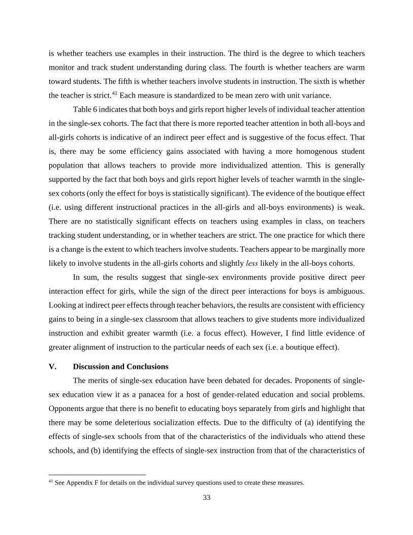
33

is whether teachers use examples in their instruction. The third is the degree to which teachers

monitor and track student understanding during class. The fourth is whether teachers are warm

toward students. The fifth is whether teachers involve students in instruction. The sixth is whether

the teacher is strict.41 Each measure is standardized to be mean zero with unit variance.

Table 6 indicates that both boys and girls report higher levels of individual teacher attention

in the single-sex cohorts. The fact that there is more reported teacher attention in both all-boys and

all-girls cohorts is indicative of an indirect peer effect and is suggestive of the focus effect. That

is, there may be some efficiency gains associated with having a more homogenous student

population that allows teachers to provide more individualized attention. This is generally

supported by the fact that both boys and girls report higher levels of teacher warmth in the single-

sex cohorts (only the effect for boys is statistically significant). The evidence of the boutique effect

(i.e. using different instructional practices in the all-girls and all-boys environments) is weak.

There are no statistically significant effects on teachers using examples in class, on teachers

tracking student understanding, or in whether teachers are strict. The one practice for which there

is a change is the extent to which teachers involve students. Teachers appear to be marginally more

likely to involve students in the all-girls cohorts and slightly less likely in the all-boys cohorts.

In sum, the results suggest that single-sex environments provide positive direct peer

interaction effect for girls, while the sign of the direct peer interactions for boys is ambiguous.

Looking at indirect peer effects through teacher behaviors, the results are consistent with efficiency

gains to being in a single-sex classroom that allows teachers to give students more individualized

instruction and exhibit greater warmth (i.e. a focus effect). However, I find little evidence of

greater alignment of instruction to the particular needs of each sex (i.e. a boutique effect).

V. Discussion and Conclusions

The merits of single-sex education have been debated for decades. Proponents of single-

sex education view it as a panacea for a host of gender-related education and social problems.

Opponents argue that there is no benefit to educating boys separately from girls and highlight that

there may be some deleterious socialization effects. Due to the difficulty of (a) identifying the

effects of single-sex schools from that of the characteristics of the individuals who attend these

schools, and (b) identifying the effects of single-sex instruction from that of the characteristics of

41 See Appendix F for details on the individual survey questions used to create these measures.

34

those schools that tend to be single-sex, the existing research literature has not been able to provide

conclusive evidence on the matter. This paper presents a context and empirical approach that

credibly addresses both empirical challenges. By exploiting exogenous variation in school

assignments, I isolate the effect of schools from that of students. By exploiting changes in single-

sex status within schools over time, I isolate the effect of single-sex instruction from that of the

characteristics of the schools that happen to provide single-sex instruction. I find that both sources

of bias are important, and that a failure to account for them both may lead to inaccurate estimates.

The results show that single-sex education can improve both boys’ and girls’ outcomes.

Three years after being assigned to a single-sex secondary school, both boys and girls have higher

scores on standardized tests. Five years later, they are more likely to take and pass advanced

courses. In the long run, both boys and girls are more likely to have completed secondary school

and to have earned the credential required to continue to tertiary education. Importantly, boys are

also less likely to have been arrested, and girls are less likely to be teen mothers. One limitation of

existing studies on single-sex education is the lack of evidence on mechanisms. This paper presents

some new results and analysis in this regard. First, the theoretical framework highlights that the

effect of single-sex education will depend on the nature of direct gender peer effects and also

indirect peer effects that operate through the behaviors of teachers in both single-sex and coed

environments. This is supported by survey results indicating that both direct and indirect peer

effect mechanisms may have played an important role.

Note that these benefits to single-sex instruction were achieved at zero additional financial

cost. The test score effect of roughly 0.2sd is about as large as the effect of going from a teacher

at the 5th percentile to one at the 50th percentile of effectiveness. To achieve comparable results

through increases in school spending, reductions in class size, tutoring, or other interventions

would require a nontrivial financial outlay. The results of this study illustrate the potential cost-

effectiveness of leveraging peer effects (both direct and indirect) to improve student outcomes

(both educational and otherwise). The evidence demonstrates that, in some contexts, single-sex

education can be an effective, low-cost way to improve outcomes for low-achieving students.

Further work is needed to better identify the contexts in which single-sex instruction is likely to

improve the outcomes of both girls and boys. The theoretical framework and the evidence on

mechanisms presented herein may guide future research in these areas.

35

Works Cited

Booth, Alison L., Lina Cardona-Sosa, and Patrick Nolen. 2013. "Do Single-Sex Classes Affect Exam Scores? An Experiment in a Coed University." IZA Discussion Paper Number 7207.

Black, Sandra E. & Paul J. Devereux & Kjell G. Salvanes, 2013. "Under Pressure? The Effect of Peers on Outcomes of Young Adults," Journal of Labor Economics, University of Chicago Press, vol. 31(1), pages 119 - 153.

Brame, Robert; Shawn Bushway, Raymond Paternoster and Michael Turner (2014) “Demographic Patterns of Cumulative Arrest Prevalence by Ages 18 and 23.” Crime and Delinquency 60:3:471-486.

Chade, H., Smith, L., 2006. Simultaneous search. Econometrica 74 (5), 1293–1307. Chavous, Kevin P. 2013. "Single-Sex Education: A Viable Option for Today's Students." The Huffington Post.

5 4. Accessed 3 5, 2015. http://www.huffingtonpost.com/kevin-p-chavous/singlesex-education-a-via_b_3015145.html.

Deming, David J., Justine S. Hastings, Thomas J. Kane, Douglas O. Staiger “School Choice, School Quality and Postsecondary Attainment”. 2014. American Economic Review, 104(3): 991-1014.

Deming DJ. Better Schools, Less Crime?. Quarterly Journal of Economics. 2011;126 (4) :2063-2115. Dee, Thomas S., Brian A. Jacob, Jonah E. Rockoff, and Justin, McCrary. 2011. "Rules and Discretion in the

Evaluation of Students and Schools: The Case of the New York Regents Examinations." Columbia University Mimeo.

Ding, Weili, Lehrer, Steven F., 2007. Do peers affect student achievement in China's secondary schools? The Review of Economics and Statistics 89 (2), 300–312.

Duflo, Esther, Pascaline Dupas, and Michael Kremer. 2011. "Peer Effects, Teacher Incentives, and the Impact of Tracking: Evidence from a Randomized Evaluation in Kenya." American Economic Review (101) 5: 1739-74.

Eliot, Lise “FORGET WHAT YOU THINK YOU KNOW ABOUT THE BENEFITS OF SINGLE-SEX SCHOOLING” Newsweek, December, 31, 2016.

Entwisle, Doris R., Karl L. Alexander, and Lina S. Olson. 2007. "Early Schooling: The Handicap of Being Poor and Male." Sociology of Education 114-138.

Fryer, Roland G. 2014. "Injecting Successful Charter School Strategies into Traditional Public Schools: Evidence From Field Experiments." Quarterly Journal of Economics 129 (3): 1355-1407.

Fryer, Roland G., and Steven D. Levitt. 2010. "An Empirical Analysis of the Gender Gap in Mathematics." American Economic Journal: Applied Economics (American Economic Association) 2 (2): 210-40.

Gale, David, and Shapley, Lloyd, 1962. College admissions and the stability of marriage. Am. Math. Mon. 69 (1), 9–15.

Hardwick Day 2008 “What Matters in College After College: A Comparative Alumnae Research Study” Heckman, James J., and Tim Kautz. 2012. "Hard evidence on soft skills." Labour Economics 19 (4): 451-464. Heckman, James. 1999. "Policies to Foster Human Capital." NBER Working Paper No 7288. Hoxby, Caroline M. 2000. "Peer effects in the classroom: Learning from gender and race variation." NBER

Working Paper no. 7867. Hoxby, Caroline and Gretchen Weingarth. 2006. “Taking Race Out of the Equation: School Reassignment and

the Structure of Peer Effects.” Presented at the 2006 American Economic Association Annual Meetings.

Howell, William, Martin West and Paul Peterson, “The 2008 Education Next–PEPG Survey” Education Next Fall 2008, pp. 12-26.

Jackson, C. Kirabo. (2010) "Do Students Benefit From Attending Better Schools?: Evidence From Rule-based Student Assignments in Trinidad and Tobago" The Economic Journal, 120(549): 1399-1429.

Jackson, C. Kirabo. 2013. "Can Higher-Achieving Peers Explain the Benefits to Attending Selective Schools?: Evidence from Trinidad and Tobago." Journal of Public Economics.

Jackson, C. Kirabo. 2013. "Non-Cognitive Ability, Test Scores, and Teacher Quality: Evidence from 9th Grade Teachers in North Carolina." NBER Workign Paper No 18624.

36

Jackson, C. Kirabo. 2012. "Single-sex schools, student achievement, and course selection: Evidence from rule-based student assignments in Trinidad and Tobago." Journal of Public Economics 96 (2012): 173-187.

Jacobs, Jerry A. 1996. "Gender Inequality and Higher Education." Annual Review of Sociology 22: 153-185. Kearney, Melissa S. and Phillip B. Levine. 2012. "Why Is the Teen Birth Rate in the United States So High and

Why Does It Matter?" Journal of Economic Perspectives, 26(2): 141-63. Ku, Hyejin, and Do Won Kwak. 2013. "Together or Separate: Disentangling the Effects of Single-Sex

Schooling from the Effects of Single-Sex Schools." University of Queensland Mimeo. Lavy, Victor, and Analia Schlosser. 2012. "Mechanisms and Impacts of Gender Peer Effects at School."

American Economic Journal: Applied Economics 3 (2): 1-33. Lee, Soohyung, Lesley J. Turner, Seokjin Woo, and Kyunghee Lim. 2014. "All or Nothing? The Impact of

School and Classroom Gender Composition on Effort and Academic Achievement." NBER Working Paper No 20722.

Lu, Fangwen, and Michael L. Anderson. 2015. “Peer Effects in Microenvironments: The Benefits of Homogeneous Classroom Groups”. Journal of Labor Economics 33 (1): 91–122.

McCrary, Justin, (2008), Manipulation of the running variable in the regression discontinuity design: A density test, Journal of Econometrics, 142, issue 2, p. 698-714.

Mael F., A. Alonso, D. Gibson, K. Rogers, and M. Smith. 2005. Single-sex Versus Coeducational Schooling: A Systematic Review. Washington, DC: US Department of Education.

Mann, Allison, and Thomas DiPrete. 2013. "Trends in Gender Segregation in the Choice of Science and Engineering Majors." Social Science Research 42: 1519-1541.

Oosterbeek, Hessel., Reyn van Ewijk "Gender peer effects in university: Evidence from a randomized experiment" Economics of Education Review Volume 38, February 2014, Pages 51–63

Park, Hyunjoon, Jere R. Behrman, and Jaesung Choi. 2013. "Causal Effects of Single-Sex Schools on College Entrance Exams and College Attendance: Random Assignment in Seoul High Schools." Demography 50 (2): 447-469.

Pop-Eleches, Cristian and Miguel Urquiola. 2013. "Going to a Better School: Effects and Behavioral Responses."American Economic Review, 103(4):1289-1324.

Ready, D. D., L. F. LoGerfo, D. T. Burkam, and V. E. Lee. 2005. "Explaining girls’ advantage in kindergarten literacy learning: Do classroom behaviors make a difference?" Elementary School Journal 21-38.

Rich, Motoko “Old Tactic gets New Use: Public Schools Separate Girls and Boys” New York Times Nov 30th 2014.

Rosenthal, Marjorie S., Joseph S. Ross, RoseAnne Bilodeau, Rosemary S. Richter, Jane E. Palley, and Elizabeth H. Bradley, “Economic Evaluation of a Comprehensive Teenage Pregnancy Prevention Program: Pilot Program” American Journal of Preventative Medicine. 2009 Dec; 37(6 Suppl 1): S280–S287.

Sharma, Amitabh. 2006. "University of the West Indies (UWI) moves to address gender imbalance - Institution initiates mentoring programmes." Jamaica Gleaner, December 18.

Steffensmeier, Darrell, and Emilie Allan. 1996. "GENDER AND CRIME: Toward a Gendered Theory of Female Offending." Annual Review of Sociology 459-87.

Stevens, W. David, Lauren Sartain, Elaine M. Allensworth, and Rachel Levenstein; with Shannon Guiltinan, Nick Mader, Michelle Hanh Huynh, and Shanette Porter. “Discipline Practices in Chicago Schools: Trends in the Use of Suspensions and Arrests” University of Chicago Report 2015.

Strain, Michael (2013) “Single-sex classes & student outcomes: Evidence from North Carolina” Economics of Education Review Volume 36, October 2013, Pages 73–87

The White House. 2012. Race to the Top High School Commencement Challenge. Accessed 3 3, 2015. http://www.whitehouse.gov/issues/education/k-12/commencement-challenge.

The World Bank. 2014. Ratio of female to male tertiary enrollment. Accessed 3 3, 2015. http://data.worldbank.org/indicator/SE.ENR.TERT.FM.ZS.

U.S. Department of Education. 2014. Digest of Education Statistics. National Center for Educational Statistics. Whitmore, Diane, “Resource and Peer Impacts on Girls' Academic Achievement: Evidence from a Randomized

Experiment," American Economic Review: Papers and Proceedings, 2005, 95 (2), 199-203.

37

Table 1: Summary Statistics

1 2 3 4 5 6

All Boys Taking

the SEA

Boys at All-Boy’s Pilot

Schools Pre-Transition

Boys at All-Boy’s Pilot

Schools Post-

Transition

All Girls

Taking the

SEA

Girls at All-Girl’s Pilot

Schools Pre-Transition

Girls at All-Girl’s Pilot

Schools Post-Transition

Assigned to Pilot School 0.184 0.906 0.925 0.175 0.921 0.946 (0.388) (0.292) (0.263) (0.380) (0.270) (0.227)

Times Repeated SEA 0.050 0.055 0.068 0.047 0.045 0.046 (0.218) (0.228) (0.251) (0.212) (0.208) (0.210)

Std. Total SEA Score -0.175 -0.588 -0.642 0.177 -0.368 -0.266 (1.055) (0.824) (0.798) (0.923) (0.721) (0.757)

Std. Math NCSE Score -0.175 -0.572 -0.702 0.183 -0.243 -0.117 (0.987) (0.819) (0.848) (0.960) (0.864) (0.784)

Std. English NCSE Score -0.251 -0.713 -0.721 0.254 -0.169 -0.101 (0.985) (0.836) (0.940) (0.933) (0.933) (0.796)

Std. Spanish NCSE Score -0.258 -0.700 -0.676 0.251 -0.168 -0.113 (0.964) (0.746) (0.873) (0.958) (0.900) (0.827)

Std. Science NCSE Score -0.173 -0.593 -0.700 0.171 -0.306 -0.194 (0.990) (0.786) (0.876) (0.961) (0.818) (0.744)

Std. Social Studies NCSE Score -0.188 -0.451 -0.590 0.273 -0.141 -0.008 (0.960) (0.875) (0.933) (0.946) (0.920) (0.844)

Std. Arts NCSE Score -0.187 -0.386 -0.522 0.190 0.016 -0.097 (0.962) (0.863) (0.960) (0.996) (0.961) (0.854)

Std. Physical Ed. NCSE Score -0.053 -0.301 -0.455 0.064 -0.220 -0.029 (1.015) (0.978) (1.068) (0.971) (0.946) (0.838)

Std. Technical NCSE Score -0.183 -0.174 -0.331 0.184 0.172 0.159 (0.933) (0.914) (0.928) (1.030) (1.037) (0.876)

Take the NCSE 0.835 0.849 0.847 0.872 0.870 0.852 (0.372) (0.358) (0.360) (0.335) (0.336) (0.355)

Take the CSEC 0.771 0.750 0.729 0.844 0.814 0.794 (0.420) (0.433) (0.444) (0.363) (0.389) (0.404)

Earn Secondary Certificate 0.317 0.120 0.106 0.458 0.239 0.214 (0.465) (0.325) (0.308) (0.498) (0.426) (0.410)

Arrested by age 16 0.034 0.045 0.032 0.007 0.010 0.007 (0.182) (0.208) (0.176) (0.081) (0.100) (0.082)

Arrested by age 18 0.075 0.105 0.059 0.014 0.020 0.011 (0.263) (0.307) (0.235) (0.116) (0.138) (0.106)

Baby by age 16 0.009 0.012 0.014 (0.093) (0.107) (0.117)

Baby by age 18 0.043 0.072 0.046 (0.203) (0.258) (0.209)

Observations 62953 6739 4627 61429 6051 4016 Notes: This dataset is based on the population of SEA takers during years 2006 through 2012. All SEA and NCSE scores are standardized to be mean zero and unit variance in each cohort. Earning a certificate means passing five subjects in the CSEC exams (10th grade) including math and English. This is the prerequisite to entering tertiary education. Summary statistics are provided for all boys and girls taking the SEA and also the subsample of boys and girls who attended the pilot school pre and post transition to single-sex. Standard errors are presented in parentheses.

38

Table 2: Effects of the All-Boys and All-Girls Transition in 6th Grade on Math Scores in 8th Grade

Math Score Predicted Math Score b. All Years Post Only a. All Years OLS OLS OLS 2SLS 2SLS 2SLS Boys Only (150,296 observations) 1 2 3 4 5 6

Boys-Pilot*POST -0.146** 0.0458 0.0905+ 0.334* -0.0958 0.000264 [0.0503] [0.0447] [0.0541] [0.168] [0.150] [0.0159] Girls Only (156,149 observations) 7 8 9 10 11 12

Girls-Pilot*POST 0.143** 0.0921* 0.161** 0.147+ 0.178+ 0.000258 [0.0361] [0.0370] [0.0509] [0.083] [0.0919] [0.0225] Both Boys and Girls (306,445 observations) 13 14 15 16 17 18

Pilot*POST 0.000865 0.0774* 0.120** 0.227* 0.0257 0.00615 [0.0731] [0.0314] [0.0388] [0.105] [0.107] [0.0110]

Test Scores N Y Y Y Y N Choices N N Y Y Y N Applicant Group N N N Y Y Y Robust standard errors in brackets adjusted for clustering at the assigned school level. ** p<0.01, * p<0.05, + p<0.1 Notes: Each column represents a separate regression. All models include the effect of attending a pilot school so that the coefficients on Boys-Pilot*POST and Girl-Pilot*POST represent the post-transition change in the effect of attending an all-boys pilot school and all-girls pilot school. The coefficient on Pilot*POST represents the difference between the effect of attending any pilot school after transition and attending any pilot school prior to transition. a. The post only models exclude the SEA cohorts prior to 2010. Accordingly, the number of observations for this model is less than that for

the full model. There are 62,011, 64,310, and 126,321 male, female, and total observations in the post only models, respectively. b. Predicted scores are fitted values from a regression of math scores on the number of SEA attempts (repeater status in 5th grade), the

student’s religion, indicators for the primary school, selectivity of the student’s first second third and fourth secondary school choices, month of birth (to measure quarter of birth effects), and age at SEA. Results using the predicted average of all academic subjects are similar.

39

Table 3: Nonlinear Effect on Test Scores on Eighth Grade Test Scores

Math

Missing Bottom 20% 21st to 40th Percentile

41st to 60th Percentile

61st to 80th Percentile Top 20%

Boys-Pilot*POST 0.046 -0.163* 0.0372 0.0322 -0.0101 0.0546* [0.0528] [0.0752] [0.0561] [0.0719] [0.0360] [0.0229] Girls-Pilot*POST -0.00114 -0.0341 0.0299 -0.105* 0.00446 0.105** [0.0371] [0.0551] [0.0608] [0.0516] [0.0365] [0.0319]

Academic Subjects

Missing Bottom 20% 21st to 40th Percentile

41st to 60th Percentile

61st to 80th Percentile Top 20%

Boys-Pilot*POST 0.0447 -0.0853 0.00789 -0.0992+ 0.0438+ 0.0582** [0.0517] [0.0791] [0.0422] [0.0517] [0.0263] [0.0197] Girls-Pilot*POST -0.000964 0.0385 0.0547 -0.132** -0.0218 0.0616** [0.0371] [0.0585] [0.0580] [0.0410] [0.0732] [0.0223]

All Subjects (Both Academic and Non-Academic Subjects)

Missing Bottom 20% 21st to 40th Percentile

41st to 60th Percentile

61st to 80th Percentile Top 20%

Boys-Pilot*POST 0.0447 -0.107 0.0115 -0.0641 0.00445 0.0807** [0.0517] [0.0667] [0.0560] [0.0433] [0.0285] [0.0217] Girls-Pilot*POST -0.000964 0.016 0.0582 -0.0582 -0.0279 0.0128 [0.0371] [0.0529] [0.0467] [0.0480] [0.0345] [0.0212] Robust standard errors in brackets adjusted for clustering at the assigned school level. ** p<0.01, * p<0.05, + p<0.1 Each column represents a separate regression. All models include the effect of attending a pilot school so that the coefficients on Boys-Pilot*POST and Girls-Pilot*POST represent the post-transition change in the effect of attending an all-boys pilot school and all-girls pilot school. All models include fourth order polynomial of incoming SEA test scores, cohort fixed effects, indicators for gender, cutoff fixed effects, and choice group indicator variables. The number of observations is larger than in the test score regressions because these models include observations that are missing NCSE test score data. The quintile dummies connote both taking the NCE exam and scoring at a particular quintile of the distribution. The male sample includes 180,932 observations and the female sample has 178,859 observations.

40

Table 4: Effects on Scores by Subject

Math English Spanish Science Social Studies Arts Technical

Physical Education

Boys and Girls Combined: 300,412 observations 1 2 3 4 5 6 7 8

Pilot*POST 0.227* 0.0546 0.243* 0.219 0.312* 0.136 0.395** 0.12 [0.105] [0.114] [0.118] [0.142] [0.150] [0.197] [0.135] [0.181]

Boys Only: 147,468 observations 9 10 11 12 13 14 15 16

Boys-Pilot*POST 0.334* 0.128 0.442** 0.319 0.534** 0.896* 0.416* 0.255 [0.168] [0.200] [0.166] [0.232] [0.200] [0.403] [0.191] [0.317]

Girls Only: 153,244 observations 17 18 19 20 21 22 23 24

Girls-Pilot*POST 0.147+ -0.069 0.0717 0.0825 -0.0435 -0.333* 0.238 -0.255 [0.083] [0.131] [0.165] [0.154] [0.118] [0.165] [0.212] [0.165]

Choice fixed effects Y Y Y Y Y Y Y Y App Group Fixed Effects Y Y Y Y Y Y Y Y SEA Scores Y Y Y Y Y Y Y Y Robust standard errors in brackets are adjusted for clustering at the assigned school level. ** p<0.01, * p<0.05, + p<0.1 Notes: Each column in each panel (top and bottom) represents a separate regression and is indicated with a specification number (1 through 20). The dependent variable is indicated in the top row. All models include the effect of attending a pilot school so that the coefficients on Boys-Pilot*POST and Girls-Pilot*POST represent the post-transition change in the effect of attending an all-boys pilot school and all-girls pilot school. Similarly, the coefficient on Pilot*POST represents the difference between the effect of attending any pilot school after transition and attending any pilot school prior to transition. All models include fourth order polynomial of incoming SEA test scores, cohort fixed effects, indicators for gender, cutoff fixed effects, and choice group indicator variables.

41

Table 5: Effects on Educational Attainment Outcomes (5 Years later)

Dropout Before 10th grade

Take Advanced

English

Take Advanced

Math

Take Full

Science Pass Math

Pass English

Subjects Taken

Subjects Passed

Earn Certificate

Boys and Girls Combined: 307,129 observations 1 2 3 4 5 6 7 8 9

Pilot*Post -0.0178 0.0796* 0.0495* 0.133** 0.115** 0.101** 0.211 0.485** 0.0744** [0.0557] [0.0310] [0.0223] [0.0370] [0.0198] [0.0344] [0.444] [0.170] [0.0186]

Boys Only: 154,616 observations 10 11 12 13 14 15 16 17 18

Boys-Pilot*Post -0.0155 0.100* 0.101** 0.110** 0.0842** 0.117** 0.523 0.677** 0.0533+ [0.0652] [0.0435] [0.0308] [0.0372] [0.0285] [0.0380] [0.536] [0.251] [0.0316]

Girls Only: 152,513 observations 19 20 21 22 23 24 25 26 27

Girls-Pilot*Post -0.0449 0.0703 0.0184 0.0884 0.171** 0.122* 0.319 0.530* 0.119** [0.0689] [0.0510] [0.0193] [0.0792] [0.0289] [0.0598] [0.549] [0.225] [0.0315]

Cutoff Fixed Effects Y Y Y Y Y Y Y Y Y Choice Fixed Effects Y Y Y Y Y Y Y Y Y SEA score Y Y Y Y Y Y Y Y Y Robust standard errors in brackets adjusted for clustering at the assigned school level. ** p<0.01, * p<0.05, + p<0.1 Notes: These outcomes are measured using the CSEC data from 2012-2016. As such, the regression results are only included for the SEA cohorts before 2012. Each column represents a separate regression. The dependent variable is indicated in the top row. All models include the effect of attending a pilot school so that the coefficients on Boys-Pilot*POST and Girls-Pilot*POST represent the post-transition change in the effect of attending an all-boys pilot school and all-girls pilot school. Similarly, the coefficient on Pilot*POST represents the difference between the effect of attending any pilot school after transition and attending any pilot school prior to transition. All models include fourth order polynomial of incoming SEA test scores, cohort fixed effects, indicators for gender, cutoff fixed effects, and choice group indicator variables.

42

Table 6: Effects on Arrests and Teen Births

Arrest by

16 Arrest by

17 Arrest by

18 Baby by 16 Baby by 17 Baby by 18 1 2 3 4 5 6 Boys Only: 154616 observations (excluding 2012)

Boys-Pilot * Post -0.0225 -0.0361+ -0.0601* - - - [0.0192] [0.0208] [0.0250] - - -

Girls Only: 178859 observations 7 8 9 10 11 12 Girls-Pilot * Post -0.00485 0.00291 0.00356 -0.0169 -0.0483* -0.0663*

[0.0115] [0.0124] [0.0147] [0.0143] [0.0222] [0.0334]

Choice Group Y Y Y Y Y Y Application Group Y Y Y Y Y Y SEA Scores Y Y Y Y Y Y Robust standard errors in brackets adjusted for clustering at the assigned school level. ** p<0.01, * p<0.05, + p<0.1 Each column represents a separate regression. The dependent variable is indicated in the top row. All models include the effect of attending a pilot school so that the coefficients on Boys-Pilot*POST and Girls-Pilot*POST represent the post-transition change in the effect of attending an all-boys pilot school and all-girls pilot school. All models include fourth order polynomial of incoming SEA test scores, cohort fixed effects, indicators for gender, cutoff fixed effects, and choice group indicator variables.

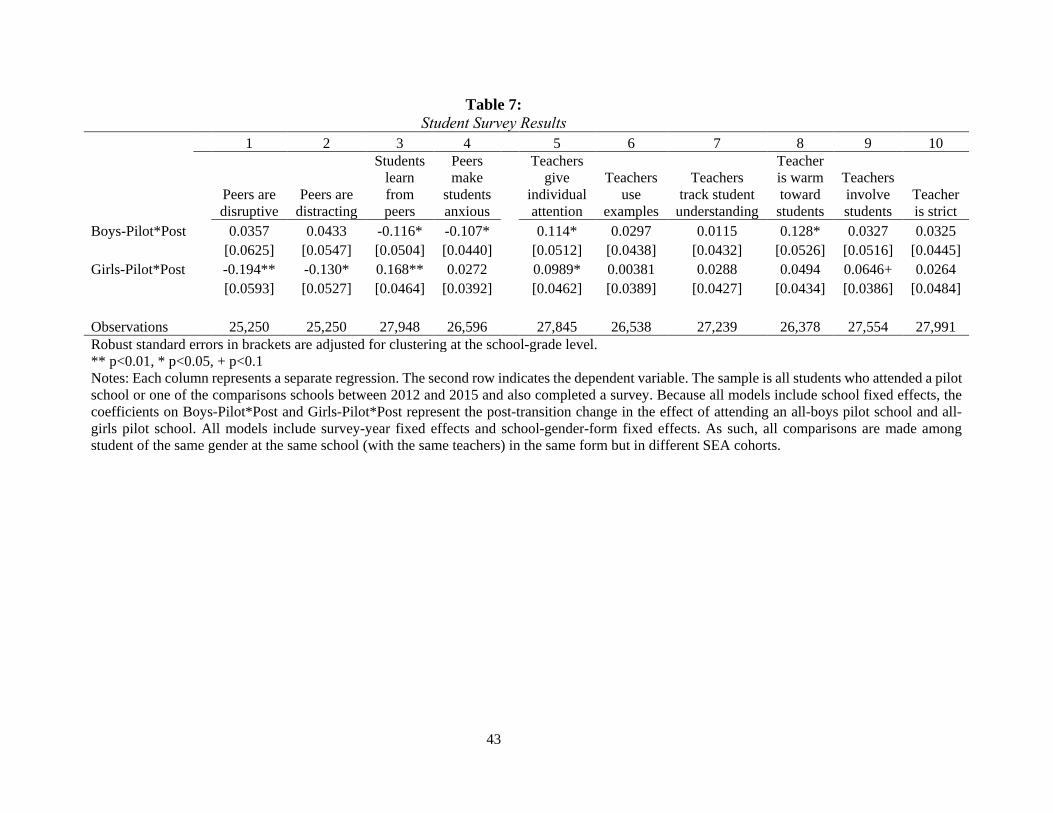
43

Table 7: Student Survey Results

1 2 3 4 5 6 7 8 9 10

Peers are disruptive

Peers are distracting

Students learn from peers

Peers make

students anxious

Teachers give

individual attention

Teachers use

examples

Teachers track student

understanding

Teacher is warm toward

students

Teachers involve students

Teacher is strict

Boys-Pilot*Post 0.0357 0.0433 -0.116* -0.107* 0.114* 0.0297 0.0115 0.128* 0.0327 0.0325 [0.0625] [0.0547] [0.0504] [0.0440] [0.0512] [0.0438] [0.0432] [0.0526] [0.0516] [0.0445]

Girls-Pilot*Post -0.194** -0.130* 0.168** 0.0272 0.0989* 0.00381 0.0288 0.0494 0.0646+ 0.0264 [0.0593] [0.0527] [0.0464] [0.0392] [0.0462] [0.0389] [0.0427] [0.0434] [0.0386] [0.0484]

Observations 25,250 25,250 27,948 26,596 27,845 26,538 27,239 26,378 27,554 27,991 Robust standard errors in brackets are adjusted for clustering at the school-grade level. ** p<0.01, * p<0.05, + p<0.1 Notes: Each column represents a separate regression. The second row indicates the dependent variable. The sample is all students who attended a pilot school or one of the comparisons schools between 2012 and 2015 and also completed a survey. Because all models include school fixed effects, the coefficients on Boys-Pilot*Post and Girls-Pilot*Post represent the post-transition change in the effect of attending an all-boys pilot school and all-girls pilot school. All models include survey-year fixed effects and school-gender-form fixed effects. As such, all comparisons are made among student of the same gender at the same school (with the same teachers) in the same form but in different SEA cohorts.

44

Figure 1: Predictors of Pilot School Status

This figure depicts the probability that each school was chosen as a pilot school as a function of the distance (as the crow flies) between that school and the nearest government school. Schools with below average selectivity have incoming SEA scores below the mean for all schools. Schools with above 75th percentile of selectivity have incoming SEA scores above the 75th percentile for all schools.

Government School with Below Average Selectivity

Non-Government School (Assisted or Private)

Government School Above 75th Percentile of Selectivity

0.1

.2.3

.4Pr

obab

ility

of B

eing

a P

ilot S

choo

l

0 1 2 3 4 5 6 7 8 9 10 11Distance to the Nearest Government School: Kilometers

Non-Selective Government Selective Government Non-Government

45

Figure 2: Example of cutoff based on school assignment for a single school in 2009 and 2010

This figure depicts the probability that a student applicant to pilot school X is assigned by the MOE to that school as a function of their incoming SEA score relative to the estimated cutoff for pilot school X. The probabilities are shown for raw SEA test scores. The dashed line is the estimated cutoff for school X. The top two panels present data for a school with high compliance with the cutoffs (in a pre and post transition year) and the lower two panels present data for a low compliance school (in a pre and post transition year).

46

Figure 3: Actual pilot attendance across pooled schools: pre and post transition

This figure depicts the probability that a student applicant to any pilot school attends a pilot school as a function of their incoming SEA score relative to the estimated cutoff for the pilot school to which they are an applicant. The standard deviation of SEA scores in 29. Following Pop-Eleches and Urquiola (2013), the data for the cutoffs for each pilot school in each year are stacked and the applicant's tests scores are centered around the respective cutoff. Relative scores below 0 are below the cutoff and those above 0 are above the cutoff. The dashed gray line is the location of the estimated aggregate cutoff. The figures show the estimated outcome for each test score bin. The 95 percent confidence interval for the outcome (from a linear regression of the outcome on a fourth order polynomial in test scores and a cutoff indicator) is presented.

47

Figure 4: Fuzzy RD in Math Scores across pooled schools in pre and post

This figure depicts the average math test score as a function of their incoming SEA score relative to the estimated cutoff for the pilot school to which they are an applicant. Following Pop-Eleches and Urquiola (2013), the data for the cutoffs for each pilot school in each year are stacked and the applicant's tests scores are centered around the respective cutoff. Relative scores below 0 are below the cutoff and those above 0 are above the cutoff. The dashed gray line is the location of the estimated aggregate cutoff. The standard deviation of the incoming test scores is 29. The top panel shows the estimated outcome for each relative test score. The 95 percent confidence interval for the outcome (from a linear regression of the outcome on a fourth order polynomial in test scores and a cutoff indicator) is presented. For a clearer presentation of the data around the cutoff, the lower panel presents the same data as the top panel but removing smooth functions of the running variable (fourth order polynomial).

-.3-.2

-.10

.1.2

-30 -20 -10 0 10 20 30SEA Score Relative to Pilot School Cut-Off

Pre-Transition

-.3-.2

-.10

.1.2

-30 -20 -10 0 10 20 30SEA Score Relative to Pilot School Cut-Off

Post-Transition

Residual Plot (removing fourth order polynomial of relative score)

-.2-.1

0.1

.2

-30 -20 -10 0 10 20 30SEA Score Relative to Pilot School Cut-Off

Pre-Transition

-.2-.1

0.1

.2

-30 -20 -10 0 10 20 30SEA Score Relative to Pilot School Cut-Off

Post-Transition

Residualized Math Scores Through Cut-Off

48

Figure 5: RD Estimates Over Time (Event Study)

Notes: Each data point represents the 2SLS regression estimate of attending a pilot school three years before and after the transition. The endogenous variables are attending a pilot school in 2007, 2008, 2009, 2010, 2011, and 2012. The excluded instruments are indicator variables denoting scoring above the threshold for an all-male or an all-female pilot school in 2007, 2008, 2009, 2010, 2011, and 2012. All models include fourth order polynomials of incoming test score, cohort fixed effects, gender fixed effects, and choice group fixed effects. Standard errors are adjusted for clustering at the assigned school level.

-.4-.2

0.2

.4

2007 2008 2009 2010 2011 2012Year

90% CI of Regression Prediction 90% CI of Data PointEffect on Standardized Math Scores

Effect of Attending a Pilot School on Math Scores: By Year

49

Figure 6: Accounting for Treatment Heterogeneity in the Pilot School Effect

Notes: Each data point represents the 2SLS regression estimate of the attending a pilot school after the transition relative to pre-transition. In each model, the pilot school indicator is interacted with a pre-treatment covariate to account for possible pilot-school treatment heterogeneity. The endogenous variables are attending a pilot school pre and post transition and the interaction between pre-treatment covariates and attending a pilot school. The excluded instruments are indicator variables denoting whether a student scored above the threshold for a pilot school, whether a student scored above the threshold for a pilot school in 2010 or after, and interactions between these instruments and pre-treatment student characteristics. All models include fourth order polynomials of incoming test score, cohort fixed effects, gender fixed effects, and choice group fixed effects. Model 0 is the baseline model. Each model 1-10 includes interactions with pilot boy and girl school attendance and observed student characteristics. Model 1 includes interactions between attending a pilot school and incoming SEA scores. Models 2 and 3 include interactions between attending a pilot school and whether the student's top choice school was single-sex, and the number of single-sex schools in the student’s choice set, respectively. Models 4 and 5 includes interactions between attending a pilot school and the average SEA of the top choice school and the average selectivity of schools in the student’s choice set, respectively. Model 6 includes interactions between attending a pilot school and the average SEA scores at the student’s primary school. Model 7 includes interactions between attending a pilot school and the fraction of own gender peers at the student’s primary school. Model 8 includes interactions between attending a pilot school and predicted math scores (predicted math scores are based on the number of SEA attempts (repeater status in 5th grade), the student’s religion, indicators for the primary school, selectivity of the student’s first second third and fourth secondary school choices, month of birth (to measure quarter of birth effects), and age at SEA). Model 9 includes interactions with the average selectivity of the students next ranked school (i.e. the counterfactual school), and Model 10 includes interactions with the percentile rank of the school ranked just below the pilot school.

50

FOR ONLINE PUBLICATION

Appendix A: Proofs for Claims in Theoretical Section

Student outcomes are given by (1) where Yijg is the outcome of student i with teacher j of

gender 𝑔𝑔 ∈ {𝑔𝑔𝑔𝑔𝑔𝑔𝑔𝑔, 𝑏𝑏𝑏𝑏𝑏𝑏}, Gi is an indicator equal to 1 if student i is a girl and 0 otherwise. �̅�𝐺𝑗𝑗is the share of girls in class with teacher j, the proportion of time that teacher j aligns instruction to girls is 𝑝𝑝𝑗𝑗 ∈ [0,1], and uij is a random mean zero error term. (A1) 𝑌𝑌𝑖𝑖𝑗𝑗𝑖𝑖 = 𝛼𝛼𝐺𝐺𝑖𝑖 + 𝑓𝑓𝑖𝑖��̅�𝐺𝑗𝑗� + ℎ𝑖𝑖𝑝𝑝𝑗𝑗 + 𝜓𝜓�2𝑝𝑝𝑗𝑗 − 1� + 𝑢𝑢𝑖𝑖𝑗𝑗. The term 𝑓𝑓𝑖𝑖��̅�𝐺𝑗𝑗� captures the direct gender peer effect that operates through peer interactions. To allow for differential responses to the proportion of female classmates by males and females, I include the subscript g on 𝑓𝑓𝑖𝑖. The term, ℎ𝑖𝑖𝑝𝑝𝑗𝑗 captures the idea that that certain teaching practices may benefit girls more than boys and vice versa. Where 𝑝𝑝𝑗𝑗 is the proportion of time the teacher spends “aligning” classroom practices to the needs of girls, ℎ𝑖𝑖𝑖𝑖𝑟𝑟𝑟𝑟𝑟𝑟 ≥ 0 and ℎ𝑏𝑏𝑏𝑏𝑏𝑏𝑟𝑟 ≤ 0. The term 𝜓𝜓�2𝑝𝑝𝑗𝑗 − 1� captures the idea that there may be some efficiency gains for teachers associated with focusing their instruction to one group (either boys or girls). A teacher’s payoff is an increasing function of the outcomes of her class 𝑊𝑊(𝑌𝑌𝑖𝑖∈𝑗𝑗) so that 𝜕𝜕𝑊𝑊/𝜕𝜕𝑌𝑌𝑖𝑖 > 0 ∀𝑔𝑔 ∈ 𝑗𝑗. Teachers chose how much time to spend aligning instruction to girls (𝑝𝑝𝑗𝑗) in order to maximize their individual payoff. Proposition 1: Teachers will employ entirely male-aligned instruction in all-male classrooms and entirely female-aligned instruction in all-female classrooms Proof: If the classroom is all-boys, then the for all 𝑔𝑔 ∈ 𝑗𝑗, ℎ𝑖𝑖𝑝𝑝𝑗𝑗 < 0, so that (𝑌𝑌𝑖𝑖𝑗𝑗�𝑝𝑝𝑗𝑗 = 0� >(𝑌𝑌𝑖𝑖𝑗𝑗�𝑝𝑝𝑗𝑗 ≠ 0�. By assumption, 𝜕𝜕𝑊𝑊/𝜕𝜕(𝑌𝑌𝑖𝑖) > 0 𝑓𝑓𝑏𝑏𝑔𝑔 𝑎𝑎𝑔𝑔𝑔𝑔 𝑔𝑔 ∈ 𝑗𝑗, so that 𝑊𝑊(𝑌𝑌𝑖𝑖∈𝑗𝑗�𝑝𝑝𝑗𝑗 = 0� >𝑊𝑊(𝑌𝑌𝑖𝑖∈𝑗𝑗|𝑝𝑝𝑗𝑗 ≠ 0). As such, teachers in all-boys classes will chose to align instruction to boys. Similarly, if the classroom is all-girls, then the for all 𝑔𝑔 ∈ 𝑗𝑗, ℎ𝑖𝑖𝑝𝑝𝑗𝑗 > 0, so that (𝑌𝑌𝑖𝑖𝑗𝑗�𝑝𝑝𝑗𝑗 = 0� <(𝑌𝑌𝑖𝑖𝑗𝑗�𝑝𝑝𝑗𝑗 ≠ 0�. By assumption, 𝜕𝜕𝑊𝑊/𝜕𝜕(𝑌𝑌𝑖𝑖) > 0 𝑓𝑓𝑏𝑏𝑔𝑔 𝑎𝑎𝑔𝑔𝑔𝑔 𝑔𝑔 ∈ 𝑗𝑗, so that 𝑊𝑊(𝑌𝑌𝑖𝑖∈𝑗𝑗�𝑝𝑝𝑗𝑗 = 0� <𝑊𝑊(𝑌𝑌𝑖𝑖∈𝑗𝑗|𝑝𝑝𝑗𝑗 ≠ 0). As such, teachers in all-girls classes will chose to align instruction to girls. Proposition 2: In mixed-gender classrooms, some teachers may align instruction to girls all the time, others may align instruction to boys all the time, and some teachers may align instruction to boys and girls some of the time. The choice of how to align instruction will depend on the specific parameters of the production function and the incentives faced by teachers and cannot be determined ex-ante. I outline three illustrative cases. In all cases, I make the assumption that teacher utility is a weighted average of the utility for each student in her class, so that 𝑊𝑊(𝑌𝑌𝑖𝑖∈𝑗𝑗) = ∑ 𝑔𝑔(𝑏𝑏𝑖𝑖)𝑖𝑖∈𝑗𝑗 . Case 1a: If the costs of adopting a mixed strategy are sufficiently large (i.e. ψ is very large), and teachers payoffs are convex in individual student test scores, then teachers will choose to align

51

instruction only to girls. Intuitively, with very large costs to adopting a mixed strategy, teachers will align instruction to only girls or only boys even in mixed-gender classrooms. If teacher payoffs are convex in individual student scores, then the marginal increase in utility will be higher for increasing tests scores at the top of the distribution than at the bottom. Because girls are more highly represented at the top of the distribution, teachers will choose only girl aligned instruction in coed classrooms. Case 1b: If the costs of adopting a mixed strategy are sufficiently large (i.e. ψ is very large), and teacher payoffs are concave in individual student test scores, then teachers will choose to align instruction only to boys. Intuitively, with very large costs to adopting a mixed strategy, teachers will align instruction to only girls or only boys even in mixed-gender classrooms. If teacher payoffs are concave in individual student scores, then the marginal increase in utility will be higher for increasing tests scores at the bottom of the distribution. Because boys are more highly represented at the bottom of the distribution, teachers will choose only boy aligned instruction in coed classrooms. Proof: Assume that the distribution of female incoming achievement has the same shape as that of males, but is a right shift of that for males by some positive constant a -- this is consistent with my data. If the teacher aligns instruction to males/females, then the male/female latent outcome distribution is shifted to the right by some constant δ (i.e. ℎ𝑖𝑖𝑝𝑝𝑗𝑗=−(ℎ𝑏𝑏𝑝𝑝𝑗𝑗) = 𝛿𝛿). For each percentile, p, of the male distribution with latent outcome 𝑏𝑏𝑝𝑝,𝑚𝑚𝑁𝑁𝑟𝑟𝑁𝑁

𝑟𝑟𝑁𝑁𝑠𝑠𝑁𝑁𝑠𝑠𝑠𝑠 , there is a female with latent outcome 𝑏𝑏𝑝𝑝,𝑚𝑚𝑁𝑁𝑟𝑟𝑁𝑁𝑟𝑟𝑁𝑁𝑠𝑠𝑁𝑁𝑠𝑠𝑠𝑠 + 𝑎𝑎. If the teacher aligns instruction to males, then the increase in payoff for the teacher is 𝑊𝑊�𝑏𝑏𝑝𝑝,𝑚𝑚𝑁𝑁𝑟𝑟𝑁𝑁

𝑟𝑟𝑁𝑁𝑠𝑠𝑁𝑁𝑠𝑠𝑠𝑠 + 𝛿𝛿, ∙� −𝑊𝑊(𝑏𝑏𝑝𝑝,𝑚𝑚𝑁𝑁𝑟𝑟𝑁𝑁𝑟𝑟𝑁𝑁𝑠𝑠𝑁𝑁𝑠𝑠𝑠𝑠 , ∙ ) for that student. If the teacher aligns instruction to females,

then the increase in payoff for the teacher is 𝑊𝑊�𝑏𝑏𝑝𝑝,𝑚𝑚𝑁𝑁𝑟𝑟𝑁𝑁𝑟𝑟𝑁𝑁𝑠𝑠𝑁𝑁𝑠𝑠𝑠𝑠 + 𝑎𝑎 + 𝛿𝛿, ∙� −𝑊𝑊(𝑏𝑏𝑝𝑝,𝑚𝑚𝑁𝑁𝑟𝑟𝑁𝑁

𝑟𝑟𝑁𝑁𝑠𝑠𝑁𝑁𝑠𝑠𝑠𝑠 + 𝑎𝑎, ∙ ) for the analogous female student. If teacher payoffs are convex, then 𝑊𝑊�𝑏𝑏𝑝𝑝,𝑚𝑚𝑁𝑁𝑟𝑟𝑁𝑁

𝑟𝑟𝑁𝑁𝑠𝑠𝑁𝑁𝑠𝑠𝑠𝑠 + 𝑎𝑎 + 𝛿𝛿, ∙� −𝑊𝑊�𝑏𝑏𝑝𝑝,𝑚𝑚𝑁𝑁𝑟𝑟𝑁𝑁

𝑟𝑟𝑁𝑁𝑠𝑠𝑁𝑁𝑠𝑠𝑠𝑠 + 𝑎𝑎, ∙ � > 𝑊𝑊�𝑏𝑏𝑝𝑝,𝑚𝑚𝑁𝑁𝑟𝑟𝑁𝑁𝑟𝑟𝑁𝑁𝑠𝑠𝑁𝑁𝑠𝑠𝑠𝑠 + 𝛿𝛿, ∙� −𝑊𝑊(𝑏𝑏𝑝𝑝,𝑚𝑚𝑁𝑁𝑟𝑟𝑁𝑁

𝑟𝑟𝑁𝑁𝑠𝑠𝑁𝑁𝑠𝑠𝑠𝑠 , ∙ ) for all percentiles of the male distribution so that the teacher’s payoff is higher if she aligns instruction to females. Conversely, if teacher payoffs are concave, then this inequality is reversed for all percentiles of the male distribution so that the teacher’s payoff is higher if she aligns instruction to males. Case 3: If ψ is small, teachers may adopt some mixed approach. In the extreme case where there is no cost to adopting a mixed strategy, teacher payoffs are linear in the average for the classroom, there are equal number of boys and girls in the classroom, and boys and girls are equally responsive to alignment, teachers will be indifferent between adopting a mixed strategy or aligning instruction to only one sex. In such cases, a mixed strategy may be adopted in coeducation classrooms. Proof: With linear payoffs, equal numbers of boys and girls, and equal responsiveness to alignment for boys and girls, the teachers expected payoff function under female alignment minus her payoff under male alignment is 𝜏𝜏[ℎ𝑖𝑖(𝑝𝑝) − ℎ𝑏𝑏(𝑝𝑝)], where 𝜏𝜏 is some scalar. If the average marginal effect of alignment is the same for both male and female students, then ℎ𝑖𝑖(𝑝𝑝) = ℎ𝑏𝑏(𝑝𝑝) ∀ 𝑝𝑝, so that 𝜏𝜏�ℎ𝑖𝑖(1) − ℎ𝑏𝑏(1)� = 0. In such a scenario, teachers are indifferent between aligning instruction to boys only, girls only, or adopting some mixed strategy. It is easy to come up with other scenarios in which teacher will chose some mixed strategy.

52

Appendix B: Single-sex Status by Year and Grade in Pilot Schools

Appendix Table B1: Status of Grades by Academic Year and Grade

Calendar Year Admitted Form 1 (6th grade) class 2009 2010 2011 2012 2013 2014 2015 Grade 6 Coed Single-Sex Single-Sex Single-Sex Single-Sex Coed Coed Grade 7 Coed Coed Single-Sex Single-Sex Single-Sex Single-Sex Coed Grade 8 Coed Coed Coed Single-Sex Single-Sex Single-Sex Single-Sex Grade 9 Coed Coed Coed Coed Single-Sex Single-Sex Single-Sex Grade 10 Coed Coed Coed Coed Coed Single-Sex Single-Sex

Note that the single-sex pilot program was started for the 2010 SEA cohort and was abandoned for the 2014 SEA cohort.

53

Appendix C: The School Assignment Algorithm

School slots are assigned in rounds such that the most highly subscribed/ranked school fills

its spots in the first round, then the next highly subscribed school fills its slots in the second round, and so on until all school slots are filled. This is done as follows: (1) the number of school slots at each school nj is predetermined based on capacity constraints. (2) Each student is tentatively placed in the applicant pool for her first choice school and is ranked by SEA score. (3) The school at which the njth ranked student has the highest SEA score is determined to be the most highly subscribed/ranked school and the top nj1 students in the applicant pool for top-ranked school j1 are admitted to school j1. The SEA score of the nj1-th student is the cutoff score for school j1. (4) The top-ranked school slots and the admitted students are removed from the process, and the second choice becomes the new "first choice" for students who had the top-ranked school as their first choice but did not gain admission. (5) This process is repeated in round two to assign students to the second highest ranked school j2 and determine the cutoff score for the second-ranked school, and this is repeated in subsequent rounds until all slots are filled. This assignment mechanism is a deferred acceptance algorithm (Gale and Shapley, 1962) in which students have incentives to truthfully reveal their rankings among chosen schools.

While the optimal set of school choices is difficult to solve, Chade, and Smith (2006) demonstrate that the choice set should include the school with the largest expected payoff (utility conditional on attendance times the likelihood of admission), students should rank selected schools in order of actual preferences, and should include a “reach” school for which admission is unlikely but the utility conditional on attendance is high.

This process is used to assign over 90% of all students. As such, as a practical matter, one can consider this applying to all students. However, there are a few exceptions to this rule. First, Government Assisted schools (not analyzed in this study) are allowed to admit 20% of their incoming class at the principal’s discretion. None of the pilot school is Government assisted so that there is no problem of principals hand picking students at the pilot schools. However, there are also assignments that do not follow this rule because students who do not score high enough to be assigned to a school on their choice list receive an administrative assignment from the Ministry of Education (these assignments are made to balance space considerations). Finally, due to unforeseen circumstances some schools may have less capacity than expected or may close (this may happen due to flooding etc.). In such rare cases, the Ministry will assign students to schools based on open slots in nearby schools, open slots in other schools in the choice list, and proximity.

I aim to use this assignment rule to isolate exogenous variation to the 20 pilot schools. A key feature of this assignment rule is that each school has a test score cutoff above which applicants are very likely to be assigned and below which applicants are very unlikely to be assigned. Even though the cutoffs are not known to the public and not all the administrative assignments follow the cutoff rule (due to a few exceptions made by the MOE), because I have access to the administrative assignment (which is outside the control of the students or their parents), the cutoffs can be recovered empirically for the 20 pilot schools.

54

Appendix D: Robustness Checks and Test of Validity

Validity of the RD Variation

The exogenous variation used in this paper is driven by the test-score cutoffs. Even though there is no way to prove for certain that the cutoff variation is valid, here I present evidence that this identification strategy is valid. One key diagnostic is to test for excess density above the cutoff and less than expected density below the cutoff (McCrary 2008). The first prima facie evidence of no change in density through the cutoff is simply the histogram of relative scores. As one can see in Figure 3, there is no uncharacteristic spike in density above the cutoff or dip in density just below the cutoff. If one computes the density of observations at each relative score and regresses this on scoring above the cutoff along with smooth functions of the relative score, there is no statistically significant relationship between scoring above the cutoff and the density. The point estimate is -0.0006 (p-value=0.53) – negative and not statistically significant. Taken together, the patterns suggest that the variation due to the test score cutoffs is likely valid. The other common test is for smoothness of latent outcomes (as proxied by covariates) through the cutoffs. In presenting the results I present effects on both actual outcomes and predicted outcomes (based on covariates) that show that the cutoff variation in pilot school attendance is not associated with any changes in predicted outcomes – consistent with the cutoff variation being valid.

Section III.D shows that there is little evidence of gaming around the cutoffs regarding the density of observation at each test score. However, the validity of the design also requires that there be no sorting of students around the cutoff (i.e. that latent outcomes are smooth through the cutoff). Given that students are unaware of the location of the cutoffs and are forced to make school choices before they take the SEA examinations, it is very unlikely that there is any sorting around the test score cutoffs. However, to provide further evidence that the variation employed (due to the cutoffs) is valid, I create a predicted math score variable and test for whether the 2SLS model (using the cutoff variation) predicts any change in predicted math scores.

Specifically, I regress the NCES math score on the number of SEA attempts (repeater status in 5th grade), the student’s religion, indicators for the primary school, selectivity of the student’s first second third and fourth secondary school choices, month of birth (to measure quarter of birth effects), and age at SEA. These variables are very strong predictors of math scores such that they yield an R-squared of 0.45. I then take the fitted value from this regression as my predicted math score. If there is some gaming of the cutoff, one would likely see that attending a pilot school as a result of scoring above the cutoff should be associated with better “predicted” scores. However, with no gaming there should be no relationship between scoring above the cutoff and one’s predicted score. Consistent with no gaming, there is no relationship between scoring above the cutoff and one’s predicted math score. Column 7 of Table 3 shows the estimated effect on predicted math scores for the all-boys pilot schools. The coefficients on the variables of interest are both small and statistically insignificant – indicating no gaming of the cutoff to the all-boys pilot schools. Column 7 of Table 4 shows the estimated effect on predicted math scores for the all-girls pilot schools. As with the boy’s schools, the coefficients on the variables of interest are both small and statistically insignificant – indicating no gaming of the cutoff to the all-girls pilot schools. Results for predicted average academic scores are very similar. As an additional check on this model, I estimated the effect on math scores and also on predicted math score (without controlling for choices) for different bandwidths around the cutoff. Appendix Figure D2, present these results visually. As one can see for any choice of bandwidth, there are large positive effects on math

55

scores and no effect on predicted math scores. Another concern one may have is that the 2SLS effects driven by the cutoffs could have happened by random chance by choosing any 20 random schools and any arbitrary cutoffs. To assuage this concern, I randomly chose 20 schools to be placebo pilot schools and for each school I assigned random “placebo” cutoffs to each placebo pilot school. I then estimated the effect on math scores of scoring above the cutoff for a pilot school after the transition (after 2010) relative to before. I did this with a new random draw of placebo pilot schools and cutoffs 2000 times and compared the placebo estimates to the actual estimate using the actual cutoffs. The real cutoff effect is 0.154 (p-value<0.01). Only 21 out of the 2000 placebo cutoffs was as large as the actual cutoff effect. Also, none of the z-scores for the estimated effects were as large as the actual z-score of 5.4. This indicates that the estimated cutoff effect (and the associated 2SLS estimates) is much larger than on might expect by random chance if there were indeed no single-sex effect. Validity of DiD Variation For the DiRD estimates to represent the causal effect of single-sex education requires that there were no changes in the pilot schools over time that coincided with the pilot program. Confounding changes within schools is unlikely because, (a) the individual schools had no control over when they would become pilot schools, (b) the government stipulated that no other changes take place in these schools, and (c) schools were not made aware of the changes until the summer preceding the change so that schools had no time to react before the start of the school year. Even so, one may worry that the pilot schools were already on an upward trajectory prior to transition. To show evidence that this does not drive the results, Figure 5 presents the RD estimates for attending a pilot school for each year three years before and three years after the transition on math scores. Each data point is an RD point estimate, and the 90 percent confidence interval is presented for each RD estimate. The figure also presents 90 percent confidence interval of the regression fit where the mean outcomes for the pre and post transition are pooled across individual years (as in the actual regression models). The RD estimates for 2007 through 2009 hover around -0.13, and there is no indication of an upward trend at pilot schools prior to the transition. Consistent with the positive single-sex effects for boys and girls, the pilot school effects in 2010, 2011 and 2012 are higher than that in the pre-treatment years and hover around 0.08. The difference between the RD estimates pre and post transition suggest that the transition increased the RD pilot school effect by roughly 0.13+0.08=0.21sd —in line with Table 2. Importantly, Figure 5 presents a clear visual representation of the DiD variation employed and provides compelling evidence that the DiD identifying common trends assumption is valid.

Even though the MOE clearly stipulated that there be no changes, as a final check on the DiD assumptions of no other changes, I used survey data collected by the MOE on a sample of teachers at all schools obtained in 2009 and 2013 to see if there were any systematic personnel changes that occured during the transition. In a simple difference in difference regression model predicting school level teacher characteristics with school fixed effects and year fixed effects (Appendix Table D1), between 2009 and 2013 the transition schools saw no differential change in the percentage of female teachers, or the percentage of teachers with a Bachelor’s degree. There is a marginally statistically significant effect on year-of-birth at the all-male pilot schools. This is consistent with sampling variability and is in the opposite direction of what would be required to generate a positive transition effect for the all-male pilot schools. I also explore if differences in class size (proxied by cohort size) can explain the results. In a simple model predicting initial cohort size (i.e. the size of the assigned cohort) with school fixed effects and year fixed effects,

56

the post-transition pilots have no statistically significant differences in cohort size (and the effect for the all-male and all-female pilot schools are in opposite directions). The results corroborate the notion that there were no other changes at pilot schools.

Appendix Figure D1: Distribution of Incoming SEA Scores around the cutoff

For each relative SEA score for each cutoff, the density of observations is computed. This figure represents the density of incoming SEA test scores relative to the test score of the applicant student. The cutoff for the school to which the student has applied is 0.

0.0

05.0

1.0

15D

ensi

ty

-150 -100 -50 0 50 100SEA Score Relative to Cut-Off (Pilot Schools Only)

57

Appendix Figure D2: RD Effect on Actual Math Scores and Predicted Math Scores by Bandwidth

This graph depicts the estimated 2SLS regression estimated transition effect on predicted math scores (Left) and actual math scores (Right) in a model with cutoff fixed effects, cohort fixed effect and a fourth order polynomial in test scores only (i.e. no additional controls for demographic or choices). The estimates for boys are on the top panel and those for girls in the lower panel. The 2SLS models are estimated among observations within a particular bandwidth of the cutoffs. The estimated 2SLS single-sex transition effects are reported for each bandwidth between 15 (0.5sd) and 90 (3sd). The 90 percent confidence interval for the estimate is presented in light grey, and the 95% confidence interval is in dark gray.

-.20

.2.4

.6

15 30 45 60 75 90Bandwidth

RD Effect on Predicted Math Scores: Girls

-.20

.2.4

.6

15 30 45 60 75 90Bandwidth

RD Effect on Math Scores: Girls

-.20

.2.4

.6

15 30 45 60 75 90Bandwidth

RD Effect on Predicted Math Scores: Boys

-.20

.2.4

.6

15 30 45 60 75 90Bandwidth

RD Effect on Math Scores: Boys

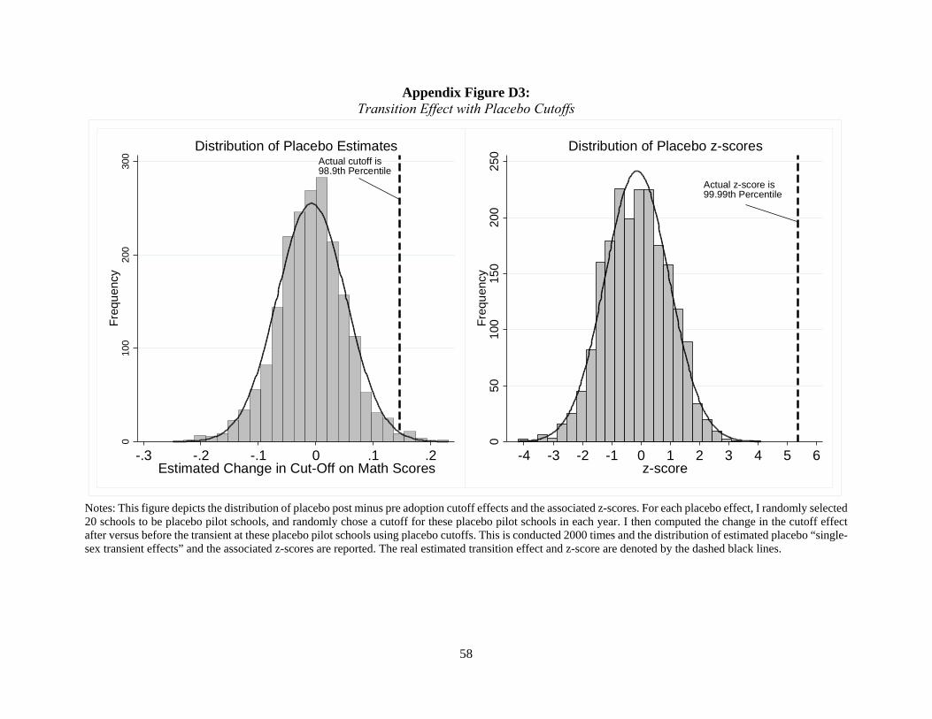
58

Appendix Figure D3: Transition Effect with Placebo Cutoffs

Notes: This figure depicts the distribution of placebo post minus pre adoption cutoff effects and the associated z-scores. For each placebo effect, I randomly selected 20 schools to be placebo pilot schools, and randomly chose a cutoff for these placebo pilot schools in each year. I then computed the change in the cutoff effect after versus before the transient at these placebo pilot schools using placebo cutoffs. This is conducted 2000 times and the distribution of estimated placebo “single-sex transient effects” and the associated z-scores are reported. The real estimated transition effect and z-score are denoted by the dashed black lines.

Actual z-score is99.99th Percentile

050

100

150

200

250

Freq

uenc

y

-4 -3 -2 -1 0 1 2 3 4 5 6z-score

Distribution of Placebo z-scoresActual cutoff is98.9th Percentile

010

020

030

0Fr

eque

ncy

-.3 -.2 -.1 0 .1 .2Estimated Change in Cut-Off on Math Scores

Distribution of Placebo Estimates

59

Appendix Table D1: Evidence of no other Changes

1 2 3 4 Teacher Variables at School-Year Level Female BA Degree Year of Birth Cohort Size

Girls-Pilot*Post 0.0243 0.108 -0.469 5.534 [0.0473] [0.131] [1.325] [10.75]

Boys-Pilot*Post 0.0287 -0.0254 1.413+ -12.36 [0.0279] [0.177] [0.788] [14.53]

Years 2008 & 2013 2006-2012 Observations 240 240 240 1,060 Robust standard errors in brackets ** p<0.01, * p<0.05, + p<0.1 These models are simple difference-in-difference regression models that include school fixed effects, year fixed effects, and an indicator for being a pilot school post-transition Girls-Pilot*Post and Boys-Pilot*Post. Models 1,2 and 3 are based on a survey on teachers administered in 2008 and 2013. Column 4 is based on the administrative SEA data for years 2006 through 2012. Cohort Size is the admitted cohorts size.

60

Appendix E: Evidence of Changes in Applicant Pool

After the transition from coed to single-sex, the applicant pool to the pilot schools changed.

To gain a sense of this, I regressed listing a pilot school as a first choice, second choice, third choice, and fourth choice on a simple Post indicator denoting whether the observation is for an SEA cohort in 2010 or after. The constant term and the coefficient on Post are reported in Table E1. The constant term represents the proportion of the sample that lists a pilot school in their choices during the pre-transition period, and the coefficient on Post is the change in proportion after the transition. The constant terms in Models 1 through 4 show that the pilot boy schools were typically listed as students third of fourth choices. About 8.5 percent have it as a third choice and 8.5 percent list an all-boys pilot as the fourth choice, while the comparable numbers for the first and second choice are about 2.7 and 5.5 percent, respectively. After the transition, boys were 0.4 percentage points more likely to list an all-boys pilot as their second choice, 2.54 percentage points more likely to list an all-boys pilot as their third choice, and to 6.36 percentage points more likely to list an all-boys pilot as their fourth choice. Some of this increased demand would have come from boys who would have listed the all-girls pilot switching over to the all-boys pilot, so that this may not be indicative of increased demand for all-boys schooling. To assess this, the dependent variable in models 5 through 8 is listing any pilot school as a first, second third or fourth choice. If students were indifferent to the change and simply listed the all-boys school in each pair if they would have chosen the all-girls pilot school, there should be no effect on choosing any pilot school. The coefficient on the post indicator is negative in all models, suggesting that, overall boys were less likely to list pilot schools after the transition than before. The results for girls in models 9 through 16 tell a similar story. Girls are more likely to list an all-girls pilot school after the transition than before, but are less likely to list a pilot school in general after the transition. Also, the magnitudes of the changes are very similar to those for boys. Given that there was a change in the likelihood that students would select a pilot school, it is helpful to determine the extent to which the applicant pools differ before versus after the transition. To determine this, I plot the incoming (standardized) SEA scores for boys applying to the all-boys pilots over time and the incoming (standardized) SEA scores for girls applying to the all-girls pilots over time. A student is deemed an applicant if at least one of the schools in their choice set is an all-girls or all-boys pilot school. These are plotted in Figure E1 along with the 95% confidence interval. As one can clearly see, the girl applicants to the all-girls pilot schools had similar test scores before and after the transition. This suggests little selection to the all-girls pilot schools (as indicated in the regression results in table 3). For boys, however, there is clear evidence of negative selection. The boys who applied to the all-boys pilot schools had lower incoming SEA scores after the transition than before. Taken together, the patterns suggest that the higher achieving boys who would have applied to a pilot school opted to attend other schools after the transition. In contrast, those girls who decided to apply to the all-girls pilot schools after the transition look very similar to those who applied before the change.

61

Figure E1: Changes in the Incoming Scores of Applicants to Pilot Schools

Notes: The figures plots the average incoming standardized SEA score for boys and girls who applied to pilot schools each year between 2006 and 2012. The dashed lines represent the 95 percent confidence interval for each estimate. The gray lines are for boys and black lines are for girls.

Girl applicants at pilot all-girls schools

Boy applicants at pilot all-boy schools

-1-.9

-.8-.7

-.6-.5

2006 2007 2008 2009 2010 2011 2012Cohort

Incoming Test Scores of Applicants at Pilot Schools

62

Table E1: Changes in Likelihood of Choosing a Pilot School

Boys: 60,133 observations Pilot Boys School Any Pilot School 1 2 3 4 5 6 7 8 First Second Third Fourth First Second Third Fourth

Post -0.00107 0.00441* 0.0254** 0.0635** -0.0144** -0.0349** -0.0411** -0.0397** [0.00132] [0.00191] [0.00244] [0.00269] [0.00145] [0.00216] [0.00273] [0.00307]

Constant 0.0269** 0.0544** 0.0824** 0.0851** 0.0403** 0.0941** 0.149** 0.189** [0.000868] [0.00122] [0.00147] [0.00150] [0.00105] [0.00156] [0.00191] [0.00210]

Girls: 59,114 observations Pilot Girls School Any Pilot School 9 10 11 12 13 14 15 16 First Second Third Fourth First Second Third Fourth

Post 0.00370** 0.00675** 0.0203** 0.0420** -0.0129** -0.0350** -0.0468** -0.0381** [0.000789] [0.00141] [0.00203] [0.00259] [0.00105] [0.00177] [0.00240] [0.00291]

Constant 0.00693** 0.0257** 0.0520** 0.0844** 0.0237** 0.0677** 0.120** 0.165** [0.000449] [0.000857] [0.00120] [0.00150] [0.000823] [0.00136] [0.00175] [0.00201] Robust standard errors in brackets ** p<0.01, * p<0.05, + p<0.1 Notes: This table reports the coefficients on the constant terms and a Post 2010 indicator dummy in a model predicting the likelihood that a student lists an all-boys pilot school (models 1 through 4) and all girls pilot school (models 9 through 12) or any pilot school (models 5 through 8 and models 13 through 16) as their first choice (models 1, 5, 9, and 13), second choice (models 2, 6, 10, and 14), third choice (models 3, 7, 11, and 15) or fourth choice (models 4, 8, 12, and 16).

63

Appendix F: Student Survey Specification Checks

Appendix Table F1: Student Survey Specification Checks

1 2 3 4

Survey Participation Rate (Cohort

Level)

My Parents think

Education is Important

Most of my friends are the same

gender as me

Teacher is

Female

Boys-Pilot*Post -0.0317 0.00476 0.299** -0.0202 [0.0356] [0.0496] [0.0527] [0.018]

Girls-Pilot*Post -0.00231 0.0117 0.243** 0.0058 [0.0423] [0.0363] [0.0587] [0.0175]

Survey Year Effects Y Y Y Y School-Gender-Form Effects N/A Y Y Y Observations 609 27,477 27,514 25,886 Robust standard errors in brackets ** p<0.01, * p<0.05, + p<0.1 Each column represents a separate regression. The sample is all students who attended a pilot school or one of the comparisons schools between 2012 and 2015 and also completed a survey. Because all models include school fixed effects, the coefficients on Boys-Pilot*Post and Girls-Pilot*Post represent the post-transition change in the effect of attending an all-boys pilot school and an all-girls pilot school, respectively. All models include survey year fixed effects and school-gender-form fixed effects. As such, all comparisons are made among student of the same gender at the same school (with the same teachers) in the same form but in different SEA cohorts.

64

Appendix G: Student Questions used to Construct Indexes

Appendix Table G1: Student Questions About Peers

Peers

Disruptive

peers Distracting

peers

Learn from Peers

Nervous around peers

Survey Question My classroom is orderly 0.4749 -0.0619 I feel safe in the classroom 0.4083 -0.0541 My classmates distract me from my schoolwork -0.0697 0.3345 We do not waste time in my classes 0.3506 -0.1319 My classmates sometimes encourage me to misbehave -0.1112 0.3252 I learn from my classmates 1 I worry about impressing classmates while in class 0.4548 I am afraid to raise my hand in class 0.4748 I get nervous when I am compared with classmates 0.3498 Notes: This table presents the factor loadings for each survey question used to construct each factor. The factor is listed at the top of each column. The individual survey items are listed in the rows.

65

Appendix Table G2: Student Questions about Teachers

Teacher Related Questions

Spend one-on-one time

Use examples to relate topics

Check for understanding

Warmth toward students

Involves students

Teacher is strict

Survey Question My teachers pay attention to me in

0.4839

My teachers spend one-on-one time

0.4839 Teachers use many examples that help

0.5344

Teachers ask us for several ways to

0.6048 The teachers require us to relate

0.521

Teachers check whether we know the

0.6148 Teachers give assignments that help

0.621

Teachers hold discussions that help us

0.5791 Teachers ask us to explain our

0.4202

My teachers like me 0.5572 My teachers care about me 0.5777 My teachers often make me feel bad -0.2335 Teachers praise my efforts 0.5149 My teachers listen to my ideas 0.4996 My teachers involve students in

0.4996

My teachers are strict 1 Notes: This table presents the factor loadings for each survey question used to construct each factor. The factor is listed at the top of each column. The individual survey items are listed in the rows.