NBER WORKING PAPER SERIES

TRADE AND CIRCUSES:EXPLAINING URBAN GIANTS

Alberto F. AdesEdwaid L. Glaeser

Working Paper No. 4715

NATIONAL BUREAU OF ECONOMIC RESEARCH1050 Massachusetts Avenue

Cambridge, MA 02138April 1994

We are grateful to Alberto Alesina, Olivier Blanchath, Glenn Euison, Antonio FatAs, EricHanushek, Vernon Henderson. Paul Krugman, Norman Loayza, Aaron Torneli and seminarparticipants at Harvard, Rochester, Columbia Business School, Chicago Business School,TheWharton School, and The World Bank for helpful suggestions. We are particularly grateful toAndrei Shleifer for his advice and encouragement. Greg Aldrete provided extremely usefulinsights on Roman history. Both authors gratefully acknowledge financial support from theNational Science Foundation. This paper is part of NBER's research program in Growth.Any opinions expressed are those of the authors and not those of the National Bureau ofEconomic Research.

NBER Working Paper #4715April 1994

TRADE AND CIRCUSES:EXPLAINING URBAN GIANTS

ABSTRACr

Using theory, case studies, and cross-country evidence, we investigate the factors behind

the concentration of a nation's urban population in a single city. High tariffs, high costs of

internal trade, and low levels of international trade increase the degree of concentration. Even

more clearly, politics (such as the degree of instability) determines urban primacy. Dictatorships

have central cities that am, on average, 50 percent larger than their democratic counterparts.

Using information about the timing of city growth, and a series of instruments, we conclude that

the predominant causality is from political factors to urban concentration, not from concentration

to political change.

Alberto F. Ades Edward L. GlaeserDepartment of Economics Department of EconomicsHarvard University Harvard UniversityCambridge, MA 02138 Cambridge, MA 02138

and NSER

1. Introduction

Over 35 percent of Argentina's population is concentrated in Buenos Aires, a city of 12 million

inhabitants. What is it about countries such as Argentina, Japan and Mexico that justifies their urban

concentration when the United States' largest city contains only 6 percent of its population? We investigate

the causes of urban primacy using evidence from a cross-section of 85 modem countries and five case studies

(classical Rome, 1650 London, 1700 Edo, Buenos Aires in 1900 and Mexico City today). We find that

concentration in the nation's largest city falls with total population and with the share of labor employed in

agriculture. As predicted by ICrugman and Livas (19921, countries with high shares of trade in GDP, or low

tariff barriers (even holding trade levels constant), rarely have their population concentrated in a single city.

Urban centralization also falls with the development of transportation networks.

But political %rces. even more than economic factors, drive urban centralization: dictatorships cause

concentration in a single metropolis. Political instability also increases central city size. Figure 1

summarizes our findings that both political weakness and centralized power lead to centralized urban

populations. One interpretation of these results is that unstable regimes must cater to mobs near the center

of power and dictatorships freely exploit the wealth of the hinterland.

Our work has some significant predecessors: Wheaton and Shishido (19811 and Rosen and Resnick (1980)

show that urban concentration is negatively associated with the country's population. They also find that

concentration is first increasing and then decreasing in per capita GDP. Henderson 119861 and Wheaton and

Sbishido [19811 show across a small sample of countries that concentration of government expenditures and

non-federalist governments both lead to urban concentration.' Using data on Western European cities from

1000 to 1800 C.E., De Long and Shleifer (19931 demonstrate that urban growth (not urban concentration)

is the product of non-absolutist regimes that respect property rights.

Our next section presents our basic hypotheses. Section 111 describes the data and Section IV presents the

results. Section V presents our case studies of megalopolises. Section VI concludes.

I

II. Alternative Theories of Urban Giants

In this section, we discuss three forces driving the concentration of urban population in a single city: trade

and commerce, industry, and government. We also set up our estimation strategy.

2.1. Trade and Commerce

Urban theorists from von Thunen [1826] to Krugman [1991] have argued that when transportation is

expensive activities will group together to save on travel costs. This theory predicts that urban concentration

will be higher when transportation is more costly.1 ICrugman and Livas [1992] use this idea to suggest a

link between protectionism and the growth of Mexico City. In their model, international firms supply the

main city and the hinterland equally well. Domestic firms pay lower transport costs when serving their own

location; domestic prices, net of travel, are lower where domestic firms are concentrated. When tariffs are

low, imported goods are a large part of consumption. Imports are not cheaper in the central city so workers

spread over space to save congestion costs. With protection, domestic suppliers cake over the market.

Prices, net of transport costs, are lower for domestic goods in the central city because firms locate in that

city. Workers then come to the city to pay lower prices for domestic goods.' This theory predicts that

protectionism generates larger central cities.

Of course free trade does not always decrease urban concentration. Among our case studies, London and

Buenos Aires are trade cities that grew through commerce. We can therefore test the Krugman and Livas's

hypothesis of a negative correlation between trade and concentration against an alternative hypothesis that

central cities have a comj,arative advantage in commerce and grow with the volume of trade.

2.2, Industry

Activities, such as agriculture, which depend on immobile natural resources will not be able to relocate

to reap the benefits from being in the capital. The extent to which an economy is agricultural thus limits

2

the extent to which that economy can centralize In one location. This basic argument suggests that any

movement away from agriculture will raise urban centralization, but when it Is also true that aggregate

demand is the linchpin of industrialization, as In Murphy, Shleifer and Vislmy (1989), then industrial growth

particularly raises the benefits of concentrating population. Centralizing population lowers transport costs

and raises effective aggregate demand fix a fixed level of GDP. If the level of demand is more important

lbr the growth of industry than & the growth of services ecause of fixed costs in manufacturing), then

the greater demand created by urban centralization may be tied to industrial expansion.

Industrialization creates a farther Incentive fbr finns to congregate If Industrialization increases the need

for physical infrastructure and infrastructure costs can be shared by firms located in the same city.

Manufacturing may also increase the need for intellectual spillovers that are only available in the central city

(perhaps those caused by diversity as in Glaeser a a!. (19921 or from access to the pool of international

human capital). Large cities also allow finns to specialize in a thinner range of products, as they provide

larger markets for these specialized products. We test the positive relationship between manufacturing and

concentration predicted by the above theories against an alternative hypothesis in which manufacturing only

affects urbanization and not concentration.

2.3. Government and Politics

Politics affects urban concentration because spatial proximity to power increases political influence.

Political actors from revolutionaries in 1789 to lobbyists in 1994 have increased their clout by working in

the capital. Distance can lessen influence in many ways: (1) when influence comes from the threat of

violence, distance makes that violence less direct, (2) distance makes illegal political actions (e.g. bribes)

harder to conceal, (3) political agents living in the hinterland have less access to information and (4) distance

hurts communication between political agents and government. The political power of the capital's

population should induce the government to transfer resources to thecapital and these transfers will attract

migrants. Rent-seekers coming to the capital may also raise the city's population.'

S

The political power of the capital's residents is most important when governments (1) are weak and

respond easily to local pressure. (2) have large rents to dispense, and (3) do not respect the political rights

of the hinterland. Effect (1) predicts that instability will create urban concentration since buying off local

agitators is most important in susceptible regimes. Instability may also create concentration if weak

governments are unable or unwilling to protect life and property outside of the capital. Effects (2) and (3)

suggest that dictatorships will have more concentration since they are willing to ignore the wishes of the

politically weak hinterland. Dictators may also have more rents to dispense. We test the positive connection

of dictatorship and instability with urban concentration against an alternative hypothesis where dictatorship

and instability lead governments to protect themselves by moving the seat of power away from the central

city (and thus lessening concentration), or by controlling migration (as in Stalinist Russia or Communist

China) to disperse population across space.

2.3.1. A Model of Government and Politics

This model formally connects the type of political regime (dictatorships vs. democracy) and the degree

of political instability with the size of the central city. We examine the spatial structure of taxation chosen

by a government eating legal political pressure from the electorate and revolutionary political pressure from

mobs in the capital city. Our main results are that (I) more dictatorial regimes have higher taxes in the

hinterland (because dictators ignore the rights of the median voter who resides in the hinterland) and (2)

more unstable regimes lower taxes in the capital (because unstable regimes are vulnerable to agitation by

mobs near the seat of power). We divide each country into two locations: the main city and the

hinterland. Migration between locations is assumed to be costless. Total population in the country is

normalized to one. Wages In each location (including amenities, psychic income and income from household

production) are assumed to be locally declining in that location's population because of congestion. Taxes

are lump-sum and may vary across space.

The assumption of costless migration implies that after-tax wages will be equalized across locations, or

4

nç(N)—r, =W2(l —N)—; (1)

where N is the population of the central city, TI is the tax level (net of benefits) in region I (fbr 1=1,2),

where region 1 is the central city, and fl) Is location specific, continuously differentiable wage functions,

with W,<O due to congestion. Applying the implicit function theorem to equation (1) defines a population

function:

N—N(r2—r1) (2)

where N'Q<O, from W,Q<0. The population of the central city depends on the difference in the tax rates

across space.

The government takes (2) as given, and chooses r, and r, to maximize

(1—rR(r1)—eEfr)) V+11N(r2—T1) + 12(1 —Mr1—r,)) (3)

where V is a parameter measuring the value of survival, and 1-rRft,)-eEft,) describes theprobability of

surviving to next period. rRfr,) is the probabilityof a violent, or illegal, revolt where r is a shift parameter

capturing the propensity of the country to revolt or the level of instability. The probability of a revolt

starting and succeeding is assumed to be a function of the degree of exploitationin the central city (ri),

because we assume that only revolts in the capital can be successful.' eE(r) is the probabilityof a

successful legal, or electoral, change of government.' The election function is based on the taxes facing

the median voter (2 as long as we assume that 50 percent of the population live in the hinterland). e is a

shift parameter measuring the power of the electorate; low c's indicate dictatorship. In equation (3),the

government faces a trade-off between current rents and future survivalwhen choosing the levels of taxes in

each location.

The government maximizes (3) over r, and t, subject to (2). The first order conditions are given by

—Vea+M;—r1)+ON

(r2—11)=O 4)

5

and

8N(13—;)—O (5)

8;

We assume that the second order conditions hold. Our interest here is how the difference between the

tax rates (r, - r,. which determines N, the size of the central city) responds to democracy (e) and

revolutionary instability (r).

It is simple to show that the gap between exploitation of the hinterland and taxes in central city (I) falls

with the degree of democracy and (2) rises with the degree of instability. Essentially, instability makes it

more dangerous to tax the capital city, since the capital become more prone to violence. Taxing the

hinterland is a more expensive activity *,r the government when democracy has empowered those voters.

Since democracy and stability both lower the tax differences over space, they will also lower the central

city's population.

It is also straightforward to prove that instability is & more important in democracies than in dictatorships

(i.e. d'N/drde<CJ). The intuition for this effect is that there are two forces limiting taxation of the

hinterland: (1) democracy, and (2) the movement of population in the hinterland to the capital. When

democracy is strong, the tax rate on the hinterland is initially low so new taxes on the hinterland (created

by more instability) will have a smaller migration effect than they would if the tax rate on the hinterland

were initially high.

2.4 Estimation Stratetv

Our empirical strategy is basically an estimation of equation (I), the indifference relationship across

locations. A larger urban population in a country will be assumed to indicate that features of that country

attract people to the central city. This Inference requires that there be some freedom to migrate and that

utility in each location is locally decreasing in the number of people in that location. Our regressions

actually assume an indifference relationship across locations where congestion effects are power functions

6

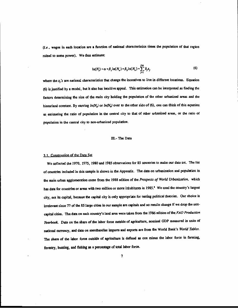
(i.e.. wages In each location are $ function of national characteristics times the population of that region

raised to some power). We thus estimate:

ln(N) =a+$1ln()+$2ln()+ES,1, (6)

where the i/s are national characteristics that change the incentives to Live in different locations. Equation

(6) is justified by a model, but it also has intuitive appeal. This estimation can be interpreted as finding the

factors determining the size of the main city holding the population of the other urbanized areas and the

hinterland constant. By moving ln(N_) or ln(N,) over to the other side of (6), one can think of this equation

as estimating the ratio of population in the central city to that of other urbanized areas, or the ratio of

population in the central city to non-urbanized population.

ilL-The Data

3.1. Constnictionof the Data Set

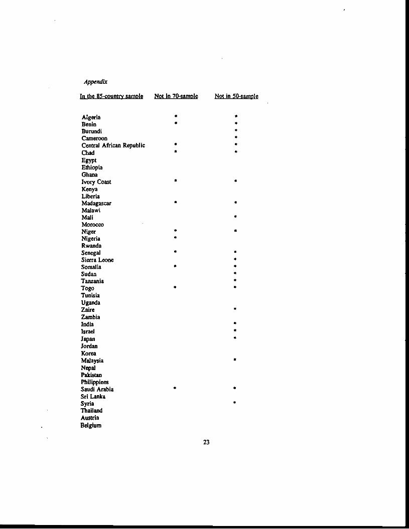
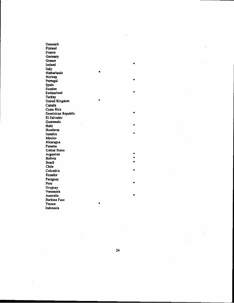
We collected the 1970, 1975, 1980 and 1985 observations for 85 countries to make our data set. The list

of countries included in this sample is shown in the Appendix. The data on urbanization and population in

the main urban agglomeration come from the 1988 edition of the Prospects of World Urbanization, which

has data for countries or areas with two million or more inhabitants in 1985.' We used the country's largest

city, not its capital, because the capital city is only appropriate for testing political theories. Our choice is

Irrelevant since 77 of the 85 large cities In our sample are capitals and no results change If we drop the non-

capital cities. The data on each county's land area were taken from the 1986 edition of the F4O Production

YearbooE Data on the share of the labor force outside of agriculture, nominal GDP measured in units of

national currency, and data on merchandise imports and exports are from the World Bank's World Tables.

The share of the labor force outside of agriculture is defined as one minus the labor force in farming,

forestry, hunting, and fishing as a pacentage of total labor force.

7

Data on total population, political rights and Instability are from the Barro and Wolf 11989) database.

GDP numbers are compiled by Summers and Heston [1991). The Gastil index of political rights annually

ranks countries in seven categories according to a checklist of political rights. The data on political

instability measures the number of revolutions, coups or strikes per year in each country. The data on

Import duties and government expenditures on transportation and communications are from the flff's

Cowniment FThance Swilsiles.

Our basic sample has 85 countries, but we lose several observations in dealing with import duties and

government transportation expenditures. We used averages of the 1970, 1975, 1980and 1985 observations

when feasible except thr the data directly taken from the Barro-WoIf data set?

3.2. Descriotion of the Data

The 1988 Prospects of World Urbanlzo4on reports 100 urban agglomerations with 2 million or more

Inhabitants in 1985 (compared to 62 in 1970). Thesecities account for 487 million inhabitants, wbich

represents 10 percent of the world's total population and 24 percent of the world's urban population. Of

those 100 largest urban agglomerations, 40 are in the more developed regions of the world. In 1985, 46 of

them contained between 2 and 2.9 million persons, 24 containS between 3.0 and 4.9 million, and 30 had

more than S million inhabitants. In this last group, eleven agglomerations contained 10 million or more

persons, with 7 of them in the less developed regions of the world. During the 15-year period of 1970-85

that we analyze, agglomerations that in 1985 had 2 million or more inhabitants grew faster than the world's

total population. While large agglomerations in the developed world grew at an average of 1.0 percent per

year, their counterparts in the less developed world grew at an average rate of 3.3 percent per year.

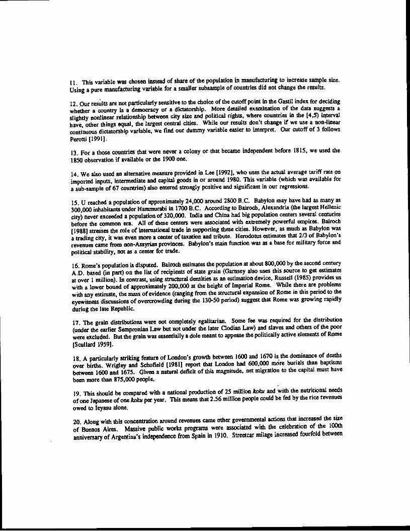
Table I shows the five largest and five smallest main cities of the world first ranked by absolute population

and then ranked by share of their country's population. Ranking by either measure, three of the five largest

main cities in the world are in less developed countries. Ml of the smaller cities are in less developed

countries. The correlation between absolute population and share of country's population is far from perfect.

8

Shanghai is one of the world's most populated main cities when ranked by its raw population and one oldie

world's teat populated main cities when ranked by its share of China's population. The southern cone of

South America seems particularly prone to urban concentration; three of the five most concentrated countries

in the world are there.

IV.- Results

Table II gives the means and standard deviations for the sample that we use in our regressions. Table

III shows the raw correlations of our variables. Higher levels of central city population were positively

associated with larger and more populated countries, high levels of per capita GOP, and high shares of the

labor thrce outside of agriculture. Central city population is negatively correlated with the presence of

dictatorships, the share of trade in GOP, and the share of government transportation and communication

expenditures in GDP. The growth rate of main city population Is positively associated with dictatorships.

revolutions and coups, and high tariff barriers. The correlations also show a strong correlation between

trade and politics which creates the possibility that trade and political effects might be confused empirically.

We use the log of average population in the main city as the dependent variable in most of our regressions.

MI regressions include the same set of controls: a capital city dummy that takes a value oft if the main city

in question is a capital city and 0 otherwise, the log of average non-urbanized population, the log of average

urbanized populatioi outside of the main city, the log of average real per capita GDP, and the log of land

area. Unless otherwise specified, all of our regressions report OLS results,with standard errors based on

White's heteroskedasticlty-cOnsisteflt covarlance matrix In parenthese&'°

Regression (I) includes our standard set of controls and the share of the labor force outside of agriculture.

The regression explains 80 percent of the total variation in the dependent variable. In regression (1),the

capital city dummy is positive and significant. The coefficient ott this variable indicates that main cities are,

on average, 42 percent larger if they are also capital cities. This faa may mean that power attracts

9

population, but It may also mean that capitals are located In larger cities. Bothpopulation controls also take

positive values, but only the log of non-urbanized population is large and significant. This coefficient is

typically well below one so that urban areas grow with their countries but less than proportionately. The

coefficient on the log of land area is also positive and usually close to 0.12, implying that a 10 per cent

increase in the size of the country increases population in the main city by about 1.2 per cent. The size of

the country (holding population constant) is a decrease in population density which might mean an increase

in the transportation costs of supplying the hinterland. This result provides our first support for the Kruginan

hypothesis.

Our income control usually takes positive values, but the coefficient loses size and significance whenever

we also control for the share of labor outside of agriculture. The share of labor outside agriculture is meant

to capture the country's state of industrial development and the fraction of the population that is not tied to

natural resources." This last variable has a large and significant effect on the size of the main city. We

find that a I percent increase in the share of the labor force outside of agriculture increases the size of the

largest city by about 2.5 percent. The agriculture and GD? results both suggest that large cities require

sonic economic development.

Regression (2) adds the share of trade in GD? to our first regression. This variable is negatively related

to the size of the largest city. An increase of 10 percent in the share of trade in GDP leads to a reduction

of 6 percent in the size of the main city. Alternatively, a one standard deviation increase in the share of

trade in GD? reduces the size of the main city by about 13 percent. This result supports Krugtnan and

Livas' [1992J theory against the alternative hypothesis that big cities grow as a result of commerce and trade.

The third regression in Table IV shows our first political variable. This dictatorship dummy (hased on

Gastil's indexes of political rights) assigns a value of 1 to countries who do not protect of political rights.

Since our predictions about dictatorship occur because dictatorships ignore the political rights of their

citizens, this measure is good for our purposes. Adding this dictatorship dummy to our list of controls, we

find that dictatorships have main cities that are about 45 percent larger than those belonging to countries with

10

non-dictatorial regimes? We deal with the possible endogeneity of the trade an4 dictatorship variables in

Tables VI and VII.

Region dummies are generally excluded from our regressions because we want to include the information

contained In interregional variation, but to check robustness we include region dummies in regression (4).

Our three main variables of interest remain significant and large, although the coefficients on trade and

politics fall by about a quarter. The coefficient on the Latin American dummy is positive and indicates that

countries in this region have main cities that are 40 percent larger than those of other countries.

In regression (5) we add a second political variable to regression (4). The New Democracy dummy was

constructed using data from Banks (19731, which contains data fOr a wide cross-section of countries going

back to 1815. This variable takes a value of I if the country in question did not have a well functioning and

efficient Parliament at the time it became independent, but was democracy between 1970 and 1985." This

New Democracy Dummy is intended to capture the effect of political history on the size of the central city.

Regression (5) shows that among the democracies in our sample, those that were dictatorships in the past

have central cities that are 40 percent larger than those of countries that were always democracies.

The final regression in Table W Includes the average number of revolutions and coups as a regressor, and

an Interaction between this variable and the dictatorship dummy to the previous set of regressors. We find

that political instability substantially increases city size in democracies. In those regimes, one extra

revolution or coup per year increases the average size of the central city by 2.4 percent. In dictatorial

regimes political Instability does not change the main city size.

The first three regressions in Table V examine the trade-city size connection more closely. Regression

(7) includes a tariff variable: the ratio of import duties to total imports." We find that import duties do

indeed expand the size of the primary city. A one percent increase in the ratio of import duties to imports

raises the size of the central city by almost three percent. The import duty effect remains important when

we control fOr the quantity of trade and dictatorship in regressions (8) and (9)..

Regress Ion (10) includes the share of government expenditures spent on transportation and communications

11

for a small subset of our sample (50 countries). A one percent increase in the share of ODP spent on

government transportation expenditures reduces main city size by 10 percent. This evidence supports

Krugmafl 119911: high internal transport costs create an Incentive for the concentration of economic activity

In space. Regression (ii) further examines the role of transportation costs using the density of roads in 1970

(from Canning and Pay [19931). The coefficient on the initial density of roads in the country is negative

(and the coefficient on government spending stays negative), further indicating that well developed transport

facilities lower the size of central cities; The last regression in Table V controls for possibly omitted

political effects and shows that the transportation expenditures are robust to controlling for political effects.

Tests for Causality

Like most of our variables, transport spending is endogenous. Similar caveats apply to our trade and

dictatorship variables. Concentration of population in a single city might give local finns a transport cost

advantage over foreign suppliers and thus lower the amount of foreign trade. Dictator's coups might be

easier in spatially concentrated countries

To examine the results of Table IV more closely, Table VI reproduces regression (5), but allows for the

possibility that trade and the dictatorship dummy are endogenously determined. We use three sets of

instruments to examine how exogenous changes in the share of trade in GDP and the type of political regime

alter the size of the main city:

(1) Regional Political Characteristics: Following Ades and Chua (1993) we use the average number of

revolutions and coups in neighboring countries, the average number of per capita political assassinations in

neighboring countries, and a dummy variable that takes a value of 1 if the average Gastil index of political

rights in neighboring countries is higher than 3.

(2) Predetennined Political Characteristics: We use the 1960 value of an index of etluiolinguistic

fractionalization in the country (from Taylor and Hudson 119721 as in Alesina and Rodrik (1993]), and a

dummy variable that takes a value of I if the country became independent after the end of World War fl.

12

T

(3) Regional Infrastructure: we use the average road density in neighboring countries (from Canning and

Fay 11993]).

Our Identifying assumptions are that these variables affect politics and trade but do not change urban

structure directly. We test these assumptions using a Wu-Hausman test of the overidentifying restrictions

for the system of equations and find that our assumptions pass these tests.

Regression (13) repeats regression (5) using our instrumental variables approach. The coefficient on the

dictatorship dummy remains significant and large. A one percent increase in the probability of having a

dictatorship increases the size of the central city by about 1.8 percent. The coefficient on the share of trade

in (3DP is negative and smaller than the estimates obtained with OLS. Regression (14) add to our list of

instruments the fitted valueS obtained from running a PROBIT for the Dictatorship Dummy and a TOBIT

for the Share of Trade on all the exogenous variables in the system. This specification improves the

precision of the first stage regression by improving the functional form. The coefficient on the dictatorship

dummy now falls to a level consistent with our previous OLS estimates. The coefficient on trade, while

negative and large, is still not estimated precisely.

Instrumental variables provide one approach to causality. Timing provides another approach. The first

three regressions in Table VII examine causality using the correlation of initial variables with later changes.

This test for causality is imperfrct, but at least we can see whether large central cities push countries into

dictatorship or whether dictatorships expand central cities. The timing of the relationship between country

variables and urban concentration shows what predates what Of not what causes what).

Regression (15) looks at the effect of the spatial distribution of population on the change in the share of

trade in GDP. We find no effect of main city size on trade growth. In regression (16), the dependent

variable becomes the dictatorship dummy for 1985, controlling for the dictatorship dummy In 1970. This

regression captures the effect of initial urban concentration on the probability of being a dictatorship in 1985,

conditional on being a dictatorship In 1970. We find no evidence for large central cities causing a switch

13

to dictatorship or preventing a switch away from dictatorship. Regression (17) makes the growth rate of

population in the main city between 1970 and 1985 the dependent variable. The role of dictatorships here

is critical: the presence of a dictatorship increased the growth rate of population in the main city by 1.3

percent a year. Trade has a weak or nonexistent effect.

RegressIon (18) suggests that concentration in a single city also ha strong negative effects on growth.

A Ipercent increase In the share of total population living in the central city reduces the growth rate by 0.08

percent per year. Large cities generate rent seeking and instability, not long term economic growth.

The results of this section support the idea that dictatorship causes urban centralization. Tests based on

instrumental variables and on the timing of growth both indicate that dictatorship influences urban

development. Our evidence does not confirm any causal relationship between trade and city size.

VI. Short Case Studies

6.1. Rome. 50 B.C.

At it's height, Rome's population probably stood at over 1,000,000 inhabitants, or approximately 2 percent

of the Roman empire's population. Earlier cities had been large but none had never grown to one half that

size.'3 There is dispute over Rome's population. In this discussion we accept Garnsey's 119881 population

figures and his claim that 130-30 B.C.E., when Rome's population grew from 375,000 to 1,000,000, was

the period of Rome's greatest growth.1' During this time, five distinct political events directly and

indirectly increased the incentives to come to Rome: (I) the empire expanded into Gaul and the eastern

provinces of Asia, Bithynia, Pontus, Cilicia and Syria, (2) Pompey declared that all conquered land was the

property of the city's government, (3) the Gracchi's Sempronian law and then the Clodian law extended the

grain distribution to a large number of the citizens as long as they me to Rome, (4) Sulla extended the

Roman citizenship to all of the inhabitants of Italy, and (5) internecine warfare made the hinterland

Aindamentally unsafe. As a result of events (3) and (4), by 46 B.C.E. 320,000 people were in Rome

14

receiving grain handouts.

The first two events mentioned above were the result ofsuccessful Roman military leadership, impressive

technology and the remarkable incentives (ranging from great wealth to control over the world's largest

empire) offered to reward military success. Events (3X5)are related to internal Roman weakness. The

traditional aristocracy was forced during this period, first by the Gracchis and later by popular uprisings,

to distribute grain more liberally to Roman citizens.'7 The expansion of citizenship throughout the Italian

peninsula was the result of the Roman failure (under the leadership of Gaius Marius) to reject the demands

of the Italian rebels in 90 B.C.E., despite these rebels' defeat in the Social Wars. Weak governmental

control over local mobs and strong control over distant empires, enabled Roman mobs to extract rents

(indirectly via the legions) from distant Egypt and Spain. The Roman empire delivered rents not just to the

Proconsuls of the territories but also to thegeneral population of the capital. Most visible of all these rents

transferred from the conquered provinces to the masses of Rome were the circuses (and other games) which

cost fortunes to produce Intl were put on at their height more than 50 times per 'ear.

Eventually, Julius Caeser restored stability and reduced the grain distribution around 45 B.C.E. The

growth of Rome then began to slow. Rome's growth illustrates how an ability to extract from the hinterland

and an inability to quell revolts at borne, together lead towards overconcentration in the capital. Trade and

industry may bave helped Rome expand, but Rome's huge unemployment levels, the overwhelming size of

the stat&s bureaucracy and the massive wealth redistributions make it clear that Rome's size was, ultimately,

a result of governmental size and transfers. The timing of Rome's expansion suggests that liberal grain

distributions funded by foreign conquests fueled Rome's growth.

6.2. London 1670. A. D.

For almost 1200 years after Rome's disintegration in the fifth century C.E., Europe had only two cites

with 400,000 or more inhabitants: Byzantium, with a population of bdween 400,000 and 600,000 from

600-1000 C.E., and Cordoba with a population of approximately 400,000 in 1000 C.E. [Bairoch 1988J.

15

The first strictly European metropolises to come close to 500,000 inhabitants were London and Paris around

1700. While the first British population census with data for London is In 1801 (giving London a population

of 960,000), Wrigley (19861 has earlier estimates that seem consistent with the numbers given by Bairoch,

Braudel and others. His estimates for London's population are 55,000 in 1520 (or 2.25 percent of England's

population), 200,000 in 1600 (or 5 percent) and 475,000 in 1670 (or 9.5 percent). London's population

continued to rise after 1670, and as a share of England's population it peaked at 11 percent in 1700."

While the rise of textile production In London in the late 16th century did coincide with the period of the

city's growth, London's rising control over these goods indicates more about the increasing importance of

trade than about any causal role played by textile technology. The rise in trade is one explanation of

London's growth. The late 16th century saw innovations in both internal and external trade. Kerridge

119881 argues that the ur-whS cart (a major innovation introduced in 1558) made transport much cheaper

within England and increased London's role as a center of internal commerce. International trade grew

because of military victories against the Spanish, improvement in shipping technology, the discovery of vast

new markets in Asia and the Americas and rising government support r trade. The London transport

industry also benefitted from the massive emigration to the New World [Borer 19771.

Some of the trade related factors were actually political. The ability of England to subdue Spain, the

emigration to British colonies, and large trade reflects in part political strength abroad. The allocation of

rents to local trade monopolies represents Stuart weakness at home. London's' growth was also closely

related to political factors such as the centralization of Tudor and Stuart power. Despite the unusual English

system of local justice, the centralization of military power and financial strength in the hands of Parliament

and the King in the city of London made England the European nation with the most centralized political

stnicture and the most control over its provinces (Brewer [19901).

Several Thdor monarchs (Henry VII, Henry VIII and Elizabeth I) were strong, but the Stuarts (James I

and Charles I), who ruled during the period of London's greatest growth, were England's most dictatorial

kings and had a particular disregard for the rights of the hinterland supposedly protected by parliament.

16

Smart instability is also easily seen; Charles I lost his thrown and his head in the Civil War. As in our

model, these dictators responded to Instability by collecting more income from the weak provincial areas and

relatively less from the dangerous capital. Examples of Stuart redistribution from provinces to capital

include James l's novel imposition of naval taxes (ship moneys) on the hinterland. James I also recreated

trade monopolies (which had been eliminated by Elizabeth I) and allocated them to the great London

merchants. Stuart mercantilisni can be seen as a policy enriching the capital's traders and producers at the

expense of the hinterland's consumers (Ekelund and Tollison 1981]. Instability also increased London's size

because the mid-l7th century civil war made much of the hinterland unsafe. It is unclear if London's growTh

was more strongly based on trade or politics, but we believe that the evidence points to the importance of

both factors.

6.3. Edo. 1700 A. D.

While both Paris and London appeared like colossi upon the map of Europe in 1700, neither city was

nearly as big as the Asian capitals of China and Japan. Peking had reached a population of 600,000 by

1500, and was the largest city in the world until London surpassed it in 1830. Japan's capital, Edo (modem

Tokyo) was almost as large as Peking around 1700 in absolute terms and much larger when viewed relative

to Japan's much smaller population. Excluding military personnel. Edo's population lies between 500,000

(Sansom 19631 to I million (Seidensticker 1980J, or between 2 and 4 percent of Japan's population. The

high productivity of rice economies has been the traditional explanation of Asian urbanization, but while this

nutritional edge might explain urbanization in general, it does not explain its concentration in a single city.

The period of Edo's greatest growth was between 1380, when Edo was a castle surrounded by a village,

and 1700, when it became the second largest city in the world. Edo's growth derives from its establishment

as the Shogunal capital by Tokugawa leyasu. Ieyasu (along with Odo Nobun4a and Hideyoshi) unified

Japan in the late 16th century. Over the 17th century, Ieyasu's descendants amassed a monopoly of political

and economic power far beyond that of any European king. By 1690, the Shogun had rice revenues of 14.68

17

kob, approximately half of the country's produces and more than six times the Shogun's revenues In

1598." The Tokugawa shoguns stripped rival chieftains of their authority and limited the power of the

samurai (following the path of Hideyoshi and his great sword hunt). At the end of the civil war, 100,000

ronin (unemployed soldiers) were left lordless; many of these were induced to come to the military capital.

The dalmyo (local lords) and the shogunate cut soldiers off from their local power bases and encouraged

samurai to take their feudal dues as annuities and move elsewhere (mainly to the capital (Sansom 1963J).

Despite the power of the Shogun, some instability (such as the Shimabara uprisings of 1638-39) remained

In the hinterland and further encouraged people to move to the safety of the capital.

There is some support for die Knigman-Livas trade hypothesis In the story of Edo. The Tokugawa

shoguns excluded Christians from Japan in 1638. lowered the importance of foreign trade and thus damaged

Edo's rival, the international trade center of Nagasaki. Anti-commercial attitudes of the Baazfu (the

Shogunate) also limited the rise of Osaka (the leading commercial center). The anti-industrial bias of the

leadership further prevented any other cities growing from the development of local industries. Japan does

not display the Roman combination of strength abroad and weakness in the capital - the Shogunate was

strong everywhere. However, the sheer power of the central Japanese government created such a

disproportionate amount of employment, safety and wealth in Edo that It city became an urban giant.

6.4. Buenos Aires. 1900. A. D.

Latin American nations, such as Chile, Mexico, Peru and Uruguay, are often heavily concentrated in their

central cities. The first of these Latin American urban giants was Buenos Aires. By 1914, Buenos Aires was

the largest urban agglomeration south of the Hudson river with 1.6 million inhabitants (20% of Argentina's

population). Although Buenos Aires had been growing for 250 years before 1887 (and has not stopped

during the 80 years since 1914), the 27 years between 1887 and 1914 mark the period when the city grew

most. Over those 25 years, the city grew by more than 1.1 million people (an increase of 265 percent).

Industry did not play a prominent role in the rise of Buenos Aires. In 1914, less then 15 percent of

18

Argentine labor force was involved in manufacturing activities. The Argentine government displayed

hostility towards manufacturing and innovation (examples Include heavy tariffs on manufactured exports and

the absence of effective patent protection). By comparison, trade expanded heavily over this period. Total

exports rose 4(X) percent between 2887 and 1914 (measured in gold pesos, cattle or sheep). Approximately

20 percent of Argentina's population (and a much higher percentage of Buenos Aires' population) was

involved in commercial activities.

The growth of Buenos Aires came from Its role as a commercial center and from its role as a center for

migration. The city expanded with an almost even increase in native population and immigrants. The share

of immigrants (mostly of Italian and Spanish origin) in Buenos Aires' population was 52.4 percent in 1887

and 49.6 percent in 1914. From 1905 to 1909, immigrants to Argentina, almost entirely passing through

Buenos Aires, totalled around I million. Between 2887 and 1914, approximately 550,000 of the almost 3

million Immigrants to Argentina stayed In Buenos Aires. Buenos Aires retained a larger proportion of its

immigrants than its new world rival, New York, possibly because of (1) undeveloped transportation facilities

within the hinterland, (2) the absence of any other important pre-existing urban centers or industry in the

hinterland, (3) a decline in the demand for labor in the hinterland as agriculture was consolidated into large

firms that replaced labor with capital, and (4) instability in the hinterland coming from wars and unfriendly

relations with the native Americans.

Politics also played a role in Buenos Aires' growth. In 1914, 95 percent of the government's revenues

came from tariffs. Scobie 119141 suggests that this heavy dependence on port related income induced the

government to keep its activities in Buenos Aires, the source of its wealth. The heavy dependence on tariffs

also created an incentive for the government to support trade, and Buenos Aires, at the expense of industry

and the hinterland. The large share of government revenues that came from with also created a stunning

array of regulations open to interpretation by local officials. Not surprisingly, this created tremendous

opportunities for bribery or coima. An estimate by Scobie puts bribery in Argentina at about 25 percent of

government revenues. This kind of personalized corruption greatly increased the need to be close to the

19

officials administering the tariffs? Like London, Buenos Aires was a center for international movements

of goods and capital (both human and physical), but the concentration of government and bureaucratic

corruption also playeda prominent role.

6.5. Mexico City. Today

Mexico City (née Tenoebtitlan) dates from the 14th and 15th centuries, when it was built as the center for

the Aztec empire. Both the Aztecs and later the Spaniard extracted as much wealth as possible from

surrounding provinces and spent that wealth either in the city or sent it elsewhere (i.e. Spain). Despite a

limited role as a center for trade (e.g. the Manila Galleons), pre-modern Mexico was ultimately a collector

of rents. Mexico City remained a small rent-seeking capital until after World War 11. In 1900, when

Buenos Aires had already reached preeminence, Mexico City had 470,000 inhabitants. By 1940, the city

had 1.5 million people. By 1970, this number had swelled to 8.5 million (in the metropolitan area) and

today Mexico City's population has reached 18 million.

As Krugman and Livas argue, trade did not play a role in the growth of Mexico City; the city grew as

a center for manufacturing. Mexico's industrial expansion was heady in the 1945-1970 period. Industrial

real wages increased by 250 percent over this period. Manufacturing employment expanded by 2.3 million

(120 percent). The federal district's (Mexico City and its environs) share of manufacturing employment to

grow from 25 percent in 1950 to over 40 percent in 1960 and back down to 30 percent in 1970.

Employment in the service sector expanded by 1.2 million (600 percent). Agricultural employment actually

declined over the 1960-1970 period.

Industrial growth was concentrated in Mexico City because the capital was the major market for most

goods as well as the major supplier (Krugman and Livas's thesis). Mexico's industrialization followed the

big push type pattern [Murphy, Shleifer and Vishny 19891; urban concentration facilitated the coordination

of demand and supply. Import-substitution policies made it more necessary for consumers (especially firms

consuming intermediate inputs) to locate in Mexico city close to domestic suppliers because foreign suppliers

20

were excluded from the country. Industrial growth also thrived in the capital because Mexico City was the

center for foreign capital and ideas.

Political factors behind Mexico's concentration are also quite strong. Mexico has a nominally federal

government, but all real power Is concentrated In the capital. Even regional governors spend most of their

time within the capital out of fear of losing political Influence [Kandell 1988]. The Mexican government is

also particularly susceptibleto unrest in the capital. Kandell [1988] describes a typical episodeof rural-urban

migrants coming to the outskirts of the central city and beginning as squatters on the land. These migrants

then choose a political leader or cac1que who agitates against the leading party (the PR!). The government

responds by giving the migrants title to the land and providing them with some kind of minimal

infrastructure (paid for with taxes levied on the country as a whole). The migrants then become loyal

supporters of the PR!. This description of an oligarchic regime paying off local rioters with transfers seized

from remote regions of the country is highly reminiscent of Rome. It suggests that politics, as well as trade,

contributed to Mexico City's size.

VI!. Conclusion

Krugman and Llvas' (1992] hypothesis that urban concentration Is negatively related to international trade

is born out in the data. Good Internal transportation infrastructure also decreases urban concentration.

However, our time series and Instrumental variables results cast doubt on the causality in these correlations.

Trade and cities are connected, but it may be that urban concentration is causing low levels of trade, not that

low levels of trade induce concentration.

Our political results are stronger than our results on trade. They display a robust causality running from

dictatorship to urban centralization. Urban giants ultimately stem from the concentration of power in the

hands of a small cadre of agents living in the capital. This power allows the leaders to extract wealth out

of the hinterland and distribute it in the capital. Migrants come to the city because of the demand created

21

by the concentration of wealth, the desire to influence the leadership, the transfers given by the leadership

to quell local unrest and the safy of the capital. This pattern was true in Rome, 50 B.C., and ills true in

many countries today.

22

Appendix

In the 85-country samnie Not In 70-samnie Not in 50-samnle

Algeria * *Benin * *BurundiCameron *Central African Republic * *Chad *

EgyptEthiopiaGhanaIvory Coast * *

KenyaLiberiaMadagascar

* *MalawiMaiiMoroccoNiger * *

Nigeria *

Rwanda

Senegal* *

Sierra Leone *

Somalia *

Sudan *Tanzania *

Togo*

TunisiaUgandaZalit *ZambiaIndia *Israel *

Japan*

JordanKorea

Malaysia *

NepalPakistanPhilippinesSaudi Arabia * S

Sri LankaSyria *

ThailandAustriaBelgium

23

DenmarkFinlandFranceGermanyGreeceIrelandItalyNetherlands *

NorwayPortugal

*

SpainSwedenSwitzerland *

TurkeyUnited KingdomCanadaCosta RicaDominican RepublicEl SalvadorGuatemalaHaitiHondurasJamaica *

MexicoNicaraguaPanamaUnited StatesArgentinaBoliviaBrazil *

ChileColombiaEcuadorParaguayPeniUruguayVenezuelaAustraliaBurkina FasoYemenIndonesia

24

References

Ades, A. and H. Cbua, 'Thy Neighbor's Curse: Regional Instability andEconomic Growth,' Harvard mimeo, 1993.

Alesina, A. and R. Perotti, 'Income Distribution, Political Instability and Investment,'Harvard mimeo, 1993.

Bairoch, P., Cities and Economic Develoonient, Chicago: University of Chicago Press, 1988.

Barro, R., 'Economic Growth in a Cross-Section of Countries,' Ouaiterlv Journalof Economics 106: 407-444, 1991.

________ and H. Wolf, 'Data for Economic Growth in a Cross-Section of Countries,' NBER workingpaper, 1989.

Bollen, Kenneth A. 'Political Democracy: Conceptual and Measurement Traps,'Studies in Cotnoarative Innational Develonment 25: 7-24, 1990.

Borer. M., The City of London, London, Constable, 1977.

Braudel, F., Civilization and Canitalisin. New York: Harper & Row, 1979.

Brewer, 0., The Sinews of Power, Cambridge, Harvard University Press, 1990.

Canning, D. and M. Pay, 'The Effect of Transportation Networks on Economic Growth,iscussion Paper,Columbia University, 1993.

beLong, B. and A. Sbleifer, 'Princes and Merchants: European City Growth before the IndustrialRevolution,' Journal of Law and Economics. 1993.

Ekelund, R. and R. Tollison, Mercantilism as a Rent-Seetins Society, College Station: Texas A & MUniversity Press, 1981.

Garnsey, P., Famine 2nd Food Sunnlv in the Graeco-Roman Work!, Cambridge: Cambridge UniversityPress, 1988.

Gastil, R. Freedom in the World. Westport: Greenwood Press, 1987.

Glaeser, E. L., H. D. Kallal, J. A. Scbeinkman, and A. Shleifer, 'Growth in Cities,' Journal of PoliticalEuinomv. vol.100, no.6, 1992.

Henderson, J. V., Economic 'Theory and the Cities, New York: Academic Press, 1986a.

Hoselitz, B., 'Generative and Parasitic Cities,' Economic Develootnent and Cultural Cbajwe 3: 278-294,1955.

Kandell, I., l.a Canital: The Biogranhv of Mexico City. New York, Henry Molt, 1988.

25

Kerridge, E., Trade and Banking in Early Modern Entland, Manchester: Manchester University Press,1988.

Krugman, P., 'Increasing Returns and Economic Geography,' Journal of Political Economy 99: 483499,1991.

______ and R. Livas, "Trade Policy and the Third World Metropolis', NBER working paper #4238,1992.

Lee, J-W., 'International Trade, Distortions and Long-Run Economic Growth,' Harvard Universitymimeo, 1992.

Mominsen, T., The History of Rome. New York, Meridien Books, 1958.

Murphy, K., A. Shleifer and It. Vishny, "Industrialization and the Big PUSh,'Journal of Political Economy97: 1003-1026, 1989.

Nash, (I. B., 'The Urban Crucible: The Northern Seanorts and the Origins of the American Revolution,Cambridge: Harvard University Press, 1986.

Olson, Mancur, The Rise and Decline of Nations: Economic Growth. Starnation and Social RiSities, YaleUniversity Press, 1982.

Perotti, Roberto, 'Income Distribution and Growth: Theory and Evidence," mimeographed, 1991.

Rosen, K. and M. Resnick, 'The size distribution of cities: an examination of the Pareto Law and Primacy,'Journal of Urban Economics 8, 1980.

Russell,). C., Late Ancient and Medieval Pooulation Control, Philadelphia, American Philosophical Society,1985.

Sansom, Sir George Bailey, A History of Janan, Stanford: Stanford University Press, 1963.

Scobie, James, Buenos Aires: Ptaza to Suburb. 1870-1910, New York, Oxford University Press, 1974.

Scullard, H.H., From the Graccbj to Nero: A History of Rome 133 BC to AD6Z, London: Routledge, 1959.

Seidensticker, E., Low City. High Cliv: Tokyo from Edo to the Great Earthouake, New York: Knopf, 1981.

Stiglitz, Joseph. E., 'Economic Organization,' in HolDs Chenery and T. N. Sr'mivasan Eds, Handbook ofDevelooment Economics, Amsterdam: North-Holland, 1991.

Summers, Robs, and A. Heston, "The Penn World Table (Mark 5): An Expanded Set of InternationalComparisons, 1950-1988," Ouarterly Journal of Economics 106: 327-368, 1991.

Taylor, Charles L. and Michael C. Hudson, World Handbook of Political and Social Indicators, ICPSR, AnnArbor Ml, 1972.

Wheaton, W. and H. Shishido, 'Urban Concentration, Agglomeration Economies and the Level of Economic

26

Development," Ecoaoinlc Develooment and Cultural (lange 50: 17-30, 1981.

Williamson, Jeffrey. 0., "Migration and Urbanization," in HolDs Chewy and T. N. Srinivasan Eds.Handbook of Development Economics, Amsterdam: North-Holland, 1991.

Wrigley, E., "Urban Growth and Agricultural Change: England and the Continent in the Early ModernPeriod," in Rotberg and Rabb Eds., Ponulationand Economy, Cambridge, Cambridge UniversityPress, 1986.

______ and R. Schofield. The Ponulation Historyof England. 1541-1871: A Reconsnction, Cambridge,Harvard University Press, 1981.

von Thflnen, Johann Heinrich, The Isolated State, Hamburg: Perthes, 1826. English translation. Oxford:Pergamon, 1966.

27

1. These three authors' evidence differs from ours because of (1) their use of self-construcéed politicalvariables, (2) their emphasis on explicitly spatial O.e. degree of local spending or autonomy) institutions (welook at more basic features of governments), (3) their small sample size (less than forty) and restrictive timeperiod (Henderson uses only 19741976). In addition to this, endogeneity problems are much more seriousfor their political variables. As one measure of government centralization, these authors use the share of localgovernments In total government expenditures. This variable Is dearly a function of the distribution ofpopulation in space. A further difftrence with out work. is that we only look at the nation's largest city.This change was necessary to increase sample size.

2. The relationship between trade and concentration can be non-monotonic. When foods deteriorates rapidlyin transit, people must live near food supplies, as they did before the domestication of pack ninml5 (Bairoch11988]).

3. Protectionist policies might also encourage urban concentration by promoting the growth of import-competing activities which are dependent on essential inputs found only in the capital; central cities mightbe — places for avoiding tarifft (New York City and Buenos Aires were both centers of smuggling);finally, proximity to central government might be particularly important when exemptions to tariffs are beinghanded out or the spoils ofprotection are being distributed.

4. Hoselitz [1955] argued that there were a class of 'parasitic' cities involved In rent-seeking. Olson (1982]emphasizes the roleof government distribution policies in determining thesize of cities. He suggests thatthe capital will grow when transportation and communication networks are poorly developed in rural areas;this, he claims 'makes it more costly and difficult for those in rural areas to mobilize political power...'.Williamson (1991] gives an elegant description of the policies put in place transferring resources from thehinterland to the capital. Technically, these theories are all about the nation's capital not the nation's largestcity. Since the nation's largest city is its capital in more than 90% of the countries in our sample, we havedecided to gloss over this distinction.

5. We would get identical results if the degree of dictatorship measured the size of the rents to be allocatedand the degree of instability measured the ability of local political actors to access those rents.

6. Our results could be generalized to allow revolts starting in both areas as long as the capital has acomparative advantage in unseating the government.

7. Both probabilities are conditional on the other change of government not occurring.

8. An urban agglomeration is an area comprising a central city or cities surrounded by an urbanized area,and is dose to the U.S. definition of 'consolidated statistical metropolitan area.'

9. Averages were used rather than running all four observations as a panel, primarily because appropriatepanel techniques are only usable If we put some structure on how lagged values of county characteristicschange current urban concentration. We were unwilling to make the assumptions needed for that structure.

10. These standard errors do not differ greatly, however, from those obtained by OLS. We also triedrunning the regressions weighting them by population.

28

II. This variable was chosen instead ofshare of the population in manufacturing to increase sample size.

Using a pure manufacturing variable for a smaller subsample of countries did not change the results.

12. Our results are not particularly sensitive to the choice of the cutoff point in the Gastil index for decidingwhether a country Is a democracy or a dictatorship. More detailed examination of the data suggests a

slightly nonlinear relationship between city size and political rights, where countries in the [4,5) interval

have, other things equal, the largest central cities. Whileour results don't change if we use a non-linearcontinuous dictatorship variable, we find our dummy variable easier to interpret. Our cutoff of3 follows

Perotti (19911.

13. For a those countries that were never a colony or that became independent before 1815, we used the1850 observation if available or the 1900 one.

14. We also used an alternative measure provided in Lee 119921, who uses the actual average tariff rate onimported inputs, intermediate and capital goods in or around 1980. This variable (which wasavailable for

a sub-sample of 67 countries) also entered strongly positive and significant in our regressions.

15. U reached a population of approximately 24,000 around 2800 B.C. Babylon may have had as many as300,000 inhabitants under Hammurabi in 1700 B.C. According to Bairoch, Alexandria (the largest Helleniccity) never exceeded a population of 320,000. India and China had big population centersseveral centuries

before the common era. All of these centers were associated with extremely powerful empires. Bairoch(19881 streises the role of international trade in supporting these cities. However, as much as Babylon was

a trading city, it was even more a center of taxation and tribute. Herodotus estimates that 213 of Babylon'srevenues caine from non-Assyrian provinces. Babylon's main function was as a basefur military force and

political stability, not as a center for trade.

16. Rome's population is disputed. Bairoch estimates the population at about 800,000 by the second centuryA.D. based (in part) on the list of recipients of state grain (Garnsey also uses this source to get estimatesat over I million). In contrast, using structural densities as an estimation device, Russell (1985) provides uswith a lower bound of approximately 200,000 at the height of Imperial Rome. While there are problemswith any estimate, the mass of evidence (ranging from the structural expansion of Rome in this period to theeyewitness discussions of overcrowding during the 130-50 period) suggest that Rome was growing rapidlyduring the late Republic.

17. The grain distributions were not completely egalitarian. Some fee was required for the distribution(under the earlier Sempronian Law but not under the later Clodian Law) and slavesand others of the poor

were excluded. But the grain was essentially a dole meant to appease the politically active elements of Rome

(Scullard 19591.

18. A particularly striking feature of London's growth between 1600 and 1670 is thedominance of deaths

over births. Wrigley and Schofield 119811 report that London had 600,000 more burials than baptismsbetween 1600 and 1675. Given a natural deficit of this magnitude, net migration to the capitalmust have

been more than 875,000 people.

19. This should be compared with a national production of 25 million koband with the nutritional needs

of one Japanese of one koku per year. This means that 2.56 million people could be fed by the rice revenues

owed to Ieyasu alone.

20. Along with this concentration around revenues caine other governmental actions that increased the size

of Buenos Aires. Massive public works programs were associated with the celebration of the loath

anniversary of Argentina's independence from Spain in 1910. Streetcar inilageincreased fourfold between

1887 and 1914. There was no corresponding increase public investment in the hinterland.

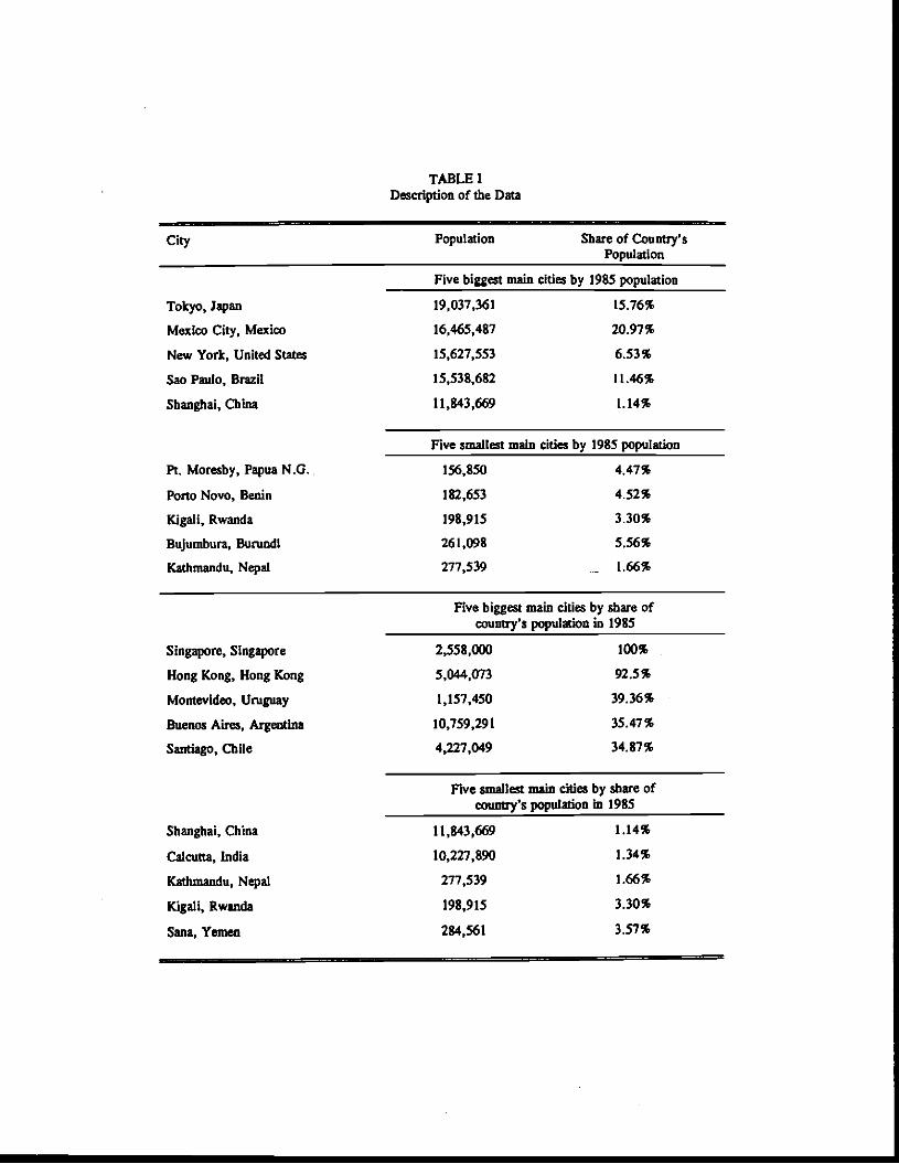
TABLE IDescription of the Data

City Population Share of Country aPopulation

Tokyo, Japan

Five biggest main cities by 1985 population

19,037,361 15.76%

Mexico City, Mexico 16,465,487 20.97%

New York, United States 15,627,553 6.53%

Sao Paulo, Brazil 15,538,682 11.46%

Shanghai, China

Pt. Moresby, Papua N.G.

11,843,669 1.14%

Five smallest main cities by 1985 population

156,850 4.47%

Porto Novo, Benin 182,653 4.52%

Kigali, Rwanda 198,915 3.30%

Bujumbura, Bunandi 261,098 5.56%

Kathmandu, Nepal 277,539 1.66%

Singapore, Singapore

Five biggest main cities by share ofcountry's population in 1985

2,558.000 100%

Hong Kong, Hong Kong 5,044,073 92.5%

Montevideo, Unsguay 1,157,450 39.36%

Buenos Aires, Argentina 10,759,29! 35.47%

Santiago, Chile 4,221,049 34.87%

Five smallest main cities by share of

Shanghai, China

country's population in 1985

11,843,669 1.14%

Calcutta, india 10,227,890 1.34%

Kathmandu, Nepal 277,539 1.66%

Kigali, Rwanda 198,915 3.30%

Sana, Yemen 284,561 3.57%

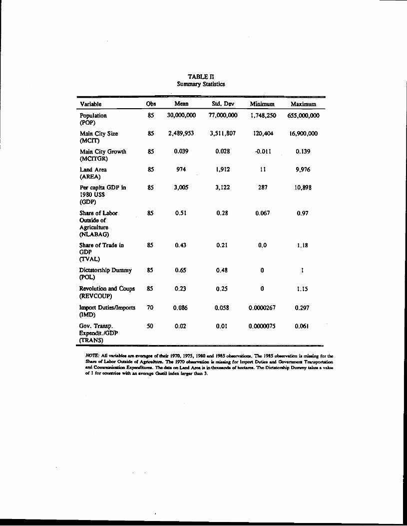
TABLE USummary Statistics

Variable Obs Mean SW. Dcv Minimum Maximum

Population(POP)

85 30,000,000 77,000,000 1,748,250 655,000,000

Main City Size(MCIT)

85 2,489,953 3,511,807 120,404 16,900,000

Main City Growth(MCITGR)

85 0.039 0.028 -0.011 0.139.

Land Area(AREA)

85 974 1,912 11 9,976

Per capita GDP In1980 USS(GDP)

85 3.005 3.122 287 10,898

Share of LaborOutside ofAgriculture(NLABAG)

85 0.51 0.28 0.067 0.97

Share of Trade inGDP(TVAL)

85 0.43 0.21 0.0 1.18

Dictatorship Dummy(POL)

85 0.65 0.48 0 1

Revolution and Coups(REVCOUP)

85 0.23 0.25 0 1.15

Import Duties/Imports(IMD)

70 0.086 0.058 0.0000267 0.297

Gov. Transp.Expend it./GD'P(TRAINS)

50 0.02 0.01 0.0000075 0.061

NOTh: All variable. an .va.ge. of their 1970, 197$, 1950 and 19*5 ob.avatio,. lIt 1915 observation ii missing for theSbszs of labor Outside of Agriculwn. The 1970 observsioe is missing (or Impoit Duties and Oovcnnad Tisaspoitationand C zhoa Expendhuna. The data mi Land A,e. ii in thousand. of beasm. The DictstoS.ip Dummy takes a vaijisof I for cowtie. with an avenge Onatil index larger than 3.

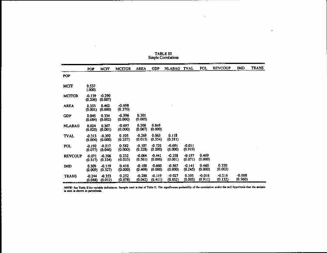
TABLE 111Simple Correlations

POP MCIT MCITGR AREA GDP. NLABAG TVAL POL REVCOUP 1Mb TRANS

Pop

MCIT 0.537(.000)

MCITGR -t139 -0.290(0.206) (0.007)

AREA 0.353 0.462 -0.098(0.001) (0.000) (0.370)

GDP 0.045 0.334 -0.596 0,301(0.684) (0.002) (0.000) (0.005)

NLABAG 0.024 0.367 -0.697 0.200 0.849(0.825) (0.001) (0.000) (0.067) (0.000)

TVAL -0.313 -0.392 0.105 -0.269 0.065 0.118(0.004) (0.000) (0.337) (0.013) (0.554) (0.28 1)

POL -0.192 -0.217 0.582 -0.107 -0.720 -0.691 -0.011(0.077) (0.046) (0.000) (0.328) (0.000) (0.000) (0.919)

REVCOUP -0,071 -0.106 0.232 -0.064 -0.44! -0.358 -0.197 0.469(0.517) (0.334) (0.033) (0.561) (0.000) (0.001) (0.071) (0.000)

IMD 0.309 -0.119 0.416 -0.100 -0.660 -0.567 -0.141 0.460 0.350(0.009) (0.327) (0.000) (0.408) (0.000) (0.000) (0.245) (0.000) (0.003)

TRANS -0.244 -0.353 0.252 -0.288 -0.119 -0.027 0.395 -0.016 -0.216 -0.008(0.088) (0.012) (0.078) (0.042) (0.411) (0.852) (0.005) (0.911) (0.132) (0.960)

Mfl See TabtaBlat vañabta delinitionL Sample u.ed I. that of Table tI The iigniftcanee prvbability of the correlation under the idI hypothesis that the ut.tSicis rmu is ihown in parenthesis.

TABLE IV

Dependent Variable: Log of AveragePopulation in Main CIty (1970-1985)

(1) (2) (3) (4) (5) (6)

Intercept 1.136(0.878)

2.014(0.934)

1.516(0.942)

0.651(1.109)

0.808(1.082)

0.297(1.063)

Capital City Dummy 0.424(0.204)

0.465(0.196)

0.374(0.181)

0.336(0.200)

0.283(0.180)

0.408(0.188)

Log of AverageNon-Urbanized Population

0.595(0.068)

0.553(0.066)

0.583(0.063)

0.640(0.073)

0.623(0.072)

0.641(0.071)

Log of Average UrbanizedPopulation Outside the Main City

0.059(0.050)

0.066(0.045)

0.063(0.042)

0.058(0.042)

0.054(0.040)

0.045(0.038)

LogofLand Area 0.161(0.051)

0.155

(0.049)0.115(0.049)

0.109(0.054)

0.113(0.053)

0.120(0.055)

Log of Average Real ODPper Capita

0.034(0.129)

0.058(0.131)

0.165(0.127)

0.193(0.146)

0.149(0.149)

0.166(0.148)

Average Share of the Labor ForceOutside of Agriculture

2.656(0.554)

2.556(0.567)

2.704

(0.549)2.623

(0.541)2.782

(0.518)3.071

(0.516)

Share of Trade in GDP -0.609

(0.225)

-0.676(0.204)

-0.463(0.228)

-0.404(0.240)

-0319(0.244)

Dictatorship Dummy Based onGastil's Index of Political Rights

0.444(0.154)

0.324(0.156)

0.442(0.148)

0.705(0.181)

Africa Dununy 0.160(0.263)

0.127(0.260)

0.172(0.257)

Latin America Dummy 0.390(0.159)

0.342

(0.158)

0.295(0.162)

New Democracy 0.428

(0.177)

Revolution and Coups 2.372(0.772)

Dictatorship Dummy *Revolution and Coups .

-2.705

(0.803)

Number of Observations 85 85 85 85 85 85

Adjusted R2 0.81 0.81 0.82 0.83 0.83 0.84

NO7E All vui.bk. are avenge, of their 1970. 1915. 1980 .nd 19*5 obsavaziona. The 19*5 obsention iamining for the Share or I.thor Outaide of Agriculture. The DictatoSdp Dummy take,. value of I for ooumrieswith an avenge Quell index larger than 3. White.conected atandazd toot. in pazat.eaia.

TABLE V

Dependent Variable: Log ofAvenge Population in Main

City (1970-1985)

(7) (8) (9) (10) (11) (12)

Intercept 3.015(0.927)

3.768(1.059)

3.128(0.992)

2.475(0.823)

2.2792(0.8010)

1.752(0.8224)

Dummy for Capital City 0.445(0.214)

0.460(0.209)

0.375(0.180)

0.566(0.244)

0.5190(0.2151)

0.4592(0.2146)

Log of AverageNon-Urbanized Population

0.491(0.075)

0.456(0.075)

0.498(0.072)

0.191

(0.112)

0.1547(0.1160)

0.2259(0.1064)

Log of Average Urbanized

Population Outside the Main

City

0.091(0.056)

0.097

(0.05!)0.092

(0.049)0.504

(0.110)0.6071

(0.1228)0.5312

(0.1154)

Log of Land Area 0.176(0.063)

0.262(0.060)

0.124(0.061)

0.115

(0.070)0.0039

(0.0778)0.0228

(0.0734)

Log of Average Real GDP perCapita

0.686(0.114)

0.676(0.112)

0.825

(0.129)0.217(0.129)

0.2478(0.1342)

0.4488(0,1418)

Import Duties/Imports 2.942(1.424)

2.909(1.415)

2.733(1.212)

Share of Trade in GDP .0.535(0.342)

.0.512(0.303)

Dictatorship Dummy Based onGastil's Index of PoliticalRights

0.444(0.177)

.

0.458(0.2206)

Share of GovernmentTransportation andCommunication Expendituresto ODP

-10.481(5.717)

-10.320(4.8250)

-8.624(4.293)

Roads Density in 1970 .0.00036(0.00016)

-0.00023(0.00015)

Number of Observations 70 70 70 50 50 50

Mjusted R3 0.77 0.78 0.79 0.84 0.85 0.86

Note: See Tale IV. The 2910 o4nezv.tion is mining (or Inipoit Dutia aM Oovcnund Truiapoxtstion aM ComnuiicstionExpeadituru.

TABLE VI

DopeDdent Variable: Log of AveragePopulation in Main City (1970-85)

(13)2SLS

(14)2SLS

Intercept -0.738(2.607)

1.919(1.512)

Dummy for Capital City 0.065(0.366)

0.383(0.233)

Log of Average Non-Urbanized 0.7 10 0.565Population (0.146) (0.086)

Log of Average Urbanized 0.047 0.066Population Outside the Main City (0.056) (0.042)

Log of Land Area 0.003(0.103)

0.051(0.03!)

Log of Average Real GDP per Capita 0.472(0.289)

0.194(0.175)

Share of Labor Outside of Agriculture 3.240(0.909)

2.672(0.638)

Share of Trade in GDP -0.361 -1.017.

(1.197) (0.857)

Dictatorship Dummy Based on 1.788 0.511Gastil's Index of Political Rights (0.901) (0.291)

Number of Observations 85 85

Adjusted Rt 0.69 0.82

85R2 of regression of -0.063 -0.02residuals on instruments

p-value of restrictions 0.75 0.75

?V7E: See Table IV. In ,egttaiom (13) and (14), tMDidatoS4 Dummy and the Share ofTrade in ODP an Unted — n.dogenou.. The inmn.marda Us we u.ed an the avenge swmbcrof ,evolution. and coup. in neighboring countka, the avenge ixunba of per capita politicalaa...ainalio.ia in neighboring eount,S, * dummy variable that take. a vahse of I if the avengeGaaS Index of political d5M. in neighboring ecwtrie. S higher than3 and 0cthetwiae. the1960 yak., of the dl.nie ogeneiy index, • dummy variable Us take. a value of liftSeowty bee..,. =t after the end of Woild War II and 0 otherwin, and IS avengemed den.ity in neighboring courSe. In regreion (14), we add twe geneated inMiutncfl. Inour lit of eortob: this axe the trued value. oasiss (torn amning a PROfIT for theDidalonhip Dummy end a TOBFr for the Share of Tied. on all the cangemiul variablea in theayteni. The p-value, for the let of Ure ovetidertifying intridion. are obtained by tuaning Sre.iduala from the aecoird sage regreaaion on .11 the brurrcra. The obtained R' uwkipliedby the .mmber of ob,e.vasiona is diatributed —'x' with) degna of freedom, when) ii Srnsmber of Insiumeta mimi the number of intnmncd variable..

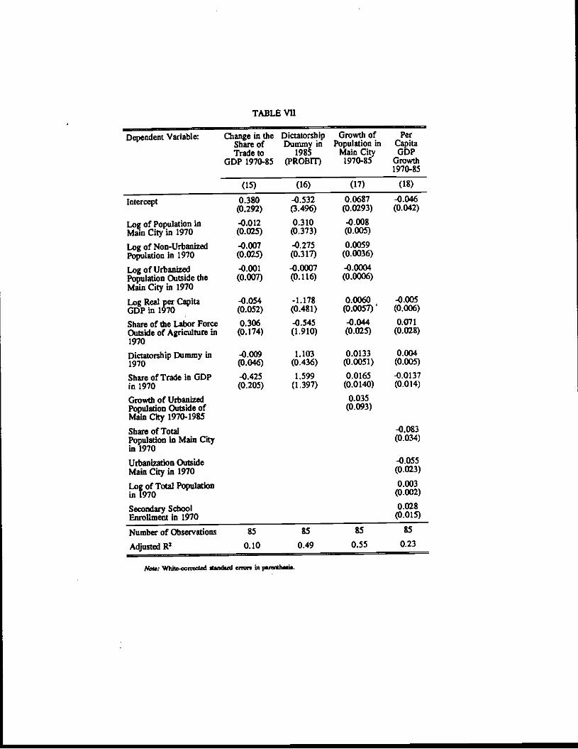
TABLE VII

Dependent Variable: Change in theShare ofTrade to

GDP 1970-85

DictatorshipDummy in

1985(PROBIT)

Growth ofPopulation in

Main City1970-85

PerCapitaGD?

Growth1970-85

(15) (16) (17) (IS)

Intercept 0.380(0.292)

-0.532(3.496)

0.0687).0293)

-0.046(0.042)

Lo of Population inMain City in 1970

-0.012(0.025)

0.310(0.373)

.0.008(0.005)

Log of Non-UrbanizedPopulation in 1970

.0.007(0.025)

-0.275(0.317)

0.0059(0.0036)

Log of UrbanizedPopulation Outside theMain City in 1970

-0.001(0.007)

-0.0007(0.116)

-0.0004(0.0006)

Log Real per CapitaGDP in 1970

-0.054(0.052)

-1.17$(0.48 1)

0.0060 -(0.0057)

.0.005(0.006)

Share of the Labor ForceOutside of Agriculture in1970

0.306(0.174)

-0.545(1.910)

-0.044(0.025)

0.071(0.028)

Dictatorship Dummy in1970

-0.009(0.046)

1.103(0.436)

0.0133(0.0051)

0.004(0.005)

Share of Trade In GD?in 1970

-0.425(0.205)

1.599(1.397)

0.0165(0.0140)

-0.0137(0.014)

Growth of UrbanizedPopulation Outside ofMain City 1970-1985

0.035(0.093)

Share of TotalPopulation in Main Cityin 1970

-0.083(0.034)

Urbanization OutsideMain City in 1970

-0.055(0.023)

Log ofTotal Populationin 1970

0.003(0.002)

Secondary SchoolEnrollment In 1970

0.028(0.015)

NumberofObservations 85 85 85 85

Adjusted R 0.10 0.49 0.55 0.23

Note: Wbito.con,dgd dazidstd enon in ptteshSt

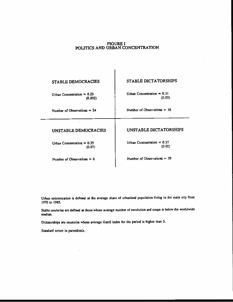
FIGURE IPOLITICS AND URBAN CONCENTRATION

STABLE DEMOCRACIES STABLE DICTATORSHIPS

Urban Concentration 0.23 Urban Concentration = 0.31

(0.032) (0.03)

Number of Observations 24 Number of Observations 16

UNSTABLE DEMOCRACIES UNSTABLE DICTATORSHIPS

Urban Concentration 0.35 Urban Concentration = 0.31

(0.07) (0.02)

Number ofObservations = 6 Number of Observations = 39

Urban concentration is defined as the avenge share of urbanized population living in the main city from1970 to 1985.

Stable countries are defined as those whose average number of revolution and coups is below the worldwide

median.

Dictatorships are countrS whose average Gastil index for the period is higher than 3.

Standard errors in parenthesis.