NBER WORKING PAPERS SERIES

HOW COMPUTERS HAVE CH?.NGED THE WAGE STRUCTURE: EVIDENCE FROM MICRODATA, 1984-89

Alan B. Krueger

Working Paper No. 3858

NATIONAL BUREAU OF ECONOMIC RESEARCH 1050 Massachusetts Avenue

Cambridge, MA 02138 October 1991

August 1991. I am grateful to Kainan Tang and Shari Wolkori for providing excellent research assistance, and to Joshua Angrist, David Card, and Larry Katz for helpful comments. Financial support from the National Science Foundation (SES-9012149) is gratefully acknowledged. This paper is part of NBER's research program in Labor Studies. Any opinions expressed are those of the author and not those of the National Bureau of Economic Research.

NBER Working Paper #3858 October 1991

HOW COMPUTERS HAVE CHANGED THE WAGE STRUCTURE: EVIDENCE FROM MICRODATA, 1984-89

ABSTRACT

This paper examines whether employees who use a computer at

work earn a higher wage rate than otherwise similar workers who

do not use a computer at work. The analysis primarily relies on

data from the Current Population Survey and the High School and

Beyond Survey. A variety of statistical models are estimated to

try to correct for unobserved variables that might be correlated with both job-related computer use and earnings. The estimates

suggest that workers who use computers on their job earn roughly

a 10 to 15 percent higher wage rate. In addition, the estimates

suggest that the expansion in computer use in the l980s can

account for between one-third and one-half of the observed

increase in the rate of return to education, Finally,

occupations that experienced greater growth in computer use

between 1984 and 1989 also experienced above average wage growth.

Alan B. Krueger Department of Economics Princeton University Princeton, NJ 08544 and NBER

Several researchers have documented that significant changes in the structure of wages took place in the United States in the 1980$.l For

example, the rate of return to education increased markedly since 1979,

with the earnings advantage of college graduates relative to high school

graduates increasing from 38 percent in 1979 to 55 percent in 1989. In

addition, wage differentials based on race have expanded while the male-

female wage gap has narrowed, and the reward for experience appears to have

increased. These changes in the wage structure do not appear to be a

result of transitory cyclical factors.

In contrast to the near consensus of opinion regarding the scope and

direction of changes in the wage structure in the 1980s, the root causes of

these changes are more controversial, The two leading hypotheses that have

emerged to explain the rapid changes in the wage structure in the 1980s

are: (1) increased international competition in several industries has hurt

the economic position of low-skilled and less-educated workers in the U.S.

(e.g., Murphy and Welch, 1991); (2) rapid, skill-biased technological

change in the 198Dm caused profound changes in the relative productivity of

various types of workers (e.g., 8ound and Johnson, 1989, Mincer, 1991, and

Allen, 1991). Unfortunately, the evidence that has been used to test these

hypotheses has been mainly indirect, relying primarily on aggregate

industry-level or time-series data.

This paper explores the impact of the 'computer revolution" on the

wage structure using three microdata sets. The 1980s witnessed

unprecedented growth in the amount and type of computer resources used at

1Excellent examples of this literature include: Blackburn, Bloom, and Freeman (1990), Murphy and Welch (1988), Katz and Revenga (1989), Katz and Murphy (1991), Bound and Johnson (1989), Levy (1989), Mincer (1991), and Davis and Haltiwanger (1991).

work, and the cost of oompuring power fell dramatically over the deoade.

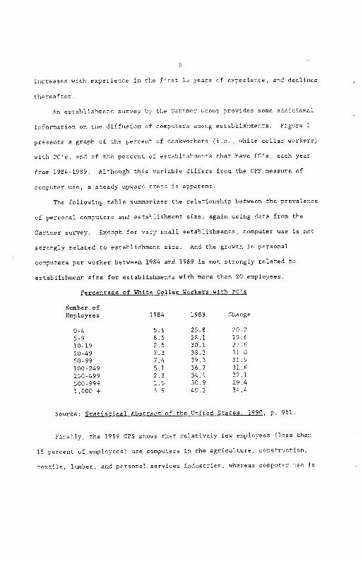
For example, in 1984 fewer then 10 percent of establishments reported that

they had personal oomputers, while this figure was over 35 peroenr in 1989

(see Figure 1) Berndt and Orilirhes (1990) estimate that the quality-

adjusted real price of new microcomputers fell by 28 percent per year

between 1982 and 1988. Several authors who have come to view technological

change as a promising explanation of changes in the wage structure have

highlighted the computer revolution as the prototypical example of such

rechno1ogcal change ,2

It is important to stress that the effect of technological change on

the relative earnings of samious categories of workers is theoretically

ambiguous. The new computerzechnology may be a cozsplemene€or e substitute

with skilled workers.3 In the former case, the computer revolution is

likely to lead to an expansion in earnings differentials based on skill,

and in the latter case it is likely to lead to compression in skill-based

differentials. This caper focuses on the narrow issue of whether employees

who use computers at wprk earn more as a result of applying their computer

skills, and whether the premium for using s computer can account for much

of the changes in the wage structure, The analysis pris4arily uses data

from Current Pcpulstion Surveys (CPS) conducted in October of 1984 and

1989. These surveys contain supplemental questions on computer use. Since

2For example, Bound end Johnson (1990) write that one explanation "attributes wage structure changes to changes in technology, brought on in

large part by the computer revolution." They conclude that this

explanation "receives a great deal of support from the data."

3sarrel. and Lichtenberg (1987) present coat function estimates for 61

manufacturing industries that suggest that skilled labor is a complement with new technclcgy. For related evidence see Welch (1970) and Oriliches

(1968)

3

CPS data spanning this time period wete widely used to document the trends

in wage diffetentials noted previously, these dsts sets ste particularly

germane. In addition to the CPS, I also examine data from the High School

and Beyond Survey (HSBS), which contains information on cognitive skills

and family background, as well as on computer use at work.

The remainder of the paper is organized as follows. Section I

presents a brief descriptive analysis of the workers who use computers at

work and details trends in computer utillzation in the U.S. in the 1950s.

Section II seeks to answer the question: Are workers who use computers at

work paid more ss a result of their computer skills? Section III sddresses

issues of possible omitted variable bias, Section IV anslyzes the impact

of computer use on other wage differentials, Finally, Section V concludes

by speculating on the likely future course of the wage structure in light

of the new evidence regarding the payoff to computer use.

To preview the main results I find that workers are rewarded more

highly if they use computers at work. Indeed, workers who use a computer

earn roughly lOlS percent higher pay than otherwise similar workers.

Although the analysis is by necessity nonexperimenral, I tentatively

conclude that a causal interpretation of the effect of computer use on

earnings may be appropriate. This conclusion is reached by fitting a

variety of models to adjust for nonrandom selection, and by controlling for

computer use off the job. I further find that because higher educated

workers are more likely to use computers at work, and because computer use

expanded tremendously throughout the lSBOa, computer use can account for a

substantial share of the increase in the rate of return to education.

4

I, Descriptive Apslysi

In spite of the wide sptead belief that computers have fundamentally

altered the wotk environment, little desctiptive information exists

concetning the chatacteristics of workers who use computers on the job.

Table 1 summarizes the probability of using a compurar at work for several

categories of workers in 1984 and 1989. The rabularions are based on

October CPS data. These surveys asked respondents whether rhey have

"direct or hands on use of computers" at work.4 Compurer use is broadly

defined, and includes programming, word processing, E-mail, computer-aided

design, etc. For one-quarter of the sample, informarion on earnings was

also collected.

Between 1984 and 1989 the percentage of workers who report using a

computer at work increased by over 50 percent, from 24.6 ro 374 percent of

rhe work force. Women, csucssisns, and highly educated workers are more

likely to use computers at work than men, African Americans, and less-

educated workers. Furthermore, rhe percentage gap in computer use between

these groups grew between 1984 snd 1989. For example, in 1984 college

gradusces were 22 points more likely to use computers sr work than high

school graduates; In 1989 this differential was 29 points.

Surprisingly, workers age 40-54 ste more likely ro use computers at

work than workers age 18-25, snd the growth in computer use between 1984

and 1989 was grestest for middle age workers. A linear probability

regression of a computer-use dummy on experience and its square, education,

and demographic variables indicates that the likelihood of using s computer

4According to rhe interviewers' instructions, "'Using a computer' refers only to the respondent's 'DIRECT' or 'HANDS ON' use of a computer with typewriter like keybosrds." The computer may be s personsl computer, minicomputer or msinfrsme computer. <See CES Field Represenrsrive's Memorsndum No. 89-20, Section II, October 1989.)

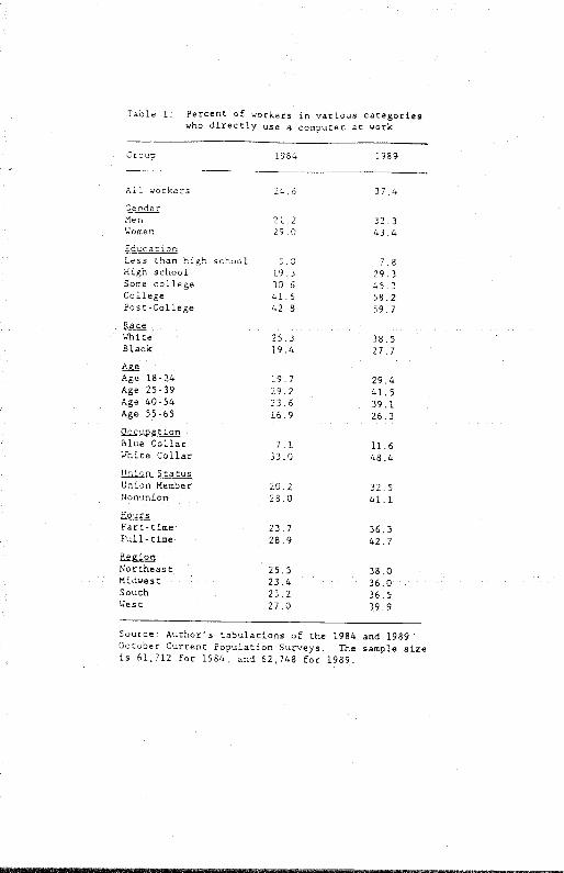
Table 1: Percent of workers in various categories who directly use a computer at work

Group 1984 1989

All workers Gender Men Women

Education Less than high school High school Some college College Post-College

Race lJh i te Black

Age 18-24 Age 25-39

Age 40-54 Age 55-65

at ion Blue Collar White Collar Union Status Union Member Nonunion

Hours Part- time Full- time

Region Northeast Midwest South West

19. 3 30.6

41.6 42.8

25.3 19.4

19. 7

29.2

23.6 16.9

7.1 33.0

20.2

28.0

25 5 23.4 23.2 27.0

7.8 29.3 45.3 58.2

59.7

38.5 27.7

29,4 41.5 39.1

26. 3

11.6 48.4

32. 5

41.1

38,0 36.0 36.5

39,9

Source: Author's tabulations of the 1984 and 1989 October Current Population Surveys. The sample size is 61,712 for 1984, and 62,748 for 1989.

24.6

21.2 29,0

37,4

32.3 43,4

23.7 36,3 28,9 42.7

increases with experience in the First 15 years of experience, and declines

thereafter

An establishment survey by the Gartner Group provides some additional

information on the diffusion of computers among establishments, Figure 1

presents a graph of the percent of deskworkers (i.e. white collar workers)

with PC's, and of the percent of establishments that have PC's, each year

from 1984-1989. Although this variable differs from the CPS measure of

computer use a steady upward trend is apparent.

The following table summarizes the relationship between the prevalence

of personal computers and establishment size, again using data from the

Gartner survey. Except for very small establishments, computer use is not

strongly related to establishment size. And the growth in personal

computers per worker between 1984 and 1989 is riot strongly related to

establishment size for establishments with more than 20 employees.

Percentage of White Collar Workers with PC'$

Number of

Employees 1984 1989 change

0-4 5.6 25.8 20.2

5-9 8.5 28.1 19.6

10-19 2.5 30.1 27.6

20-49 7.3 38.3 31.0

50-99 7.4 39.3 31.9

100-249 5.1 36.7 31.6

250-499 2.3 34.4 32.1

500-999 1.5 30.9 29.4

1,000 + 5.9 40.3 34.4

Source: Statistical Abstract of the United States, 1990, p. 951.

Finally, the 1989 CPS shows that relatively few employees (less than

15 percent of employees) use computers in the agriculture, construction,

textile, lumber, and personal services industries, whereas computer use is

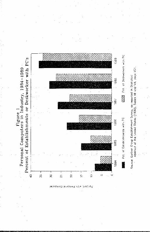
Figure 1

Personal C

omputers

in Industry,

1984—1989

Percent of

Estab1ishm

ens or

Deskw

orker w

iLh

PCs

40

35

3 30

E

25

0 C I

1984

1985

1986

1957

1988

1989

Pct.

of E

tobIihmenfs

with

PC

P

ct, of

Dekw

orkers w

Ih P

C

Source:

Gartner

Group

Establishm

ent S

urvey, as

reported in

StatistcoI

Abstract

of the

United

SLates

(1990). T

ables \1l

and V

III, poqe

951

widespread (exceeding 60 percenr of employees) in the banking, insurance,

real estate, communications, and public administration industries.

Use a nd Wa es

I have earimated a variary of staristcal models to rry to answer rhe

question: Do employees who use compurers ar work raceive a higher wage rare

as a resulr of rbeir compurer skills? I begin by summarizing some simple

ordinary least squares (OhS) estimates. The analysis is based on data from

the October 1984 and 1989 CPS, The sample consists of workers age 18-65.

(See Appendix A for further details of the sample.)

My initial approach is to augment a atandatd cross-sectional earnings

function to include a dummy variable indicating whether an individual uses

a computer at work. Let C represent a dummy variable that equals one if

the i'th individual uses a computer at work, and zero otherwise.

Observation i's wage rate, W, is assumed to depend on C, a vector of

observed characteristics X, and an error c. Adopting a log-linear

specification:

(1) lnwi_X:P+Cio+ai

where and o are parameters to be estimated. Section III considers the

effect of bias because of possible correlation between and

Table 2 reports results of fitting equation (1) by OhS, with varying

sets of covatiates (X) . In columns (1) and (4) , a computer use dummy

variable is the only right-hand-side variable. In these models the (raw)

differential in hourly pay between workers who use computers on the job and

those who do not is 31.8 percent (exp(.2765)-1) in 1984, and 38.4 percent

Table 2: OLS regression escirrates of the effect of computer use on pay Dependent variable: in (hourly wage)

Independent Variable

Qçgbgr 1989 (1) (2) (3) () (5) (6)

1rtercept 1 937 (0.045)

0,750 (0,023)

0.928 (0.026)

2.086 (0.006)

0 905 (0.024)

1 054 (0426)

Uses computer at work (1—yes)

0.276 (0.010)

0.170 (0.008)

0 140 (0.008)

0.325 (0.009)

0.185 (0.008)

0.162

(0.008)

Years of aducarion

--- 0.069 0.0U1,

0.048 (0.002)

--- 0.075 (0.002)

0.055

(0.002)

Experience --- 0.027 (0,001)

0.025 (0.001)

--- 0.027

(0001) 0025

(0.001)

Experience-Squared 100

- - - -0.041 (0.002)

-0.040

(0.002)

-- - -0.041 (0.002)

-0.040

(0.002)

Black (1—yes) --- -0.095 (0.013)

-0 066 (0.012)

--- -0.121,

. (0.013) -0.092

(0.012)

Other race (i—yes)

--- -0.105 (0.020)

-0.079 (0.019)

--- -0.029 (0.020)

-0,015

(0.020)

Part-time (1—yes)

--- -0 256 (0.010)

-0.216 (0,010)

--- -0.221 (0.010)

-0,183 (0.010)

Lives in SMSA

(1—yes)

--- 0.111 (0.007)

0.105 (0.007)

--- 0.135 (0.007)

0.130 (0,007)

Veteran (1—yes)

- -- 0.038 (0,011)

0,041 (0.011)

--- 0,025 (0.012)

0.031 (0.011)

Female

(1—yes)

--- -0.162

(0.012) -0.135 (0,012)

--- -0.172 (0.012)

-0.151

(0.012)

Harried (1—yes)

--- 0.156 (0.011)

0.129 (0.011)

--- 0.159 ,

(0.011) 0.143 (0.011)

Married*Female --- -0.168 (0015)

-0,151 (0.015)

--- -0.141 (0,015)

-0.131

(0.015)

Union member (1—yes)

--- 0.181 (0.009)

0.194 (0.009)

--- 0.182 (0.010)

0.189 (0.010)

S Occupation Dums. No No Yes No No Yes

R2 0051 0.446 0.491 0.082 0.451 0.486

Notes: Standard errors are shown in parentheses. Sample size is 13,335 for 1984 and 13379 for 1989. Columns 2,3,5,and 6 also include 3 region dummy variables,

(exp(.325)-i) in 1989. In columns (2) and (5) several covariates are added

to the regression equation, including educatico,, potential experience and

its square, gander, and union status. Including these variables reduces

the computer premium to 18.5 percent in 1984 and to 20.6 percent in 1989.

Even after including these covariates, however, the computer dummy variable

continues to have a aicable and statistically significant effect on wages,

with t-rarios of 21.3 in 1984 and 23.1 in 1989.

It is nor ricer whether occupation dummies are appropriate variables

to include in these wage regressions because computer skills may enable

workers to qualify for jobs in higher paying occupations end industries.

For example, one would probably not want to control for whether a worker is

in the computer programming occupation while estimating the effect of

computer use on earnings. Nevertheless, columns (3) and (6) include a set

of 8 one-digit occupation dummies. These models still show a sizable pay

differential for using a computer at work. In 1989, for example, employees

who use computers on the job earn 17.6 percent higher pay than employees

who do nor use computers on the job, holding education, occupation, and

other cherecterstics constant. If 44 two-digit occupmtion dummies are

included in the model in column (6) instead of one-digit occupation

dummies, the computer use wage differential is 13.9 percent, with e t-rario

of 15.5.

a. Employer characteristics

Although I em mainly concerned about bias because of omitted employee

characteristics that etc correlated with computer use at work, it is

possible that characteristics of employers are correlated with the

provision of computers and the generosity of compensation. Such a

relationship might exist in a rent-sharing model in which employees are

able to capture some of the retutn to the employer's capital stock.

Unfortunately there is only a limited amount of informatiun about employer

characteristics in the CFS. However, if 48 two-digit industry dummies are

included in a model that includes two-digit occupation dummies and the

covatiates in column (6), the compoter use wage diffetential is 11.4

percent, with a t-ratio of l3.O.

Information on employer size is not available in the October CPS, but

two findings soggest that the computer differential is not merely

reflecting the effect of (omitted) employer size. First, establishment-

level surveys do not show a strong relationship between computer use and

establishment size (e.g., Hitschorn, 1991). Second, in a recent paper

Reilly (1990) uses a sample of 607 employees who worked in 60

establishments in Canada in 1979 to investigate the relationship between

establishment size and wages. Reilly estimates wage regressions including

a dwmsy variable indicating access to a computer. Without controlling for

establishment size, ha finds that employees who have access to a computer

earn 15.5 percent (t—S.7) higher pay. When he includes the log of

establishment size the computer-wage differential is 13.4 percent (t—3.9).

Finally, I have estimated the model in column (5) separately for union

and nonunion workers. The premium for computer use is 20.4 percent

(t-rario—23) in the nonunion sector, and just 7.8 percent (t—4.3) in the

union sector. Since unions have been found to compress skill differentials

(see Lewis, 1986 and Card, 1991), this finding should not be surprising.

5Results for 1984 are similar: the wage differential falls to 11.3 percent if 44 occupation dummies are included, and to 9.0 percent if 48

two-digit industry dummies are included.

However, if one believed that the premium for work-related Computer use is

a result of employees oapturing firms' oaptal rents rather than a return

to a skill, it is diifioult to explain why the premium is so muoh larger in

the nonunion seotor than in the union seotor.

Time

The results in Table 2 indioate that, if anything, the estimated

reward for using a oomputer at work inoreased slightly between 1984 and

1989. got example, based on the models in oolumns (3) and (6), between

1984 and 1989 the oomputer (log) wage premium inoreased by .022. The

standard error of this estimate is .011, so the inorease is on the margin

of statistioal signifioanoe. There is oertainiy no evidenoe of a deoline

in the payoff for oomputer skills in this period,

This finding is of interest for two reasons. First, given the

substantial expansion in the supply of workers who have coaputer skills

between 1984 and 1989 one might have expeoted a deoline in the wage

differential assooiated with Computer use at work, oeteris paribus. The

failure of the wage differeotial for oomputer use to deoline suggests that

the demand for workers with oomputer skills may have shifted out as fast

as, or faster than, the outward shift in the supply of oomputer-literate

workers. This hypothesis is plausible givem the remarkable deoline in the

prioe of Computers and the expansion in uses of oomputers in the 1980s.

A seoond reason why the slight inorease in the wage differential

assoofated with oomputer use is of interest oonoerns the effeot of possible

nonrandom seleotion of the workers who use Computers. Companies are likely

to provide Computer training and equipment first to the workers whose

produotivity is expeoted to inorease the most from using a Computer. This

10

would pose a problem for the interpretation of the Ohs estimates if these

workers would have earned higher wages in the absence of computer use, The

large increase in the number of workers who used coeputers at work between

1984 and 1989 was iiaely to have reduced the average quality of workers who

work with computers, wnich would be expected to drive down the average wage

differential associated with computer use. However, the slight increase in

the computer wage premium between 1984 and 1989 suggests that nonrandom

selection of the workers who use computers is not the dominant factor

behind the positive association between computer use and wages.

The other variables in Table 2 generally have their typical effects on

wages, and their coefficients are relatively stable between 1984 and 1989.

One notable exception is the rate of return to education, which increased

by ,g percentage points between 1984 and 1989, even after holding computer

use constant. And the black-white wage gap increased while the wage gap

between whites and other races declined in these years.

c. Sperifir compurer tasks

The 1989 CPS asked workers what tasks they use their computer for.

Individuals were allowed to indicate multiple tasks. I have estimated the

model in column 6 of Table 2 including a set of computer-task dummy

variables. (These estimates are available on request.) Interestingly,

rhese results show that me most highly rewarded task computers are used

for is electronic mail, probably reflecting the fact that high-ranking

executives often use E-mail, On the other hand, these results show no

premium for lndivdoals who use a computer for playing computer games. And

book keeping, desk top publishing, and inventory control have slightly

lower rewards than the average task.

III. Is the Computer Wage Differential Real or Illusory?

A critical concern in interpreting the OLI regressions reported above

is that workers who use computers on the job may be more able workers, and

therefore may have earned higher wages even in the absence of computer

technology. Further, the finding that the computer-wage differential is

attenuated when covariates are included in the OLS regressions suggests

that important variables may be omitted that are positively correlated with

both computer use and earnings. I have tried four empirical strategies to

probe whether the computer-pay differential is a real consequence of

coaputer use or is spurious.

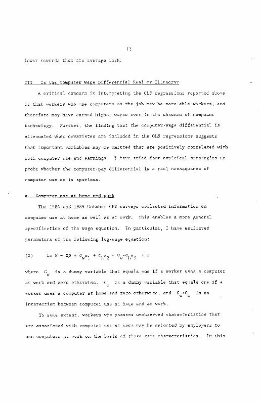
a. Computer use at home and work

The 1984 and 1989 October CPS surveys collected information on

computer use at home as well as at work. This enables a more general

specification of the wage equation. In particular, I have estimated

parameters of the following log-wage equation:

(2) ln W — xfi + Cwel + Chn2

+ CCha3 + C

where tw is a dummy variable that equals one if a worker uses a computer

at work and zero otherwise, Ch is a dummy variable that equals one if a

worker uses a computer at home and zero otherwise, and C 'C is an wh interaction between computer use at home and at work.

To some extent, workers who possess unobserved characteristics that

are associated with computer use at home may be selected by employers to

use computers at work on the baste of those same characteristics. In this

12

case controlling for whether workers use a computer at home would capture

at least some of the unobserved variance in the error term that is

cortelared with tunpurer ,se at work. If the positive association between

computer use at wotk and nay is spuriously reflecting correlation between

computet use and omitted variables we would expect 01 02 and 01 —

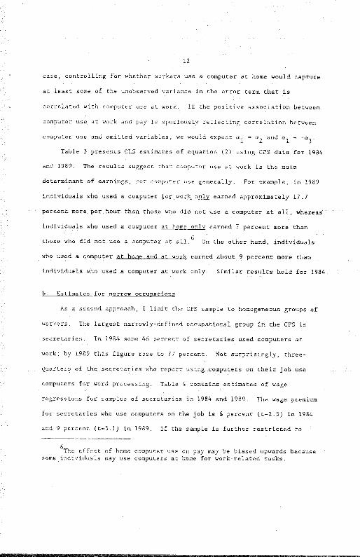
Table 3 presents OIS estimates of equation (2) using CFS data for 1984

and 1989. The results suggest that computer use at work is the main

determinant of earnings, not computer use generally. For example, in 1989

individuals who used a computer wqxkonl' earned approximately 17.7

percent mote pet hour than those who did not use a computer at all, whereas

individuals who used a computer at hnsie only earned 7 percent mote than

those who did not ume a computer at alL6 On the other hand, individuals

who used a computer at home and at work earned about 9 percent mote than

individuals who used a computer at work only. Similar results hold for 1984.

isa res f or na mmcv cc cc a t ion s

As a second approach, I limit the OPS sample to homogeneous groups of

workers, The largest narrowly-defined occupational group in the CPS is secretaries - In 1984 some 46 percent of secretaries used computers at

work; by 1989 this figure rose to 77 percent. Not surprisingly, three-

quartets of the secretaries who report using computers on their job use

computers for word processing. Table 4 contains estimates of wage

regressions for samples of secretaries in 1984 and 1989. The wage premium

for secreraries who use computers on the job is 6 percent (r—2,5) in 1984

and 9 percenr (t—3.l) in 1989, If the sample is further restricted to

6The effect of home computer use on pay may be biased upwards because some individuals say use computers at home for work-related tasks,

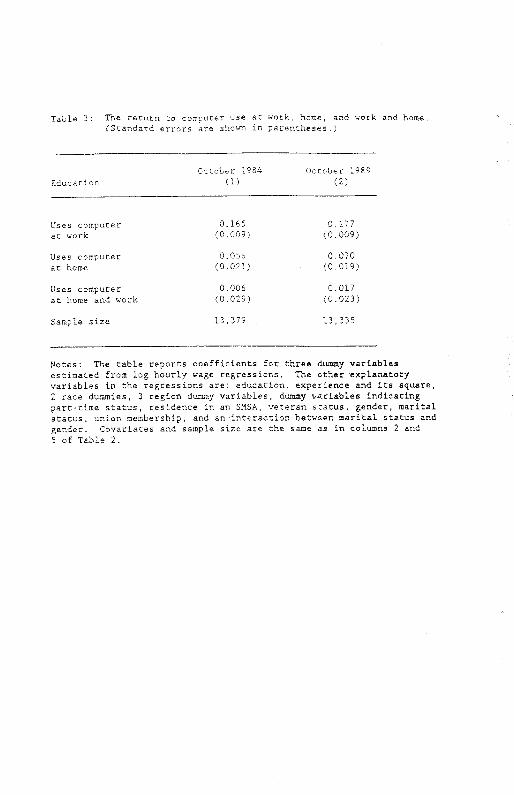
Table 3: The return to computer use at work home, and work and home. <Standard errors are shoi in parentheses.)

Education October 1984

(1) October 1989

(2)

Uses computer at work

0.165 (0.009)

0.177 (0.009)

Uses computer at home

0.056 (0.021)

0.070 (0.019)

Uses computer at home and work

0.006 (0.029)

0.017 (0.023)

Sample size 13379 13335

t1otes: The table reports coefficients for three dummy variables estimated from log hourly wage regressions. The other explanatory variables in the regressions are: education, experience and its square, 2 race dummies, 3 region dummy variables, dummy va.riables indicating part-time status, residence in an SMSA, veteran sOatus, gender, marital status, union membership, and an interaction between marital status and

gender. Covariares and sample size are the same as in columns 2 and

5 of Table 2.

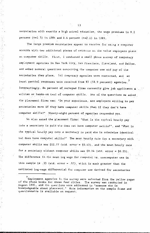
13

secretaries with exactly a high school education, the wage premiums is 9.2

percent (t—33) in 1984 and 8.6 percent (t—21) in 1989.

The large premium secretaries appear to receive for using a computer

accords with two additional pieces of evidence on the value employers place

on computer skills. First, I conducted a small phone survey of temporary

employment agencies in New York City San Francisco, Cleveland, and Dallas,

and asked several questions concerning the computer use and pay of the

secretaries they place. 141 temporary agencies were contacted, and at

least partial responses were received from 83 (58.9 percent) agencies.7

Interestingly, 84 percent of surveyed firms currently give job applicants a

written or hands-on test of computer skills. One of the questions we asked

the placement firms was: "In your experience, are employers willing to pay

secretaries more if they have computer skills than if they don't have

computer skills?" Ninety-eight percent of agencies responded yes.

We also asked the placement firms: "What is the typical hourly pay

rate a secretary is paid who does not have computer skills?", and "What is

the typical hourly pay rate a secretary is paid who is otherwise identical

but does have computer skills?" The mean hourly rate for a secretary with

computer skills was $12.77 (std. error —$0.43), and the mean hourly rate

for a secretary without computer skills was $9.14 (std. error — $0.25). The difference in the mean log wage for computer vs. noncomputer use in

this sample is .33 (std. error — 02), which is much greater than the

estimated log-wage differential for computer use derIved for secretaries

7Employment agencies in the survey were selected from the yellow pages of the phone books for these four cities. The survey was conducted in August 1991, and the questions were addressed to "someone who is knowledgeable about placement." More information on the sample frame and questionnaire is available on request.

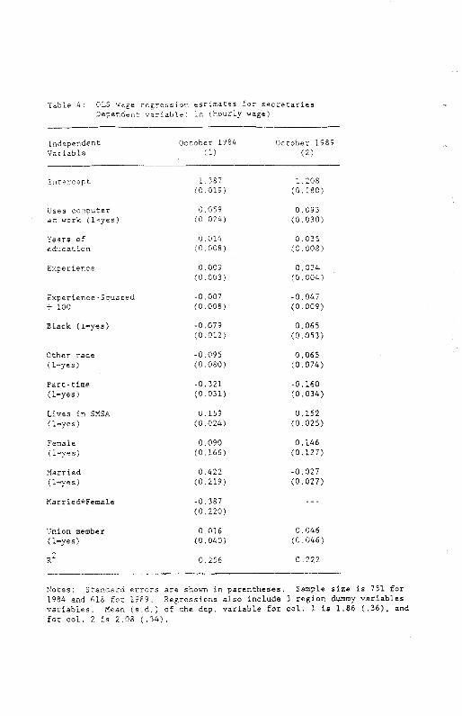
Table 4: OLS wage regression estimates for secretarLes Dependent variable: in (hourly wage)

Independent October 1984 October 1989 Varab1e (1) (2)

Intercett 1387 1208 (0019) (0.180)

Uses computer 0.059 0.093 at work (1-yes) (0.024) (0.030)

Years of 0.014 0.035 education (0.008) (0.008)

Experience 0.009 0.024 (0.003) (0.004)

Experience-Squared -0.007 -0.047 4 100 (0.008> (0.009)

Black (1—yes) -0.079 0.065 (0.012) (0.053)

Other race -0.095 0.065

(i—yes) (0.080) (0.074)

Part-time -0.321 -0.160

(1—yes) (0.031) (0.034)

Lives in SMSA 0.159 0.152

(1—yes) (0.024) (0.025)

Female 0.090 0.146

(1...yes) (0.166) (0.127)

Married 0.422 -0.027

(1—yes) (0.219) (0.027)

Marrfed*Fese1e -0.387 (0,220)

UnSon member 0.016 0.046

(1—yes) (0.040) (0.046)

0.256 0.222

Notes: Standard errors are shown in parentheses. Sample size is 751 for 1984 and 618 for 1989, Regressions aiso include 3 region dummy variables variables, Mean (s.d.) of the dep. variable for col. 1 is 1.86 (.36), and

for col, 2 is 2,08 (.34).

14

using CPS data,

Lastly, we asked the employment agencies whether they provide computer

training to the workers they place, and who pays for the training Some 62

percent of employment agencies responded that they provide up-front

training for the workers they place. And in 96 percent of the instances in

which training is provided the employment agency pays for the training.

In the remaining 4 percent the employee pays for training; none of the

firms responded that the firm where the worker is placed pays for training.

The finding that employment agencies pay for computer training for

temporary employees is quite surprising because the training is likely to

be of general use. Moreover, this phenomenon differs from on-the-job

training since temporary workers cannot pay for training by taking a lower

initial wage because they receive the training before they start work, and

they are under no obligation to subsequently work. The fact that temporary

agencies seem to find it profitable to provide computer training to the

workers they place suggests there is a substantial return to computer skills.

Second, a survey of 507 secretaries employed by large firms conducted

by Kelly Services (1984, p. 13) provides some additional evidence on

whether employers truly pay a wage premium to secretaties with computer

skills. This survey found that 30 percent of secretaries received a pay

raise as a result of obtaining word processing skills.

Although the estimated wage premium for secretaries who use computers

at work based on CPS data may appear to be large by economic standards

(e.g., at least as important as one year of additional schooling), it does

not seem implausible given this external evidence. In fact, the phone

survey of temporary employment agencies suggests that the CI'S may

underestimate the premium for computer use. From a practical perspective,

the large wage differential for secretaries who are ptoficent at operating

computers suggests that public-sector training programs might profitably

concentrate on providing trainees with computer skills.

I have estimated the computer wage differential for six additional

8 white collar occupations. To summarize these results the estimated

computer differential (a) and standard error for these occupations in 1989

are: .137 (.035) for managers; .101 (.044) for registered nurses; .060

(.038) for school teachers; .185 (.046) for sales supervisors; - .052 (.073)

for sales representatives; and .089 (.062) for book keepers. Further

analysis indicates that the computer premium mends to be smaller in thtee-

digit occupations that have a greater proportion of wctkers using

computers.

c. Remested cross-section methods

Thus far, we have treated the 085 data sets as independent cross-

sections. We can also take advantage of the repeated nature of the 085

data sets by linking cohorts over time. Specifically, write the wage

equations for 1984 (indicated by subscript I) and for 1989 (indicated by

subscript 2) as:

(3) in W.1 + CilOl

+ cii

(4) In W,. — + 0il°2

+

8The occupations were selected on the basis of sample size: three-

digit occupations wfth 180 or more observations were selected. (Elementary school, secondary school, and special education teachers were combined.) The regressions included the same variables as in column (5) of Table 2.

See Appendix A for further details.

16

If we are willing to assume that a — a2 — a is constant between 1984

and 1989, we can estimate the computer-use wage differential using repeated

cross-section/multiple cohort models.9 This estimator takes advantage of

the fact that the proliferation in computer use was not constant across

cohorts. Because the same set of indivLduals are in these cohorts over

time (ruling out labor force participation issues) computer use is not

correlated with unobservables at the cohort level, In principle, this

approach yields a consistent estimate of a even if C, and c8, are correlated.

Specifically, define (j—l929 1959) as a set of cohort dummy

variables that equal one if an individual is born in year j and zero

otherwise, and define Ti as a period dummy variable that equals one if an

individual is observed i0 1989 and zero if observed in 1984, Under the

assumptions listed above, we can estimate the following equation for a

pooled sample of individuals drawn from the 1984 and 1989 October CPS's:

(5) in U. X8,fl1

+ T8,.X8,(82 + T.8 + + C.a + c1.

Equation (5) is estimated by two-stage least squares (TSLS), using T8,Y.

as

exclusion restrictions

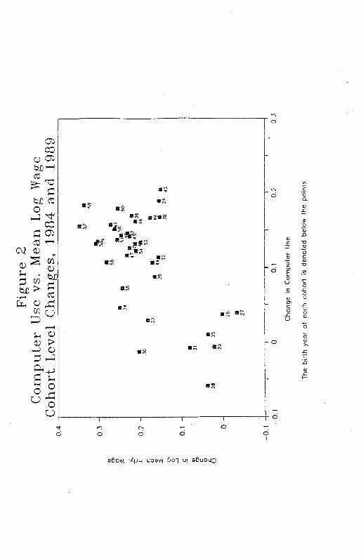
Figure 2 illustrates the relationship between the change in mean log

hourly earnings for a birth cohort and the change in the proportion of

workers in that cohort using a computer at work over the period 1984-89.

Each point represents the experience of a single year-of-birth cohort

ranging from 1924 to 1959, and the birth year is indicated on the graph,

9See Deaton (1985) and Beckman and Robb (1985) for references on repeated cross-section methods.

10 It is implicitly assumed that var(o8,1)

— var(e8,2).

Figu

re 2

Com

put.e

r U

sevs

.M

ean

Log

Wag

eC

ohor

t Lev

el C

hang

es, 1

984

and

1989

0.4

-

N 5?N 58

03-

N0)

55N

o54

lN

NN

Sso

I0.

2-N

54N

4630

CN

52o

N N

N4,

39N

N N

3238

240) 0 -j

0.1-

N 310' C 0 £

NN

o28

N 2

529

0N 26 N 2?

—0.

1

—0.

10

0.1

0.2

03

Cha

nge

in C

ompu

ter

Use

The

birt

h ye

ar o

f eac

h co

hort

is d

enot

ed b

elow

the

poin

ts.

17

Sume birth cohorts clesrly experieoced greater expansion in computer ose

than others, Further, the scatter diagram displays an opward sloping

relarionshtp between earnings growth and the growth in computer use for

these birth cohorts. However, the upward sloping relationship exhibited in

the figure is largely a result of slower wage growth icr older workers,

Equation (5) Includes a set of unrestricted cohort dummies and a year dummy

to control for differences in age.

Table 5 reports estimates of equation (5). The sample has been

narrowed to individuals born between 1929 and 1959 to avoid major

life-cycle changes in labor force participation. The model in column (1)

simply reports the Ohs estimate of equation 5. Columns (2) and (3)

identify the computer differential from cohort variation in the growth in

oompurer use between 1984 and 1989. Notice that the models differ insofar

as which of the X-vmriables are free to have varying coefficients over

time, The model in column (2) is the least restrictive specification: all

of the X-variables are allowed to have time-varying coefficients, but the

cohort dummies and computer dummy are restrIcted to have constant effects

over time. Column (3) only frees up the gender, race, and education

variables over time,

The TSLS models in columns (2) and (3), which rely on the repeated

cross-sections for identification, show that the wage differential for

using a computer on the job is about 29 percent, about twice as large as

their standard errors. Although the TSLS estimate is larger than the OhS

estimate, the difference between them is not statistically significant.

However, both 2SLS models fail a test of error-instrument orthogonality at

conventional levels of significance. Futhermore, the estimates are

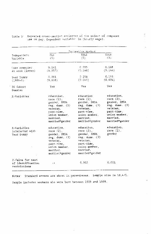
Table 5: Repeated cross-section estimateS of the effect of computer use on pay. Dependent variable: In (hourly wage).

Independent

Estimation Method OLS TSLS TSLS

Variable (1) (2) (3)

Uses computer 0181 0285 0.288

at work (1yes) (0.007) (0.148) (0.144)

Year Dummy 0.201 0.208 0.115

(l9891) (0.038) (0.040) <0.034)

30 Cohort Yes Yes Yes Dummie a

X-Variabies education race (2), gender, SMSA

reg. dums. (3)

veteran, part-time, union member, married, married*gender

education, race (2), gender, S8SA reg. dums. (3) veteran, part-time, union member, married, married*gender

education, race (2), gender, SMSA

reg. dums. (3) Veteran, part-time, union member, married, married*gender

X-Variables education, education, education, Interacted with race (2), race (2), race (2), Year Dummy gender, SMSA

reg. dums. (3) veteran, part-time, union member, married, married*gender

gender, SMSA

reg. dums. (3) veteran, part-time, union member, married, matried*gender

gender

P-Value for test of identification - 0.002 0.001 restrictions

Notes: Standard errors are shown In parentheses. Sample size is l8,471.

Sample includes workers who were born between 1929 and 1959.

18

extremely sensitive to minor changes in the specification. For example if

experience and experience-squared are included instead of the 30 cohort

duacies, the computer (log) wage differential increases to 045 (t—48).

d. Estimates based on the Rich Srhool and Beyond Survey

To control for a more comprehensive sot of personol characteristics, I

have examined data from the High School and Beyond Survey. This

longitudinal data act contains information on comparer use, achievement

test scores, and school performance for individuals who were high school

sophomores or seniors in 1980. The 1984 wave of the survey asked about

earnings and work experience. I restrict the sample to workers with

exactly a high school education because anyone with additional schooling

would riot have spent much time in the labor market by 1984. Further

description of the sample and variables is provided in Appendix B.

Unfortunately, the computer use question in the HSBS is not ideally

suited for my purposes. Information on computer use at work was collected

only in the 1984 wave of the survey. In that year, individuals were asked

whether they ever used a computer on a job. Some individuala may have used

a computer on an earlier job but not on their present job. Consequently,

computer use and earnings are not perfectly aligned. Nevertheleaa, the

USES provides another data aet with which to examine the robuatneaa of the

effect of computer utilization at work on earnings.

Table 6 presents several OLS estimates of the effect of computer use

at work on wages using the USgS. The first column simply reports the

difference in the mean log wage rate in 1984 for workers who have used a

computer at work and those who have not. The differential of 11 log

points is lower than the estioare derived from the October 1984 CFS.

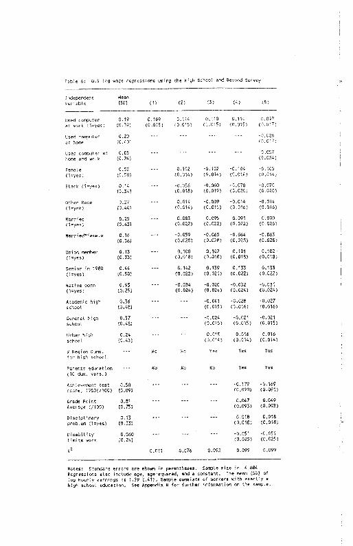
table 6: 040 log wage regresaisna swing the high Scnool wed Beyond Survey

Used cavrpcter 0.20

so hone 10.40]

Used cstputer at 4.05 hrvoe orb work [0.24]

Fenele 0.52

<iyas] [0.50]

Blank Kiyea) 014 [0,34]

Other Pace 0,27

41yes] [3.44]

Married 0.25

4175001 [3.42]

Merried*Peesale 0.16 [0,36]

Oaf at ewither 0,13

([eyes) 00.33]

Senior in 1930 0.44

417500] 10,50]

Native born 0.93

ll=yesl [3.25]

bcedeteic high 0.36

school [0.40]

General high 0.37 school [0.40]

Urban high 0,24 school [0.43]

O Region 0u00. br high school

Parents education [10 thee. oars,]

Achieceesent test 0.00 score, 10001/100] [0.09]

grade Hoist 0,51 boerege 4/100] 10.75]

Oiaciplieary 0.13 grsble'a ll75esl [0.33]

Oisabi]ity 0,060 lieita asrk [0.24]

I rdepaeden] Variable

Mean [00] 51] 42] [30 14] 151

Used coocscter 0.19 0.109 0.114 0.110 0,110 0.007 us cork 1175e51 [0,39] 10.015] 10.015] 10.015] lO,0151 40.017]

'0.026

40, 0] 71

0.057

-0.152 '0.102 '0.134 '4.105

10.0141 40,014] 10.0141 14,014]

'0.056 '0,060 '0.070 '0,070 10.0131 10,019] 10.020] 10.020]

0.014 '0.009 '0.014 '0.014 40.014] 10.0151 40,5104 40.016]

0.003 0.095 5.091 0.003

10.0021 40.0)2] 40.522) 43.026]

'0.059 '0.065 '0,064 '0.063 10.020] 10.028] 10.0231 10,0231

0.100 0.102 0.101 0.100

10.0181 40,013] [0.013] 40,018]

0,142 0,139 0,133 0.133

10.022] 10.021] 15.022] 10.020]

'0,034 '0.020 '0,032 '0.031 (0.024] (5.024] 10.024] (0,0241

'0.041 '0.023 '0.007 (0.015) (0.016] (0.0161

'0.024 -0.021 '0.021

(0.0151 40,015] 40.0151

0.010 0.016 0.016 (0,014] <0.014] 40,014]

ifs ho Yes Yes Yes

Na Mo Bc Yea tea

'0,175 '0.169 (0,090) 43.091]

0,047 0.049

45.0931 (0.0931

0.018 0,018 (0.018] 40,016]

'0,051 '0,351

10.025] (0,0251

0.011 0.076 0.092 0.099 0.099

Hates: Ytardard errsra are shown in parentheses. SastRale sloe is 4,684,

Regressions alac inc]boe fle, ige'aiared, at4 ceesatant, the aasan [WI of lag hcsr]y eereir.gs a 1.59 [.41], Saseple consists of avrkers with eoactly high school education, See bppeeabie H far further feforeatian an the saep]e.

19

Column (2) adds several demographic variables, column (3) adds several

variables measuring the kind of high school the individual attended, and

column (4) adds the worker's self-reported high schuol grado puirit average,

a composite test score measuring reading and mathematics skills, aid

additional background characteristics (eg , parents' education),

Including these variables has little effect on the magnitude of the wage

premium for work-related computer use.

Interestingly, in the HSBS data there is a statistically significant,

positive association between a worker's propensity to use a computer at

work and both his achievement test score and grade point averege. For

example, a one standard deviation increase in the cognitive test measure is

associated with a 2.7 percentage point increase in the likelihood of

computer use at work,11 A possible concern about the estimates in colwn

(4) is that the test score variable has a negative effect on earnings, Tu

explore this further, in other estimates I have used workers' 1982

achievement test score, which is available otly for sophomores, as an

instrumental variable for their 1980 test score. However, these estimates

continue to show a negative relationship between achievement test scores

and wages,

The 1984 wave of the HSBS also inquired about individuals'

"recreational" use of computers; that is, whether they have used a cuo.putcr

outside of work and school. I have used this infurmation to est,,mace

equation (2) for the Hill sample, where "home" computer use denotes

11The association between "recreational" computer use (i.e , computer use that is unrelated to work or school) and test scores is even higb'c'. For example, a one standard deviation increase in the test score taises probability of recreational computer uae by 9.6 percentage points.

20

"recreational' use, These results are reported in column (5). Similar to

the estimates from the OPS, the results indicate that computer use at work

is an important determinant of earnings, whereas computer use at home does

not aignficantly affect earnings.

IV. The Effect of the Commuter Revolution o Other Wage Dijjp,isls The previous sections tentatively establish that workers who use

computers on their jobs earn more as a result of their computer skills. A

natural question to raise is: thfl.sffecthas the proliferatio,,st

c2p2Mters..Eatk1.Qn...the relatjpnship between earnings and ojg.

variables, auth as education? This issue is particularly relevant because

computer use, and the expansion of computer use, has not been uniform

across groups. Here I only estimate the direct effect of holding computer

use constant on other earnings differentials; potentially important spill

over effects of computer use on non-computer users (e.g., the effect of a

secretary using a computer on his or her boss) are not taken into account.

To explore the effect of computer use on other wage differentials,

Table 7 presents OLS estimates of wage equations in 1984 and 1989, with and

without including the computer use dummy variable. Columns (2) and (5)

simply reproduce estimates in Table 2. Columns (3) and (6) teport an

alterative specification, which includes both a computer dummy and an

interaction between the computer dummy and years of education. This

specification indicates that the computer differential is greater for more

highly educated workers.

Notably, the table shows that the rate of return to education

increased by one point between 1984 and 1969 if the computer dummy is not

Table 7: OLS regression estimates of the effect of computer use on pay Dependent variable In (hourly wage)

Independent October 1984 October 1989 Variable (1) (2) (3) (4) (5) (8)

Uses computer -- 0170 0073 -- 0.188 0.005

at work (1—yes) 0.008) (0.048) (0.008) (0043)

Computer Dum, -- .. 0.007 -- -- 0.013

x Education (0.003) (0003)

Years of 0.076 0 069 0.067 0.086 0.075 0.071 education (0001) (0.001) (0.002) (0.001) (0.001) (0002)

Experience 0.027 0.027 0.027 0.027 0.027 0,027 (0.001) (0.001) (0.001) (0.001) (0.001) (0.001)

Exper, Squared -0.042 -0.041 -0.042 -0.044 -0.041 -0.042 100 (0.002) (0.002) (0.002) (0.002) (0.002) (0.002)

Elack (1—yes) -0.106 -0.098 -0.099 -0.141 -0.121 -0.122 (0.013) (0.013) (0.013) (0.013) (0.013) (0.013)

Other race -0.120 -0.105 -0.106 -0.037 -0.029 -0.032 (1—yes) (0.020) (0.020) (0.020) (0.021) (0.020) (0.020)

Part-time -0.287 -0.256 -0.256 -0.261 -0.221 -0 221

(1—yes) (0.010) (0.010) (0.010) (0.010) (0.010) (0.010)

Lives in SMSA 0.123 0.111 0.111 0.148 0.138 0,138

(1—yes) (0.007) (0.007) (0,007) (0.007) (0.007) (0.007)

Veteran 0.043 0.038 0.039 0.027 0.025 0,029

(1—yes) (0.011) (0.011) (0.011) (0.012) (0.012) (0.012)

Female -0.140 -0.162 -0.160 -0.142 -0.172 -0.168

(1—yes) (0.012) (0.012) (0.012) (0.012) (0.012) (0.012)

Married 0.162 0.156 0.156 0.169 0.159 0.158

(1—yes) (0.011) (0,011) (0.011) (0.011) (0.011) (0.011)

Married*Female -0.171 -0.168 -0.168 -0.146 -0.141 -0.139

(0.015) (0.015) (0,015> (0.015) (0,015) (0.015)

Union member 0.167 0.181 0.181 0,164 0.182 0.182

(1—yes) (0.009) (0.009) (0.009) (0,010) (0.010) (0.010)

R2 0.429 0,446 0.446 0,428 0,451 0.452

Mean-Sq. Error 0.168 0.163 0.163 0.176 0,169 0.169

Notes: Standard errors are shown in parentheses. Sample size is 13,335 for

1984 and 13,379 for 1989. Regressions also includes 3 region duzy varIables and an intercept.

21

included in the regressions; if the computer dummy iS included the return

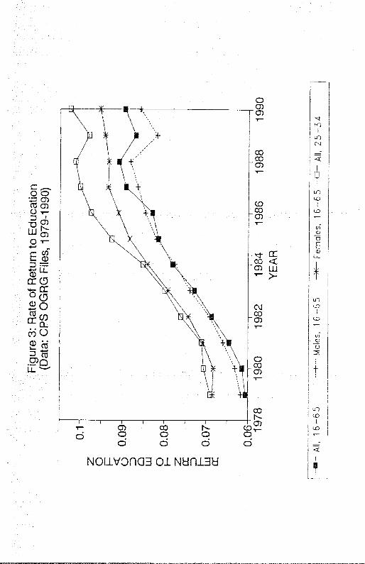
to sducstion increased by 0.6 points. To further investigate the time-

series trend in the return to education, Figure 3 plots estimates of the

return to education for the full sample and for three subsamples, based on

dets from the Outgoing Rotation Group (OGRG) Files of the CPS each ymet

from 1979l99O.l2 The figure indicates that the log-linear estimate of the

return to education increased steadily between 1979-1988, although the

upward tend appears to have levelled off in 1989-90.

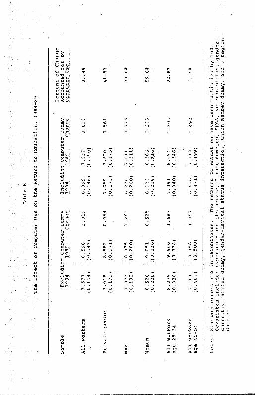
I have examined the effect of computer use on the retutn to education

In several other samples. These results ate summarized in Tables 6 and 9.

First consider Table 8, which reports estimates of the rate of return to

education (times 100), with and without including a dummy indicating

computer use at work. The first subsample is private sector wockets)3

8etween October 1984 and 1989 the conventional 01.5 estimate of the return

to education in the private sector incteesed by .96 points. If, however,

computer use is held constant, the return to education is estimated to have

increased by .56 points. Thus, it appears that increased computer use can

"account" for 41.6 percent (— 100•(.96-.56)/.96) of the increase in the

return to education in the private sector.

Turning to the other samples, the return to education increased by

less fot women than for men between 1984 and 1989. Holding computer use

constant accounts fot over half the increase in the return to education

12The sample and covariates were defined to be similar to the samples used in column (1) of Table 7. Further details are available on request.

13Katz ond Krueger (1991) find that the increase in the return to education was much greater for private sector workers than for public sector workers.

z 0 H

0 a uJ 0 I—

z cc

EL

cc

Fem

ales, 1

6 —

65 '

All,

25—34

Figure

3: R

ate of

Return

to E

ducation (D

ata: C

PS

O

GR

G

Files,

1 979-1

990)

0.1

0.0

0.08

0.07

0. 1978

1980 1982

1984 1986

1988 Y

EA

R

I A

ll, 1

6-65 M

ales, 1

6 -65

22

observed fat female workers, and nearly 40 percent for male workers. Also?

it appears that although the return to education increased by more for

younger wotkets than for older workers, controlling for computer use

accounts for a larger share of the increase for older workers.

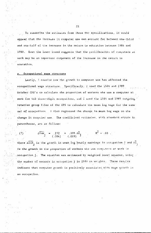
Table 9 reports results with and without including both a computer use

dummy and an interaction between computer use and years of education.

Specifically, I estimate the equation:

(6) In W Xifi + Ep ÷ P.o + C.E.1 + c.

where In W. represents the log hourly wage rate, education, C. a

computer use dummy variable, and a set of covariates. I am interested

in the question: What would the return to education be if computer use

remained constant at its 1984 level? This is given by p + q..266 , where

.246 is the proportion of workers that used computers in 1984.

Because -y > 0 for most subsamples and has increased over time (compare

columns (3) and (6) of Table 7), the specification that includes the

interaction between the computer use dummy and education tends to account

for a somewhat greater share of the increase in the return to education.

Fur example, the augmented specification accounts for 50.5 percent of the

increase in the return to education for the entire sample, and neatly two-

thirds of the inctease for private sector workers. For women, increases in

computer use appear to account for more than the total obsecved increase in

the return to education. For older workers, however, the wage differential

for using a computer declines with education (y < 0) , so more of the

increase in the return to education for this sample is accounted for by

computer use in the duassy variable specification in Table 8.

Table

8

The

Effect

of

Computer

Use

on

the

Return

to

Education,

1984-89

Percent

of

Change

Sample

Excluding

Computer

Dummy

Including

Computer

Dummy

Accounted

for

by

19Q..i

M

Change

1989

Computer

Use

All

workers

7.577

8.596

1.019

6.899

7.537

0.638

37.4%

(0.144)

(0.147)

(0.146)

(0.150)

Private

sector

7.918

8.882

0.964

7.059

7.620

0.561

41.8%

(0.172)

(0.171)

(0.173)

(0.175)

Men

7.073

8.335

1.262

6.236

7.011

0.775

38.6%

(0.192)

(0.200)

(0.200)

(0.211)

Women

8.526

9.051

0.525

8.033

8.266

0.233

55.6%

(0.220)

(0.216)

(0.219)

(0.216)

All

workers

8.279

9.966

1.687

7.391

8.694

1.303

22.8%

age

25—34

(0.338)

(0.338)

(0.340)

(0.346)

All

workers

7.101

8.158

1.057

6.626

7.118

0.492

53.5%

age

45—54

(0.467)

(0,500)

(0.471)

(0.499)

Notes:

Standard

errors

are

in

parentheses.

The

returns

to

education

have

been

multiplied

by

100.

Covariates

include:

experience

and

its

square,

2

race

dummies,

SMSA,

veteran

status,

gender,

currently

married

dummy,

gender—marital

status

interaction,

union

member

dummy,

and

3

region

dummies.

Pablo 9

The Effect of Computer Use on the Return to Education, 1984-89

Interactive Specification

Percent of Change

cjflgutrjpjpfly

cjud

incT

ComTDuter*Educ.

Accounted for by

31A

12C

hang

e124

1989

Cha

nge

All

wor

kers

7.57

78,596

1.019

6.917

7,422

0.505

50.5%

(0.144)

(0,147)

(0.183)

(0,191)

Private sector

7.918

8.882

0.964

7.117

7.449

0.332

65.5%

(0.172)

(0.171)

(0.217)

(0.209)

Men

7.073

8.335

1.262

6.263

6.944

0.681

46.0%

(0.192)

(0.200)

(0.217)

(0.250)

Women

8.526

9.051

0.525

8.031

7.890

—0.141

126.9%

(0.220)

(0.216)

(0.219)

(0.216)

All workers

8.279

9.966

1.687

7.368

8.504

1.236

32.7%

age 25—34

(0.338)

(0.338)

(0.340)

(0.414)

All workers

7,101

8.158

1.057

6.585

7.200

0,615

41.8%

age 45—54

(0.4

67)

(0.5

00)

(0.4

96)

(0.5

58)

Not

es: S

tand

ard

erro

rs a

re in

par

enth

eses

. The

ret

urns

to e

duca

tion

have

bee

n m

ultip

lied

by 1

00.

Cov

aria

tes

incl

ude:

exp

erie

nce

and

its s

quar

e, 2

rac

e du

mm

ios

SMSA

, vet

eran

sta

tus,

gen

ders

curr

ently

mar

ried

dum

my,

gen

der—

mar

ital s

tatu

s in

tera

ctio

n, u

nion

mem

ber

dum

my,

and

3 r

egio

ndu

mm

ies.

23

To summarize the estimates from these twa specifications, it would

appear that the increase in computer use can account for between one-third

and one-half of the increase in the return to education between 1984 and

1989. Even the lower bound suggests that the proliferation of computers at

work may be an important component of the increase in the return to

education.

a. Occupational wage structure

Lastly, I examine how the growth in computer use has affected the

occupational wage structure. Specifically, I used the 1984 and 1989

October CFS's to calculate the proportion of workers who use a computer at

work for 485 three-digit occupations, and I used the 1984 and 1989 outgoing

rotation group files of the CPS to calculate the mean log wage for the same

set of occupations. t then regressed the change in mean log wage an the

change in computer use, The coefficient estimates, with standard errors in

parentheses, are as follows:

(7) lnJ — .152 + .105 C — 03 (.004) (.029)

where tln11. is the growth in mean log hourly earnings in occupation ,j and

is the growth itt the proportion of workers who use computers at work in

occupation J. The equation was estimated by weighted least squares, using

the number of workers in occupation j in 1989 as weights. These results

indicate that computer growth is positively associated with wage growth in

an occupation.

24

V. Conclusion

This paper presenrs a derailed investigation of whether employees who

use computers at work earn a higher wage as a consequence of their hendo-on

compurer use.. A variety of estimates suggesr that employees who directly

use a computer at work earn a 10 to 15 percent higher wage rare.

Furthermore, because more highly educated workers are more likely to use

compurers on rhe job, rhe estimates imply that the proliferation of

computers car, account for between one-rhrd and one-half of the increase in

the rate of return to education observed between l9g4 and 1969. Although

it is unlikely thet a single explanation ran adequately account for all the

wage structure changes that occurred in the 1980a, these results provide

support for the view that technological change -- and in particular the

spread of computers at work - - has significantly contributed to recent

changes in the wage structure.

One frequent objection to the conclusion that the computer revolution

is an important cause of recent changes in the wage structure is made by

Blmckburn, Bloom, and Freeman (1991): "U.s. productivity during the 1990s

showed only sluggish growth, not the rapid advance one might expect if

technological change were the chief cause of the changing structure of

wages. Although there may be some merit to this view, there are two

reasons to question its importance. First, Griliohes and Seigel (1991)

find a positive relationship between total factor productivity growth and

the prevalence of computers among industries.

Second, technological change may cause changes in the dstributon of

earnings without a dramatic effect on aggregate productivity growth or

aggregate wage growth. For example, suppose the advent of computers has

25

increased the productivity of workers who use them by 10-15 percent, but

has not changed the productivity of other workers at all. And suppose that

the computer premium is a return to general human capital. flecause roughly

35 percent of workers directly use a computer on the job, we would only

expect wage growth of 3.5 to 5.3 percent from the spread of computers.

Furthermore, since the growth in computers wss gradual over a perrud of at

least a decade, the annual increment to aggregate productivity and income

due to computers could easily be masked by other factors.

An important question is whether the wage structure changes observed

in the last decade will persist in the future. The estimates in this paper

suggest that, at least io part, the evolution of the wage structure is tied

ro future developmeots in technology. In the five years between 1984 and

1989 there was neatly a 50 percent increase in the percentage of workers

who use computers on rhe job, yet the estimated payoff to using a computer

at work did nor fall. An obvious explanation for this finding is rhar

employers' demand for computer-literate workers increased even faster than

the supply of such workers in the 1980s. On the other hand, a measure of

caution should probably be used In interpreting these results in terms of

shifts of both supply and demand curves because, with only two

observations, movements in both supply and demand are capable of explaining

any observed pattern of changes in prices and quantities

Nevertheless, it seems reasonable to speculate rhat the supply of

workers who are proficenr at operating computers is likely to continue to

increase in the future. For example, data from the 1989 October CI'S

indicate over half of all students in the US, are given training or.

computers in school. At the same time, it would seem unlikely that tIre

26

demand for computer-literate workers will continue to expand as rapidly as

it has in the past decade. If these conjectures hold, one would expect

that the wage differential for using a computer at work will fall in the

future. On the other hand, there is little evidence that the value of

computer skills has declined in recent years. Thus, computer training may,

at least in the short run, be a profitable investment for public and

private job training programs.

27

Appendix A: CI'S Data Sets

The CI'S data uaed in Table I ate ftom all totation gtoups of tha

October 1984 and 1989 UPS. The CI'S data used in the test of the paper ate

limited to the outgoing rotation groups because only these individuals are

asked about their weekly wage. The sample is further restricted to

individuals between age 16 and ii who were working or had a job but were

not at work. The "usual hourly wage" is the ratio of usual weekly earnings

to usual weekly hours. Individuals who earned less than $1.50 per hour or

more than $250.00 per hour are deleted from the sample.

The weekly wage variable in the 1984 CI'S is top coded at $999, whereas

the weekly wage in the 1989 survey is top coded at $1,923. To make the

wage variables comparable over time, I calculated an estimate of the mean

log hourly wage for individuals who were topcoded in 1984 as follows. I

first converted the wage data in the October 1989 CI'S into 1984 dollars

using the ON? deflator, Using the deflated 1989 CI'S, I then calculated the

mean log hourly wage rate for individuals whose weekly earnings equalled or

exceeded $999. This figure (3.27), was assigned to each individual who was

topcoded in the 1984 CI'S. If the shape of the wage distribution remained

roughly constant between 1984 and 1989, this procedure should circumvent

problems caused by changes in topcoding over time. (Thts procedure was

also used to assign a wage value to individuals who were topcoded in each

year's estimates used in Figure 3.)

The "uses computer at work" dummy equals one if the employee

"directly" uses a computer at work (item 48). The computer may be a

personal computer, minicomputer, or mainframe computer. The "uses computet

at home" dummy equals one if the individual "directly" uses a corp.*tet at

25

home (item 53). The married" dummy variable equals one if the worker is

currently married. The "pert-time" dummy variable equals one if the worker

usually wotks less than 35 houts per week. "Potential experience" is age

minus education minus 6.

The sample of secretaries used in Table 4 consists of indviduais in

three-digit census occupation code (COO) 313 314 and 315. The following

table lists the sample size and census occupation code used for the other

samples described in Section Ill b.

Sample COO Size

Managers 19 757

Registered Nurse 95 264

Teachers 156-158 456

Sales supervisor 243 341

Sales representative 259 188

Book Keeper 337 242

The wage data used to estimate equation (7) are from all outgoing

rotation groups of the 1984 and 1989 OPS files. Computer utlizarion for

three-digit occupations is derived from all rorarion groups of the 1984 and

1989 October 085 files.

29

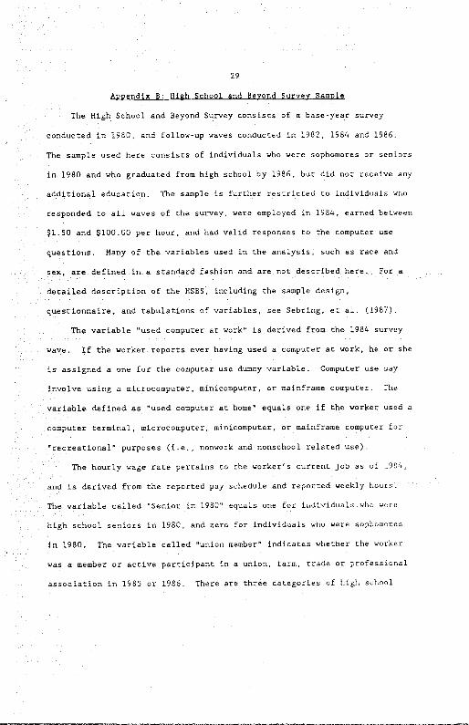
Appendix 5: flush School and Seyond Survey Sample

The High School and Seyond Survey consists of a base-year survey

conducted in 1960, and follow-up waves conducted in 1982, 1984 and 1986,

The sample used here consists of individuals who were sophomores or seniors

in 1980 and who graduated from high school by 1986, but did nor receive any

additional education. The sample is further restricted to individuals who

responded to all waves of the survey. were employed in 1984, earned between

$1.50 and $100.00 per hour, and had valid responses to the computer use

questions, Many of the variables used in the analysis, such as race and

sex, are defined in a standard fashion and are not described here. For a

detailed description of the HSBS, including the sample design,

questionnaire, and tabulations of variables, see Sebring, et al. (1987).

The variable "used computer at work" is derived from the 1984 survey

wave. If the worker reports ever having used a computer at work, he or she

is assigned a one for the computer use dummy variable. Computer use may

involve using a microcomputer, minicomputer, or mainframe computer. The

variable defined as "used computer at home" equals one if the worker used a

computer terminal microcomputer, minicomputer, or mainframe computer for

"recreational" purposes (i.e., nonwork and nonschool related use).

The hourly wags rate pertains to the worker's current job as of l98,

and is derived from the reported pay schedule and reported weekly hours,

The variable called "Senior in 1980" equals one for individuals who w,'re

high school seniors in 1980, and zero for individuals who were sophomores

in 1980. The variable called "union member" indicates whether the worker

was a member or active participant in a union, farm, trade or professional

association in 1985 or 1986. There are three categories of high school

30

types in the survey; general, academic, and vncarinnal. Vocatinnal high

schools are the omitted dummy category. "Utban" measures whether the

worker attended a school in an urban atea.

Patent's education consists of 5 dummy vatah1es for the mnther and

for tho fathet, indicating whether each patent's education is missing, high

school, some college, college, or post college. <Less than high school is

the base group.) In ipso all students were given a 73 minute cognitive

test of vocabulary, readtng, and mathematics. The students' score on the

1982 test is the variable called "achievement test score'. The sophomores

were given a similar test again in 1982. "Grade point average" is the

student's self-reported grade point average in 1982. "Disciplinary

problem" is a dum.'sy variable that indicates whether a student reports

having had a disciplinary problem in high school in rhe last year.

"Disability limits work" is a dummy variable that equals one if a student

reports having a physical disability that limits the kind or amount of work

that ha or abe can do on a job, or that effects his or her chances for more

eduction.

31

Ref erencas

Allen Steven C., "Technology and the Wage Structure " mimeo. North

Carolina State University, May 1991.

Bartel, Ann p. and Frank R. Lichtenberg, "The Comparative Advantage of

Educated Workers in Implementing New Technology " Review of Economics

and Statistics 69 (February 1987); 1-Il,

Berndt, Ernst and Zvi Griliches, "Price Indexes for Microcomputers: An

Exploratory Study," NBER Working Paper No, 3378, June 1990.

Blackburn, McKinley L., David E. Bloom, and Richard B, Freeman, "The

Declinin8 Economic Position of Less Skilled American Men," in Cary

Burtless (ed), A Future of Lousy Jobs? (Washington, DC: Brookings

Institution, 1990).

Blackburn, McKinley L. , David E. Bloom, and Richard B. Freeman, "An Era of

Falling Earnings and Rising Inequality?" The Brookinms Review, Winter

1990-91. pp. 38-03.

Bound, John and George Johnson, "Changes in the Structure of Wages During

the l980s: An Evaluation of Alternative Explanations," NBER Working

Paper No, 2983, May 1989,

Card, David, "The Effects of Unions on the Distribution of Wages:

Redistribution of Relabelling?" Princeton University, Industrial

Relations Section W.P. No. 287, July 1991.

Davis, Steven J. , and John Haltiwanger, "Wage Dispersion Between and Within

U.S. Manufacturing Plants, 1963-1986," NBER Working Paper No,, 3722,

May 1991.

Deaton, Angus, "Panel Data from Time Series of Cross-Sections," Journal of

Econometrics 30, (October/November 1985): 109-126.

32

Criliohes, Zvi, CspitsI-Ski1l Coeplementarity," Review of EconomicThd

Statistics 51 (November 1969): 465-469.

Ileckmsn, James J, and Richard Rohb, Jr., "Alternative Methods for

Evaluating the Impact of Interventions," in J. Heckasn and B. Singer

(eds.), gjtndigl Anal sisLkabQLjfsrket LaCg (Cambridge:

Cambridge University Press, 1985): 156-246.

Hitschhorn, Larry, "Computers and jobs: Servioes and the New Mode of

Production," in Riohard Cyett and David Mowety (eds.), gImDsctof

flcn2kMoa1 Chsn a on Em bent and Rconom4c Growth (Cambridge,

MA: Eallinger Publishing Co., 1988): 377-418.

Juhn, Chinhui, Murphy, Kevin, and Pierce, Erooks, "Wage Inequality and the

Rise in Returns to Skill," manuscript, University of Chfcago,

October 1989.

Katz, Lawrence, and Alan Krueger, "Changes in the Structure of Wages in the

Public and Private Sectors," N8ER Working Paper No. 3667, Match 1991.

Katz, Lawrence, and Kevin Murphy, "Changes in Relative Wages, 1963-1987:

Supply end Demand Factors," mimeo., Mertard University, April 199G.

Katz, Lawrence, and Ana L. Revenge, "Changes in the Structure of Wages: The

United Stares and Japan," Journal of the Japanese and International

Economies 3 (November 1989): S22-5S3.

Kelly Services, Inc., "The Kelly Report on People in the Eleotronic Cffce

III: The Secretary's Role," Troy Michigan, 1984.

Levy, Frank, "Recent Trends in U.S. Earnings and Family Incomes," N8RR

Macroeconomics Annual, vol. 4, edited by Oliv6er Blanchard and Stanley

Fischer, 1989.

33

Lewis, HG., Union Relative Wage Effects: A Spgy (Chicago, IL: University

of Chicago Press, 1986).

Mincer, Jacob, "Human Capital, Technology, and the Wage Structure: What Do

Time Series Show?" NBER Working Paper No, 3581, January 1991,

Murphy, Kevin M. and Finis Welch, 'The Structure of Wages,' manuscript,

University of Chicago, 1988,

Murphy, Kevin M. , and Finis Welch, "Wage Differentials in the l980s: The

Role of International Trade," Economic Incuiry, forthcoming 1991.

Reilly, Kevin T "Human Capital and Information: The Employer Size-Wage

Effect," mimeo. , University of Waterloo, April 1991.

Sebring, Penny, et al. , High School and 8eyond 1980 Sophomore Cohort Third

Follow-Up (1986) Vol. 1, (Washington, DC: Center for Education

Statistics, U.S. Department of Education),

Siegel, Donald, and Zvi Griliches, "Purchased Services, Outsourcing,

Computers, and Productivity in Manufacturing," NBER Working Paper No.

3678, April 1991.